development of low-to mid-rise building structures using

RIGHT:

URL:

CITATION:

AUTHOR(S):

ISSUE DATE:

TITLE:

Development of Low-to Mid-rise BuildingStructures Using Weld-free Built-up ColumnsMade of Ultra-high Strength Steel(Dissertation_全文 )

Lin, Xuchuan

Lin, Xuchuan. Development of Low-to Mid-rise Building Structures Using Weld-free Built-up Columns Made of Ultra-highStrength Steel. 京都大学, 2012, 博士(工学)

2012-09-24

https://doi.org/10.14989/doctor.k17154

許諾条件により要旨・本文は2013-10-01に公開

Development of Low- to Mid-rise Building Structures Using Weld-free Built-up

Columns Made of Ultra-high Strength Steel

September 2012

Xuchuan LIN

- i -

TABLE OF CONTENTS

CHAPTER 1 Introduction

1.1 Background 1-1 1.2 Objective 1-2 1.3 Organization 1-4 REFERENCES 1-6 LIST OF PUBLICATIONS 1-8

CHAPTER 2 Analysis of Prototype Building System Using H-SA700 Steel 2.1 Overview 2-1 2.2 Column Pattern 2-1 2.3 Analyzed Cases and Model 2-2

2.3.1 Parameters of the cases 2-2 2.3.2 Numerical model 2-4

2.4 Modal Analysis 2-6 2.5 Static Nonlinear Pushover Analysis 2-6 2.6 Incremental Dynamic Analysis 2-8

2.6.1 Procedures 2-8 2.6.2 Performance evaluation 2-9

2.7 Summary 2-12 REFERENCES 2-13

CHAPTER 3 Flexural Behavior of Bolted Built-up Columns Using H-SA700 Steel

3.1 General 3-1 3.2 Test Program 3-1

3.2.1 Test specimens 3-1 3.2.2 Test setup 3-4 3.2.3 Instrumentations 3-5 3.2.4 Test procedure 3-6

3.3 Test Results and Analysis 3-6 3.3.1 Behavior 3-7 3.3.2 Elastic stiffness 3-10 3.3.3 Limit states 3-10 3.3.4 Strain distribution 3-11

3.4 Finite Element Analysis 3-13 3.4.1 Model for Specimen H-120 3-13 3.4.2 Yielding initiation and its spreading 3-15 3.4.3 Strain concentration 3-17

3.5 Summary 3-19

- ii -

REFERENCES 3-19 CHAPTER 4 Column Behavior Subjected to Combined Axial Force and Cyclic Lateral Force

4.1 Overview 4-1 4.2 Experimental Program 4-1

4.2.1 Specimens 4-1 4.2.2 Test setup and instrumentations 4-4 4.2.3 Loading protocol 4-5

4.3 Analysis of Test Results 4-5 4.3.1 Failure mode 4-7 4.3.2 Elastic deformation and elastic stiffness 4-8 4.3.3 Strength 4-8

4.4 Finite Element Model and Parameter Study 4-11 4.4.1 Modeling 4-11 4.4.2 Verification 4-13 4.4.3 Parameter study 4-16

4.5 Theoretical Study on Maximum Bending Strength 4-20 4.5.1 Summary on local buckling modes 4-20 4.5.2 Design 4-22 4.5.3 Discussion on the design formula 4-25


CHAPTER 5 Behavior of Unstiffened Local Connections of Column Subjected to Concentrated Forces

5.1 Introduction 5-1 5.1.1 Background and objective 5-1 5.1.2 Organization 5-3

5.2 Local tension test 5-3 5.2.1 Specimen and design 5-3 5.2.2 Test setup 5-5 5.2.3 Test results and analysis 5-6 5.2.4 Finite element analysis 5-7

5.3 Local compression test 5-11 5.3.1 Specimens 5-11 5.3.1 Test setup and instrumentations 5-11 5.3.3 Test results and analysis 5-13 5.3.4 Finite element analysis 5-14


- iii -

CHAPTER 6 Behavior of Bolted Beam-to-column Connections 6.1 Introduction 6-1

6.1.1 Objectives 6-1 6.1.2 Organization 6-1

6.2 Connection Patterns 6-2 6.3 Test Program 6-3

6.3.1 Specimen 6-3 6.3.2 Test setup and loading protocol 6-5 6.3.3 Instrumentation 6-5

6.4 Test Results and Analysis 6-6 6.4.1 Global behavior 6-7 6.4.2 Column 6-8 6.4.3 Beam 6-9 6.4.4 Panel zone 6-9 6.4.5 CFEP zone and energy dissipation 6-12

6.5 Finite element analysis 6-13 6.5.1 Modeling 6-13 6.5.2 Verification 6-14 6.5.3 Analysis 6-15


CHAPTER 7 Design for Local Connection of Bolted Built-up Columns Under Concentrated Tensile Force

7.1 Overview 7-1 7.2 Theoretical Study 7-1

7.2.1 Assumptions and procedures 7-1 7.2.2 Unstiffened Connection 7-2 7.2.2 Stiffened Connection 7-5

7.3 Verification and Discussions 7-7 7.3.1 Local tension test 7-7 7.3.2 Beam-to-column connections 7-8

7.4 Summary 7-10 REFERENCES 7-10 Appendix A. Formulae for Local Tension of Unstiffened Connection 7-11 Appendix B. Formulae for Local Tension of Stiffened Connection 7-13

CHAPTER 8 Summary and Conclusions 8-1

8.1 Summary and Conclusions 8-1 8.2 Future Work 8-5

ACKNOWLEDGEMENT

- iv -

1 - 1

CHAPTER 1

Introduction

1.1 Background H-SA700 steel The most common steel grades used for building construction, such as JIS SS400, SN400, SN490 in Japan, and ASTM A36 and A529 in the U.S., have a specified minimum tensile strength of 400 to 500 MPa. Steel with substantially higher strength has been available but has been limited to special applications. For example, steel with a minimum tensile strength of 800 MPa and good weldability has been used extensively in long-span bridges [1]. A large number of jumbo pipes with a tensile strength of 780 MPa and wall thickness of 100 mm are used in the Tokyo Sky Tree tower, which stands as the tallest free-standing tower in the world at 634 meters high [2]. For such special applications, the higher strength is achieved either by increasing the amount of alloying elements in the steel, or by performing heat treatment.

H-SA700 steel is a high-strength structural steel that is manufactured by a thermo-mechanical control process (TMCP) technology [3]. Because H-SA700 steel achieves very high strength without significantly altering its chemical composition (i.e., without increasing alloying elements) and without introducing intensive heat treatment, this steel is more environmentally friendly (because of lower discharge of CO2) and more suitable for mass production and recycling (because of low alloying elements) than conventional high-strength steel. As an illustration, Table 1.1 shows the chemical compositions of high-strength steels made by conventional method and new method (TMCP) in laboratory [4], respectively. The demand for the alloying elements is significantly reduced in the method to make H-SA700 steel.

H-SA700 steel has a specified yield strength range of 700 to 900 MPa and a specified tensile strength range of 780 to 1,000 MPa [4]. For illustration, Figure 1.1 shows stress-strain curves for H-SA700 and SS400 steel established from tension coupon tests. SS400 steel is a commonly used mild carbon steel in Japan, and is equivalent to A36 steel used in the US. Compared to the conventional SS400, H-SA700 offers three times the yield strength, although the increase in yield-to-tensile strength ratio and reduction in the rupture elongation indicate that ductility is compromised.

1 - 2

Table 1.1 Chemical compositions of high-strength steels made by different methods in laboratory Method C Si Mn P S Cu Ni Cr Mo V

Conventional 0.108 0.25 0.94 0.012 0.004 0.2 0.79 0.49 0.39 0.04 TMCP 0.183 0.4 1.44 0.024 0.008 0.02 0.02 0.49 <0.01 <0.01

Research on steel constructions using H-SA700 steel

The H-SA700 steel was developed as part of a large multi-industry effort to realize structural systems that enable continuous use even after very rare earthquakes. Takanashi et al. achieved this goal by designing a dual frame system composed of a stiff external shell and a soft internal frame which are connected by hydraulic dampers [5]. The concept was implemented in a full-scale building that underwent extensive vibration testing. In this building, the high strength of H-SA700 was exploited to form the stiff external truss shell, while the large elastic deformation limit of H-SA700 was exploited to design the soft internal frame. Along the same lines, a few other studies were conducted for the promotion of H-SA700. Shinsai et al. [6] developed a cruciform built-up column of H-SA700 using under-matching fillet welds. Fujimaki et al. [7] examined welded beam-to-column connections of H-SA700 in which horizontal haunches were added to reduce the strains at the welded sections. Qiao et al. [8], Sato et al. [9], and Tanaka & Sakai [10] investigated the possibilities of columns, beams, and beam-to-column connections made of H-SA700 using high-strength bolts.

0

300

600

900

0.00 0.10 0.20 0.30

Stre

ss (M

Pa)

Strain

H-SA700

SS400

Figure 1.1 Stress-strain relationship.

1.2 Objective The research target is to develop a new structural steel system that extends the benefits offered by the H-SA700 steel. A system is sought that (1) minimizes energy consumption during manufacturing, fabrication, and construction, (2) maximizes reusability and recyclability, (3) enables continuous use after major earthquakes, and (4) most notably, and unlike previous development efforts focused on H-SA700 [5~10], targets low- to mid-rise buildings (not special

1 - 3

structures) in which the majority of structural steel is consumed. According to a survey of steel buildings in Japan, nearly 95% of the floor area constructed between years 1986 and 2009 belonged to buildings of 10 stories or fewer [11], as shown in Figure 1.2.

Floo

r are

a co

nstru

cted

0%

10%

20%

30%

40%

50%

60%

70%

80%

90%

100%

86 87 88 89 90 91 92 93 94 95 96 97 98 99 00 01 02 03 04 05 06 07 08 09

Single Story

2 Stories

3 to 5 Stories

16+10 to 15

6 to 9

Fiscal Year Figure 1.2 Breakdown of floor area for steel structures [11].

In order to achieve these goals, a new structural system using H-SA700 steel was proposed, and

the conceptual sketch of the envisioned steel system is shown in Figure 1.3. The system is achieved by connecting columns, beams, and dampers using only bolts and no welds, so that all the components can be replaced, reused, and recycled. The beams can be either conventional beams using mild steel or new beams using high-strength steel. In this study, the beams are assumed to be the conventional beams using mild steel. The columns are built up from H-SA700 steel plates, either flat or cold bent, using bolts exclusively and no welds. The columns are provided with sufficiently large strength to keep them elastic under very rare earthquake events. In appearance, these columns resemble older built-up sections from the early 20th century [12] except that rivets are replaced by high-strength bolts. In this system, dampers are intended to dissipate most of the energy, and beams may also dissipate more energy under a rare earthquake event, but the column should keep elastic.

The dissertation aims at future research toward the practical use of the new structural system. The basic research issues explored in the dissertation are as follows:

(1) How to design the structure to make better use of the ultra-high strength steel, and how to ensure the continuous use of the structure even after very rare earthquakes;

(2) How to design and fabricate the bolted built-up columns; (3) How to design connections to the new columns, such as the beam-to-column connections

and local connections. Accordingly, three research objectives are chosen in this study. The first is to identify the roles

of different types of members in the prototype structure, and evaluate the seismic performance of the structural system. The second is to seek and propose feasible bolted built-up column patterns,

1 - 4

investigate the behavior of the proposed column, and develop the design method for the column. The third is to design appropriate bolted connections (specifically beam-to-column connections) including its bolted stiffeners, examine the connection behavior, and investigate the corresponding design.

Damper

Conventional Beam using mild steel

New column using high-strength steel

Moment or shear connection

Figure 1.3 Concept of structural system.

1.3 Organization

Bolted Built-up Columns

Flexural Behavior(Chapter 3)

Combined Bending and Compression

(Chapter 4)

Local Compression/Tension

(Chapter 5)

Beam-to-Column Connection(Chapter 6)

Connection Design(Chapter 7)

Structural SystemUsing H-SA700 Steel

(Chapter 2)

Column Design(Chapter 4)

Bolted Connections

Figure 1.4 Relationship between different chapters.

1 - 5

This dissertation consists of eight chapters. Chapter 1 presents the background of this study, and Chapter 8 is the summary and conclusions. As shown in Figure 1.4, Chapters 2 to 7 constitute the main body of the dissertation: (1) the column pattern and prototype building; (2) flexural behavior of the bolted built-up columns; (3) column behavior subjected to combined axial force and cyclic lateral force, and column design method; (4) behavior of unstiffened built-up column subjected to concentrated force; (5) behavior of bolted beam-to-column connections; and (6) design for local connection of the column under concentrated tensile force. The contents of the six chapters are summarized below.

In Chapter 2, Eight different bolted built-up column patterns, including both closed and open sections, are designed using “pate only, bolt only” strategy, and one of them is selected for its good balance between the mechanical performance and fabrication feasibility. Three braced frame structures are designed to examine the performance of the proposed structural system. One is a conventional braced frame, and the other two are the candidate prototype braced frames using ultra-high strength steel for the columns. One candidate prototype frame used flexible columns of small section, while the other used strong columns of doubled strength. A series of numerical analyses, including modal analysis, static nonlinear pushover analysis and incremental dynamic analysis, are conducted. Different aspects of the structural performance, such as the yield story drift, maximum story drift, and maximum residual deformation, are evaluated. One of the candidate structures is chosen as the prototype of the research.

Chapter 3 summarizes study on the flexural behavior of the built-up columns, whose objective is to establish the flexural properties and design method of the columns. Three column specimens are fabricated and subjected to cyclic lateral loading. The test results, such as the section stiffness, yield bending moment, plastic bending moment, rupture, local buckling of the flanges, bolt slippage, are used to identify the key limit states and to develop a design methodology that addresses the unique behavior of the built-up columns. Local detailed strain distribution is investigated by the strain gauge data, and the detailed issues, such as local strain concentration and plane-section assumption, are investigated. Finite element simulation is used to explore the experimental findings, and the issues about the yield mechanism over a group of reduced sections and the local strain concentration at the vicinity of bolt holes are investigated.

Chapter 4 presents a study on the column behavior subjected to combined axial force and cyclic lateral force. First, a laboratory test on the column behavior is described and analyzed. Five specimens are designed for three parameters, e.g., the directions of the lateral loads, bolt pitch to fabricate the column and magnitude of the axial force exerted on the column. The specimens are reduced in dimension from the prototype section tested in Chapter 3. Effects of various parameters on column behavior, such as the stiffness, elastic deformation capacity, strength and failure modes, are evaluated. Second, a finite element model is proposed, and verified with the five specimens. A parameter study on the strength, damage details of the specimens and the effect of boundary conditions at the bottom of the column is carried out. Third, failure modes are summarized, and theoretical formulae for the estimation of the column strength are proposed.

In Chapter 5, two series of unstiffened connection behavior are investigated, one for local

1 - 6

connections under a perpendicular tensile force (local tension test), and the other under a compressive force (local compression test). Both of laboratory tests and finite element simulations are carried out to examine the strength, deformation mode, and yield zone of the column. The ways of reinforcing the column with stiffeners are sought and proposed based on the analysis of the column behavior.

In Chapter 6, both an experimental study and finite element analysis are conducted to study the behavior of the beam-to-column connections. First, two types of bolted stiffeners are proposed: one is fabricated with three Tees connecting each other (Tee stiffeners), and the other with two angles overlapping each other (Angle stiffeners). Second, tests of four large-scale beam-to-column connection specimens are carried out. The test setup, loading protocol of cyclic loading, and instrumentations (strain gauges and displacement transducers), are introduced. Third, test results and their analyses are presented. Local behavior, such as local distortion in the column flange and local buckling in the beam, are compared between the connections. The strength, deformation, and energy dissipation of the connecting components are also evaluated. The effect of stiffeners on the reinforcement of the connection is investigated. Finally, a finite element model, which adopts contact between all connecting components, is proposed, and the plasticity and energy dissipation in various parts of the specimen are quantified.

In Chapter 7, the design formulas for local connections of columns under concentrated tensile force are established. The theoretical studies based on the upper bound theorems of plastic analysis are conducted to achieve the design formulas for the strength of the bolted built-up column under perpendicular tensile force. Two possible yield patterns (collapse mechanisms) are considered for unstiffened connections, and the minimum strength for each pattern is obtained. Three possible spatial yield patterns (collapse mechanisms) for stiffened connections are investigated, and the conditions for the application of each pattern are discussed.

REFERENCES [1] Miki C (2002). High strength and high performance steels and their use in bridge structures.

Journal of Constructional Steel Research, 58:3-20. [2] Japan Iron and Steel Federation and Japanese Society of Steel Construction (2010). Tokyo Sky

Tree-high-strength steel pipe for antenna tower. Steel Construction Today&Tomorrow, 31:14-15.

[3] Nishioka, K (2000). Market requirements of thermo-mechanically processed steel for the 21st century. Steel World, 5(1):61-67.

[4] Yoshida Y, Obinata T, Nishio M, Shiwaku T (2009). Development of high-strength (780N/mm2) steel for building systems. International Journal of Steel Structures, 9(4): 285-289.

[5] Takanashi K, Miyazaki K, Yamazaki K, Shimura Y (2010). A new structural system using innovative high-strength steel aiming at zero earthquake damage. Structural Engineering International, 20(1): 66-71.

1 - 7

[6] Shinsai N, Sato A, Suita K (2010). Experiments for performance evaluation of high strength steel built-up members made by under matched welds: Part 2 Cruciform frame tests. Summaries of Technical Papers of AIJ Annual Meeting, 2010;C-1:675-676. (in Japanese).

[7] Fujimaki Y, Nakagomi T, Kawabata Y, Sakino Y (2011). Study on strength and deformation capacity of beam-to-column welded connection using H-SA700 for beam and column: Part 1 Outline of experiment. Preprints of the National Meeting of JWS 2011;89:220-221. (in Japanese).

[8] Qiao Q, Kawano A, Tsuda K, Kido M (2009). Experimental study on the compression strength of column: Design of weld-free built-up structural members using 780N/mm^2 high strength steels (H-SA700)-Part1. Summaries of Technical Papers of AIJ Annual Meeting. C-1, 2009: 597-598. (in Japanese)

[9] Sato A, Kimura K, Suita K (2009). Development of weld-free beam-to-column connection of H-SA700A high strength steel for building structures. Journal of Structural and Construction Engineering, 74(646): 2355-2363. (in Japanese).

[10] Tanaka T, Sakai J (2010). Bending test of composite beam using H-SA700A high strength steel. Summaries of technical papers of AIJ Annual Meeting 2010; C-1:1383-1384. (in Japanese)

[11] Japan Iron and Steel Federation. Statistics and figures on steel buildings. http://www.jisf.or.jp/business/tech/build/index.html

[12] Wermiel SE (2009). Introduction of steel columns in US buildings, 1862-1920. Engineering History and Heritage, 162 Issue EHI: 19-27.

1 - 8

LIST OF PUBLICATIONS

1. PhD Research

Journal paper:

[1] Lin X, Chung YL, Okazaki T, Nakashima M. Experimental study on flexural capacity of built-up

columns using high-strength steel. JSSC Journal of Constructional Steel, 2011, No.19,

pp685-690.

[2] Lin X, Okazaki T, Chung YL, Nakashima M. Flexural performance of bolted built-up columns

constructed of H-SA700 steel. Journal of Constructional Steel Research. (under review)

[3] Lin X, Hayashi K, Okazaki T, Enomoto R, Nakashima M. Experimental study on built-up

columns using high-strength steel subjected to combined bending and axial force. JSSC Journal

of Constructional Steel, 2012, No.20. (under review)

[4] Hayashi K, Okazaki, T, Lin X, Nakashima M. Bending Performance of bolted built-up columns

made of H-SA700 steel. Steel Construction Engineering. (under review, in Japanese)

International conference paper:

[1] Lin X, Chung YL, Okazaki T, Nakashima M. Weld-free columns using ultra-high-strength

steel: Experimental study on flexural performance. 6th European Conference on Steel and

Composite Structures, August 31-September 2, 2011, Budapest, Hungary.

[2] Lin X, Chung YL, Okazaki Y, Nakashima M. Beam-to-column connection for built-up column

using ultra-high-strength steel. Behavior of Steel Structures in Seismic Areas 2012, Santiago,

Chile, January 9 - 11, 2012.

[3] Lin X, Okazaki T, Hayashi K, Chung YL, Nakashima M. Combined compression and bending

behavior of built-up columns using high-strength steel, Proc. the 15th World Conference on

Earthquake Engineering, September 24-28, 2012, Lisbon, Portugal. (accepted)

Domestic conference paper:

[1] Lin X, Okazaki T, Chung YL, Nagae T, Matsumiya T, Nakashima M. Retrofit evaluation on

local fracture failure of welded moment-resisting connection. Summaries of Technical Papers of

1 - 9

Annual Meeting, Architectural institute of Japan, Sep. 2010, C-1:793-794.

[2] Lin X, Chung YL, Okazaki T, Nakashima M. Flexural performance of built-up weld-free

columns using ultra-high-strength steel: Part I: Design and test. Summaries of Technical Papers

of Annual Meeting Kinki branch, AIJ, No.51, pp.169-172, June, 2011.

[3] Chung YL, Lin X, Okazaki T, Nakashima M. Flexural performance of built-up weld-free

columns using ultra-high-strength steel: Part II: Test Results. Summaries of Technical Papers

of Annual Meeting Kinki branch, AIJ, No.51, pp.173-176, June, 2011.

[4] Lin X, Chung YL, Okazaki T, Nakashima M. Test on flexural capacity of built-up weld-free

columns using ultra-high-strength steel: Part I: Design and test. Summaries of Technical Papers

of Annual Meeting, AIJ, Aug. 2011, C-1:675-676.

[5] Chung YL, Lin X, Okazaki T, Nakashima M. Test on flexural capacity of built-up weld-free

columns using ultra-high-strength steel: Part II: Test Results. Summaries of Technical Papers of

Annual Meeting, AIJ, Aug. 2011, C-1:677-678.

[6] Hayashi K, Lin X, Chung YL, Okazaki T, Enomoto R, Nakashima M. Beam-to-column

connections for bolted built-up columns made of H-SA700 steel: Part 1 Test results and analysis.

Summaries of Technical Papers of Annual Meeting Kinki branch, AIJ, No.52,425-428, June,

2012.

[7] Lin X, Okazaki T, Chung YL, Hayashi K, Enomoto R, Nakashima M. Beam-to-column

connections for bolted built-up columns made of H-SA700 steel: Part 2 Test plan. Summaries of

Technical Papers of Annual Meeting Kinki branch, AIJ, No.52, 429-432, June, 2012.

2. Undergraduate and Master Research

Journal paper:

[1] Lin X, Feng P, Ye L. Design methodology for the space truss of CFRP strengthened aluminum

members. Industrial Construction, 2007, Suppl.:120-125.

[2] Pan P, Lin X, Wang Z, Wang W, Ye L, Qian J. Experimental study on ring-beam connections

of steel reinforced concrete columns and reinforced concrete beams. Journal of Building

Structures, 2008,(S1):226-230. (in Chinese)

[3] Lu X, Lin X, Ye L. Finite element modeling and its application in structural analysis. Journal

of Huazhong University of Science and Technology (Urban Science Edition), 2008, 25(4): 76-80.

(in Chinese)

1 - 10

[4] Feng P, Lin X, Qian P, Ye L. Mechanical behavior and design methodology of CFRP

strengthened aluminium Members. Progress in Steel Building Structures, 2008, 10(1):34-43. (in

Chinese)

[5] Ye L, Qu Z, Ma Q, Lin X, Lu X, Pan P. Study on ensuring the strong column-weak beam

mechanism for RC frames based on the damage analysis in the Wenchuan Earthquake. Building

Structure, 2008, 38(11): 52-59. (in Chinese)

[6] Lin X, Pan P, Ye L, Lu X, Zhao S. Analysis of the damage mechanism of a typical RC frame in

Wenchuan Earthquake. China Civil Engineering Journal, 2009,(05):13-20. (in Chinese)

[7] Lin X, Lu X, Miao Z, Ye L, Yu Y, Shen L. Finite element analysis and engineering application

of RC core-tube structures based on the multi-layer shell elements. China Civil Engineering

Journal, 2009,(03):49-54. (in Chinese)

[8] Wang Z, Lin X, Wang W, Pan P, Ye L, Qian J. Static tests on ring-beam connections for SRC

columns and RC beams under symmetrical load. Building Structure, 2009,(08):36-39,43. (in

Chinese)

[9] Ye L, Feng P, Lin X, Qi Y. Analysis of safety margin indices for structural members with FRP.

China Civil Engineering Journal, 2009,(09):21-31. (in Chinese)

[10] Lin X, Lu X, Ye L. Multi-scale finite element modeling and its application in the analysis of a

steel-concrete hybrid frame. Chinese Journal of Computational Mechanics, 2010,

(03):469-475,495. (in Chinese)

[11] Lu X, Lin X, Ye L, Yi Li, Tang D. Numerical models for earthquake induced progressive

collapse of high-rise buildings. Engineering Mechanics, 2010,(11):64-70. (in Chinese)

[12] Ye L, Lin X, Qu Z, Lu X, Pan P. Evaluating Method of Element Importance of Structural

System Based on Generalized Structural Stiffness. Journal of Architecture and Civil

Engineering, 2010,(01):1-6,20. (in Chinese)

[13] Feng P, Chu M, Lin X, Hou J, Liu Y. Calculation and test for strengths of cold-formed

thin-wall steel reinforced concrete slabs. Journal of Tsinghua University (Science and

Technology), 2010,(09):1325-1329. (in Chinese)

[14] Lin X, Ye L. Study on optimization of seismic design for RC frames based on member

importance index. Journal of Building Structures, 2012, 33(06):16-21. (in Chinese)

[15] Pan P, Lin X, Lam A, Chen H, Ye L. Monotonic loading tests of ring-beam connections for steel

1 - 11

reinforced concrete columns and reinforced concrete beams. Journal of Structural Engineering,

ASCE. (under review)

International conference paper:

[1] Lu X, Lin X, Ma Y, Li Y, Ye L. Numerical simulation for the progressive collapse of concrete

building due to earthquake, Proc. the 14th World Conference on Earthquake Engineering,

October 12-17, 2008, Beijing, China, CDROM.

[2] Lu X, Lin X, Ye L. Simulation of structural collapse with coupled finite element-discrete

element method, Proc. Computational Structural Engineering, Jun. 22-24, 2009, Springer,

Shanghai:127-135.

Domestic conference paper:

[1] Ye L, Lin X, Feng P. Economic analysis of the safety degree of reinforced-concrete beams.

Proceeding of 1st National Conference on Building Structure Technology, June, 2006, Beijing.

(in Chinese)

Book Chapters:

[1] Lu X, Lin X. Chapters 4 and 6 of Elasto-Plastic Analysis of Buildings Against Earthquake,

(Edited by Lu X, Ye L, Miao Z, et al. China Architecture and Building Press, Beijing, 2009.) (in

Chinese)

1 - 12

2 - 1

CHAPTER 2

Analysis of Prototype Building System Using H-SA700 Steel

2.1 Overview A new building system using ultra-high-strength steel was proposed for low- to mid- rise buildings. The objective for this chapter is to figure out preliminary details of the structural system, and give insight to its structural performance. The contents of this chapter are as follows:

(1) A bolted built-up column pattern, using “plate only, bolt only” strategy, was developed from eight different bolted column patterns, including both closed and open sections.

(2) Three structures were designed to examine the performance of the proposed structural system. One is a conventional braced frame, and the other two are the candidate prototype structures using ultra-strength-steel for the columns.

(3) A numerical model was introduced, and a series of numerical analyses, including modal analysis, static nonlinear pushover analysis, and incremental dynamic analysis, were conducted. Various aspects of the structural performance were evaluated, and one of the candidate structures was chosen for the research to follow.

2.2 Column Pattern Figure 2.1 presents examples of the weld-free column patterns examined, which ranged from closed sections (A to B) to opened sections (E to H). Closed sections offer excellent torsional stiffness and biaxial bending properties, but obstruct bolted construction. Open sections provide poor torsional properties and poor local buckling strength, but offer easy access for bolted construction. The semi-closed sections C and D combine the superior cross-sectional properties of closed sections with the superior constructability of opened sections. Section C may be viewed as a heavier variety of Section D. Therefore, Section D was chosen as the focus of this research. Section D combines two flat plates, acting as the flanges, and two channels, acting as a dual web, connected by high-strength bolts. The bolts are evenly pitched and fully tightened prior to erection, except where

2 - 2

connections occur. At the connections to the beams or to the foundation, the bolt-hole locations are adjusted to the connection. These bolts are delivered loose to the construction site and serve as the fasteners to assemble the columns and fasten the connections.

A B C D E F G H

Figure 2.1 Built-up column patterns.

The “Plate only, Bolt only” strategy was applied to fabricate the adopted column pattern. The column comprises two flange plates (called exterior plates hereafter) and two interior channels. The channels are also cold formed from the same plates. The section components are connected by bolts, as shown in Figure 2.2.

Cold-formed channels as dual web

Flat plates as flanges

Built-up usinghigh-strength bolts

Figure 2.2 Fabrication of the proposed built-up section.

2.3 Analyzed Cases and Model

2.3.1 Parameters of the cases

Three planar braced frames, Frame C-B, Frame H-B and Frame SH-B, were designed for examining the benefits and feasibility of using high-strength steel. All of the frames share the same elevation

2 - 3

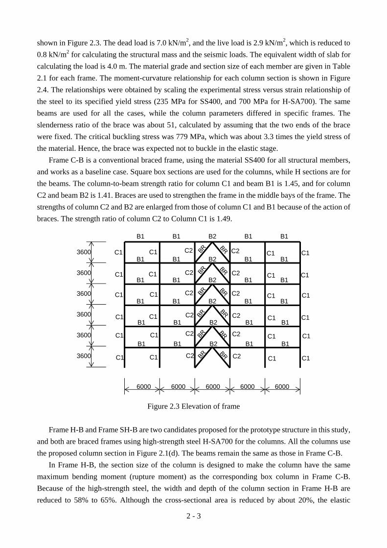
shown in Figure 2.3. The dead load is 7.0 kN/m2, and the live load is 2.9 kN/m2, which is reduced to 0.8 kN/m2 for calculating the structural mass and the seismic loads. The equivalent width of slab for calculating the load is 4.0 m. The material grade and section size of each member are given in Table 2.1 for each frame. The moment-curvature relationship for each column section is shown in Figure 2.4. The relationships were obtained by scaling the experimental stress versus strain relationship of the steel to its specified yield stress (235 MPa for SS400, and 700 MPa for H-SA700). The same beams are used for all the cases, while the column parameters differed in specific frames. The slenderness ratio of the brace was about 51, calculated by assuming that the two ends of the brace were fixed. The critical buckling stress was 779 MPa, which was about 3.3 times the yield stress of the material. Hence, the brace was expected not to buckle in the elastic stage.

Frame C-B is a conventional braced frame, using the material SS400 for all structural members, and works as a baseline case. Square box sections are used for the columns, while H sections are for the beams. The column-to-beam strength ratio for column C1 and beam B1 is 1.45, and for column C2 and beam B2 is 1.41. Braces are used to strengthen the frame in the middle bays of the frame. The strengths of column C2 and B2 are enlarged from those of column C1 and B1 because of the action of braces. The strength ratio of column C2 to Column C1 is 1.49.

B1 B1 B1 B1B2

B1 B1 B1 B1B2

B1 B1 B1 B1B2

B1 B1 B1 B1B2

B1 B1 B1 B1B2

B1 B1 B1 B1B2

C1 C1

C1 C1

C1 C1

C1 C1

C1 C1

C1 C1

C1 C1

C1 C1

C1 C1

C1 C1

C1 C1

C1 C1

C2

C2

C2

C2

C2

C2

C2

C2

C2

C2

C2

C2

6000

3600

3600

3600

3600

3600

3600

6000 6000 6000 6000

Figure 2.3 Elevation of frame Frame H-B and Frame SH-B are two candidates proposed for the prototype structure in this study,

and both are braced frames using high-strength steel H-SA700 for the columns. All the columns use the proposed column section in Figure 2.1(d). The beams remain the same as those in Frame C-B.

In Frame H-B, the section size of the column is designed to make the column have the same maximum bending moment (rupture moment) as the corresponding box column in Frame C-B. Because of the high-strength steel, the width and depth of the column section in Frame H-B are reduced to 58% to 65%. Although the cross-sectional area is reduced by about 20%, the elastic

2 - 4

deformation capacity of the column is significantly enlarged to about five times because of a combination of smaller sections and higher strength steel.

In Frame SH-B, the section size of the column is determined by making the column have the same section area as the corresponding box column in Frame C-B. With the same section area, the columns in SH-B have a larger strength (about two times) and elastic deformation capacity (about four times). Meanwhile, the bending stiffness of the columns using high-strength steel is smaller, which may make the structure more flexible.

Table 2.1 Materials and sections (unit: mm).

Parameter Frame C-B (Conventional columns)

Frame H-B (Flexible columns)

Frame SH-B (Strong columns)

Column C1

Material SS400 H-SA700 H-SA700 Section □-400x400x12 -230x230x12 -300x300x12

Column C2

Material SS400 H-SA700 H-SA700 Section □-400x400x19 -260x260x16 -300x300x16

Beam B1

Material SS400 SS400 SS400 Section H-400x200x9x22 H-400x200x9x22 H-400x200x9x22

Beam B2

Material SS400 SS400 SS400 Section H-450x200x12x25 H-450x200x12x25 H-450x200x12x25

BR Material SS400 SS400 SS400 Section □-150x150x12 □-150x150x12 □-150x150x12

0

500

1000

1500

2000

2500

3000

0 0.2 0.4 0.6 0.8 1Curvature (rad/m)

Mom

ent (

kN.m

)

C2 (SH-B)

C1 (SH-B)

C1 (C-B)

C1 (H-B)

C2 (C-B)

C2 (H-B)

Figure 2.4 Strength of column sections.

2.3.2 Numerical model

The numerical analyses, including modal analysis, static pushover analysis, and dynamic analysis, were conducted in the finite element software MSC.Marc 2008 [1]. The model used for the analysis

2 - 5

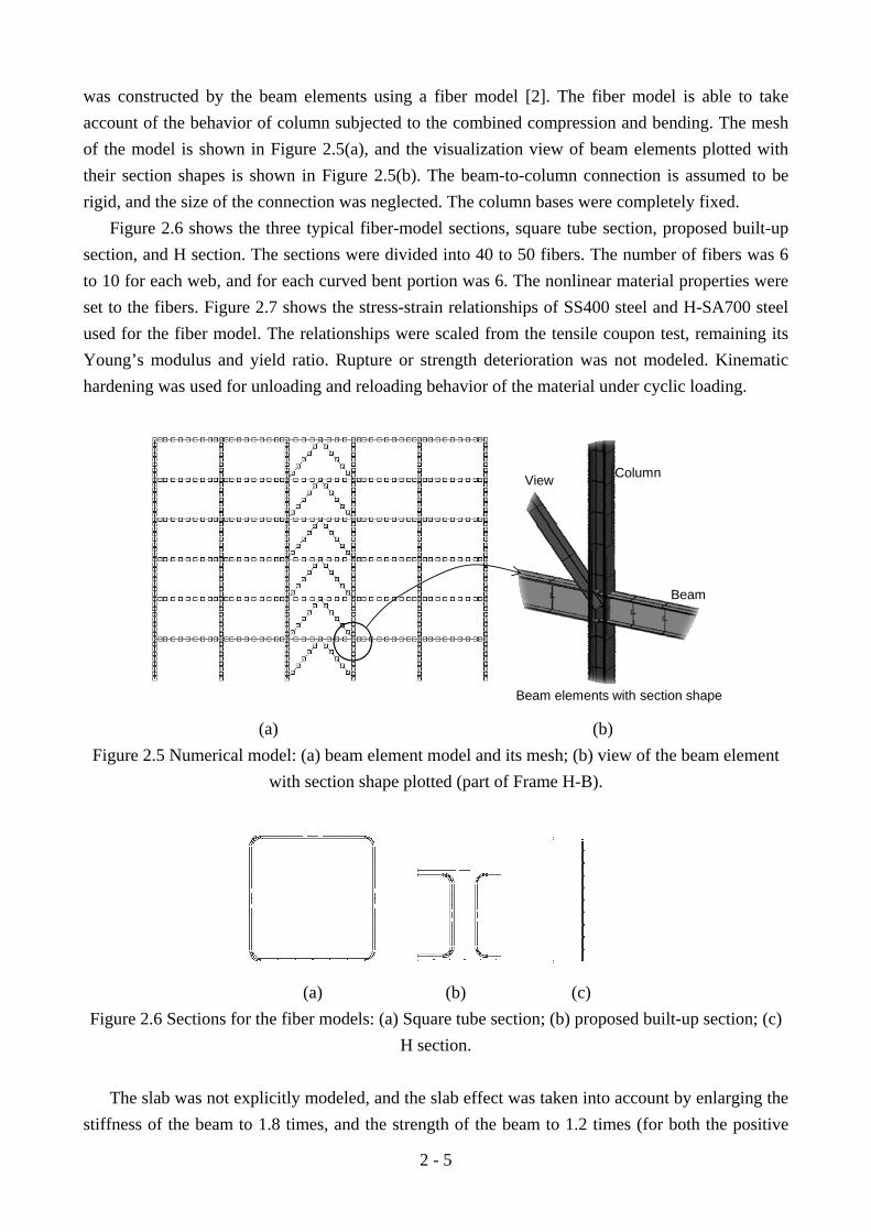
was constructed by the beam elements using a fiber model [2]. The fiber model is able to take account of the behavior of column subjected to the combined compression and bending. The mesh of the model is shown in Figure 2.5(a), and the visualization view of beam elements plotted with their section shapes is shown in Figure 2.5(b). The beam-to-column connection is assumed to be rigid, and the size of the connection was neglected. The column bases were completely fixed.

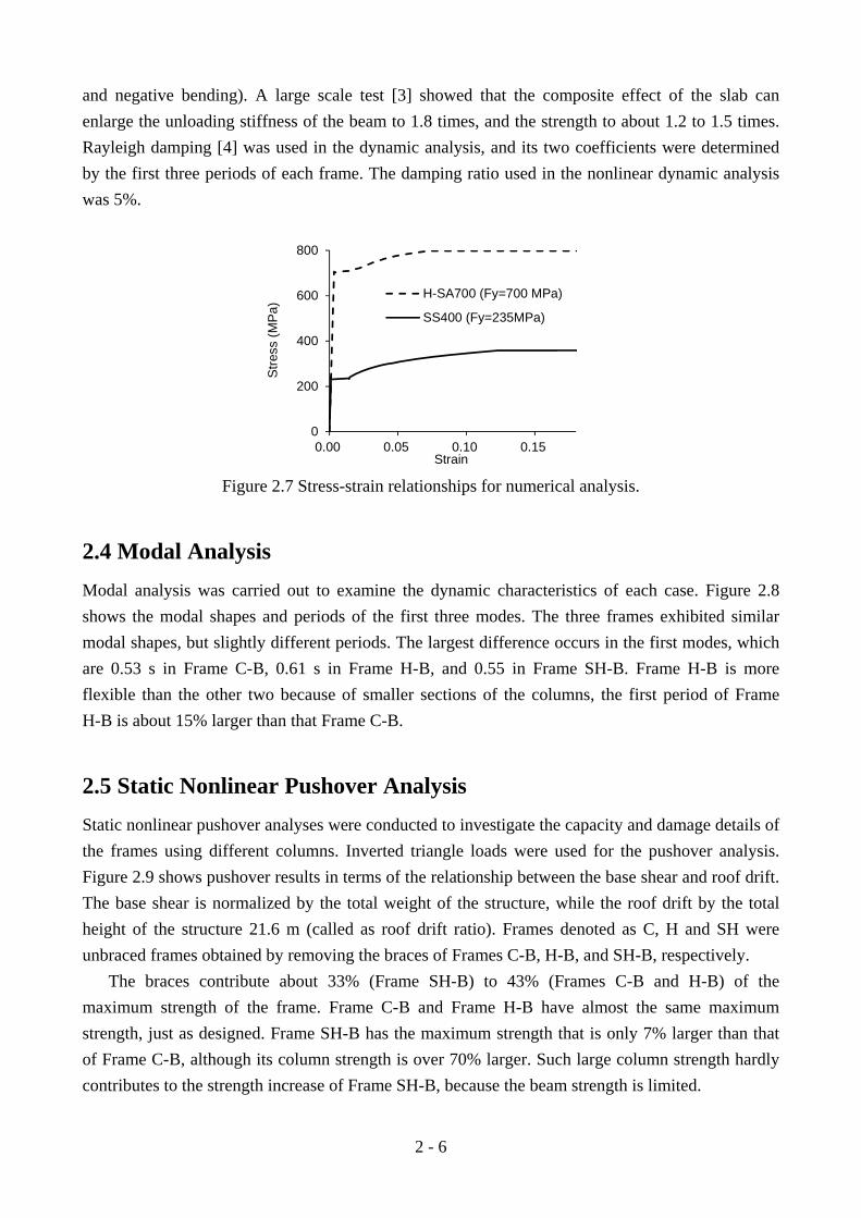
Figure 2.6 shows the three typical fiber-model sections, square tube section, proposed built-up section, and H section. The sections were divided into 40 to 50 fibers. The number of fibers was 6 to 10 for each web, and for each curved bent portion was 6. The nonlinear material properties were set to the fibers. Figure 2.7 shows the stress-strain relationships of SS400 steel and H-SA700 steel used for the fiber model. The relationships were scaled from the tensile coupon test, remaining its Young’s modulus and yield ratio. Rupture or strength deterioration was not modeled. Kinematic hardening was used for unloading and reloading behavior of the material under cyclic loading.

Beam elements with section shape

Beam

ColumnView

(a) (b)

Figure 2.5 Numerical model: (a) beam element model and its mesh; (b) view of the beam element with section shape plotted (part of Frame H-B).

(a) (b) (c)

Figure 2.6 Sections for the fiber models: (a) Square tube section; (b) proposed built-up section; (c) H section.

The slab was not explicitly modeled, and the slab effect was taken into account by enlarging the

stiffness of the beam to 1.8 times, and the strength of the beam to 1.2 times (for both the positive

2 - 6

and negative bending). A large scale test [3] showed that the composite effect of the slab can enlarge the unloading stiffness of the beam to 1.8 times, and the strength to about 1.2 to 1.5 times. Rayleigh damping [4] was used in the dynamic analysis, and its two coefficients were determined by the first three periods of each frame. The damping ratio used in the nonlinear dynamic analysis was 5%.

0

200

400

600

800

0.00 0.05 0.10 0.15

Stre

ss (M

Pa)

Strain

H-SA700 (Fy=700 MPa)

SS400 (Fy=235MPa)

Figure 2.7 Stress-strain relationships for numerical analysis.

2.4 Modal Analysis Modal analysis was carried out to examine the dynamic characteristics of each case. Figure 2.8 shows the modal shapes and periods of the first three modes. The three frames exhibited similar modal shapes, but slightly different periods. The largest difference occurs in the first modes, which are 0.53 s in Frame C-B, 0.61 s in Frame H-B, and 0.55 in Frame SH-B. Frame H-B is more flexible than the other two because of smaller sections of the columns, the first period of Frame H-B is about 15% larger than that Frame C-B.

2.5 Static Nonlinear Pushover Analysis Static nonlinear pushover analyses were conducted to investigate the capacity and damage details of the frames using different columns. Inverted triangle loads were used for the pushover analysis. Figure 2.9 shows pushover results in terms of the relationship between the base shear and roof drift. The base shear is normalized by the total weight of the structure, while the roof drift by the total height of the structure 21.6 m (called as roof drift ratio). Frames denoted as C, H and SH were unbraced frames obtained by removing the braces of Frames C-B, H-B, and SH-B, respectively.

The braces contribute about 33% (Frame SH-B) to 43% (Frames C-B and H-B) of the maximum strength of the frame. Frame C-B and Frame H-B have almost the same maximum strength, just as designed. Frame SH-B has the maximum strength that is only 7% larger than that of Frame C-B, although its column strength is over 70% larger. Such large column strength hardly contributes to the strength increase of Frame SH-B, because the beam strength is limited.

2 - 7

T1=0.53s T2=0.18s T3=0.099s (a)

T1=0.61s T2=0.20s T3=0.110s

(b)

T1=0.55s T2=0.18s T3=0.104s

(c) Figure 2.8 First three modes from modal analysis: (a) Frame C-B; (b) Frame H-B; (c) Frame SH-B.

Base

she

ar /

Tota

l wei

ght

Roof drift ratio (rad)

0

0.1

0.2

0.3

0.4

0.5

0.6

0 0.01 0.02 0.03 0.04 0.05 0.06

C H SHC-B H-B SH-B

Roof drift ratio

Base

she

ar /

Tota

l wei

ght

max to 0.39

Figure 2.9 Base shear versus roof drift ratio relationship

2 - 8

The solid markers, shown in Figure 2.9, indicate the location that the structural stiffness decreases significantly, and the hollow markers indicate the location that the strength begins to drop because of the yielding of beams (braces have already yielded). The effect of beam yielding on the structural behavior can be explained from the behavior of the unbraced frames. The beams of unbraced frame yielded at a roof drift ratio similar to that of corresponding braced frame, and when yielding occurs, the strength stops growing. Although the frames start yielding in the beams at different roof drift ratios, which are 0.007 in Frame C-B, 0.016 in Frame H-B and 0.011 in Frame SH-B, the braces yield at a similar roof drift ratio of about 0.004. By using high-strength steel only in the columns, the maximum roof drift to keep the columns and beams elastic can be increased by 57% in Frame SH-B and 129% in Frame H-B, and such behavior helps realize continuous use of the structure even after very rare earthquakes (the braces can be replaced).

2.6 Incremental Dynamic Analysis

2.6.1 Procedures

Incremental Dynamic Analysis (IDA) [5] was carried out to evaluate the seismic performance of the frames. IDA is a computational analysis method for performing a comprehensive assessment on the seismic performance of structures [6, 7]. The procedures for the performance evaluation using IDA method are as follows:

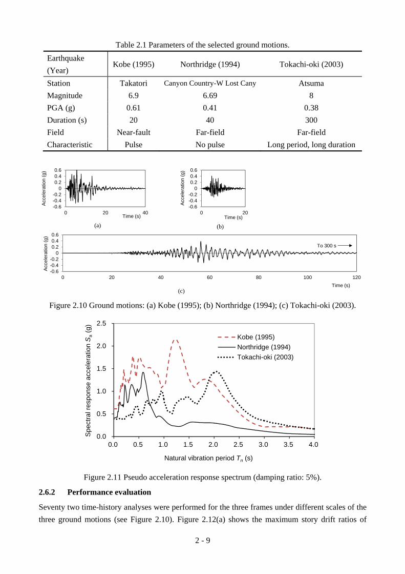
First is the selection of the ground motions for the analysis. The criteria used to the ground motions are: (1) the ground motions should come from popular strong earthquake events, and both the magnitude and intensity should be large; and (2) the selected ground motions should be distinct from each other, so that the analysis can estimate the performance of the structures for different types of ground motions. Three ground motions were chosen from the databases of strong ground motions (Strong-motion Seismograph Networks [8], and PEER Ground Motion Database [9]). The selected ground motions, denoted as Kobe (1995), Northridge (1994) and Tokachi-oki (2003) are shown in Figure 2.10, and their parameters are shown in Table 2.1. The smallest magnitude of the earthquakes is 6.69, and the smallest peak ground acceleration (PAG) is 0.38g. Kobe (1995) is a pulse-type near-fault ground motion, Northridge (1994) is far-field ground motion without pulses, while Tokachi-oki is a long-period long-duration (300 seconds) ground motion.

Second is the scaling of the selected ground motions. The ground motions are scaled by the spectral response acceleration Sa at the fundamental period of the structure. The 5%-damped pseudo acceleration response spectra are shown in Figure 2.11 for the selected ground motions.

Third is the successive increase of the amplitude of the scaled ground motions and time-history analysis for each scale. Each ground motion for the analysis is obtained by adding 20 second of zero-acceleration motion after those in Figure 2.10.

Last is the collection of the structure responses for different scales of ground motions, and comparisons of the responses between the frames.

2 - 9

Table 2.1 Parameters of the selected ground motions. Earthquake (Year)

Kobe (1995) Northridge (1994) Tokachi-oki (2003)

Station Takatori Canyon Country-W Lost Cany Atsuma Magnitude 6.9 6.69 8 PGA (g) 0.61 0.41 0.38 Duration (s) 20 40 300 Field Near-fault Far-field Far-field Characteristic Pulse No pulse Long period, long duration

-0.6-0.4-0.2

00.20.40.6

0 20 40 60 80 100 120

-0.6-0.4-0.2

00.20.40.6

0 20 40-0.6-0.4-0.2

00.20.40.6

0 20Time (s) Time (s)

Time (s)

Acc

eler

atio

n (g

)A

ccel

erat

ion

(g)

Acce

lera

tion

(g)

To 300 s

(a) (b)

(c) Figure 2.10 Ground motions: (a) Kobe (1995); (b) Northridge (1994); (c) Tokachi-oki (2003).

Spec

tral r

espo

nse

acce

lera

tion

Sa

(g)

Natural vibration period Tn (s)

0.0

0.5

1.0

1.5

2.0

2.5

0.0 0.5 1.0 1.5 2.0 2.5 3.0 3.5 4.0

Kobe (1995)Northridge (1994)Tokachi-oki (2003)

Figure 2.11 Pseudo acceleration response spectrum (damping ratio: 5%).

2.6.2 Performance evaluation

Seventy two time-history analyses were performed for the three frames under different scales of the three ground motions (see Figure 2.10). Figure 2.12(a) shows the maximum story drift ratios of

2 - 10

each frame under different scales of Kobe (1995) ground motion, and Figure 2.12(b) the maximum residual story drift ratios. The story drift ratio is defined as the ratio of the story drift to story height, and the maximum story drift ratio is the maximum value for all stories and all the time instants in a time-history analysis. The maximum residual story drift ratio is the maximum story drift ratio at the end of a time-history analysis. The ordinate in Figure 2.12 is the spectral acceleration Sa, which indicates the scales of the selected ground motion. The maximum story drift ratios and residual story drift ratios corresponding to the ground motion of Northridge (1994) is shown in Figure 2.13, and those corresponding to Tokachi-oki (2003) is shown in Figure 2.14. The collapse story drift ratio is set to 0.1, at which the building would collapse or can hardly be repaired. Frame SH-B (strong columns)

Although the maximum strength of Frame SH-B only increase by 7% using much stronger columns, it exhibits significantly smaller maximum story drift and maximum residual story drift for any of the three ground motions than the other frames. The details are below.

In Kobe (1995) ground motion, which is pulse-type, the maximum story drift of Frame SH-B is similar to that of Frame C-B when the spectral acceleration is smaller than 2.0 g, but 50% smaller at the spectral acceleration of 4.0 g. The effect of strong column on reducing the residual deformation is notable, and maximum residual story drift ratio is only 0.0063 in Frame SH-B, which is only about 6% of that of Frame C-B. The collapse spectral acceleration of Frame C-B is about 3.2 g, while that of Frame SH-B increase to 5.0 g, about 56% larger.

In Northridge (1994) ground motion (no pulse), Frame SH-B does not collapse at the spectral acceleration of 9.0 g, while Frame C-B collapses at about 5.0 g. The maximum story drift ratio of Frame SH-B is 40% of that of Frame C-B at the spectral acceleration of 5.0 g, while the maximum residual story drift ratio is 17%.

In the long-duration long-period ground motion Tokachi-oki (2003), the response of the all the frames increases significantly when the spectral acceleration is over 1.0 g. The Frame C-B collapse at 1.4 g, while Frame SH-B at 2.1 g, which is 50% larger than Frame C-B. At the collapse of Frame C-B, the maximum residual story drift of Frame SH-B is 0.0045. Frame H-B (flexible columns)

Although the cross-sectional area of the column in Frame H-B is about 20% smaller than that of Frame C-B, it is shown from the pushover analysis that the roof drift to make the beam yield in Frame H-B is much larger than that in Frame C-B. Compared with Frame C-B, Frame H-B using flexible columns can reduce the residual deformation in all ground motions. The maximum residual story drift is reduced by 60% at the spectral acceleration of 4.0 g in in Kobe (1995) ground motion, and by 60% at 5.0 g in Northridge (1994). The maximum residual story drift ratio in Frame C-B becomes infinite larger at the spectral acceleration of about 1.5 g (collapse), while that in Frame H-B is only 0.03.

2 - 11

0

1

2

3

4

5

0 0.05 0.1 0.15 0.20

1

2

3

4

5

0 0.02 0.04 0.06 0.08 0.1

Spec

tral a

ccel

erat

ion

Sa

(g)

Spe

ctra

l acc

eler

atio

n S a

(g)

Maximum story drift ratio Maximum residual story drift ratio

C-B

H-B

SH-B

C-B

H-B

SH-B

Collapse

(a) (b)

Figure 2.12 Deformation under different scales of spectral accelerations (Kobe (1995)): (a) maximum story drift; (b) residual deformation.

0123456789

10

0 0.05 0.1 0.15 0.20123456789

10

0 0.05 0.1 0.15 0.2

Spec

tral a

ccel

erat

ion

S a(g

)

Spe

ctra

l acc

eler

atio

n S

a(g

)


C-B

H-B

SH-B

C-B

H-B

SH-B

Collapse

(a) (b)

Figure 2.13 Deformation under different scales of spectral accelerations (Northridge (1994)): (a) maximum story drift; (b) residual deformation.

0

0.5

1

1.5

2

2.5

3

0 0.05 0.1 0.15 0.20

0.5

1

1.5

2

2.5

3

0 0.02 0.04 0.06 0.08 0.1

Spec

tral a

ccel

erat

ion

S a(g

)

Spe

ctra

l acc

eler

atio

n S a

(g)


C-B

H-B

SH-B

C-B

H-B

SH-B

Collapse

(a) (b)

Figure 2.14 Deformation under different scales of spectral accelerations (Tokachi-oki (2003)): (a) maximum story drift; (b) residual deformation.

2 - 12

However, the maximum story drift of Frame H-B is not always smaller than Frame C-B. For the no-pulse ground motions, Northridge (1994) and Tokachi-oki (2003), Frame H-B has much smaller maximum story drift ratios (0.06 in Northridge (1994) and 0.05 in Tokachi-oki (2003)), when Frame C-B collapse at the story drift ratio of 0.1. For the pulse-type ground motion, Kobe (1995), Frame H-B has larger maximum story drift ratio than Frame C-B, e.g., about 20% larger when Frame H-B collapses at the spectral acceleration of 3.0 g. Discussion on Prototype frame

Both of the two candidate prototype frames, Frame SH-B and Frame H-B, can reduce the residual deformation. Frame SH-B is superior to reduce the maximum story drift (reduced by 60%) and residual deformation (reduced significantly by 83%~94%). Frame H-B has smaller maximum story drift ratios in the ground motions of Northridge (1994) and Tokachi-oki (2003), but a lager maximum story drift ratio in the ground motion of Kobe (1995). Frame SH-B using strong columns presents a superior and stable performance of minimizing both of the maximum story drift and residual deformation, to make sure of the continuous use of building even after very rare earthquakes, Frame SH-B is adopted as the prototype frame,

2.7 Summary The pattern suitable for the built-up column was proposed, and the seismic performance of the prototype structure was investigated. The main conclusions are as follows:

(1) A bolted built-up column pattern was chosen from eight closed or open sections, using “plate only, bolt only” strategy.

(2) Three braced frames were designed for performance evaluation of the proposed structural system. One is a conventional braced frame, and the other two are the candidate prototype structures using ultra-strength-steel for the columns. One candidate prototype frame used flexible columns with small sections, while the other used strong columns of doubled strength.

(3) Modal analysis was carried out to examine the dynamic characteristics of each case. The three frames exhibited similar modal shapes, but slightly different periods. The first-mode period of the frame with flexible columns is about 15% larger than the conventional frame, while that of the frame with strong columns is basically the same.

(4) Static nonlinear pushover analyses were conducted to investigate the capacity and damage details of the frames using different columns. By using high-strength steel only in the columns, the maximum roof drift to keep the columns and beams elastic can be increased by 57% in the frame using strong columns, and 129% in the frame using flexible columns.

(5) Incremental Dynamic Analysis (IDA) was introduced to evaluate the seismic performance of the frames. The frame using the strong columns is superior to reduce the maximum story drift (cut down by 60%) and residual deformation (cut down significantly by 83% to 94%), while the frame using the flexible columns does not give a stable reduction of the maximum story drift for the pulse-like ground motion and can reduce the residual deformation by 60%. The frame using the strong columns presented a superior and stable capability of

2 - 13

minimizing both the maximum story drift and residual deformation, and was adopted as the prototype structure.

REFERENCES [1] MSC. Software Corporation. MSC (2008). Marc User's Manual (Marc 2008 R1, Volume A,

Theory and user information). Santa Ana, CA 92707, USA. MSC.Software Corporation. [2] MSC. Software Corporation. MSC (2008). Marc User's Manual (Marc 2008 R1, Volume B,

Element Library). Santa Ana, CA 92707, USA. MSC.Software Corporation. [3] Matsumiya T, Suita K, Nakashima M, Liu D, Zhou F, Mizobuchi Y (2005). Effect of RC floor

slab on hysteretic characteristics of steel beams subjected to large cyclic loading. Journal of Structural and Construction Engineering, AIJ, No.598, pp.141-147.

[4] Chopra, AK (2001). Dynamics of Structures, Theory and Applications to Earthquake Engineering. Second Edition, Prentice-Hall, Englewood Cliffs, NJ.

[5] Vamvatsikos D, Cornell CA (2002). Incremental dynamic analysis. Earthquake Engineering and Structural Dynamics, 31: 491–514.

[6] Federal Emergency Management Agency (FEMA) (2000). Recommended Seismic Design Criteria for New Steel Moment-Frame Buildings. FEMA-350, FEMA, Washington, D.C.

[7] Federal Emergency Management Agency (FEMA) (2000). Recommended Seismic Evaluation and Upgrade Criteria for Existing Steel Moment-Frame Buildings. FEMA-351, FEMA, Washington, D.C.

[8] National Research Institute for Earth Science and Disaster Prevention (NIED). Strong-motion Seismograph Networks. (http://www.kyoshin.bosai.go.jp/)

[9] Pacific Earthquake Engineering Research Center. PEER Gound Motion Datobase. (http://peer.berkeley.edu/peer_ground_motion_database/)

2 - 14

3 - 1

CHAPTER 3

Flexural Behavior of Bolted Built-up Columns

Using H-SA700 Steel

3.1 General This chapter reports the first phase of the research on the proposed built-up column using ultra-high strength steel. First, the flexural behavior of the built-up column was investigated by a laboratory testing program where three built-up columns were fabricated and subjected to cyclic loading. Then, the experimental findings are complemented by a finite element simulation study. The experimental and simulation results are used to evaluate its behavior beyond the elastic limit and identify its flexural limit states.

A key design component is the number of bolts used to construct the column. The primary function of the bolts, outside of the connections, is to allow the column to behave as an integrated member. The cross-sectional elements are not continuously connected, so it is not clear how reasonably the integrity of the column is maintained as the column undergoes large deformations. It is cautioned that the bolt pitch defines the unsupported length of the exterior plates. Consequently, the plates are expected to buckle when the column develops large bending moments, with the initiation of buckling dependent primarily on the bolt pitch. Meanwhile, although the column is intended to serve as the elastic member, its behavior beyond the elastic limit needs to be investigated to ensure its intended elastic response and to examine its behavior under extreme loading beyond that specified in codes.

3.2 Test Program

3.2.1 Test specimens

Three column specimens were prepared to examine the flexural performance of the proposed column. Figure 3.1 shows the dimension and bolt arrangement of the specimens. Table 1 lists the three specimens, denoted as H-120, S-120 and H-360, and their properties. Table 2 shows the

3 - 2

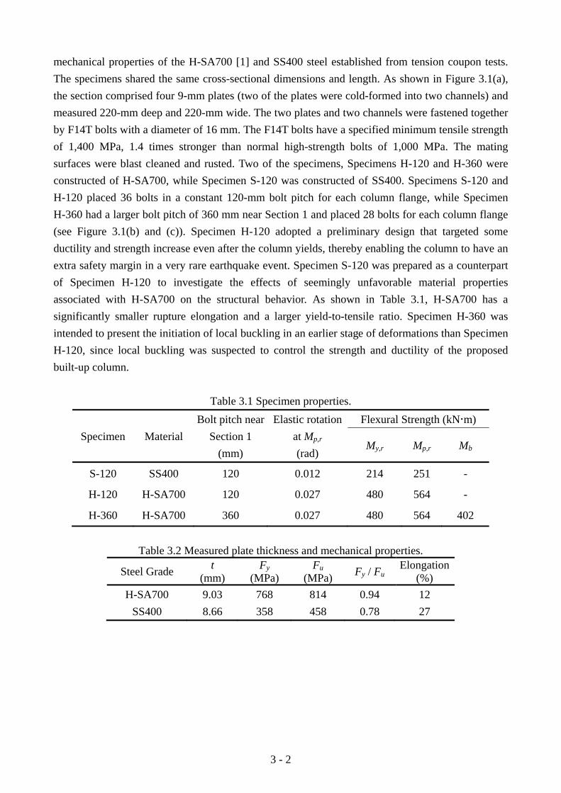
mechanical properties of the H-SA700 [1] and SS400 steel established from tension coupon tests. The specimens shared the same cross-sectional dimensions and length. As shown in Figure 3.1(a), the section comprised four 9-mm plates (two of the plates were cold-formed into two channels) and measured 220-mm deep and 220-mm wide. The two plates and two channels were fastened together by F14T bolts with a diameter of 16 mm. The F14T bolts have a specified minimum tensile strength of 1,400 MPa, 1.4 times stronger than normal high-strength bolts of 1,000 MPa. The mating surfaces were blast cleaned and rusted. Two of the specimens, Specimens H-120 and H-360 were constructed of H-SA700, while Specimen S-120 was constructed of SS400. Specimens S-120 and H-120 placed 36 bolts in a constant 120-mm bolt pitch for each column flange, while Specimen H-360 had a larger bolt pitch of 360 mm near Section 1 and placed 28 bolts for each column flange (see Figure 3.1(b) and (c)). Specimen H-120 adopted a preliminary design that targeted some ductility and strength increase even after the column yields, thereby enabling the column to have an extra safety margin in a very rare earthquake event. Specimen S-120 was prepared as a counterpart of Specimen H-120 to investigate the effects of seemingly unfavorable material properties associated with H-SA700 on the structural behavior. As shown in Table 3.1, H-SA700 has a significantly smaller rupture elongation and a larger yield-to-tensile ratio. Specimen H-360 was intended to present the initiation of local buckling in an earlier stage of deformations than Specimen H-120, since local buckling was suspected to control the strength and ductility of the proposed built-up column.

Table 3.1 Specimen properties.

Specimen Material Bolt pitch near

Section 1 (mm)

Elastic rotation at Mp,r (rad)

Flexural Strength (kN m)

My,r Mp,r Mb

S-120 SS400 120 0.012 214 251 -

H-120 H-SA700 120 0.027 480 564 -

H-360 H-SA700 360 0.027 480 564 402

Table 3.2 Measured plate thickness and mechanical properties.

Steel Grade t (mm)

Fy (MPa)

Fu (MPa) Fy / Fu

Elongation (%)

H-SA700 9.03 768 814 0.94 12 SS400 8.66 358 458 0.78 27

3 - 3

Inside bend radius=18

Top surface of Beam top flange0

12 3

564

Beam

End plate

Column11

220

220

t=9

Centerline of jack

Test length=2450

Section:

11’

2

3

4

56

1 1’

Region for the beam end plate

Region for connecting jack36 49

246

35

8550

5050

50121

121158

10064

14118@

120

12@120

360360

(d) (b) (c)

(a)

Figure 3.1 Details of specimens: (a) column sections; and (b) bolt-hole arrangement in Specimens S-120 and H-120; (c) bolt-hole arrangement in Specimen H-360; and (d) connection (unit: mm).

Table 3.3 lists the limit states and design methods applied to the specimens. Damage was

expected to concentrate at the bottom of the column where key sections were numbered as shown in Figure 3.1(a). The design goal was to achieve a plastic section at a perforated section (limit state 2 in Table 3.3). The key limit states were buckling of the external plate (limit state 3) and slippage between the external plates and internal channels (limit state 7). Both limit states were governed primarily by the bolt pitch. Buckling of the external plate was determined by the elastic column buckling theory, taking each bolt pitch as the column length, and assuming that the ends are fixed against rotation (due to the channels preventing the exterior plates from buckling into the section). The column length of the first bolt pitch between Sections 1 and 3 is the distance between the top edge of the end plate (Section 1’) and Section 3. The critical bolt pitch at which the buckling stress Fb equals the nominal yield strength Fy is 478 mm for SS400 and 283 mm for H-SA700. Specimens S-120 and H-120 met the criteria; hence elastic buckling of the external plate (limit state 3) was to be avoided. Specimen H-360 did not satisfy the criteria, meaning that early buckling was expected. The boundary conditions of the exterior plate within a bolt pitch are rather complex and may not be regarded as completely fixed against rotation. To ensure that no local buckling occurred before yielding, the bolt pitch (120 mm) of Specimen H-120 was chosen in reference to another critical bolt pitch of 142 mm for which the two ends were assumed to be free against rotation. The critical number of bolts needed to avoid plate slippage was computed by assuming a friction coefficient 0.45 between the treated surfaces. The critical number was 9 for SS400 steel and 19 for H-SA700 steel with respect to the shear span of the specimen. Figure 3.1(b) and 3.1(c) show the locations of

3 - 4

18-mm bolt holes in the external plates. All specimens used a sufficient number of bolts to avoid plate slippage (limit state 8).

Table 3.3 Limit states.

# Demand Limit States Design Assumptions

1 Flexure Yielding Yielding initiates at the section that has reduced area due to bolt holes.

2 Flexure Plastic section (target limit state)

Section with bolt holes develops plastic moment.

3 Flexure Buckling of external plate under compression

Stress at critical section acts along unsupported column length. Bolt pitch is taken as column length. Effective length coefficient is 0.5.

4 Flexure Buckling of flanges of interior channels

Width-to-thickness limit for an unsupported edge applies [2,3].

5 Flexure Lateral-torsional buckling of interior channels

Bolt pitch is taken as unsupported beam length [4].

6 Shear Shear yielding and buckling Web of interior channels resist entire shear.

7 Shear Slipping between external plate and channel flanges

Shear between plates is resisted evenly by all bolts within the shear span.

8 Other Bolt failure Standard bolt design applies [5].

Table 3.1 lists key strength values including My,r = Fy Sr, the moment at first yield of sections with bolt holes, Mp,r = Fy Zr, the plastic moment of the section with bolt holes, and Mb = FbS, the moment at which the external plates buckle (applicable only to Specimen H-360). In the above, Fb is the elastic buckling stress of steel plate, S is the elastic section modulus of the gross section, Sr is the elastic section modulus accounting for the bolt holes, and Zr is the plastic section modulus also accounting for the bolt holes.

A concern prior to testing was that the specimen might fracture at the section of the first bolt line and thereby exhibit limited ductility. Assuming that the exterior plate is subjected to uniform tension, the fracture strength at the section reduced due to bolt holes, FuApr, is smaller than the yield strength of the gross section, FyApg, by 11%. Here, Ap,r is the net area of the exterior plate; and Apg is the gross area of the exterior plate. This concern is addressed in a later discussion.

3.2.2 Test setup

Figure 3.2 shows an elevation view of the loading system. A column specimen was connected to two beams at the bottom and to an oil jack at the top. The bottom beam was simply supported at the far end from the specimen. The jack exerted cyclic lateral loading in displacement control. The test length of the column specimen, 2,450 mm, was measured between the loading point and the top face

3 - 5

of the beam top flange. To ensure in-plane bending, the column specimen was laterally supported at two locations, near the loading point and mid-length. Each bottom beam was connected to the column specimen by an extended end-plate [6] as shown in Figure 3.1(d). The dimensions and bolt arrangement of the connection are shown in Figure 3.3. Oversized beams and end plates were used to prevent beam yielding, provide out-of-plane and torsional restraint to the column specimen, and control local limit states of the column specimen. The column-to-beam strength ratio evaluated based on nominal material strengths was 0.34.

1600 1600

2450

2650

1080

950

356

Measured length=720

Roller locations for restraining out-of-plane displacement

150 ton oil jack (Stroke: -210,+290)

H-400x400x13x21

Figure 3.2 Test setup (unit: mm).

140

25220240

140

40050

5050

50 40

140

140

400

400

74126

D=1816

Figure 3.3 Details of beam-to-column connection (unit: mm)

3.2.3 Instrumentations

Figure 3.4 shows the arrangement of displacement transducers. Two displacement transducers, D-1 and D-2, were set within the length of column, 720 mm, measured from the beam top flange. The length of 720 mm was expected to be long enough to cover the portion that present plastic deformation. Five PI displacement transducers, PI-1 to PI-5, were used to monitor possible slippage between the channel flange and the corresponding exterior plate.

3 - 6

Strain gauges were placed extensively in the columns from Sections 1 to 6, as shown in Fig 3.5. The gauges placed in the same section were used to evaluate the section stiffness and confirm whether or not the assumption that plane sections remain plane was valid. The strains obtained from different sections were used to monitor the initiation of yielding in the column, and examine the plastic zone at the column end.

H=7

20

W=110

820

220

PI-1

PI-2 PI-3

PI-4 PI-5

D-1 D-2

Pl displacement transducer

Figure 3.4 Arrangement of displacement transducers

Section 1

Section 2

Section 3

Section 4,5 and 6

Figure 3.5 Arrangement of strain gauges

3.2.4 Test procedure

Cyclic loading was applied according to a prefixed protocol. Two cycles were repeated for drift ratio amplitudes of 0.005, 0.01, 0.02, 0.03, 0.04, 0.06, and 0.08 rad, followed by three cycles between +0.11 and –0.08 rad. The drift is positive when the jack, as viewed in Figure 3.2, pushes the column to the left. The difference between the maximum positive and negative drifts at the last three cycles was due to the stroke limit of the jack. The drift ratio was calculated by dividing the displacement at the loading point by the column test length of 2,450 mm. Testing was continued to the end of the loading protocol or until the load reduced to 70% of the maximum measured value.

3.3 Test Results and Analysis

3 - 7

3.3.1 Behavior

All specimens showed more than 30% reduction in strength from the maximum recorded value by the end of the test. Figure 3.6 shows a photograph of each specimen taken after the test was completed. Figure 3.7 shows the relationship between the moment at Section 1 (see Figure 3.1 and 6) and rotation for each specimen. The moment is estimated as the product of the applied load and the test length, which is the distance between the jack and Section 1 (= 2,350 mm). Rotation θ is evaluated over a length of 720 mm starting at the top face of the beam top flange (see Figure 3.2). Section 1 is located at a distance of 100 mm above the beam top flange. My,test is the measured yield moment, defined as the moment at Section 1 when any of the measured strains at Sections 1 and 2 surpasses the yield strain (0.0017 for SS400 steel and 0.0037 for H-SA700 according to the tensile coupon tests). The instant when local buckling was observed is indicated by a circle mark, and the instant when the moment reached My,test is indicated by a cross mark in Figure 3.7. Table 3.4 summarizes key response parameters including the rotation when My,r was reached, the rotation when local buckling was first observed, and the positive and negative rotations when the strength decreased to 80% of the maximum strength (denoted as θ80). Table 3.4 also lists the measured yield bending moment My,test, maximum recorded moment, Mmax, and the ratio Mmax/Mp,r .

1

5

3

2

3

1’1

5

3

11’

(a) (b) (c)

1

2

3

(d)

Figure 3.6 Specimen after testing: (a) S-120; (b) H-120; (c) H-360; (d) Development of local buckling in H-120.

3 - 8

Table 3.4. Rotation and strength from test results.

Specimen

Rotation (rad) Strength

Yielding Local buckling

Strength decreases to 80% of the

maximum strength

My,test (kN m)

Mmax (kN m) Mmax / Mp,r

H-120 0.022 0.038 +0.067 / –0.090 466 554 +0.98 / –1.03

S-120 0.010 0.029 +0.058 / –0.047 208.0 254 +1.03 / –1.10

H-360 - 0.019 +0.083 / –0.094 - 436 +0.78 / –0.81

-600

-400

-200

0

200

400

600

-0.12 -0.08 -0.04 0 0.04 0.08 0.12

Mom

ent (

kN.m

)

Rotation (rad)

My,r

Mp,r

My,rMp,r

My,test Local buckling

-600

-400

-200

0

200

400

600

-0.12 -0.08 -0.04 0 0.04 0.08 0.12

Mom

ent (

kN.m

)

Rotation (rad)

My,rMp,r

My,r

Mp,rMy,test Local buckling

(a) (b)

-600

-400

-200

0

200

400

600

-0.12 -0.08 -0.04 0 0.04 0.08 0.12

Mom

ent (

kN.m

)

Rotation (rad)

My,rMp,r

My,r

Mp,r

Mb

Mb

Local buckling

(c)

Figure 3.7 Moment-rotation relationship: (a) Specimen S-120; (b) Specimen H-120; and (c) Specimen H-360.

Figure 3.7 indicates many common aspects between the three specimens. All specimens

3 - 9

responded linearly during small rotation cycles. The strength did not increase significantly after exceeding the linear limit. After development of a maximum moment, the strength gradually reduced as the rotation amplitude increased. The gradual strength degradation continued until the end of the test. At rotation cycles exceeding 0.04 rad, the response became increasingly non-symmetric between positive and negative loading. At the end of the test, no fracture was observed.

As the column is intended for use as an elastic member, its behavior and properties in the elastic range are critical. Specimen H-120 had a notably larger yield rotation than S-120, although the SS400 steel for S-120 had a yield strength that was significantly larger than its specified minimum yield strength. Specimen H-120 yielded at a rotation of 0.022 rad when the moment reached My,r , while Specimen S-120 yielded at 0.010 rad, so the elastic deformation capacity was more than doubled by using H-SA700 instead of SS400 steel. Local buckling was observed in the compression-side column flange of Specimen H-120 at about 0.040 rad when the moment reached the maximum strength (see Figure 3.7(b)), while local buckling was observed in Specimen S-120 at about 0.020 rad when the moment was close to its maximum strength (see Figure 3.7(a)). Although the buckling mode was similar between Specimens H-120 and S-120, the rate of strength degradation was notably different. Specimen H-120 reached Mp,r for two cycles at +0.04/ –0.052 rad and subsequently started strength degradation, while Specimen S-120 maintained Mp,r for 5 cycles between ±0.02 and +0.05/ –0.045 rad. This difference in the behavior of strength degradation was attributed in part to the smaller yield ratio associated with H-SA700 and in larger part to the greater force applied to the buckled plate (because of the higher strength) in Specimen H-120.

Specimen H-360 behaved linearly until the moment reached Mb (smaller than My,r) at a rotation of 0.019 rad, which was quite large and close to the elastic deformation capacity of H-120. The moment corresponding to the initiation of the local buckling matched well with the predicted value according to limit state 3 in Table 3.3. When first noted, the local buckling was identified by a small gap that formed suddenly between the exterior plate and the channel on the compression-side column flange between Sections 1’ and 3. Figure 3.7(c) indicates that, as rotation increased, the column maintained a constant moment slightly greater than Mb (see Figure 3.7(c)). While buckling deformation continued to increase in the exterior plates, the inner channels were free of buckling deformation and contributed to the column strength, and thereby avoided immediate decrease in strength.

Two types of local buckling modes occurred in the three specimens. As shown in Figure 3.6(c), the exterior plate buckled out of the section between Sections 1’ and 3 in Specimen H-360 prior to yielding, which was exactly the mode expected in limit state 3. The buckling in Specimens H-120 and S-120 formed after the exterior plates had yielded and, as shown in Figure 3.6(a) and 3.6(b), occurred over a longer length between Sections 1’ and 5, deforming the channel flanges together with the exterior plate. The design target for Specimens H-120 and S-120, which was to achieve the plastic bending moment (limit state 2), was met. Figure 3.6(d) shows how the local buckling deformation progressed in Specimen H-120. The buckling mode was promoted by plastic deformation imposed on the compressed flange as the flange bore against the top corner of the beam end plate. The plastic deformation was not fully corrected when the flange reversed to tension. Eventually, the plastic deformation accumulated into a substantial out-of-straightness that triggered buckling of the

3 - 10

compressed flange.

3.3.2 Elastic stiffness

To monitor the bolt slippage in the column, Pi-gauge displacement transducers were set at Section 3 and another reduced section (820 mm from the beam top flange). Little slippage was observed in Specimen H-360, while in the other two specimens slippage was found at Section 3 after severe local buckling occurred during the ±0.08 rad cycles.

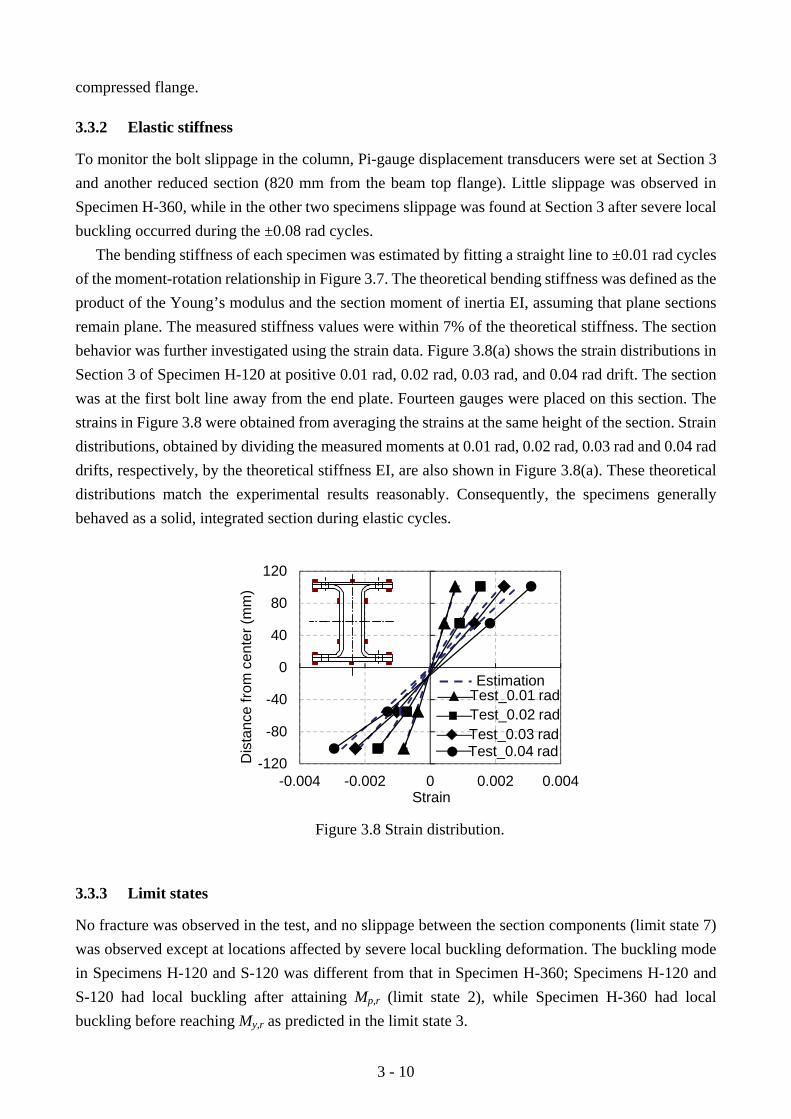
The bending stiffness of each specimen was estimated by fitting a straight line to ±0.01 rad cycles of the moment-rotation relationship in Figure 3.7. The theoretical bending stiffness was defined as the product of the Young’s modulus and the section moment of inertia EI, assuming that plane sections remain plane. The measured stiffness values were within 7% of the theoretical stiffness. The section behavior was further investigated using the strain data. Figure 3.8(a) shows the strain distributions in Section 3 of Specimen H-120 at positive 0.01 rad, 0.02 rad, 0.03 rad, and 0.04 rad drift. The section was at the first bolt line away from the end plate. Fourteen gauges were placed on this section. The strains in Figure 3.8 were obtained from averaging the strains at the same height of the section. Strain distributions, obtained by dividing the measured moments at 0.01 rad, 0.02 rad, 0.03 rad and 0.04 rad drifts, respectively, by the theoretical stiffness EI, are also shown in Figure 3.8(a). These theoretical distributions match the experimental results reasonably. Consequently, the specimens generally behaved as a solid, integrated section during elastic cycles.

-120

-80

-40

0

40

80

120

-0.004 -0.002 0 0.002 0.004

Dis

tanc

e fro

m c

ente

r (m

m)

Strain

Test_0.01 radTest_0.02 radTest_0.03 rad

Estimation

Test_0.04 rad

Figure 3.8 Strain distribution.

3.3.3 Limit states

No fracture was observed in the test, and no slippage between the section components (limit state 7) was observed except at locations affected by severe local buckling deformation. The buckling mode in Specimens H-120 and S-120 was different from that in Specimen H-360; Specimens H-120 and S-120 had local buckling after attaining Mp,r (limit state 2), while Specimen H-360 had local buckling before reaching My,r as predicted in the limit state 3.

3 - 11

Figure 3.7(a) and (b) indicates that the measured yield bending moment My,test and maximum bending moment Mmax (see Table 3.4) were estimated by the yield bending moment My,r and plastic bending moment Mp,r (see Table 3.1) of reduced section accounting for bolt holes (limit states 1 and 2). Figure 3.7(c) shows that the bending moment of Specimen H-360 due to local buckling (408 kN.m) was predicted fairly accurately by Mb (402 kN.m). The maximum yield to strength ratio, which was defined as the ratio of maximum moment Mmax to yield moment My,r , was 1.19 for Specimen H-120, and it was 1.22 for Specimen S-120. Although the difference in the yield ratio was rather significant between H-SA700 and SS400 (Table 3.1), Specimens H-120 and S-120 had a similar rate of increase in strength beyond the yield strength. Specimens H-120 and H-360 developed larger rotation than Specimen S-120 at the same percentage (20%) of strength degradation (see θ80 in Table 3.4). Meanwhile, Figure 3.9 shows the envelope curve established from Figure 3.8. Figure 3.9 offers an alternate view of the cyclic response by normalizing the moment M by Mp,r and normalizing θ by the theoretical elastic rotation when the plastic moment Mp,r is reached, θp. The figure indicates that Specimen H-120 rapidly deteriorated in strength after exceeding θp, while Specimen S-120 maintained Mp up to 6 times θp. For the percentage of strength degradation, Specimen H-120 was deformed to θ80/θp = 2.5 and H-360 to θ80/θp = 3.1 while Specimen S-120 was deformed to θ80/θp = 4.8. The normalized rotation capacity was smaller in Specimen H-120 than in Specimen S-120, partially because of the larger yield ratio of H-SA700 steel, and mainly because of faster strength deterioration due to much larger compressive stress in Specimen H-120. Specimen H-360 exhibited local buckling before yielding, reached the maximum moment at 78% of Mp,r , and had larger rotation capacity than Specimen H-120, because early local buckling reduced the compression force in the flanges of Specimen H-360.

-1.5

-1

-0.5

0

0.5

1

1.5

-5 0 5 10

S-120 H-120 H-360

pθθ /

M/Mp,n

Figure 3.9 Normalized moment versus rotation relationship.

3.3.4 Strain distribution

The strain data from Specimen H-120 was used to study the local strain distribution and progression of yielding. Figure 3.10(a) shows strain values along the center-line of the exterior plates at the

3 - 12

maximum positive loading of the first cycle of 0.02, 0.04, and 0.06 rad. At Section 1, where the exterior plates were connected to the end plates of the beams, the strain at the channel flanges was used. The figure shows, contrary to the conventional concept shown in Figure 3.10(a), that the strains at reduced sections (with bolt holes) were smaller than those at the neighboring cross sections (Sections 2, 4 and 6).

Yield strain

Distance from beam top flange (mm)

Stra

in1(N) 2(G) 3(N) 4(G) 5(N) 6(G)

Section No.

0.02rad0.04rad0.06rad

0.02rad0.04rad0.06rad

Tension side

Compression side

100 200 300 400 500

2.5%

-2.5%

-1.5%

1.5%

-0.5%

0.5%

(a)

0.0%

0.2%

0.4%

0.6%

0.8%

0.02rad 0.04rad 0.06rad

1 2 3

Stra

in Yield strain

Locations on the exterior plate

1 2 3

(b)

Figure 3.10 Strains on the exterior plate of Specimen H-120 (black: tension side; white: compression side): (a) along the centerline; and (b) at Section 3.

Figure 3.10(b) shows the strains of the tension-side exterior plate for three locations of Section 3 at

the maximum positive loading point of the first cycle of 0.02 rad, 0.04 rad and 0.06 rad. The strains distributed uniformly at the cycles of 0.02 rad and 0.04 rad, while the strains at the edges (Locations 1 and 3) became significantly larger than that in the middle (Location 2) at the cycle of 0.06 rad. The strain in Section 2 (no bolt holes) indicated that the strain at center-line was larger than those located at the two edges at the cycle of 0.06 rad. This non-uniform value of local strain distribution was attributed to the influence of concentrated bolt connections. The non-uniform strain distribution exhibited larger strains on the center-line of gross sections and made the sections partially yield,

3 - 13

which might have relieved the strain concentration in the sections with bolt holes and reduced the potential of fractures.

3.4 Finite Element Analysis

3.4.1 Model for Specimen H-120

A numerical study was conducted to complement the experimental findings. The general-purpose software MSC.MARC2008R1 [7] was used to construct nonlinear finite element models. Figure 3.11 shows the finite element model for Specimen H-120. The model was constructed with eight-node, reduced-integration, hexahedral solid elements [8]. One challenge was how to model the large quantity of bolts. The load transfer mechanism between bolted plates depends on whether the plates are in full contact, are separated, or slip against each other. The pretension introduced in the bolts can affect the state of contact and the yielding condition in the vicinity of bolt holes. In this study, the bolts were modeled by pressure acting on mating plates as indicated in Figure 3.11, distributed over an area equal to the size of washers for the total pressure force of 171 kN. Interaction between the mating surfaces was defined by full force transfer in the direction normal to the surface and a friction coefficient of 0.45 in the direction perpendicular to the surface. Figure 3.12 shows the stress versus strain relationships for H-SA700 steel and SS400 steel in terms of both engineering values and true values. The engineering values were obtained from the tensile coupon tests in Table 3.2. True stress versus true strain relationships, which were transformed from the engineering stress versus engineering strain relationships, were used to determine the nonlinear material properties for the models.

Figure 3.13 compares simulated load versus story drift responses for Specimen H-120 against the corresponding test response. The results are shown for two different finite element models using the same meshing scheme. One model, denoted as FEM (mono or cyc), is the adopted model, and the other model, denoted as FEM-NoSlip, has its contact surfaces completely glued to permit no slippage and separation. The curves denoted as FEM (mono) and FEM (cyc) are the responses from monotonic and cyclic loading, respectively. Note that the cyclic analysis stopped due to an intractable convergence problem after reaching the drift ratio of 0.06 rad. It is shown in Figure 3.13 that the proposed model in either monotonic or cyclic loading traces the stiffness and strength of the specimen reasonably up to a drift ratio of 0.06 rad, while FEM-NoSlip model can traces the initial stiffness very well but overestimates the strength at 0.06 rad by 14%, and is hence less adequate. This overestimation was caused mainly by complete composite action between the beam’s end plates and the column flanges, which increased the moment capacity at Section 1 and accordingly changed the most critical section to Section 3. To examine the accuracy of the model for local behavior, experimental strains along the center-line of the exterior plate were compared with those from the adopted model for the drift ratios of 0.04 and 0.06 rad (see Figure 3.14). The strains from the cyclic analysis matched well with the test results at both 0.04 and 0.06 rad. Therefore, the proposed model was able to represent the global and local behavior under cyclic loading until the model stopped due

3 - 14

to the convergence problem, for which complicated contact interactions (slippage, separation, touching) together with the local buckling under cyclic loading were responsible. The difference of local strains between the monotonic and cyclic analysis was small at 0.04 rad, although the strains around Section 2 were smaller in the monotonic analysis at 0.06 rad.

Contact bodies

Face pressure

Bolt model

Lateral displacement load

Figure 3.11 Finite element model.

0

200

400

600

800

0.0 0.1 0.2 0.3

Stre

ss (M

pa)

Strain

H-SA700

SS400

TrueEngineering

H-SA700

SS400

Figure 3.12 Stress versus strain relationships

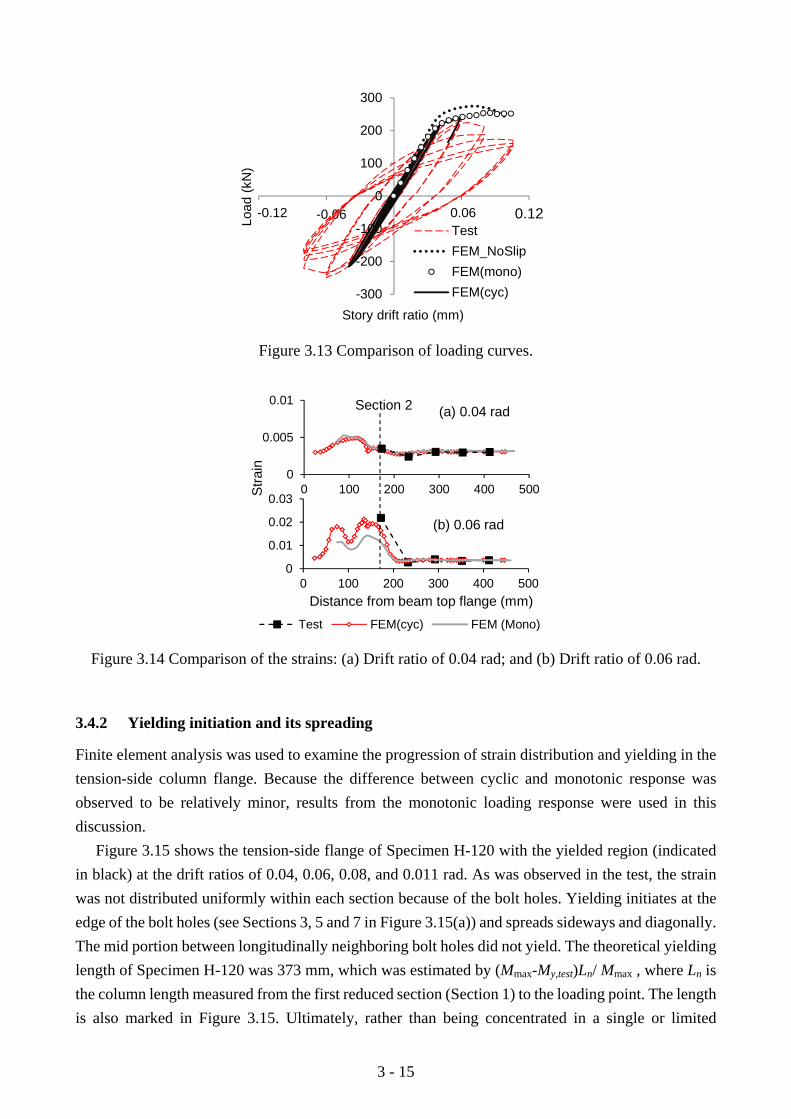
3 - 15

-0.06 0.06 0.12-0.12

-300

-200

-100

0

100

200

300

Load

(kN

)

Story drift ratio (mm)

TestFEM_NoSlipFEM(mono)FEM(cyc)

Figure 3.13 Comparison of loading curves.

0

0.01

0.02

0.03

0 100 200 300 400 500

Test FEM(cyc) FEM (Mono)

0

0.005

0.01

0 100 200 300 400 500


Stra

in

(a) 0.04 rad

(b) 0.06 rad

Section 2

Figure 3.14 Comparison of the strains: (a) Drift ratio of 0.04 rad; and (b) Drift ratio of 0.06 rad.

3.4.2 Yielding initiation and its spreading

Finite element analysis was used to examine the progression of strain distribution and yielding in the tension-side column flange. Because the difference between cyclic and monotonic response was observed to be relatively minor, results from the monotonic loading response were used in this discussion.

Figure 3.15 shows the tension-side flange of Specimen H-120 with the yielded region (indicated in black) at the drift ratios of 0.04, 0.06, 0.08, and 0.011 rad. As was observed in the test, the strain was not distributed uniformly within each section because of the bolt holes. Yielding initiates at the edge of the bolt holes (see Sections 3, 5 and 7 in Figure 3.15(a)) and spreads sideways and diagonally. The mid portion between longitudinally neighboring bolt holes did not yield. The theoretical yielding length of Specimen H-120 was 373 mm, which was estimated by (Mmax-My,test)Ln/ Mmax , where Ln is the column length measured from the first reduced section (Section 1) to the loading point. The length is also marked in Figure 3.15. Ultimately, rather than being concentrated in a single or limited

3 - 16

reduced sections, a continuous yielding zone was formed between Section 1 to Section 7 (see Figure 3.15(c) and (d)). The length of the yielding zone corresponds reasonably well with the theoretical yielding length, meaning that the column would behave like a monolithic column using the reduced section. Besides the local buckling on the compression-side column flange, such extensive yielding would further reduce the fracture potential at reduced sections with bolt holes.

373 mm

234567

Section No.

1

(a) (b) (c) (d)

Figure 3.15 Yielding area at various drift ratios:(a) 0.04 rad; (b) 0.06 rad; (c) 0.08 rad; and (d) 0.11 rad (black: yielding).

Two more cases (shown in Figure 3.16(b) and (c)) were analyzed to further confirm the finding

that a group of reduced sections help enlarge the yielding length of the column. Both are solid sections having the shape of section and material properties identical to those of Specimen H-120. Case H-Hole (see Figure 3.16(b)) has a single row of holes at the column end and is connected to the beams by bolts. Case H-Weld (see Figure 3.16(c)) has no bolt holes and is welded to the beams. In these cases, weld is simulated by perfectly gluing two interacting surfaces. Figure 3.16(a) to (c) show the equivalent plastic strains on the tension-side flanges of the analyzed models at the drift ratio of 0.06 rad. It is shown in Figure 3.16 that the length of yielding zone of H-120 (see Figure 3.16(a)) is similar to H-Weld, which has no bolt holes (see Figure 3.16(c)), and much larger than H-Hole, which has a single row of bolt holes (see Figure 3.16(b)).

3 - 17

0.000

0.0050.0100.0150.0200.0250.030

0.0350.040

(a) (b) (c)

Figure 3.16 Distribution of equivalent plastic strain: (a) H-120; (b) H-Hole; and (c) H-Weld.

3.4.3 Strain concentration

The bolted connection induces strain concentration around the bolt holes, while the welded connections cause significant strain concentration around the weld. Further analysis was presented to compare the mechanism of strain concentrations of the two types of connections.

The significant strain gradient in H-Weld was traced by subdividing the elements of the area around the top edge of the end plate, and the strain gradient at the edge of the bolt hole in H-120 by structural zooming analysis (SZA) [7]. The structural zooming analysis was a procedure to re-compute the local part. A complete re-analysis of the entire model is usually needed to achieve a better evaluation of the local gradients by refining local geometries or reducing element size. Yet, when the local changes have negligible influence on the solution a certain distance away from the changes, it is computationally more efficient to model only the part with the local changes. In the case of H-120 using SZA, the local model was first cut from the global model H-120, specifically, around the bolt hole at Section 1, which was the most critical section. Second, the original elements were subdivided to trace the significant strain gradient. Third, the kinematic boundary conditions of the local model were obtained from the results of the global model. Finally, only the local model was analyzed instead of the entire model. The steps mentioned above were repeated until the strain gradient became stable, and the final mesh is shown in Figure 3.17.

The contours of the longitudinal strain on the tension-side column flanges of H-120 and H-Weld are shown in Figure 3.17 at the story drift ratio of 0.06 rad. The longitudinal direction of the column was defined as the X direction in the figure. It is seen from the strain contours that large strains in H-120 are located on the edge of the bolt holes, especially in the first net section, while the maximum strain in H-Weld is seen around the top edge of the beam end plate. The maximum strain in H-Weld is over 0.04, while that at the edge of the bolt hole in the local model is less than 0.03. Except for the strain concentration around the bolt holes, the strain gradient along the longitudinal direction of H-120 is not as sharp as that of H-Weld.

3 - 18

Area covered by the end plate

Center line of the beam top flange: X=0

X0.0400.0360.0320.0280.0240.0200.0160.0120.0080.0040.000

Strain in the X direction

H-120 H-WeldLocal model

Data points

First net section

Figure 3.17 Strain contour around the column end

0

0.01

0.02

0.03

0.04

0.05

0.06

0 100 200 300 400 500

H-120_center line

H-120_bolt edge

H-Weld_center line

Welded_edge

Top edge of the end plate


Stra

in

H-Weld_edge

Figure 3.18 Strain on the column flange (longitudinal direction)

Figure 3.18 shows the values of longitudinal strains at the critical locations for both of H-120 and

H-Weld. The curves, denoted as “H-120_center line” and “H-120_bolt edge”, show the strains along the center line of the H-120 column and the edge of its bolt hole, respectively. The curves, denoted as “H-Weld_center line” and “H-Weld_ edge”, show the strains along the center line and the longitudinal edge of the H-Weld column, respectively. For H-120, large strains occur at the first net section that is covered by the end plate of the beam. The maximum strain is 0.014 at the center line, and 0.031 around the bolt hole. For H-Weld, large strains occur around the column end, where the column section is enlarged sharply by the end plate. The maximum strain is 0.054 along the edge, and 0.024 along the center line of the column. The maximum strain in H-Weld is 73% larger than that in H-120. The force transferred through bolted connections can be distributed into a larger area, which covers several bolt connectors, and therefore the strain concentration can be mitigated and the rupture risk can be reduced.

3 - 19

3.5 Summary Flexural performance of the proposed bolted built-up column was investigated with both static cyclic tests and finite element simulation. Three specimens, H-120 made of ultra-high strength steel, S-120 made of conventional steel, and H-360 made of ultra-high strength steel with a sparse bolt arrangement, were conducted. Nonlinear finite element analysis was carried out to generalize the findings. The following conclusions were made based on the experiment and finite element analysis:

(1) The elastic bending deformation of the column was more than doubled by using the high-strength steel. The elastic bending stiffness of the bolted built-up column can be estimated based on the assumption that the plane sections remain plane. Slippage was not observed before severe local buckling.

(2) The yield bending moment and maximum bending moment of the built-up column can be estimated reasonably by the yield bending moment and the plastic bending moment of the net area of the section with bolt holes. Specimens H-120 and S-120 had a similar maximum to yield strength ratio of about 1.2, and the ductility was governed primarily by the post-yielding local buckling.

(3) Local buckling was the major factor that induced the deterioration of the column strength, and the elastic local buckling of the exterior plate between two adjacent rows of bolts can be estimated as a plate assuming that its two ends are restrained from rotation.

(4) Although the rupture elongation of H-SA700 was about 12%, it was sufficient to avoid rupture in the specimens up to a story drift ratio of 0.11 rad. The column is planned mainly to remain elastic for its application. Nevertheless, it was able to develop a good deformation capacity, which provides a reasonable safety margin for the design.

(5) A special bolted built-up configuration of the column made it a longer yielding zone because of interaction of a group of reduced sections. Bolted connections exhibited less strain concentration around the column end than welded connections, which further helped the column avoid rupture.

REFERENCES [1] Yoshida Y., Obinata T., Nishio M., Shiwaku T. (2009). Development of high-strength

(780N/mm2) steel for building systems. International Journal of Steel Structures, 9(4): 285-289. [2] Rasmussen K.J.R., Hancock G.J. (1992). Plate slenderness limits for high strength steel sections.

J. Construct. Steel Research, 23:73-96. [3] Ricles J.M., Sause R., Green P.S. (1998). High-strength steel: implications of material and

geometric characteristics on inelastic flexural behavior. Engineering Structures, 20(4-6): 323-335.

[4] American Institute of Steel Construction (AISC) (2010). Specification for structural steel

3 - 20

buildings, ANSI/AISC 360-10, 2010. [5] AIJ (2006). Recommendation for design of connections in steel structures. The Architectural

Institute of Japan, 2006. [6] American Institute of Steel Construction (AISC) (2003). Extended End-Plate Moment

Connections (Seismic and Wind Applications), Second Edition, 2003. [7] MSC. Software Corporation. MSC (2008). Marc User's Manual (Marc 2008 R1, Volume A,


Element Library). Santa Ana, CA 92707, USA. MSC.Software Corporation.

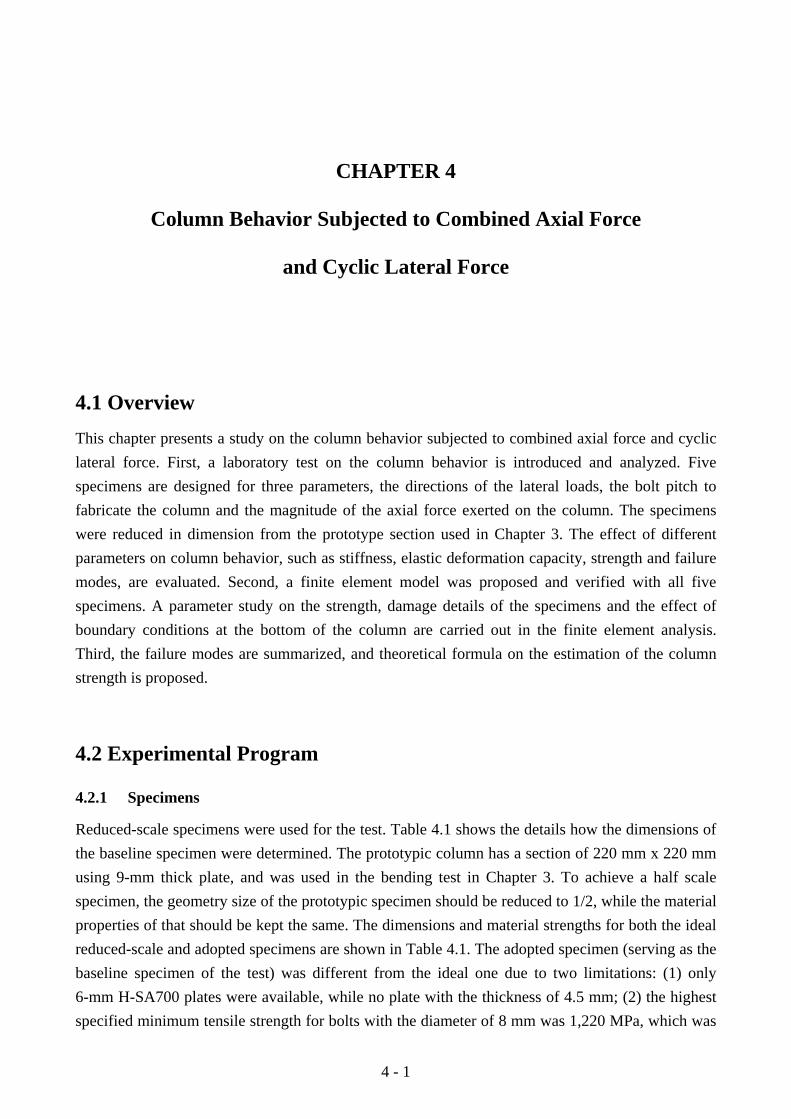
4 - 1

CHAPTER 4

Column Behavior Subjected to Combined Axial Force

and Cyclic Lateral Force

4.1 Overview This chapter presents a study on the column behavior subjected to combined axial force and cyclic lateral force. First, a laboratory test on the column behavior is introduced and analyzed. Five specimens are designed for three parameters, the directions of the lateral loads, the bolt pitch to fabricate the column and the magnitude of the axial force exerted on the column. The specimens were reduced in dimension from the prototype section used in Chapter 3. The effect of different parameters on column behavior, such as stiffness, elastic deformation capacity, strength and failure modes, are evaluated. Second, a finite element model was proposed and verified with all five specimens. A parameter study on the strength, damage details of the specimens and the effect of boundary conditions at the bottom of the column are carried out in the finite element analysis. Third, the failure modes are summarized, and theoretical formula on the estimation of the column strength is proposed.

4.2 Experimental Program

4.2.1 Specimens

Reduced-scale specimens were used for the test. Table 4.1 shows the details how the dimensions of the baseline specimen were determined. The prototypic column has a section of 220 mm x 220 mm using 9-mm thick plate, and was used in the bending test in Chapter 3. To achieve a half scale specimen, the geometry size of the prototypic specimen should be reduced to 1/2, while the material properties of that should be kept the same. The dimensions and material strengths for both the ideal reduced-scale and adopted specimens are shown in Table 4.1. The adopted specimen (serving as the baseline specimen of the test) was different from the ideal one due to two limitations: (1) only 6-mm H-SA700 plates were available, while no plate with the thickness of 4.5 mm; (2) the highest specified minimum tensile strength for bolts with the diameter of 8 mm was 1,220 MPa, which was

4 - 2

smaller than the strength of bolts (1400 MPa) used in the prototypic column. The first limitation would increase the resistance against local buckling, and the second would induce earlier failure of bolts.

Table 4.1 Size of the specimen

Section (mm x mm)

Prototype

Ideal specimen

Adopted specimen

220x220 110x110 110x110 Shear span (mm) 2450 1225 1230

Plate (mm) Thickness 9 4.5 6 Bend radius 27 13.5 18

Bolt (mm) Diameter 16 8 8 Pitch 120 60 60

Tensile Strength (MPa)

Plate 780 780 780 Bolt 1,400 1,400 1,220

Table 4.2 lists the parameters for each specimen, and Figure 4.1 shows the details of specimens.

Five specimens with the same section of 110 mm × 110 mm were constructed for different parameters. The column consists of two plates and two cold-formed channels, and is built using high-strength bolts. The bolts had a nominal diameter of 8 mm and a specified minimum tensile strength of 1,220 MPa. Since the column was intended for use in the elastic range, the elastic deformation capacity, elastic stiffness, and the safety margin above the elastic limit were the main concerns for specimen design. Three parameters were chosen, and they were lateral load direction (about the strong or weak axis, bolt pitch of 60 mm or 120 mm near the critical section, and axial force ratio of 0.0, 0.2 or 0.4. The axial force ratio was defined as the ratio of the axial compressive force to the axial compressive yield strength of the gross cross-sectional area. The baseline specimen (denoted as X60N2) was loaded about the strong axis (X-axis), and had a bolt pitch of 60 mm and an axial force ratio of 0.2. A larger bolt pitch may cause an early local buckling, and hence reduce the strength of the column, while a larger axial force may affect the stiffness, strength, and yield rotation. The exterior plate of the flange between two adjacent reduced sections was more critical to buckling. It is shown from the bending test in Chapter 3 that the buckling of the exterior plate can be reasonably estimated by the elastic column buckling theory, taking each bolt pitch as the column length, and assuming that the ends are fixed against rotation (the channels prevent the exterior plates from buckling into the section). The critical stress for the local buckling of the

4 - 3

exterior plate was 1,684 MPa for the specimen with a bolt pitch of 60 mm, and 6,737 MPa for specimens with a bolt pitch of 120 mm; the specimens were expected not to sustain local buckling of the exterior plate before yielding. The material properties of the steel plates used for the specimens are shown in Table 4.3. The H-SA700 steel had a rupture elongation of about 13%, which is only half of that of conventional mild steel, and a yield ratio (the ratio of the yield stress to tensile stress) of 0.94, which suggests a limited strength increase beyond the yield stress.

P=60P=120 P=60

N/N0=0.2

About X axis About Y axis

N/N0=0.0, 0.2, 0.4 N/N0=0.2

110x110

X

Y

X60N2 X120N2 Y60N2X60N0 X60N4

Stiffener

P=60

Section

Top plate

Bottom plate

(a) (b) (c)

Figure 4.1 Specimens: (a) X60N0, X60N2, X60N4; (b) X120N2; (c) Y60N2.

Table 4.2 Parameters for specimens Specimen

No. Load

direction Bolt

pitch(mm) Axial force ratio

N/N0 Instructions

X60N0 X 60 0.0 No axial force X60N2 X 60 0.2 Baseline Specimen X60N4 X 60 0.4 Larger axial force X120N2 X 120 0.2 Larger bolt pitch Y60N2 Y 60 0.2 Different load direction

Table 4.3 Material Properties

Specimen No. Thickness

(mm) Yield Stress

Fy (MPa) Tensile Stress

Fmax (MPa) Yield Ratio

Fy/Fmax Rupture

Elongation X60N0, X60N2, X60N4, X120N2

6.0 803 851 0.94 13%

Y60N2 6.0 787 833 0.94 13%

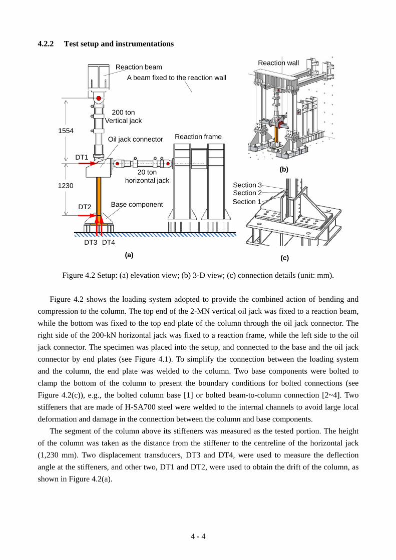
4 - 4

4.2.2 Test setup and instrumentations

1230

1554Reaction frame

200 ton Vertical jack

20 ton horizontal jack

Base component

A beam fixed to the reaction wall

DT1

DT2

DT3 DT4

Reaction beam

Oil jack connector

Reaction wall

(a)

(b)

(c)

Section 1Section 2Section 3

Figure 4.2 Setup: (a) elevation view; (b) 3-D view; (c) connection details (unit: mm).

Figure 4.2 shows the loading system adopted to provide the combined action of bending and

compression to the column. The top end of the 2-MN vertical oil jack was fixed to a reaction beam, while the bottom was fixed to the top end plate of the column through the oil jack connector. The right side of the 200-kN horizontal jack was fixed to a reaction frame, while the left side to the oil jack connector. The specimen was placed into the setup, and connected to the base and the oil jack connector by end plates (see Figure 4.1). To simplify the connection between the loading system and the column, the end plate was welded to the column. Two base components were bolted to clamp the bottom of the column to present the boundary conditions for bolted connections (see Figure 4.2(c)), e.g., the bolted column base [1] or bolted beam-to-column connection [2~4]. Two stiffeners that are made of H-SA700 steel were welded to the internal channels to avoid large local deformation and damage in the connection between the column and base components.

The segment of the column above its stiffeners was measured as the tested portion. The height of the column was taken as the distance from the stiffener to the centreline of the horizontal jack (1,230 mm). Two displacement transducers, DT3 and DT4, were used to measure the deflection angle at the stiffeners, and other two, DT1 and DT2, were used to obtain the drift of the column, as shown in Figure 4.2(a).

4 - 5

4.2.3 Loading protocol

Cyclic loading was applied to all the columns. The loading protocol for the lateral drift of the column was as follows: two cycles for each story drift ratio (called as SDR hereafter) of ±0.005, ±0.01, ±0.02, ±0.03, ±0.04, ±0.06, ±0.08 rad and finally three cycles of ±0.10 rad, as shown in Figure 4.3. The story drift ratio here is defined as the ratio of the drift to the column height. The loading was terminated when severe local buckling or rupture in the column occurred.

Story drift ratio (rad)

Number of cycles2 2 2 2 2 2 2 3

-0.1

0.1

0.005 0.01 0.02 0.03 0.04 0.060.08

0.1

Figure 4.3 Loading protocol

4.3 Analysis of Test Results Figure 4.4 shows the moment versus rotation relationship for each specimen. The moment uses the bending moment of the column at the first reduced section from the stiffener (Section 1 in Figure 4.2(c)), which was expected as the most critical section to yielding and rupture. The column rotation was obtained by subtracting the deflection angle of the bottom stiffeners from the story drift angle of the column. Three types of markers were used to indicate the instants when local buckling, plate fracture, or bolt fracture was observed. Figure 4.5 presents the photos for the final failure state of each specimen. The arrows in the photos indicate the locations where fracture occurred.

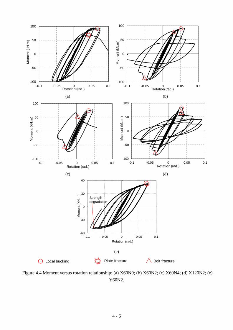
4 - 6

-100

-50

0

50

100

-0.1 -0.05 0 0.05 0.1

Mom

ent (

kN.m

)

Rotation (rad.)

-100

-50

0

50

100

-0.1 -0.05 0 0.05 0.1

Mom

ent (

kN.m

)

Rotation (rad.) (a) (b)

-100

-50

0

50

100

-0.1 -0.05 0 0.05 0.1

Mom

ent (

kN.m

)

Rotation (rad.)

-100

-50

0

50

100

-0.1 -0.05 0 0.05 0.1

Mom

ent (

kN.m

)

Rotation (rad.) (c) (d)

-60

-30

0

30

60

-0.1 -0.05 0 0.05 0.1

Mom

ent (

kN.m

)

Rotation (rad.)

Strength degradation

(e)

Local bucking Plate fracture Bolt fracture

Figure 4.4 Moment versus rotation relationship: (a) X60N0; (b) X60N2; (c) X60N4; (d) X120N2; (e) Y60N2.

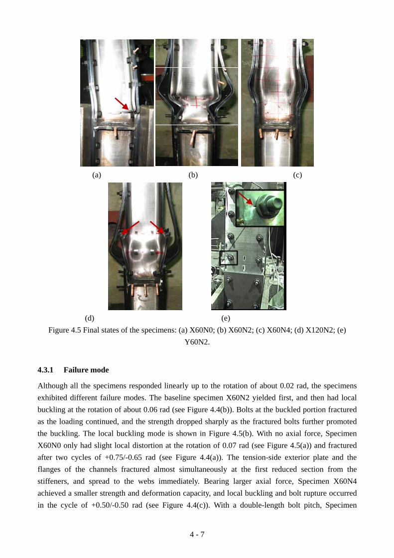
4 - 7

(a) (b) (c)

(d) (e)

Figure 4.5 Final states of the specimens: (a) X60N0; (b) X60N2; (c) X60N4; (d) X120N2; (e) Y60N2.

4.3.1 Failure mode

Although all the specimens responded linearly up to the rotation of about 0.02 rad, the specimens exhibited different failure modes. The baseline specimen X60N2 yielded first, and then had local buckling at the rotation of about 0.06 rad (see Figure 4.4(b)). Bolts at the buckled portion fractured as the loading continued, and the strength dropped sharply as the fractured bolts further promoted the buckling. The local buckling mode is shown in Figure 4.5(b). With no axial force, Specimen X60N0 only had slight local distortion at the rotation of 0.07 rad (see Figure 4.5(a)) and fractured after two cycles of +0.75/-0.65 rad (see Figure 4.4(a)). The tension-side exterior plate and the flanges of the channels fractured almost simultaneously at the first reduced section from the stiffeners, and spread to the webs immediately. Bearing larger axial force, Specimen X60N4 achieved a smaller strength and deformation capacity, and local buckling and bolt rupture occurred in the cycle of +0.50/-0.50 rad (see Figure 4.4(c)). With a double-length bolt pitch, Specimen

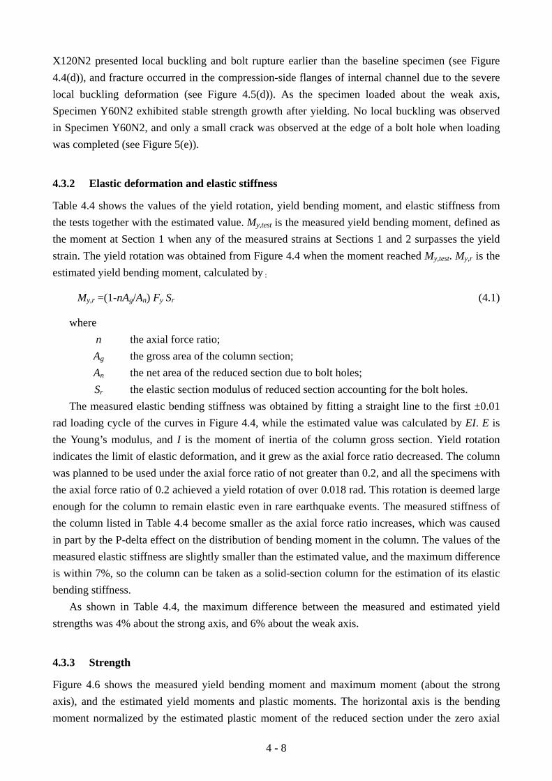
4 - 8

X120N2 presented local buckling and bolt rupture earlier than the baseline specimen (see Figure 4.4(d)), and fracture occurred in the compression-side flanges of internal channel due to the severe local buckling deformation (see Figure 4.5(d)). As the specimen loaded about the weak axis, Specimen Y60N2 exhibited stable strength growth after yielding. No local buckling was observed in Specimen Y60N2, and only a small crack was observed at the edge of a bolt hole when loading was completed (see Figure 5(e)).

4.3.2 Elastic deformation and elastic stiffness

Table 4.4 shows the values of the yield rotation, yield bending moment, and elastic stiffness from the tests together with the estimated value. My,test is the measured yield bending moment, defined as the moment at Section 1 when any of the measured strains at Sections 1 and 2 surpasses the yield strain. The yield rotation was obtained from Figure 4.4 when the moment reached My,test. My,r is the estimated yield bending moment, calculated by :

My,r =(1-nAg/An) Fy Sr (4.1)

where n the axial force ratio; Ag the gross area of the column section; An the net area of the reduced section due to bolt holes; Sr the elastic section modulus of reduced section accounting for the bolt holes.

The measured elastic bending stiffness was obtained by fitting a straight line to the first ±0.01 rad loading cycle of the curves in Figure 4.4, while the estimated value was calculated by EI. E is the Young’s modulus, and I is the moment of inertia of the column gross section. Yield rotation indicates the limit of elastic deformation, and it grew as the axial force ratio decreased. The column was planned to be used under the axial force ratio of not greater than 0.2, and all the specimens with the axial force ratio of 0.2 achieved a yield rotation of over 0.018 rad. This rotation is deemed large enough for the column to remain elastic even in rare earthquake events. The measured stiffness of the column listed in Table 4.4 become smaller as the axial force ratio increases, which was caused in part by the P-delta effect on the distribution of bending moment in the column. The values of the measured elastic stiffness are slightly smaller than the estimated value, and the maximum difference is within 7%, so the column can be taken as a solid-section column for the estimation of its elastic bending stiffness.

As shown in Table 4.4, the maximum difference between the measured and estimated yield strengths was 4% about the strong axis, and 6% about the weak axis.

4.3.3 Strength

Figure 4.6 shows the measured yield bending moment and maximum moment (about the strong axis), and the estimated yield moments and plastic moments. The horizontal axis is the bending moment normalized by the estimated plastic moment of the reduced section under the zero axial

4 - 9

force, while the vertical axis is the axial force ratio. The solid and hollow markers (square or triangle) indicate the measured yield moment and maximum moment, respectively. The lines show the estimated values with respect to the net area of the reduced section and gross area of the full section. The estimated plastic moment under any given axial force was calculated assuming that all fibers in the reduced section reached measured yield stress Fy, either in tension or compression. The distribution of the fibers in the section for calculation is shown in Figure 4.7. The yield strength was inversely proportional to the magnitude of the axial force, and also as shown in Table 3, the estimated yield strength of the reduced section matched well with its corresponding measured values. The estimated yield strength can be used to identify the limit of elastic range.

Table 4.4 Test results and estimations

Specimen No.

N/N0 Yield rot.

(rad)

Bending moment (kN.m) Elastic stiffness EI (kN.m2)

My,test My,r My,test/My,r Test Est. Test/Est.

X60N0 0.0 0.029 69.6 72.4 0.96 1.201×103 1.230×103 0.98 X60N2 0.2 0.021 55.5 55.3 1.00 1.165×103 1.230×103 0.95 X60N4 0.4 0.014 39.1 38.3 1.02 1.149×103 1.230×103 0.93 X120N2 0.2 0.021 54.8 55.3 0.99 1.181×103 1.230×103 0.96 Y60N2 0.2 0.018 27.0 25.4 1.06 0.564×103 0.590×103 0.96

M/Mp,r

N/N

0

0

0.2

0.4

0.6

0.8

1

0.0 0.2 0.4 0.6 0.8 1.0 1.2

Plastic (Est. Gross) Yield (Est.Gross)Yield (Est.Net) Plasitc (Est.Net)Yield (Test, pitch=60) Max (Test, pitch=60)Yield (Test, pitch=120) Max (Test, pitch=120)

Figure 4.6 Yield strength and maximum strength (about the strong axis).

4 - 10

No fiber

(a) (b)

Figure 4.7 Fibers of the section: (a) gross section; (b) reduced section.

The design goal was to achieve the plastic moment of the reduced section. The maximum moments of all tests exceeded the estimated plastic moment of the reduced section, although none of them reached the plastic moment of the gross section. The amount of the overstrength from the plastic moment of the reduced section varied among specimens. As shown in Figure 4.6, the specimen with a smaller bolt pitch achieved a larger maximum strength, e.g., the specimens under the axial force ratio of 0.2. When the axial force ratio equalled to zero, the overstrength was caused mainly by the stress hardening of the material after yielding, and the maximum strength was limited by the fracture of the tension-side flange. As the axial force ratio increased, the overstrength became larger. The overstrength was not only caused by the stress hardening but also by the reason that the compressive resistance of the flange was not simply governed by the reduced section. Because the maximum strength was limited by the reduced section when axial force was small, the estimated plastic moment of the gross section overestimated the bending moment under small axial force ratios, e.g., more than 10% larger when axial force is 0.0.

For the loading about the weak axis, Specimen Y60N2 yielded at the moment of 27.0 kN.m and increased to its maximum moment of 53.3kN.m, which was almost twice the yield moment. The larger strength increase about the weak axis was due to the shape effect of the section. It can be seen from Figure 4.4(e) that the strength about weak axis was not completely independent of loading directions (positive direction or negative direction, the positive direction was the pushing direction of the horizontal jack in Figure 4.2(a)), and strength degradation was observed at the rotation of about -0.08 rad when the same loading cycle was repeated (the location was indicated in Figure 4.4(e)). Such strength degradation was not observed at the positive loading direction, and the strength kept increasing. The strength difference between the negative-direction loading and positive-direction loading was caused by the inherent asymmetry attached with the loading protocol. One side of column flanges always experienced larger tensile deformation first, while the other side experienced larger compressive deformation first.

4 - 11

4.4 Finite Element Model and Parameter Study

4.4.1 Modeling

Finite element analysis was carried out to complement the experimental findings, and the general-purpose software MSC.MARC2008R1 [5] was used to construct nonlinear finite element models. Figure 4.8 shows the finite element model for the baseline specimen (Specimen X60N2). The entire model was constructed with the same type of elements, the eight-node 3-D first-order hexahedral solid elements (Element No.117 in the element library, which is preferred over higher-order elements when used in a contact analysis [6]). Rigid links were used to connect the top end plate of the column and the bottom pin of the vertical jack (the pin located at the center line of the horizontal jack). Six degrees of freedom were fixed completely at the bottom of the model, and the axial force and lateral displacement were exerted on the top end of the model (see Figure 4.8(a)). One challenge was how to model the large quantity of bolted connections. In Chapter 3, the action of bolts was simulated by equivalent pressure force, distributed over an area equal to the size of washers. Yet as mentioned in Chapter 4.2, the thickness of the plate in the half scale specimen was not exactly reduced by 50%, and the bent radius was enlarged with the thickness of the plate, so qualified element meshing cannot be achieved at the narrow area between the washer area and the bent portion of the channel. Hence, bolts were modeled explicitly (see Figure 4.8(b)) and the pretension forces were simulated by setting initial stress in the bolts. Contact was set between all the components, including bolt, nuts, plates and channels. Interaction between the mating surfaces was treated as full force transfer in the direction normal to the surface and a friction coefficient was set to 0.25 (the surface was clean and not being processed) in the direction perpendicular to the surface. The material properties listed in Table 4.3 were used to determine the nonlinear material properties for the model, which was the same as the one used in Chapter 3.4. A tri-linear stress strain relationship was utilized for the bolts [7, 8], as shown in Figure 4.9. The bolt yield stress, Fyb, is 1,100 MPa, and the tensile strength, Fub, was 1,220 MPa. The same loading protocol in Chapter 4.2.3 was used for all the cases in the analysis.

4 - 12

Bolt with pretension

Rigid bottom

Solid element

N

Rigid link (Jack head)

Displacement load

(c)

Base

Column

(b)

Half model

Stiffener

Restraint for symmetric

(a)

Figure 4.8 Finite element model: (a) elevation view; (b) local view; (c) plane view.

E

Fub

Fyb

Strain εεy 3.5 εy

Stress σ

Fub = 1,220 MPa

Fyb = 1,100 MPa

E = 205 GPa

εy = 0.00537

Figure 4.9 Stress-strain relationship for high-strength bolt

4 - 13

4.4.2 Verification

Proposed model for baseline specimen (X60N2) The proposed model was used to represent the behavior of the specimens. Figure 4.10 shows the comparison of the column moment versus rotation relationships of the baseline specimen (X60N2) from both the finite element analysis and test. The proposed model reasonably represents the stiffness, maximum strength, and strength deterioration caused by local buckling. The finial deformation modes, which were caused by severe yielding and local buckling, were also compared with the pictures in Figure 4.10. They also matched well with each other. Although the strength dropped slightly each time when a bolt ruptured, the strength deterioration was primarily dominated by the post-yield local buckling, and bolt rupture did not influence significantly on subsequent cycles of the moment versus rotation relationship curve.

-120

-80

-40

0

40

80

120

-0.12 -0.08 -0.04 0.00 0.04 0.08 0.12

FEM

Test

Mom

ent (

kN.m

)

Rotation (rad.)

Test FEM

Figure 4.10 Comparison between the test results and finite element analysis (Specimen X60N2)

Simple model

Besides the proposed model, a simple model was also tried to seek possible ways of reducing the work of modeling and the effort of computation. In the simple model, bolted connections and the contact interaction between two plates were simplified by gluing two plates (no slippage and separation). Figure 4.11 shows the moment versus rotation relationships obtained from the analysis of the simple model (denoted as FEM_simple) and the test results. The simple model exhibited larger maximum strength, larger stiffness under large cycles, and smaller strength deterioration. The simple model failed to give a good simulation on the local buckling of the column flanges, which determined the maximum strength, significantly affected the strength deterioration and caused pinching of the test curve in Figure 4.11. To achieve sufficient accuracy of the analysis, the proposed model was adopted to for further verification and parameter study.

4 - 14

-120

-80

-40

0

40

80

120

-0.12 -0.08 -0.04 0.00 0.04 0.08 0.12

FEM_simpleTest

Rotation (rad.)

Mom

ent (

kN.m

)

Figure 4.11 Comparison of moment versus rotation relationship (Specimen X60N2)

Verification by other four specimens

By changing the axial force of the proposed model for the baseline specimen, the numerical models to represent the behavior of Specimens X60N0 and X60N4 were obtained. The model for Specimen X120N2 was obtained by enlarging the bolt pitch, and the model for Specimen Y60N2 by rotating the column by 90 degree and using the material properties for Specimen Y60N2 in Table 4.3. The same contact properties and material model were used in all the models. Figure 4.12 to 4.15 show the comparisons of the simulation results and test results for Specimens X60N0, X60N4, X120N2 and Y60N2, respectively.

-120

-80

-40

0

40

80

120

-0.12 -0.08 -0.04 0.00 0.04 0.08 0.12

Test

FEM

Test

FEM

Mom

ent (

kN.m

)

Rotation (rad)

Figure 4.12 Comparison between test results and finite element analysis (Specimen X60N0) As for Specimen X60N0, the model simulated its strength and stiffness quite well until rupture

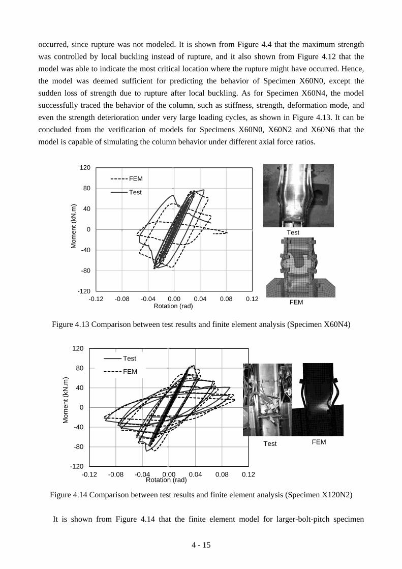
4 - 15

occurred, since rupture was not modeled. It is shown from Figure 4.4 that the maximum strength was controlled by local buckling instead of rupture, and it also shown from Figure 4.12 that the model was able to indicate the most critical location where the rupture might have occurred. Hence, the model was deemed sufficient for predicting the behavior of Specimen X60N0, except the sudden loss of strength due to rupture after local buckling. As for Specimen X60N4, the model successfully traced the behavior of the column, such as stiffness, strength, deformation mode, and even the strength deterioration under very large loading cycles, as shown in Figure 4.13. It can be concluded from the verification of models for Specimens X60N0, X60N2 and X60N6 that the model is capable of simulating the column behavior under different axial force ratios.

-120

-80

-40

0

40

80

120

-0.12 -0.08 -0.04 0.00 0.04 0.08 0.12

FEM

Test

Test

FEM

Mom

ent (

kN.m

)

Rotation (rad)

Figure 4.13 Comparison between test results and finite element analysis (Specimen X60N4)

Test FEM

-120

-80

-40

0

40

80

120

-0.12 -0.08 -0.04 0.00 0.04 0.08 0.12

Test

FEM

Mom

ent (

kN.m

)

Rotation (rad)

Figure 4.14 Comparison between test results and finite element analysis (Specimen X120N2)

It is shown from Figure 4.14 that the finite element model for larger-bolt-pitch specimen

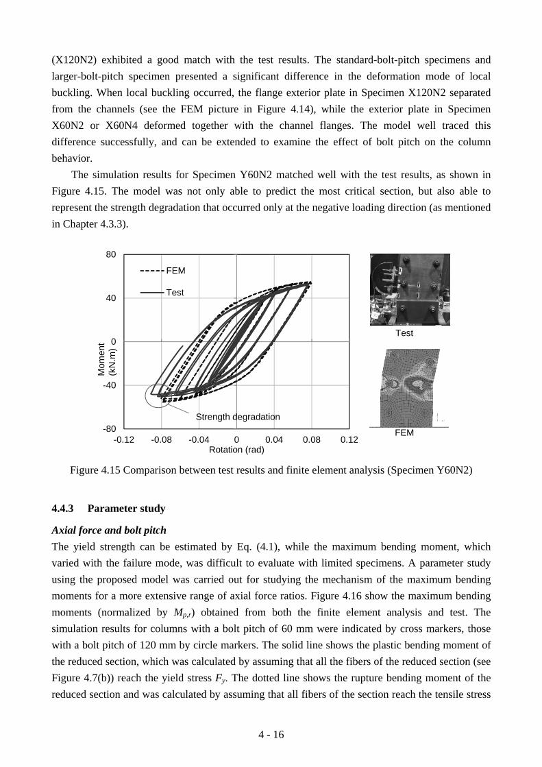
4 - 16

(X120N2) exhibited a good match with the test results. The standard-bolt-pitch specimens and larger-bolt-pitch specimen presented a significant difference in the deformation mode of local buckling. When local buckling occurred, the flange exterior plate in Specimen X120N2 separated from the channels (see the FEM picture in Figure 4.14), while the exterior plate in Specimen X60N2 or X60N4 deformed together with the channel flanges. The model well traced this difference successfully, and can be extended to examine the effect of bolt pitch on the column behavior.

The simulation results for Specimen Y60N2 matched well with the test results, as shown in Figure 4.15. The model was not only able to predict the most critical section, but also able to represent the strength degradation that occurred only at the negative loading direction (as mentioned in Chapter 4.3.3).

-80

-40

0

40

80

-0.12 -0.08 -0.04 0 0.04 0.08 0.12

FEM

Test

Mom

ent

(kN

.m)

Rotation (rad)

Test

FEM

Strength degradation

Figure 4.15 Comparison between test results and finite element analysis (Specimen Y60N2)

4.4.3 Parameter study

Axial force and bolt pitch The yield strength can be estimated by Eq. (4.1), while the maximum bending moment, which varied with the failure mode, was difficult to evaluate with limited specimens. A parameter study using the proposed model was carried out for studying the mechanism of the maximum bending moments for a more extensive range of axial force ratios. Figure 4.16 show the maximum bending moments (normalized by Mp,r) obtained from both the finite element analysis and test. The simulation results for columns with a bolt pitch of 60 mm were indicated by cross markers, those with a bolt pitch of 120 mm by circle markers. The solid line shows the plastic bending moment of the reduced section, which was calculated by assuming that all the fibers of the reduced section (see Figure 4.7(b)) reach the yield stress Fy. The dotted line shows the rupture bending moment of the reduced section and was calculated by assuming that all fibers of the section reach the tensile stress

4 - 17

Fu.

Either of cross markers and cycle markers exhibited a distribution that was almost parallel to

the estimated line for either of rupture moment and plastic moment, which confirmed experimental

conclusion that the maximum bending strength was dominated by behavior of the reduced section.

When the axial force was small (e.g., the axial force ratio was smaller than 0.1), the maximum

moment was limited by the tensile strength of the column flange. When axial force became larger,

the local buckling of the column flange became more critical, and the maximum moment was

limited by the compression strength of the column. Based on these two different mechanisms to

form the maximum moment, the axial force ratio versus maximum bending moment relationship

can be simplified approximately by two straight lines, one for small axial force ratios and the other

for large axial force ratios. The two pieces of solid lines in Figure 4.16 was shown as an illustration

of simplification for the column with a bolt pitch of 120 mm.

0

0.2

0.4

0.6

0.8

1

1.2

0 0.2 0.4 0.6 0.8 1 1.2

Plasitc (Est.) Rupture (Est.) Up bound (Est.) Max (pitch=60)

Max (pitch=120) FEM (pitch=60) FEM (pitch=120)

M/Mp,r

N/N

0

Concept curve

No fiberN

M

-Fu

+Fu

Up bound

Figure 4.16 Axial force ratio versus maximum bending moment

The maximum strength was significantly affected by the bolt pitch. The maximum strength of

the larger-bolt-pitch (120 mm) column was larger than the plastic moment, and closed to the rupture

moment, while that of the column with a smaller bolt pitch (60-mm) was larger than the

corresponding rupture moment. It was against the conventional understanding that the column

achieved a maximum moment larger than its rupture moment. Although the resistance of

tension-side column flange cannot go beyond its rupture strength of the net area accounting bolt

holes, the resistance of the compression-side column flange was not limited to its reduced area.

4 - 18

When the reduced section yields due to compression, the bolt hole deforms and the bolted

connections participate in the compression of the flange to some extent. An upper bound estimated

moment can be achieved using the tensile stress Fu for all the fibers in the section, and neglecting

the reduction of bolt holes and local buckling in the compressive flange (see the curve for upper

bound moment in Figure 4.16 is denoted as “up bound”). The maximum moments of the column

with the bolt pitch of 60 mm range between the rupture moment and the upper bound moment.

Therefore, as long as the bolt pitch was small enough to restrict the local buckling in the column

flange, the maximum moment can be larger than the rupture moment of reduced section, but never

goes beyond the upper bound moment mentioned above.

Boundary condition

The column was fixed at the bottom with a stiffened end plate to present boundary conditions

for the bolted beam-to-column connections and bolted column bases. One concern was that the

boundary condition might affect the maximum bending strength due to local buckling. Besides the

original boundary condition adopted for the specimens, three more cases with different boundary

conditions at the bottom of the column were studied, as shown in Figure 4.17. These specimens

were chosen for examining the effect of the extended length of end plate on the maximum strength

of the column. Figure 4.17(a) shows the case that had the same boundary condition as the baseline

specimen (called as case OB), Figure 4.17(b) shows the one in which the inner corner of the end

plate was cut by 15 mm (called as Case RE, the exterior side of end plate cannot be cut due to

bolted connection), Figure 4.17(c) shows the one in which the end plate was extended by 15 mm

(called as Case LE), and Figure 4.17(d) shows the one that had no end plates at the base and was

completely fixed in the portion under the stiffeners (called as Case LE). All the cases were loaded

under the axial force ratio of 0.2 using the same loading protocol as the baseline specimen.

Figure 4.18 shows the comparison of deformation and equivalent plastic strain at the story drift

ratio of 0.08 rad. Although all cases exhibited similar shape mode of local buckling at the bottom,

the distance from the buckling location to the stiffener varied. The maximum difference was

between Cases LE and FB, about one bolt-pitch length (60 mm). The column with a longer end

plate or no end plate presented a larger equivalent plastic strain (>0.10). End plate with appropriate

length (see Figure 4.18(a)) or optimized shape (see Figure 4.18(b)) could help reduce the strain

caused by local buckling. Figure 4.18 gives the maximum moment at the first reduced section

(Section 1 in Figure 4.2(c)) for each case, and the maximum difference between Case OB and other

cases was 4.5%. Figure 4.19 show the moment versus rotation relationships for columns with

different boundary conditions. Although Cases LE and FB have the largest difference in the

maximum strength from Case OB, they have the same stiffness and similar strength deterioration

due to local buckling. Hence, although the boundary conditions affected the maximum strength and

the cyclic moment versus rotation relationship, the influence was limited.

4 - 19

Fixed below

the stiffener

(a) (b) (c) (d)

Figure 4.17 Boundary conditions at the base: (a) original boundary (OB); (b) round edge end plate

(RE); (c) longer end plate (LE); (d) fixed bottom without end plate (FB).

0.100.080.060.040.020.00

Equivalent Plastic Strain

Max. Moment (kN.m)

94.6 (0.0%) 96.1 (+1.6%) 90.3 (-4.5%) 98.9 (+4.5%)

(a) (b) (c) (d)

Figure 4.18 Deformation and distribution of equivalent plastic strain at the story drift of 0.08 rad: (a)

original boundary (OB); (b) round edge end plate (RE); (c) longer end plate (LE); (d) fixed bottom

without end plate (FB).

-120

-80

-40

0

40

80

120

-0.12 -0.08 -0.04 0.00 0.04 0.08 0.12

OB

FB

Mom

ent

(kN

.m)

Rotation (rad)

Mom

ent

(kN

.m)

Rotation (rad)

-120

-80

-40

0

40

80

120

-0.12 -0.08 -0.04 0.00 0.04 0.08 0.12

LE

OB

Figure 4.19 Comparison of moment versus rotation relationship: (a) LE and OB; (b) FB and OB.

4 - 20

4.5 Theoretical Study on Maximum Bending Strength

4.5.1 Summary on local buckling modes

The bending strength of the column began decreasing when local buckling occurred in the column,

so investigation on the mechanisms of various buckling modes helps achieve a reasonable

estimation of the maximum bending strength. Three types of local buckling were observed in both

the tests and finite element analysis in Chapters 3 and 4. Figure 4.20 presents the deformation

modes for these three types of buckling. One type is elastic local buckling of the exterior plate

between two adjacent reduced sections (called as Type PP), as shown in Figure 3.6(c). One type is

the local buckling of the exterior plate due to the yielding of the reduced section (called as Type EP),

as shown in Figures 4.5(d) and 4.14. The last type is the post-yield local buckling of the entire

column flange (called as Type PF), as shown in Figures 3.6(b), 4.5(b), 4.5(c) and 4.18. Table 4.5

summarizes the characteristics and the design details for each type of local buckling. Type EP has

the lowest strength and does not make full use of the column section, while Type PF has the highest

strength and provides the largest margin beyond its yield initiation. Although Type PP is an

acceptable buckling mode for the proposed column that works as an elastic member, Type PF is a

preferred mode.

Yielding at reduced sections

M

M

M

M

M

M

Bolts

Fixed

boundary

Pin

boundary

N

N

N

N

N

N

(a) (b) (c)

Figure 4.20 Deformation mode of local buckling: (a) elastic local buckling of exterior plate (EP); (b)

post-yield local buckling of exterior plate (PP); (c) post-yield local buckling of entire flange (PF).

4 - 21

Table 4.5 Characteristics and design for local buckling

Type Characteristics and design information

EP

(Figure

4.20(a))

Characteristics

Buckling occurred before the reduced sections yields.

The exterior plate between two adjacent rows of bolts buckled

away from the inner channels.

The inner channels helped sustaining the bending strength after

local buckling.

Design

Bolt pitch: The bolt pitch is too large to avoid the buckling of the

exterior plate before the column achieved its yield bending

moment on reduced section.

Calculation: The exterior plate was taken a column with its two

ends fixed from rotation.

Strength: The buckling bending moment was smaller than yield

bending moment of reduced section (e.g., Specimen H-360 in

Chapter 3).

PP

(Figure

4.20(b))

Characteristics

The reduced section yields first, which weakened the restraint of

bolted connections to the exterior plate.

Local buckling occurred after the yielding of reduced sections.

The exterior plate buckled away from the channel flanges.

Design

Bolt pitch: The bolt pitch should be small enough to avoid elastic

buckling, but not sufficient to avoid buckling when the reduced

sections yield.

Calculation: Before the reduced sections yielded, the exterior

plate was taken as a column with its two ends fixed from rotation.

After the reduced sections yielded, the reduced sections were

conservatively taken as pins constraints at the two ends of the

exterior plate.

Strength: The buckling bending moment was larger than the yield

bending moment of reduced section (e.g., Specimen X120N2).

PF

(Figure

4.20(c))

Characteristics

The reduced sections yielded, which did not cause local buckling

in the exterior plate immediately.

Local buckling occurred due to severe yielding in the column

flange.

When local buckling occurred, the exterior plate did not separate

from the channels, and deformed together with the channel

flanges.

Design

Bolt pitch: The bolt pitch should be small enough to avoid

buckling in the exterior plate even when the reduced sections

yield.

Calculation: The reduced sections were taken as pin constraints at

4 - 22

the two ends of the bolt pitch of the exterior plate, and the critical

local buckling stress based on the pin boundary condition was

designed larger than the yield stress.

Strength: The bending moment kept increasing with the yielding

of reduced sections until the entire compressive flange of the

column started buckling. The specimens were able to achieve a

plastic moment of reduced section (Specimen H-120) or even

rupture moment of reduced section (e.g., Specimen X60N0).

Besides the local buckling of the exterior plate, the local buckling of the inner channel flange is

another factor to affect the strength, and its strength is controlled by the width-thickness ratio of

channel flange [9~11]. However, the proposed built-up column section tends to use a narrow

channel flange to form a space in the center of the section, the width-thickness ratio of channel

flange is usually not critical.

4.5.2 Design

Width-thickness ratio of channel flange

Sufficient width-thickness ratio for the channel flange is required to ensure that the channel can

provide enough strength before any local buckling occurs. Rasmussen & Hancock [12] investigated

the width-thickness ratio used for beam using high-strength steel, and found that the existing

formula and coefficient can be applied to check the width-thickness ratio. The limit of the

width-thickness ratio for flange buckling of I-shaped built-up sections [11] was used for the for

channel flange

/ L

y

Eb t k

F (4.2)

where

b The width of the plane portion of channel flange;

t The thickness of the channel flange;

kL Coefficient for local buckling, 0.38 is used to make the inner channel sustain at

least plastic moment, and 1.0 is used to make the channel sustain yielding [11].

Normalized slenderness ratio of exterior plate

When the width-thickness ratio of channel flange is small enough, the maximum bending

moment of the column is controlled by the type of local buckling mentioned in Chapter 4.5.1. The

bolt pitch is the key design parameter that determines the behavior of the exterior plate. The critical

buckling stress in the exterior plate can be calculated through Euler’s buckling equation:

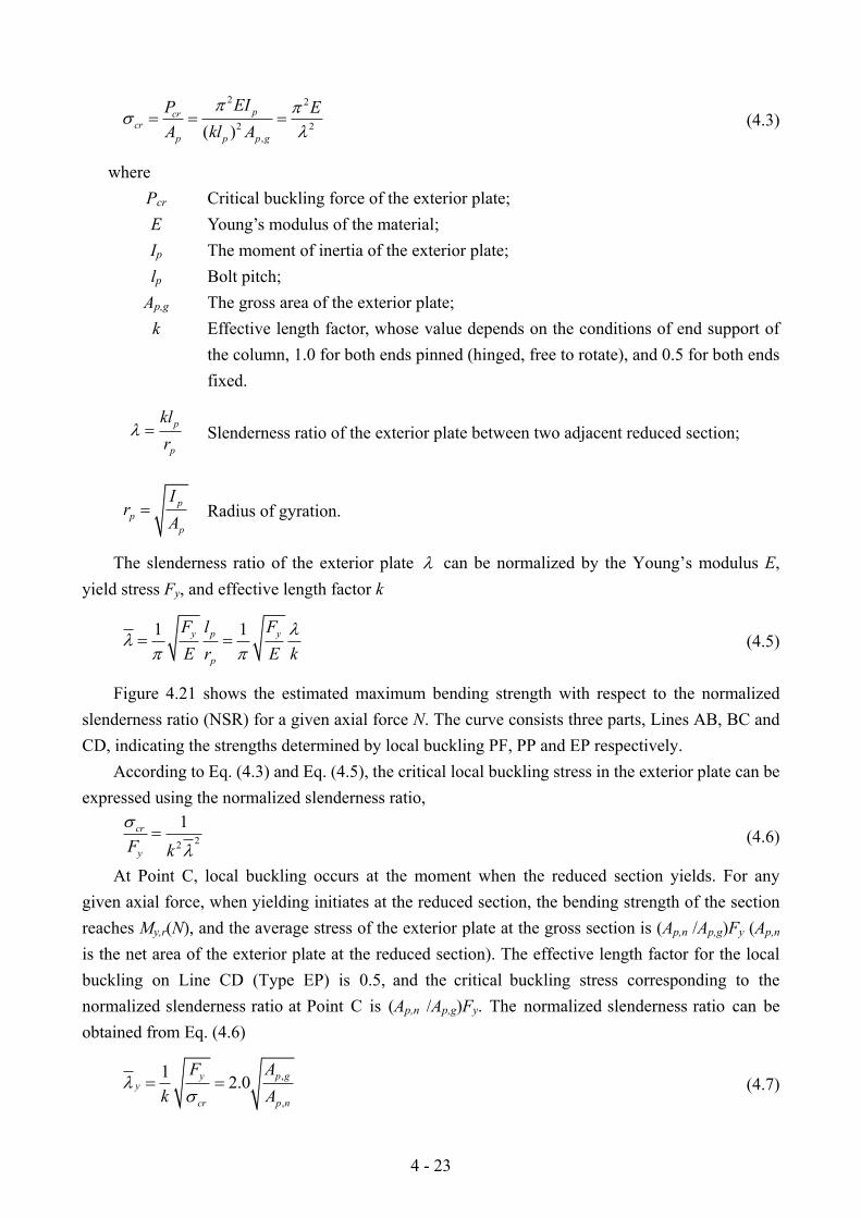
4 - 23

2 2

2 2

,( )

pcrcr

p p p g

EIP E

A kl A

(4.3)

where

Pcr Critical buckling force of the exterior plate;

E Young’s modulus of the material;

Ip The moment of inertia of the exterior plate;

lp Bolt pitch;

Ap,g The gross area of the exterior plate;

k Effective length factor, whose value depends on the conditions of end support of

the column, 1.0 for both ends pinned (hinged, free to rotate), and 0.5 for both ends

fixed.

p

p

kl

r

Slenderness ratio of the exterior plate between two adjacent reduced section;

p

p

p

Ir

A

Radius of gyration.

The slenderness ratio of the exterior plate can be normalized by the Young’s modulus E,

yield stress Fy, and effective length factor k

1 1y p y

p

F l F

E r E k

(4.5)

Figure 4.21 shows the estimated maximum bending strength with respect to the normalized

slenderness ratio (NSR) for a given axial force N. The curve consists three parts, Lines AB, BC and

CD, indicating the strengths determined by local buckling PF, PP and EP respectively.

According to Eq. (4.3) and Eq. (4.5), the critical local buckling stress in the exterior plate can be

expressed using the normalized slenderness ratio,

22

1cr

yF k

(4.6)

At Point C, local buckling occurs at the moment when the reduced section yields. For any

given axial force, when yielding initiates at the reduced section, the bending strength of the section

reaches My,r(N), and the average stress of the exterior plate at the gross section is (Ap,n /Ap,g)Fy (Ap,n

is the net area of the exterior plate at the reduced section). The effective length factor for the local

buckling on Line CD (Type EP) is 0.5, and the critical buckling stress corresponding to the

normalized slenderness ratio at Point C is (Ap,n /Ap,g)Fy. The normalized slenderness ratio can be

obtained from Eq. (4.6)

,

,

12.0

y p gy

cr p n

F A

k A

(4.7)

4 - 24

The strength on Line CD can be calculated by the elastic critical local buckling stress using

Eq.(4.6).

At Point B, local buckling occurs when the longitudinal stress at the reduced section of the

exterior plate reaches Fu, assuming that the post-yield stiffness at the stress of Fu is reduced to zero.

The corresponding critical local buckling stress at the gross section of the plate is (Ap,n /Ap,g)Fu. The

effective length factor for the local buckling on Line BC (Type PP) is 1.0, and the critical

normalized slenderness ratio at Point B can be obtained from Eq. (4.6)

,

,

1.0p g y

p

p n u

A F

A F (4.8)

For steel material, the strain at Fu is usually more than 10 times of the strain at Fy, the reduced

column section can be regarded to achieve a moment larger than Mp,r. Conservatively, Mp,r is used

as the estimated strength at Point B.

As normalized slenderness ratio decreases from p , the column may be able to achieve an even

higher strength. Although the test results indicated that the maximum strength could go beyond the

rupture moment, its estimation is conservatively limited to Mp,r.

Therefore, the estimation formula for the maximum bending moment is as follows:

For p

max ,( , ) ( )p rM N M N (4.9a)

For p y

max , ,( , ) ( ) ( )y p

p r y ry p y p

M N M N M N

(4.9b)

For y

2

max ,2( , ) ( )

y

y rM N M N

(4.9c)

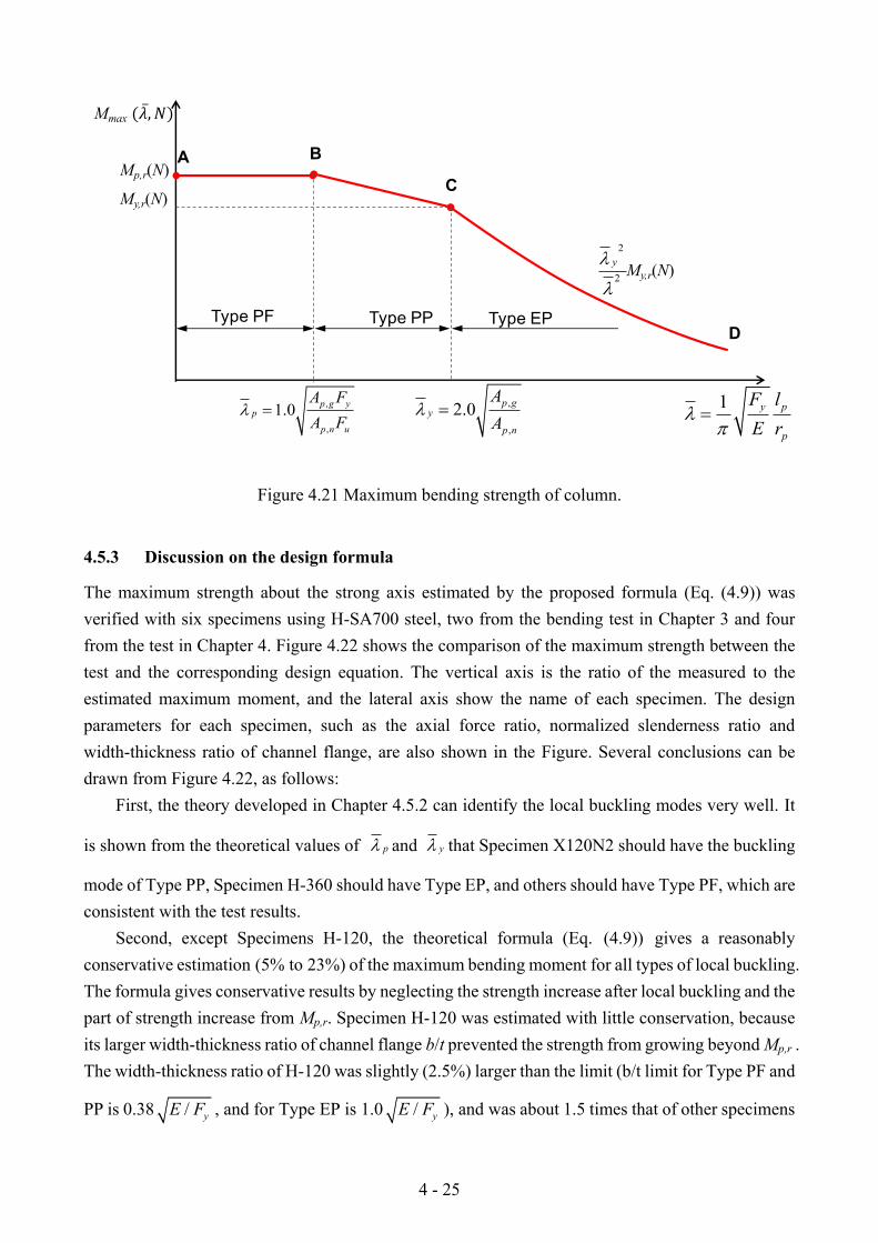
4 - 25

Mmax

Mp,r(N)

My,r(N)

A

C

2

2

y

My,r(N)

Type EPType PPType PF

1 y p

p

F l

E r

,

,

1.0p g y

p

p n u

A F

A F

,

,

2.0p g

y

p n

A

A

B

D

Figure 4.21 Maximum bending strength of column.

4.5.3 Discussion on the design formula

The maximum strength about the strong axis estimated by the proposed formula (Eq. (4.9)) was

verified with six specimens using H-SA700 steel, two from the bending test in Chapter 3 and four

from the test in Chapter 4. Figure 4.22 shows the comparison of the maximum strength between the

test and the corresponding design equation. The vertical axis is the ratio of the measured to the

estimated maximum moment, and the lateral axis show the name of each specimen. The design

parameters for each specimen, such as the axial force ratio, normalized slenderness ratio and

width-thickness ratio of channel flange, are also shown in the Figure. Several conclusions can be

drawn from Figure 4.22, as follows:

First, the theory developed in Chapter 4.5.2 can identify the local buckling modes very well. It

is shown from the theoretical values of p and y that Specimen X120N2 should have the buckling

mode of Type PP, Specimen H-360 should have Type EP, and others should have Type PF, which are

consistent with the test results.

Second, except Specimens H-120, the theoretical formula (Eq. (4.9)) gives a reasonably

conservative estimation (5% to 23%) of the maximum bending moment for all types of local buckling.

The formula gives conservative results by neglecting the strength increase after local buckling and the

part of strength increase from Mp,r. Specimen H-120 was estimated with little conservation, because

its larger width-thickness ratio of channel flange b/t prevented the strength from growing beyond Mp,r .

The width-thickness ratio of H-120 was slightly (2.5%) larger than the limit (b/t limit for Type PF and

PP is 0.38 / yE F , and for Type EP is 1.0 / yE F ), and was about 1.5 times that of other specimens

4 - 26

with the same local buckling mode.

Third, the ratio of the measured to estimated strength become larger as the axial force ratio

increases, which is independent of local buckling modes.

Figure 4.23 shows how the axial force ratio affects the estimation. The maximum bending

moments were obtained from the finite element analysis in Figure 4.16. The results denoted as FEM

(pitch=60) are from the column that sustained local buckling of Type PF under any axial force ratio,

while those denoted as FEM (pitch=120) are from the column that sustained local buckling of Type

PP. Although FEM (pitch=60) and FEM (pitch=120) sustained different local buckling modes, their

ratios of the strength from FEM to the estimated strength are almost the same under the same axial

force ratio, and increase as the axial force become larger. Therefore, Eq. (4.9) may become too

conservative for large axial force ratios. Specifically, the Eq. (4.9) presents reasonably conservative

estimation on the strength (5% to 23% smaller) when the axial force ratio is no more than 0.4, and is

too conservative for the axial force ratio larger than 0.4 (e.g., about 31% of underestimation at axial

force ratio of 0.6).

Mmax (Est.)

0

0.2

0.4

0.6

0.8

1

1.2

1.4

0.70 0.700.70 1.400.91 2.42

B/t 0.26y

E

F0.39

y

E

F0.26

y

E

F0.39

y

E

F0.26

y

E

F0.26

y

E

F

N/N0 0.0 0.40.2 0.00.0 0.2

Type PF Type PP Type EP

Specimen X60N0 X60N2 X60N4 H-120 H-360X120N2

Mmax (Test)

p =1.06 y =2.19Note:

Figure 4.22 Comparison between test results and the estimation for different local buckling modes.

4 - 27

0

0.2

0.4

0.6

0.8

1

1.2

1.4

1.6

0 0.2 0.4 0.6 0.8

Axial force ratio N/N0

Mmax (Est.)

Mmax (FEM)

FEM (pitch=60) =0.70

=1.40FEM (pitch=120)

p =1.06 y =2.19Note:

Figure 4.23 Effect of axial force ratio on the estimation of the maximum strength.

4.6 Summary

Behavior of the column subjected to the combined bending and axial force was investigated by tests

of five specimens, and finite element analysis. The basic conclusions are as follows:

(1) The column exhibited a very large yield rotation exceeding 0.018 rad under an axial force

ratio of 0.2. The measure elastic bending stiffness was within 7% difference from the

estimated value based on the assumption that plane sections remain plane, and using the

gross area of the section;

(2) The column strength was mainly limited by the net area of the reduced section. The yield

strength was inversely proportional to the axial force, and can be estimated very well by the

proposed formula. The maximum flexural strength of the specimens exceeded the rupture

moment of the reduced section.

(3) Finite element analysis was carried out for supplementing the experimental findings. The

finite element model was verified in its effectiveness with all specimens, and showed good

performance on tracing the stiffness, strength and failure mode for the columns with various

axial force ratios, bolt pitches and loading directions.

(4) The axial force ratio versus maximum bending moment relationships for the specimens with

different bolt pitches were obtained through the parametric study using the proposed finite

element model. The relationship can be approximately described with two straight lines, one

for small axial force ratios and the other for large axial force ratios.

(5) Although the boundary condition at the bottom of the column affected the maximum

bending strength and local strain distribution, the influence on the strength and its

4 - 28

deterioration under cyclic loading was limited, and the maximum difference on the strength

was 4.5% with respect to the baseline specimen.

(6) A design formula to estimate the bending strength of the column under an axial force was

established and verified by the tests and finite element analysis. The formula gave a

reasonably conservative estimation (by 5%~23%) for columns with an axial force ratio not

larger than 0.4. As the axial force ratio increases, the estimation becomes more conservative.

REFERENCES

[1] Zhou F, Matsumiya T, Kurata M, Suita K (2003). Strength and mechanical behavior of bolted

column base connection. Journal of Constructional Steel, JSSC, Vol.11, pp.583-590, Nov. 2003.

[2] Suita K, Inoue K, Takeuchi I, Uno N (2003). Mechanical behavior of bolted beam-to-column

connections with buckling-restrained knee brace dampers. Journal of Structural and

Construction Engineering, AIJ, No.571, 153-160, Sep. 2003.

[3] American Institute of Steel Construction (AISC) (2003). Extended End-Plate Moment

Connections (Seismic and Wind Applications), Second Edition, 2003.

[4] Korol RM, Ghobarah A, Osman A (1990). Extended End-plate connections under cyclic loading:

behavior and design. Journal of Constructional Steel Research, 16(1990): 253-280.

[5] MSC. Software Corporation. MSC (2008). Marc User's Manual (Marc 2008 R1, Volume A,

Theory and user information). Santa Ana, CA 92707, USA. MSC.Software Corporation.

[6] MSC. Software Corporation. MSC (2008). Marc User's Manual (Marc 2008 R1, Volume B,

Element Library). Santa Ana, CA 92707, USA. MSC.Software Corporation.

[7] Sumner EA (2003). Unified design of extended end-plate. Doctoral Dissertation, Virginia

Polytechnic Institute and State University, Blacksburg, Virginia.

[8] Shi G, Shi Y, Wang Y, Bradford MA (2008). Numerical simulation of steel pretensioned bolted

end-plate connections of different types and details. Engineering Structures, 30:2677-2686.

[9] American Iron and Steel Institute (2007). North American Specification for the Design of

Cold-Formed Steel Structural Members (2007 Edition).

[10] Architectural Institute of Japan (AIJ) (2009). Recommendations for Stability Design of Steel

Structures.

[11] American Institute of Steel Construction (AISC) (2010). Specification for Structural Steel

Buildings, June 22, 2010.

[12] Rasmussen K.J.R., Hancock G.J. (1992). Plate slenderness limits for high strength steel sections.

J. Construct. Steel Research, 23:73-96.

5 - 1

CHAPTER 5

Behavior of Unstiffened Local Connections of Column

Subjected to Concentrated Forces

5.1 Introduction 5.1.1 Background and objective Independent of the column behavior investigated in Chapters 3 and 4, the column behavior studied in this chapter focuses on the column-side limit states due to bolted local connection. Local connections, which usually exert concentrated perpendicular tensile or compressive force to the column, exist extensively in steel structures. In the prototype structural system, bolted connections are adopted exclusively for all connections that join structural members. Figure 5.1 shows illustration examples for local connections in two types of typical bolted moment beam-to-column connections, extended end-plate connection and spilt tee connection [1~3]. The bending moment of the beam is transferred to the column mainly by the tension of one beam flange and the compression of the other beam flange. The tensile or compressive force from the beam flange acts on the column flange and may cause local failure in the column web or flange. The AISC Specification for Structural Steel Buildings (2010) [3] list six different limit states for the flanges and web of column with concentrated forces:

1. Flange local bending, only applied to tensile forces; 2. Web local yielding, applied to both tensile and compressive forces; 3. Web crippling, only applied to compressive force; 4. Web sidesway buckling, only applied to compressive force; 5. Web compression buckling, only applied to compressive force; 6. Web panel zone shear, only applied to compressive force. The limit states shown in the specification is applied mainly to welded moment connections

rather than bolted connections. Carter [4] gave a design method to limit state 1 for the end-plate connections. However, the corresponding design formulas in these codes are applicable only to the

5 - 2

columns of rolled sections or welded built-up sections, rather than the proposed bolted built-up columns using cold formed channels (see Chapter 2). Although American Specification for the Design of Cold-Formed Steel Structural Members [5] gives formula to estimate web crippling strength of cold-formed channels, the empirical design formula might not be applicable for channels using ultra-high-strength steel. Behavior of the proposed column under concentrated tensile or compressive force may be distinctly different with that of the rolled or welded column for three reasons:

(1) The column flange consists of two layers of plates (the exterior plate and the channel flange), which are connected continuously by bolts and interacted with each other;

(2) The bent portion of the inner channels gives flexible and complex boundaries for the column web and flanges, so the transferring mechanism of force from the flange to the web may differ from that expected in the rolled or welded columns;

(3) The connection behavior may be different since the column uses the new steel (H-SA700) with very high strength, and rupture may also occur as the rupture elongation of the steel is about 12%.

Because of these significant differences of the proposed column, several targets were addressed in this chapter, as shown below:

(1) To examine the failure mode and force transferring mechanism of the built-up column subjected to concentrated force;

(2) To evaluate the strength of connections joined to the unstiffened column and verify the design equation.

(3) To examine whether stiffeners are needed and how to reinforce the connection and provide design information for preparation of the test on the bolted beam-to-column connections.

M

Local connection under tensile force

Local connection under compressive force

M

(a) (b) Figure 5.1 Local connections in bolted beam to column connections: (a) extended end-plate

connection; (b) split tee connection.

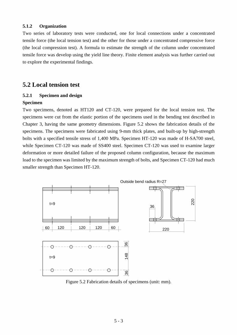
5 - 3

5.1.2 Organization Two series of laboratory tests were conducted, one for local connections under a concentrated tensile force (the local tension test) and the other for those under a concentrated compressive force (the local compression test). A formula to estimate the strength of the column under concentrated tensile force was develop using the yield line theory. Finite element analysis was further carried out to explore the experimental findings.

5.2 Local tension test 5.2.1 Specimen and design Specimen Two specimens, denoted as HT120 and CT-120, were prepared for the local tension test. The specimens were cut from the elastic portion of the specimens used in the bending test described in Chapter 3, having the same geometry dimensions. Figure 5.2 shows the fabrication details of the specimens. The specimens were fabricated using 9-mm thick plates, and built-up by high-strength bolts with a specified tensile stress of 1,400 MPa. Specimen HT-120 was made of H-SA700 steel, while Specimen CT-120 was made of SS400 steel. Specimen CT-120 was used to examine larger deformation or more detailed failure of the proposed column configuration, because the maximum load to the specimen was limited by the maximum strength of bolts, and Specimen CT-120 had much smaller strength than Specimen HT-120.

t=9

Outside bend radius R=27

t=9

12060 120 120 60 220

220

36

148

3636

Figure 5.2 Fabrication details of specimens (unit: mm).

5 - 4

Table 5.1 Material properties and strength of specimens

Specimen Material Estimated strength

(kN) Steel t (mm)

Fy (MPa)

Fu (MPa)

Elongation (%)

HT-120 H-SA700 9.03 768 814 12 533 CT-120 SS400 8.66 358 458 27 229

Design formula

The yield line theory [6~8] was used to develop the formula to estimate the strength of local connection of the column under the perpendicular tensile force. The adopted yield pattern on a channel flange is shown in Figure 5.3. The details of the theoretical study on developing the design formula are shown in Chapter 7. The strength of the column corresponding to this yield pattern is

04(16 )t

p mR Mp n p n

= +− −

(5.1)

where

/420 yc FtM = The plastic bending moment for a unit length of plate;

tc The thickness of the channel flange; Fy The yield stress of the channel.

p, n, m Geometry parameters related with the channel width and locations of bolt holes (see Figure 5.3).

The value of s can be determined by

)( npps −= (5.2)

The strengths of the specimens calculated by Eq. (5.1) are shown in Table 5.1.

4

1

8 3

2

57

6

np

s

m

s

x

0.5Tf

Exterior plateEnd plate

Channel webTf

Tf

Tf

Channel webEnd plate

1 1

Section1-1

Figure 5.3 Yield pattern adopted for strength estimation.

5 - 5

5.2.2 Test setup Figure 5.4 shows the setup for the local tension test. The specimen was fixed into the 1,000 kN loading system by two Tee connectors. Each connector had one end clamped by the loading system and the other end fixed to the column flange by bolts. The Tee connector was used to represent the boundary condition provided by the bolted beam-to-column connections (see Figure 5.1). The detailed dimensions of the Tee connectors are shown in Figure 5.5. The maximum tensile force exerted to the column flange was 600 kN, which was limited by the total tensile strength of four high-strength bolts.

Specimen

Bolts

Tensile forceTee connector

(a) (b)

Figure 5.4 Test setup of local tension test: (a) testing machine and specimen; (b) drawings of the specimens and setup.

Sym.

25

180

77.5 77.5

104

12

104

220

148

120

φ18

Sym.

25

18080

12

220

100

Figure 5.5 Details of the stiffened Tee (unit: mm).

5 - 6

5.2.3 Test results and analysis Figure 5.6 shows the residual deformation of each specimen after the test, and Figure 5.7 shows the load versus flange perpendicular displacement relationships for the two specimens. The perpendicular displacement in the figure was defined as half of the displacement measured from the end plate of the bottom Tee connector to that of the top Tee connector. Because the specimen was symmetric between the bottom and the top, the displacement in the figure was the average deformation of the two column flanges. The strain gauges that were used to monitor the yielding state in the channel were shown in Figure 5.6. Strain gauges No.15-20 were on the channel flange, and No.10~14 were on the channel web. The locations of No.10 and 14 were located at the two ends of Yield line 8 (s=55 mm, see Figure 5.3). The triangle marker indicates the location when the yielding initiated (at the gauge of No. 18 on the flange due to compression), and the circle marker indicates the location of the curve when yielding spread to a larger area and formed the yield pattern (at the gauges of No. 18, 15, 17, 11, 13, 12, 10, 14, 19). The estimated strength formed for each specimen is also shown in the figure.

In Specimen HT-120, yielding was first found at the gauge location of No.18 under the load of 341 kN (see the triangle marker), and then at No. 15, 17, 11, 13, 12, 10, 14, 19 under the load of 558 kN (see the solid round marker). The strains at No. 20 and 16 were much smaller than others, and did not go beyond the yield strain through the entire loading process. The yield pattern was formed when the load reached 558 kN, which was close to the estimated strength. The strength kept increasing and the stiffness gradually decreased as the loading continued further from the initiation of yielding, and the maximum strength of Specimen HT-120 was not obtained in the test. The residual deformation (about 3 mm) was observed, although the load went over the estimated strength slightly.

Specimen CT-120 yielded under the load of 138 kN, and formed the yield pattern under the load of 254 kN. Although Specimen CT-120 had a much smaller strength than Specimen HT-120, it presented a similar failure mode and yield pattern, and the maximum strength was not achieved up to the end of loading. The strength grew to about three times the estimated strength at the end of loading, and the stiffness became stable after reaching the estimated strength. When it was unloaded, the deformation was not recovered (see Figure 5.6(b)).

It is shown from Figure 5.7 that the design formula Eq. (5.1) presented a stable estimation on the load when the yield pattern formed. The estimation was slightly conservative for estimating the strength when the yield pattern was detected by strain gauges (4.5% smaller for Specimen H-120, and 9.8% smaller for Specimen C-N120). Although the column exhibited significant strength increase after yielding, the plastic deformation grew very fast, which should not occur, however, for the column that remains elastic in a rare earthquake.

5 - 7

(a) (b)

Figure 5.6 Residual deformation: (a) HT-120; (b) CT-120.

0

100

200

300

400

500

600

700

0 5 10 15 20 25

Test_HT120 Test_CT120

Load

(kN

)

HT-120 (Estimated strength)15 16 17

1819 20

4510 11 12 13 14

First yielding (Gauge 18)

Formation of the yield pattern (Gauges 18, 15, 17, 11, 12, 13,10,14,19)

CT-120 (Estimated strength)

Flange perpendicular displacement (mm)

Figure 5.7 Load versus flange perpendicular displacement relationship

5.2.4 Finite element analysis Modeling Finite element analysis was conducted to simulate the local tension test mainly for two reasons. First, the finite element analysis provided visualized contour to see the detailed yield pattern in terms of the plastic strain, which helped obtain better understanding on the test results. Second, the practical maximum load exerted on the specimen was limited by the bolt strength, and the finite element analysis enabled a larger load by increasing the strength of bolts. The model was constructed in the engineering simulation software ABAQUS 6.10. Figure 5.8 shows the finite element model used for the analysis. Only one eighth of the specimen was modeled, as shown in Figure 5.8(a), and the boundary conditions for mirror symmetry were set on all three reference planes of the one-eighth model. Figure 5.8(b) shows a picture of the model by mirror displays referring to XY, XZ and YZ planes, and the picture exhibited a view of specimen that is exactly the same as the specimen shown in the photo (see Figure 5.4).

5 - 8

Bolts were modeled explicitly (see Figure 5.8(a)) for the connection to a Tee connector, and the pretension forces were simulated by setting initial stress in the bolts. Contact was set at the interfaces between all components, such as bolt, Tee connector, plates and channels. Interaction between the mating surfaces was defined by full force transfer in the direction normal to the surface and a friction coefficient of 0.45 (the surface was clean and rusted) in the direction perpendicular to the surface. The same eight-node reduced-integration solid elements, which were also used for the model in Chapters 3 and 4, were used for the model. The material properties in Table 5.1 were used for the nonlinear material model, and tri-linear model [8, 9] in Figure 4.9 was used for the bolt material (for F14T bolts, the specified minimum yield stress is 1,260 MPa and the specified minimum tensile stress is 1,400 MPa).

(a) (b) Figure 5.8 Finite element model: (a) one-eighth model; (c) view of the model after mirror display.

Verification

Both of the specimens were simulated by the proposed one-eighth model in Figure 5.8, and the comparisons of results between the finite element analysis and test in terms of the load versus flange perpendicular displacement relationship are shown in Figure 5.9. The model represented the load versus flange perpendicular displacement relationship very well for both specimens, and for either loading or unloading. Figure 5.10 shows the residual deformations of Specimen CT-120 by the picture from finite element analysis (see Figure 5.10(a)) and the photo from the test (see Figure 5.10(b)). The model achieved a very similar shape mode to the test for residual deformations. Hence, the model was verified to reasonably duplicate the strength and residual deformation of the specimens.

5 - 9


Load

(kN

)

0

100

200

300

400

500

600

700

0 5 10 15 20 25

Test_HT120 FEM_HT120

Test_CT120 FEM_CT120

Figure 5.9 Comparison of load versus flange perpendicular displacement relationship

Figure 5.10 Comparison of residual deformation (CT-120): (a) a picture from the finite element

analysis; (b) a photo from the test.

Analysis Although the maximum load in the test was limited by the strength of high-strength bolts, larger

load was still possible in the finite element analysis by using virtual stronger bolts (not exist practically). The stronger bolts were achieved by changing the tri-linear material model in Figure 4.9 into a bilinear material model, which only used the first and second lines. The completely elastic bolts model was not used for maintaining the consistency of the loading conditions between the simulation results and test results up to the tested maximum load. The virtual bolts had the same yield strength as those used in the tests, but had an infinite large maximum strength. Much larger load, about two times of the estimated strength, was applied to HT120. An even larger load failed to be applied due to the convergence problems. Figure 5.11 shows the load versus flange perpendicular displacement relationship from the analysis using virtual stronger bolts (denoted by FEM_HT120(SBolt)).

Similar to the behavior of Specimen CT-120, the stiffness of Specimen HT-120 became stable after the yield pattern initiated (see Point A, close to the estimated strength), the strength kept increasing to the end of loading (see Point B). The yield patterns for Points A and B are shown in

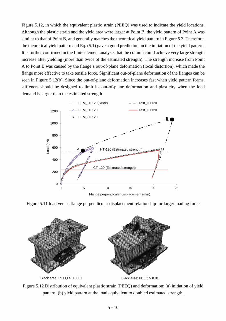
5 - 10

Figure 5.12, in which the equivalent plastic strain (PEEQ) was used to indicate the yield locations. Although the plastic strain and the yield area were larger at Point B, the yield pattern of Point A was similar to that of Point B, and generally matches the theoretical yield pattern in Figure 5.3. Therefore, the theoretical yield pattern and Eq. (5.1) gave a good prediction on the initiation of the yield pattern. It is further confirmed in the finite element analysis that the column could achieve very large strength increase after yielding (more than twice of the estimated strength). The strength increase from Point A to Point B was caused by the flange’s out-of-plane deformation (local distortion), which made the flange more effective to take tensile force. Significant out-of-plane deformation of the flanges can be seen in Figure 5.12(b). Since the out-of-plane deformation increases fast when yield pattern forms, stiffeners should be designed to limit its out-of-plane deformation and plasticity when the load demand is larger than the estimated strength.

0

200

400

600

800

1000

1200

0 5 10 15 20 25

FEM_HT120(SBolt) Test_HT120

FEM_HT120 Test_CT120

FEM_CT120

Load

(kN

)

HT-120 (Estimated strength)

CT-120 (Estimated strength)


A

B

Figure 5.11 load versus flange perpendicular displacement relationship for larger loading force

Black area: PEEQ > 0.0001 Black area: PEEQ > 0.01 Figure 5.12 Distribution of equivalent plastic strain (PEEQ) and deformation: (a) initiation of yield

pattern; (b) yield pattern at the load equivalent to doubled estimated strength.

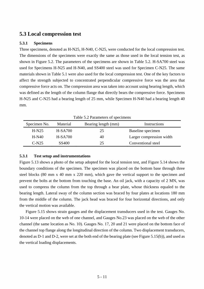
5 - 11

5.3 Local compression test 5.3.1 Specimens Three specimens, denoted as H-N25, H-N40, C-N25, were conducted for the local compression test. The dimensions of the specimens were exactly the same as those used in the local tension test, as shown in Figure 5.2. The parameters of the specimens are shown in Table 5.2. H-SA700 steel was used for Specimens H-N25 and H-N40, and SS400 steel was used for Specimen C-N25. The same materials shown in Table 5.1 were also used for the local compression test. One of the key factors to affect the strength subjected to concentrated perpendicular compressive force was the area that compressive force acts on. The compression area was taken into account using bearing length, which was defined as the length of the column flange that directly bears the compressive force. Specimens H-N25 and C-N25 had a bearing length of 25 mm, while Specimen H-N40 had a bearing length 40 mm.

Table 5.2 Parameters of specimens Specimen No. Material Bearing length (mm) Instructions

H-N25 H-SA700 25 Baseline specimen H-N40 H-SA700 40 Larger compression width C-N25 SS400 25 Conventional steel

5.3.1 Test setup and instrumentations Figure 5.13 shows a photo of the setup adopted for the local tension test, and Figure 5.14 shows the boundary conditions of the specimen. The specimen was placed on the bottom base through three steel blocks (80 mm x 40 mm x 220 mm), which gave the vertical support to the specimen and prevent the bolts at the bottom from touching the base. An oil jack, with a capacity of 2 MN, was used to compress the column from the top through a bear plate, whose thickness equaled to the bearing length. Lateral sway of the column section was braced by four plates at locations 180 mm from the middle of the column. The jack head was braced for four horizontal directions, and only the vertical motion was available.

Figure 5.15 shows strain gauges and the displacement transducers used in the test. Gauges No. 10-14 were placed on the web of one channel, and Gauges No.23 was placed on the web of the other channel (the same location as No. 10). Gauges No. 17, 20 and 21 were placed on the bottom face of the channel top flange along the longitudinal direction of the column. Two displacement transducers, denoted as D-1 and D-2, were set at the both end of the bearing plate (see Figure 5.15(b)), and used as the vertical loading displacements.

5 - 12

(a) (b) Figure 5.13 Test setup for local compression test (test photos): (a) global view; (b) local view.

Plate to prevent lateral sway of section

Bearing plate

Blocks to prevent the bolts touching the base

Load Load

Figure 5.14 Boundary conditions of the specimen.

2730

30

30 30

10

13

14

11 1217 21 20

10

13

14

23

20

D-1 D-2

A

A Section A-A

(a) (b) Figure 5.15 Strain gauges and displacement transducers (unit: mm).

5 - 13

5.3.3 Test results and analysis Figure 5.16 shows the load-vertical displacement (positive value is the pushing direction of the jack) relationship for each specimen. The loading stopped if the load reached 1.5 MN (for the safety of the loading system) or the specimen exhibited very severe deformation.

All specimens presented a similar failure mode, and taking the baseline specimen H-N25 as an example, the failure mode was as follows: First, the channels yielded at the load of 310 kN, which was detected by the strain gauges shown in Figure 5.15. Second, as plasticity grew, local distortion occurred in both the column top flange and the upper portion of the webs, both located at the middle of the column (indicated by Point A on the curve, and the deformation was shown in Figure 5.17(a)). Third, as the local distortion was enlarged, the load increased little, but the vertical displacement grew significantly (from 12 mm to 35 mm), and the two webs of the channel pair touched each other at the load of 974kN (indicated by Point B, and the deformation is shown in Figure 5.17(b) ). Finally, due to the touching of the two webs, the stiffness increased significantly, and the load grew to about 1.5 MN. The strength was very large, but yielding initiated very early, which was about one fifth of the maximum load.

0

400

800

1200

1600

0 10 20 30 40 50

H-N25 H-N40 C-N25

AB

Vertical displacement (mm)

Load

(kN

)

Yield at 303kN (H-N40)Yield at 310kN (H-N25)

Yield at 106kN (C-N25)

C

Figure 5.16 Load-vertical displacement relationships for specimens It seems against the conventional design concept that Specimen H-N40 had a larger bearing

length than Specimen H-N25, but exhibited a slightly smaller yielding strength. In fact, these two specimens yielded at different locations. Specimen H-N25 yielded first at the channel flange (at the gauge of No.20), while Specimen H-N40 at the webs (at the gauges of No. 10 and 23). A smaller bearing length induced more severe concentration of force in the flange, while a larger bearing length tended to induce local bending in the webs that was close to the top bend portion of the channels. Because the bend portion did not provide a stiff and clear boundary between the channel flange and web, the strength due to concentrated force may not increase effectively by simply enlarging the bearing length.

Specimen C-N25 was loaded to a larger displacement, because of its smaller strength. More

5 - 14

failure details were observed through this specimen. After the webs touched each other, more area of the webs began to touch from the top to the bottom. When the bottom portion of the web joined the touching (indicated by Point C in Figure 5.16 and its deformation shown in Figure 5.17(c)), the stiffness increased again and the load began to grow to a larger level (larger than 800 kN).

Although exhibited very high strength under a perpendicular concentrated compressive force, the column yielded very early, and had large residual deformation after unloading (e.g, 35 mm residual displacement was observed in Specimen H-N25 after unloading from the vertical displacement of 40 mm). Stiffeners are needed to limit the plasticity and local deformation of the column under local compressive force. It is shown from the failure modes of all specimens that the effective to increase the stiffness and strength of the web is to prevent the web from local bending.

(a) (b) (c)

Figure 5.17 Deformation of Specimens: (a) slight local deformation (H-N25); (b) touching of the webs (H-N25); (c) completely touching of the webs (C-N25).

5.3.4 Finite element analysis Modeling Only half of the specimen was modeled, because the specimen deformed good symmetry along the longitudinal direction of the column, as shown in Figure 5.18. The contact parameters and material properties were kept the same as those in the model for local tension test. Since the bolts did not vary in tensile force during the loading, the bolt force was simulated by an equivalent pressure force distributed to an area (the same as the area of the washer) around the bolt hole. Verification

All specimens were used to verify the performance of the finite element model. Figure 5.19 shows the load-vertical displacement relationships of all specimens from both the test and finite element analysis. The loading in the finite element analysis did not stop unless the model failed to converge, and all simulated cases were able to go beyond the critical point at which two webs touched each other. The load-vertical displacement relationship from the proposed model generally matched that from test, and particularly, the model well traced very reasonably the displacement at which the two webs touched each other (like Point B in Figure 5.16).

5 - 15

(a) (b)

Figure 5.18 Model: (a) half model; (b) the global view of the specimen through mirror display.

0

300

600

900

1200

1500

1800

0 10 20 30 40 50 60

Test (H-N25) Test (C-N25) Test (H-N40)

FEM (H-N25) FEM (C-N25) FEM (H-N40)


Load

(kN

)

D

Figure 5.19 Comparison of load-vertical displacement relationship.

The simulated deformation (Specimen H-N25) for the moment when the two webs touched, as

shown in Figure 5.20(a), had good agreement with the observed deformation in the test, as shown in Figure 5.17(a). The finite element analysis for Specimen H-N25 did not come across convergence problems until it reached the vertical displacement of 57 mm. The two webs of Specimen H-N25 completely touched each other at 50 mm (Point D in Figure 5.19), as shown in Figure 5.20(b), and similar phenomenon was observed for Specimen C-N25, as shown Figure 5.17(c). The model duplicated reasonably the deformation details at the critical points.

5 - 16

0.0100

0.0075

0.0050

0.0025

0.0000

(a)

(b)

PEEQ

Figure 5.20 Simulated deformation of Specimen H-N25: (a) touching of the webs; (b) completely

touching of the webs.

Analysis Four cases, H-N25, H-N40, H-N80 and H-N25SW, were compared based on the proposed finite

element model. Cases, H-N25 and H-N40, were exactly the same as Specimens H-N25 and H-N40. Case H-N80 was designed for examining the effect of bearing length, and had the same column as H-N25 but used a larger bearing length of 80 mm. Case H-N25SW had stiffened webs based on Case H-N25, and was used to seek possible way of stiffening the column. The stiffened zone is shown in Figure 5.21. The stiffening effect was simply simulated by making all the nodes of this zone in a rigid plane, which means no out-of-plane deformation was allowed in the stiffened web zone.

Figure 5.21 shows the load-vertical displacement relationships for all the cases. It is found from the comparison between Cases H-N25, H-N40 and H-N80 that the strength of the column was increased by simply enlarging the bearing length, although the displacement that caused touching between two webs decreased as the bearing length increased. The strength of the column was mainly affected by similar local distortion at the top ends of the webs. It is shown from the comparison between Cases H-N25 and H-N25SW that the vertical deformation after yielding was significantly reduced by preventing the local distortion in the webs. Specifically, the ratio of the vertical displacement between Case H-N25SW and Case H-N25 was 1:2 under the load of 800kN (web local distortion was observed in Case H-N25), and 1:3 under the load of 1080kN (touching occurred between the webs in Case H-N25). Therefore, stiffeners that can increase the out-of-plane stiffness of the web, may be effective to reinforce the column subjected to concentrated compressive force.

The proposed model may be used for further parameter analysis to investigate the column behavior under concentrated compressive forces.

5 - 17

180 mm

0

400

800

1200

1600

2000

0 10 20 30 40 50 60

FEM (H-N80)

FEM (H-N25,Stiffened Web)

FEM (H-N25)

FEM (H-N40)


Load

(kN

)

Stiffened zone on webFEM (H-N25SW, Stiffened Web)

Figure 5.21 Load-vertical displacement relationships for all the cases.

5.4 Summary Behavior of unstiffened bolted built-up columns subjected to concentrated perpendicular force, tensile force or compressive force, was investigated by experiments and finite element analysis. The major findings from the experiment and finite element analysis are as follows:

For unstiffened columns subjected to concentrated tensile force, (1) The column exhibited significant strength increase after the yield pattern formed. (2) Since the out-of-plane deformation increased fast when yield pattern formed, stiffeners

should be arranged to limit its out-of-plane deformation and plasticity when the load demand is larger than the estimated strength.

(3) The proposed formula based on the yield line theory was slightly conservative (by 5%~10%) for the strength at the formation of yield pattern.

For unstiffened column subjected to concentrated compressive force, (1) Although the column yielded under a small load, the strength kept increasing after yielding,

and the maximum strength observed in the loading was five times the yield strength. (2) The strength was not affected significantly by simply enlarging the bearing length (by 25

mm to 80 mm). (3) The vertical displacement of the column after yielding was cut by half through stiffening the

webs from local distortion. (4) Stiffeners that can increase the out-of-plane stiffness of the web, are effective to reinforce

the column subjected to concentrated compressive force.

5 - 18

REFERENCES [1] Architectural Institute of Japan (AIJ) (2012). Recommendation for Design of Connections in

Steel Structures. [2] American Institute of Steel Construction (AISC) (2003). Extended End-Plate Moment

Connections (Seismic and Wind Applications), Second Edition, 2003. [3] American Institute of Steel Construction (AISC) (2010). Specification for Structural Steel

Buildings, June 22, 2010. [4] Carter, CJ (1999). Stiffening of Wide-Flange Columns at Moment Connections: Wind and

Seismic Applications, Design Guide 13, AISC, Chicago, IL. [5] American Iron and Steel Institute (2007). North American Specification for the Design of

Cold-Formed Steel Structural Members (2007 Edition). [6] Johansen KW (1972). Yield-line Formulae for Slabs, Cement and Concrete Association,

London, England. [7] Srouji R, Kukreti AR, Murray TM (1983). Yield-line analysis of end-plate connections with

bolt force predictions. Research Report No.FSEL/MBMA 83-05, Fears Structural Engineering Laboratory, School of Civil Engineering and Environmental Science, University of Okalahoma, Norman, Okalahoma.

[8] Sumner EA. Unified design of extended end-plate (2003). Doctoral Dissertation, Virginia Polytechnic Institute and State University, Blacksburg, Virginia.

[9] Shi G, Shi Y, Wang Y, Bradford MA (2008). Numerical simulation of steel pretensioned bolted end-plate connections of different types and details. Engineering Structures, 30:2677-2686.

6 - 1

CHAPTER 6

Behavior of Bolted Beam-to-column Connections

6.1 Introduction 6.1.1 Objectives As mentioned in Chapter 1, bolted moment connections were planned to be used about the strong axis of the proposed built-up column, and the damage in the column (including the column-side connection) should be limited to ensure the continuous use of the components after rare earthquakes. It is shown from the study of the local connections in Chapter 5 that stiffeners may be needed to avoid the early local yielding of the connections. In this chapter, the bolted moment beam-to-column connections, with or without stiffeners, were investigated for the objectives as follows:

(1) To develop a feasible scheme for connecting the column, beams, and stiffeners by using bolts but no welds;

(2) To examine the failure modes associated with low resistance of the column against tension acting perpendicular to its flanges;

(3) To develop stiffeners (continuity plates) that help overcome the weakness of the column against local tension.

6.1.2 Organization Both an experimental study and finite element analysis were conducted to examine the behavior of the beam-to-column connections. First, two types of bolted stiffeners were proposed. Second, a test program, including the specimens, test setup, loading protocol and instrumentations, was introduced. Third, test results and their analysis were presented, and the performance of the connections, with or without stiffeners, was evaluated. Last, a finite element model was proposed, and the yielding and energy dissipation of various parts of the connection were investigated.

6 - 2

6.2 Connection Patterns In the envisioned structural system, the connection to the column flange (about strong axis of the column) is a moment connection, but the connection to the column web (about weak axis of the column) may be either a moment connection or a simple shear connection. While details for all beam-to-column connection types were taken into account for the system, the moment connection to the column flange poses the biggest technical challenge. The extended end-plate connection and the split-Tee connection are two types of popular bolted moment connections [1~3], and to simplify the details of the beam-side connection, the extended end-plate connection was used for the test in this study.

T87.5x175x9x11

Flange

175

(t=6)

Flange

(t=9)

(a) (b) (c) Figure 6.1 Patterns of the beam-to-column connections: (a) no stiffener; (b) Tee stiffener; (c) angle

stiffener (unit: mm).

The connection patterns used in the test are shown in Figure 6.1. The connection without stiffeners is shown in Figure 6.1 (a). The end plates of the beam connect the column through the column flanges. In the orthogonal direction, another pair of beams connect to the column web (interior channels) through split Tees. Figure 6.1(b) shows a connection where the column is stiffened at the beam flange location using three Tees (referred to as the Tee stiffener). One Tee is the same as the one shown in Figure 6.1(a) and the other two are smaller. The stiffeners help the tension or compression force acting perpendicular to the column flange plate to be transferred more smoothly into the column. A particular concern is that the built-up column section has limited yield resistance to local tension as the flange plate can deform out-of-plane and the interior channel can unfold. The stiffeners were used to overcome this weakness by controlling the local deformation and distributing the local stress more evenly across the cross section. The nominal strength of the stiffeners is controlled by yielding of the net section of the stem of the smaller Tee and computed as 148 kN. Figure 6.1(c) shows a connection where each stiffener consists of two angle stiffeners constructed by

6 - 3

welding together three plates (referred to as the angle stiffener). This stiffener has a similar mechanism to the Tee stiffeners for transferring the perpendicular forces. As shown in Figure 6.1, the flange of the orthogonal beams connects to the column web either through multiple stiffeners or through a single Tee.

6.3 Test Program 6.3.1 Specimen To investigate the column-side connection behavior of beam-to-column connections, four specimens were prepared with different column or connection details. The specimens CN and HN had no stiffeners in the connections, as shown in Figure 6.1(a). Specimen HN was a baseline specimen, and used H-SA700 steel for its column, while Specimen CN used conventional steel (called as SS400 steel) for its column. The specimens HTS and HAS were connections stiffened by bolted stiffeners. Specimen HTS used Tee stiffeners, as shown in Figure 6.1(b), and Specimen HAS used angle stiffeners, as shown in Figure 6.1(c).

The dimensions of the columns and connections are shown in Figure 6.2. All columns had the same section. With a section of 220 mm by 220 mm, the column was made up of plates with a thickness of 9 mm, and the inner bend radius of the cold-formed channels was 18 mm, as shown in Figure 6.2(a) and (b). The flange plates and inner channels were connected by super-high-strength F14T bolts having a minimum tensile strength of 1.4 GPa. The diameter of the bolt holes was 18 mm and the diameter of the bolts was 16 mm. The bolt pitch was 240 mm throughout except that the first bolt pitch from the connection was 120 mm. A smaller bolt pitch is required at sections subjected to large bending to control local buckling of the flange plates. The dimensions of the beam and its end plate are shown in Figure 6.2(c).

The eight bolts in the extended end-plate connection served dual purposes, to stitch together the built-up column section and to fasten the end plate to the column flange. The Tees used on the webs of the columns in Specimens HN and CN are shown in Figure 6.1(a), and the size was T150x200x8x12. The smaller Tees T87.5x175x9x11 in Specimen HTS was shown in Figure 6.2(d), and the dimensions of the two-way angle stiffeners in Specimen HAS are shown in Figure 6.2(e). The material properties obtained from coupon tests are shown in Table 6.1.

The columns were intentionally designed to be much stronger than the beams for the purpose that no yield occurs in the portion of the column outside its beam-to-column connection. The column-to-beam strength ratio using the material strength in Table 6.1 was about 1.5 in Specimen CN, and about 3.0 in other specimens. Column-to-beam strength ratio was adopted according to the prototype structure proposed in Chapter 2.

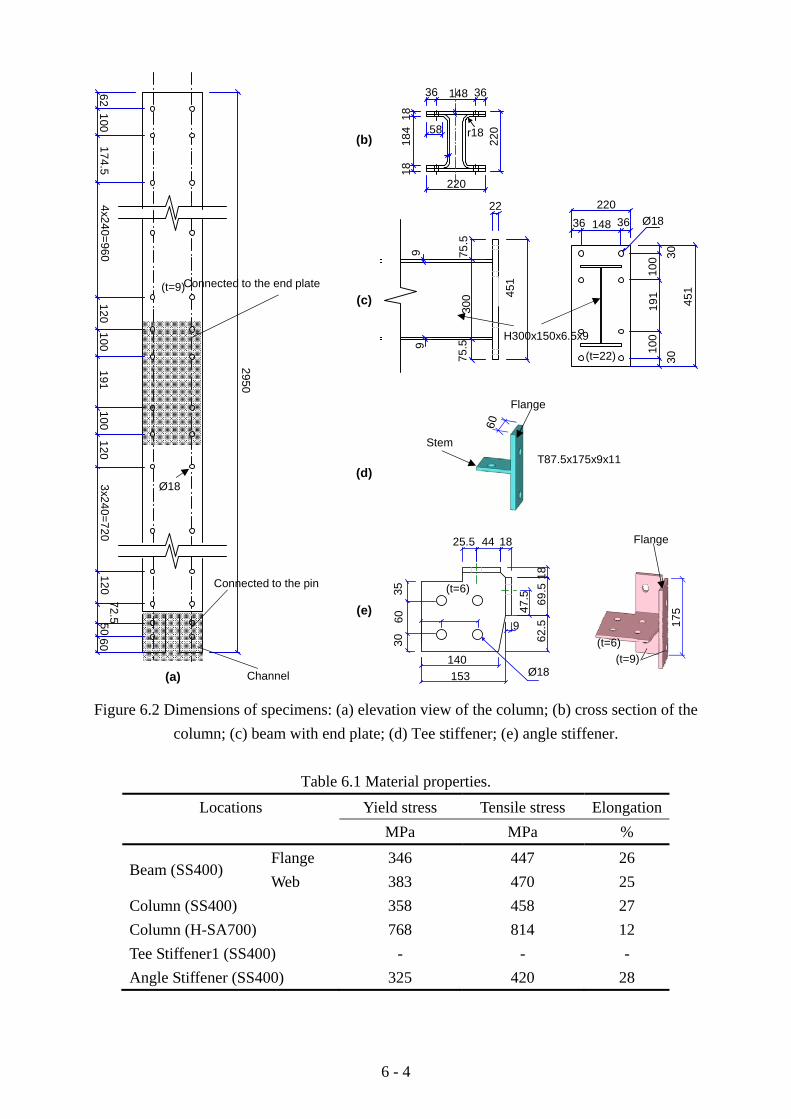
6 - 4

36 36148

220

220

184

1818

58 r18

22036 36148

451

100

100

191

3030

Ø18

(t=22)

H300x150x6.5x9

10062

174.54x240=960

120100

2950

100191

1203x240=720

12072.550

60

Connected to the end plate

Connected to the pin

(t=9)

Ø18

Channel Ø18

25.5 18

140153

9

3060

35

4447

.5 69.5

1862

.5

(t=6)

451

22

99

75.5

75.5

300

175

(t=6)

Flange

(t=9)

T87.5x175x9x11

Flange

Stem

(a)

(b)

(c)

(d)

(e)

Figure 6.2 Dimensions of specimens: (a) elevation view of the column; (b) cross section of the

column; (c) beam with end plate; (d) Tee stiffener; (e) angle stiffener.

Table 6.1 Material properties. Locations Yield stress Tensile stress Elongation

MPa MPa %

Beam (SS400) Flange 346 447 26 Web 383 470 25

Column (SS400) 358 458 27 Column (H-SA700) 768 814 12 Tee Stiffener1 (SS400) - - - Angle Stiffener (SS400) 325 420 28

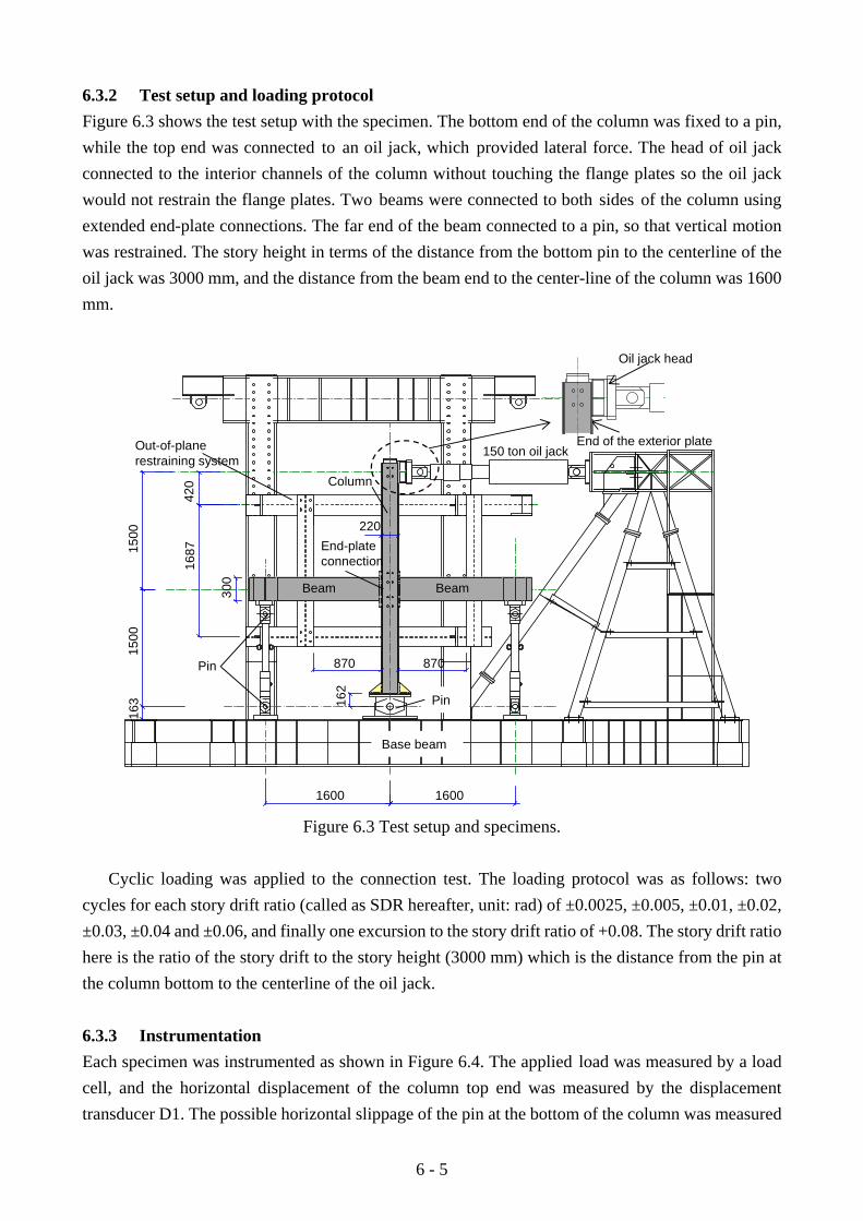
6 - 5

6.3.2 Test setup and loading protocol Figure 6.3 shows the test setup with the specimen. The bottom end of the column was fixed to a pin, while the top end was connected to an oil jack, which provided lateral force. The head of oil jack connected to the interior channels of the column without touching the flange plates so the oil jack would not restrain the flange plates. Two beams were connected to both sides of the column using extended end-plate connections. The far end of the beam connected to a pin, so that vertical motion was restrained. The story height in terms of the distance from the bottom pin to the centerline of the oil jack was 3000 mm, and the distance from the beam end to the center-line of the column was 1600 mm.

1600 1600

1500

1500

420

1687

220

870 870

162

300

Column

Beam

End-plate connection

Pin

Pin

150 ton oil jackOut-of-plane restraining system

Beam

163

End of the exterior plate

Oil jack head

Base beam

Figure 6.3 Test setup and specimens.

Cyclic loading was applied to the connection test. The loading protocol was as follows: two

cycles for each story drift ratio (called as SDR hereafter, unit: rad) of ±0.0025, ±0.005, ±0.01, ±0.02, ±0.03, ±0.04 and ±0.06, and finally one excursion to the story drift ratio of +0.08. The story drift ratio here is the ratio of the story drift to the story height (3000 mm) which is the distance from the pin at the column bottom to the centerline of the oil jack.

6.3.3 Instrumentation Each specimen was instrumented as shown in Figure 6.4. The applied load was measured by a load cell, and the horizontal displacement of the column top end was measured by the displacement transducer D1. The possible horizontal slippage of the pin at the bottom of the column was measured

6 - 6

by the displacement transducer D2. Local rotation of each beam was measured with two displacement transducers spanning 800 mm from the column face. Pi-gauge displacement transducers D7, D8 and D9, were used to monitor possible slippage between the flange plates and internal channels. Strain gauges were placed extensively on the end plate and the beam to monitor the occurrence of yielding. Five strain gauge rosettes, R1~R5, were used to measure the shear strain of the panel zone and monitor the possible plasticity. R1 was located right at the center of the panel zone of one channel, R3~R5 were at the corners, and R2 was at the center of the panel zone of the other channel (see Figure 6.4).

1 1

2 2800 800

150 150 300

60

1-1 & 2-2End plate

Rosettes on the panel zone

100

50

Measure points for the plate slippage

D1

D2

D3

D4

D5

D6

D7

D8, D9

R1 (R2)

R3 R4

R5

Load cell

Figure 6.4 Instrumentation.

6.4 Test Results and Analysis For the extended end-plate connection, deformation associated with bolt elongation and deformation of the end plate cannot be neglected [4, 5]. The built-up column has relatively small resistance to tension acting perpendicular to its flange that causes opening of the corner bents of the cold-formed interior channel and out-of-plane bending of the flange plate. Therefore, the source of story drift in the specimen can be separated into four components that are attributed to the bending of the column, bending of the beam (not including the end plates), shear deformation of the panel zone (not including the column flange deformation), and the connection zone including local distortion of the

6 - 7

column flange and the end plate in the connection (called CFEP zone hereafter). 6.4.1 Global behavior Figure 6.5 shows the deformation of the specimens at the SDR of 0.08 rad. The load versus story drift ratio relationship for each specimen is shown in Figure 6.6. In the baseline Specimen HN, slight local distortion was observed in the column flanges, and local buckling occurred in the compressive beam flanges (indicated by circles in Figure 6.5(b)). In Specimen CN, severe local distortion was observed in the column, and no local buckling was found in the beams. In the specimens that were reinforced by stiffeners, no local distortion was found in the column flanges, while the deformation was concentrated in the beams, and very severe local buckling occurred in all the beam flanges (indicated by circles in Figures 6.5(c) and (d)).

In Figure 6.6, “To Mby” is the estimated load for the beam to reach its estimated yield bending moment, and “To Mbp” is the estimated load for the beam to reach its estimated plastic bending moment. Specimen HAS had one more 0.08 rad cycle than others, just to load more at the end of the test. Specimen CN, which was the only specimen without using H-SA700 steel, had the smallest strength, but exhibited increase in strength to the end of the test. The other specimens using H-SA700 steel for their columns, presented a similar maximum strength, which 50% larger than that of Specimen CN.

CN

HN

(a) (b)

HTS

HAS

(c) (d)

Figure 6.5 Deformation of the specimens: (a) CN; (b) HN; (c) HTS; (d) HAS.

6 - 8

-180

-120

-60

0

60

120

180

-0.09 -0.06 -0.03 0 0.03 0.06 0.09

Load

(kN

)


To Mby

To Mbp

To Mbp

To Mby

-180

-120

-60

0

60

120

180

-0.09 -0.06 -0.03 0 0.03 0.06 0.09

Load

(kN

)


To Mby

To Mbp

To Mbp

To Mby

(a) (b)

-180

-120

-60

0

60

120

180

-0.09 -0.06 -0.03 0 0.03 0.06 0.09

Load

(kN

)


To Mby

To Mbp

To Mbp

To Mby

-180

-120

-60

0

60

120

180

-0.09 -0.06 -0.03 0 0.03 0.06 0.09

Load

(kN

)


To Mby

To Mbp

To Mbp

To Mby

(c) (d)

Figure 6.6 Load versus story drift ratio relationship: (a) CN; (b) HN; (c) HTS; (d) HAS.

Specifically, it is further confirmed by the strain gauges glued on the beams that the beams of Specimen CN did not yield, while those of Specimens HN, HTS and HAS yielded at a SDR of 0.029, 0.018 and 0.019 rad, respectively. Post-yield local buckling was observed on the beam flange at a SDR of about 0.06 rad in Specimen HN, about 0.04 rad in Specimen HTS and Specimen HAS. Development of local buckling at the beam end led to gradual decrease in strength. Figure 6.6 indicates strength degradation at a SDR of about 0.07 rad in Specimen HN and about 0.04 rad in Specimens HTS and HAS, which was nearly identical timing as the occurrence of local bucking noted during the test. 6.4.2 Column The columns were designed to remain elastic outside the beam-to-column connection. The strain gauges placed at the column end outside the connection region (Section 1-1 & 2-2 in the Part 1) indicated that this design goal was achieved. The yield strain, defined as the yield stress in Table 1 divided by the Young’s modulus (205,000 MPa), was not exceeded at the two sections. The column tests in Chapters 3 and 4 showed that the elastic bending stiffness of the column can be estimated by the assumption that plane sections remain plane.

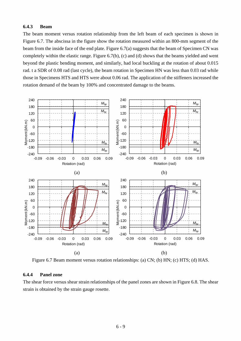
6 - 9

6.4.3 Beam The beam moment versus rotation relationship from the left beam of each specimen is shown in Figure 6.7. The abscissa in the figure show the rotation measured within an 800-mm segment of the beam from the inside face of the end plate. Figure 6.7(a) suggests that the beam of Specimen CN was completely within the elastic range. Figure 6.7(b), (c) and (d) shows that the beams yielded and went beyond the plastic bending moment, and similarly, had local buckling at the rotation of about 0.015 rad. t a SDR of 0.08 rad (last cycle), the beam rotation in Specimen HN was less than 0.03 rad while those in Specimens HTS and HTS were about 0.06 rad. The application of the stiffeners increased the rotation demand of the beam by 100% and concentrated damage to the beams.

-240

-180

-120

-60

0

60

120

180

240

-0.09 -0.06 -0.03 0 0.03 0.06 0.09

Mom

ent (

kN.m

)

Rotation (rad)

Mby

Mbp

Mbp

Mby

-240

-180

-120

-60

0

60

120

180

240

-0.09 -0.06 -0.03 0 0.03 0.06 0.09

Mom

ent (

kN.m

)

Rotation (rad)

Mby

Mbp

Mbp

Mby

(a) (b)

-240

-180

-120

-60

0

60

120

180

240

-0.09 -0.06 -0.03 0 0.03 0.06 0.09

Mom

ent (

kN.m

)

Rotation (rad)

Mby

Mbp

Mbp

Mby

-240

-180

-120

-60

0

60

120

180

240

-0.09 -0.06 -0.03 0 0.03 0.06 0.09

Mom

ent (

kN.m

)

Rotation (rad)

Mby

Mbp

Mbp

Mby

(a) (b)

Figure 6.7 Beam moment versus rotation relationships: (a) CN; (b) HN; (c) HTS; (d) HAS.

6.4.4 Panel zone The shear force versus shear strain relationships of the panel zones are shown in Figure 6.8. The shear strain is obtained by the strain gauge rosette.

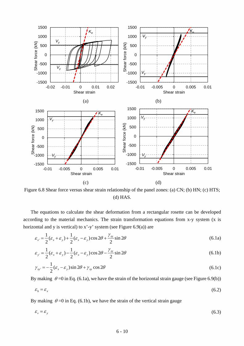
6 - 10

-1500

-1000

-500

0

500

1000

1500

-0.02 -0.01 0 0.01 0.02

Shea

r for

ce (k

N)

Shear strain

Vy

Vy

Ke

-1500

-1000

-500

0

500

1000

1500

-0.01 -0.005 0 0.005 0.01

Shea

r for

ce (k

N)

Shear strain

Vy

Vy

Ke

(a) (b)

Vy

Vy

-1500

-1000

-500

0

500

1000

1500

-0.01 -0.005 0 0.005 0.01

She

ar fo

rce

(kN

)

Shear strain

KeVy

Vy

-1500

-1000

-500

0

500

1000

1500

-0.01 -0.005 0 0.005 0.01

She

ar fo

rce

(kN

)

Shear strain

Ke

(c) (d)

Figure 6.8 Shear force versus shear strain relationship of the panel zones: (a) CN; (b) HN; (c) HTS; (d) HAS.

The equations to calculate the shear deformation from a rectangular rosette can be developed

according to the material mechanics. The strain transformation equations from x-y system (x is horizontal and y is vertical) to x’-y’ system (see Figure 6.9(a)) are

'1 1( ) ( )cos 2 sin 22 2 2

xyx x y x y

γε ε ε ε ε θ θ= + + − + (6.1a)

'1 1( ) ( ) cos 2 sin 22 2 2

xyy x y x y

γε ε ε ε ε θ θ= + − − − (6.1b)

'1 ( )sin 2 cos 22xy x y xyγ ε ε θ γ θ= − − + (6.1c)

By making θ =0 in Eq. (6.1a), we have the strain of the horizontal strain gauge (see Figure 6.9(b))

h xε ε= (6.2)

By making θ =0 in Eq. (6.1b), we have the strain of the vertical strain gauge

v yε ε= (6.3)

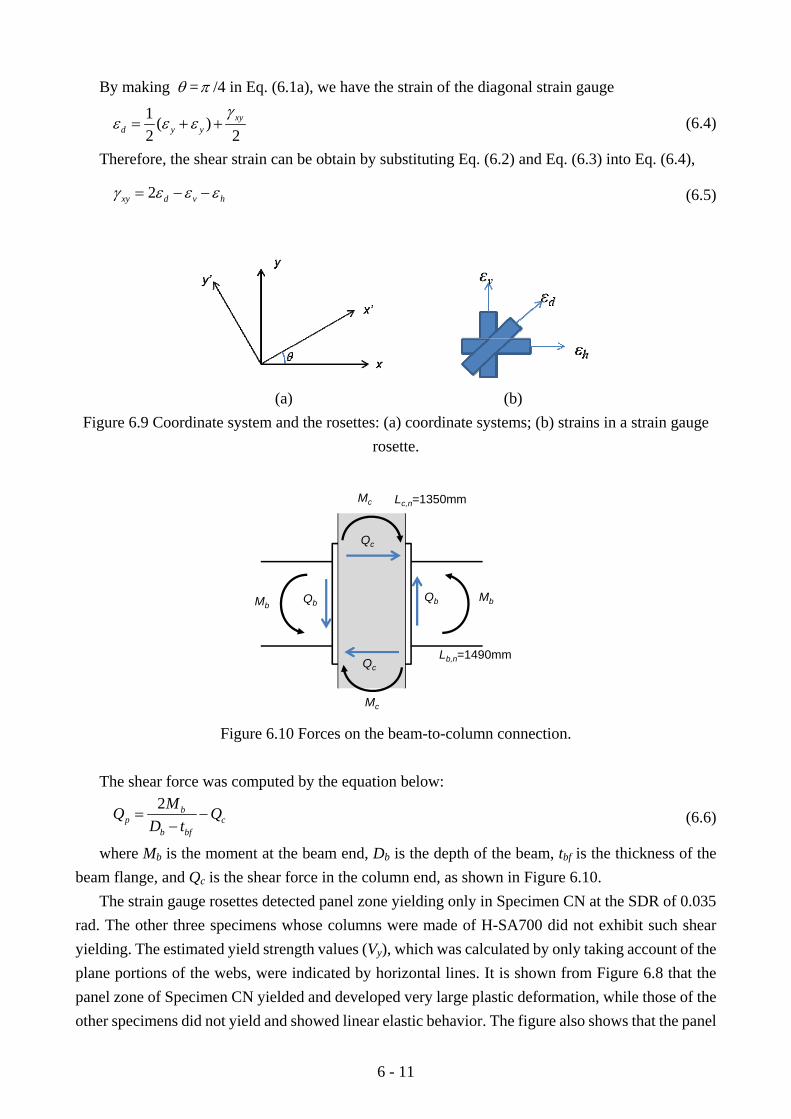
6 - 11

By making θ =π /4 in Eq. (6.1a), we have the strain of the diagonal strain gauge

1 ( )2 2

xyd y y

γε ε ε= + + (6.4)

Therefore, the shear strain can be obtain by substituting Eq. (6.2) and Eq. (6.3) into Eq. (6.4),

2xy d v hγ ε ε ε= − − (6.5)

(a) (b)

Figure 6.9 Coordinate system and the rosettes: (a) coordinate systems; (b) strains in a strain gauge rosette.

Qc

Qc

Qb Qb

Mc

Mc

MbMb

Lb,n=1490mm

Lc,n=1350mm

Figure 6.10 Forces on the beam-to-column connection.

The shear force was computed by the equation below:

2 bp c

b bf

MQ QD t

= −−

(6.6)

where Mb is the moment at the beam end, Db is the depth of the beam, tbf is the thickness of the beam flange, and Qc is the shear force in the column end, as shown in Figure 6.10.

The strain gauge rosettes detected panel zone yielding only in Specimen CN at the SDR of 0.035 rad. The other three specimens whose columns were made of H-SA700 did not exhibit such shear yielding. The estimated yield strength values (Vy), which was calculated by only taking account of the plane portions of the webs, were indicated by horizontal lines. It is shown from Figure 6.8 that the panel zone of Specimen CN yielded and developed very large plastic deformation, while those of the other specimens did not yield and showed linear elastic behavior. The figure also shows that the panel

6 - 12

zone in Specimen CN yielded when the shear force slightly exceeded its estimated yield strength, so the estimation assuming that all the shear force is resisted by the plane portions of the webs worked well with rational conservation.

The column has a flexible cold-bent portions between the channel flanges and web, and the bolted stiffeners are not as rigid as the welded ones, so one concern is whether the column can present a panel zone with clear boundaries. Hence the stiffness of the panel zone was examined. The estimated elastic stiffness [6] for the panel zone of conventional columns with welded stiffeners (continuity plates) is

GtdK pce 95.0= (6.7)

where dc is the depth of the column, tp is the total thickness of the panel plates, and G is the shear modulus of the panel zone material. The estimated elastic stiffness of the panel zone was shown in Figure 6.8 with dashed lines. For the unstiffened connections, the stiffness in the elastic range generally matches the estimated stiffness when the shear force is small (see Figure 6.8(a) and (b)). For the connections using bolted stiffeners, the shear force versus shear strain relationship curves almost coincides with the estimated dashed lines (see Figure 6.8(c) and (d)), which means that the bolted connections with bolted stiffeners still can be regarded to have a square panel zone defined by stiffeners.

6.4.5 CFEP zone and energy dissipation For Specimens HN, HTS and HAS, the panel zones were all elastic, so the plastic deformation was mainly focused in the CFEP zone and the beams. Local distortion in the CFEP zones was large in the specimens without stiffeners. Figure 6.11 shows how local tension transferred by the beam flange distorted the column flange and the end plate. Although the strength kept increasing with occurrence of local distortion on the column flanges and end plates of Specimen CN, such distortion is not favorable in an actual building where the column may be subjected to substantial compression and hence reduction of compressive strength may be detrimental to the column. The presence of the stiffeners reduced the local deformation of CFEP zone.

To give estimation about the plasticity distribution between the CFEP zone and the beams, the cumulative energy dissipated in different components was compared. The cumulative energy dissipation up to the SDR of 0.08 rad is shown in Figure 6.12. The energy dissipated by the CFEP zone was estimated by subtracting the dissipated energy of the panel zone and the beam from that of the entire specimen. For Specimen CN, most of the energy was dissipated by the connection. In the connection, although the panel zone yielded, the CFEP zone, which consisted of the column flange in the connection and the end plates of the beam, took up more energy

With the application of the stiffeners, the energy dissipated by the CFEP zone was reduced from 69% in Specimen HN to 30% in Specimen HTS, in which the energy dissipated in CFEP zone included the stiffeners, column flanges, the end plates and friction in the loading system. The energy dissipated by the beams of Specimen HTS was three times the amount by those of Specimen HN. Specimen HAS exhibited similar performance to Specimen HTS, but the Tee stiffeners were easier

6 - 13

for fabricating the connections.

(a) (b)

Figure 6.11 Local distortion in unstiffened specimens: (a) CN (b) HN.

0

40

80

120

160

200CFEP zone Beam Panel zone

CN HN HTS HAS

Ener

gy d

issi

pate

d (k

J)

69%

30%

30%

69%

Figure 6.12 Cumulative dissipation of energy up to the SDR of 0.08 rad.

6.5 Finite element analysis 6.5.1 Modeling Finite element analysis was conducted in MSC.Marc [7] for examining the yielding of the stiffened specimen (Specimen HTS), and evaluating the energy that dissipated by various connection elements in the CFEP zone. A finite element model was proposed for the beam-to-column connections based on the column models proposed in Chapters 3 and 4. Figure 6.13 shows the details of the finite element model for Specimen HTS. To reduce the computational efforts, a fiber beam element [8] was used to model the elastic portions of the beams and columns that were far (about three times of the section depth) from the beam-to-column connection. The other portions of the column and beams were modeled by eight-node reduced-integration solid elements. The beam end plates and stiffeners were also constructed with the same solid elements. Rigid links were applied to the interface between the beam elements and the portions of solid elements. A tri-linear stress strain relationship was used for the bolts [9, 10], as shown in Figure 4.9 in Chapter 4. The bolt

6 - 14

yield stress, Fyb, was 1,260 MPa and the tensile strength, Fub, was 1,400 MPa. Contact was used extensively in the model. Interaction between the mating surfaces was defined by full force transfer in the direction normal to the surface and a friction coefficient of 0.45 in the direction perpendicular to the surface. The material properties listed in Table 6.1 were used to determine the nonlinear material properties for the model, which was the same model as the one used in Chapter 3.4. The same loading protocol that used in the beam-to-column test was used for the analysis.

Bolt with pretension force

Beam element

Beam element

Solid element

Rigid link

Figure 6.13 Finite element model (HTS): (a) entire model; (b) details around the beam-to-column

connection.

6.5.2 Verification The load versus story drift ratio relationship from the finite element analysis was compared with that from the test results in Figure 6.14. The finite traced the relationship very well until very severe local buckling occurred in the beams (reaching the SDR of 0.06 rad for the first time). Although the behavior of severe local buckling was difficult to simulate accurately after reaching the SDR of 0.06 rad for the first time, the model was still able to represent the general behavior of local buckling and its corresponding strength deterioration. Therefore, the model was verified for simulation of global behaviors.

The model was further verified by comparing the local deformations. Figure 6.15 shows deformation of the model at the story drift ratio of 0.08 rad. No local distortion was observed in the column, but severe beam local buckling occurred in both the flanges and web. The model exhibited a good match with the specimen for the local buckling of the beams (see Figure 6.5(c) and Figure 6.15).

6 - 15

Load

(kN

)

Story drift ratio (rad) Figure 6.14 Comparison of load versus story drift ratio relationships

0.08

0.05

0.04

0.03

0.03

0.01

0.00

0.06

0.07

Equivalent plastic strain

Figure 6.15 Equivalent plastic strain contour and deformation (at the story drift ratio of 0.08 rad).

6.5.3 Analysis Figure 6.15 also shows the distribution of equivalent plastic strains around the beam-to-column connection. It can be seen from the figure that the area with plasticity was concentrated in the beams, end plates, and the Tee stiffeners, and large area at the beam end exhibited the plastic strain larger than 0.08 (indicated by black color in Figure 6.15).

Figure 6.16 shows the energy dissipated by the different components inside Specimen HTS. HTS (Test) is the test result, and HTS (FEM) is the result from the finite element analysis. The energy dissipated in the connection component was estimated though summing up the energy dissipated by each element. The dissipated energy in an element was calculated by the product of

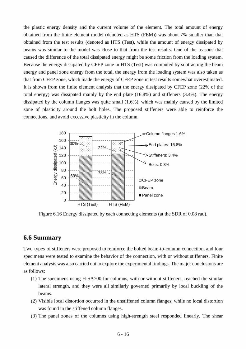
6 - 16

the plastic energy density and the current volume of the element. The total amount of energy obtained from the finite element model (denoted as HTS (FEM)) was about 7% smaller than that obtained from the test results (denoted as HTS (Test), while the amount of energy dissipated by beams was similar to the model was close to that from the test results. One of the reasons that caused the difference of the total dissipated energy might be some friction from the loading system. Because the energy dissipated by CFEP zone in HTS (Test) was computed by subtracting the beam energy and panel zone energy from the total, the energy from the loading system was also taken as that from CFEP zone, which made the energy of CFEP zone in test results somewhat overestimated. It is shown from the finite element analysis that the energy dissipated by CFEP zone (22% of the total energy) was dissipated mainly by the end plate (16.8%) and stiffeners (3.4%). The energy dissipated by the column flanges was quite small (1.6%), which was mainly caused by the limited zone of plasticity around the bolt holes. The proposed stiffeners were able to reinforce the connections, and avoid excessive plasticity in the column.

0

20

40

60

80

100

120

140

160

180

CFEP zone

Beam

Panel zone

HTS (Test) HTS (FEM)

30%

69%

22%

78%

Column flanges 1.6%

End plates: 16.8%

Stiffeners: 3.4%

Bolts: 0.3%

Ener

gy d

issi

pate

d (k

J)

Figure 6.16 Energy dissipated by each connecting elements (at the SDR of 0.08 rad).

6.6 Summary Two types of stiffeners were proposed to reinforce the bolted beam-to-column connection, and four specimens were tested to examine the behavior of the connection, with or without stiffeners. Finite element analysis was also carried out to explore the experimental findings. The major conclusions are as follows:

(1) The specimens using H-SA700 for columns, with or without stiffeners, reached the similar lateral strength, and they were all similarly governed primarily by local buckling of the beams.

(2) Visible local distortion occurred in the unstiffened column flanges, while no local distortion was found in the stiffened column flanges.

(3) The panel zones of the columns using high-strength steel responded linearly. The shear

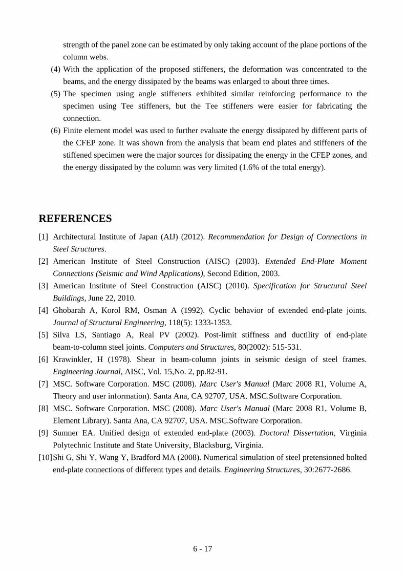
6 - 17

strength of the panel zone can be estimated by only taking account of the plane portions of the column webs.

(4) With the application of the proposed stiffeners, the deformation was concentrated to the beams, and the energy dissipated by the beams was enlarged to about three times.

(5) The specimen using angle stiffeners exhibited similar reinforcing performance to the specimen using Tee stiffeners, but the Tee stiffeners were easier for fabricating the connection.

(6) Finite element model was used to further evaluate the energy dissipated by different parts of the CFEP zone. It was shown from the analysis that beam end plates and stiffeners of the stiffened specimen were the major sources for dissipating the energy in the CFEP zones, and the energy dissipated by the column was very limited (1.6% of the total energy).

REFERENCES [1] Architectural Institute of Japan (AIJ) (2012). Recommendation for Design of Connections in

Steel Structures. [2] American Institute of Steel Construction (AISC) (2003). Extended End-Plate Moment

Connections (Seismic and Wind Applications), Second Edition, 2003. [3] American Institute of Steel Construction (AISC) (2010). Specification for Structural Steel

Buildings, June 22, 2010. [4] Ghobarah A, Korol RM, Osman A (1992). Cyclic behavior of extended end-plate joints.

Journal of Structural Engineering, 118(5): 1333-1353. [5] Silva LS, Santiago A, Real PV (2002). Post-limit stiffness and ductility of end-plate

beam-to-column steel joints. Computers and Structures, 80(2002): 515-531. [6] Krawinkler, H (1978). Shear in beam-column joints in seismic design of steel frames.

Engineering Journal, AISC, Vol. 15,No. 2, pp.82-91. [7] MSC. Software Corporation. MSC (2008). Marc User's Manual (Marc 2008 R1, Volume A,


Element Library). Santa Ana, CA 92707, USA. MSC.Software Corporation. [9] Sumner EA. Unified design of extended end-plate (2003). Doctoral Dissertation, Virginia

Polytechnic Institute and State University, Blacksburg, Virginia. [10] Shi G, Shi Y, Wang Y, Bradford MA (2008). Numerical simulation of steel pretensioned bolted

end-plate connections of different types and details. Engineering Structures, 30:2677-2686.

6 - 18

7 - 1

CHAPTER 7

Design for Local Connection of Bolted Built-up Columns

Under Concentrated Tensile Force

7.1 Overview This chapter is part of research efforts on seeking design methodology for the bolted beam-to-column connections in Chapter 6. The upper bound theorem of plastic analysis was used to derive design formulae for the strength of the bolted built-up columns under concentrated tensile load. Two possible yield patterns (collapse mechanisms) were investigated for unstiffened connections, and three possible yield patterns (collapse mechanisms) for stiffened connections. The design formulae were examined with both test results and finite element analysis.

7.2 Theoretical Study 7.2.1 Assumptions and procedures The design formula for the unstiffened connection was based on the yield-line theory for plates. The general theorem of plastic analysis, which was not limited to flat plates, was used to develop the design formula for stiffened connections. Yield line theory for plate

The yield line theory is an efficient tool to determine the plastic collapse load of a flat plate structure. This method was first introduced by Johansen [1] to analyze reinforced concrete slabs, and now has been applied successfully to both concrete slabs [2, 3] and steel plates [4, 5]. The yield line method is based on the kinematic theorem of the plastic theory of structures and gives an upper-bound solution for the collapse load [6]. Assumptions or conditions for this method are as follows:

(1) The analyzed structure is a flat, relatively thin plate. (2) The material is perfectly plastic. (3) In the assumed yield pattern, the plate is divided into undeformed plate segments by plastic

7 - 2

hinge lines (yield lines). (4) The yield pattern should be kinematically admissible over the whole plate and at the

boundaries. (5) Changes in geometry of the structure that occur at the limit load are neglected. The method has two essential parts: (1) predicting the correct yield pattern including the exact

location and orientation of each yielding line, and (2) determining a relationship between applied load and resisting moments.

There are two approaches to obtain the solution for the collapse load of a specific yield pattern: the virtual work method and the equilibrium method. Although both methods approach the same solution, the virtual work method is simpler and usually preferable for the relatively complicated yield patterns. General theorem of plastic analysis for spatial problems

The yield line theory for plates is a method simplified from the general upper bound theorem [7]. The yield line theory can be extended to a 3-D analysis by meeting the conditions of general upper bound theorem and virtual work method. The assumptions and conditions for the general upper bound theorem are almost the same as those for the yield line theory, and the only modification is that the structure can be a spatial object. Procedure

The procedure to achieve the strength of the connection under perpendicular force is as follows: (1) Assume a possible yield pattern for the connection, which should be kinematically

admissible over the local connection. (2) Assume a small arbitrary displacement (virtual displacement) on the connection. (3) Calculate the external work of the local connection as the load passes through the small

displacement. (4) Calculate the internal work of the local connection, which is generated by the plastic

rotation or translation along the assumed yield lines to accommodate the small displacement.

(5) Set the external work to be equal to the internal work, and obtain the load to form the assumed yield pattern.

(6) Repeat steps (1) ~ (5) to obtain the loads for all the assumed yield patterns, and choose the smallest load as the strength of the local connection.

7.2.2 Unstiffened Connection Figure 7.1 shows the forces on the column flanges in end-plate beam-to-column connections. The bending moment from the beam can be taken as concentrated tensile or compressive forces from the beam flanges, as shown in Figure 7.1(a) and (b). Tf is the tensile force delivered to the column flange when the beam reaches its ultimate strength. To simplify the estimation on the strength of unstiffened bolted built-up column under perpendicular tensile force, the small resistance of the exterior plate against the perpendicular force is neglected, and the local tensile force is assumed to be equally shared by the two channels. The tensile force that acts on one channel is 0.5Tf through the bolts, as

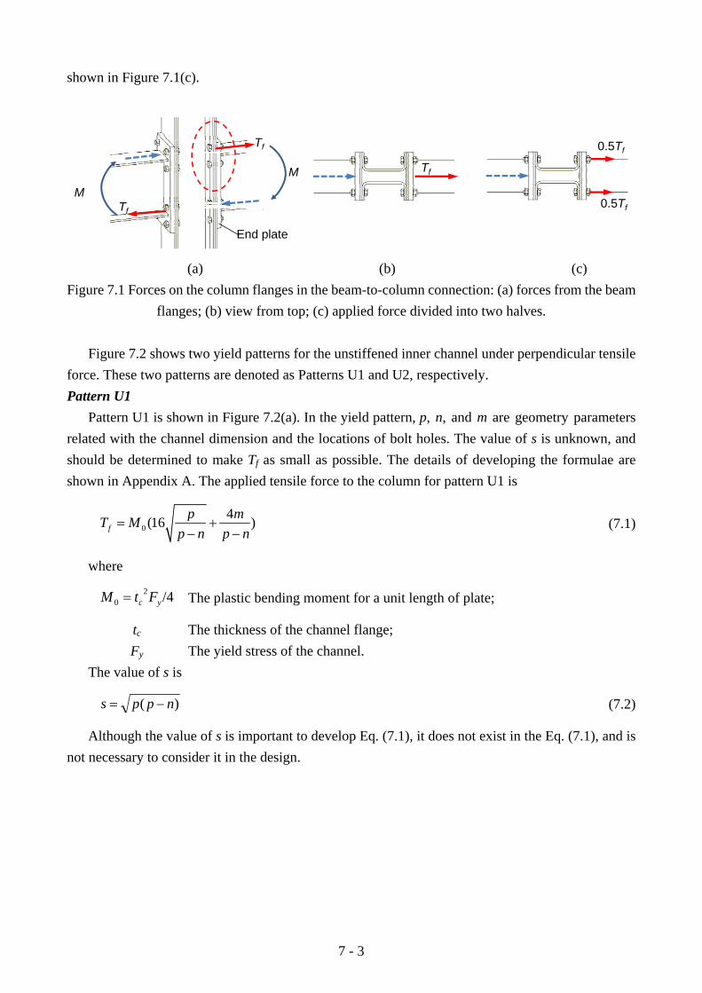
7 - 3

shown in Figure 7.1(c).

Tf

Tf

Tf

End plate

0.5Tf

0.5Tf

M

M

(a) (b) (c) Figure 7.1 Forces on the column flanges in the beam-to-column connection: (a) forces from the beam

flanges; (b) view from top; (c) applied force divided into two halves.

Figure 7.2 shows two yield patterns for the unstiffened inner channel under perpendicular tensile force. These two patterns are denoted as Patterns U1 and U2, respectively. Pattern U1

Pattern U1 is shown in Figure 7.2(a). In the yield pattern, p, n, and m are geometry parameters related with the channel dimension and the locations of bolt holes. The value of s is unknown, and should be determined to make Tf as small as possible. The details of developing the formulae are shown in Appendix A. The applied tensile force to the column for pattern U1 is

04(16 )f

p mT Mp n p n

= +− −

(7.1)

where

/420 yc FtM = The plastic bending moment for a unit length of plate;

tc The thickness of the channel flange; Fy The yield stress of the channel.

The value of s is

)( npps −= (7.2)

Although the value of s is important to develop Eq. (7.1), it does not exist in the Eq. (7.1), and is not necessary to consider it in the design.

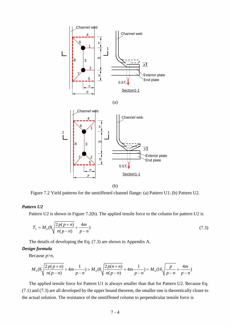
7 - 4

4

1

8 3

2

57

6

np

s

m

s

x

0.5Tf


Channel web

Channel web

1

Section1-1

(a)

4

1

8 3

25

7

6

np

s

m

s

0.5Tf


Channel web

Channel web

1 1

Section1-1

x

(b)

Figure 7.2 Yield patterns for the unstiffened channel flange: (a) Pattern U1; (b) Pattern U2.

Pattern U2 Pattern U2 is shown in Figure 7.2(b). The applied tensile force to the column for pattern U2 is

02 ( ) 4(8 )

( )fp p n mT M

n p n p n+

= +− −

(7.3)

The details of developing the Eq. (7.3) are shown in Appendix A. Design formula

Because p>n,

0 0 02 ( ) 1 2 ( ) 1 4(8 4 ) (8 4 ) (16 )

( ) ( )p p n p n n p mM m M m M

n p n p n n p n p n p n p n+ +

+ > + = +− − − − − −

The applied tensile force for Pattern U1 is always smaller than that for Pattern U2. Because Eq. (7.1) and (7.3) are all developed by the upper bound theorem, the smaller one is theoretically closer to the actual solution. The resistance of the unstiffened column to perpendicular tensile force is

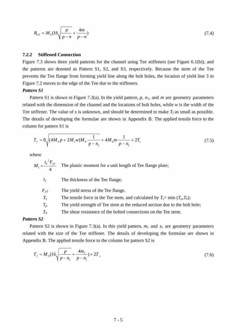
7 - 5

04(16 )UT

p mR Mp n p n

= +− −

(7.4)

7.2.2 Stiffened Connection Figure 7.3 shows three yield patterns for the channel using Tee stiffeners (see Figure 6.1(b)), and the patterns are denoted as Pattern S1, S2, and S3, respectively. Because the stem of the Tee prevents the Tee flange from forming yield line along the bolt holes, the location of yield line 3 in Figure 7.2 moves to the edge of the Tee due to the stiffeners. Pattern S1

Pattern S1 is shown in Figure 7.3(a). In the yield pattern, p, n1, and m are geometry parameters related with the dimension of the channel and the locations of bolt holes, while w is the width of the Tee stiffener. The value of s is unknown, and should be determined to make Tf as small as possible. The details of developing the formulae are shown in Appendix B. The applied tensile force to the column for pattern S1 is

sf Tnp

mMnp

MwMpMT 2141)24(81

01

010 +−

+−

+= (7.5)

where 2

1 4T yTt F

M = The plastic moment for a unit length of Tee flange plate;

Tt The thickness of the Tee flange;

FyT The yield stress of the Tee flange. Ts The tensile force in the Tee stem, and calculated by Ts= min (Tp,Tb); Tp The yield strength of Tee stem at the reduced section due to the bolt hole; Tb The shear resistance of the bolted connections on the Tee stem.

Pattern S2 Pattern S2 is shown in Figure 7.3(a). In this yield pattern, m1 and s1 are geometry parameters

related with the size of the Tee stiffener. The details of developing the formulae are shown in Appendix B. The applied tensile force to the column for pattern S2 is

sf Tnp

mnp

pMT 2)416(1

1

10 +

−+

−= (7.6)

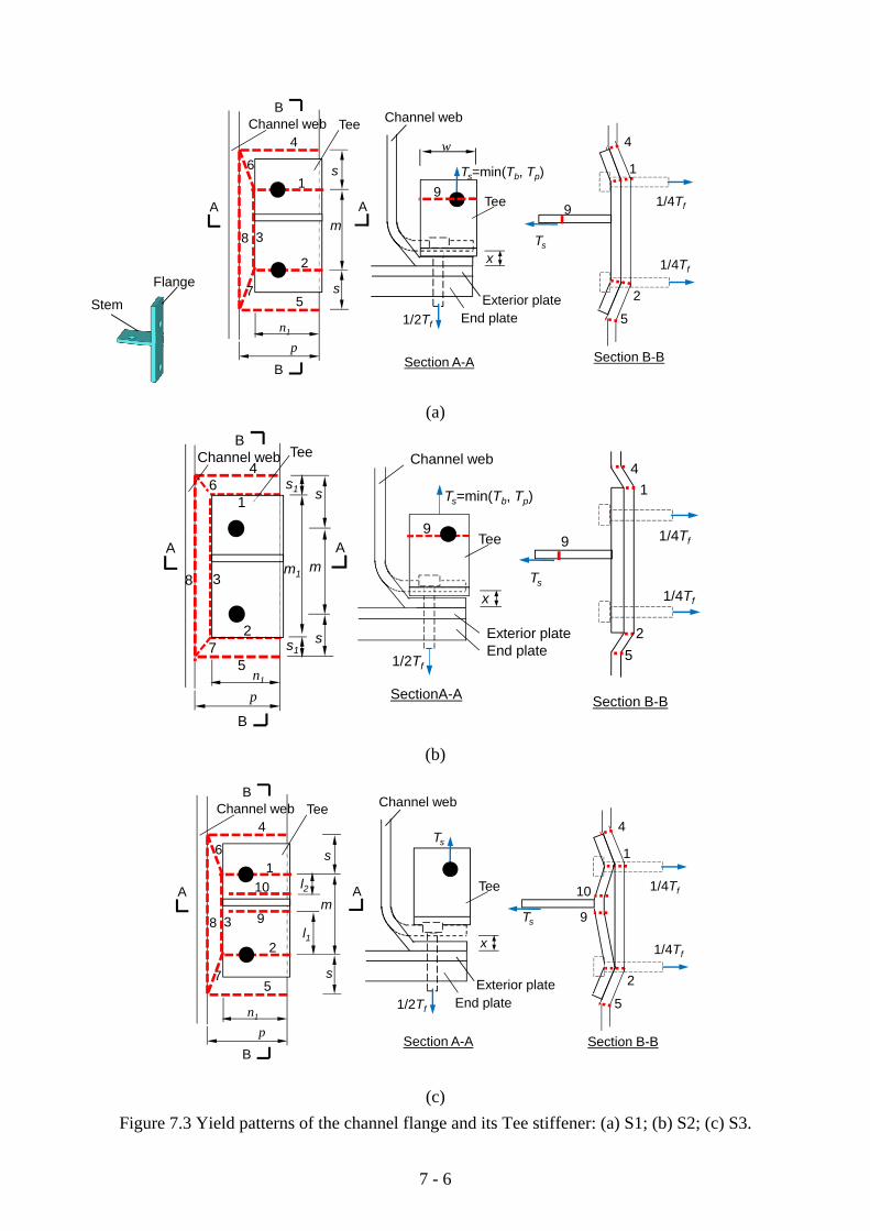
7 - 6

FlangeStem

4

1

8 3

2

57

n1

p

s

m

s

TeeChannel web

A A

6


Channel web

Tee

Section A-A

w

9Ts=min(Tb, Tp)

1/2Tf

Ts

1/4Tf

4

1/4Tf

B

BSection B-B

5

1

2

9

x

(a)

4

57

6

n1

p

s

m

s Exterior plateEnd plate

Channel web

Tee

TeeChannel web

1/2Tf

SectionA-A

m1

s1

s1

Ts=min(Tb, Tp)

9

Ts

1/4Tf

4

1/4Tf

Section B-B

1

2

9

5

A A

B

B

b8 3

2

1

x

(b)

4

1

8 3

2

57

n1

p

s

m

s

TeeChannel web

A A

6


Channel web

Tee

Section A-A

1/2Tf

Ts

1/4Tf

4

1/4Tf

B

BSection B-B

5

1

2

9

x

10

9

10

l1

l2

Ts

(c) Figure 7.3 Yield patterns of the channel flange and its Tee stiffener: (a) S1; (b) S2; (c) S3.

7 - 7

Pattern S3 Pattern S3 is shown in Figure 7.3(c). In this yield pattern, l1 and l1 are geometry parameters

related with the size of the Tee stiffener and locations of bolt holes. The details of developing the formulae are shown in Appendix B. The applied tensile force to the column for pattern S3 is

)11(4141)24(821

11

01

010 llwM

npmM

npMwMpMTf ++

−+

−+= (7.7)

Design formula Any one of the three yield patterns is possible to have the smallest resistance, as the parameters

of Tee stiffener changes. By comparing the Eq. (7.5), (7.6) and (7.7), the effect of parameters on the yield pattern can be obtained.

If M1 or w increases, the resistances of Pattern S1 and Pattern S3 become larger, while that of Pattern S2 does not change. M1 is affected by the thickness and yield stress of the Tee flange, and w is the width of the Tee flange. If the Tee flange strong enough, Pattern S2 will have the smallest resistance.

Both of Eq. (7.5) and (7.7) have three parts in the formula, and the only difference between these two equations is the third part. The value of the third part in Eq. (7.5) is determined by the equivalent yield strength of the Tee stem, while that in Eq. (7.7) determined by the strength of the Tee flanges. If Pattern S1 has smaller resistance, we have

11 2

1 12 ( )sT M wl l

< + (7.8)

If the condition in Eq. (7.8) is met, Pattern S1 has smaller resistance than Pattern S3. If not met, Pattern S3 has the smaller resistance.

The resistance of the stiffened column to perpendicular tensile force is

1 2 3min( , , )ST ST ST STR R R R= (7.9)

where 1STR is the resistance computed by Eq.(7.5), 2STR by Eq.(7.6), and 3STR by Eq.(7.7).

7.3 Verification and Discussions The existing experimental results and finite element analysis in both Chapters 5 and 6 were used to examine the proposed formulae Eq. (7.4) for unstiffened connections and Eq. (7.9) for stiffened connections. 7.3.1 Local tension test

Eq. (7.4) was used to estimate the strength of the unstiffened column under perpendicular tensile force in local tension test. Figure 5.7 shows that the proposed formula was slightly conservative (by 5%~10%) for estimating the strength at formation of the yield pattern (collapse mechanism). The

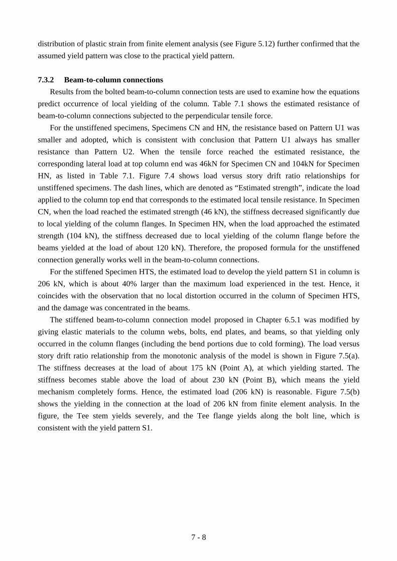
7 - 8

distribution of plastic strain from finite element analysis (see Figure 5.12) further confirmed that the assumed yield pattern was close to the practical yield pattern.

7.3.2 Beam-to-column connections

Results from the bolted beam-to-column connection tests are used to examine how the equations predict occurrence of local yielding of the column. Table 7.1 shows the estimated resistance of beam-to-column connections subjected to the perpendicular tensile force.

For the unstiffened specimens, Specimens CN and HN, the resistance based on Pattern U1 was smaller and adopted, which is consistent with conclusion that Pattern U1 always has smaller resistance than Pattern U2. When the tensile force reached the estimated resistance, the corresponding lateral load at top column end was 46kN for Specimen CN and 104kN for Specimen HN, as listed in Table 7.1. Figure 7.4 shows load versus story drift ratio relationships for unstiffened specimens. The dash lines, which are denoted as “Estimated strength”, indicate the load applied to the column top end that corresponds to the estimated local tensile resistance. In Specimen CN, when the load reached the estimated strength (46 kN), the stiffness decreased significantly due to local yielding of the column flanges. In Specimen HN, when the load approached the estimated strength (104 kN), the stiffness decreased due to local yielding of the column flange before the beams yielded at the load of about 120 kN). Therefore, the proposed formula for the unstiffened connection generally works well in the beam-to-column connections.

For the stiffened Specimen HTS, the estimated load to develop the yield pattern S1 in column is 206 kN, which is about 40% larger than the maximum load experienced in the test. Hence, it coincides with the observation that no local distortion occurred in the column of Specimen HTS, and the damage was concentrated in the beams.

The stiffened beam-to-column connection model proposed in Chapter 6.5.1 was modified by giving elastic materials to the column webs, bolts, end plates, and beams, so that yielding only occurred in the column flanges (including the bend portions due to cold forming). The load versus story drift ratio relationship from the monotonic analysis of the model is shown in Figure 7.5(a). The stiffness decreases at the load of about 175 kN (Point A), at which yielding started. The stiffness becomes stable above the load of about 230 kN (Point B), which means the yield mechanism completely forms. Hence, the estimated load (206 kN) is reasonable. Figure 7.5(b) shows the yielding in the connection at the load of 206 kN from finite element analysis. In the figure, the Tee stem yields severely, and the Tee flange yields along the bolt line, which is consistent with the yield pattern S1.

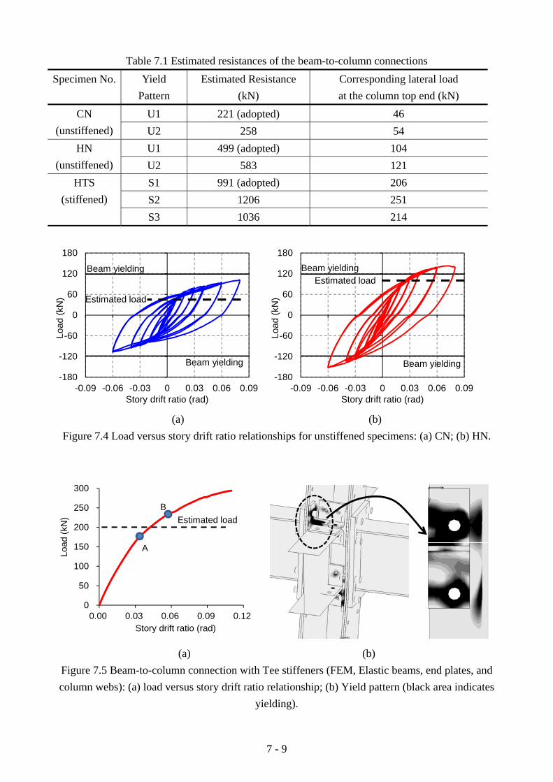
7 - 9

Table 7.1 Estimated resistances of the beam-to-column connections Specimen No. Yield

Pattern Estimated Resistance

(kN) Corresponding lateral load at the column top end (kN)

CN (unstiffened)

U1 221 (adopted) 46 U2 258 54

HN (unstiffened)

U1 499 (adopted) 104 U2 583 121

HTS (stiffened)

S1 991 (adopted) 206 S2 1206 251 S3 1036 214

-180

-120

-60

0

60

120

180

-0.09 -0.06 -0.03 0 0.03 0.06 0.09

Load

(kN

)


Estimated load

Beam yielding

Beam yielding

-180

-120

-60

0

60

120

180

-0.09 -0.06 -0.03 0 0.03 0.06 0.09

Load

(kN

)


Estimated loadBeam yielding

Beam yielding

(a) (b)

Figure 7.4 Load versus story drift ratio relationships for unstiffened specimens: (a) CN; (b) HN.

0

50

100

150

200

250

300

0.00 0.03 0.06 0.09 0.12

Estimated load

A

B


Load

(kN

)

(a) (b) Figure 7.5 Beam-to-column connection with Tee stiffeners (FEM, Elastic beams, end plates, and column webs): (a) load versus story drift ratio relationship; (b) Yield pattern (black area indicates

yielding).

7 - 10

7.4 Summary The upper bound theorem of plastic analysis was used to derive design equations for the built-up column subjected to local tension. The equations accounted for local tension failure, which dictates the column-side limit state in the bolted beam-to-column connection. The major conclusions are as follows:

(1) By comparing the proposed estimation formulae of the two yield patterns for the unstiffened connections, one of them was found to be smaller unconditionally and thus controls.

(2) Three yield patterns were investigated for the stiffened connection using Tee stiffeners, the corresponding estimation formulae were developed. The controlling yield patterns differ according to the dimensions of the stiffeners.

(3) The results and finite element analysis were used to examine the proposed formulas. The proposed formulas and mechanisms agreed reasonably with the results from tests and finite element analysis.

REFERENCES [1] Johansen KW (1972). Yield-line Formulae for Slabs. Cement and Concrete Association,

London, England. [2] Jones LL, Wood RH (1967). Yield-line Analysis of Slabs. American Elsevier, New York. [3] Park R and Gamble WL (1980). Reinforced Concrete Slabs. Wiley Interscience, New York. [4] Srouji R, Kukreti AR, Murray TM (1983). Yield-line analysis of end-plate connections with

bolt force predictions. Research Report No.FSEL/MBMA 83-05, Fears Structural Engineering Laboratory, School of Civil Engineering and Environmental Science, University of Okalahoma, Norman, Okalahoma.

[5] Sumner EA. (2003). Unified design of extended end-plate. Doctoral Dissertation, Virginia Polytechnic Institute and State University, Blacksburg, Virginia.

[6] Bauer D, Redwood RG (1987). Numerical yield line analysis. Computers and Structures, 26(04): 587-596.

[7] Chen WF, Han DJ. (1988). Plasticity for Structural Engineers. Springer-Verlag, New York.

7 - 11

Appendix A. Formulae for Local Tension of Unstiffened Connection A.1 Pattern U1

Pattern U1 is shown in Figure 7.2(a). The applied tensile force to one channel flange is 0.5Tf . For any virtual displacement x perpendicular to the column flange, we have Internal work

Line 1 and Line 2: sxnMW 012 2=

Line 3 and Line 8: np

xsmMW−

+= )(2 038

Line 4 and Line 5: sxpMW 045 2=

Line 6 and Line 7: ⎥⎦

⎤⎢⎣

⎡−

+−=np

xssxnpMW )(2 067

Where M0 is the plastic bending moment for a unit length of plate, 20 / 4c yM t F= , tc is the

thickness of the channel, Fy is the yield stress of the channel. The total internal work

xnp

snp

ms

pMWWWWWin ⋅−

+−

+=+++= )141214(067453812

The total external work

xTW fe ⋅= 5.0

According to the principle of virtual work, ein WW = , we have

)141214(5.0 0 nps

npm

spMTf −

+−

+= )128(0 npm

nppM

−+

−≥

We seek the minimum value for Tf. When and only when ( )npssp −= 44 , we can get the minimum Tf, so we have

)( npps −=

)416(0 npm

nppMTf −

+−

=

A.2 Pattern U2

Pattern U2 is shown in Figure 7.2(b). For any virtual displacement x perpendicular to the column flange, we have

7 - 12

Internal work

Line 1 and Line 2: )(2 012 nxs

sxnMW +=

Line 3 and Line 8: np

xsmMW−

+= )(2 038



⎤⎢⎣

⎡−

+−=np

xssxnpMW )(2 067

The principle of virtual work leads to

)12141214(5.0 0 ns

nps

npm

spMTf +

−+

−+=

)12)()(24(0 np

mnpnnppM

−+

−+

≥

When and only when)(

214npn

npss

p−+

= , we can get the minimum Tf, so we have

npnppns

+−

=)(2

)14)()(28(0 np

mnpnnppMT f −

+−+

=

7 - 13

Appendix B. Formulae for Local Tension of Stiffened Connection B.1 Pattern S1

Pattern S1 is shown in Figure 7.3(a). The tension force in the Tee stem reaches its equivalent yield force (Ts) as long as the reduced section due to bolt hole yields or the tensile force reaches the friction shear resistance.

Ts=min(Tp,Tb) Where Tp is the yield strength of the reduced section due to bolt hole, and Tb is the shear resistance

of the bolted connection. For any virtual displacement x perpendicular to the column flange, taking one of the channels for

the analysis, we have Internal work

Line 1 and Line 2 (including the Tee): sxwM

sxnMW 11012 22 +=

Line 3 and Line 8: 1

038 )(2np

xsmMW−

+=



⎤⎢⎣

⎡−

+−=1

1067 )(2np

xssxnpMW

Line 9: xTW s=9


sf Tsnp

Mnp

mMs

wMpMT +−

+−

++=1

01

01014121)24(5.0

sTnp

mMnp

MwMpM +−

+−

+≥1

01

0101214)24(2

Because Tf is an upper bound load, the minimum Tf is closer to the true load. Only

when snp

Ms

wMpM1

010141)24(−

=+ , we can get the minimum Tf, so we have

0

110

2))(2(

MnpwMpMs −+

=

sf Tnp

mMnp

MwMpMT 2141)24(81

01

010 +−

+−

+=

B.2 Pattern S2

7 - 14

Pattern S2 is shown in Figure 7.3(b). For any virtual displacement x perpendicular to the column flange, taking one of the channels for the analysis, we have

Internal work


1012 2sxnMW =


11038 )(2np

xsmMW−

+=


045 2sxpMW =


⎤⎢⎣

⎡−

+−=1

11

1067 )(2np

xssxnpMW

Line 9: xTW s=9

Where M0 is the plastic bending moment for a unit length of plate, 20 / 4c yM t F= , tc is the

thickness of the channel, Fy is the yield strength of the channel. The total internal work

xTxnp

snp

ms

pMWWWWWW sin +⋅−

+−

+=++++= )141214(11

11

0967453812


sf Tnp

snp

ms

pMT +−

+−

+= )141214(5.01

11

11

0

sTnp

mnp

pM +−

+−

≥ )128(1

11

0

When and only when1

11

1414np

ss

p−

= , we can get the minimum Tf, so we have

)( 11 npps −=

sf Tnp

mnp

pMT 2)416(1

1

10 +

−+

−=

B.3 Pattern S3 Pattern S3 is shown in Figure 7.3(c). For any virtual displacement x perpendicular to the column

flange, taking one of the channels for the analysis, we have Internal work

Line 1 and Line 2 (including the Tee): )2(221

11012 lx

lx

sxwM

sxnMW +++=

7 - 15


038 )(2np

xsmMW−

+=



⎤⎢⎣

⎡−

+−=1

1067 )(2np

xssxnpMW

Line 9 and Line 10: )(21

110,9 lx

lxwMW +=


)11(214121)24(5.021

11

01

010 llwMs

npM

npmM

swMpMTf ++

−+

−++=

)11(21214)24(221

11

01

010 llwM

npmM

npMwMpM ++

−+

−+≥

When and only when snp

Ms

wMpM1

010141)24(−

=+ , we can get the minimum Tf, so we have

0

110

2))(2(

MnpwMpMs −+

=

)11(4141)24(821

11

01

010 llwM

npmM

npMwMpMTf ++

−+

−+=

7 - 16

8 - 1

CHAPTER 8

Summary and Conclusions

8.1 Summary and Conclusions H-SA700 is a new ultra-high strength steel with a specified yield strength range of 700 to 900 MPa, which is about three times the yield strength of the conventional steel. This steel achieves very high strength without significantly increasing alloying elements and without introducing intensive heat treatment, so it is more environmentally friendly (because of lower discharge of CO2) and more suitable for mass production than conventional high-strength steel.

The research target of this dissertation is to develop a structural system that (1) minimizes energy consumption during manufacturing, fabrication, and construction, (2) maximizes reusability and recyclability, (3) enables continuous use after major earthquakes, and (4) most notably, and unlike previous development efforts focused on ultra-high strength steel, targets low- to mid-rise buildings (not special structures) in which the majority of structural steel is consumed. About 95% of the floor area constructed every year in Japan belongs to the buildings of no more than ten stories.

In order to achieve these goals, all members in the proposed system are connected by only bolts and no welds, so that all the components can be replaced, reused, and recycled. The column pattern, which is built up from H-SA700 steel plates, either flat or cold bent, using bolts exclusively and no welds, is adopted. The columns are intended to have sufficiently large strength to keep elastic under very rare earthquake events, which enable continuous use of the buildings even after very rare earthquake events.

This dissertation consists of eight chapters. Chapter 1 is the background of this study, and Chapter 8 is the summary and conclusions. Chapters 2 to 7 constitute the main part of the dissertation: (1) column pattern and the prototype building; (2) flexural behavior of the bolted built-up columns; (3) column behavior subjected to combined axial force and cyclic lateral force; (4) behavior of unstiffened built-up column subjected to concentrated perpendicular force; (5) behavior of bolted beam-to-column connections; and (6) design for local connection of the column under concentrated tensile force. The mayor findings obtained from the six chapters are summarized as follows.

8 - 2

Analysis on Feasibility of Prototype building system In Chapter 2, preliminary details of the building system using ultra-high-strength steel are examined, and the performance of prototype structure is evaluated. The main conclusions are as follows:

(1) A bolted built-up column pattern was proposed by balancing the advantages of closed sections and open sections, and mechanical performance with feasible fabrication details was identified.

(2) Three braced frame were designed to evaluate the seismic performance of the proposed structural system. One was a conventional braced frame, and the other two were the candidate prototype structures using ultra-strength-steel for the columns. One candidate prototype frame used flexible columns of small section, while the other used strong columns of doubled strength.

(3) Modal analysis was carried out to examine the dynamic characteristics of each frame. The three frames exhibited similar modal shapes, with slightly different periods. The first-mode period of the frame with flexible columns was about 15% larger than the conventional frame, while that of the frame with strong columns was basically the same as the conventional frame.

(4) Static nonlinear pushover analyses were conducted to investigate the capacity and damage of the frames. By using high-strength steel only in the columns, the maximum roof drift to keep the columns and beams elastic was increased by 57% in the frame using strong columns, and 129% in the frame using flexible columns.

(5) Incremental Dynamic Analysis (IDA) was carried out to evaluate the seismic performance of the frames. The frame using flexible columns exhibited a larger maximum story drift for the pulse-like ground motion, although educed the residual deformation by 60%. The frame using strong column was superior to reduce the maximum story drift (reduced by 60%) and the residual deformation (reduced by 83% to 94%), and therefore, was adopted as the prototype frame.

Flexural behavior of bolted built-up columns In Chapter 3, the flexural performance of proposed bolted built-up column was investigated with both static cyclic tests and finite element simulation. Three specimens, H-120 made of ultra-high strength steel, S-120 made of conventional steel, and H-360 made of ultra-high strength steel with a sparse bolt arrangement, were conducted. Nonlinear finite element analysis was presented to generalize the findings. The following conclusions were made based on the experiment and finite element analysis:

(1) The elastic bending deformation of the column was more than doubled by using the high-strength steel. The elastic bending stiffness of the bolted built-up column can be estimated based on the assumption that the plane sections remain plane. Slippage was not observed before severe local buckling.

(2) The yield bending moment and maximum bending moment of the built-up column can be estimated reasonably by the yield bending moment and the plastic bending moment of the net area of the section with bolt holes. Specimens H-120 and S-120 had a similar maximum to

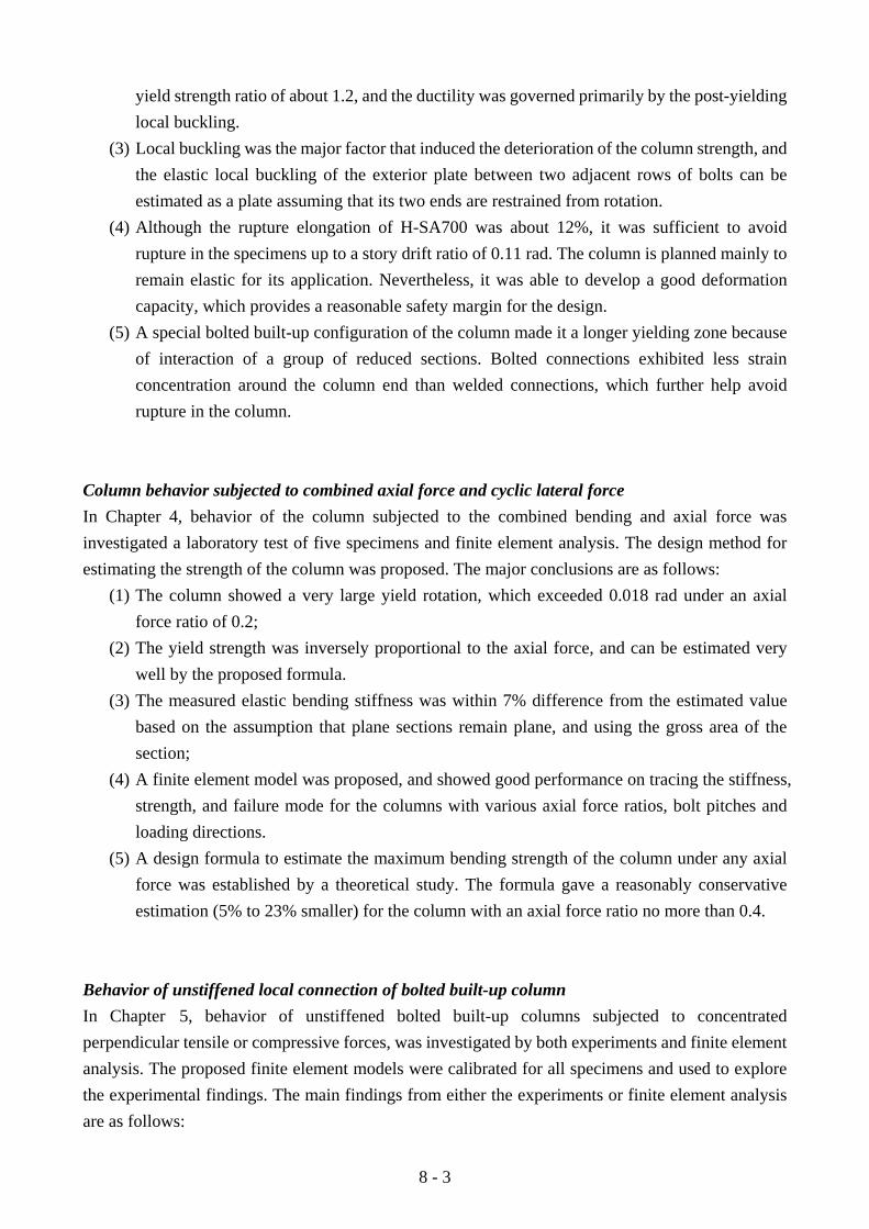
8 - 3

yield strength ratio of about 1.2, and the ductility was governed primarily by the post-yielding local buckling.

(3) Local buckling was the major factor that induced the deterioration of the column strength, and the elastic local buckling of the exterior plate between two adjacent rows of bolts can be estimated as a plate assuming that its two ends are restrained from rotation.

(4) Although the rupture elongation of H-SA700 was about 12%, it was sufficient to avoid rupture in the specimens up to a story drift ratio of 0.11 rad. The column is planned mainly to remain elastic for its application. Nevertheless, it was able to develop a good deformation capacity, which provides a reasonable safety margin for the design.

(5) A special bolted built-up configuration of the column made it a longer yielding zone because of interaction of a group of reduced sections. Bolted connections exhibited less strain concentration around the column end than welded connections, which further help avoid rupture in the column.

Column behavior subjected to combined axial force and cyclic lateral force In Chapter 4, behavior of the column subjected to the combined bending and axial force was investigated a laboratory test of five specimens and finite element analysis. The design method for estimating the strength of the column was proposed. The major conclusions are as follows:

(1) The column showed a very large yield rotation, which exceeded 0.018 rad under an axial force ratio of 0.2;

(2) The yield strength was inversely proportional to the axial force, and can be estimated very well by the proposed formula.

(3) The measured elastic bending stiffness was within 7% difference from the estimated value based on the assumption that plane sections remain plane, and using the gross area of the section;

(4) A finite element model was proposed, and showed good performance on tracing the stiffness, strength, and failure mode for the columns with various axial force ratios, bolt pitches and loading directions.

(5) A design formula to estimate the maximum bending strength of the column under any axial force was established by a theoretical study. The formula gave a reasonably conservative estimation (5% to 23% smaller) for the column with an axial force ratio no more than 0.4.

Behavior of unstiffened local connection of bolted built-up column In Chapter 5, behavior of unstiffened bolted built-up columns subjected to concentrated perpendicular tensile or compressive forces, was investigated by both experiments and finite element analysis. The proposed finite element models were calibrated for all specimens and used to explore the experimental findings. The main findings from either the experiments or finite element analysis are as follows:

8 - 4

For the unstiffened column subjected to concentrated tensile force: (1) The column exhibited significant strength increase after the yield pattern formed. Since the

out-of-plane deformation increases fast when yield pattern forms, stiffeners is needed to limit its out-of-plane deformation and plasticity when the load demand is larger than the estimated strength

(2) The proposed formula based on yield line theory was slightly conservative (by 5%~10%) for estimating the strength at the formation of the yield pattern.

For the unstiffened column subjected to concentrated compressive force: (1) Although the column yield under a small load, the strength kept increasing after yielding,

the observed maximum strength was five times the yield strength. The strength was not affected much by simply enlarging the compression length (25 mm to 80 mm).

(2) The vertical displacement of the column after yielding was significantly cut by half through stiffening the webs from local distortion. Stiffeners that can increase the out-of-plane stiffness of the web, may be effective to reinforce the column subjected to concentrated compressive force.

Behavior of bolted beam-to-column connections In Chapter 6, two stiffeners were proposed to reinforce the proposed bolted beam-to-column connections and four specimens were tested to examine the behavior of the connections, with or without stiffeners. Finite element analysis was carried out to supplement the experimental findings. Major conclusions are as follows:

(1) The specimens using H-SA700 for columns, with or without stiffeners, reached the similar lateral strength, and the strength was governed by local buckling of the beams.

(2) Visible local distortion occurred in the unstiffened column flanges, while no local distortion was found in the stiffened column flanges.

(3) All the panel zones of the columns using high-strength steel responded linearly. The shear strength of the panel zone can be estimated by taking only the plane portions of the column webs into account.

(4) With the application of the proposed stiffeners, the deformation was concentrated to the beams, and the energy dissipated by the beams was enlarged to about three times.

(5) Specimen HAS (using angle stiffeners) exhibited similar reinforcing performance to Specimen HTS (using Tee stiffeners), but Tee stiffeners were easier for fabricating the connection.

(6) Finite element model was used to further evaluate the energy dissipated by different parts of the CFEP zone. It was shown from the analysis that the beam end plates and stiffeners of the stiffened specimen were the major sources for dissipating the energy in the CFEP zones, while the energy dissipated by the column was very limited (1.6% of the total energy).

Design for local connection of columns under perpendicular tensile force In Chapter 7, theoretical studies based on the upper bound theorem were conducted for establishing

8 - 5

the design for the bolted beam-to-column connection under perpendicular tensile force. The major conclusions are as follows:

(1) By comparing the proposed estimation formulae of the two yield patterns for the unstiffened connections, one of the patterns is always smaller and thus controls.

(2) Three yield patterns were investigated for stiffened connection using Tee stiffeners, the corresponding estimation formulae were developed, and the controlling yield pattern differs as the dimensions of the stiffeners changes. The application condition for each pattern was presented.

(3) Experimental results and finite element analysis from earlier chapters were used to examine the proposed formulae. The proposed formulae and mechanisms agreed with the results from either finite element analysis or tests.

8.2 Future Work The study presented in the dissertation shall be extended to develop the details of design for the proposed built-up columns and related connection components, such as column base connections, column splices, and bracing connections. Other issues, such as fire resistance, health monitoring of the structural components, are also important for the future use of the structural system.

Column base

Bolted column bases are being developed for the prototype structure. Embedded column bases are difficult to remove or reuse, so exposed column bases are considered. As an illustration, Figure 8.1 shows conceptual views of three exposed bolted column bases to explore for the next-step research.

(a) (b) (c) Figure 8.1 Conceptual views of bolted column bases: (a) End-plate column base; (b)

Extended-exterior-plate column base; (c) Two-bolts column base.

8 - 6

Safety margin of column Further structural analysis need be carried out to give an appropriate safety margin to the

proposed column. Two key factors may be worth further investigating. First, the rupture elongation and yield ratio of H-SA700 steel are significantly smaller than those of the conventional steel, which limits the overstrength and ductility of the column beyond its yield strength. Second, the column is intended to remain elastic even after very rare earthquakes, and a reasonable strength safety margin to achieve the performance target need be investigated.

Simplification of stiffeners for fabricating bolted beam-to-column connection

Two bolted stiffeners were proposed in Chapter 6, and both of them were successful to limit local distortion in the column flanges. Supplemental finite element analysis shall be carried out to evaluate the energy dissipated by various components of the connection. The stiffeners may be simplified for easier fabrication. Figure 8.2 shows a conceptual view of a simplified stiffener, in which the stiffener is reduced into a single plate.

Figure 8.2 Conceptual view of simplified bolted stiffeners for beam-to-column connections.

Fire resistance The proposed built-up column may have different properties with respect to fire resistance from

those associated with conventional steel, because H-SA700 steel as well as the column pattern is significantly different from the conventional structural members. Design issues about the fire resistance need be examined. Structural members are usually covered with fireproofing materials, which may affect reusability of the members, so new means to place fireproofing materials may be needed.

Health monitoring of the structural components

All structural members are intended to be replaced, reused or recycled, so health monitoring and condition assessment on these structural members and management to update the members are important issues to examine.

8 - 7

High-rise buildings Although the research of the dissertation was focused on the low- to mid-rise buildings, the

columns, connections and structural system studied in this dissertation can be also extended to high-rise buildings with further research efforts.

- I -

ACKNOWLEDGEMENTS

Funding for this research was provided in part by the Japan Iron and Steel Federation.

Appreciation is extended to Nippon Steel for the generous donation of test materials. I would like to express my most sincere gratitude to my advisor Prof. Masayoshi

Nakashima for his support, guidance and encouragement over my PhD research, and for his patience, enthusiasm, and immense knowledge. His rigorous scholarship to work and his kindness to students are always worthwhile for me to keep in mind and take as my guideline.

Great thanks are due to Prof. Keiichiro Suita and Prof. Yoshio Kaneko for serving on my dissertation committee, and for their thorough reviews, encouragement, and inspiring comments.

Very special thanks to Prof. Taichiro Okazaki in Hokkaido University for his guidance and encouragement over the past three years. His insightful comments and advice led me to explore the depths of my research. A special appreciation is to Prof. Lieping Ye, Prof. Xinzheng Lu, Prof. Peng Pan, Rrof. Xiaodong Ji, and Prof. Peng Feng in Tsinghua University for their encouragement and kindness over many, many years.

I would like to thank my group members, Dr. Yu-Lin Chung, Dr. Kazuhiro Hayashi, and Mr. Ryusuke Enomoto. I could not conduct the laboratory tests without their great efforts.

I am grateful to Prof. Nasahiro Kurata and my colleagues, Dr. Tao Wang, Dr. Yao Cui, Dr. Ryuuta Enokida, Dr. Sachi Furukawa, Dr. Mai Ito, Dr. Kazuaki Hoki, Dr. Andres Jacobsen, Dr. Becker Tracy, Dr. Kohei Fujita, Mr. Feng Zhao, Mr. Yundong shi, Mr. Yunbiao Luo, Mr. Shuhai Song, Mr. Takuya Okamura, Ms. Noriko Tsuboyama, Mr. Yudai Taniguchi, Mr. Mayako Yamaguchi, Mr. Liusheng He, Mr. Xiaohua Li and other colleagues from Nakashima Lab for their kindness to help me with any difficulties I have met in the research and daily life. I am also grateful to Mrs. Chisato Gamou and Ms. Sumiko Motohashi for their kind assistance regarding office matters.

Grateful acknowledgement is given to the Ministry of Education, Science, and Culture, Government of Japan (Monbusho) for granting me the scholarship which made this study possible.

Finally, I would like to thank my wife and family for their endless love, support, and encouragement.

development of low-to mid-rise building structures using

Documents