Development of Multi-Sensor Global Cloud and Radiance Composites for Earth

Radiation Budget Monitoring from DSCOVR

Konstantin Khlopenkov*a, David Dudaa, Mandana Thiemana,

Patrick Minnisa, Wenying Sub, and Kristopher Bedkab

a Science Systems and Applications Inc., Hampton, VA 23666; b NASA Langley Research Center, Hampton, VA 23681.

ABSTRACT

The Deep Space Climate Observatory (DSCOVR) enables analysis of the daytime Earth radiation budget via the

onboard Earth Polychromatic Imaging Camera (EPIC) and National Institute of Standards and Technology Advanced

Radiometer (NISTAR). Radiance observations and cloud property retrievals from low earth orbit and geostationary

satellite imagers have to be co-located with EPIC pixels to provide scene identification in order to select anisotropic

directional models needed to calculate shortwave and longwave fluxes.

A new algorithm is proposed for optimal merging of selected radiances and cloud properties derived from multiple

satellite imagers to obtain seamless global hourly composites at 5-km resolution. An aggregated rating is employed to

incorporate several factors and to select the best observation at the time nearest to the EPIC measurement. Spatial

accuracy is improved using inverse mapping with gradient search during reprojection and bicubic interpolation for pixel

resampling.

The composite data are subsequently remapped into EPIC-view domain by convolving composite pixels with the EPIC

point spread function defined with a half-pixel accuracy. PSF-weighted average radiances and cloud properties are

computed separately for each cloud phase. The algorithm has demonstrated contiguous global coverage for any

requested time of day with a temporal lag of under 2 hours in over 95% of the globe.

Keywords: DSCOVR, radiation budget, cloud properties, image processing, composite, subpixel, point spread function.

1. INTRODUCTION

The Deep Space Climate Observatory (DSCOVR) was launched in February 2015 to reach a looping halo orbit around

Lagrangian point 1 (L1) with a spacecraft-Earth-Sun angle varying from 4 to 15 degrees [1, 2]. The Earth science

instruments consist of the Earth Polychromatic Imaging Camera (EPIC) and the National Institute of Standards and

Technology Advanced Radiometer (NISTAR) [3]. The vantage point from L1, unique to Earth science, provides for

continuous monitoring of the Earth’s reflected and emitted radiation and enables analysis of the daytime Earth radiation

budget. This goal implies calculation of the albedo and the outgoing longwave radiation using a combination of

NISTAR, EPIC, and other imager-based products. The process involves, first, deriving and merging cloud properties and

radiation estimates from low earth orbit (LEO) and geosynchronous (GEO) satellite imagers. These properties are then

spatially averaged and collocated to match the EPIC pixels to provide the scene identification needed to select

anisotropic directional models (ADMs). Shortwave (SW) and longwave (LW) anisotropic factors are finally computed

for each EPIC pixel and convolved with EPIC reflectances to determine single average SW and LW factors used to

convert the NISTAR-measured radiances to global daytime SW and LW fluxes [4, 5].

EPIC imager delivers 20482048 pixel imagery in 10 spectral bands, all shortwave, from 317 to 780 nm, while NISTAR

measures the full Earth disk radiance at the top-of-atmosphere (TOA) in three broadband spectral windows: 0.2–100,

0.2–4, and 0.7–4 m. Although NISTAR can provide accurate top-of-atmosphere (TOA) radiance measurements, the

low resolution of EPIC imagery (discussed futher below) and its lack of infrared channels diminish its usefulness in

obtaining details on small-scale surface and cloud properties [6]. Previous studies [7] have shown that these properties

* konstantin.khlopenkov@nasa.gov; phone 1 757 951-1914; fax 1 757 951-1900; www.ssaihq.com

https://ntrs.nasa.gov/search.jsp?R=20170009107 2020-08-07T08:23:21+00:00Z

have a strong influence on the anisotropy of the radiation at the TOA, and ignoring such effects can result in large TOA-

flux errors. To overcome this problem, high-resolution scene identification is derived from the radiance observations and

cloud properties retrievals from LEO (including NASA Terra and Aqua MODIS, and NOAA AVHRR) and from a

global constellation of GEO satellite imagers, which include Geostationary Operational Environmental Satellites

(GOES) operated by the NOAA, Meteosat satellites (by EUMETSAT), and the Multifunctional Transport Satellites

(MTSAT) and Himawari-8 satellites operated by Japan Meteorological Agency (JMA).

The NASA Clouds and the Earth's Radiant Energy System (CERES) [8] project was designed to monitor the Earth’s

energy balance in the shortwave and longwave broadband wavelengths. For the SYN1deg Edition 4 product [9],

1-hourly imager radiances are obtained from 5 contiguous GEO satellite positions (including GOES-13 and -15,

METEOSAT-7 and -10, MTSAT-2, and Himawari-8). The GEO data utilized for CERES was obtained from the Man

computer Interactive Data Access System (McIDAS) [10] archive, which collects data from its antenna systems in near

real time. The imager radiances are then used to retrieve cloud and radiative properties using the CERES Cloud

Subsystem group algorithms [11, 12]. Radiative properties are derived from GEO and MODIS following the method

described in [13] to calculate broadband shortwave albedo, and following a modified version of the radiance-based

approach of [9] to calculate broadband longwave flux. For the 1st generation GEO imagers, the visible (0.65 µm), water

vapor (WV) (6.7 µm) and IR window (11 µm) channels are utilized in the cloud algorithm. For the 2nd generation GEO

imagers, the solar IR (SIR) (3.9µm) and split-window (12 µm) channels are added. In GOES-12 through 15, the split

window is replaced with a CO2 slicing channel (13.2 µm). The native nominal pixel resolution varies as a function of

wavelength and by satellite. The channel data is sub-sampled to a ~8–10 km/pixel resolution. For MODIS, the algorithm

uses every fourth 1-km pixel and every other scanline and yields hourly datasets of 339 pixels by about 12000 lines. A

long-term cloud and radiation property data product has also been developed using AVHRR Global Area Coverage

(GAC) imagery [13], which has been georeferenced to sub-pixel accuracy [14]. These datasets have 409 pixels by about

12800 lines matching the 4 km/pixel resolution and temporal coverage of the original AVHRR Level 1B GAC data.

This work presents an algorithm for optimal merging of selected radiances and cloud properties derived from multiple

satellite imagers to obtain a seamless global composite product at 5-km resolution. These composite images are

produced for each observation time of the EPIC instrument (typically 300–500 composites per month). In the next step,

for accurate collocation with EPIC pixels, the global composites are remapped into the EPIC-view domain using

geolocation information supplied in EPIC Level 1B data.

2. GENERATION OF GLOBAL GEO/LEO COMPOSITES

The input GEO, AVHRR, and MODIS datasets are carefully pre-processed using a variety of data quality control

algorithms including both automated and human-analyzed techniques. This is especially true of the GEO satellites that

frequently contain bad scan lines and/or other artifacts that result in data quality issues despite the radiance values being

within a physical range. Some of the improvements to the quality of the imager data include detector de-striping

algorithm [15] and an automated system for detection and filtering of transmission noise and corrupt data [16]. The

CERES Clouds Subsystem has pioneered these and other data quality tests to ensure the removal of as many satellite

artifacts as possible.

The global composites are produced on a rectangular latitude/longitude grid with a constant angle spacing of exactly

1/22 degree, which is about 5 km per pixel near the Equator, resulting in 79203960 grid dimensions. Each source data

image is remapped onto this grid by means of inverse mapping, which uses the latitude and longitude coordinates of a

pixel in the output grid for searching for the corresponding sample location in the input data domain (provided that the

latitude and longitude are known for every pixel of the input data). This process employs the concurrent gradient search

described in [17], which uses local gradients of latitude and longitude fields of the input data to locate the sought sample.

This search is very computationally efficient and yields a fractional row/column position, which is then used to

interpolate the adjacent data samples (such as reflectance or brightness temperature) by means of a 66 point resampling

function. At the image boundaries, the missing contents of the 66 window are padded by replicating the edge pixel

values. The image resampling operations are implemented as Lanczos filtering [18] extended to the 2D case with the

parameter a = 3. This interpolation method is based on the sinc filter, which is known to be an optimal reconstruction

filter for band-limited signals, e.g. digital imagery. For discrete input data, such as cloud phase or surface type, the

nearest-neighbor sampling is used instead of interpolation. The described remapping process allows us to preserve as

much as possible the spatial accuracy of the input imagery, which has a nominal resolution of 4–8 km/pix at the satellite

nadir.

After the remapping, the new data are merged with data in the global composite. Composite pixels are replaced with the

new samples only if their quality is lower compared to that of the new data. The quality is measured by a specially

designed rating R, which incorporates five parameters: nominal satellite resolution Fresolution, pixel time relative to the

EPIC time, viewing zenith angle , distance from day/night terminator Fterminator, and sun glint factor Fglint:

25.1glintterminatorresolution

)τ/(1

θcos8.02.0

t

FFFR

(1)

where t is the absolute difference, in hours, between the original observation time of a given sample and the EPIC

observation time. The latter defines the nominal time of the whole composite. If a satellite observation occurred long

before or long after the nominal time, then that data sample is given a lower rating and thus will likely be replaced with

data from another source that was observed closer in time. The characteristic time controls the attenuation rate of the

rating R with increasing time difference. Here = 5 hours is used, which will be justified further below. One can see that

a time difference of 2.8 hours decreases the rating by a factor of about 2. Observations with a time difference of more

than 4 hours have not been processed at all.

Observations with a larger viewing zenith angle (VZA) have a lower spatial resolution, and so the numerator in Equation

(1) reduces the rating accordingly. At a very high VZA, observations may still be usable when there is no alternative

data source to fill in the gap, and therefore the numerator does not decrease to zero. The Fresolution factor describes a

subjective preference in choosing a particular satellite due to its nominal resolutions or other factors. It is set to 100 for

METEOSAT-7, 220 for MTSAT-1R, -2, and Himawari-8, 210 for all other GEO satellites, 185 for MODIS Terra and

Aqua, and 140 for all NOAA satellites. This is designed to prefer GEO satellites in equatorial and mid-latitude regions

and to help the overall continuity of the composite. Also, AVHRR lacks the water vapor channel (6.7 m), which is

critical for correct retrieval of cloud properties, and therefore AVHRR data are assigned a lower initial rating. The Fglint

factor is designed to reduce the pixel's rating in the vicinity of sun glint and is calculated as follows:

22

glint92.01

115.01

bF (2)

otherwise92.0

92.0cosifcosb and cosθsinθsinθcosθcosβcos 00 (3)

where 0 is the solar zenith angle and is the relative azimuth angle.

Finally, the Fterminator factor is designed to give lower priority to pixels around the day/time terminator, which may have

lower quality of the cloud property retrievals obtained by the daytime algorithm. It is calculated as:

)5.88(cos375.0625.0 0terminator F (4)

where 0 is taken in degrees but the argument of cosine is treated as radians and is clipped to the range of […].

Overall, the use of such an aggregated rating allows merging of multiple input factors into a single number that can be

compared and enables higher flexibility in choosing between two candidate pixels. A fixed-threshold approach would be

more difficult to implement for multiple factors, harder to fine-tune and achieve reliable and consistent results, and it

would still cause discontinuities in the final composite. For example, a moderate resolution off-nadir observation may

still be usable when all other candidates occurred too far in time. An opposite situation is also possible. The way all the

factors are accounted for in Equation (1) allows for an optimal compromise solution to this problem.

Once the rating comparison indicates that a pixel in the composite is to be replaced with the input data, all parameters

(already remapped) associated with that particular satellite observation are copied to the composite pixel. A list of those

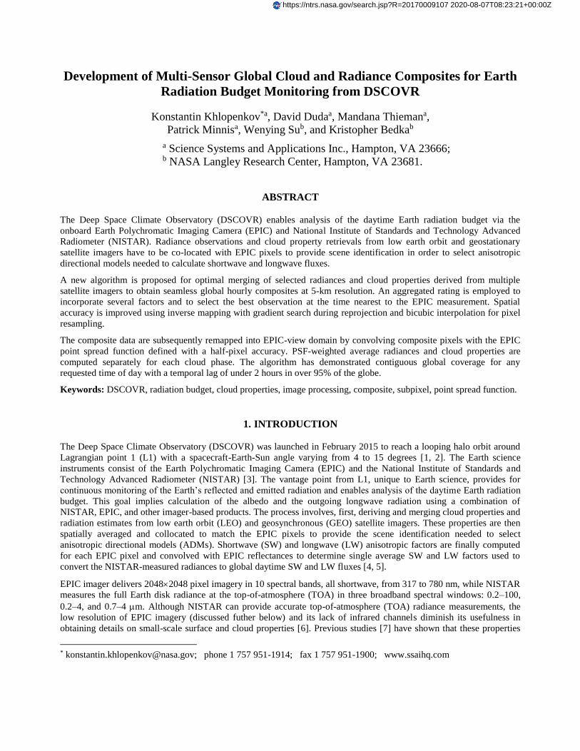
parameters is shown in Table 1. There are a few limitations here that are worth mentioning. First, the Near-Infrared

(NIR) channel is absent on GEO imagers and so reflectance in the 0.86 m band is flagged as a missing value for

composite pixels that originate from GEO satellites. Similarly, the 6.7 m water vapor band is absent for AVHRR pixels.

On GOES-12, -13, -14, and -15, the split-window brightness temperature (BT) is measured in the 13.5 m band instead

of 12 m. For this reason, BT in 12.0 m is also flagged as a missing value for composite pixels originating from those

four satellites. The surface type information is retrieved from the International Geosphere-Biosphere Programme (IGBP)

map [19], with the addition of snow and ice flags taken from the NOAA daily snow and ice cover maps at 1/6 deg spatial

Table 1. List of parameters included in global composite.

Parameter AVHRR MODIS GEOs

1 Latitude

2 Longitude

3 Solar Zenith Angle

4 View Zenith Angle

5 Relative Azimuth Angle

6 Reflectance in 0.63um 0.63 um 0.63 um 0.65 um

7 Reflectance in 0.86um 0.83 um 0.83 um —

8 BT in 3.75um 3.75 um 3.75 um 3.9 um

9 BT in 6.75um — 6.70 um 6.8 um

10 BT in 10.8um 10.8 um 10.8 um 10.8 um

11 BT in 12.0um 12.0 um 11.9 um 12/13.5

12 SW Broadband Albedo

13 LW Broadband Flux

14 Cloud Phase

15 Cloud Optical Depth

16 Cloud Effective Particle Size

17 Cloud Effective Height

18 Cloud Top Height

19 Cloud Effective Temperature

20 Cloud Effective Pressure

21 Skin Temperature (retrieved)

23 Surface Type

24 Time relative to EPIC

25 Satellite ID

Global

Composite

± 3.5 hours maximum

from IGBP + snow/ice flags

Figure 1. Global composite map of the brightness temperature in channel 10.8 m generated for Sep-15-2015

13:23UTC. The continuous coverage leaves no gaps and apparent disruptions in the temperature field.

resolution. The time relative to EPIC observation is the t from Equation (1) but converted to seconds and stored as a

signed integer number. Satellite ID is an integer number unique for each satellite which is designed to indicate the

origination of a given composite pixel.

A typical result of the compositing algorithm is presented in Figure 1, which shows an example of the map of brightness

temperature in channel 10.8 m composited for Sep-15-2015 13:23UTC. The composite image presents a continuous

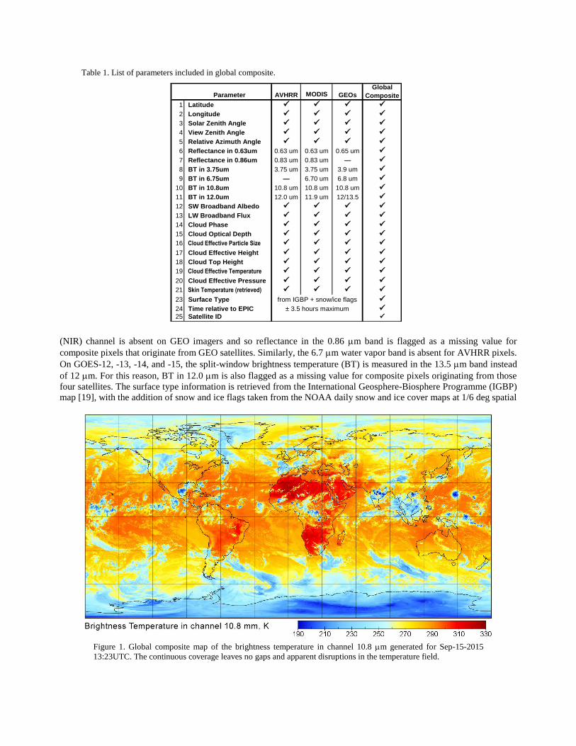
coverage with no gaps and no artificial breaks or disruptions in the temperature data. A corresponding map of satellite

ID is shown in Figure 2, which represents typical spatial coverage from different satellites. Most of the equatorial

regions are covered by GEO satellites, while the polar regions are represented by Terra and Aqua, because MODIS was

initially given a higher Fresolution factor than AVHRR. Similarly, the MET-7 data were assigned a lower Fresolution factor

in order to correct for their lower quality, and therefore the MET-7 coverage automatically shrinks and is more likely to

Figure 2. A map of satellite coverage in a global composite generated for Sep-15-2015 13:23UTC.

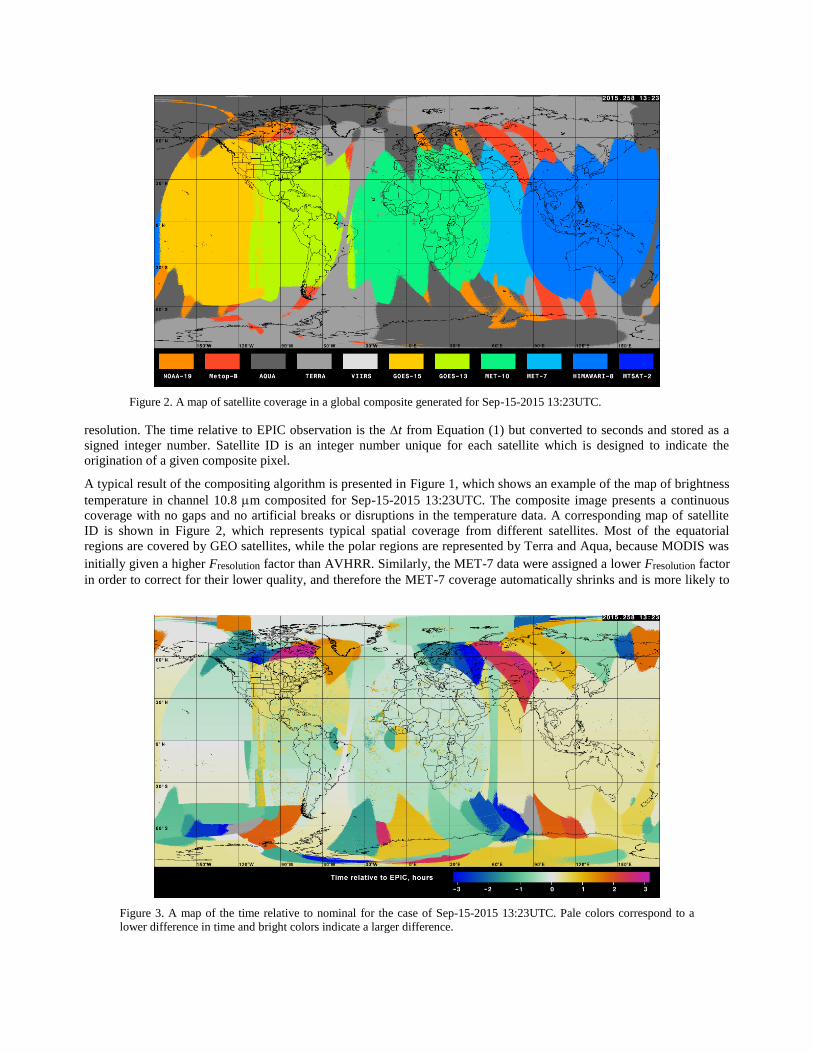
Figure 3. A map of the time relative to nominal for the case of Sep-15-2015 13:23UTC. Pale colors correspond to a

lower difference in time and bright colors indicate a larger difference.

be replaced by the adjacent MET-10 and Himawari-8 observations. A map of the time t relative to nominal (i.e. EPIC

observation) for the same case of Sep-15-2015 13:23UTC is presented in Figure 3. One can see that most of the regions

corresponding to GEO satellites (between around 50S and 50N) have a very low time difference, in the range of 30

minutes, with the exception of a small circular region on the Equator around 10W where the sun glint contamination

was replaced by prior or subsequent MET-10 observations (which occur every hour). Similar replacements may occur

when retrieved cloud phase has a low confidence. The polar regions are also covered very well by the polar orbiters

capable of observing a particular polar region nearly every overpass, which helps to decrease the t to less than an hour.

The mid-latitude regions present most of the problem: they are out of reach for GEO satellites and are observed only

twice a day by the polar orbiters. Still, most of the observations in the mid-latitudes fall within the t range of 3 hours.

This temporal lag can be reduced even further by imposing a steeper drop of the rating R as a dependence on the time

difference. This can be achieved by a lower characteristic time in Equation (1), which will automatically discard

observations with a larger time difference in favor of other alternatives, mostly those with higher VZA. This tradeoff can

be assessed by introducing an effective pixel resolution, which is obtained by adjusting the nominal pixel resolution

(specific to each satellite) to the increased pixel-to-satellite distance and the larger viewing zenith angle. Frequency

statistics of this effective resolution over the whole Earth area is demonstrated by the histogram in Figure 4A. This

distribution was obtained as the average of 22 composites produced for every EPIC observation during the same day of

Sep-15-2015. The frequency was corrected for the pixel area reduction towards the Poles and was computed as a

percentage of the total Earth surface. It is seen that most of the observations originated from MODIS and AVHRR fall in

the range of 3–6 km/pix (the nominal resolution of the CERES product based on MODIS data is 2 lines by 4 pixels,

which is taken as 3 km/pix average), while those from GEOs occupy the range of resolution from 8 km/pix to 20 km/pix

and greater. The colored curves in the figure show the percentiles of the effective resolution, which have been calculated

in three different test scenarios with the characteristic time of 4, 5, and 6 hours. Overall, 90% of the composite’s

coverage is presented by observation at 15 km/pix or better, and 95% of at least 17 km/pix.

Similar frequency distribution was obtained for the absolute time difference and is shown in Figure 4B. One can see that

most of the observations fall within about 40 minutes of the nominal composite time, which is typical of GEO satellites,

which can deliver the full disk data every hour. Looking at the percentiles, if the range of 2 hours time difference is

considered acceptable, then this requirement is met in ~94% of cases if is set to 4 hours, in ~96% of cases for =5, and

it reaches ~98% for =6 hours. Overall, 95% accuracy is considered sufficient, and so it was decided that the character-

istic time be set to 5 hours in order to limit the time difference to 2 hours in about 96% of the composite coverage.

As an inherent result of the merging process, the obtained composite may reveal uneven boundaries between data that

originate from two different satellites (see Figure 5A). These abrupt transitions are mostly due to the changing cloud

0 5 10 15 20 25

0

5

10

15

20

Pe

rce

ntile

, %

Frequency

Fre

qu

en

cy,

%

Effective pixel resolution, km/pix

80

85

90

95

100

Percentile

A.

0 1 2 3 4

0

5

10

15

20

Pe

rce

ntile

, %

Fre

qu

en

cy,

%

Absolute time difference relative to nominal, hours

Frequency

80

85

90

95

100

B.

Percentile

Figure 4. Frequency distribution of the effective pixel resolution (A) for characteristic time =5 hours. Overlaid on the

same figure are percentiles of the effective pixel resolution calculated for =4 hours (blue curve), =5 hours (black), and

=6 hours (red). Chart B shows distribution of the absolute time difference and its corresponding percentiles calculated for

the same three cases of .

coverage but can also be attributed to BRDF (bidirectional reflectance distribution function) effects. When analyzing

subsets for any kind of regional statistics, these transitions may cause unwanted random errors and biases. The pixel data

cannot, however, be blended or otherwise interpolated because it inherits all of the attributes of a particular satellite

observation, such the viewing geometry, derived cloud phase, dominant surface type, and others. This contradiction can

be resolved by introducing a certain amount of randomness when comparing the rating R and choosing between any two

satellite data (see Figure 6). When two satellite ratings R1 and R2 are very close to each other, it is not quite justified to

switch suddenly from one to the other. Instead, it is more rational to implement a gradual transition in terms of in-

creasing probability, from 0 to 1, that the second satellite source is selected. This can be realized by scaling the R2 with a

random factor that ranges within 5%, so that the following condition has to be satisfied for the rating R2 to be selected:

)1(21 rRR (5)

A. B.

Figure 5. A zoomed region of the composite brightness temperature reveals an uneven boundary between data from

different satellites (A). The same region where cumulative probability distribution was used to mix the pixel data,

which yields a smooth transition (B).

Pro

babili

ty

Sat2

Ra

tin

g,

a.u

.

Pixel position, a.u.

Sat1

Sat2 + 5%

Sat2 - 5%

0.0

1.0

randomized

Sat2 rating

Figure 6. Transition between two satellite ratings is made smoother by adding a random variable changing from –5% to

+5%. The transition occurs between the two vertical grid lines. The solid curve below is the cumulative distribution

function showing the probability that Sat2 rating is selected.

where r is a random number in the range of –0.05 to +0.05. When R1 is different from R2 by more than 5% (outside the

vertical grid lines in Figure 6) then the normal comparison is carried out. If the random number r is a normally

distributed variable, then the probability of satisfying condition (5) is described by the cumulative distribution function

shown in the lower part of the figure. The only problem is in the practical implementation. It is not easy to program a

normally distributed variable and it is even harder to efficiently calculate the cumulative distribution function for ~32

million pixels. Most programming interfaces provide a uniformly distributed random variable, but converting it to a

normally distributed number involves two logarithms, two square roots, and two trigonometric functions, severely

impairing the computational performance. This problem can resolved by using the following transformation:

)σtan(

)σtan()(

uuTn (6)

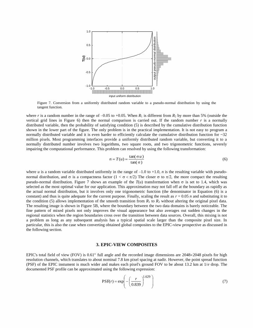
where u is a random variable distributed uniformly in the range of –1.0 to +1.0, n is the resulting variable with pseudo-

normal distribution, and is a compactness factor (1 < ) The closer to the more compact the resulting

pseudo-normal distribution. Figure 7 shows an example of the T(u) transformation when is set to 1.4, which was

selected as the most optimal value for our application. This approximation may not fall off at the boundary as rapidly as

the actual normal distribution, but it involves only one trigonometric function (the denominator in Equation (6) is a

constant) and thus is quite adequate for the current purpose. Finally, scaling the result as r = 0.05 n and substituting it to

the condition (5) allows implementation of the smooth transition from R1 to R2 without altering the original pixel data.

The resulting image is shown in Figure 5B, where the boundary between the two data domains is barely noticeable. The

fine pattern of mixed pixels not only improves the visual appearance but also averages out sudden changes in the

regional statistics when the region boundaries cross over the transition between data sources. Overall, this mixing is not

a problem as long as any subsequent analysis has a typical spatial scale larger than the composite pixel size. In

particular, this is also the case when converting obtained global composites to the EPIC-view prospective as discussed in

the following section.

3. EPIC-VIEW COMPOSITES

EPIC's total field of view (FOV) is 0.61 full angle and the recorded image dimensions are 20482048 pixels for high

resolution channels, which translates to about nominal 7.8 km pixel spacing at nadir. However, the point spread function

(PSF) of the EPIC instument is much wider and makes each pixel's ground FOV to be about 13.2 km at 1/e drop. The

documented PSF profile can be approximated using the following expression:

629.1

839.0exp)(PSF

rr (7)

-1.0 -0.5 0.0 0.5 1.0-1.0

-0.5

0.0

0.5

1.0

F1

T(u

)

outp

ut

pseu

do

-no

rma

l d

istr

ibutio

n

input uniform distribution

Figure 7. Conversion from a uniformly distributed random variable to a pseudo-normal distribution by using the

tangent function.

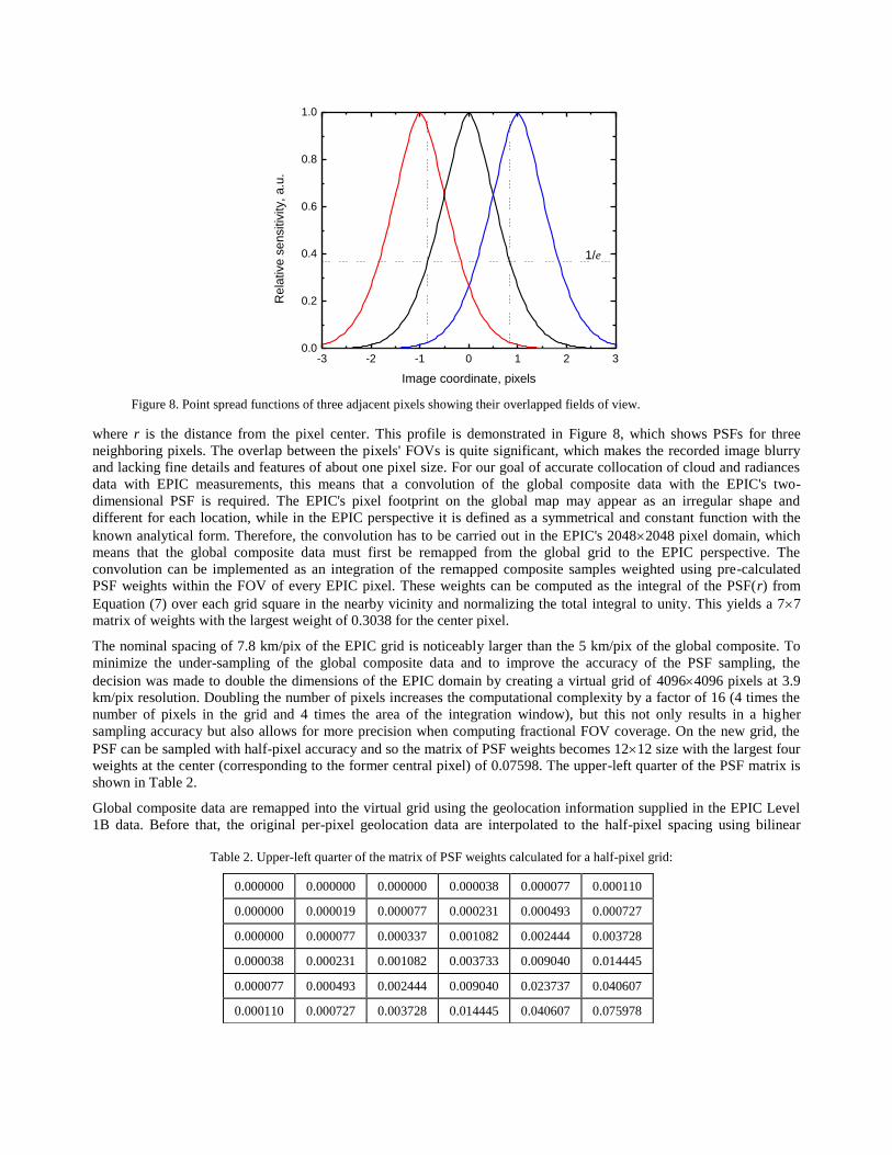
where r is the distance from the pixel center. This profile is demonstrated in Figure 8, which shows PSFs for three

neighboring pixels. The overlap between the pixels' FOVs is quite significant, which makes the recorded image blurry

and lacking fine details and features of about one pixel size. For our goal of accurate collocation of cloud and radiances

data with EPIC measurements, this means that a convolution of the global composite data with the EPIC's two-

dimensional PSF is required. The EPIC's pixel footprint on the global map may appear as an irregular shape and

different for each location, while in the EPIC perspective it is defined as a symmetrical and constant function with the

known analytical form. Therefore, the convolution has to be carried out in the EPIC's 20482048 pixel domain, which

means that the global composite data must first be remapped from the global grid to the EPIC perspective. The

convolution can be implemented as an integration of the remapped composite samples weighted using pre-calculated

PSF weights within the FOV of every EPIC pixel. These weights can be computed as the integral of the PSF(r) from

Equation (7) over each grid square in the nearby vicinity and normalizing the total integral to unity. This yields a 77

matrix of weights with the largest weight of 0.3038 for the center pixel.

The nominal spacing of 7.8 km/pix of the EPIC grid is noticeably larger than the 5 km/pix of the global composite. To

minimize the under-sampling of the global composite data and to improve the accuracy of the PSF sampling, the

decision was made to double the dimensions of the EPIC domain by creating a virtual grid of 40964096 pixels at 3.9

km/pix resolution. Doubling the number of pixels increases the computational complexity by a factor of 16 (4 times the

number of pixels in the grid and 4 times the area of the integration window), but this not only results in a higher

sampling accuracy but also allows for more precision when computing fractional FOV coverage. On the new grid, the

PSF can be sampled with half-pixel accuracy and so the matrix of PSF weights becomes 1212 size with the largest four

weights at the center (corresponding to the former central pixel) of 0.07598. The upper-left quarter of the PSF matrix is

shown in Table 2.

Global composite data are remapped into the virtual grid using the geolocation information supplied in the EPIC Level

1B data. Before that, the original per-pixel geolocation data are interpolated to the half-pixel spacing using bilinear

-3 -2 -1 0 1 2 30.0

0.2

0.4

0.6

0.8

1.0

Re

lative

se

nsitiv

ity,

a.u

.

Image coordinate, pixels

1/e

Figure 8. Point spread functions of three adjacent pixels showing their overlapped fields of view.

Table 2. Upper-left quarter of the matrix of PSF weights calculated for a half-pixel grid:

0.000000 0.000000 0.000000 0.000038 0.000077 0.000110

0.000000 0.000019 0.000077 0.000231 0.000493 0.000727

0.000000 0.000077 0.000337 0.001082 0.002444 0.003728

0.000038 0.000231 0.001082 0.003733 0.009040 0.014445

0.000077 0.000493 0.002444 0.009040 0.023737 0.040607

0.000110 0.000727 0.003728 0.014445 0.040607 0.075978

interpolation, which is sufficient here because the latitude and longitude present slow changing continuous fields

(provided that the transition at 180 longitude is unwrapped properly). These fields may change rapidly at the edge of

the EPIC-viewable Earth disk, but it was found that samples with EPIC's VZA over 87–89 have to be discarded anyway

due to apparent geolocation errors at the disk edge. The exact VZA cut-off threshold is determined individually for each

case by analyzing the smoothness of the latitude and longitude fields near the Earth disk edge.

Once the latitude and longitude are defined on the virtual grid, the composite samples are remapped by means of the

same inverse mapping but without the gradient search, which is not needed this time as the global latitude and longitude

space is equal-angle and linear. The process of remapping and convolution can be summarized in 5 steps:

1) Convert the global composite data (where applicable);

2) Remap to the virtual grid with bilinear interpolation;

3) Mask the remapped data by the cloud phase flag;

4) Convolve each of the masked subsets with the PSF weights to obtain the weighted average sample;

5) Convert the data back to the original format if needed.

The conversion is needed for angle (cosine is applied) and temperature (converted to radiance units) variables to ensure

that the subsequent averaging is correct. Also, the cloud optical depth (COD) is converted by applying the logarithm and

the obtained log(COD) is then processed as an additional variable. Other variables are converted from scaled integer

format (stored in the global composite) to floating point numbers. In Step 2, higher order interpolation is not needed

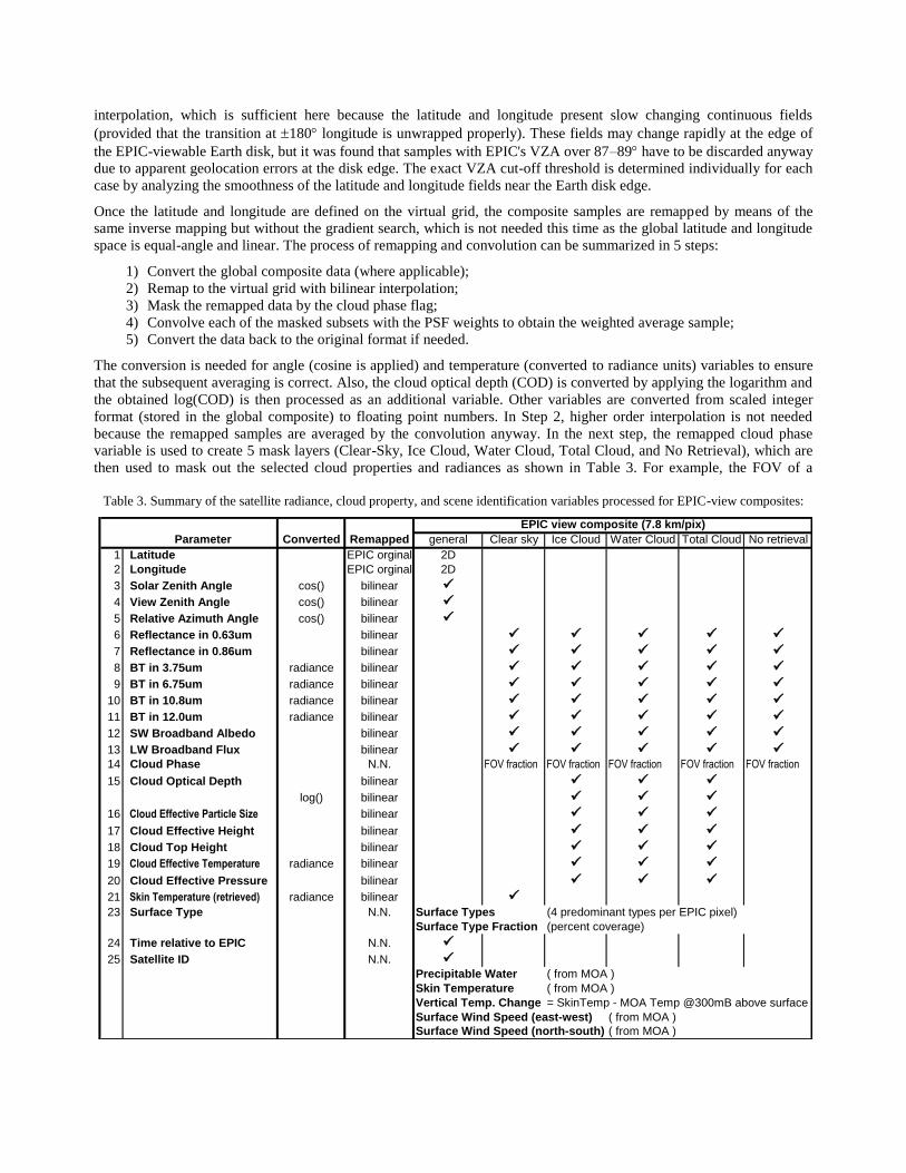
because the remapped samples are averaged by the convolution anyway. In the next step, the remapped cloud phase

variable is used to create 5 mask layers (Clear-Sky, Ice Cloud, Water Cloud, Total Cloud, and No Retrieval), which are

then used to mask out the selected cloud properties and radiances as shown in Table 3. For example, the FOV of a

Table 3. Summary of the satellite radiance, cloud property, and scene identification variables processed for EPIC-view composites:

Parameter Converted Remapped general Clear sky Ice Cloud Water Cloud Total Cloud No retrieval

1 Latitude EPIC orginal 2D

2 Longitude EPIC orginal 2D

3 Solar Zenith Angle cos() bilinear

4 View Zenith Angle cos() bilinear

5 Relative Azimuth Angle cos() bilinear

6 Reflectance in 0.63um bilinear

7 Reflectance in 0.86um bilinear

8 BT in 3.75um radiance bilinear

9 BT in 6.75um radiance bilinear

10 BT in 10.8um radiance bilinear

11 BT in 12.0um radiance bilinear

12 SW Broadband Albedo bilinear

13 LW Broadband Flux bilinear

14 Cloud Phase N.N. FOV fraction FOV fraction FOV fraction FOV fraction FOV fraction

15 Cloud Optical Depth bilinear

log() bilinear

16 Cloud Effective Particle Size bilinear

17 Cloud Effective Height bilinear

18 Cloud Top Height bilinear

19 Cloud Effective Temperature radiance bilinear

20 Cloud Effective Pressure bilinear

21 Skin Temperature (retrieved) radiance bilinear

23 Surface Type N.N. Surface Types (4 predominant types per EPIC pixel)

Surface Type Fraction (percent coverage)

24 Time relative to EPIC N.N.

25 Satellite ID N.N.

Precipitable Water

Skin Temperature

Vertical Temp. Change = SkinTemp - MOA Temp @300mB above surface

Surface Wind Speed (east-west) ( from MOA )

Surface Wind Speed (north-south) ( from MOA )

( from MOA )

EPIC view composite (7.8 km/pix)

( from MOA )

particular EPIC pixel may cover BT data having three different cloud phases. Then those BT data are screened out by

each mask in turn, weighted by the PSF matrix, and summed together to yield three different BT samples (one per

mask), which are then stored in three data subgroups (see the right side of the Table 3). The actual FOV fractions (sums

of the PSF weights screened out by the same masks), which describe the percent ratio of a particular cloud phase in a

given FOV, are also calculated and stored accordingly. A similar routine is carried out for the Surface Type variable.

The fractional coverage for each surface type is calculated as a sum of the corresponding PSF weights. Then the four

most dominant types for that FOV are selected and stored for the same EPIC pixel together with their four values of

percent coverage (called Surface Type Fraction). Additionally, the following variables are added to the EPIC composite:

Column Precipitable Water, Skin Temperature, Vertical Temperature Change (calculated as the difference between the

Skin Temperature and the temperature at 300 mBar below the surface pressure), and the Surface Wind speed vector

components. These variables are retrieved from the CERES archival product Meteorological, Ozone, and Aerosol Data

(MOA) [20], which includes hourly maps of several meteorological variables at 1 spatial resolution.

4. DISCUSSION AND CONCLUSION

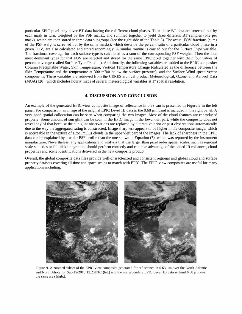
An example of the generated EPIC-view composite image of reflectance in 0.63 m is presented in Figure 9 in the left

panel. For comparison, an image of the original EPIC Level 1B data in the 0.68 m band is included in the right panel. A

very good spatial collocation can be seen when comparing the two images. Most of the cloud features are reproduced

properly. Some amount of sun glint can be seen in the EPIC image in the lower-left part, while the composite does not

reveal any of that because the sun glint observations are replaced by alternative prior or past observations automatically

due to the way the aggregated rating is constructed. Image sharpness appears to be higher in the composite image, which

is noticeable in the texture of altocumulus clouds in the upper-left part of the images. The lack of sharpness in the EPIC

data can be explained by a wider PSF profile than the one shown in Equation (7), which was reported by the instrument

manufacturer. Nevertheless, any applications and analysis that use larger than pixel order spatial scales, such as regional

scale statistics or full disk integration, should perform correctly and can take advantage of the added IR radiances, cloud

properties and scene identifications delivered in the new composite product.

Overall, the global composite data files provide well-characterized and consistent regional and global cloud and surface

property datasets covering all time and space scales to match with EPIC. The EPIC-view composites are useful for many

applications including:

Figure 9. A zoomed subset of the EPIC-view composite generated for reflectance in 0.63 m over the North Atlantic

and North Africa for Sep-15-2015 13:23UTC (left) and the corresponding EPIC Level 1B data in band 0.68 m over

the same area (right).

Inter-calibration of non-UV EPIC channels;

Provide high-resolution independent scene identification for each EPIC pixel;

Convolve with EPIC radiances and CERES ADMs to compute daytime fluxes from NISTAR;

Serve as a comparison source for EPIC cloud retrievals;

Provide cloud mask for other retrievals based on EPIC radiances.

The global composite development presents a high scientific value on its own without the EPIC-related applications as it

provides both a reliable method and a versatile product obtained by aggregating the best modern and historic satellite

data. The key to this approach is data quality filtering, intercalibration, advanced remapping with merging, and rigorous

scientific evaluation of the cloud and radiation data products from several satellite observing systems. High spatial

accuracy is achieved by using the inverse mapping with the gradient search during reprojection and multi-sample

interpolation for pixel resampling. Spatial variability and continuity of the global composite data have been analyzed to

assess the performance of the merging criteria. A smoother transition in the merged output is achieved by enhancing the

selection decision with the cumulative probability function of the normal distribution so that abrupt changes in the visual

appearance of the composite data are avoided. The described algorithm has demonstrated seamless global coverage for

any requested time of day with a temporal lag of under 2 hours in over 95% of the globe. The global satellite data

composites provide an independent source of radiance measurements, cloud properties, and scene identification

information necessary to construct ADMs that are used to determine the daytime Earth radiation budget. The composite

dataset worth of more than 1.5 years of data is now being generated, tested, and documented. The product will soon

become available through NASA Langley Atmospheric Sciences Data Center (ASDC).

5. REFERENCES

[1] Burt, J., Smith, B., “Deep Space Climate Observatory: The DSCOVR mission,” 2012 IEEE Aerospace Conference,

IEEE, doi: 10.1109/AERO.2012.6187025 (2012).

[2] NOAA Space Weather Prediction Center, “Deep Space Climate Observatory (DSCOVR). NOAA National Centers

for Environmental Information,” Dataset, doi:10.7289/V51Z42F7 (2016).

[3] Herman, J. R., Marshak, A. and Szabo, A., “DSCOVR/EPIC Images and Science: A New Way to View the Entire

Sunlit Earth From A Sun-Earth Lagrange-1 Orbit,” Proc. of AGU Fall Meeting Abstracts, 2015AGUFM.A21I..01H

(2015).

[4] Su, W., Corbett, J., Eitzen, Z. and Liang, L., “Next-generation angular distribution models for top-of-atmosphere

radiative flux calculation from CERES instruments: methodology,” Atmos. Meas. Tech., 8, 611–632,

doi:10.5194/amt-8-611-2015 (2015).

[5] Su, W., Corbett, J., Eitzen, Z. and Liang, L., “Next-generation angular distribution models for top-of-atmosphere

radiative flux calculation from CERES instruments: validation,” Atmos. Meas. Tech., 8, 3297–3313,

doi:10.5194/amt-8-3297-2015 (2015).

[6] Meyer, K., Yang, Y. and Platnick, S., “Uncertainties in cloud phase and optical thickness retrievals from the Earth

Polychromatic Imaging Camera (EPIC),” Atmos. Meas. Tech., 9, 1785–1797, doi:10.5194/amt-9-1785-2016

(2016).

[7] Loeb, N. G., Parol, F., Buriez, J.-C. and Vanbauce, C., “Top-of-atmosphere albedo estimation from angular

distribution models using scene identification from satellite cloud property retrievals,” J. Climate, 13, 1269–1285,

doi:10.1175/1520-0442(2000)013<1269:TOAAEF>2.0.CO;2 (2000).

[8] Wielicki, B. A., Barkstrom, B. R., Harrison, E. F., Lee III, R. B., Smith, G. L. and Cooper, J. E., “Clouds and the

Earth's Radiant Energy System (CERES): An Earth Observing System Experiment,” Bull. Amer. Meteor. Soc., 77,

853–868, doi:10.1175/1520-0477(1996)077<0853:CATERE>2.0.CO;2 (1996).

[9] Doelling, D. R., Sun, M., Nguyen, L. T., Nordeen, M. L., Haney, C. O., Keyes, D. F. and Mlynczak, P. E.,

“Advances in Geostationary-Derived Longwave Fluxes for the CERES Synoptic (SYN1deg) Product,” J. Atmos.

Oceanic Technol., 33(3), 503–521, doi:10.1175/JTECH-D-15-0147.1 (2016).

[10] Lazzara, M. A., Benson, J. M., Fox, R. J., Laitsch, D. J., Rueden, J. P., Satnek, D. A., Wade, D. M., Whittaker, T.

M., Young, J. T., “The Man computer Interactive Data Access System: 25 years of Interactive Processing,” Bull.

Amer. Meteor. Soc., 80(2), 271, doi:10.1175/1520-0477(1999)080<0271:TMCIDA>2.0.CO;2 (1999).

[11] Minnis, P., Sun-Mack, S., Young, D. F., Heck, P. W., Garber, D. P., Chen, Y., Spangenberg, D. A., Arduini, R. F.,

Trepte, Q. Z., Smith, W. L. Jr., Ayers, J. K., Gibson, S. C., Miller, W. F., Chakrapani, V., Takano, Y., Liou, K.-N.,

Xie, Y. and Yang, P., “CERES Edition-2 cloud property retrievals using TRMM VIRS and Terra and Aqua

MODIS data, Part I: Algorithms,” IEEE Trans. Geosci. Remote Sens., 49, 4374–4400, doi:

10.1109/TGRS.2011.2144601 (2011).

[12] Minnis, P., Sun-Mack, S., Chen, Y., Khaiyer, M. M., Yi, Y., Ayers, J. K., Brown, R. R., Dong, X., Gibson, S. C.,

Heck, P. W., Lin, B., Nordeen, M. L., Nguyen, L., Palikonda, R., Smith, W. L. Jr., Spangenberg, D. A., Trepte, Q.

Z., and Xi, B., “CERES Edition-2 cloud property retrievals using TRMM VIRS and Terra and Aqua MODIS data,

Part II: Examples of average results and comparisons with other data,” IEEE Trans. Geosci. Remote Sens., 49,

4401–4430, doi: 10.1109/TGRS.2011.2144602 (2011).

[13] Minnis, P., Bedka, K., Trepte, Q. Z., Yost, C. R., Bedka, S. T., Scarino, B., Khlopenkov, K. V., and Khaiyer, M.

M., “A consistent long-term cloud and clear-sky radiation property dataset from the Advanced Very High

Resolution Radiometer (AVHRR). Climate Algorithm Theoretical Basis Document (C-ATBD),” CDRP-ATBD-

0826 Rev 1–NASA, NOAA CDR Program, 159 pp., DOI:10.789/V5HT2M8T, <http://ww.ncdc.noaa.gov/cdr/

atmospheric/avhrr-cloud-properties-nasa> (2016).

[14] Khlopenkov, K. V. and Trishchenko, A. P., “Achieving Subpixel Georeferencing Accuracy in the Canadian

AVHRR Processing System,” IEEE Trans. Geosci. Remote Sens., 48(4), 2150–2161

doi:10.1109/TGRS.2009.2034974 (2010).

[15] Weinreb, M. P, Xie, R., Lienesch, J. H., and Crosby, D. S., “Destriping GOES Images by Matching Empirical

Distribution Functions,” Remote Sens. Environ., 29, 185–195, doi:10.1016/0034-4257(89)90026-6 (1989).

[16] Khlopenkov, K. V. and Doelling, D. R., “Development of Image Processing Method to Detect Noise in

Geostationary Imagery,” Proc. SPIE 10004, Image and Signal Processing for Remote Sensing XXII, 100041S,

doi: 10.1117/12.2241544 (2016).

[17] Khlopenkov, K. V., Trishchenko, A. P., “Implementation and Evaluation of Concurrent Gradient Search Method

for Reprojection of MODIS Level 1B Imagery,” IEEE Trans. Geosci. Remote Sens., 46(7), 2016–2027, doi:

10.1109/TGRS.2008.916633 (2008).

[18] Duchon, C. E., “Lanczos Filtering in One and Two Dimensions,” J. Appl. Meteor., 18, 1016–1022,

doi:10.1175/1520-0450(1979)018<1016:LFIOAT>2.0.CO;2 (1979).

[19] International Geosphere Biosphere Programme, Improved Global Data for Land Applications, edited by J. R. G.

Townshend. IGBP Global Change Report No. 20, International Geosphere–Biosphere Programme, Stockholm,

Sweden, 87 pp. (1992).

[20] Caldwell, T. E., Coleman, L. H., Cooper, D. L., Escuadra, J., Fan, A., Franklin, C. B., Halvorson, J. A., Hess, P. C.,

Kizer, E. A., McKoy, N. C., Murray, T. D., Nguyen, L. T., Nolan, S. K., Raju, R. J., Robbins, L., Stassi, J. C., Sun-

Mack, S., Tolson, C. J., Costulis, P. K., Geier, E. B., Kibler, J. F., Mitchum, M. V., “Clouds and the Earth's Radiant

Energy System (CERES), Data Management System, Data Products Catalog, Release 4, Version 16,”

<https://eosweb.larc.nasa.gov/sites/default/files/project/ceres/readme/dpc_R4V16.pdf> (February 2008)