development of novel approaches for high resolution ... · approaches for high resolution direction...
TRANSCRIPT

Development Of Novel Approaches For High Resolution Direction Of Arrival Estimation Techniques Balasubramanian, R. K. Submitted version deposited in Coventry University’s Institutional Repository Original citation: Balasubramanian, R. K. (2016) Development Of Novel Approaches For High Resolution Direction Of Arrival Estimation Techniques. Unpublished PhD Thesis. Coventry: Coventry University Copyright © and Moral Rights are retained by the author. A copy can be downloaded for personal non-commercial research or study, without prior permission or charge. This item cannot be reproduced or quoted extensively from without first obtaining permission in writing from the copyright holder(s). The content must not be changed in any way or sold commercially in any format or medium without the formal permission of the copyright holders. Some materials have been removed from this thesis due to third party copyright. Pages where material has been removed are clearly marked in the electronic version. The unabridged version of the thesis can be viewed at the Lanchester Library, Coventry University.

DEVELOPMENT OF NOVEL APPROACHES FOR HIGH RESOLUTION DIRECTION OF ARRIVAL ESTIMATION
TECHNIQUES
RAMASWAMY KARTHIKEYAN BALASUBRAMANIAN
September 2015
By
A thesis submitted in partial fulfilment of the University’s requirements for the Degree of Doctor of Philosophy

CERTIFICATE
This is to certify that the Doctoral Dissertation titled “Development
of Novel Approaches for Direction of Arrival Estimation Techniques”
is a bonafide record of the work carried out by Mr. Ramaswamy
Karthikeyan Balasubramanian in partial fulfilment of requirements
for the award of Doctor of Philosophy Degree of Coventry University
September - 2015
Dr. Govind R. Kadambi Diretor of Studies M.S.Ramaiah School of Advanced Studies, Bangalore Dr. Govind R. Kadambi Supervisor M.S.Ramaiah School of Advanced Studies, Bangalore Dr. Yuri A. Vershinin Supervisor Coventry University, U.K .

ACKNOWLEDGEMENT
The successful completion of any task would be incomplete without complementing those
who made it possible and whose guidance and encouragement ensured its success.
I thank my mother Mrs. B. Thilakavathi and my father Mr. R. Balasubramanianfor their unconditional love and support. I am forever indebted to them and very sincerely
acknowledge their forbearance during this period. Their support has steadfastly sustained
my motivation to culminate all my doctoral research work into this thesis.
I am overwhelmed at this point of time to express my sincere and heartfelt gratitude
to my supervisor Professor Govind R. Kadambi, Pro-Vice Chancellor, M S Ramaiah
University of Applied Sciences, Bangalore. His guidance and sustained motivation are the
backbone in the progress of this research. I profusely thank him for the same.
I am thankful to my supervisor Dr. Yuri A. Vershinin, Senior Lecturer, Coventry Uni-
versity, U.K. His guidance and monitoring of my research progress and thesis preparation
helps me to reach this level.
With deep sense of gratitude and indebtedness, I acknowledge the support, guidance and
encouragement rendered by, Professor S.R. Shankapal, Vice Chancellor, M S Ramaiah
University of Applied Sciences. While his advice have been a source of inspiration, his
suggestions and feedback proved to be valuable course correctors throughout the tenure of
my research work at MSRSAS.
I thank Professor M.D. Deshpande, Head, Research Department, MSRSAS, for pro-
viding necessary resources, facilities and an excellent environment conducive to research
work. His politeness and conduction of research reviews are worthy of emulation.
I take this opportunity to express my gratitude to Professor Peter White, Coventry
University, U.K. for his thought provoking suggestions and also key inputs provided during
the progress review meetings. His comments helped me a lot in understanding the purpose
of research. I am ever grateful to him for his kindness and patient listening during review
meetings.
I offer my most humble submission and thanks to ALMIGHTY GOD for his grace
and immeasurable blessings.
i
ABSTRACT
This thesis presents the development of MUSIC algorithm based novel approaches for the
estimation of Direction of Arrival (DOA) of electromagnetic sources. For the 2D-DOA estimation,
this thesis proposes orthogonally polarized linear array configuration rather than the conventionally
invoked two dimensional array. An elegant one dimensional search technique to compute 2D-DOA
estimation for a single source scenario has been proposed. To facilitate one dimensional search
for 2D-DOA estimation, a closed form relationship between the azimuth and elevation angles
of the 2D-DOA is derived using the analytical expressions of radiation patterns of Rectangular
Waveguide (RWG) and Circular Waveguide (CWG). The computation time for the proposed one
dimensional search technique is reduced by a factor of 50 and 150 for 1◦ and 0.5◦ search interval
respectively. To improve the accuracy and the resolution of 2D-DOA estimation in case of closely
spaced sources, this thesis proposes novel array configurations such as orthogonally polarized
planar array, orthogonally mounted linear array and orthogonally polarized linear array. Through
numerous simulation studies, a relative performance comparison of 2D-DOA estimation realized
through various proposed novel array configurations has been carried out to highlight the accu-
racy and resolution under wide range of SNR conditions. The thesis presents a discussion on
the analysis of effect of spatial de correlation in lieu of the employed orthogonally polarized ele-
ments in the array configuration on the improved accuracy and resolution of the 2D-DOA estimation.
This thesis also deals with the utility of the proposed orthogonally polarized array configura-
tions for tracking of 2D-DOA angles of non-stationary signal sources. The weighting factor and
forgetting factor approaches for smoothing the time-varying covariance matrix of the non-stationary
sources are studied. The simulation studies on 2D-DOA tracking by invoking proposed array
configurations along with the proposed smoothing techniques prove that orthogonal polarized array
configuration track the DOA source angle with minimum estimation errors. The thesis proposes
the replacement of computationally intensive numerical schemes in Multiple Signal Classification
(MUSIC) algorithm such as eigen decomposition and singular value decomposition with the sub-
space tracking techniques such as Bi-Iterative Singular Value Decomposition (Bi-SVD) algorithm.
Invoking the concept of sub-band processing, the thesis addresses the validity of the extension of
the presented 2D-DOA estimation analysis to wide band signal. A two subband filter approach is
proposed for the estimation 2D-DOA of single and two wideband sources. The simulation study of
the two subband filter approach along with the orthogonal polarized array configurations confirms
the better estimation accuracy as well as the lesser computation time.
ii

CONTENTS
Acknowledgement i
Abstract ii
Contents iii
List of Tables xi
List of Figures xii
Nomenclature xxiv
List of Abbreviations xxvi
1 Introduction 11.1 Introduction to DOA Estimation . . . . . . . . . . . . . . . . . . . . . . 1
1.2 Applications of DOA Estimation . . . . . . . . . . . . . . . . . . . . . . 2
1.3 DOA Estimation Algorithms . . . . . . . . . . . . . . . . . . . . . . . . 4
1.4 Motivation of the Research . . . . . . . . . . . . . . . . . . . . . . . . . 8
1.5 Objectives of the Thesis . . . . . . . . . . . . . . . . . . . . . . . . . . . 9
1.6 Organization of the Thesis . . . . . . . . . . . . . . . . . . . . . . . . . 10
2 Review of Antenna Arrays and DOA Estimation Algorithms 122.1 Antennas . . . . . . . . . . . . . . . . . . . . . . . . . . . . . . . . . . . 12
2.1.1 Radiation Pattern . . . . . . . . . . . . . . . . . . . . . . . . . . 12
2.1.2 Antenna Polarization . . . . . . . . . . . . . . . . . . . . . . . . 14
2.1.3 Illumination of Sources . . . . . . . . . . . . . . . . . . . . . . . 16
2.2 Antenna Arrays . . . . . . . . . . . . . . . . . . . . . . . . . . . . . . . 18
2.2.1 Array Factor . . . . . . . . . . . . . . . . . . . . . . . . . . . . . 18
2.2.2 Pattern Multiplication . . . . . . . . . . . . . . . . . . . . . . . . 19
2.2.3 Array Manifold . . . . . . . . . . . . . . . . . . . . . . . . . . . 19
iii

2.2.4 Effect of Antenna Element Pattern . . . . . . . . . . . . . . . . . 20
2.3 Antenna Array Configurations . . . . . . . . . . . . . . . . . . . . . . . 21
2.3.1 One-Dimensional Array . . . . . . . . . . . . . . . . . . . . . . 22
2.3.2 Two-Dimensional Array . . . . . . . . . . . . . . . . . . . . . . 23
2.3.2.1 Uniform Planar Array . . . . . . . . . . . . . . . . . . 23
2.3.2.2 Uniform Circular Array . . . . . . . . . . . . . . . . . 23
2.3.2.3 Cross Array . . . . . . . . . . . . . . . . . . . . . . . . 24
2.3.2.4 Orthogonal Array . . . . . . . . . . . . . . . . . . . . 25
2.3.3 Three Dimensional Array . . . . . . . . . . . . . . . . . . . . . . 26
2.3.3.1 L-Shaped Arrays . . . . . . . . . . . . . . . . . . . . . 26
2.4 Review of DOA Estimation Algorithms . . . . . . . . . . . . . . . . . . 28
2.4.1 Antenna Array Signal Modelling . . . . . . . . . . . . . . . . . . 28
2.4.2 Uniform Linear Array (ULA) . . . . . . . . . . . . . . . . . . . . 29
2.4.3 Assumptions in the DOA Estimation Schemes . . . . . . . . . . . 31
2.5 Classification of DOA Estimation Algorithms . . . . . . . . . . . . . . . 32
2.5.1 Beamforming Based DOA Estimation Techniques . . . . . . . . . 32
2.5.1.1 Bartlett’s Conventional Beamformer . . . . . . . . . . . 33
2.5.1.2 Capon’s MVDR Algorithm . . . . . . . . . . . . . . . 34
2.5.2 Subspace Based Estimation Techniques . . . . . . . . . . . . . . 34
2.5.2.1 Pisarenko Harmonic Decomposition . . . . . . . . . . . 37
2.5.2.2 MUSIC Algorithm . . . . . . . . . . . . . . . . . . . . 37
2.5.2.3 Root MUSIC Algorithm . . . . . . . . . . . . . . . . . 38
2.5.2.4 ESPRIT Algorithm . . . . . . . . . . . . . . . . . . . . 38
2.5.2.5 Other Methods . . . . . . . . . . . . . . . . . . . . . . 42
2.6 Antenna Elements and Array Configuration for DOA Estimation . . . . . 43
2.7 DOA Tracking of Non Stationary Signal Sources . . . . . . . . . . . . . 47
2.7.1 Singular Value Decomposition (SVD) . . . . . . . . . . . . . . . 48
2.7.2 Subspace Tracking Algorithms . . . . . . . . . . . . . . . . . . . 49
2.8 DOA Estimation of Wideband Signals . . . . . . . . . . . . . . . . . . . 50
2.8.1 Approximation of Narrow Band Signal . . . . . . . . . . . . . . . 51
2.8.2 Wideband Signal Model for Linear Array . . . . . . . . . . . . . 52
2.8.3 DOA Estimation of Wideband Sources . . . . . . . . . . . . . . . 54
2.8.4 Incoherent Method . . . . . . . . . . . . . . . . . . . . . . . . . 55
2.8.5 Coherent Signal Subspace Method . . . . . . . . . . . . . . . . . 56
iv
2.9 Summary . . . . . . . . . . . . . . . . . . . . . . . . . . . . . . . . . . 57
3 Formulation and Analysis of a Closed Form Solution for Two DimensionalDOA Estimation 593.1 Introduction . . . . . . . . . . . . . . . . . . . . . . . . . . . . . . . . . 59
3.2 Review of 2D-DOA Estimation Techniques . . . . . . . . . . . . . . . . 59
3.3 Open Ended Waveguide as an Antenna Element . . . . . . . . . . . . . . 61
3.3.1 Proposed Orthogonally Polarized Linear Array Configuration . . . 62
3.4 Signal Modelling with RWG Array Elements . . . . . . . . . . . . . . . 65
3.5 2D-DOA Estimation Using Closed Form Solutions . . . . . . . . . . . . 66
3.5.1 Derivation to Relate Azimuth and Elevation DOA Angles with RWG 67
3.5.2 Derivation to Relate Azimuth and Elevation DOA Angles with CWG 69
3.5.3 Reduction of Search Dimension of 2D DOA Estimation using
Closed Form Solution . . . . . . . . . . . . . . . . . . . . . . . . 70
3.5.4 Simulation Analysis of Proposed One Dimensional Search Tech-
nique for 2D-DOA . . . . . . . . . . . . . . . . . . . . . . . . . 72
3.5.5 RMSE Analysis . . . . . . . . . . . . . . . . . . . . . . . . . . . 74
3.6 Summary . . . . . . . . . . . . . . . . . . . . . . . . . . . . . . . . . . 76
4 Two Dimensional DOA Estimation using Dual Polarized Array for Singleand Multiple Sources 774.1 Introduction . . . . . . . . . . . . . . . . . . . . . . . . . . . . . . . . . 77
4.1.1 Antenna Configurations for 2D-DOA Estimation . . . . . . . . . 77
4.2 Antenna Element Radiation Pattern in DOA . . . . . . . . . . . . . . . . 78
4.3 Signal Model . . . . . . . . . . . . . . . . . . . . . . . . . . . . . . . . 78
4.4 Diversely (Dual) Polarized Antenna Array . . . . . . . . . . . . . . . . . 79
4.5 Antenna Array Configuration . . . . . . . . . . . . . . . . . . . . . . . . 80
4.5.1 Uniform Planar Array (UPA) . . . . . . . . . . . . . . . . . . . . 80
4.5.2 Orthogonally Polarized Planar Array (OPPA) . . . . . . . . . . . 81
4.5.3 Orthogonally Mounted Linear Array (OMLA) . . . . . . . . . . . 82
4.5.4 Orthogonally Polarized Linear Array (OPLA) . . . . . . . . . . . 82
4.6 Simulation Environment . . . . . . . . . . . . . . . . . . . . . . . . . . 83
4.7 Analysis of Accuracy of Estimation of 2D-DOA . . . . . . . . . . . . . . 83
4.7.1 Broadside Illumination . . . . . . . . . . . . . . . . . . . . . . . 84
v
4.7.2 End-fire Illumination . . . . . . . . . . . . . . . . . . . . . . . . 87
4.8 Discussion of Results on 2D-DOA of Single Source . . . . . . . . . . . . 90
4.9 Analysis of 2D-DOA Estimation for Two Sources . . . . . . . . . . . . . 91
4.9.1 Results of 2D-DOA of Two Sources at 20 dB SNR . . . . . . . . 91
4.9.2 Results of 2D-DOA of Two Sources at 10 dB SNR . . . . . . . . 94
4.9.3 Results of 2D-DOA of Two Sources at 0 dB SNR . . . . . . . . . 96
4.9.4 Inference from the Results of 2D-DOA of Two Sources . . . . . . 99
4.9.5 Eigenvalues based Scheme for Distinguishing Sources . . . . . . 100
4.9.6 Inference of Eigenvalues under various SNRs . . . . . . . . . . . 103
4.10 2D-DOA for Three Sources at SNR of 0 dB . . . . . . . . . . . . . . . . 104
4.10.1 Inference from the Results of 2D-DOA on Estimation of Three
Sources . . . . . . . . . . . . . . . . . . . . . . . . . . . . . . . 107
4.11 Analysis of Sharpness of Peak in 2D-DOA Estimation . . . . . . . . . . . 107
4.12 Resolution Analysis of 2D-DOA Estimation with Closely Spaced Two
Sources . . . . . . . . . . . . . . . . . . . . . . . . . . . . . . . . . . . 110
4.12.1 Analysis of 2D-DOA Estimation of Closely Spaced Two Sources
using UPA . . . . . . . . . . . . . . . . . . . . . . . . . . . . . . 110
4.12.2 Analysis of 2D-DOA of Closely Spaced Two Sources using OPPA 112
4.12.3 Analysis of 2D-DOA Estimation of Closely Spaced Two Sources
using OMLA . . . . . . . . . . . . . . . . . . . . . . . . . . . . 113
4.12.4 Analysis of 2D-DOA Estimation of Closely Spaced Two Sources
using OPLA . . . . . . . . . . . . . . . . . . . . . . . . . . . . . 115
4.13 Analysis of Effect of Inter Element Spacing on the 2D-DOA Estimation
Performance . . . . . . . . . . . . . . . . . . . . . . . . . . . . . . . . . 118
4.14 Summary . . . . . . . . . . . . . . . . . . . . . . . . . . . . . . . . . . 120
5 Two Dimensional DOA Tracking of Non-Stationary Sources using SubspaceTracking Algorithms 1215.1 Introduction . . . . . . . . . . . . . . . . . . . . . . . . . . . . . . . . . 121
5.1.1 Adaptive Eigen Decomposition Algorithms . . . . . . . . . . . . 121
5.1.2 Eigen Based DOA Tracking Algorithms . . . . . . . . . . . . . . 122
5.1.3 Bi-SVD Algorithm . . . . . . . . . . . . . . . . . . . . . . . . . 123
5.2 Modelling of Signal Sources for Tracking of 2D-DOA . . . . . . . . . . . 124
5.2.1 Modelling of Stationary Source . . . . . . . . . . . . . . . . . . . 124
vi

5.2.2 Modelling of Non-stationary Source . . . . . . . . . . . . . . . . 125
5.2.3 Covariance Matrix by Weighting Factor α . . . . . . . . . . . . . 125
5.2.4 Forgetting Factor β Method for Covariance Matrix . . . . . . . . 126
5.3 Simulation Analysis of DOA of Non-Stationary Sources . . . . . . . . . . 126
5.3.1 Tracking of DOA with MUSIC Algorithm . . . . . . . . . . . . . 126
5.4 Analysis of Weighting and Forgetting Factor in 2D-DOA Estimation and
Tracking . . . . . . . . . . . . . . . . . . . . . . . . . . . . . . . . . . . 129
5.4.1 Weighting Factor Analysis for Tracking of Estimation of 2D-DOA 129
5.4.2 Forgetting Factor Analysis for Tracking of Estimation of 2D-DOA 130
5.5 Analysis of 2D-DOA Tracking Behaviour of Single and Orthogonal Polar-
ized Arrays . . . . . . . . . . . . . . . . . . . . . . . . . . . . . . . . . 132
5.5.1 Tracking Behaviour of 2D-DOA Estimation with Single Polarized
UPA . . . . . . . . . . . . . . . . . . . . . . . . . . . . . . . . . 132
5.5.1.1 Tracking of 2D-DOA Estimation with UPA using Instan-
taneous Samples . . . . . . . . . . . . . . . . . . . . . 133
5.5.1.2 Tracking of 2D-DOA Estimation with UPA using Weight-
ing Factor . . . . . . . . . . . . . . . . . . . . . . . . . 133
5.5.1.3 Tracking of 2D-DOA Estimation with UPA using Forget-
ting Factor . . . . . . . . . . . . . . . . . . . . . . . . 134
5.5.2 Tracking Behaviour of 2D-DOA Estimation with OPPA . . . . . . 135
5.5.2.1 Tracking of 2D-DOA Estimation with OPPA using In-
stantaneous Samples . . . . . . . . . . . . . . . . . . . 136
5.5.2.2 Tracking of 2D-DOA Estimation with OPPA using Weight-
ing Factor . . . . . . . . . . . . . . . . . . . . . . . . . 137
5.5.2.3 Tracking of 2D-DOA Estimation with OPPA using For-
getting Factor . . . . . . . . . . . . . . . . . . . . . . . 138
5.5.3 Tracking Behaviour of 2D-DOA Estimation with OMLA . . . . . 139
5.5.3.1 Tracking of 2D-DOA Estimation with OMLA using In-
stantaneous Samples . . . . . . . . . . . . . . . . . . . 139
5.5.3.2 Tracking of 2D-DOA Estimation with OMLA using
Weighting Factor . . . . . . . . . . . . . . . . . . . . . 140
5.5.3.3 Tracking of 2D-DOA Estimation with OMLA using For-
getting Factor . . . . . . . . . . . . . . . . . . . . . . . 141
5.5.4 Tracking Behaviour of 2D-DOA Estimation with OPLA . . . . . 142
vii

5.5.4.1 Tracking of 2D-DOA Estimation with OPLA using In-
stantaneous Samples . . . . . . . . . . . . . . . . . . . 143
5.5.4.2 Tracking of 2D-DOA Estimation with OPLA using Weight-
ing Factor . . . . . . . . . . . . . . . . . . . . . . . . . 144
5.5.4.3 Tracking of 2D-DOA Estimation with OPLA using For-
getting Factor . . . . . . . . . . . . . . . . . . . . . . . 144
5.6 Computation Analysis of MSE versus SNR in Tracking Behaviour of
2D-DOA Estimation with Single Polarized and Orthogonal Polarized Arrays145
5.6.1 MSE Performance Analysis of Tracking Behaviour of 2D-DOA
Estimation with Instantaneous Samples . . . . . . . . . . . . . . 146
5.6.2 MSE Performance Analysis of Tracking Behaviour of 2D-DOA
Estimation with Weighting Factor . . . . . . . . . . . . . . . . . 147
5.6.3 MSE Performance Analysis of Tracking Behaviour of 2D-DOA
Estimation with Forgetting Factor . . . . . . . . . . . . . . . . . 149
5.7 Summary . . . . . . . . . . . . . . . . . . . . . . . . . . . . . . . . . . 153
6 DOA Estimation of Wideband Sources 1546.1 Introduction . . . . . . . . . . . . . . . . . . . . . . . . . . . . . . . . . 154
6.2 Sub-band Filtering Approach . . . . . . . . . . . . . . . . . . . . . . . . 155
6.3 Simulation Analysis of DOA Estimation of Wideband Sources . . . . . . 156
6.3.1 Wideband Signal Model . . . . . . . . . . . . . . . . . . . . . . 157
6.3.2 Incoherent Method for DOA Estimation of Wideband Signal . . . 157
6.4 Coherent Signal Subspace Method (CSSM) for Wideband DOA Estimation 161
6.4.1 Subband Technique for Wideband DOA Estimation . . . . . . . . 162
6.5 Comparison of DOA Estimation Techniques for Wideband Signal . . . . . 166
6.5.1 Computation Time Analysis of Wideband DOA Methods . . . . . 169
6.6 Simulation of DOA Estimation Techniques for Two Wideband Sources . . 170
6.6.1 Estimation of DOA of Two Wideband Sources θ1 = 10◦, and θ2 =
40◦ . . . . . . . . . . . . . . . . . . . . . . . . . . . . . . . . . 170
6.6.2 Estimation of DOA of Two Wideband Sources θ1 = −10◦, and
θ2 = 20◦ . . . . . . . . . . . . . . . . . . . . . . . . . . . . . . . 173
6.6.3 Estimation of DOA of Two Wideband Sources θ1 = −30◦, and
θ2 = 40◦ . . . . . . . . . . . . . . . . . . . . . . . . . . . . . . 175
viii

6.7 Simulation of 2D-DOA Estimation of Wideband Source by Using Subband
Technique . . . . . . . . . . . . . . . . . . . . . . . . . . . . . . . . . . 177
6.7.1 Wideband Signal Model for 2D-DOA . . . . . . . . . . . . . . . 177
6.7.2 2D-DOA Estimation of Wideband Source Using Conventional
Single Polarized UPA . . . . . . . . . . . . . . . . . . . . . . . . 178
6.7.3 2D-DOA Estimation of Wideband Source with OPPA . . . . . . . 180
6.7.4 2D-DOA Estimation of Wideband Source with OMLA . . . . . . 181
6.7.5 2D-DOA Estimation of Wideband Source with OPLA . . . . . . . 183
6.7.6 RMSE Performance Analysis of Subband Based 2D-DOA Esti-
mation of Wideband Signal with Single and Orthogonal Polarized
Array Configurations . . . . . . . . . . . . . . . . . . . . . . . . 185
6.8 Simulation of 2D-DOA Estimation of Two Wideband Source by Using
Subband Technique . . . . . . . . . . . . . . . . . . . . . . . . . . . . . 187
6.8.1 2D-DOA Estimation of Two Wideband Sources with Conventional
Single Polarized UPA . . . . . . . . . . . . . . . . . . . . . . . . 187
6.8.2 2D-DOA Estimation of Two Wideband Sources with OPPA . . . . 188
6.8.3 2D-DOA Estimation of Two Wideband Sources with OMLA . . . 190
6.8.4 2D-DOA Estimation of Two Wideband Sources with OPLA . . . 191
6.9 Summary . . . . . . . . . . . . . . . . . . . . . . . . . . . . . . . . . . 193
7 Conclusions 1957.1 Research Summary . . . . . . . . . . . . . . . . . . . . . . . . . . . . . 195
7.2 Conclusions . . . . . . . . . . . . . . . . . . . . . . . . . . . . . . . . . 196
7.2.1 Formulation of Closed Form solution for 2D-DOA Estimation with
OPLA . . . . . . . . . . . . . . . . . . . . . . . . . . . . . . . . 196
7.2.2 2D-DOA Estimation with Orthogonal Polarized Arrays . . . . . . 197
7.2.3 Orthogonal Polarized Arrays for Tracking of 2D-DOA for Dynamic
Sources . . . . . . . . . . . . . . . . . . . . . . . . . . . . . . . 198
7.2.4 Subband Filter Technique for DOA Estimation of Wideband Sources199
7.3 Contributions . . . . . . . . . . . . . . . . . . . . . . . . . . . . . . . . 200
7.4 Suggestions for Future Work . . . . . . . . . . . . . . . . . . . . . . . . 200
7.4.1 Orthogonal Polarized Arrays . . . . . . . . . . . . . . . . . . . . 201
7.4.2 Tracking of 2D-DOA . . . . . . . . . . . . . . . . . . . . . . . . 201
7.4.3 Wideband DOA Estimation Techniques . . . . . . . . . . . . . . 202
ix

Appendices 202
A Mutual Coupling Analysis of RWG 203A.1 Analysis of Mutual Coupling . . . . . . . . . . . . . . . . . . . . . . . . 203
B Results of Estimation of 2D-DOA of Single Wideband Source for differentSNRs 206B.1 Estimation of 2D-DOA of Single Wideband Source With Conventional
Single Polarized UPA . . . . . . . . . . . . . . . . . . . . . . . . . . . . 207
B.2 Estimation of 2D-DOA of Single Wideband Source With OPPA . . . . . . 210
B.3 Estimation of 2D-DOA of Single Wideband Source With OMLA . . . . . 213
B.4 Estimation of 2D-DOA of Single Wideband Source With OPLA . . . . . 216
C Results of Estimation of 2D-DOA of Two Wideband Sources for differentSNRs 219C.1 Estimation of 2D-DOA of Two Wideband Sources With Conventional
Single Polarized UPA . . . . . . . . . . . . . . . . . . . . . . . . . . . . 219
C.2 Estimation of 2D-DOA of Two Wideband Sources With OPPA . . . . . . 223
C.3 Estimation of 2D-DOA of Two Wideband Sources With OMLA . . . . . 226
C.4 Estimation of 2D-DOA of Two Wideband Sources With OPLA . . . . . . 229
D Low Risk Research Ethics Approval Checklist 232
References 237
x
LIST OF TABLES
3.1 Summary of One Dimensional Search Algorithm . . . . . . . . . . . . . . . 71
3.2 Comparison of Antenna Configurations for DOA and Timing Analysis . . . . 73
5.1 Comparison of MSE of Antenna Configurations for 2D-DOA Tracking . . . . 152
6.1 Computation Time for Wideband DOA Methods . . . . . . . . . . . . . . . . 169
A.1 Mutual Coupling Analysis between the Rectangular Waveguides . . . . . . . 204
xi

LIST OF FIGURES
1.1 MANETs with Omni Directional Antennas . . . . . . . . . . . . . . . . . . 4
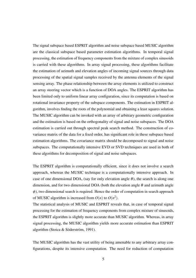
1.2 MANETs with Directional Antennas . . . . . . . . . . . . . . . . . . . . . . 4
2.1 Antenna Radiation Pattern (Balanis, 2012) . . . . . . . . . . . . . . . . . . . 13
2.2 Coordinate System for Antenna Analysis (Balanis, 2012) . . . . . . . . . . . 14
2.3 E and H Fields in Far-Field . . . . . . . . . . . . . . . . . . . . . . . . . . . 15
2.4 Veritical E-Fields Orientation of Rectangular Wave Guide - Vertical Polarization 15
2.5 Horizontal E-Fields Orientation of (RWG) - Horizontal Polarization . . . . . 16
2.6 Broadside Illumination of Sources . . . . . . . . . . . . . . . . . . . . . . . 17
2.7 Endfire Illumination of Sources . . . . . . . . . . . . . . . . . . . . . . . . . 17
2.8 Array Factor Parameters on Planar Array(Balanis, 2012) . . . . . . . . . . . 18
2.9 Point Source Spacing . . . . . . . . . . . . . . . . . . . . . . . . . . . . . . 21
2.10 Rectangular Waveguide Element Spacing . . . . . . . . . . . . . . . . . . . 21
2.11 Uniform Linear Array . . . . . . . . . . . . . . . . . . . . . . . . . . . . . . 22
2.12 Uniform Planar Array Configuration . . . . . . . . . . . . . . . . . . . . . . 23
2.13 Uniform Circular Array Configuration . . . . . . . . . . . . . . . . . . . . . 24
2.14 Cross Array Configuration (Hu, Zhang, & Wang, 2014) . . . . . . . . . . . . 25
2.15 Orthogonal Array Configuration (N. A.-H. M. Tayem, 2005) . . . . . . . . . 25
2.16 L Shaped Array Configuration (N. A.-H. M. Tayem, 2005) . . . . . . . . . . 27
2.17 One L Shaped Array Configuration (N. A.-H. M. Tayem, 2005) . . . . . . . . 27
2.18 Two L Shaped Array Configuration (N. A.-H. M. Tayem, 2005) . . . . . . . . 28
2.19 Block Diagram for DOA Using the MUSIC Algorithm . . . . . . . . . . . . 38
2.20 Non-Overlapping Subarrays . . . . . . . . . . . . . . . . . . . . . . . . . . 39
2.21 Overlapping Subarrays . . . . . . . . . . . . . . . . . . . . . . . . . . . . . 39
2.22 Mutually Orthogonal Arrangement of Dipoles (Chick, Collins, Goodman,
Martin, & Terzuoli Jr, 2011) . . . . . . . . . . . . . . . . . . . . . . . . . . 44
2.23 Mutually Orthogonal Arrangement of Antennas (Chick et al., 2011) . . . . . 44
2.24 3 Axis Orthogonal Antenna (M. Kim, Takeuchi, & Chong, 2004) . . . . . . . 45
xii
2.25 12-Element Array Antenna for Orthogonal Polarization Discrimination (Yoshimura,
Ushijima, Nishiyama, & Aikawa, 2011) . . . . . . . . . . . . . . . . . . . . 46
2.26 Antenna Array Behaviour with Schematic Current Distributions (Yoshimura et
al., 2011) . . . . . . . . . . . . . . . . . . . . . . . . . . . . . . . . . . . . 47
2.27 Narrowband and Wideband Signal Sources . . . . . . . . . . . . . . . . . . . 50
3.1 Rectangular Waveguide . . . . . . . . . . . . . . . . . . . . . . . . . . . . . 61
3.2 Circular Waveguide . . . . . . . . . . . . . . . . . . . . . . . . . . . . . . . 62
3.3 Normalized Radiation Pattern of a RWG . . . . . . . . . . . . . . . . . . . . 62
3.4 Co-polar and Cross Polar Radiation Pattern of a RWG . . . . . . . . . . . . . 63
3.5 Proposed Orthogonally Polarized Linear Array . . . . . . . . . . . . . . . . 63
3.6 Orthogonally Polarized Linear Array Configuration using RWG Elements . . 64
3.7 Polarization of RWG . . . . . . . . . . . . . . . . . . . . . . . . . . . . . . 65
3.8 Estimation of Angle θ through the peak of One-Dimensional Search Technique
for the DOA (−20◦,25◦) . . . . . . . . . . . . . . . . . . . . . . . . . . . . 70
3.9 RMSE Plot for Estimation of θ and φ angle using One Dimensional Search
Approach . . . . . . . . . . . . . . . . . . . . . . . . . . . . . . . . . . . . 75
3.10 RMSE Plot for Estimation of θ and φ angle using 2x2 Planar Array with
Conventioanl 2D-MUSIC . . . . . . . . . . . . . . . . . . . . . . . . . . . . 75
4.1 Conventional UPA . . . . . . . . . . . . . . . . . . . . . . . . . . . . . . . . 81
4.2 Orthogonal Polarized Planar Array . . . . . . . . . . . . . . . . . . . . . . . 81
4.3 Orthogonal Mounted Linear Array . . . . . . . . . . . . . . . . . . . . . . . 82
4.4 Orthogonally Polarized Linear Array . . . . . . . . . . . . . . . . . . . . . . 83
4.5 RMSE of Elevation Angle Estimation for Broadside Illumination at (35◦,25◦)
for UPA and OPPA Configurations . . . . . . . . . . . . . . . . . . . . . . . 84
4.6 RMSE of Elevation Angle Estimation for Broadside Illumination at (35◦,25◦)
for OMLA and OPLA Configurations . . . . . . . . . . . . . . . . . . . . . 85
4.7 RMSE of Azimuth Angle Estimation for Broadside Illumination at (35◦,25◦)
for UPA and OPPA Configurations . . . . . . . . . . . . . . . . . . . . . . . 86
4.8 RMSE of Azimuth Angle Estimation for Broadside Illumination at (35◦,25◦)
for OMLA and OPLA Configurations . . . . . . . . . . . . . . . . . . . . . 86
4.9 RMSE of Elevation Angle Estimation for End-fire Illumination at (60◦,60◦)
for UPA and OPPA Configurations . . . . . . . . . . . . . . . . . . . . . . . 88
xiii

4.10 RMSE of Elevation Angle Estimation for End-fire Illumination at (60◦,60◦)
for OMLA and OPLA Configurations . . . . . . . . . . . . . . . . . . . . . 88
4.11 RMSE of Azimuth Angle Estimation for End-fire Illumination at (60◦,60◦)
for UPA and OPPA Configurations . . . . . . . . . . . . . . . . . . . . . . . 89
4.12 RMSE of Azimuth Angle Estimation for End-fire Illumination at (60◦,60◦)
for OMLA and OPLA Configurations . . . . . . . . . . . . . . . . . . . . . 89
4.13 Two Dimensional DOA Estimation of Two Sources using UPA for 20 dB SNR 91
4.14 Two Dimensional DOA Estimation of Two Sources using OPPA for 20 dB SNR 92
4.15 Two Dimensional DOA Estimation of Two Sources using OMLA for 20 dB SNR 93
4.16 Two Dimensional DOA Estimation of Two Sources using OPLA for 20 dB SNR 93
4.17 Two Dimensional DOA Estimation of Two Sources using UPA for 10 dB SNR 95
4.18 Two Dimensional DOA Estimation of Two Sources using OPPA for 10 dB SNR 95
4.19 Two Dimensional DOA Estimation of Two Sources using OMLA for 10 dB SNR 96
4.20 Two Dimensional DOA Estimation of Two Sources using OPLA for 10 dB SNR 96
4.21 Two Dimensional DOA Estimation of Two Sources using UPA for 0 dB SNR 97
4.22 Two Dimensional DOA Estimation of Two Sources using OPPA for 0 dB SNR 98
4.23 Two Dimensional DOA Estimation of Two Sources using OMLA for 0 dB SNR 98
4.24 Two Dimensional DOA Estimation of Two Sources using OPLA for 0 dB SNR 99
4.25 Eigenvalue Spread for Two Sources SNR = 20 dB . . . . . . . . . . . . . . . 100
4.26 Eigenvalue Spread for Two Sources SNR = 10 dB . . . . . . . . . . . . . . . 101
4.27 Eigenvalue Spread for Two Sources SNR = 5 dB . . . . . . . . . . . . . . . . 102
4.28 Eigenvalue Spread for Two Sources SNR = 0 dB . . . . . . . . . . . . . . . . 102
4.29 Two Dimensional DOA Estimation of Three Sources using UPA for 0 dB SNR 104
4.30 Two Dimensional DOA Estimation of Three Sources using OPPA for 0 dB SNR105
4.31 Two Dimensional DOA Estimation of Three Sources using OMLA configura-
tion for 0 dB SNR . . . . . . . . . . . . . . . . . . . . . . . . . . . . . . . . 105
4.32 Two Dimensional DOA Estimation of Three Sources using OPLA for 0 dB SNR106
4.33 2D-DOA Estimation using UPA Configuration for Two Sources at (25◦,25◦)
and (45◦,45◦) for SNR of 10dB . . . . . . . . . . . . . . . . . . . . . . . . 108
4.34 2D-DOA Estimation using OPPA Configuration for Two Sources at (25◦,25◦)
and (45◦,45◦) for SNR of 10dB . . . . . . . . . . . . . . . . . . . . . . . . 108
4.35 2D-DOA Estimation using OMLA Configuration for Two Sources at (25◦,25◦))
and (45◦,45◦) for SNR of 10dB . . . . . . . . . . . . . . . . . . . . . . . . 109
xiv

4.36 2D-DOA Estimation using OPLA Configuration for Two Sources at (25◦,25◦)
and (45◦,45◦) for SNR of 10dB . . . . . . . . . . . . . . . . . . . . . . . . 109
4.37 2D-DOA Estimation of Closely Spaced Sources Estimation using UPA for
Two Sources at (25◦,25◦) and (25◦,35◦) . . . . . . . . . . . . . . . . . . . 110
4.38 2D-DOA Estimation of Closely Spaced Sources Estimation using UPA for
Two Sources at (25◦,25◦) and (25◦,40◦) . . . . . . . . . . . . . . . . . . . 111
4.39 2D-DOA Estimation of Closely Spaced Sources Estimation using UPA for
Two Sources at (25◦,25◦) and (25◦,43◦) . . . . . . . . . . . . . . . . . . . 111
4.40 2D-DOA Estimation of Closely Spaced Sources Estimation using OPPA for
Two Sources at (25◦,25◦) and (25◦,33◦) . . . . . . . . . . . . . . . . . . . 112
4.41 2D-DOA Estimation of Closely Spaced Sources Estimation using OPPA for
Two Sources at (25◦,25◦) and (25◦,35◦) . . . . . . . . . . . . . . . . . . . 113
4.42 2D-DOA Estimation of Closely Spaced Sources Estimation using OMLA for
Two Sources at (25◦,25◦) and (25◦,33◦) . . . . . . . . . . . . . . . . . . . 114
4.43 2D-DOA Estimation of Closely Spaced Sources Estimation using OMLA for
Two Sources at (25◦,25◦) and (25◦,34◦) . . . . . . . . . . . . . . . . . . . 114
4.44 2D-DOA Estimation of Closely Spaced Sources Estimation using OMLA for
Two Sources at (25◦,25◦) and (25◦,35◦) . . . . . . . . . . . . . . . . . . . 115
4.45 2D-DOA Estimation of Closely Spaced Sources Estimation using OPLA for
Two Sources at (25◦,15◦) and (25◦,40◦) . . . . . . . . . . . . . . . . . . . 116
4.46 2D-DOA Estimation of Closely Spaced Sources Estimation using OPLA for
Two Sources at (25◦,20◦) and (25◦,40◦) . . . . . . . . . . . . . . . . . . . 117
4.47 2D-DOA Estimation of Closely Spaced Sources Estimation using OPLA for
Two Sources at (25◦,25◦) and (15◦,45◦) . . . . . . . . . . . . . . . . . . . 117
4.48 Closely Spaced Sources Estimation using OPLA for Two Sources at (25◦,25◦)
and (25◦,40◦) . . . . . . . . . . . . . . . . . . . . . . . . . . . . . . . . . . 118
4.49 Estimation of DOA using OPLA for Two Sources at (25◦,25◦) and (25◦,35◦)
with d = 5.56cm . . . . . . . . . . . . . . . . . . . . . . . . . . . . . . . . . 119
4.50 Estimation of DOA using OPLA for Two Sources at (25◦,25◦) and (25◦,35◦)
with d = 11.2cm . . . . . . . . . . . . . . . . . . . . . . . . . . . . . . . . . 119
5.1 DOA Tracking by Instantaneous Samples Processed for SNR = 0 dB . . . . . 127
5.2 DOA Tracking by Weighting Factor Method α = 0.6 for SNR = 0 dB . . . . . 128
5.3 DOA Tracking by Forgetting Factor Method β = 0.95 q = 5 for SNR = 0 dB . 128
xv
5.4 Analysis of Weighting Factor in 2D-DOA Tracking . . . . . . . . . . . . . . 130
5.5 Analysis of Forgetting Factor in θ Estimation of 2D-DOA Tracking with
Orthogonal Polarized Linear Array . . . . . . . . . . . . . . . . . . . . . . . 131
5.6 Analysis of Forgetting Factor in φ Estimation of 2D-DOA Tracking with
Orthogonal Polarized Linear Array . . . . . . . . . . . . . . . . . . . . . . . 131
5.7 2D-DOA Tracking with Uniform Planar Array with Instantaneous Samples
with SNR 20 dB, θmse = 0.0826 and φmse = 0.1304 . . . . . . . . . . . . . . 133
5.8 2D-DOA Tracking with Uniform Planar Array with Weighting Factor with
SNR 20 dB, θmse = 0.0559 and φmse = 0.0939 . . . . . . . . . . . . . . . . 134
5.9 2D-DOA Tracking with Uniform Planar Array with Forgetting Factor with
SNR 20 dB, θmse = 0.0426 and φmse = 0.0919 . . . . . . . . . . . . . . . . 135
5.10 2D-DOA Tracking with Orthogonal Polarized Planar Array with Instantaneous
Samples with 20 dB SNR, θmse = 0.0499 and φmse = 0.0559 . . . . . . . . . 136
5.11 2D-DOA Tracking with Orthogonal Polarized Planar Array with Weighting
Factor 20 dB SNR, θmse = 0.0389 and φmse = 0.0450 . . . . . . . . . . . . . 137
5.12 2D-DOA Tracking with Orthogonal Polarized Planar Array with Forgetting
Factor 20 dB SNR, θmse = 0.0380 and φmse = 0.0622 . . . . . . . . . . . . . 138
5.13 2D-DOA Tracking with Orthogonal Mounted Linear Array with Instantaneous
Samples with 20 dB SNR, θmse = 0.0499 and φmse = 0.0559 . . . . . . . . . 140
5.14 2D-DOA Tracking with Orthogonal Mounted Linear Array with Weighting
Factor 20 dB SNR, θmse = 0.0389 and φmse = 0.0450 . . . . . . . . . . . . . 141
5.15 2D-DOA Tracking with Orthogonal Mounted Linear Array with Forgetting
Factor 20 dB SNR, θmse = 0.0380 and φmse = 0.0622 . . . . . . . . . . . . . 142
5.16 2D-DOA Tracking with Orthogonal Polarized Linear Array with Instantaneous
Samples with 20 dB SNR, θmse = 0.1386 and φmse = 0.1351 . . . . . . . . . 143
5.17 2D-DOA Tracking with Orthogonal Polarized Linear Array with Weighting
Factor 20 dB SNR, θmse = 0.0843 and φmse = 0.0994 . . . . . . . . . . . . . 144
5.18 2D-DOA Tracking with Orthogonal Polarized Linear Array with Forgetting
Factor 20 dB SNR, θmse = 0.0515 and φmse = 0.0952 . . . . . . . . . . . . . 145
5.19 Comparison of MSE of θ Estimation using Instantaneous Samples . . . . . . 146
5.20 Comparison of MSE of φ Estimation using Instantaneous Samples . . . . . . 147
5.21 Comparison of MSE of θ Estimation using Weighting Factor . . . . . . . . . 148
5.22 Comparison of MSE of φ Estimation using Weighting Factor . . . . . . . . . 148
5.23 Comparison of MSE of θ Estimation using Forgetting Factor . . . . . . . . . 150
xvi
5.24 Comparison of MSE of φ Estimation using Forgetting Factor . . . . . . . . . 150
6.1 Two Subband Approach for Wideband DOA Estimation . . . . . . . . . . . . 155
6.2 Two Subband Filters for Subband Technique . . . . . . . . . . . . . . . . . . 156
6.3 Wideband Source with Frequency Spread . . . . . . . . . . . . . . . . . . . 157
6.4 Wideband Source Mapped to Discrete Frequencies . . . . . . . . . . . . . . 158
6.5 Wideband DOA Estimation with Discrete Frequencies of Incoherent Method
with 30 dB SNR . . . . . . . . . . . . . . . . . . . . . . . . . . . . . . . . . 158
6.6 Wideband DOA Estimation with Discrete Frequencies of Incoherent Method
with 20 dB SNR . . . . . . . . . . . . . . . . . . . . . . . . . . . . . . . . . 159
6.7 Wideband DOA Estimation with Incoherent Method with 20 dB SNR . . . . 160
6.8 Wideband DOA Estimation with Discrete Frequencies of Incoherent Method
with 10 dB SNR . . . . . . . . . . . . . . . . . . . . . . . . . . . . . . . . . 160
6.9 Wideband DOA Estimation with CSSM Method for various SNRs . . . . . . 161
6.10 Wideband DOA Estimation with Subband Technique with 20 dB SNR . . . . 163
6.11 Wideband DOA Estimation with Subband Technique with 10 dB SNR . . . . 164
6.12 Wideband DOA Estimation with Subband Technique with 5 dB SNR . . . . . 164
6.13 Wideband DOA Estimation with Subband Technique with 0 dB SNR . . . . . 165
6.14 Comparison of Wideband DOA Estimation with 30 dB SNR . . . . . . . . . 166
6.15 Comparison of Wideband DOA Estimation with 30 dB SNR . . . . . . . . . 167
6.16 Comparison of Wideband DOA Estimation with 20 dB SNR . . . . . . . . . 167
6.17 Comparison of Wideband DOA Estimation with 10 dB SNR . . . . . . . . . 168
6.18 Comparison of Wideband DOA Estimation with 0 dB SNR . . . . . . . . . . 169
6.19 DOA Estimation of Two Wideband Sources with the Signal Model θ1 = 10◦,
and θ2 = 40◦ for 30 dB SNR . . . . . . . . . . . . . . . . . . . . . . . . . . 171
6.20 DOA Estimation of Two Wideband Sources with the Signal Model θ1 = 10◦,
and θ2 = 40◦ for 10 dB SNR . . . . . . . . . . . . . . . . . . . . . . . . . . 171
6.21 DOA Estimation of Two Wideband Sources with the Signal Model θ1 = 10◦,
and θ2 = 40◦ for 0 dB SNR . . . . . . . . . . . . . . . . . . . . . . . . . . . 172
6.22 DOA Estimation of Two Wideband Sources with the Signal Model θ1 =−10◦,
and θ2 = 20◦ for 30 dB SNR . . . . . . . . . . . . . . . . . . . . . . . . . . 173
6.23 DOA Estimation of Two Wideband Sources with the Signal Model θ1 =−10◦,
and θ2 = 20◦ for 10 dB SNR . . . . . . . . . . . . . . . . . . . . . . . . . . 174
xvii
6.24 DOA Estimation of Two Wideband Sources with the Signal Model θ1 =−10◦,
and θ2 = 20◦ for 0 dB SNR . . . . . . . . . . . . . . . . . . . . . . . . . . . 174
6.25 DOA Estimation of Two Wideband Sources with the Signal Model θ1 =−30◦,
and θ2 = 40◦ for 30 dB SNR . . . . . . . . . . . . . . . . . . . . . . . . . . 175
6.26 DOA Estimation of Two Wideband Sources with the Signal Model θ1 =−30◦,
and θ2 = 40◦ for 10 dB SNR . . . . . . . . . . . . . . . . . . . . . . . . . . 176
6.27 DOA Estimation of Two Wideband Sources with the Signal Model θ1 =−30◦,
and θ2 = 40◦ for 0 dB SNR . . . . . . . . . . . . . . . . . . . . . . . . . . . 176
6.28 2D-DOA Estimation of Wideband Sources with Uniform Planar Array for the
Signal Model θ = 15◦ and φ = 30◦ for 0 dB SNR . . . . . . . . . . . . . . . 179
6.29 2D-DOA Estimation of Wideband Sources with Uniform Planar Array for the
Signal Model θ = 15◦ and φ = 30◦ for 0 dB SNR - 2D View of Simulation
Result . . . . . . . . . . . . . . . . . . . . . . . . . . . . . . . . . . . . . . 179
6.30 2D-DOA Estimation of Wideband Sources with Orthogonal Polarized Planar
Array for the Signal Model θ = 15◦ and φ = 30◦ for 0 dB SNR . . . . . . . . 180
6.31 2D-DOA Estimation of Wideband Sources with Orthogonal Polarized Planar
Array for the Signal Model θ = 15◦ and φ = 30◦ for 0 dB SNR - 2D View of
Simulation Result . . . . . . . . . . . . . . . . . . . . . . . . . . . . . . . . 181
6.32 2D-DOA Estimation of Wideband Sources with Orthogonal Mounted Linear
Array for the Signal Model θ = 15◦ and φ = 30◦ for 0 dB SNR . . . . . . . . 182
6.33 2D-DOA Estimation of Wideband Sources with Orthogonal Mounted Linear
Array for the Signal Model θ = 15◦ and φ = 30◦ for 0 dB SNR - 2D View of
Simulation Result . . . . . . . . . . . . . . . . . . . . . . . . . . . . . . . . 182
6.34 2D-DOA Estimation of Wideband Sources with Orthogonal Polarized Linear
Array for the Signal Model θ = 15◦ and φ = 30◦ for 0 dB SNR . . . . . . . . 183
6.35 2D-DOA Estimation of Wideband Sources with Orthogonal Polarized Linear
Array for the Signal Model θ = 15◦ and φ = 30◦ for 0 dB SNR - 2D View of
Simulation Result . . . . . . . . . . . . . . . . . . . . . . . . . . . . . . . . 184
6.36 RMSE Comparison for θ Angle Estimation of 2D-DOA Estimation of Wide-
band Signal for Single and Orthogonal Polarized Array Configurations . . . . 185
6.37 RMSE Comparison for φ Angle Estimation of 2D-DOA Estimation of Wide-
band Signal for Single and Orthogonal Polarized Array Configurations . . . . 186
6.38 2D-DOA Estimation of Two Wideband Sources with Uniform Planar Array for
the Signal Model (θ1 = 52◦ , φ1 = 28◦) and (θ2 = 40◦ , φ2 = 65◦) for 0 dB SNR187
xviii

6.39 2D-DOA Estimation of Two Wideband Sources with Uniform Planar Array
for the Signal Model (θ1 = 52◦ , φ1 = 28◦) and (θ2 = 40◦ , φ2 = 65◦) for 0
dB SNR - 2D View of Simulation Result . . . . . . . . . . . . . . . . . . . . 188
6.40 2D-DOA Estimation of Two Wideband Sources with Orthogonal Polarized
Planar Array for the Signal Model (θ1 = 52◦ , φ1 = 28◦) and (θ2 = 40◦ ,
φ2 = 65◦) for 0 dB SNR . . . . . . . . . . . . . . . . . . . . . . . . . . . . . 189
6.41 2D-DOA Estimation of Two Wideband Sources with Orthogonal Polarized
Planar Array for the Signal Model (θ1 = 52◦ , φ1 = 28◦) and (θ2 = 40◦ ,
φ2 = 65◦) for 0 dB SNR - 2D View of Simulation Result . . . . . . . . . . . 189
6.42 2D-DOA Estimation of Two Wideband Sources with Orthogonal Mounted
Linear Array for the Signal Model (θ1 = 52◦ , φ1 = 28◦) and (θ2 = 40◦ ,
φ2 = 65◦) for 0 dB SNR . . . . . . . . . . . . . . . . . . . . . . . . . . . . . 190
6.43 2D-DOA Estimation of Two Wideband Sources with Orthogonal Mounted
Linear Array for the Signal Model (θ1 = 52◦ , φ1 = 28◦) and (θ2 = 40◦ ,
φ2 = 65◦) for 0 dB SNR - 2D View of Simulation Result . . . . . . . . . . . 191
6.44 2D-DOA Estimation of Two Wideband Sources with Orthogonal Polarized
Linear Array for the Signal Model (θ1 = 52◦ , φ1 = 28◦) and (θ2 = 40◦ ,
φ2 = 65◦) for 0 dB SNR . . . . . . . . . . . . . . . . . . . . . . . . . . . . . 192
6.45 2D-DOA Estimation of Two Wideband Sources with Orthogonal Polarized
Linear Array for the Signal Model (θ1 = 52◦ , φ1 = 28◦) and (θ2 = 40◦ ,
φ2 = 65◦) for 0 dB SNR - 2D View of Simulation Result . . . . . . . . . . . 192
A.1 Mutual Coupling of Rectangular Waveguide Array for Conventional Linear
Arrangement for Two Elements . . . . . . . . . . . . . . . . . . . . . . . . . 203
A.2 Mutual Coupling of Rectangular Waveguide Array for Orthogonal Arrange-
ment for Two Elements . . . . . . . . . . . . . . . . . . . . . . . . . . . . . 204
B.1 2D DOA Estimation of Single Wideband Source with UPA for the Signal
Model θ = 15◦ and φ = 30◦ for 10 dB SNR . . . . . . . . . . . . . . . . . . 207
B.2 2D DOA Estimation of Single Wideband Source with UPA for the Signal
Model θ = 15◦ and φ = 30◦ for 10 dB SNR - 2D View of Simulation Result . 207
B.3 2D DOA Estimation of Single Wideband Source with UPA for the Signal
Model θ = 15◦ and φ = 30◦ for 20 dB SNR . . . . . . . . . . . . . . . . . . 208
B.4 2D DOA Estimation of Single Wideband Source with UPA for the Signal
Model θ = 15◦ and φ = 30◦ for 20 dB SNR - 2D View of Simulation Result . 208
xix
B.5 2D DOA Estimation of Single Wideband Source with UPA for the Signal
Model θ = 15◦ and φ = 30◦ for 30 dB SNR . . . . . . . . . . . . . . . . . . 209
B.6 2D DOA Estimation of Single Wideband Source with UPA for the Signal
Model θ = 15◦ and φ = 30◦ for 30 dB SNR - 2D View of Simulation Result . 209
B.7 2D DOA Estimation of Single Wideband Source with OPPA for the Signal
Model θ = 15◦ and φ = 30◦ for 10 dB SNR . . . . . . . . . . . . . . . . . . 210
B.8 2D DOA Estimation of Single Wideband Source with OPPA for the Signal
Model θ = 15◦ and φ = 30◦ for 10 dB SNR - 2D View of Simulation Result . 210
B.9 2D DOA Estimation of Single Wideband Source with OPPA for the Signal
Model θ = 15◦ and φ = 30◦ for 20 dB SNR . . . . . . . . . . . . . . . . . . 211
B.10 2D DOA Estimation of Single Wideband Source with OPPA for the Signal
Model θ = 15◦ and φ = 30◦ for 20 dB SNR - 2D View of Simulation Result . 211
B.11 2D DOA Estimation of Single Wideband Source with OPPA for the Signal
Model θ = 15◦ and φ = 30◦ for 30 dB SNR . . . . . . . . . . . . . . . . . . 212
B.12 2D DOA Estimation of Single Wideband Source with OPPA for the Signal
Model θ = 15◦ and φ = 30◦ for 30 dB SNR - 2D View of Simulation Result . 212
B.13 2D DOA Estimation of Single Wideband Source with OMLA for the Signal
Model θ = 15◦ and φ = 30◦ for 10 dB SNR . . . . . . . . . . . . . . . . . . 213
B.14 2D DOA Estimation of Single Wideband Source with OMLA for the Signal
Model θ = 15◦ and φ = 30◦ for 10 dB SNR - 2D View of Simulation Result . 213
B.15 2D DOA Estimation of Single Wideband Source with OMLA for the Signal
Model θ = 15◦ and φ = 30◦ for 20 dB SNR . . . . . . . . . . . . . . . . . . 214
B.16 2D DOA Estimation of Single Wideband Source with OMLA for the Signal
Model θ = 15◦ and φ = 30◦ for 20 dB SNR - 2D View of Simulation Result . 214
B.17 2D DOA Estimation of Single Wideband Source with OMLA for Signal Model
θ = 15◦ and φ = 30◦ for 30 dB SNR . . . . . . . . . . . . . . . . . . . . . . 215
B.18 2D DOA Estimation of Single Wideband Source with OMLA for the Signal
Model θ = 15◦ and φ = 30◦ for 30 dB SNR - 2D View of Simulation Result . 215
B.19 2D DOA Estimation of Single Wideband Source with OPLA for the Signal
Model θ = 15◦ and φ = 30◦ for 10 dB SNR . . . . . . . . . . . . . . . . . . 216
B.20 2D DOA Estimation of Single Wideband Source with OPLA for the Signal
Model θ = 15◦ and φ = 30◦ for 10 dB SNR - 2D View of Simulation Result . 216
B.21 2D DOA Estimation of Single Wideband Source with OPLA for the Signal
Model θ = 15◦ and φ = 30◦ for 20 dB SNR . . . . . . . . . . . . . . . . . . 217
xx
B.22 2D DOA Estimation of Single Wideband Source with OPLA for the Signal
Model θ = 15◦ and φ = 30◦ for 20 dB SNR - 2D View of Simulation Result . 217
B.23 2D DOA Estimation of Single Wideband Source with OPLA for the Signal
Model θ = 15◦ and φ = 30◦ for 30 dB SNR . . . . . . . . . . . . . . . . . . 218
B.24 2D DOA Estimation of Single Wideband Source with OPLA for the Signal
Model θ = 15◦ and φ = 30◦ for 30 dB SNR - 2D View of Simulation Result . 218
C.2 2D DOA Estimation of Two Wideband Sources with UPA for the Signal Model
(θ1 = 52◦ , φ1 = 28◦) and (θ2 = 40◦ , φ2 = 65◦) for 10 dB SNR - 2D View of
Simulation Result . . . . . . . . . . . . . . . . . . . . . . . . . . . . . . . . 219
C.3 2D DOA Estimation of Two Wideband Sources with UPA for the Signal Model
(θ1 = 52◦ , φ1 = 28◦) and (θ2 = 40◦ , φ2 = 65◦) for 20 dB SNR . . . . . . . 220
C.4 2D DOA Estimation of Two Wideband Sources with UPA for the Signal Model
(θ1 = 52◦ , φ1 = 28◦) and (θ2 = 40◦ , φ2 = 65◦) for 20 dB SNR - 2D View of
Simulation Result . . . . . . . . . . . . . . . . . . . . . . . . . . . . . . . . 220
C.5 2D DOA Estimation of Two Wideband Sources with UPA for the Signal Model
(θ1 = 52◦ , φ1 = 28◦) and (θ2 = 40◦ , φ2 = 65◦) for 30 dB SNR . . . . . . . 221
C.6 2D DOA Estimation of Two Wideband Sources with UPA for the Signal Model
(θ1 = 52◦ , φ1 = 28◦) and (θ2 = 40◦ , φ2 = 65◦) for 30 dB SNR - 2D View of
Simulation Result . . . . . . . . . . . . . . . . . . . . . . . . . . . . . . . . 221
C.1 2D DOA Estimation of Two Wideband Sources with UPA for the Signal Model
(θ1 = 52◦ , φ1 = 28◦) and (θ2 = 40◦ , φ2 = 65◦) for 10 dB SNR . . . . . . . 222
C.7 2D DOA Estimation of Two Wideband Sources with OPPA for the Signal
Model (θ1 = 52◦ , φ1 = 28◦) and (θ2 = 40◦ , φ2 = 65◦) for 10 dB SNR . . . . 223
C.8 2D DOA Estimation of Two Wideband Sources with OPPA for the Signal
Model (θ1 = 52◦ , φ1 = 28◦) and (θ2 = 40◦ , φ2 = 65◦) for 10 dB SNR - 2D
View of Simulation Result . . . . . . . . . . . . . . . . . . . . . . . . . . . 223
C.9 2D DOA Estimation of Two Wideband Sources with OPPA for the Signal
Model (θ1 = 52◦ , φ1 = 28◦) and (θ2 = 40◦ , φ2 = 65◦) for 20 dB SNR . . . . 224
C.10 2D DOA Estimation of Two Wideband Sources with OPPA for the Signal
Model (θ1 = 52◦ , φ1 = 28◦) and (θ2 = 40◦ , φ2 = 65◦) for 20 dB SNR - 2D
View of Simulation Result . . . . . . . . . . . . . . . . . . . . . . . . . . . 224
C.11 2D DOA Estimation of Two Wideband Sources with OPPA for the Signal
Model (θ1 = 52◦ , φ1 = 28◦) and (θ2 = 40◦ , φ2 = 65◦) for 30 dB SNR . . . . 225
xxi

C.12 2D DOA Estimation of Two Wideband Sources with OPPA for the Signal
Model (θ1 = 52◦ , φ1 = 28◦) and (θ2 = 40◦ , φ2 = 65◦) for 30 dB SNR - 2D
View of Simulation Result . . . . . . . . . . . . . . . . . . . . . . . . . . . 225
C.13 2D DOA Estimation of Two Wideband Sources with OMLA for the Signal
Model (θ1 = 52◦ , φ1 = 28◦) and (θ2 = 40◦ , φ2 = 65◦) for 10 dB SNR . . . . 226
C.14 2D DOA Estimation of Two Wideband Sources with OMLA for the Signal
Model (θ1 = 52◦ , φ1 = 28◦) and (θ2 = 40◦ , φ2 = 65◦) for 10 dB SNR - 2D
View of Simulation Result . . . . . . . . . . . . . . . . . . . . . . . . . . . 226
C.15 2D DOA Estimation of Two Wideband Sources with OMLA for the Signal
Model (θ1 = 52◦ , φ1 = 28◦) and (θ2 = 40◦ , φ2 = 65◦) for 20 dB SNR . . . . 227
C.16 2D DOA Estimation of Two Wideband Sources with OMLA for the Signal
Model (θ1 = 52◦ , φ1 = 28◦) and (θ2 = 40◦ , φ2 = 65◦) for 20 dB SNR - 2D
View of Simulation Result . . . . . . . . . . . . . . . . . . . . . . . . . . . 227
C.17 2D DOA Estimation of Two Wideband Sources with OMLA for the Signal
Model (θ1 = 52◦ , φ1 = 28◦) and (θ2 = 40◦ , φ2 = 65◦) for 30 dB SNR . . . . 228
C.18 2D DOA Estimation of Two Wideband Sources with OMLA for the Signal
Model (θ1 = 52◦ , φ1 = 28◦) and (θ2 = 40◦ , φ2 = 65◦) for 30 dB SNR - 2D
View of Simulation Result . . . . . . . . . . . . . . . . . . . . . . . . . . . 228
C.19 2D DOA Estimation of Two Wideband Sources with OPLA for the Signal
Model (θ1 = 52◦ , φ1 = 28◦) and (θ2 = 40◦ , φ2 = 65◦) for 10 dB SNR . . . . 229
C.20 2D DOA Estimation of Two Wideband Sources with OPLA for the Signal
Model (θ1 = 52◦ , φ1 = 28◦) and (θ2 = 40◦ , φ2 = 65◦) for 10 dB SNR - 2D
View of Simulation Result . . . . . . . . . . . . . . . . . . . . . . . . . . . 229
C.21 2D DOA Estimation of Two Wideband Sources with OPLA for the Signal
Model (θ1 = 52◦ , φ1 = 28◦) and (θ2 = 40◦ , φ2 = 65◦) for 20 dB SNR . . . . 230
C.22 2D DOA Estimation of Two Wideband Sources with OPLA for the Signal
Model (θ1 = 52◦ , φ1 = 28◦) and (θ2 = 40◦ , φ2 = 65◦) for 20 dB SNR - 2D
View of Simulation Result . . . . . . . . . . . . . . . . . . . . . . . . . . . 230
C.23 2D DOA Estimation of Two Wideband Sources with OPLA for the Signal
Model (θ1 = 52◦ , φ1 = 28◦) and (θ2 = 40◦ , φ2 = 65◦) for 30 dB SNR . . . . 231
C.24 2D DOA Estimation of Two Wideband Sources with OPLA for the Signal
Model (θ1 = 52◦ , φ1 = 28◦) and (θ2 = 40◦ , φ2 = 65◦) for 30 dB SNR - 2D
View of Simulation Result . . . . . . . . . . . . . . . . . . . . . . . . . . . 231
xxii

Nomenclature
a - Width of the RWG (mm) or (cm)
b - Height of the RWG (mm) or (cm)
c - Electromagnetic Velocity (m/s)
d - Inter-element spacing (mm) or (cm)
ex - Exponential of x
f - Frequency (Hz) (MHz) (GHz)
j - Imaginary component of the complex term
k - Wave number
m - Index to denote mth antenna of the array
n - Index to denote nth sampling instant
p - Index to denote pth source
q - Order of the Smoothing Filter
t - Index to denote tth time instant
x - x coordinate
y - y coordinate
z - z coordinate
α - Weighting Factor
β - Forgetting Factor
βmn - Propagation Constant of RWG Exited in mode mn
λ - Wavelength (mm) or (cm) or (m)
λi - ith Eigenvalue
µ - Free Space Permeability
ε - Free Space Permittivity
ρ - Radius of CWG
θ - Elevation angle in Degrees
φ - Azimuth angle in Degrees
σi - ith Singular Value
σ2 - Noise variance
xxiii
ω - Angular Frequency
60◦ - Denoting 60 Degrees
E - E field of EM wave or E Plane
E(.) - Mathematical Expectation
H - H field of EM wave or H Plane
(.)H - Hermitian Conjugate (Transpose) of a Matrix
(.)T - Matrix Transpose
J1(.) - First Order Bessel Function
J′1(.) - Derivative of the First Order Bessel Function
M - Number of Antenna Elements in Array
N - Number of Samples
P - Number of Sources
Eφ (θ ,φ) - Vertical Polarized Component of Radiation Pattern
Eθ (θ ,φ) - Horizontal Polarized Component of Radiation Pattern
a - Array Steering Vector
x - Array Observation Vector
xh - Data Observation Vector from Antenna elements along H plane
xe - Data Observation Vector from Antenna elements along E plane
s - Signal Vector
v - Eigenvector
w - Additive White Gaussian Noise Vector
A - Array Steering Matrix
I - Identity Matrix
R - Covariance Matrix
S - Signal Data Matrix
Rxx - Covariance Matrix
Rs - Signal Covariance Matrix
U - Matrix with the columns of Left Singular Vectors
V - Matrix with the columns of Right Singular Vectors or Eigenvectors
Vn - Noise Subspace Matrix
Λ - Diagonal Matrix with Eigenvalues on Diagonal
Σ - Diagonal Matrix with Singular values on Diagonal
xxiv

List of Abbreviations
1D - One Dimension
2D - Two Dimension
3D - Three Dimension
dB - Decibel
mm - Millimetre
cm - Centimetre
AMI - Array Manifold Interpolation
AIC - Akaike Information Criterion
BER - Bit Error Rate
Bi-SVD - Bi Iteration Singular Value Decomposition
BWFN - Beamwidth Between First Null
CCM - Cross Covariance Matrix
CWG - Circular Waveguide
CSSM - Coherent Signal Subspace Method
DFS - Direction Finding System
DOA - Direction of Arrival
OPAST - Orthonormal Projection Approximation Subspace Tracking
EM - Electromagnetic
ESPRIT - Estimation of Signal Parameters via Rotational Invariance Technique
ETOPS - Extended Test of Orthogonality of Projected Subspaces
EVD - Eigen Value Decomposition
HPBW - Half Power Beamwidth
ICM - Incoherent Method
KFVM - Kalman Filter with a Variable Number of Measurements
MAC - Multiply Accumulate
MANET - Mobile Ad-Hoc Network
MDL - Minimum Description Length
ME - Maximum Entropy
xxv

ML - Maximum Likelihood
MPAST - Modified Projection Approximation Subspace Tracking
MSE - Mean Square Error
MUSIC - Multiple Signal Classification
MVDR - Minimum Variance Distortionless Response
NS - Noise Subspace
OMLA - Orthogonal Mounted Linear Array
OPLA - Orthogonal Polarized Linear Array
OPPA - Orthogonal Polarized Planar Array
PAST - Projection Approximation Subspace Tracking
PM - Propagator Method
RF - Radio Frequency
RFID - Radio Frequency Identification
RLS - Recursive Least Squares
RWG - Rectangular Waveguide
RMSE - Root Mean Square Error
R-CSM - Robust Coherent Signal Subspace Method
SLA - Sparse Linear Array
SVD - Singular Value Decomposition
SNR - Signal to Noise Ratio
SURE - Subspace Rotation Estimation
SS - Signal Subspace
SS-MUSIC- Spatial Smoothing MUSIC
SSS-MUSIC- Signal Subspace Scaled Multiple Signal Classification
TOPS - Test of Orthogonality of Projected Subspaces
ULA - Uniform Linear Array
UPA - Uniform Planar Array
UCA - Uniform Circular Array
WAVES - Weighted Average of Signal Subspaces
W-SpSF - Wideband Sparse Spectrum Fitting
xxvi

Chapter 1
Introduction
1.1 Introduction to DOA Estimation
Antenna array processing has been in the forefront during the last several decades catering
to the research progress of radar and wireless communication engineering. Estimation of
signal parameters has been a topic of considerable research interest to various disciplines
coming under the purview of communication systems designed to meet the system applica-
tions of radar and wireless technologies. The Direction of Arrival (DOA) is a technique for
the estimation of angular direction of the signal sources impinging on the array of sensing
elements by subjecting the received data samples to the array signal processing algorithms.
The localization of the impinging source (signal) on the array of sensor elements is the
theme of DOA estimation technique. The DOA estimation finds many applications in vari-
ous disciplines of engineering. In radar and communication engineering, sensing elements
are usually antennas which are part of the base station to identify the signals as well as
interference. The system which performs the DOA estimation is also widely referred to as
Direction Finding System (DFS).
Array signal processing is a broad field of research interest in advanced antenna systems.
Development of algorithms in array signal processing for advanced antenna techniques,
is of great relevance to wireless communication as well as radar engineering. The spatial
samples of the signals emitted from various sources are received by the antenna elements
of the array. The received data samples depend on the characteristics of the sources, the
channels, the noise, and the measurement devices. Typically, the data are processed to
estimate the parameters such as number of sources, location of sources, range or distance
as well as velocity of the moving sources of signals. Estimation of these parameters opens
up an avenue for a large number of studies involving different system models and signal
processing objectives. Over the past decades, many researchers have been fascinated by
the realisable novelties and niceties offered by the domain of estimation algorithm. The
1

demand for the performance enhancement of estimation algorithms has drawn attention and
focus of applied mathematicians and signal processing researchers. Many researchers have
attempted and contributed numerous techniques to this discipline. The source localization
using smart antennas is one such problem which has evolved from the classical direction
finding problem in radar signal processing. Through collection of received time samples
and by processing of spatial signals, detection of multiple incoming sources and estimation
of their DOAs can be realised (Krim & Viberg, 1996).
The spatial samples received through the elements of antenna array are processed to
estimate the DOA. The algorithms of earlier DOA estimation techniques were either
Fourier based or beamforming based. Later the arrival of subspace based approaches laid
foundation for the development of algorithms for DOA estimation with higher resolution.
The subspace algorithms are based on Eigen Value Decomposition (EVD) and Singular
Value Decomposition (SVD) techniques (Golub & Van Loan, 2012). EVD plays a crucial
role in signal processing, because it can split a mixture of complex signals into a set of
desired and undesired subspace components. Thus, eigen based methods have been exten-
sively researched in adaptive signal processing. These algorithms were initially developed
to find the one dimensional DOA and later extended for two dimensional DOA estimation.
1.2 Applications of DOA Estimation
The DOA estimations find utility in diversified system applications and the following are
a few examples, where DOA estimation schemes are employed (Van Trees, 2004) and
(J. C. Chen, Yao, & Hudson, 2002); RADAR systems installed as phased array radar and
air-traffic control radar; SONAR systems deploy DOA estimation schemes to estimate the
far-field sources with localization and classification. In mobile communications, smart
antennas with suitable adaptive signal processing sensor array are adopted. This technique
will be able to locate mobile users with the use of DOA estimation techniques. In radio
astronomy, the radio telescopes are used for the detection of radio waves from an astronom-
ical object or celestial bodies. The accuracy and resolution of DOA estimation algorithms
play a significant role. Seismology which deals with scientific study of earthquakes and
the propagation of elastic waves through the earth finds the utility of DOA estimation
algorithms to determine the origin of the seismic waves. In wireless communication,
multipath channel characteristics of radio channel can be analysed using DOA estimation
2
algorithms. The angle of arrival statistics and time of arrival statistics are incorporated in
channel models to characterise the multipath channels more accurately (Fuhl, Rossi, &
Bonek, 1997; Rappaport, Reed, & Woerner, 1996). Recently, DFS has been identified for
its potential in mobile communication systems for the characterisation of channel statistics
in a multipath scenario. The DOA of interfering signal can also be estimated using DFS.
The DOA estimation technique has paramount importance in tracking of signal sources
in civilian and commercial applications. The DOA technique is a multi specialization
entity embarking on the speciality domains of antenna engineering, algorithms of array
signal processing and estimation techniques of communication engineering (Chryssomallis,
2000).
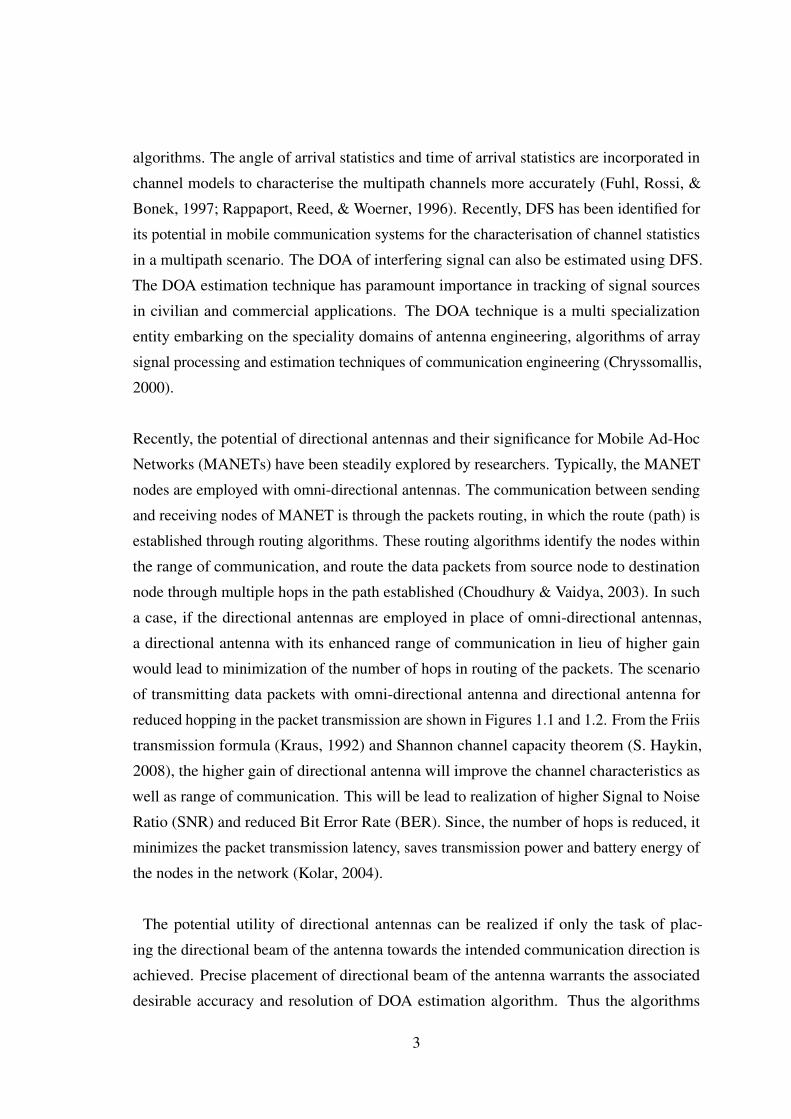
Recently, the potential of directional antennas and their significance for Mobile Ad-Hoc
Networks (MANETs) have been steadily explored by researchers. Typically, the MANET
nodes are employed with omni-directional antennas. The communication between sending
and receiving nodes of MANET is through the packets routing, in which the route (path) is
established through routing algorithms. These routing algorithms identify the nodes within
the range of communication, and route the data packets from source node to destination
node through multiple hops in the path established (Choudhury & Vaidya, 2003). In such
a case, if the directional antennas are employed in place of omni-directional antennas,
a directional antenna with its enhanced range of communication in lieu of higher gain
would lead to minimization of the number of hops in routing of the packets. The scenario
of transmitting data packets with omni-directional antenna and directional antenna for
reduced hopping in the packet transmission are shown in Figures 1.1 and 1.2. From the Friis
transmission formula (Kraus, 1992) and Shannon channel capacity theorem (S. Haykin,
2008), the higher gain of directional antenna will improve the channel characteristics as
well as range of communication. This will be lead to realization of higher Signal to Noise
Ratio (SNR) and reduced Bit Error Rate (BER). Since, the number of hops is reduced, it
minimizes the packet transmission latency, saves transmission power and battery energy of
the nodes in the network (Kolar, 2004).
The potential utility of directional antennas can be realized if only the task of plac-
ing the directional beam of the antenna towards the intended communication direction is
achieved. Precise placement of directional beam of the antenna warrants the associated
desirable accuracy and resolution of DOA estimation algorithm. Thus the algorithms
3
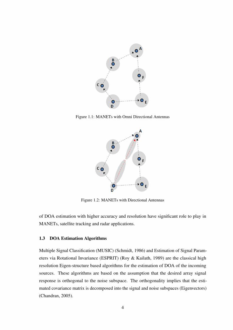
Figure 1.1: MANETs with Omni Directional Antennas
Figure 1.2: MANETs with Directional Antennas
of DOA estimation with higher accuracy and resolution have significant role to play in
MANETs, satellite tracking and radar applications.
1.3 DOA Estimation Algorithms
Multiple Signal Classification (MUSIC) (Schmidt, 1986) and Estimation of Signal Param-
eters via Rotational Invariance (ESPRIT) (Roy & Kailath, 1989) are the classical high
resolution Eigen-structure based algorithms for the estimation of DOA of the incoming
sources. These algorithms are based on the assumption that the desired array signal
response is orthogonal to the noise subspace. The orthogonality implies that the esti-
mated covariance matrix is decomposed into the signal and noise subspaces (Eigenvectors)
(Chandran, 2005).
4
The signal subspace based ESPRIT algorithm and noise subspace based MUSIC algorithm
are the classical subspace based parameter estimation algorithms. In temporal signal
processing, the estimation of frequency components from the mixture of complex sinusoids
is carried with these algorithms. In array signal processing, these algorithms facilitate
the estimation of azimuth and elevation angles of incoming signal sources through data
processing of the spatial signal samples received by the antenna elements of the signal
sensing array. The phase relationship between the array elements is utilized to construct
an array steering vector which is a function of DOA angles. The ESPRIT algorithm has
been limited only to uniform linear array configuration, since its computation is based on
rotational invariance property of the subspace components. The estimation in ESPRIT al-
gorithm, involves finding the roots of the polynomial and obtaining a least squares solution.
The MUSIC algorithm can be invoked with an array of arbitrary geometric configuration
and the estimation is based on the orthogonality of signal and noise subspaces. The DOA
estimation is carried out through spectral peak search method. The construction of co-
variance matrix of the data for a fixed order, has significant role in these subspace based
estimation algorithms. The covariance matrix should be decomposed to signal and noise
subspaces. The computationally intensive EVD or SVD techniques are used in both of
these algorithms for decomposition of signal and noise subspaces.
The ESPRIT algorithm is computationally efficient, since it does not involve a search
approach, whereas the MUSIC technique is a computationally intensive approach. In
case of one dimensional DOA, (say for only elevation angle θ ), the search is along one
dimension, and for two dimensional DOA (both the elevation angle θ and azimuth angle
φ ), two dimensional search is required. Hence the order of computation in search approach
of MUSIC algorithm is increased from O(n) to O(n2).
The statistical analysis of MUSIC and ESPRIT reveals that, in case of temporal signal
processing for the estimation of frequency components from complex mixture of sinusoids,
the ESPRIT algorithm is slightly more accurate than MUSIC algorithm. Whereas, in array
signal processing, the MUSIC algorithm yields more accurate estimation than ESPRIT
algorithm (Stoica & Soderstrom, 1991).
The MUSIC algorithm has the vast utility of being amenable to any arbitrary array con-
figurations, despite its intensive computation. The need for reduction of computation
5

in the MUSIC algorithm for array signal processing based parameter (DOA) estimation
problems is a single significant motivation factor to pursue research pertaining to estimation
algorithms. The conventional DFS utilizes an antenna array, in which the elements are
excited in single polarization. Typically, the performance of DOA estimation is studied
with an assumption of isotropic radiating elements in the antenna array. In this, the gain
of the antenna is assumed to be unity in all angles. The gain of the antenna element in
the array is not considered in the DOA estimation, since it will be a scaling factor that is
uniform across all the elements of the array. The assumption of unity gain of the antenna
elements is valid in DOA estimation involving spatial signal samples obtained through
single polarized antenna array with identical elements.
The scope of improving the estimation accuracy and resolution of MUSIC algorithm,
is yet another direction of research which encourages to design diversely polarized antenna
arrays. The antenna array with diversely polarized (vertical and horizontal polarization)
antenna elements will not have uniform gain across the array and hence the unity gain
assumption is not valid in such a case. Thus, the radiation pattern of individual antenna
elements of the array must be considered along with their respective polarization for esti-
mation of DOA angles of interest.
The difference in the gain of the vertical and horizontal polarized antenna elements present
in the diversely polarized antenna array provides a difference in the covariance of the
data received through the vertical and horizontal polarized array elements. The perfect
orthogonality between the signal and noise subspaces is expected in the decomposition of
the covariance matrix, which cannot occur in the practical scenario, because of the additive
noise present in the signal reception. The difference in the covariance of the data through
orthogonal polarized elements leads to the improved orthogonality between the signal and
noise subspace components accomplished through EVD or SVD of the covariance matrix of
the data samples. This improvement in the subspace decomposition directly reflects in the
improved estimation accuracy and resolution of the DOA angles. The improved accuracy
of DOA estimation from the diversely polarized array, warrants the analysis and design of
novel array configurations named as orthogonal polarized array configurations, with its
antenna elements having a combination of horizontal and vertical polarized elements in
different geometric configurations. These orthogonal polarized array configurations must
be evaluated for their performance in DOA estimation for wide range of SNR scenarios.
The correlation property associated with the covariance matrix of the data samples obtained
6

through the antenna elements of the diversely (orthogonally) polarized array configurations
is likely to not only improve the accuracy of the DOA estimation, but also the resolution to
distinguish the closely spaced sources.
The DOA estimation by classical algorithms such as MUSIC and ESPRIT for stationary
(fixed) sources is straight forward through the well established procedures. However the
non-stationary sources (moving sources) pose challenges in DOA estimation. In simple
terms, DOA tracking is nothing but estimation of DOA of non stationary sources and
tracking the movements of the sources. The dynamic changes in the moving sources lead
to fluctuations in the covariance of the data matrix as and when the (instantaneous) samples
are received. Hence, the sample covariance matrix is not the correct choice for DOA
estimation, whereas as a smoothing filter which does the weighted average of covariance
information from the current and past samples tends to improve the accuracy of DOA esti-
mation. The improved accuracy of 2D-DOA estimation with orthogonal polarized arrays,
along with the improved covariance matrix using smoothing filter can offer a cumulative
advantage in the tracking of 2D-DOA of non-stationary sources.
The term signal bandwidth is defined as the difference between the highest (significant)
frequency and the lowest (significant) frequency in the signal spectrum (Lathi, 1998). In a
wideband signal, the signal power spreads over wide range of frequencies. The spread of
signal power in a narrow band signal is limited to a narrow range of frequencies (S. Haykin,
2008). However the term bandwidth is relative with respect to which part of the EM
spectrum the signal is occupying.
Most signal sources used in wireless or mobile communication channels are not a nar-
row band signal. The information modulated by a carrier wave will always have a fixed
bandwidth. Such signals with a defined bandwidth are termed as wideband signals. The
terms wideband and broadband are sometimes interchangeably used in the broad domain
of communication engineering. The scope of the study in DOA estimation can be extended
to investigate the effect of orthogonal polarized array configurations for wideband source
scenarios. The phase difference between the array elements for narrow band signals is fixed,
whereas the corresponding phase difference of wideband signal gets cumulatively added
for every discrete frequency component present in the signal.The cumulative phase along
with the additive noise lead to increased complexity in the DOA estimation. Typically,
wideband DOA estimation is performed by processing the discrete frequency components
7
of a wide band signal. For the estimation of DOA of incoming wideband sources, the
classical techniques of incoherent and the coherent approaches are widely used. The
incoherent approach averages the DOA estimation from the all the subspace components
of the discrete frequencies. The coherent approach uses a transformation matrix to focus
the signal subspace components of every discrete frequency to a desired frequency. Sev-
eral methods of focussing the signal subspace components are proposed in the literature
(Di Claudio & Parisi, 2001; Sellone, 2006). The potential utility of conventional subband
filtering approach used in the multirate filters (Vaidyanathan, 1993) and image processing
(Woods & O’Neil, 1986) can be utilised for DOA estimation of wideband sources. The
improved DOA estimation using orthogonal polarized array configurations along with the
subband approach can be exploited to process the wideband signal, to enhance its capability
of 2D-DOA estimation. This simple subband approach does not involve any focusing of
subspace and will estimate the 2D-DOA of wideband in a consistent manner. The subband
filter approach is also preferred for its lower computational complexity when compared to
the conventional incoherent and coherent approaches.
1.4 Motivation of the Research
DFS as a whole is a multi-disciplinary domain. The DFS involves the antenna array, Radio
Frequency (RF) modules and digital signal processing modules to perform computation. In
the past, significant research work has been carried in the development of DOA estimation
algorithm, in an isolated way with a number of assumptions. Most of the research in DOA
estimation is oriented towards the development or improvement over the existing algo-
rithms with reduced emphasis on antenna configurations. The researchers have preferred to
deal the problem in an isolated way by assuming the isotropic elemental radiation pattern,
even though most commonly used elements of the antenna array are not omni antennas.
The simulation of DOA estimation algorithms with actual radiation pattern of antenna
element will be helpful to analyse its effects on the accuracy and resolution of DFS. The
study of DOA estimation with the consideration of elemental radiation pattern in turn can
affect the resolution of the estimation.
This thesis aims to focus its research on the DOA estimation emphasising techniques,
algorithms and approaches to improve the performance characteristics (resolution, accu-
racy) of the DOA estimation. In the framework of DOA estimation, several characteristics
8

play vital role in the performance of DFS system. They are
• Configuration of array and its elements
• Characteristics of the received signal
• Estimation Algorithm
A need for novel approaches in the 2D-DOA estimation technique with improved esti-
mation accuracy and resolution with lesser computational complexity is justifiable. The
requirement for improved signal processing algorithm suitable to track the 2D-DOA of the
non-stationary sources with least computation is also valid. A performance enhancement in
the estimation of 2D-DOA for the case of wideband signal sources will also be beneficial
from practical consideration. In this context, the following questions have been formed to
formulate the intended research pursuance.
1. Can different configurations of orthogonally polarized array be designed for improved
accuracy and resolution of 2D-DOA estimation algorithms?
2. Will the designed orthogonal polarized array configurations be able to resolve DOA
of multiple sources, if their angular separation between them is smaller?
3. Can the designed orthogonally polarized array configurations be utilized for effective
tracking of dynamic sources?
4. Will the proposed orthogonal polarized array configurations be effective to treat the
2D-DOA of single and multiple wideband sources
5. For the retention of orthogonally polarized elements for higher accuracy and resolu-
tion of 2D-DOA estimation, what modifications are needed at algorithmic perspec-
tives to make them more amenable for DOA estimation?
6. Is there a feasibility to reduce the computational complexity of the MUSIC algorithm
in 2D-DOA estimations?
1.5 Objectives of the Thesis
This thesis envisages to address the above listed research questions through the realization
of the following formulated objectives.
9
1. To review the literature pertaining to the DOA estimation algorithms, approaches
with respect to improve the resolution
2. To design, simulate and analyse the array of antenna elements with adjacent elements
orthogonally polarized
3. To develop a DOA estimation scheme using orthogonally polarized adjacent elements
4. To enhance the performance of subspace based DOA estimation techniques using
subspace tracking algorithms
5. To propose a novel approach for DOA estimation of wideband incoming signals
1.6 Organization of the Thesis
The subsequent chapters of this thesis are organized as follows.
• Chapter 2 is intended to facilitate a succinct and yet an effective review of background
theory of antennas, antenna array and various DOA estimation algorithms
• Chapter 3 deals with the novel linear array configuration with its alternate elements
orthogonally polarised and such an array is termed as Orthogonally Polarised Linear
Array (OPLA). A closed form solution for MUSIC based 2D-DOA estimation of
a single source is proposed which involves only 1D search instead of conventional
2D search. The computational advantage of the proposed 1D search scheme is
substantiated through relevant case studies.
• Chapter 4 proposes novel orthogonally polarised antenna array configurations which
enhance the accuracy and resolution of 2D-DOA of multiple sources compared with
conventional single polarized uniform planar array. This chapter also discusses
simulation results to substantiate the significant advantages of orthogonally polarised
antenna array configurations to distinguish the multiple sources with relatively
closer angular separation between them. This chapter also discusses a comparative
RMSE performance analysis of 2D-DOA estimation realised through the proposed
orthogonally polarised arrays and conventional single polarized planar array.
• Chapter 5 deals with the formulation and solution technique to analyse the tracking
behaviour of 2D-DOA estimation of dynamic sources using the proposed novel
10
orthogonally polarised antenna array configurations. In particular, this chapter
emphasises the importance of the techniques used for the formation of covariance
matrix of the data samples and their influence on the accuracy of 2D-DOA estimation.
• Chapter 6 presents an analysis for 2D-DOA estimation of wideband sources based on
an elegant subband filtering technique. The simulation studies presented in this chap-
ter substantiate the consistent and steady performance of subband based 2D-DOA
estimation of wideband sources at all SNR levels. This chapter also compares the
accuracy and resolution of 2D-DOA estimation realized through subband approach
with the conventional coherent and incoherent methods.
• Chapter 7 is aimed at the summary and significance of the analytical formulations
along with the associated simulation results presented in this thesis. The suggestions
for further research studies on the topics coming under the purview of this thesis are
also incorporated in this chapter.
11
Chapter 2
Review of Antenna Arrays and DOA Estimation Algorithms
This chapter intends to review the concepts of antennas, antenna array theory and various
antenna array configurations applicable for two dimensional DOA estimation. This chapter
also details the fundamental concepts of array signal processing and provides a detailed
review on classical algorithms for 2D-DOA estimation. The techniques and algorithms
required to extend conventional DOA estimation to dynamic sources are also covered in
this chapter. The analytical consideration and the algorithms in the 2D-DOA estimation to
deal with wideband sources are also presented in this chapter.
2.1 Antennas
An antenna facilitates the propagation of electromagnetic waves in free space. It is an
interface between free space EM waves propagation and a guided medium. An antenna
plays a significant role in the performance of wireless communication systems. The antenna
array has been a preferred solution for applications such as radar and communications.
Rapid technological progress in wireless communication has provided an impetus for
advancement of antenna engineering. The fundamental parameters and radiation behaviour
of the radiating elements are significant to facilitate a better understanding of antenna
arrays.
2.1.1 Radiation Pattern
The radiation pattern is a two or three-dimensional representation of radiation of an antenna.
According to the IEEE (“IEEE Standard Definitions of Terms for Antennas”, 1983) the
radiation pattern is defined as, A mathematical function or a graphical representation of
the radiation properties of the antenna as a function of space coordinates. This parameter
highly depends upon the application of the antenna.
The radiation pattern of an antenna can be depicted or illustrated through a two di-
mensional representation or three dimensional representation for a given distance of
12

measurement. In a two dimensional representation, the illustration is restricted to a particu-
lar plane of a given three dimensional space. For example, In a Cartesian measurement
system, the three dimensional representation corresponds to the three orthogonal axes x,
y and z. The radiation patterns of an antenna in xz, yz and xy planes correspond to two
dimensional representation. In a spherical polar coordinate system, the two dimensional
radiation pattern may correspond to a plane of a fixed θ and varying φ or vice versa. A
three dimensional radiation pattern of antenna in a spherical polar coordinate, corresponds
to the radiation pattern measured / computed for θ varying from 0◦ to 180◦ and φ varying
from 0◦ to 360◦.
The antenna radiation is measured in terms of a parameter called gain (dB). The antenna
gain is defined as, The ratio of the intensity, in a given direction, to the radiation intensity
that would be obtained if the power accepted by the antenna were radiated isotropically
(“IEEE Standard Definitions of Terms for Antennas”, 1983; Balanis, 2012). A plot of
radiation pattern of an antenna as a two dimensional graph is as shown in Figure 2.1. The
main beam of an antenna refers to the region of strong radiation from the antenna. The
maximum gain of the main lobe is termed as the peak gain of the antenna and side lobe
level of antenna determines the radiation in other directions.
Figure 2.1: Antenna Radiation Pattern (Balanis, 2012)
13
This item has been removed due to 3rd Party Copyright. The unabridged version of the thesis can be found in the Lancester
Library, Coventry University.

Figure 2.2: Coordinate System for Antenna Analysis (Balanis, 2012)
The radiation at exactly 180◦ from main lobe is called as back lobe. The Half Power
Beam Width (HPBW) is the width of main lobe between half power points. The Beam
Width between the First Nulls (BWFN) is a parameter measured as width of the mainlobe
between the first null of the left and right side of the mainlobe. The HPBW and BWFN
are the performance parameters to characterize the shape of the radiation pattern of the
antenna or antenna array (Balanis, 2012, 2011). A coordinate system for radiation pattern
analysis of an antenna is shown in Figure 2.2.
2.1.2 Antenna Polarization
Polarization is an important radiation characteristic of the antenna. In a broad sense an
antenna exhibits two polarizations typically called as vertical and horizontal polarization.
The Figure 2.3 shows that, in the far-field distance from a dipole antenna, the E-field
(E-wave or Electric field) oscillates. The H-field (H-wave or Magnetic field) also oscillates
14
This item has been removed due to 3rd Party Copyright. The unabridged version of the thesis can be found in the Lancester Library, Coventry University.
perpendicular to the E-field plane. Both E and H fields oscillate together along the
propagation axis. The direction of the electric field orientation of the antenna with respect
to a reference plane (typically azimuth) is referred as polarization of the antenna. In Figure
Figure 2.3: E and H Fields in Far-Field
Figure 2.4: Veritical E-Fields Orientation of Rectangular Wave Guide - Vertical Polarization
2.4, the E-field orientation is vertical. Thus an antenna is termed as a vertically polarized
antenna. If the orientation of the E-field of the antenna is horizontal as shown in Figure 2.5,
then the polarization of the antenna is horizontal. The mounting position of the antenna
also decides the polarization characteristics.
The radiation pattern of an antenna with linear polarization is discussed with respect
to the principal plane of interest. Typically, the principal planes are E or H planes. The
E-plane radiation pattern of the antenna corresponds to the radiation pattern in the plane
containing the E-field of aperture distribution and the direction of the wave propagation
(maximum radiation). Referring to Figure 2.4, the E-plane radiation pattern of the antenna
is measured in xz plane. Likewise, the H-plane radiation pattern of the antenna corresponds
15
This item has been removed due to 3rd Party Copyright. The unabridged version of the thesis can be found in the Lancester
Library, Coventry University.
This item has been removed due to 3rd Party Copyright. The unabridged version of the thesis can be found in the Lancester
Library, Coventry University.
Figure 2.5: Horizontal E-Fields Orientation of (RWG) - Horizontal Polarization
to the radiation pattern in the plane containing the H-field of aperture distribution and the
direction of wave propagation (maximum radiation). Referring to Figure 2.4, the H-plane
of the radiation pattern of the antenna is measured in yz plane. Mostly, antennas are oriented
to one of the principal planes where the antenna maximum radiation is coincident with it
(Balanis, 2012; Allen & Ghavami, 2006).
The concepts of the dual polarization characteristics and dual polarized antenna are often
misunderstood and interchangeably used in practice. A single antenna radiator fed with a
single feed, that exhibits both the horizontal and vertical polarized components of equal or
comparable amplitude in a plane (either azimuth or elevation) is called a dual polarized
antenna. Any conventional antenna radiating in single polarization (say vertical) can be
physically rotated by 90◦ (about its propagation (z) axis) to receive the other orthogonal
polarized (horizontal) component of the signal. In such a case, the antenna should not be
called as dual polarized antenna.
2.1.3 Illumination of Sources
The impinging angles (θ ,φ) of a source on the array of antenna elements are classified as
broad side illumination and endfire illumination. In antenna elements such as waveguides
the maximum radiation occurs along the propagation axis of the antenna elements or in a
direction perpendicular to the radiating surface of the antenna.
16
This item has been removed due to 3rd Party Copyright. The unabridged version of
the thesis can be found in the Lancester Library, Coventry University.

Figure 2.6: Broadside Illumination of Sources
Figure 2.7: Endfire Illumination of Sources
Illumination, when the incidence is perpendicular to the antenna surface or aperture is
called broadside illumination. Illumination when incidence is parallel or nearly parallel
to the radiating surface or aperture of the antenna is called endfire illumination. Antenna
elements whose direction of maximum radiation is along the broadside illumination angle
are called broadside antenna. An analogous definition holds for endfire antenna. The
illumination of a broad side source is illustrated in the Figure 2.6 and endfire sources is
shown in Figure 2.7.
17
This item has been removed due to 3rd Party Copyright. The unabridged version of
the thesis can be found in the Lancester Library, Coventry University.
This item has been removed due to 3rd Party Copyright. The unabridged version of the thesis can be found in the
Lancester Library, Coventry University.
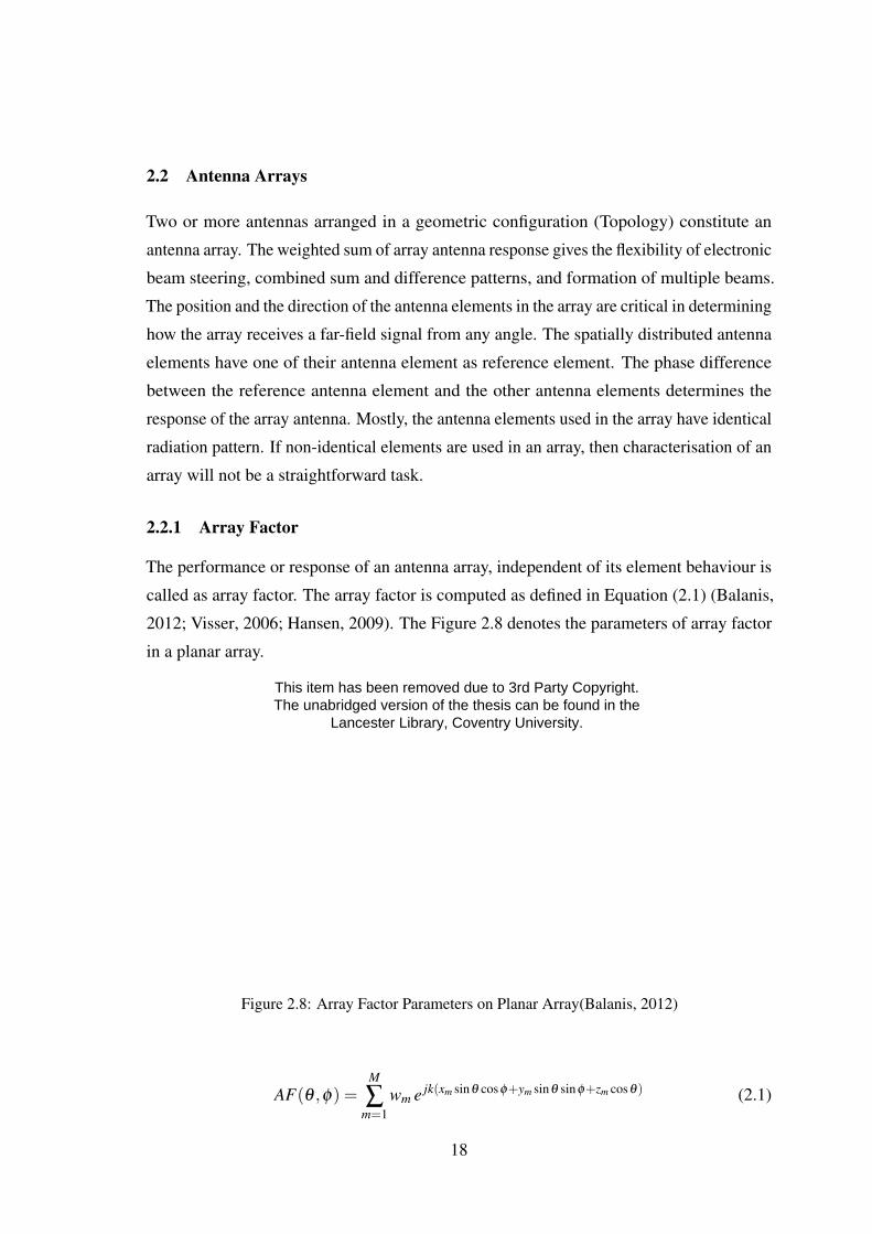
2.2 Antenna Arrays
Two or more antennas arranged in a geometric configuration (Topology) constitute an
antenna array. The weighted sum of array antenna response gives the flexibility of electronic
beam steering, combined sum and difference patterns, and formation of multiple beams.
The position and the direction of the antenna elements in the array are critical in determining
how the array receives a far-field signal from any angle. The spatially distributed antenna
elements have one of their antenna element as reference element. The phase difference
between the reference antenna element and the other antenna elements determines the
response of the array antenna. Mostly, the antenna elements used in the array have identical
radiation pattern. If non-identical elements are used in an array, then characterisation of an
array will not be a straightforward task.
2.2.1 Array Factor
The performance or response of an antenna array, independent of its element behaviour is
called as array factor. The array factor is computed as defined in Equation (2.1) (Balanis,
2012; Visser, 2006; Hansen, 2009). The Figure 2.8 denotes the parameters of array factor
in a planar array.
Figure 2.8: Array Factor Parameters on Planar Array(Balanis, 2012)
AF(θ ,φ) =M
∑m=1
wm e jk(xm sinθ cosφ+ym sinθ sinφ+zm cosθ) (2.1)
18
This item has been removed due to 3rd Party Copyright. The unabridged version of the thesis can be found in the
Lancester Library, Coventry University.

where M is the number of antenna elements;
xm,ym and zm are the co-ordinates of the mth antenna element;
k = 2π
λis the wave number, λ being wavelength;
wm is the complex weight denoting amplitude and phase of the mth antenna element.
The phase term of the array factor is only with respect to its positional coordinate of antenna
elements as well as elevation and azimuth angles (θ ,φ).
2.2.2 Pattern Multiplication
The radiation pattern of the single (individual) radiator is called element factor. The array
factor denotes the radiation pattern of the array of M isotropic radiators. The product of
element factor of the array element and array factor of the array determines the radiation
pattern of the array antenna. The above product is termed as the pattern multiplication of
the array antenna.
Array Radiation Pattern = Array Factor AF(θ ,φ) × Element Radiation Pattern (θ ,φ)
For the pattern multiplication to hold well, all antenna elements in an array have to be
mounted identically to receive or transmit the same polarization. If any of the antenna
elements are having different orientation, its polarization or propagation axis will change.
The phase term of a particular element in the array factor at angles (θ ,φ) has to match with
the individual radiation pattern of the respective element at angles (θ ,φ). Thus, factoring
the element pattern out side the array factor is not possible for dissimilar orientation of
elements. The radiation pattern of individual elements of the array has to individually
multiplied inside the array factor equation.
2.2.3 Array Manifold
The vector a(θ ,φ) which is a function of both the azimuth angle φ and elevation angle
θ in an array of M antenna elements is called the array manifold vector or array steering
vector for a corresponding direction of (θ ,φ). The response of an array antenna to a signal
with specified incidence angle, is determined by the array structure and characteristics of
antenna. The set of these steering vectors for all possible angles of incidence is defined
as antenna array manifold. The array manifold vector is measured or calculated for a
specified incident angle (J.-T. Kim, Kim, & Lee, 2013). The array manifold transforms
the change in angle of wave incidence into a change in measurement vector (Tuncer
19

& Friedlander, 2009). The change in measurement vector is correlated with (computed)
phases at the antenna terminals to steer the antenna beam towards the desired beam pointing
angle. The array manifold is two-dimensional information lying in an M-dimensional
space. The information about the positional co-ordinates and directional characteristics
of all the elements are required to calculate the array manifold. Apart from the complete
characterisation of an array, the array manifold represents the real array in M-dimensional
complex space as, (Chandran, 2005)
a(θ ,φ) =[e− jkdβ1(θ ,φ), e− jkdβ2(θ ,φ), · · · , e− jkdβM(θ ,φ)
]T(2.2)
where
βm(θ ,φ) = xm sinθ cosφ + ym sinθ sinφ + zm cosθ (2.3)
The parameter βm(θ ,φ) is the phase computation with respect to the mth antenna element
in the array along with its position coordinates.
In the case of spatial filtering or beamforming applications, the weighted sum of amplitude
and phase along with radiation pattern of the antenna element are utilized to realize the
radiation pattern of the array. In source localization and DOA estimation applications, the
data samples are collected from the antenna elements of an array and the array manifold
vector or array steering vector is employed in the estimation schemes / algorithms.
2.2.4 Effect of Antenna Element Pattern
The antenna array form cited in the array signal processing literature (Krim & Viberg,
1996; Inoue, Mori, & Arai, 2002), generally ignores the actual radiation pattern of antenna
elements. Typically, the array factor or array steering vector, in isolation of the radiation
pattern is considered for array signal processing. The radiation pattern of the antenna
element accounted through the pattern multiplication will not completely reveal the real
scenario. The use of an isotropic radiation pattern with point source as shown in Figure
2.9 is convenient for signal processing engineers to develop pattern synthesis techniques
and array signal processing algorithms. In practice, the physical dimension of the
antenna is a constraint, while utilizing the modern array algorithm. In array antenna theory,
the inter element spacing d is bounded within the limit as λ
4 ≤ d ≤ λ
2 , where λ is the
wavelength (Balanis, 2012). Figure 2.10 shows a rectangular waveguide operating in the
dominant T E10 mode with its width a = 0.75λ and height b = 0.33λ . (Here T E10 refers to
Transverse Electric wave with m = 1 and n = 0 mode (dominant mode) of the rectangular
20

Figure 2.9: Point Source Spacing
Figure 2.10: Rectangular Waveguide Element Spacing
waveguide). The minimum of inter-element spacing d shown on Figure 2.10 occurs when
the two waveguides are positioned such that the side walls of them touch each other and
the resulting d is 0.75λ which is higher than λ/2. Thus when the actual waveguide is
considered instead of approximating it by a point source, there will be a violation of the
conventional upper limit of inter-element spacing of λ/2.
2.3 Antenna Array Configurations
An antenna array is an orderly positional configuration of multiple antenna elements to
obtain desired beam characteristics. The spatial arrangement of the multiple antenna
elements and their combined radiation characteristics will lead to the narrow beam antenna.
The beam widths (HPBW and BWFN) of the antenna array shall be controlled through the
inter-element spacing, spatial arrangement and the radiation pattern of the elements.
In array signal processing, the geometric configuration of array antenna elements is very
important. The modification of antenna element and array configuration can be used to
improve angular resolution of the DOA estimation in both the azimuth and elevation angles.
The simplest antenna array configuration Uniform Linear Array (ULA) is well studied and
analysed. A ULA is capable of estimating one-dimensional (1D) DOA angle. For singly
21
This item has been removed due to 3rd Party Copyright. The
unabridged version of the thesis can be found in the Lancester Library, Coventry University.
This item has been removed due to 3rd Party Copyright. The unabridged version of the thesis can be found in
the Lancester Library, Coventry University.

polarized ULA configuration, the placement of array elements either along x-axis or y-axis
determines the DOA angles either azimuth angle φ or elevation angle θ only. For example
ULA with its elements oriented along x-axis will determine only the azimuth DOA angle
φ , since the antenna elements show spatial phase variation along the x-axis only. Likewise,
ULA with its elements oriented along y-axis will facilitate the estimation of elevation DOA
angle θ , since the antenna elements experience spatial phase variation only along y-axis.
2.3.1 One-Dimensional Array
A configuration of antenna elements arranged along a straight line with equal spacing
between the elements is called Uniform Linear Array (ULA). The simplest form of array to
realize many of the array signal processing algorithms is the ULA configuration. In a ULA
the antenna elements are geometrically arranged along only one axis (either x or y axis)
and is also called linear arrangement (Krim & Viberg, 1996; Visser, 2006; Hansen, 2009).
Figure 2.11: Uniform Linear Array
The Figure 2.11 shows the configuration of ULA. One of the antenna elements in the
ULA is considered as a reference element. Usually it will be either the first element or
the center element of the array. The signal impinging on the array will tend to have phase
difference between two successive elements, due the linear arrangement and the reception
of parallel wave fronts from far field. The received signal by the antenna elements will
have integer multiples of phase difference.
22

2.3.2 Two-Dimensional Array
The two-dimensional(2D) array configuration is the primary requirement for the estimation
of both the azimuth φ and elevation θ angles in DOA estimation. In 2D space, many
array topologies are possible to configure the antenna elements. The commonly known
two dimensional arrays are planar and circular arrangement of antenna elements. There
are also several special two dimensional configurations such as orthogonal and L shaped
configuration which are discussed in this section.
2.3.2.1 Uniform Planar Array
In the uniform planar array configuration, the antenna elements are arranged in a uniform
planar grid, thereby resembling a matrix like arrangement. A typical Uniform Planar
Array (UPA) is shown in Figure 2.12. In the UPA configuration, the antenna elements are
Figure 2.12: Uniform Planar Array Configuration
arranged over the planar grid formed over a plane and it is usually over the x−y plane such
that wave propagation direction is along the z axis only. Normally the center element of
the grid topology is chosen as the reference element to compute the phase difference of
the array elements. In Figure 2.12 the inter element spacing along the x axis and y axis
is equal, and which in turn results in a square array. The UPA configuration can also be
formed as a rectangular array with unequal number of elements oriented along the x and y
axes with uniform or non uniform inter element spacing or equal number of elements with
unequal inter element spacing.
2.3.2.2 Uniform Circular Array
In a 2D-array, the antenna elements can also be arranged in a circular fashion, such as
along the circumference of the circle. The circular array is usually configured in the x− y
23

plane and the wave propagation will be along the z axis.
Figure 2.13: Uniform Circular Array Configuration
This array is also capable of estimating both the azimuth and elevation angles of DOA.
A typical Uniform Circular Array (UCA) configuration is shown in Figure 2.13.
2.3.2.3 Cross Array
The cross array is a configuration, where the sensors or antenna elements are arranged
on two linear axes orthogonal to each other as shown in Figure 2.14. In the cross array,
the intersecting point of the orthogonally placed two linear axes may contain a common
antenna element, which will be a reference element for the array processing (Hu et al.,
2014).
24

Figure 2.14: Cross Array Configuration (Hu et al., 2014)
2.3.2.4 Orthogonal Array
The cross array can be configured in an asymmetric form which is named as orthogonal
array (N. A.-H. M. Tayem, 2005). The orthogonal array is shown in Figure 2.15.
Figure 2.15: Orthogonal Array Configuration (N. A.-H. M. Tayem, 2005)
25
This item has been removed due to 3rd Party Copyright. The unabridged version of the thesis can be found in the Lancester Library, Coventry
University.
This item has been removed due to 3rd Party Copyright. The unabridged version of the thesis can be found in the
Lancester Library, Coventry University.

The intersection of x-axis and y-axis will be at the origin of the coordinate system,
which can also be treated as a reference point. If an antenna is placed at the reference point,
the data acquired from that antenna is used as reference.
2.3.3 Three Dimensional Array
The 2D array configuration can be extended to the third dimension (3D) which is the z-axis.
The antenna elements are arranged in the three linear axes orthogonal to each other. This
configuration is shown in the Figure 2.18. In 2D and 3D configurations, where the antenna
elements are not only linearly spaced but also mutually orthogonally arranged. The array
processing can be accomplished by segmenting the array into sub-arrays. Each sub-array
is a linear array of antenna elements along its axis. The array steering vectors should be
derived based on the geometric configuration of the antenna elements. The sub-array can
be processed either independently or jointly and it depends on the algorithms used for DOA
estimation.
2.3.3.1 L-Shaped Arrays
The antenna elements can be placed along x-axis, y-axis and z-axis as well as at the
origin. Such an arrangement of antenna array has an L-shape structure. The L-Shape
arrangement extended on the third dimension which is y-axis is as shown in the Figure
2.16.(N. A.-H. M. Tayem, 2005; Liang & Liu, 2011; Harabi, Changuel, & Gharsallah,
2007)
26
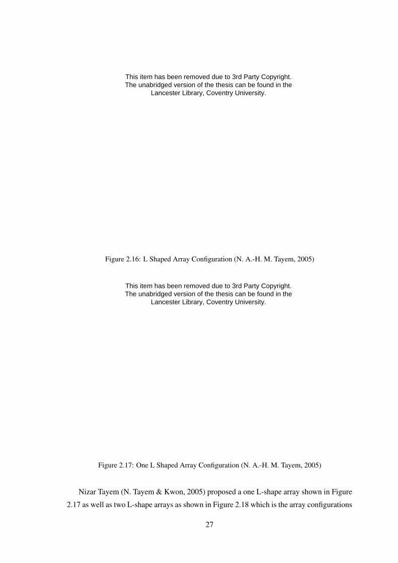
Figure 2.16: L Shaped Array Configuration (N. A.-H. M. Tayem, 2005)
Figure 2.17: One L Shaped Array Configuration (N. A.-H. M. Tayem, 2005)
Nizar Tayem (N. Tayem & Kwon, 2005) proposed a one L-shape array shown in Figure
2.17 as well as two L-shape arrays as shown in Figure 2.18 which is the array configurations
27
This item has been removed due to 3rd Party Copyright. The unabridged version of the thesis can be found in the
Lancester Library, Coventry University.
This item has been removed due to 3rd Party Copyright. The unabridged version of the thesis can be found in the
Lancester Library, Coventry University.

Figure 2.18: Two L Shaped Array Configuration (N. A.-H. M. Tayem, 2005)
for two dimensional DOA estimation without any azimuth and elevation pair matching
techniques. The authors claim that complete removal of the estimation pair matching
between azimuth and elevation angles is possible with the proposed L-shape array and
significant reduction in the RMSE of DOA estimation is also possible.
2.4 Review of DOA Estimation Algorithms
Antenna array signal processing has emerged under the broad engineering discipline of
sensor array signal processing. This active area of research involves, processing of the data
collected through antenna elements and fusing the data to perform the functions such as
DOA estimation, digital beamforming and signal enhancement.
2.4.1 Antenna Array Signal Modelling
Array signal processing deals with the extraction of information from the simultaneous
reception of data from the multiple elements of an antenna array. The estimation of
parameters is carried out through fusion of temporal and spatial information obtained via
28
This item has been removed due to 3rd Party Copyright. The unabridged version of the thesis can be found in the Lancester
Library, Coventry University.
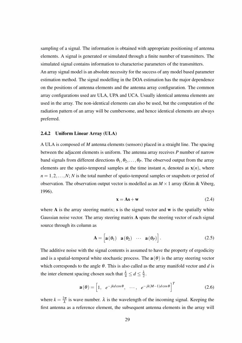
sampling of a signal. The information is obtained with appropriate positioning of antenna
elements. A signal is generated or simulated through a finite number of transmitters. The
simulated signal contains information to characterise parameters of the transmitters.
An array signal model is an absolute necessity for the success of any model based parameter
estimation method. The signal modelling in the DOA estimation has the major dependence
on the positions of antenna elements and the antenna array configuration. The common
array configurations used are ULA, UPA and UCA. Usually identical antenna elements are
used in the array. The non-identical elements can also be used, but the computation of the
radiation pattern of an array will be cumbersome, and hence identical elements are always
preferred.
2.4.2 Uniform Linear Array (ULA)
A ULA is composed of M antenna elements (sensors) placed in a straight line. The spacing
between the adjacent elements is uniform. The antenna array receives P number of narrow
band signals from different directions θ1,θ2, . . . ,θP. The observed output from the array
elements are the spatio-temporal samples at the time instant n, denoted as x(n), where
n = 1,2, . . . ,N; N is the total number of spatio-temporal samples or snapshots or period of
observation. The observation output vector is modelled as an M×1 array (Krim & Viberg,
1996).
x = As+w (2.4)
where A is the array steering matrix; s is the signal vector and w is the spatially white
Gaussian noise vector. The array steering matrix A spans the steering vector of each signal
source through its column as
A =[a(θ1) a(θ2) · · · a(θP)
]. (2.5)
The additive noise with the signal contents is assumed to have the property of ergodicity
and is a spatial-temporal white stochastic process. The a(θ) is the array steering vector
which corresponds to the angle θ . This is also called as the array manifold vector and d is
the inter element spacing chosen such that λ
4 ≤ d ≤ λ
2 .
a(θ) =[1, e− jkd cosθ , · · · , e− jk(M−1)d cosθ
]T(2.6)
where k = 2π
λis wave number. λ is the wavelength of the incoming signal. Keeping the
first antenna as a reference element, the subsequent antenna elements in the array will
29
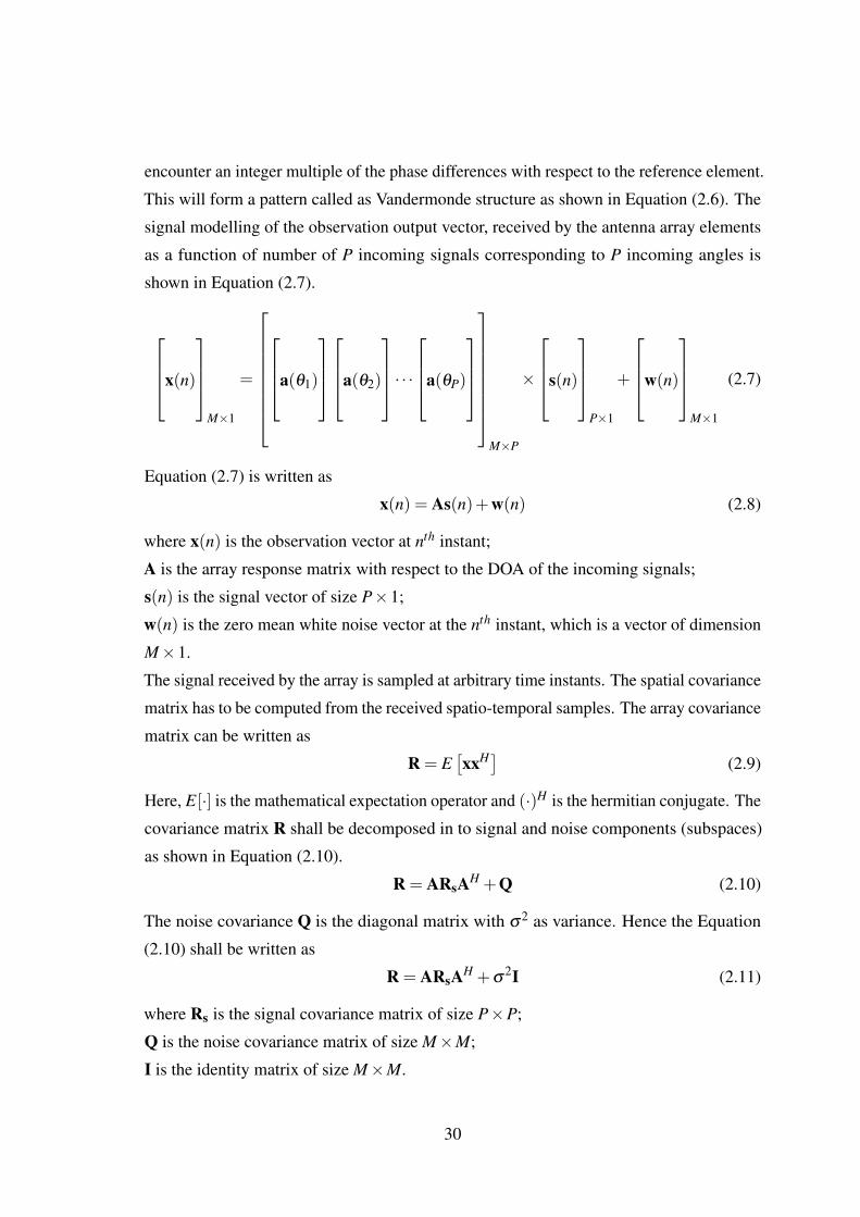
encounter an integer multiple of the phase differences with respect to the reference element.
This will form a pattern called as Vandermonde structure as shown in Equation (2.6). The
signal modelling of the observation output vector, received by the antenna array elements
as a function of number of P incoming signals corresponding to P incoming angles is
shown in Equation (2.7).
x(n)
M×1
=
a(θ1)
a(θ2)
· · ·a(θP)
M×P
×
s(n)
P×1
+
w(n)
M×1
(2.7)
Equation (2.7) is written as
x(n) = As(n)+w(n) (2.8)
where x(n) is the observation vector at nth instant;
A is the array response matrix with respect to the DOA of the incoming signals;
s(n) is the signal vector of size P×1;
w(n) is the zero mean white noise vector at the nth instant, which is a vector of dimension
M×1.
The signal received by the array is sampled at arbitrary time instants. The spatial covariance
matrix has to be computed from the received spatio-temporal samples. The array covariance
matrix can be written as
R = E[xxH] (2.9)
Here, E[·] is the mathematical expectation operator and (·)H is the hermitian conjugate. The
covariance matrix R shall be decomposed in to signal and noise components (subspaces)
as shown in Equation (2.10).
R = ARsAH +Q (2.10)
The noise covariance Q is the diagonal matrix with σ2 as variance. Hence the Equation
(2.10) shall be written as
R = ARsAH +σ2I (2.11)
where Rs is the signal covariance matrix of size P×P;
Q is the noise covariance matrix of size M×M;
I is the identity matrix of size M×M.
30
The signal covariance Rs shall be equated to the average covariance of the signal vector as
shown in Equation (2.12).
Rs = E[s(n)sH(n)
](2.12)
The covariance matrix of the observed data samples is estimated as shown in Equation
(2.13), where N is the number of data samples observed.
R =1N
N
∑n=1
x(n)xH(n) (2.13)
2.4.3 Assumptions in the DOA Estimation Schemes
The process x(n) in Equation (2.13) is a multichannel random process. The first and
second order statistics of signals and noise, characterise the above random process. An
assumption of spatial decorrelation is associated with the impinging sources. The white
noise added to the signal model is also uncorrelated with the signal sources. Coherent
sources or highly correlated sources will lead to reduction in rank of the covariance matrix.
Thus the source covariance matrix R is often presumed to be non-singular or near-singular
for highly correlated sources for the ease of computation.
In general, the distance of separation between the signal sources and antenna array is far
greater than the array dimension. This facilitates to assume that parallel wave fronts are
impinging on the array. The signals impinging on the antenna array are assumed to be
originated from the far-field distance. Thus, the signal wave fronts arriving at the antenna
array are parallel. The empirical formula for the far-field distance is 2D2/λ , where D is
the maximum dimension of the antenna and λ is the wavelength.
If the received signal has spherical wave fronts, then the signal source is said to have
originated from near-field region and the curvature of the wave front depends on the
distance between the source and the antenna array. As the distance between the source and
the antenna array becomes large, the antenna array receives the planar wave fronts (parallel
rays). Hence the source is said to be in far field region with respect to the array.
For an impinging source located at a near-field of the sensing array, the localisation of the
source is possible from the available information of relative time delays and the speed of
propagation of source. The far-field sources which impinge on the array antennas have
uniform time-delay as well as phase difference with respect to a reference antenna element.
(Krim & Viberg, 1996; N. A.-H. M. Tayem, 2005). This thesis concentrates only on
far-field source localization algorithms and approaches.
31

The multiple sources received by the antenna array are assumed to have a single carrier.
Most of the algorithms cited in the literature (Krim & Viberg, 1996) deal with the signal
model with narrow band signal sources.
The covariance matrix formed through the obtained data samples received by the antenna
arrays elements, reflects the properties of the noise in the received signal by having common
variance and de-correlation among all antennas. Such a noise is often termed as spatial
white noise. For DOA estimation, the assumption of spatial white noise is common. On the
contrary, other sources of man-made noise cannot be assumed to result in spatial white noise.
In such a case pre-whitening of noise is a must, leading to assumption of complex white
Gaussian process. The additive noise is derived from a zero mean, spatially uncorrelated
random process, which is uncorrelated (independent) with the received signal sources.
The noise has a common variance σ2 at all the array elements and is uncorrelated among
antenna elements. The analysis carried in this thesis neglects interference, atmospheric
disturbances, static and other external noise sources.
2.5 Classification of DOA Estimation Algorithms
In general the DOA estimation algorithms can be broadly classified into two types
• Beamforming based estimation technique
• Subspace based estimation technique
2.5.1 Beamforming Based DOA Estimation Techniques
Beamforming is a technique which focuses Electromagnetic (EM) radiation in a particular
direction. The antenna array essentially combines the effects of many antenna elements
to form one or more beams. It is developed as a technique that could accurately direct or
position a beam in free space. The formation of array and combinational effects permit
the development of antennas of narrow beam-widths with high gain. The pointed or
focussed beam will be used to scan the surrounding angular region. The weight and sum
techniques are used to scan the angular region. In the process of scanning, the angle which
maximizes the power of the received signal will be identified as the estimated DOA of
the incoming signal. Bartlett’s conventional beamforming or delay and sum beamformer
(Bartlett, 1950) and Capon’s minimum variance technique (Capon, 1969) are the classical
beamforming techniques. The beamforming based techniques are formulated as spatial
32
filtering approaches to estimate the DOA. In these techniques, the main lobe of the antenna
is used to scan the entire region of interest. The direction which maximizes the received
signal power is determined as the DOA.
2.5.1.1 Bartlett’s Conventional Beamformer
The conventional (Bartlett) beamformer (Bartlett, 1950) is a Fourier-based spectral analysis
of spatio-temporal sampled data. This technique is also named as the delay and sum
beamformer. As the name indicates Delay and Sum, complex weights will be applied to the
received signal by the array elements and summed to obtain the output of the beamformer.
The complex weights introduce the phase in the antenna elements which steers the pointing
angle of antenna main lobe. This inturn suppresses the unwanted interference signal from
other directions. The scan angle, which yields the maximum power of the received signal
is determined as the DOA of the signal. This technique attempts to maximize the expected
output power as stated in expression (2.14) by applying optimal weights to the signals
received by the array elements, and thus improves the SNR of the signal (Van Veen &
Buckley, 1988)
maxw s.t wHw=1
E[wHx(n)xH(n)w]. (2.14)
The optimal weight wopt is computed such that, it is parallel to the a(θ) as shown in
Equation (2.15). Here a(θ) is the steering vector for the DOA angle θ and aH(θ) is the
Hermitian conjugate of the array steering vector.
wopt =a(θ)√
aH(θ)a(θ)(2.15)
The angular spectrum PB(θ) for Bartlett’s method is computed through the function given
in Equation (2.16) for all the angles of θ (Krim & Viberg, 1996)
PB(θ) =aH(θ)Ra(θ)aH(θ)a(θ)
(2.16)
The covariance matrix R is estimated from the samples received by the elements of antenna
arrays. The DOA estimate is obtained by the highest peaks of the angular spectrum of
the function of Equation (2.16). The beamformers developed invoking spatial-filtering
were valid only for narrowband signals implying their characterisation only through a
single frequency. This approach also suffers from fundamental limitation due to the beam
width of the array elements. Its performance depends only on the physical size of the array
(aperture). Further, the associated data collection time and Signal-to-Noise Ratio (SNR)
have little significance (Bartlett, 1950; Coldrey & Viberg, 2006).
33
2.5.1.2 Capon’s MVDR Algorithm
The limitation of the conventional beamformer is that, for the detection of multiple sources,
the angular separation between the sources must be greater than the beamwidth of the array.
This limitation is overcome by Capon’s approach of Minimum Variance Distorsionless
Response (MVDR). Bartlett’s conventional beamformer uses every available degree of
freedom to concentrate the received energy along one direction, namelythebearing angle
of interest. This has been overcome by the minimization constraints of Capon’s approach.
Capons approach interprets minimization constraints as a sacrifice in the noise suppression
capability to obtain more focused nulling in the directions other than the DOA sources
present. Thus spectral leakage from closely spaced sources is reduced. The resolution
capability of the Capon beamformer is dependent on the array aperture and the SNR (Krim
& Viberg, 1996). The received samples have the mixed signal power of the desired DOA
of the source as well as the undesired sources. This method attempts to minimize the
signal of the undesired DOA sources, but keeping the gain of the desired sources fixed as a
constraint. This constrained minimization results in a weight vector called as Minimum
Variance Distortionless Response (MVDR). The weight vector wc for the Capon’s MVDR
approach after the constrained optimization is given in Equation (2.17).
wc =Ra(θ)
aH(θ)Ra(θ)(2.17)
The angular spectrum PC(θ) for computing DOA using Capon’s method after applying the
constraints is given by Equation (2.18)(Krim & Viberg, 1996).
PC(θ) =1
aH(θ)R−1a(θ)(2.18)
The Capon’s method yields better response, compared to conventional beamformer in terms
of sharpness of the peak estimation. It has higher complexity because it involves matrix
inversion which is an intensive computation O(N3). It suffers when the correlated sources
impinge on the array. The emergence of parameter estimation approach offers inspirations
for the subsequent efforts in Maximum Entropy (ME) spectral estimation method and the
initial applications of Maximum Likelihood (ML) principle (Hayes, 2009).
2.5.2 Subspace Based Estimation Techniques
The new age of high-resolution computations of DOA commenced with the subspace based
estimation techniques. The class of algorithms known as subspace based techniques was
34

introduced in the mid 1970s and was a revolution in the field of high-end and computa-
tionally intensive estimation algorithms. The estimation is purely based on the underlying
data model. This algorithm decomposes the vectors spanned by the correlation matrix
into signal subspace and noise subspace. The significant aspect of these techniques is that
the decomposed signal subspace and noise subspace vectors are orthogonal to each other.
The orthogonality property is used for the search based estimation, polynomial rooting
based estimation as well as least squares based estimation. The results of subspace based
methods are much more promising in terms of accuracy and angular resolution of DOA
when compared to other techniques such as Bartletts and Capon’s method. The MUSIC and
ESPRIT are the classical subspace based DOA estimation algorithms. The array aperture
does not limit the resolution capability of subspace techniques.
The array covariance matrix R of the observed signal vector is given as
R = E[xxH]= ARsAH +Q (2.19)
where x is the observed signal vector from the antenna array;
E(.) is the expectation operator to make sample covariance matrix as shown in Equation
(2.13);
(.)H is the Hermitian transpose;
A is the array steering matrix as defined in Equation(2.5);
Rs is the signal covariance matrix;
Q is the noise covariance matrix. Assuming the number of sources P is known, the
estimated source angles are calculated with respect to the reference element of the array
as θ1,θ2, · · · ,θP. The covariance matrix R is decomposed using eigen decomposition and
shall be written using eigenvalues and eigenvectors as
R =M
∑i=1
λivivHi = VΛVH (2.20)
where, λ is the eigenvalue and v is the eigenvector. The eigenvalues are sorted in descending
order such as λ1 ≥ λ2 ≥ ·· · ≥ λP. The respective eigenvectors form the columns of the
matrix V as shown in Equation (2.21).
V =
v1
v2
· · ·vP
vP+1
· · ·vM
(2.21)
35

The eigenvalues will be arranged as diagonal elements of the matrix Λ as shown in Equation
(2.22).
Λ =
λ1 0 · · · · · · 0
0 λ2...
... . . .
λP
λP+1...
... ¨ 0
0 0 · · · · · · 0 λM
(2.22)
The sum of eigenvalues λi, for i > P is equal to the variance of the noise present in the data
covariance matrix, stated in Equation (2.23).
λP+1 +λP+2 + · · ·+λM = σ2 (2.23)
The eigenvectors vi for i > P satisfy the condition as shown in Equation (2.24).
Rvi = λivi = σ2vi (2.24)
Rvi =(
ARsAH +σ2I)
vi (2.25)
(ARsAH
)vi = 0 (2.26)
By the full rank property, A and Rs in Equation (2.26) will be
vHi A = 0 (2.27)
where i > P
G = SS+NS (2.28)
SS is the signal subspace and NS is the noise subspace which are described in Equations
(2.29) and (2.30) and G is the sum of signal and noise subspace.
SS = span[a(θ1) , a(θ2) , · · · , a(θP)
](2.29)
NS = span[vP+1, vP+2, · · · , vM
]. (2.30)
36

The mathematical steps or procedures describing in this section for the computation of
covariance matrix and the decomposition of signal and noise subspace are applicable to
both Pisarenko and MUSIC algorithms. Therefore the steps will not be repeated in the
subsequent subsections.
2.5.2.1 Pisarenko Harmonic Decomposition
The Pisarenko method (Pisarenko, 1973) of parameter estimation was originally developed
for the spectral estimation problems. This method acted as a base for the revolutionary
emergence of the subspace based algorithms. This method assumes that a signal is com-
posed of a finite number of complex exponentials in the presence of white noise. A priori
knowledge of the number of complex exponential P present in the signal, is used to form
the covariance matrix of size (P+1)× (P+1). The number of complex exponentials also
refers to number of sources. The number of array elements M used in the case of Pisarenko
method is one more than the number of sources, M = P+1. The covariance matrix of size
M×M is decomposed into signal and noise subspace matrices. The signal subspace and
the noise subspace are orthogonal to each other. The dimension of the noise subspace is
always one and it is spanned by the eigenvectors corresponding to the least eigenvalue
(Pisarenko, 1973; Hayes, 2009).
PPHD (θ) =1
|vHmina(θ) |2
(2.31)
The angular spectrum PPHD (θ) estimation using Pisarenko harmonic decomposition is
stated in Equation (2.31), in which vmin is the eigenvector corresponding to minimum
eigenvalue, and a(θ) is the array steering vector.
2.5.2.2 MUSIC Algorithm
The MUSIC Algorithm (Schmidt, 1986) is a classical high resolution subspace based
algorithm to estimate the DOA of the signal sources. This algorithm is based on the property
that the desired array signal response is orthogonal to the noise subspace. The orthogonality
implies that the estimated autocorrelation matrix is decomposed (de-correlated) into the
signal and noise subspaces (eigenvectors). The block diagram describing the computation
flow of the MUSIC algorithm is shown in Figure 2.19. In a correlated environment some of
the signal eigenvectors may diverge into noise eigenvectors, which in turn tends to degrade
37
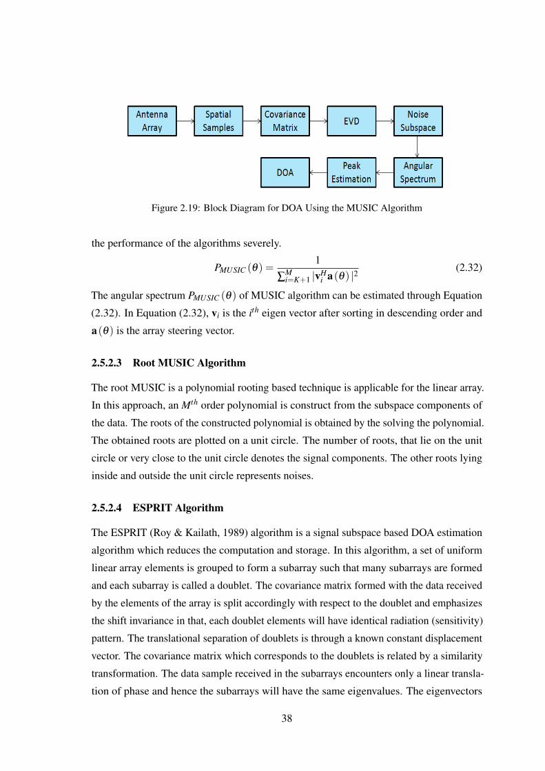
Figure 2.19: Block Diagram for DOA Using the MUSIC Algorithm
the performance of the algorithms severely.
PMUSIC (θ) =1
∑Mi=K+1 |vH
i a(θ) |2(2.32)
The angular spectrum PMUSIC (θ) of MUSIC algorithm can be estimated through Equation
(2.32). In Equation (2.32), vi is the ith eigen vector after sorting in descending order and
a(θ) is the array steering vector.
2.5.2.3 Root MUSIC Algorithm
The root MUSIC is a polynomial rooting based technique is applicable for the linear array.
In this approach, an Mth order polynomial is construct from the subspace components of
the data. The roots of the constructed polynomial is obtained by the solving the polynomial.
The obtained roots are plotted on a unit circle. The number of roots, that lie on the unit
circle or very close to the unit circle denotes the signal components. The other roots lying
inside and outside the unit circle represents noises.
2.5.2.4 ESPRIT Algorithm
The ESPRIT (Roy & Kailath, 1989) algorithm is a signal subspace based DOA estimation
algorithm which reduces the computation and storage. In this algorithm, a set of uniform
linear array elements is grouped to form a subarray such that many subarrays are formed
and each subarray is called a doublet. The covariance matrix formed with the data received
by the elements of the array is split accordingly with respect to the doublet and emphasizes
the shift invariance in that, each doublet elements will have identical radiation (sensitivity)
pattern. The translational separation of doublets is through a known constant displacement
vector. The covariance matrix which corresponds to the doublets is related by a similarity
transformation. The data sample received in the subarrays encounters only a linear transla-
tion of phase and hence the subarrays will have the same eigenvalues. The eigenvectors
38
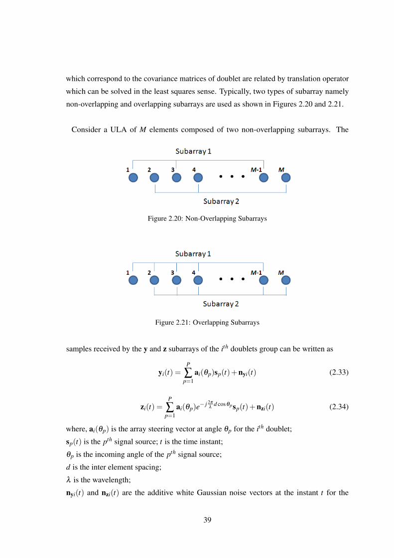
which correspond to the covariance matrices of doublet are related by translation operator
which can be solved in the least squares sense. Typically, two types of subarray namely
non-overlapping and overlapping subarrays are used as shown in Figures 2.20 and 2.21.
Consider a ULA of M elements composed of two non-overlapping subarrays. The
Figure 2.20: Non-Overlapping Subarrays
Figure 2.21: Overlapping Subarrays
samples received by the y and z subarrays of the ith doublets group can be written as
yi(t) =P
∑p=1
ai(θp)sp(t)+nyi(t) (2.33)
zi(t) =P
∑p=1
ai(θp)e− j 2π
λd cosθpsp(t)+nzi(t) (2.34)
where, ai(θp) is the array steering vector at angle θp for the ith doublet;
sp(t) is the pth signal source; t is the time instant;
θp is the incoming angle of the pth signal source;
d is the inter element spacing;
λ is the wavelength;
nyi(t) and nzi(t) are the additive white Gaussian noise vectors at the instant t for the
39
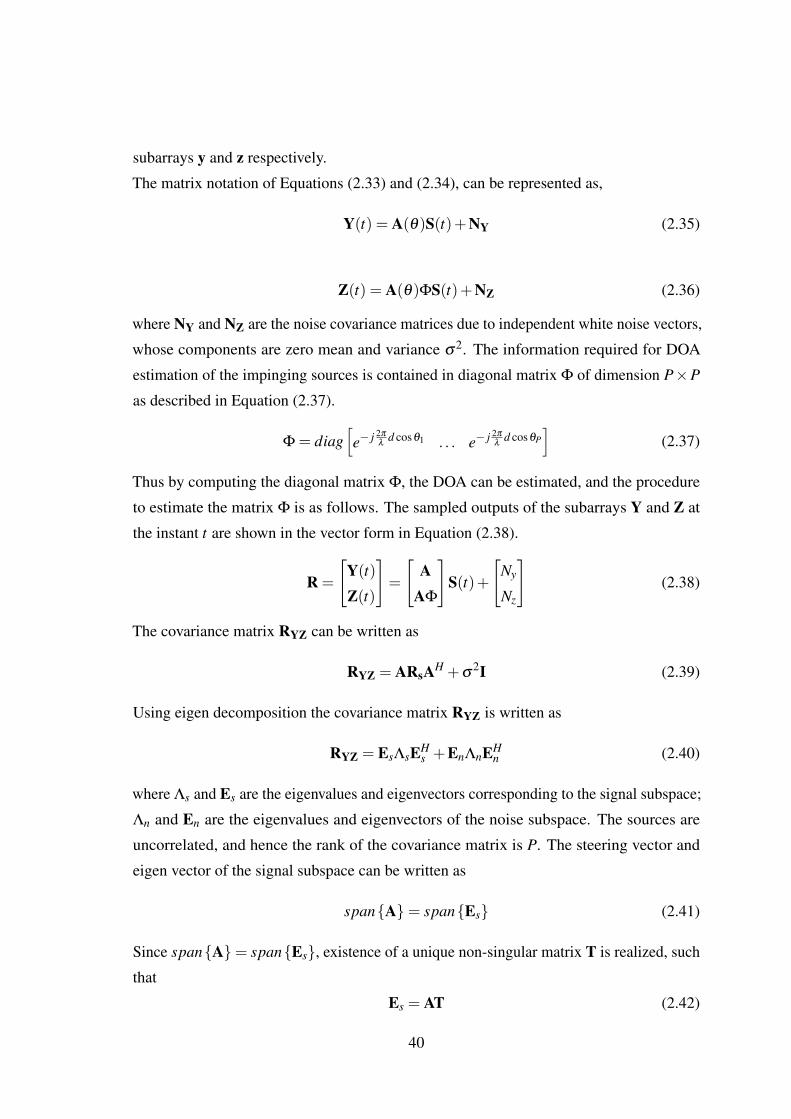
subarrays y and z respectively.
The matrix notation of Equations (2.33) and (2.34), can be represented as,
Y(t) = A(θ)S(t)+NY (2.35)
Z(t) = A(θ)ΦS(t)+NZ (2.36)
where NY and NZ are the noise covariance matrices due to independent white noise vectors,
whose components are zero mean and variance σ2. The information required for DOA
estimation of the impinging sources is contained in diagonal matrix Φ of dimension P×P
as described in Equation (2.37).
Φ = diag[e− j 2π
λd cosθ1 . . . e− j 2π
λd cosθP
](2.37)
Thus by computing the diagonal matrix Φ, the DOA can be estimated, and the procedure
to estimate the matrix Φ is as follows. The sampled outputs of the subarrays Y and Z at
the instant t are shown in the vector form in Equation (2.38).
R =
[Y(t)
Z(t)
]=
[A
AΦ
]S(t)+
[Ny
Nz
](2.38)
The covariance matrix RYZ can be written as
RYZ = ARsAH +σ2I (2.39)
Using eigen decomposition the covariance matrix RYZ is written as
RYZ = EsΛsEHs +EnΛnEH
n (2.40)
where Λs and Es are the eigenvalues and eigenvectors corresponding to the signal subspace;
Λn and En are the eigenvalues and eigenvectors of the noise subspace. The sources are
uncorrelated, and hence the rank of the covariance matrix is P. The steering vector and
eigen vector of the signal subspace can be written as
span{A}= span{Es} (2.41)
Since span{A}= span{Es}, existence of a unique non-singular matrix T is realized, such
that
Es = AT (2.42)
40

The signal subspace Es shall be partitioned according to the samples of subarrays Y and Zformulated in the vector form shown in Equation (2.43).
Es =
[EY
EZ
]=
[AT
AΦT
](2.43)
The signal subspaces EY and EZ can also be stacked column wise as shown Equation
(2.44).
EsYZ =[EY EZ
](2.44)
Since the rank of EsYZ is also P, it implies the existence of matrix F⊂ C2P×P with rank P
such that,
0 =[EY EZ
]F = EYFY +EZFZ (2.45)
ATFY +AΦTFZ = 0 (2.46)
Here, F spans the null space of EsYZ. A matrix Ψ of size P×P is defined as
Ψ =−FYF−1Z (2.47)
Equation (2.45) can be written as
ATΨT−1 = AΦ (2.48)
The implication of matrix A having full rank property, yields
TΨT−1 = Φ (2.49)
Equation (2.49) can be rearranged to compute matrix Ψ as
Ψ = T−1ΦT (2.50)
The eigenvalues of Ψ are equal to the diagonal elements of Φ. The matrix T spans its
column space with the eigenvectors of Ψ. This property leads to the development of
ESPRIT algorithm.
The ESPRIT algorithm is also known as SUbspace Rotation Estimation (SURE). The
accuracy of the MUSIC and ESPRIT techniques increases as M increases. In case of
temporal data processing for frequency estimation, M refers to the temporal window size.
In array signal processing, M denotes the number of sensors or antennas. However in
41

practical application, M cannot be very large. Both MUSIC and ESPRIT algorithms
utilize eigen decomposition and the parameter M has the computational complexity of
O(M3). M is fixed such that M � N. It is cited in (Stoica & Soderstrom, 1991), that
the ESPRIT algorithm is preferred for its higher accuracy when compared to MUSIC
algorithm for the case of temporal data processing. In case of the array signal processing,
MUSIC algorithm is preferred over ESPRIT, due to processing of higher number samples.
Generally, the ESPRIT algorithm is not required to search for all steering vectors as in the
MUSIC algorithm. Hence its computational efficiency is more compared to the MUSIC
algorithm. However, the ESPRIT algorithm is limited to operate with ULA geometries due
to its rotational invariance property whereas, the MUSIC algorithm can be used with any
arbitrary array configurations.
2.5.2.5 Other Methods
The de-correlation of the signal and noise eigenvectors has a critical role in the achievable
resolution of the DOA estimators. Many attempts have been made in the past to improve
the de-correlation between the signal and noise subspaces. Spatial Smoothing MUSIC
(SS-MUSIC) and Signal Subspace-Scaled MUSIC (SSS-MUSIC) are some of the methods
already available for improving the resolution. The above subspace based techniques are
primarily signal processing based approach for improving the de-correlation (Shan, Wax,
& Kailath, 1985; S.-W. Chen, Jen, & Chang, 2009).
The Matrix Pencil (MP) method utilizes the spatial samples received by the antenna array.
In this method, individual snapshot (sample) based analysis is carried out to take care
of non-stationary environments to facilitate ease of handling. The MP method does not
require spatial smoothing for the DOA estimation in a multipath coherent environment.
The reduction in computational complexity of covariance matrix is accomplished by the
conversion of complex matrix to real matrix and its eigenvectors by a unitary transformation
matrix. The transform matrix maps centro-Hermitian matrices to real matrices (Yilmazer,
Koh, & Sarkar, 2006).
The subspace based Propagator Method (PM) is devoid of EVD or SVD of the Cross-
Spectral Matrix (CSM) of the received signals. This method was perceived as a possible
alternative to the MUSIC algorithm. The computational load is significantly smaller than
the classical subspace based MUSIC and ESPRIT algorithms. The steering vectors of the
array enable the extraction of the propagator (a linear operator) from the received data
42
(Marcos, Marsal, & Benidir, 1995).
2.6 Antenna Elements and Array Configuration for DOA Estimation
The several decades of research in array signal processing has been oriented towards
the improvement of the estimation techniques and algorithms. However the emphasis
of research towards the antenna array element and array configuration is rather limited.
The geometry of the sensor array configuration has significant effects on the performance
of DOA estimation algorithms. Research papers orient the estimation techniques with
respect to the classical ULA, UCA and UPA configurations, because of their simplicity in
implementation and straight forwardness. Some special configurations such cross array,
L-type array have also been addressed for the two dimensional DOA estimation.
Most of the cited techniques and algorithms for DOA estimation (Krim & Viberg, 1996)
assume the isotropic elements with omni-directional radiation pattern as element pattern
for the antenna array element. Under the realistic scenario, this assumption is not valid.
The antenna element designed for RF and Microwave frequencies are not omni-directional
in practice. The assumption of identical antenna elemental characteristics is considered as
fair one. The radiation pattern of the antenna elements of the array has significant impact
on the DOA performance of estimation approaches.
The mutual coupling effect of the antenna elements in the array has interfering effects in
the received signal, which may tend to degrade the performance of the estimation tech-
niques. Formulation or analysis of approach to minimize the mutual coupling effect, which
indirectly improves the DOA estimation has not been widely addressed in the literature.
Initially, the large number of antenna elements in an array was used to produce the narrow
pencil beam to detect and estimate the DOA of sources. The beamforming based methods
are utilized in these approaches. After the arrival of subspace based techniques, lesser
number of antenna elements are utilized to take advantage of the DOA estimation algorithm
with higher resolution. Recently, research towards smaller antenna array to achieve high
resolution DOA estimation has emerged.
The consequence of reduction in number of antenna elements will eventually will lead to
lesser number of samples to be processed for DOA estimation. Therefore subspace based
technique is getting prominence for high resolution DOA estimation.
It has been identified that, the polarization of the antenna is a factor to improve the DOA
estimation schemes. In this regard, diversely polarized antenna elements have the potential
43

to improve the DOA estimation schemes. A mutually orthogonal arrangement of dipoles
Figure 2.22: Mutually Orthogonal Arrangement of Dipoles (Chick et al., 2011)
and biconical antennas are proposed for DFS (Chick et al., 2011). In this paper, three
biconical antennas with same angular cone are co-located. Thus the incident wave front
rely only on the polarization of antenna. This mutually orthogonal arrangement cannot
detect the phase delay between the antenna elements, since it is co-located. The mutually
Figure 2.23: Mutually Orthogonal Arrangement of Antennas (Chick et al., 2011)
orthogonal arrangement of biconical antennas is shown in Figure 2.23. The computation of
the vector which is perpendicular to the locus of the instantaneous electric field vector is
utilized in this array configuration. The typical ML and MUSIC algorithms are used for
DOA estimation.
A 3-axis orthogonal array antenna is proposed by Kim et al. (M. Kim et al., 2004) to
determine the direction of the RFID tag. Three loop antennas of the same geometry and
characteristics are arranged in 3-axis to form orthogonal array antenna as shown in Figure
2.24. The comparison of measured signal strength in each axis of the antenna yields the
44
This item has been removed due to 3rd Party Copyright. The unabridged version of the thesis can be found in
the Lancester Library, Coventry University.
This item has been removed due to 3rd Party Copyright. The
unabridged version of the thesis can be found in the
Lancester Library, Coventry University.

direction information. Also the distance is estimated by phase shift obtained in each of the
antenna.
Figure 2.24: 3 Axis Orthogonal Antenna (M. Kim et al., 2004)
A patch antenna array with polarization discrimination is proposed by Yoshimura
et al. in (Yoshimura et al., 2011). A 12 element antenna array with linear polarization
discrimination circuit made up of diodes is proposed as shown in Figure 2.25.
45
This item has been removed due to 3rd Party Copyright. The unabridged version of the thesis can be found in the Lancester Library, Coventry
University.
Figure 2.25: 12-Element Array Antenna for Orthogonal Polarization Discrimination (Yoshimura et
al., 2011)
The received signals by the array 1 and array 2 are multiplied at the discriminating
circuit and the multiplier output voltage corresponding to the polarization angle is obtained.
Consequently, the received polarization angle is discriminated by the polarity of the output
voltage of the multiplier. The direction of the fields is shown in Figure 2.26.
46
This item has been removed due to 3rd Party Copyright. The unabridged version of the thesis can be found in the Lancester Library, Coventry University.
Figure 2.26: Antenna Array Behaviour with Schematic Current Distributions (Yoshimura et al.,
2011)
This antenna array can be utilized for dual linear polarization discrimination with very
good cross polarization suppression. Simultaneous reception of both the horizontal and
vertical polarized components cannot be achieved with this configuration. Wei and Guo
(Wei & Guo, 2014) proposed a signal covariance technique with pair matching for 2D DOA
estimation using the L-shaped array configuration of Figure 2.16. In this technique, two
signal covariance matrices for each of the subarray are formed and a permutation matrix is
formed for optimal matching of DOAs estimated through 1D subarrays. A technique for
estimation of DOA using the Cross Covariance Matrix (CCM) realized through two arrays
namely ULA and Sparse Linear Array (SLA) has been proposed by Gu et al. (Gu, Zhu, &
Swamy, 2015).
2.7 DOA Tracking of Non Stationary Signal Sources
The classical high resolution DOA estimation techniques like MUSIC and ESPRIT ad-
dressed in (Schmidt, 1986; Roy & Kailath, 1989) are based on the eigen decomposition.
These algorithms are associated with higher computational complexity because of the
numerical techniques involved in the computation of eigenvectors for the sample covari-
ance matrix. The major computation of algorithms is devoted to the decomposition of
subspace itself. The subspace based robust DOA estimation algorithm without the direct
47
This item has been removed due to 3rd Party Copyright. The unabridged version of the thesis can be found in the Lancester Library, Coventry University.

EVD computation is not adequately addressed in the published literature.
For the case of non-stationary sources, tracking DOA is essential for certain applications
such as mobile communications. The computational complexity is increased by N folds,
N refers to number of spatio temporal samples of the wave incident on the array. Due to
time and space variation of the impinging signal characteristics, it is essential to estimate
DOA for every sampling instant for higher accuracy. However, a single snapshot of the
received sample, associated with noise cannot reveal the exact parameter of interest in the
computation. It is preferred to utilize the past received samples of the impinging signal
sources despite time and space variations present in it. The moving average and weighted
average over the past received samples, tend to estimate the DOA more accurately when
compared to the estimation through the instant samples alone. Processing of every new
sample received along with the past sample increases computational complexity and time.
As stated earlier, computing EVD or SVD alone occupies a significant computation load in
the algorithm.
2.7.1 Singular Value Decomposition (SVD)
SVD decomposes the covariance matrix into left-hand and right-hand matrices. A descrip-
tive diagonal matrix consisting of singular values, separates the two matrices. The SVD
technique is utilized for the case of singular matrices or numerically very close to singular.
Given a matrix A of order M×N, where M > N, can be decomposed as shown in Equation
(2.51).
A = UΣVT (2.51)
A
M×N
=
U
M×N
σ1
. . .
σM
M×N
V
T
M×N
(2.52)
The decomposition of matrix A is a product of M×N column orthogonal matrix U, an
N×N diagonal matrix Σ with positive or zero elements and the transpose of an N×N
orthogonal matrix V. The diagonal elements of matrix Σ are also called singular values.
Also matrices U and V have their column span the left and right singular vectors of
the matrix A. The left and right singular vectors have similar properties of the eigen
vectors. Mostly these singular vectors and eigenvectors are interchangeably used in the
subspace algorithm. The computation of eigenvectors or singular vectors through the
48

classical approach like Jacobi or Power iteration methods involve higher computational
complexities. The computation time is directly proportional to the order of the matrix
under decomposition. The adaptive systems, uses this SVD technique for the reduction of
computation resources (Vershinin, 2014).
2.7.2 Subspace Tracking Algorithms
The subspace tracking algorithms are more efficient than conventional SVD techniques
to update the subspace components of the vector sequence. Initially, Karasalo proposed a
method of signal subspace averaging in a least squares sense (Karasalo, 1986). Later the
subspace tracking progressed from the exploitation of classical eigen structure techniques
such as QR algorithm, Jacobi rotation, power iteration, and Lanczos method (Comon
& Golub, 1990). The subspace tracking algorithms like BiSVD (Strobach, 1997), BiLS
(Ouyang & Hua, 2005) are used for sequential updating of the subspace components.
The Projection Approximation Subspace Tracking (PAST) (B. Yang, 1995) attempts for
solution to an exponentially weighted least square of the data matrix using unconstrained
minimization. Based on well known Recursive Least Square (RLS) method, the signal
subspace components are tracked efficiently. The obtained signal subspaces are not exactly
orthonormal, which is a limitation of the PAST algorithm. Later the PAST algorithm
is improved with orthonormal subspace components developed as Orthonormal PAST
(OPAST) algorithm by (Abed-Meraim, Chkeif, & Hua, 2000). Estimation and tracking
of DOA taking into account the mutual coupling between the elements of ULA has
been proposed by Liao et al. (Liao, Zhang, & Chan, 2012). Liao et al. propose the
joint estimation of DOAs and mutual coupling matrix by invoking the subspace tracking
techniques such as Modified PAST (MPAST) and OPAST for slow varying subspace
components. For the case of rapid changing subspace components, they propose Kalman
Filter with variable number of measurements (KFVM). In the analysis of Liao et al., for
higher number of samples, the term subspace leakage refers to the deviation of the sample
covariance matrix from the true covariance matrix. The solution to the problem of subspace
leakage has been addressed in (Shaghaghi & Vorobyov, 2015) through a root-swap method
in the root MUSIC algorithm.
49

2.8 DOA Estimation of Wideband Signals
The signal with its energy spread over a broad range of frequencies is in general termed
as wide-band or broad band signal. Initial attempts in the DOA estimation algorithms
were directed only towards the narrowband signal sources, but many applications such as
wireless communications warrant the localization of the wideband signal sources. The
DOA estimation of wide-band signal sources has been attempted by many researchers in
the past.
Figure 2.27: Narrowband and Wideband Signal Sources
Many concepts of DOA estimation in the narrow band case can be extended to the
wideband situation. The design of a wideband beamformer involves a subband decomposi-
tion and subsequent design of beamformer for subband (narrow band) frequencies. This
implies an application of spatio temporal filter to the samples received by the array. Hence
such an array is often termed as filter and sum structure. Therefore the determination of the
coefficients of the spatio-temporal filters constitutes the main task of the wideband beam-
former. The narrow band and wideband sources are generated and its discrete frequency
spectrum is shown the Figure 2.27. In a typical scenario, the narrow band signal appears as
a spike at the corresponding frequency, where as the wideband signal spreads over the band
50
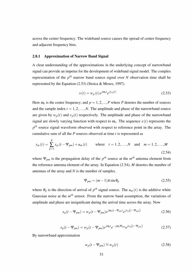
across the center frequency. The wideband source causes the spread of center frequency
and adjacent frequency bins.
2.8.1 Approximation of Narrow Band Signal
A clear understanding of the approximations in the underlying concept of narrowband
signal can provide an impetus for the development of wideband signal model. The complex
representation of the pth narrow band source signal over N observation time shall be
represented by the Equation (2.53) (Stoica & Moses, 1997).
x(t) = wp (t)e jωote jvp(t) (2.53)
Here ωo is the center frequency; and p = 1,2, ...,P where P denotes the number of sources
and the sample index t = 1,2, . . . ,N. The amplitude and phase of the narrowband source
are given by wp(t) and vp(t) respectively. The amplitude and phase of the narrowband
signal are slowly varying function with respect to ωo. The sequence x(t) represents the
pth source signal waveform observed with respect to reference point in the array. The
cumulative sum of all the P sources observed at time t is represented as
ym (t) =P
∑p=1
xp (t−Ψpm)+um (t) where t = 1,2, . . . ,N and m = 1,2, . . . ,M
(2.54)
where Ψpm is the propagation delay of the pth source at the mth antenna element from
the reference antenna element of the array. In Equation (2.54), M denotes the number of
antennas of the array and N is the number of samples.
Ψpm = (m−1)π sinθp (2.55)
where θp is the direction of arrival of pth signal source. The um (t) is the additive white
Gaussian noise at the mth sensor. From the narrow band assumption, the variations of
amplitude and phase are insignificant during the arrival time across the array. Now
xp(t−Ψpm) = wp(t−Ψpm)e jωo(t−Ψpm)e jvp(t−Ψpm) (2.56)
xp(t−Ψpm) = wp(t−Ψpm)e jωote− jωoΨpme jvp(t−Ψpm) (2.57)
By narrowband approximation
wp(t−Ψpm)∼= wp(t) (2.58)
51

and
vp(t−Ψpm)∼= vp(t) (2.59)
xp(t−Ψpm)∼= xp(t)e jωoΨpm (2.60)
This implies that the time delay is transformed into only a phase delay. The center frequency,
the inter element spacing and DOA determine this phase delay. However, it is independent
of the time variable.
2.8.2 Wideband Signal Model for Linear Array
For the case where P number of far-field point sources are observed by M sensors arranged
in a linear array geometry with additive white Gaussian noise, the spectral output of the
array of the wideband sources for (narrowband) frequency f and time sample t is given by
the Equations (2.61) and (2.62).
x( f , t) = A( f ,θ)s( f , t)+n(t) (2.61)
=P
∑p=1
a( f ,θp)sp( f , t)+n( f , t) (2.62)
where the signal source is a vector s( f , t) represented as[s1( f , t), s2( f , t), . . . ,sP( f , t)
]T.
The DOA (bearing) angle vector of the P sources is denoted as vector θ =[θ1, θ2, . . . ,θP
].
The array manifold matrix of size M×P shall be defined as
A( f ,θ) =[a( f ,θ1), a( f ,θ2), . . . ,a( f ,θP)
]with a( f ,θp) the array steering vector for
the pth source at frequency f and n( f , t) is the noise vector that is spectrally and spatially
uncorrelated. The noise is also uncorrelated with the source signals.
The structure of the steering vector, a( f ,θ) changes significantly with the geometry of the
array, since the steering vector establishes the relative phasing across the array to respond
to source at a specific angle. For a ULA with M elements with spacing d between them,
the steering vector takes the form
a( f ,θ) =
1
e j 2π fc d sinθ
e j 2π fc 2d sinθ
...
e j 2π fc (M−1)d sinθ
(2.63)
52
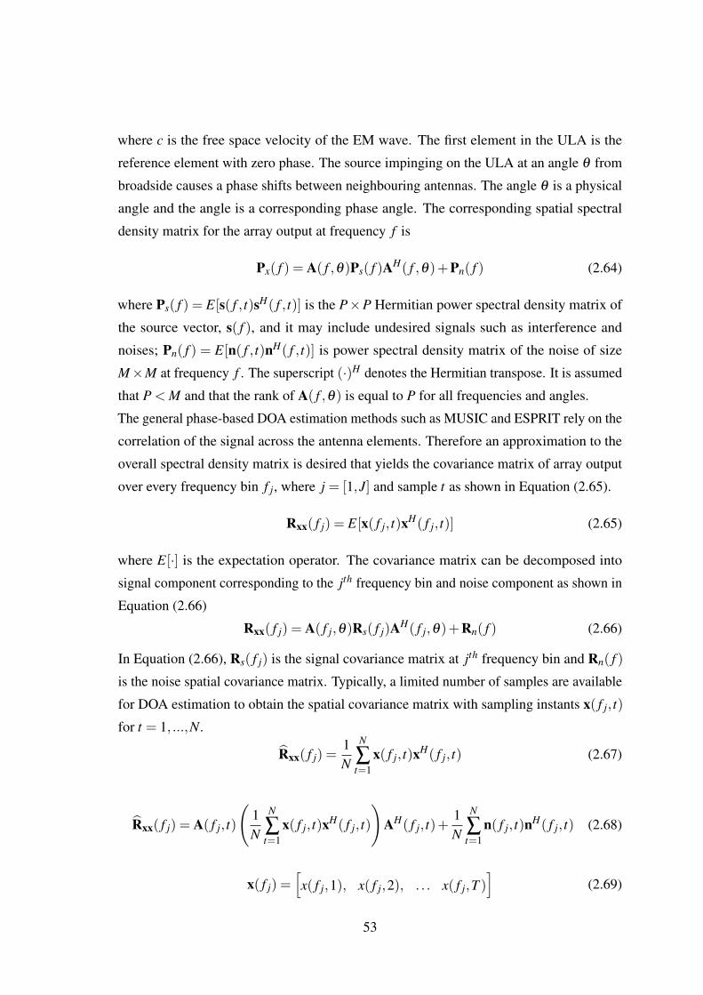
where c is the free space velocity of the EM wave. The first element in the ULA is the
reference element with zero phase. The source impinging on the ULA at an angle θ from
broadside causes a phase shifts between neighbouring antennas. The angle θ is a physical
angle and the angle is a corresponding phase angle. The corresponding spatial spectral
density matrix for the array output at frequency f is
Px( f ) = A( f ,θ)Ps( f )AH( f ,θ)+Pn( f ) (2.64)
where Ps( f ) = E[s( f , t)sH( f , t)] is the P×P Hermitian power spectral density matrix of
the source vector, s( f ), and it may include undesired signals such as interference and
noises; Pn( f ) = E[n( f , t)nH( f , t)] is power spectral density matrix of the noise of size
M×M at frequency f . The superscript (·)H denotes the Hermitian transpose. It is assumed
that P < M and that the rank of A( f ,θ) is equal to P for all frequencies and angles.
The general phase-based DOA estimation methods such as MUSIC and ESPRIT rely on the
correlation of the signal across the antenna elements. Therefore an approximation to the
overall spectral density matrix is desired that yields the covariance matrix of array output
over every frequency bin f j, where j = [1,J] and sample t as shown in Equation (2.65).
Rxx( f j) = E[x( f j, t)xH( f j, t)] (2.65)
where E[·] is the expectation operator. The covariance matrix can be decomposed into
signal component corresponding to the jth frequency bin and noise component as shown in
Equation (2.66)
Rxx( f j) = A( f j,θ)Rs( f j)AH( f j,θ)+Rn( f ) (2.66)
In Equation (2.66), Rs( f j) is the signal covariance matrix at jth frequency bin and Rn( f )
is the noise spatial covariance matrix. Typically, a limited number of samples are available
for DOA estimation to obtain the spatial covariance matrix with sampling instants x( f j, t)
for t = 1, ...,N.
Rxx( f j) =1N
N
∑t=1
x( f j, t)xH( f j, t) (2.67)
Rxx( f j) = A( f j, t)
(1N
N
∑t=1
x( f j, t)xH( f j, t)
)AH( f j, t)+
1N
N
∑t=1
n( f j, t)nH( f j, t) (2.68)
x( f j) =[x( f j,1), x( f j,2), . . . x( f j,T )
](2.69)
53

Here t is the sample index and x( f j) is the data matrix at frequency f j. An adequate
observation period, containing N number of samples must be chosen to facilitate the
sample covariance matrices Ps =1N ∑
Nt=1 s( f j, t)sH( f j, t) and Pn =
1N ∑
Nt=1 n( f j, t)nH( f j, t)
to model signal Ps and noise Pn covariance matrices respectively.
2.8.3 DOA Estimation of Wideband Sources
The DOA estimation of wideband sources, based on each of the discrete frequency bins are
classified as incoherent methods and coherent methods. The wideband DOA estimation by
utilizing narrowband DOA estimation methods at each frequency bin and then combined
to obtain the wide-band estimation is presented in this section. This approach is called
incoherent approach. The subspace-based MUSIC algorithm decomposes the sample
covariance matrix into subspace spanned by signal and noise components. A generic
representation of the covariance matrix is of the form
Rxx( f j) = A( f j,θ)Rs( f j)AH( f j,θ)+Rn( f ) (2.70)
The covariance matrix of Equation (2.70) can be decomposed using EVD as shown in
Equation (2.71)
Rxx( f j) =[Us( f j) Un( f j)
][∑s( f j) 0
0 ∑n( f j)
][UH
s ( f j)
UHn ( f j)
](2.71)
where the ∑s( f j) and ∑n( f j) are the eigen values of the covariance matrices corresponding
the signal subspace and noise subspace respectively for the jth frequency bin. These eigen
values are sorted in the descending order of the diagonal matrix as shown in Equations
(2.72 and 2.73). The matrices Us( f j) and Un( f j) in Equation (2.71) are signal and noise
subspaces, respectively for the jth frequency bin.
∑s( f j) = diag
[σ1( f j) . . . σP( f j)
](2.72)
∑n( f j) = diag
[σP+1( f j) . . . σM( f j)
](2.73)
The P number of eigen values denoting σ1( f j) > σ2( f j) > · · · > σP( f j) are principal
components P signal sources and the remaining σP+1( f j) = σP+2( f j) = · · · = σM( f j)
correspond to the additive noise of the signal;
The standard assumptions of spatially uncorrelated and identically distributed noise ensure
54
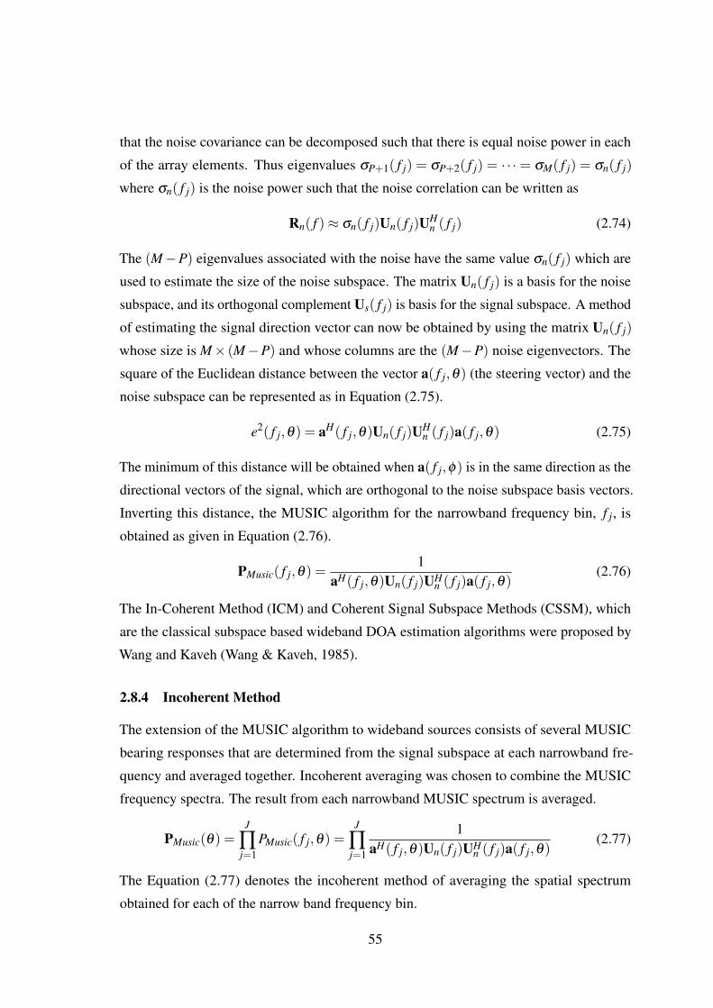
that the noise covariance can be decomposed such that there is equal noise power in each
of the array elements. Thus eigenvalues σP+1( f j) = σP+2( f j) = · · · = σM( f j) = σn( f j)
where σn( f j) is the noise power such that the noise correlation can be written as
Rn( f )≈ σn( f j)Un( f j)UHn ( f j) (2.74)
The (M−P) eigenvalues associated with the noise have the same value σn( f j) which are
used to estimate the size of the noise subspace. The matrix Un( f j) is a basis for the noise
subspace, and its orthogonal complement Us( f j) is basis for the signal subspace. A method
of estimating the signal direction vector can now be obtained by using the matrix Un( f j)
whose size is M× (M−P) and whose columns are the (M−P) noise eigenvectors. The
square of the Euclidean distance between the vector a( f j,θ) (the steering vector) and the
noise subspace can be represented as in Equation (2.75).
e2( f j,θ) = aH( f j,θ)Un( f j)UHn ( f j)a( f j,θ) (2.75)
The minimum of this distance will be obtained when a( f j,φ) is in the same direction as the
directional vectors of the signal, which are orthogonal to the noise subspace basis vectors.
Inverting this distance, the MUSIC algorithm for the narrowband frequency bin, f j, is
obtained as given in Equation (2.76).
PMusic( f j,θ) =1
aH( f j,θ)Un( f j)UHn ( f j)a( f j,θ)
(2.76)
The In-Coherent Method (ICM) and Coherent Signal Subspace Methods (CSSM), which
are the classical subspace based wideband DOA estimation algorithms were proposed by
Wang and Kaveh (Wang & Kaveh, 1985).
2.8.4 Incoherent Method
The extension of the MUSIC algorithm to wideband sources consists of several MUSIC
bearing responses that are determined from the signal subspace at each narrowband fre-
quency and averaged together. Incoherent averaging was chosen to combine the MUSIC
frequency spectra. The result from each narrowband MUSIC spectrum is averaged.
PMusic(θ) =J
∏j=1
PMusic( f j,θ) =J
∏j=1
1aH( f j,θ)Un( f j)UH
n ( f j)a( f j,θ)(2.77)
The Equation (2.77) denotes the incoherent method of averaging the spatial spectrum
obtained for each of the narrow band frequency bin.
55

2.8.5 Coherent Signal Subspace Method
The Coherent Signal-Subspace Method (CSSM) is one of the widely adopted techniques
and it is based on focusing matrices. Wang and Kaveh (Wang & Kaveh, 1985) proposed
the CSSM approach in which a transformation matrix, transforms the covariance matrix
and negates the influence of the frequencies other than the center frequency. After transfor-
mation, the covariance matrix represents a narrowband signal for center frequency.
The jth frequency bin of the observed data sample x( f j, t) and its covariance matrix shall be
computed as shown in Equation (2.67). In CSSM method, data sample corresponding to jth
frequency bin is transformed to a center frequency f0. This transformation is accomplished
by focussing the signal subspace components of the data matrix to the center frequency
(Doron & Weiss, 1992). The focussing of discrete frequencies is achieved by Equation
(2.78).
y( f j, t) = T( f j)x( f j, t) (2.78)
The focussing matrix T( f j) defined in (Yoon, Kaplan, & McClellan, 2006) is represented
in Equation (2.79).
T( f j) =[ei(k j−k0)sinθ , ei(k j−k0)d sinθ , . . . ei(k j−k0)(M−1)d sinθ )
](2.79)
Here the k j is the wave number corresponding to jth frequency bin and k0 is wave number
corresponding to focussing frequency. Typically, the mid frequency of the wideband signal
is chosen as the center frequency. The sample covariance matrix of jth frequency bin after
focussing is obtained by
Ryy( f j) = E[y( f j, t)yH( f j, t)] (2.80)
The CSSM method of wideband DOA estimation using the classical MUSIC algorithm is
computed through the Equation (2.81).
PMusic(θ) =J
∏j=1
1aH( f0,θ)Un( f j)UH
n ( f j)a( f0,θ)(2.81)
In Equation (2.81), Un( f j) is the noise subspace corresponding to covariance matrix of
jth frequency bin Ryy( f j). The product of noise subspaces of all the frequency bins of
the covariance matrix is computed. The array steering vector a( f0,θ) corresponding to
the focussing frequency acts as actual signal subspace which is computed as defined in
Equation (2.63).
56

Several researchers (Doran, Doron, Weiss, et al., 1993; Di Claudio & Parisi, 2001; Yoon
et al., 2006; Zhang, Dai, & Ye, 2010; Yu, Liu, Huang, Zhou, & Xu, 2007; Sellone, 2006)
have attempted to improve the focussing matrix by several techniques. Also the focusing
matrix is parametrized to compute its focussing loss, and thus to relate the inaccuracies of
the estimations is also addressed in the literature.
The CSSM attempts to focus (transform) its signal subspace components to a determined
discrete frequency and averages to produce the search vector for the MUSIC like algorithm.
A method named Array Manifold Interpolation (AMI) (Doran et al., 1993) attempts to lin-
early interpolate the array manifold vector for a desired frequency. These methods provide
a array manifold interpolation matrix, which separates array manifold vector from the array
geometry and direction θ . Further to CSSM, a Weighted Average of Signal Subspaces
(WAVES) method (Di Claudio & Parisi, 2001) was developed by authors Di and Parisi.
In WAVES, the signal subspace components subjected to weighed averaging to improve
the focussing of the signal subspace. The Test of Orthogonality of Projected Subspaces
(TOPS) proposed in (Yoon et al., 2006) for wideband DOA estimation accomplishes an
intermediate performance between incoherent and coherent methods. Subsequently, an
Extended TOPS (ETOPS) (Zhang et al., 2010) algorithm is based on incoherent method
and TOPS algorithm further improved the focussing of signal subspaces at an reference
frequency. The orthogonality between the signal and noise subspaces for each of the
frequency components of the incoming sources is evaluated through TOFS method (Yu
et al., 2007), to improve the focussing of signal subspaces over the CSSM method. The
Robust Coherent Signal Subspace (R-CSM) (Sellone, 2006) proposed by Fabrizio Sellone
shows a novel design of focussing matrices by minimizing the subspace focussing errors by
optimising the Rotational Signal Subspace and Signal subspace transformation of focussing
matrices. The Wideband-Sparse Spectrum Fitting (W-SpSF) estimation proposed by He
et.al. in (He, Shi, Huang, & So, 2015) leverages the increased degrees of freedom of sparse
spatial sampling available through co-array for under determined DOA.
2.9 Summary
This chapter aimed to present an overview of multi-disciplinary attributes of the broad
domain of DOA estimation. It has provided a review of the basic concepts of antenna,
antenna array and DOA estimation algorithms along with the associated mathematical
techniques. After a brief discussion on important performance parameters of antenna, a
57

succinct review of various configurations such as 1D, 2D and 3D antenna arrays is presented
in this chapter. The progression in the DOA estimation algorithms from Fourier based to
subspace techniques has also been covered in this chapter with pertinent technical details.
The assumptions associated with the determination of radiation pattern of antenna arrays
used in DOA estimation algorithms have been briefly explained. The analytical details of
classical subspace techniques like MUSIC and ESPRIT which are either extensively used
or referred in this thesis have been dealt in detail. This chapter has presented a discussion
on the existing techniques for the estimation of DOA of non-stationary sources. A review
of available techniques for the estimation of DOA of wideband sources is also included
in this chapter. The implicit/explicit constraints as well as the limitations of conventional
antenna arrays and the existing DOA estimation algorithms are highlighted with a view to
facilitate better appreciation of the novelties and the significance of the analysis/results to
be presented in the subsequent chapters of this thesis.
58
Chapter 3
Formulation and Analysis of a Closed Form Solution for Two
Dimensional DOA Estimation
3.1 Introduction
This chapter presents a formulation, for the minimization of computational complexity of
two-dimensional DOA estimation algorithm for single incoming source scenario. Towards
this end, a closed form expression for two-dimensional DOA estimation using the MUSIC
algorithm is proposed which involves only one-dimensional search. This task has been
accomplished by a novel one-dimensional antenna array configuration with its alternate
array element’s orthogonal orientation. These elements receive both the horizontal and
vertical polarized field components simultaneously and these components are processed for
2D-DOA estimation. With prior knowledge of the analytical expressions for the radiation
patterns of typical array elements, a closed form expression has been derived relating
the azimuthal angle φ and elevation angle θ of DOA through the ratio of the amplitudes
of horizontally and vertically polarized received fields. This concept is illustrated using
the open ended Rectangular Wave Guide (RWG) and Circular Wave Guide (CWG) as an
antenna element.
3.2 Review of 2D-DOA Estimation Techniques
A basic review on antenna array configuration and DOA estimation algorithms has already
been presented in Chapter 2. In the discussion of antenna array for 2D-DOA estimation
covered in Chapter 2, the emphasis was on antenna elements having identical (single)
polarization only. In this section, the significance of diversely polarized antenna elements
in DOA estimation is reviewed. Generally, two-dimensional array configurations such as
planar, circular or three-dimensional array with linear subarrays along the three axes are
used for the 2D-DOA estimation (N. Tayem & Kwon, 2005; Manikas, Alexiou, & Karimi,
1997). The general performance of a DOA estimation system is also directly influenced by
59
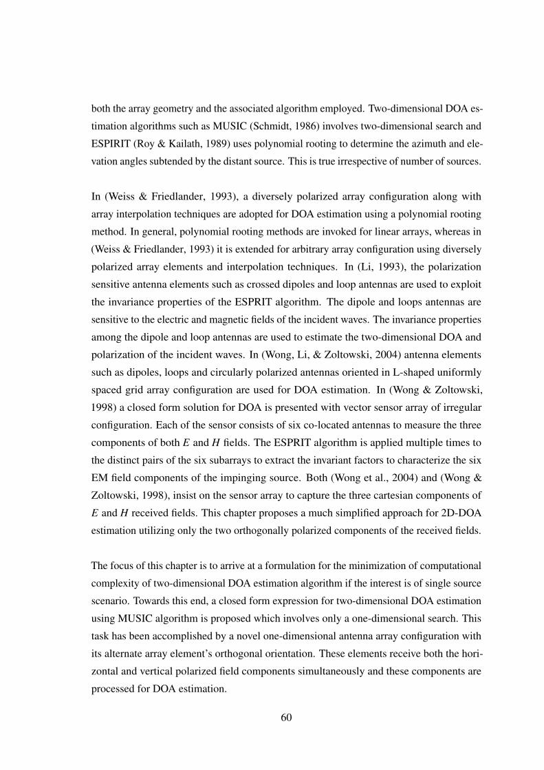
both the array geometry and the associated algorithm employed. Two-dimensional DOA es-
timation algorithms such as MUSIC (Schmidt, 1986) involves two-dimensional search and
ESPIRIT (Roy & Kailath, 1989) uses polynomial rooting to determine the azimuth and ele-
vation angles subtended by the distant source. This is true irrespective of number of sources.
In (Weiss & Friedlander, 1993), a diversely polarized array configuration along with
array interpolation techniques are adopted for DOA estimation using a polynomial rooting
method. In general, polynomial rooting methods are invoked for linear arrays, whereas in
(Weiss & Friedlander, 1993) it is extended for arbitrary array configuration using diversely
polarized array elements and interpolation techniques. In (Li, 1993), the polarization
sensitive antenna elements such as crossed dipoles and loop antennas are used to exploit
the invariance properties of the ESPRIT algorithm. The dipole and loops antennas are
sensitive to the electric and magnetic fields of the incident waves. The invariance properties
among the dipole and loop antennas are used to estimate the two-dimensional DOA and
polarization of the incident waves. In (Wong, Li, & Zoltowski, 2004) antenna elements
such as dipoles, loops and circularly polarized antennas oriented in L-shaped uniformly
spaced grid array configuration are used for DOA estimation. In (Wong & Zoltowski,
1998) a closed form solution for DOA is presented with vector sensor array of irregular
configuration. Each of the sensor consists of six co-located antennas to measure the three
components of both E and H fields. The ESPRIT algorithm is applied multiple times to
the distinct pairs of the six subarrays to extract the invariant factors to characterize the six
EM field components of the impinging source. Both (Wong et al., 2004) and (Wong &
Zoltowski, 1998), insist on the sensor array to capture the three cartesian components of
E and H received fields. This chapter proposes a much simplified approach for 2D-DOA
estimation utilizing only the two orthogonally polarized components of the received fields.
The focus of this chapter is to arrive at a formulation for the minimization of computational
complexity of two-dimensional DOA estimation algorithm if the interest is of single source
scenario. Towards this end, a closed form expression for two-dimensional DOA estimation
using MUSIC algorithm is proposed which involves only a one-dimensional search. This
task has been accomplished by a novel one-dimensional antenna array configuration with
its alternate array element’s orthogonal orientation. These elements receive both the hori-
zontal and vertical polarized field components simultaneously and these components are
processed for DOA estimation.
60
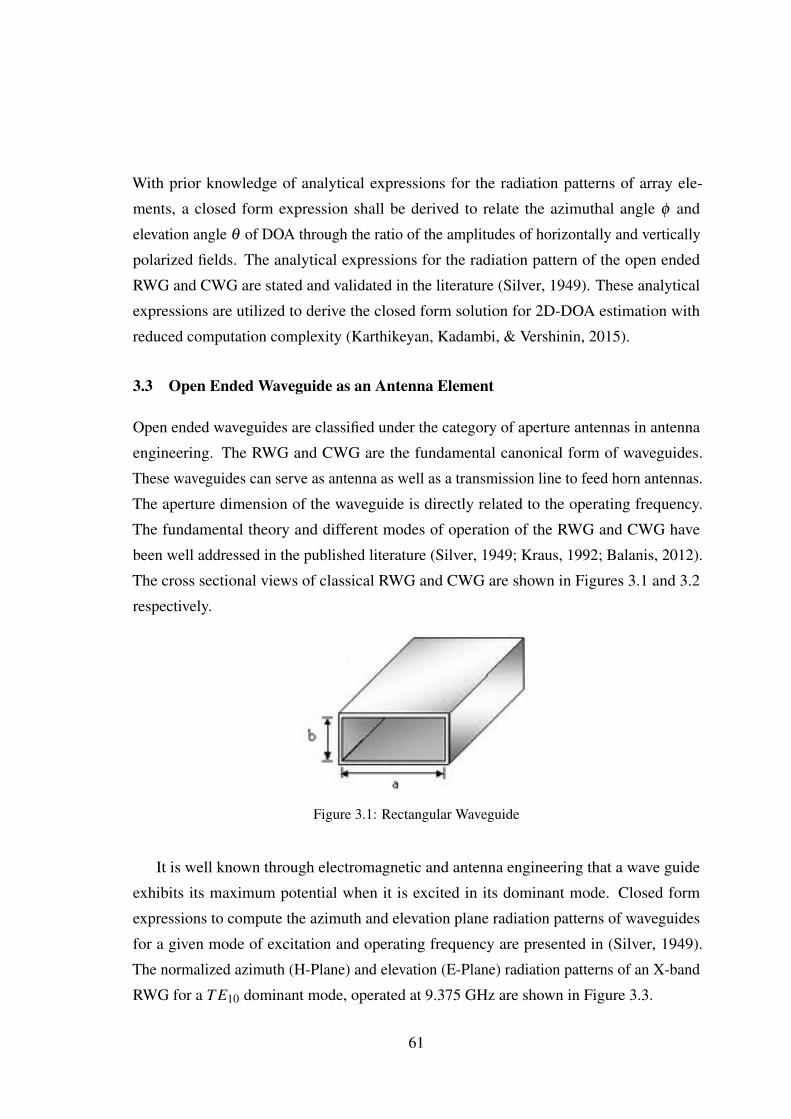
With prior knowledge of analytical expressions for the radiation patterns of array ele-
ments, a closed form expression shall be derived to relate the azimuthal angle φ and
elevation angle θ of DOA through the ratio of the amplitudes of horizontally and vertically
polarized fields. The analytical expressions for the radiation pattern of the open ended
RWG and CWG are stated and validated in the literature (Silver, 1949). These analytical
expressions are utilized to derive the closed form solution for 2D-DOA estimation with
reduced computation complexity (Karthikeyan, Kadambi, & Vershinin, 2015).
3.3 Open Ended Waveguide as an Antenna Element
Open ended waveguides are classified under the category of aperture antennas in antenna
engineering. The RWG and CWG are the fundamental canonical form of waveguides.
These waveguides can serve as antenna as well as a transmission line to feed horn antennas.
The aperture dimension of the waveguide is directly related to the operating frequency.
The fundamental theory and different modes of operation of the RWG and CWG have
been well addressed in the published literature (Silver, 1949; Kraus, 1992; Balanis, 2012).
The cross sectional views of classical RWG and CWG are shown in Figures 3.1 and 3.2
respectively.
Figure 3.1: Rectangular Waveguide
It is well known through electromagnetic and antenna engineering that a wave guide
exhibits its maximum potential when it is excited in its dominant mode. Closed form
expressions to compute the azimuth and elevation plane radiation patterns of waveguides
for a given mode of excitation and operating frequency are presented in (Silver, 1949).
The normalized azimuth (H-Plane) and elevation (E-Plane) radiation patterns of an X-band
RWG for a T E10 dominant mode, operated at 9.375 GHz are shown in Figure 3.3.
61

Figure 3.2: Circular Waveguide
Figure 3.3: Normalized Radiation Pattern of a RWG
The Figure 3.4 indicate the copolar and cross polar components of the radiation of
RWG. The significant difference between the copolar and cross polar justifies that, the
cross polar component shall be ignored in the computations.
3.3.1 Proposed Orthogonally Polarized Linear Array Configuration
The RWG array is chosen for the proposed research based on the strong theoretical and
practical considerations of RWG as an antenna element. The Orthogonally Polarized Linear
Array (OPLA) configuration is proposed as shown in the Figure 3.5. In the proposed array
configuration shown in Figure 3.6, the RWG elements are arranged in a straight line with
the adjacent elements rotated by 90◦. The adjacent elements of the array are orthogonally
62
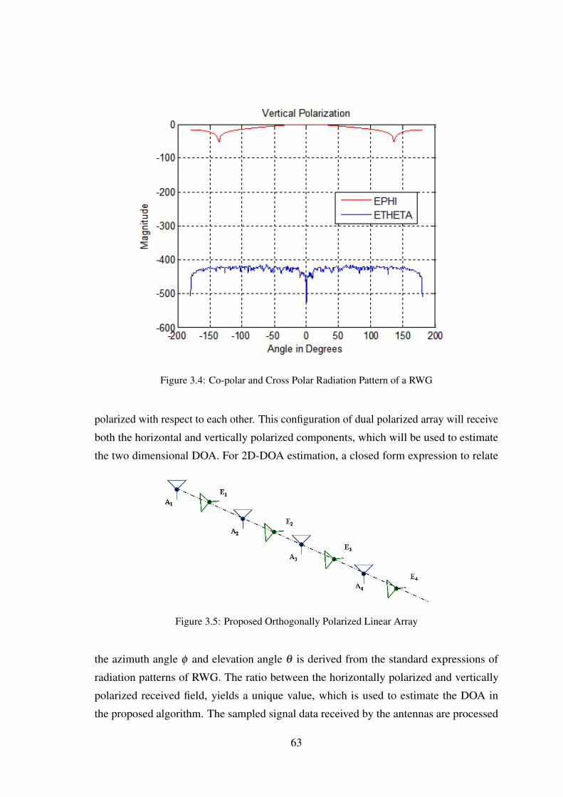
Figure 3.4: Co-polar and Cross Polar Radiation Pattern of a RWG
polarized with respect to each other. This configuration of dual polarized array will receive
both the horizontal and vertically polarized components, which will be used to estimate
the two dimensional DOA. For 2D-DOA estimation, a closed form expression to relate
Figure 3.5: Proposed Orthogonally Polarized Linear Array
the azimuth angle φ and elevation angle θ is derived from the standard expressions of
radiation patterns of RWG. The ratio between the horizontally polarized and vertically
polarized received field, yields a unique value, which is used to estimate the DOA in
the proposed algorithm. The sampled signal data received by the antennas are processed
63
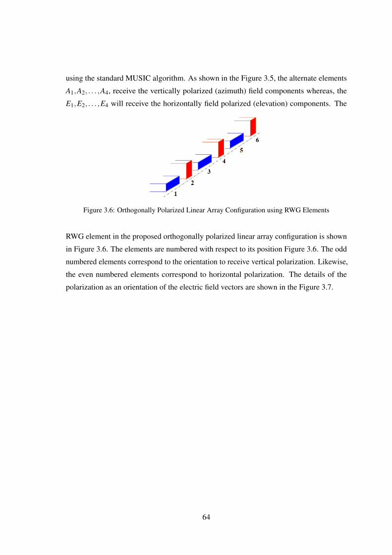
using the standard MUSIC algorithm. As shown in the Figure 3.5, the alternate elements
A1,A2, . . . ,A4, receive the vertically polarized (azimuth) field components whereas, the
E1,E2, . . . ,E4 will receive the horizontally field polarized (elevation) components. The
Figure 3.6: Orthogonally Polarized Linear Array Configuration using RWG Elements
RWG element in the proposed orthogonally polarized linear array configuration is shown
in Figure 3.6. The elements are numbered with respect to its position Figure 3.6. The odd
numbered elements correspond to the orientation to receive vertical polarization. Likewise,
the even numbered elements correspond to horizontal polarization. The details of the
polarization as an orientation of the electric field vectors are shown in the Figure 3.7.
64
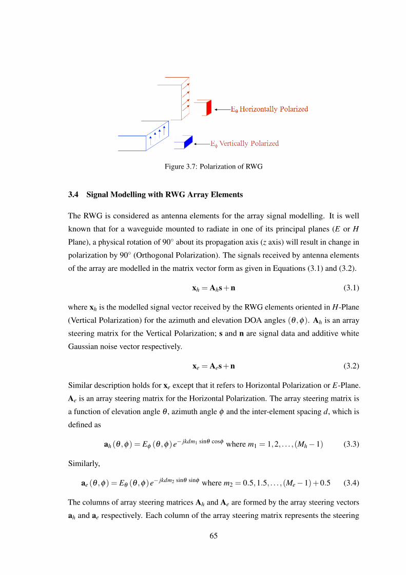
Figure 3.7: Polarization of RWG
3.4 Signal Modelling with RWG Array Elements
The RWG is considered as antenna elements for the array signal modelling. It is well
known that for a waveguide mounted to radiate in one of its principal planes (E or H
Plane), a physical rotation of 90◦ about its propagation axis (z axis) will result in change in
polarization by 90◦ (Orthogonal Polarization). The signals received by antenna elements
of the array are modelled in the matrix vector form as given in Equations (3.1) and (3.2).
xh = Ahs+n (3.1)
where xh is the modelled signal vector received by the RWG elements oriented in H-Plane
(Vertical Polarization) for the azimuth and elevation DOA angles (θ ,φ). Ah is an array
steering matrix for the Vertical Polarization; s and n are signal data and additive white
Gaussian noise vector respectively.
xe = Aes+n (3.2)
Similar description holds for xe except that it refers to Horizontal Polarization or E-Plane.
Ae is an array steering matrix for the Horizontal Polarization. The array steering matrix is
a function of elevation angle θ , azimuth angle φ and the inter-element spacing d, which is
defined as
ah (θ ,φ) = Eφ (θ ,φ)e− jkdm1 sinθ cosφ where m1 = 1,2, . . . ,(Mh−1) (3.3)
Similarly,
ae (θ ,φ) = Eθ (θ ,φ)e− jkdm2 sinθ sinφ where m2 = 0.5,1.5, . . . ,(Me−1)+0.5 (3.4)
The columns of array steering matrices Ah and Ae are formed by the array steering vectors
ah and ae respectively. Each column of the array steering matrix represents the steering
65

vector of the corresponding source angle (θ ,φ). For the case of a single source, the array
steering matrix has only one column, corresponding to the steering vector of the impinging
source angle (θ ,φ).
In Equations (3.3) and (3.4), Mh and Me represent the number of antenna elements oriented
in H-plane and E-plane respectively. k represents free space wave number. Typically, the
inter-element spacing d is such that λ
4 ≤ d ≤ λ
2 , λ being the wavelength. The Eφ (θ ,φ)
and Eθ (θ ,φ) are the amplitudes of vertically and horizontally polarized field components
of the radiation pattern at (θ ,φ).
The computation of the sample covariance matrix to invoke MUSIC algorithm (Schmidt,
1986) is carried out using Equation (3.5).
Rxx = E[xexH
e]
(3.5)
In Equation (3.5), E[.] is the expectation operator and (.)H denotes the Hermitian conjugate.
The covariance matrix Rxx can also be constructed using xh data. The covariance matrix
can be decomposed into signal and noise components through eigen decomposition shown
in Equation (3.6).
Rxx = ASAH +σ2I (3.6)
where S = E[ssH ] is the signal covariance matrix; A denotes the matrix representation
of the array steering vector for the respective polarization as shown in Equations (3.3)
and (3.4). σ2 is the noise covariance, I is the identity matrix. The eigen vectors of the
covariance matrix are decomposed into signal and noise subspace as stated in Equation
(3.6) which are orthogonal to each other. The peak magnitude of MUSIC algorithm for the
two-dimensional DOA estimation is given in Equation (3.7).
argmax(θ ,φ)
P(θ ,φ) =1
a(θ ,φ)VnVHn aH (θ ,φ)
(3.7)
where a(θ ,φ) is a search vector. The matrix Vn spans the noise subspace vectors in its
columns, which are the eigenvectors whose eigenvalues are equal to the σ2.
3.5 2D-DOA Estimation Using Closed Form Solutions
For two-dimensional DOA estimation in the case of a single source, the two-dimensional
search Equation (3.7) can be reduced to one-dimensional search which constitutes the
66
proposed research contribution of this chapter. The two-dimensional search vector a(θ ,φ)is reduced to one-dimension by deriving compact expressions which relates the angle θ in
terms of angle φ through the ratio of amplitudes of vertical polarized (Eφ ) and horizontal
polarized (Eθ ) field components received by the RWG elements of the array.
3.5.1 Derivation to Relate Azimuth and Elevation DOA Angles with RWG
The analytical expressions of Eθ (Horizontal Polarization) and Eφ (Vertical Polarization)
components of radiation patterns of the RWG with a dominant T E10 mode of propagation
are given by Equations (3.8) and (3.9), respectively along with equation (3.10) (Silver,
1949). These closed form expressions are used to compute the E-Plane (horizontal) and
H-Plane (vertical) polarized radiation pattern for a given operating frequency (9.375 GHz).
Eθ (θ ,φ) =−(
µ
ε
)1/2 πa2b2λ 2R
cosφ
[β10
k+ cosθ
]Ψ(θ ,φ) (3.8)
Eφ (θ ,φ) =−(
µ
ε
)1/2 πa2b2λ 2R
sinφ
[1+
β10
kcosθ
]Ψ(θ ,φ) (3.9)
where,
Ψ(θ ,φ) =
[cos(
πaλ
sinθ cosφ)(
πaλ
sinθ cosφ)2−
(π
a
)2
][sin(
πbλ
sinθ sinφ)(
πbλ
sinθ sinφ) ]
(3.10)
For a rectangular waveguide, β10 is computed by
βmn =√
k2− k2mn (3.11)
where
kmn =
√(mπ
a
)2+(nπ
b
)2(3.12)
where θ is the elevation angle,
φ is the azimuth angle,
µ is the free space permeability,
ε is the free space permittivity
λ is the wavelength,
k is the wave number,
a is the width of the waveguide aperture,
b is the height of the waveguide aperture,
β10 is the propagation constant for the waveguide excited in dominant mode (m = 1,n = 0),
67

R is the distance between a reference point and a far-field distant point.
The ratio between the horizontal and vertical polarized field components of the received
signal shall be derived as follows. Let
X =|Eθ (θ ,φ)|∣∣Eφ (θ ,φ)
∣∣ (3.13)
X denotes the ratio of amplitudes of horizontal and vertical polarized field components
received by the RWG elements. With the substitution of Equations (3.8) and (3.9) in
Equation (3.13).
X =sinφ
[1+ β10
k cosθ
]cosφ
[cosθ + β10
k
] (3.14)
Further simplification of Equation (3.14) yields the separable closed form expressions
relating the azimuth φ and elevation θ angles as shown in Equation (3.15) and (3.16).
φ = tan−1
X(
cosθ + β10k
)1+ β10
k cosθ
(3.15)
θ = cos−1
(tanφ −X β10
k
X− β10k tanφ
)(3.16)
The exponential term of Equation (3.3) can be rewritten as shown in Equation (3.17) with
the substitution of Equation (3.15).
e− j 2π
λd sinθ cos
tan−1
X(
cosθ+β10
k
)1+
β10k cosθ
(3.17)
Thus, the exponential term of Equation(3.17) only involves the elevation angle θ . Similarly,
the exponential term of Equation (3.3) shall also be rewritten after substituting Equation
(3.16) in it. As a result, the exponential term of Equation (3.3) can be written to involve
only the azimuth angle φ .
e− j 2π
λd sin
(cos−1
(tanφ−X
β10k
X− β10k tanφ
))cosφ
(3.18)
The expressions (3.17) and (3.18) which relate the 2D-DOA (θ ,φ) with only one angle say
elevation θ (or azimuth φ ) shall be utilized in the two-dimensional search vector ah (θ ,φ)
in Equation (3.7) of the MUSIC algorithm.
68

3.5.2 Derivation to Relate Azimuth and Elevation DOA Angles with CWG
The derivation described for RWG has been extended to the case wherein the RWG is
replaced by a CWG. Similar to the RWG, the analytical expressions of Eθ (θ ,φ) and
Eφ (θ ,φ) components of radiation patterns of CWG with the T E11 dominant mode are
given by Equations (3.19) and (3.20) (Silver, 1949).
Eθ (θ ,φ) =kρωµ
2R
[1+
β11
kcosθ
]J1 (k11ρ)
J1 (kρ sinθ)
kρ sinθsinφ (3.19)
Eφ (θ ,φ) =kρωµ
2R
[cosθ +
β11
k
]J1 (k11ρ)
J′1 (kρ sinθ)
1−(
kρ sinθ
k11
)2 cosφ (3.20)
For the dominant T E11 mode of a circular waveguide, β11 is computed as
β11 =
√k2−
(1.841
ρ
)2
where ρ is the radius of the circular waveguide, k is the wave number, J1(.) is the first
order Bessel function and J′1(.) is the derivative of the first order Bessel function. Similar
to Equation (3.13), the ratio of amplitude of Eθ and Eφ field components received by the
CWG elements of the array can be related through Equation (3.21).
X =|Eθ (θ ,φ)|∣∣Eφ (θ ,φ)
∣∣ = 1+ β11k cosθ
cosθ + β11k
J1(kρ sinθ)kρ sinθ
J′1(kρ sinθ)
1−(
kρ sinθ
k11
)2
tanφ (3.21)
For the CWG, only the azimuth angle φ can be related in-terms of the elevation angle θ as
shown in Equation (3.22).
φ = tan−1
X(
cosθ + β11k
)1+ β11
k cosθ
J′m (kρ sinθ)
1−(
k sinθ
k11
)2kρ sinθ
J1 (kρ sinθ)
(3.22)
The exponential term of Equations (3.3) can be represented as shown in Equation (3.23)
after the substitution of Equation (3.22).
e
− jkd sinθ cos
tan−1
X(
cosθ+β11
k
)1+
β11k cosθ
J′m(kρ sinθ)
1−(
k sinθk11
)2kρ sinθ
J1(kρ sinθ)
(3.23)
The derived Equation (3.22), relates the azimuth angle φ in-terms of only the elevation
angle θ as shown in expression (3.23).
69
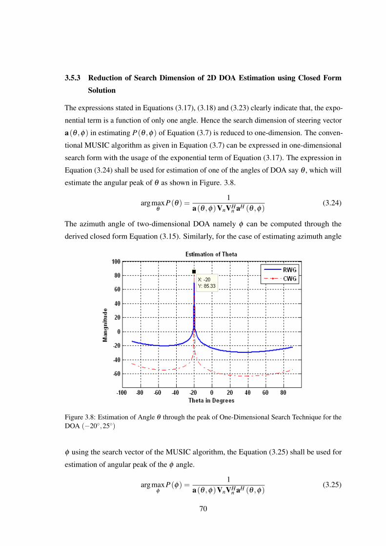
3.5.3 Reduction of Search Dimension of 2D DOA Estimation using Closed FormSolution
The expressions stated in Equations (3.17), (3.18) and (3.23) clearly indicate that, the expo-
nential term is a function of only one angle. Hence the search dimension of steering vector
a(θ ,φ) in estimating P(θ ,φ) of Equation (3.7) is reduced to one-dimension. The conven-
tional MUSIC algorithm as given in Equation (3.7) can be expressed in one-dimensional
search form with the usage of the exponential term of Equation (3.17). The expression in
Equation (3.24) shall be used for estimation of one of the angles of DOA say θ , which will
estimate the angular peak of θ as shown in Figure. 3.8.
argmaxθ
P(θ) =1
a(θ ,φ)VnVHn aH (θ ,φ)
(3.24)
The azimuth angle of two-dimensional DOA namely φ can be computed through the
derived closed form Equation (3.15). Similarly, for the case of estimating azimuth angle
Figure 3.8: Estimation of Angle θ through the peak of One-Dimensional Search Technique for theDOA (−20◦,25◦)
φ using the search vector of the MUSIC algorithm, the Equation (3.25) shall be used for
estimation of angular peak of the φ angle.
argmaxφ
P(φ) =1
a(θ ,φ)VnVHn aH (θ ,φ)
(3.25)
70
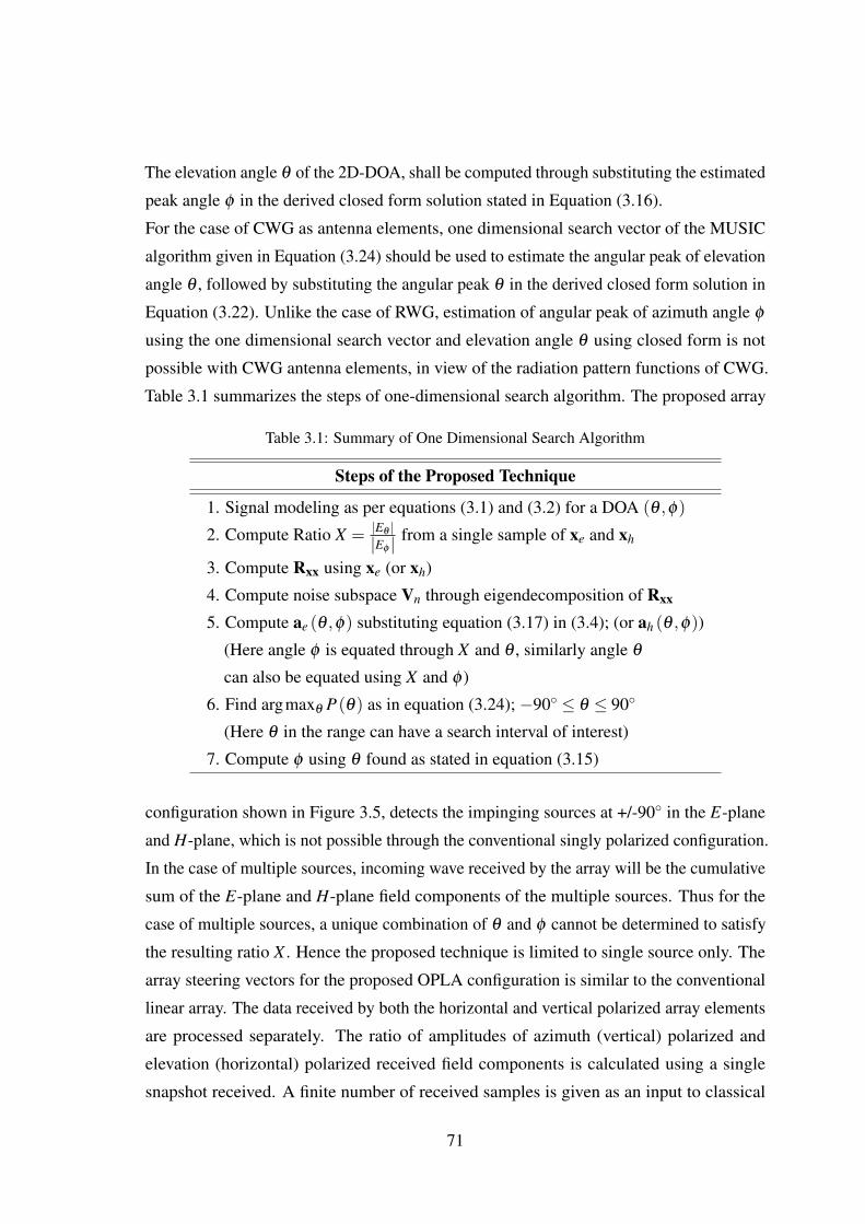
The elevation angle θ of the 2D-DOA, shall be computed through substituting the estimated
peak angle φ in the derived closed form solution stated in Equation (3.16).
For the case of CWG as antenna elements, one dimensional search vector of the MUSIC
algorithm given in Equation (3.24) should be used to estimate the angular peak of elevation
angle θ , followed by substituting the angular peak θ in the derived closed form solution in
Equation (3.22). Unlike the case of RWG, estimation of angular peak of azimuth angle φ
using the one dimensional search vector and elevation angle θ using closed form is not
possible with CWG antenna elements, in view of the radiation pattern functions of CWG.
Table 3.1 summarizes the steps of one-dimensional search algorithm. The proposed array
Table 3.1: Summary of One Dimensional Search Algorithm
Steps of the Proposed Technique
1. Signal modeling as per equations (3.1) and (3.2) for a DOA (θ ,φ)
2. Compute Ratio X = |Eθ ||Eφ | from a single sample of xe and xh
3. Compute Rxx using xe (or xh)
4. Compute noise subspace Vn through eigendecomposition of Rxx
5. Compute ae (θ ,φ) substituting equation (3.17) in (3.4); (or ah (θ ,φ))
(Here angle φ is equated through X and θ , similarly angle θ
can also be equated using X and φ )
6. Find argmaxθ P(θ) as in equation (3.24); −90◦ ≤ θ ≤ 90◦
(Here θ in the range can have a search interval of interest)
7. Compute φ using θ found as stated in equation (3.15)
configuration shown in Figure 3.5, detects the impinging sources at +/-90◦ in the E-plane
and H-plane, which is not possible through the conventional singly polarized configuration.
In the case of multiple sources, incoming wave received by the array will be the cumulative
sum of the E-plane and H-plane field components of the multiple sources. Thus for the
case of multiple sources, a unique combination of θ and φ cannot be determined to satisfy
the resulting ratio X . Hence the proposed technique is limited to single source only. The
array steering vectors for the proposed OPLA configuration is similar to the conventional
linear array. The data received by both the horizontal and vertical polarized array elements
are processed separately. The ratio of amplitudes of azimuth (vertical) polarized and
elevation (horizontal) polarized received field components is calculated using a single
snapshot received. A finite number of received samples is given as an input to classical
71

MUSIC algorithm. This is a typical one dimensional DOA estimation. The derived closed
form expressions namely Equations (3.15) and (3.16) for RWG and Equation (3.22) for
CWG are used to compute search in one dimension. With this procedure the azimuth DOA
angle can be estimated using the Equation (3.15) for RWG or Equation (3.22) for CWG.
The estimation of the elevation DOA can be substituted in the closed form expression
to obtain azimuth DOA or vice versa. In this proposed method of 2D-DOA estimation,
search computations are drastically reduced because of closed form relation of azimuth
and elevation angles. In the proposed method, the searching dimension is now reduced to
one dimensional (Equations (3.24) and (3.25)) instead of the two dimensional (Equation
(3.7)) in typical 2D-DOA estimation algorithms.
3.5.4 Simulation Analysis of Proposed One Dimensional Search Technique for 2D-DOA
Conventionally for two-dimensional DOA estimation, a typical planar array configuration
is used. A 2× 2 planar array with RWG elements operating at 9.375 GHz was used to
compute two-dimensional DOA. The signal was modeled for the incoming angles of actual
DOA as stated in Table 3.2. In this analysis, a perfect mounting of the antenna elements in
their principal (E and H) planes without mutual coupling between them is assumed. The
spacing between the elements is λ /4.
The conventional two-dimensional search based MUSIC algorithm (Equation (3.7)) was
used to estimate the φ and θ angles of DOA. Digital data modulated with a sinusoidal
signal of frequency 9.375 GHz is modelled, which forms the spatio-temporal samples, as
an input for the DOA analysis. The AWGN noise is considered with a SNR of 15 dB for
the signal modelled for the array configuration. 100 number of spatio-temporal samples
were considered for the simulation. The estimated DOA angles using the conventional two-
dimensional search of MUSIC algorithm using Equation (3.7) are tabulated in Table 3.2.
The signal was remodelled using Equations (3.1 and 3.2) for the proposed one-dimensional
OPLA configuration for the same φ and θ angles of DOA as used for two-dimensional
search technique of MUSIC. The steps for one-dimensional search algorithm for 2D-DOA
estimation are provided in Table 3.1. The ratio between the horizontal and vertical polarized
component of the impinging signal is computed form the signal model using the Equations
(3.1 and 3.2).
72

Tabl
e3.
2:C
ompa
riso
nof
Ant
enna
Con
figur
atio
nsfo
rDO
Aan
dTi
min
gA
naly
sis
Con
figur
atio
nA
ctua
lE
stim
ated
DO
Aat
Com
puta
tion
Tim
eE
stim
ated
DO
Aat
Com
puta
tion
Tim
eD
OA
1◦Se
arch
Inte
rval
with
1◦Se
arch
Inte
rval
with
0.5◦
Sear
chIn
terv
al0.
5◦Se
arch
Inte
rval
(θ◦ ,
φ◦ )
(θ◦ ,
φ◦ )
(sec
onds
)(θ◦ ,
φ◦ )
(sec
onds
)2x
2Pl
anar
Arr
ay(−
20◦ ,
25◦ )
(−20◦ ,
25◦ )
0.76
2(−
20◦ ,
25◦ )
3.12
0(T
wo-
Dim
ensi
onal
(50◦,−
25◦ )
(50◦,−
25◦ )
0.76
1(5
0◦,−
25◦ )
3.12
0D
OA
Sear
ch)
(−50◦ ,−
25◦ )
(−50◦ ,−
25◦ )
0.76
4(−
50◦ ,−
25◦ )
3.12
0(0◦ ,
0◦)
(0◦ ,
0◦)
0.76
0(0◦ ,
0◦)
3.12
01x
4Pr
opos
edA
rray
(−20◦ ,
25◦ )
(−20◦ ,
25◦ )
0.01
3(−
20◦ ,
25◦ )
0.02
1(O
ne-D
imen
sion
al(5
0◦,−
25◦ )
(50◦,−
25◦ )
0.01
3(5
0◦,−
25◦ )
0.02
2D
OA
Sear
ch)
(−50◦ ,−
25◦ )
(−50◦ ,−
25◦ )
0.01
3(−
50◦ ,−
25◦ )
0.02
5(0◦ ,
0◦)
(0◦ ,
0◦)
0.01
3(0◦ ,
0◦)
0.02
1(1
0◦,9
0◦)
(10◦,9
0◦)
0.01
3(1
0◦,9
0◦)
0.02
1(9
0◦,1
0◦)
(90◦,1
0◦)
0.01
3(9
0◦,1
0◦)
0.02
1
73

The proposed one-dimensional search based MUSIC algorithm as stated in Equation
(3.24) was used to estimate elevation angle θ first and then the azimuth angle φ was
computed through the Equation (3.15). The results of the estimation of 2D-DOA (Table
3.2) through the conventional two-dimensional search approach and the proposed one-
dimensional search technique are found to be exactly the same establishing the validity of
the proposed technique.
The analysis of two-dimensional DOA computations was repeated with the CWG as
array elements which also yielded the same DOA estimation as with RWG. The envelope
of P(θ) of Equation (3.24) simulated with RWG and CWG for the desired elevation
angle, θ = -20◦ is shown in Figure. 3.8. The tabulated computational time in Table 3.2
highlights the reduced computation of the proposed one dimensional search technique
for the estimation of 2D-DOA. Simulations for both the one-dimensional search and
two-dimensional search were performed on Intel core 2 Duo processor of 2.93 GHz
clock speed platform. The computation time for the proposed one dimensional search
technique of 2D-DOA estimation is reduced by a factor of 50 and 150 for 1◦ and 0.5◦ search
intervals respectively, when compared with the conventional two-dimensional MUSIC
search algorithm.
3.5.5 RMSE Analysis
The derived formulation of 2D-DOA estimation with 1D search approach is analysed for
the range of SNR scenario 0 - 30 dB. The simulation for the wide range of SNR scenario is
carried for signal model with DOA angles θ = -20◦, φ = 25◦. The RMSE of the estimation
of elevation angle θ and azimuth angle φ is computed. The average estimation error from
200 simulation iteration for wide range of SNRs are computed and the results are shown in
the Figure 3.9. The results reveal that estimation of θ angle has higher estimation error
when compared to φ estimation error. The geometric configuration of the OPLA is linear.
The spatial covariance of the received data samples is along only one direction, that is the
array axis (x axis). Thus the θ estimation error is more than φ estimation error.
The results of the estimation of 2D-DOA OPLA configuration with one-dimensional
search approach is compared with the conventional 2×2 uniform planar array configuration.
The RMSE of 2D-DOA estimation for 2×2 UPA configuration is shown in Figure 3.10.
The RMSE results shown in Figure 3.10 illustrate the importance of spatial phase variation
with respect to geometric configuration of the array elements. The presence of spatial phase
74
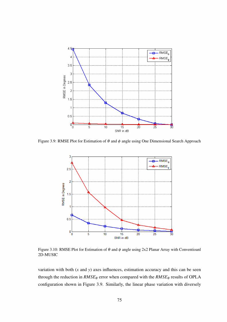
Figure 3.9: RMSE Plot for Estimation of θ and φ angle using One Dimensional Search Approach
Figure 3.10: RMSE Plot for Estimation of θ and φ angle using 2x2 Planar Array with Conventioanl2D-MUSIC
variation with both (x and y) axes influences, estimation accuracy and this can be seen
through the reduction in RMSEθ error when compared with the RMSEθ results of OPLA
configuration shown in Figure 3.9. Similarly, the linear phase variation with diversely
75
polarized array configuration of OPLA is advantageous with the estimation of RMSEφ
with least error, whereas poorer estimation accuracy in RMSEφ is seen with the result of
conventional UPA configuration due to its limited phase variation along x axis.
3.6 Summary
This chapter has presented an elegant one-dimensional search technique for two dimen-
sional DOA estimation involving azimuth and elevation angles of distant sources. The
proposed one-dimensional search is a consequence of utilizing the linear array configura-
tion with alternate elements orthogonally polarized. The distinct feature of the proposed
one-dimensional search technique leading to a significant reduction in the computation time
for two-dimensional DOA estimation using MUSIC algorithm has been illustrated through
the simulation studies. The proposed 2D-DOA estimation using one dimensional search is
applicable only for a single source. Without loss of generality, the proposed formulation
can be extended to any other antenna whose radiation pattern can be represented through
an analytical expression involving separable form of elevation angle θ and azimuth angle
φ .
The OPLA configuration can be used to estimate DOA with classical subspace based tech-
niques. The derived closed form expression relation can be used along with the classical
subspace based techniques to estimate 2D-DOA. The search dimensions are reduced to
minimize the computation intensity in the proposed method. The proposed OPLA configu-
ration minimizes the mutual EM coupling between the adjacent array elements. Reduced
mutual coupling is obtained even when the antenna elements are very close to each other.
76
Chapter 4
Two Dimensional DOA Estimation using Dual Polarized Array for
Single and Multiple Sources
4.1 Introduction
In this chapter, the diversely (dual) polarized array configurations are analysed for their
performance in estimating 2D-DOA of the single and multiple sources. Discussion on
various antenna array configurations for 2D-DOA estimation has been presented in Chapter
2. Subsequently, Chapter 3 covered the significance of antenna arrays with diversely
polarized antenna elements. A novel OPLA configuration has been proposed for 2D-DOA
estimation in Chapter 3. This chapter deals with other types of orthogonal polarized antenna
arrays for 2D-DOA estimation. In this study, from antenna engineering perspective, dual
polarization concept and different antenna array configurations are explored to improve the
accuracy and resolution of DOA. Novel array configurations are proposed, where adjacent
array elements have orthogonal polarization. The simulation studies confirm the proposed
array geometries improve estimation accuracy of 2D-DOA estimations when compared
with the single polarized array configuration.
4.1.1 Antenna Configurations for 2D-DOA Estimation
Typically, one dimensional array is used to estimate 1D-DOA (usually azimuth) and two
or three dimensional array are used for 2D-DOA estimation. The conventional Uniform
Planar Array (UPA) or Uniform Circular Array (UCA) (Balanis, 2012) configurations are
used for the 2D-DOA estimation. Apart from this L-shaped array and 2L shaped array
configurations addressed in (N. A.-H. M. Tayem, 2005; N. Tayem & Kwon, 2005) have
been used for 2D-DOA estimation and involve pair matching computations.
77

4.2 Antenna Element Radiation Pattern in DOA
In the field of the array signal processing (especially in antenna arrays), generally re-
searchers exclude the elemental radiation pattern (radiation pattern of element of the array),
and utilize ideal steering matrix to validate the simulation model of the algorithms. How-
ever, in practice the elemental radiation characteristics, the mutual coupling and mounting
inaccuracies of the array system distort measurements, which lead to less accurate DOA
estimation. In this chapter, the actual antenna element pattern with its polarization are
considered. The RWG as an antenna element is chosen to prove the proposed orthogonal
array configuration. The mutual coupling and mounting inaccuracies are not considered in
the 2D-DOA analysis.
4.3 Signal Model
The array configuration provides the spatial samples of the incoming signal waveform.
The time domain discrete samples of the signal model at the nth instant are represented by
Equation (4.1).
x(n) = As(n)+n(n) (4.1)
where x(n) is the observed signal vector at the sensor of size M× 1, s(n) is the signal
vector at the instant n; n(n) is zero mean Gaussian distributed noise vector. A is the array
steering matrix of order M×P; P is the number of sources, where M > P represented by
A =[a1 (θ ,φ) a2 (θ ,φ) · · · aP (θ ,φ)
](4.2)
where
a(θ ,φ) =[e− jkβ1(θ ,φ), e− jkβ2(θ ,φ), · · · , e− jkβM(θ ,φ)
]T(4.3)
βm (θ ,φ) = xm sinθ cosφ + ym sinθ sinφ + zm cosθ (4.4)
xm, ym and zm are co-ordinates of the mth antenna element (sensors in general) positioned
in the array; (θ ,φ) denotes the elevation and azimuth angles of incoming source. In case of
linear array sensor elements mounted along x-axis, its y and z co-ordinates of its elements
will be zero. Similarly for a planar array mounted in x− y plane, the z co-ordinate will
be zero. For three dimensional array or conformal array, all the three axes take their
co-ordinate values.
78

The matrix form of the signal model of the array for P number of signal sources is
given as
X = AS+n (4.5)
where X is the observation samples constructed as a matrix of order M×N; M is total
number of antenna elements and N is the total number of samples. A is the array steering
matrix consisting of the manifold vectors of each incoming source, whose size is M×P;
S is the data matrix of N discrete samples of the signal matrix of order P×N, in which
each row of the S matrix represents the data of a particular source.
4.4 Diversely (Dual) Polarized Antenna Array
The polarization of an antenna plays a key role in its receive mode performance. For
typical communication purpose, an effective suppression of cross polarization is preferred
in the antenna element design, where as in DOA estimation problem, the reception of
orthogonally polarized components plays an important role in estimation algorithms.
In order to account for the antenna element characteristics in the array system, the el-
emental radiation pattern is multiplied with the array steering vector. According to the
antenna array theory, the radiation pattern of the array is the product of the array factor
(array steering vector) and element radiation pattern of the antenna.
ah (θ ,φ) = a(θ ,φ)Eφ (θ ,φ) (4.6)
av (θ ,φ) = a(θ ,φ)Eθ (θ ,φ) (4.7)
In Equations (4.6) and (4.7), a(θ ,φ) denotes the array factor; Eφ (θ ,φ) and Eθ (θ ,φ) verti-
cal and horizontal polarized components of radiation pattern of the antenna elements in the
array. Typically, identical elements are used in the array configurations, so that the element
radiation pattern can be factored out and multiplied in final product. This is performed to
simplify the multiplications. In a diversely polarized array configuration, element pattern
of every element of the array should be accounted with due care for the polarization. The
mounting position of the array element decides its electric field orientation.
If the array elements have dissimilar orientations, their polarization characteristics will not
79

be identical in the observation plane of interest. The respective polarization of the elements
has major effects in the determination of the radiation pattern of the array. Under such a
scenario it is not possible to factorize the element radiation pattern outside array steering
vector. Rather it should be included within the steering vector. The array elements are
denoted with numeric identity, which in-turn represents the co-ordinates of the position of
the array element and thus there will a change in phase with respect to reference element.
According to the array geometry of the design with respect to element orientation and its
polarization characteristic, the corresponding elemental radiation pattern shall be multiplied
with phase term of the array factor.
4.5 Antenna Array Configuration
For two dimensional DOA estimation, an antenna array of elements positioned at least
in two axes is essential to estimate the azimuth φ and elevation θ angle of the DOA. In
general, planar array configuration or L-shaped array are preferred for two dimensional
DOA. In this thesis, the concept of diversely polarized array configurations are explored
for two dimensional DOA estimation. The orthogonal polarized (vertical and horizontal
polarized) RWG is used for the analysis in various array configurations. These orthogonally
polarized array configurations are compared with the singly polarized conventional UPA
configuration for the performance of two dimensional DOA through the simulation analysis.
To differentiate the influence of polarization in the antenna array configuration, different
orthogonally polarized array configurations are proposed. The linear as well as planar array
configurations with orthogonal polarization feature are proposed for determining 2D-DOA
estimations. The proposed array configurations for the analysis are Orthogonally Polarized
Planar Array (OPPA), Orthogonally Mounted Linear Array (OMLA) and Orthogonally
Polarized Linear Array (OPLA). The 2D-DOA estimation of the proposed configurations
are compared with the conventional singly polarized UPA configuration.
4.5.1 Uniform Planar Array (UPA)
A UPA chosen for analysis is a conventional 3× 3 planar array configuration modelled
as shown in Figure 4.1, where all the antenna elements are singly polarized (typically
vertical). The planar arrangement of antenna spans square or rectangular grid in x− y
plane and antenna elements are indexed with spatial coordinates along x and y axes. In this
80
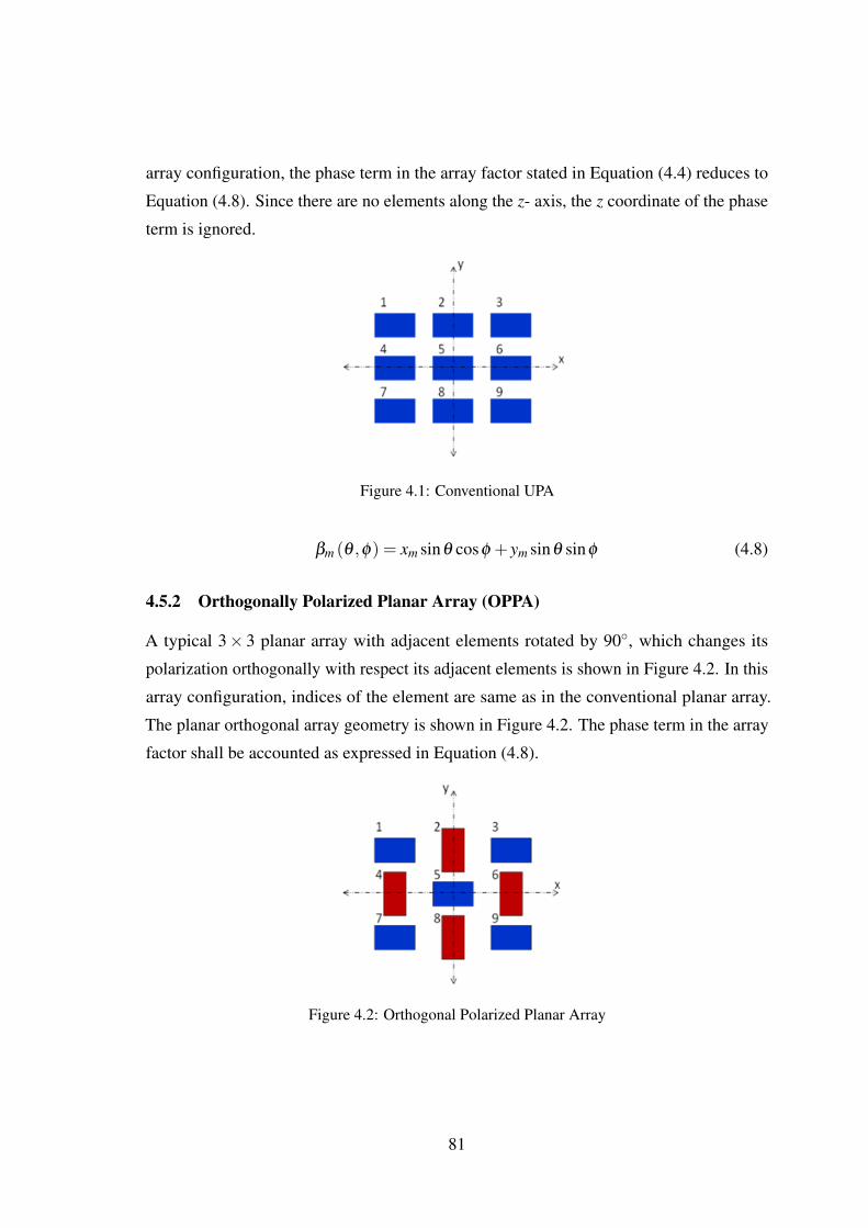
array configuration, the phase term in the array factor stated in Equation (4.4) reduces to
Equation (4.8). Since there are no elements along the z- axis, the z coordinate of the phase
term is ignored.
Figure 4.1: Conventional UPA
βm (θ ,φ) = xm sinθ cosφ + ym sinθ sinφ (4.8)
4.5.2 Orthogonally Polarized Planar Array (OPPA)
A typical 3× 3 planar array with adjacent elements rotated by 90◦, which changes its
polarization orthogonally with respect its adjacent elements is shown in Figure 4.2. In this
array configuration, indices of the element are same as in the conventional planar array.
The planar orthogonal array geometry is shown in Figure 4.2. The phase term in the array
factor shall be accounted as expressed in Equation (4.8).
Figure 4.2: Orthogonal Polarized Planar Array
81

4.5.3 Orthogonally Mounted Linear Array (OMLA)
The OMLA configuration also involves both vertical and horizontal polarized elements. As
shown in Figure 4.3, OMLA looks like a planar array. In the configuration of OMLA shown
in Figure 4.3, the horizontally polarized antenna element ’2’ is placed on the vertically
polarized antenna element ’1’ with no spacing between the edges of the mounted elements.
However, these two orthogonally polarized elements exhibit a spacing of (a+b)/2 (center
to center) along the y axis. There is a spacing along the x axis between successive like
polarized elements. In view of the presence of the spatial variations of the elements
along both x and y axes, the OMLA appears like a planar array. Since the size of array
configuration shown in Figure 4.3 can be increased with the additional elements along the
x axis only, this configuration tantamount to ’linear array’.
Figure 4.3: Orthogonal Mounted Linear Array
4.5.4 Orthogonally Polarized Linear Array (OPLA)
The classical linear array is modified to satisfy that adjacent elements are orthogonal to
each other. In this array configuration, the antenna elements are mounted along only one
axis (say x-axis). There is a the phase variation along the x-axis only. Thus the phase term
mentioned in Equation (4.4) reduces to Equation (4.9).
βm (θ ,φ) = xm sinθ cosφ (4.9)
The OPLA is shown in Figure 4.4. Unlike typical linear array geometries, this OPLA
configuration is capable of determining two dimensional DOA (both azimuth and elevation
angles).
82

Figure 4.4: Orthogonally Polarized Linear Array
4.6 Simulation Environment
The simulation environment is configured through the signal modelling of the conventional
uniform planar and proposed diversely polarized array configurations. As stated earlier
X-band rectangular waveguide is chosen as an antenna for the analysis. The standard
dimension of the X-band waveguide of width a = 2.32cm and height b = 1cm is consid-
ered. The RWG is operated at its T E10 dominant mode. The frequency and wavelength
of the simulation setup are 9.375 GHz and 3.2cm respectively. The standard spectral
MUSIC algorithm described in subsection 2.8.2.2 (Equations(2.32 and 3.7)) is used for
the computation of the 2D-DOA estimation for the conventional and proposed orthogonal
array configurations.
The elements of the array are oriented such that the array receives both the vertical and
horizontal polarized components independently at their respective elements. The signals of
opposite (orthogonal) polarization do not combine in space. However the samples received
from the vertical and horizontal polarized antenna elements are combined to produce the
spatial covariance matrix. The covariance between the vertical and horizontal polarized
signal components are utilized to improve the accuracy and angular resolution of the DOA,
when compared to the single polarized spatial covariance matrix of UPA.
4.7 Analysis of Accuracy of Estimation of 2D-DOA
The following simulation results illustrate the estimation accuracy of the proposed dual
polarized array configurations and its results are compared with the singly polarized UPA
configurations. The 2D-DOA estimation is analysed through the RMSE of the estimation
for the SNR range of 0 - 30 dB and averaged over 200 Monte-Carlo iterations. In the
comparison of estimation accuracy of 2D-DOA estimation, different array configurations
namely UPA, OPPA, OMLA and OPLA are used.
83
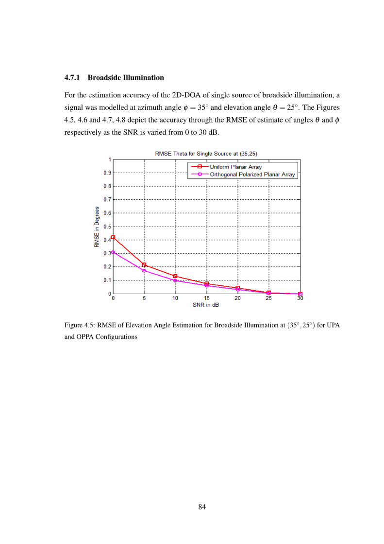
4.7.1 Broadside Illumination
For the estimation accuracy of the 2D-DOA of single source of broadside illumination, a
signal was modelled at azimuth angle φ = 35◦ and elevation angle θ = 25◦. The Figures
4.5, 4.6 and 4.7, 4.8 depict the accuracy through the RMSE of estimate of angles θ and φ
respectively as the SNR is varied from 0 to 30 dB.
Figure 4.5: RMSE of Elevation Angle Estimation for Broadside Illumination at (35◦,25◦) for UPA
and OPPA Configurations
84

Figure 4.6: RMSE of Elevation Angle Estimation for Broadside Illumination at (35◦,25◦) for
OMLA and OPLA Configurations
The results of RMSE of elevation angle θ of DOA estimation are shown in Figure 4.5
for UPA and OPPA as well as in Figure 4.6 for OMLA and OPLA. The results of Figures
4.5 and 4.6 illustrate that OPPA configuration exhibits least RMSE when compared to
the UPA, OMLA and OPLA configurations. At low SNR scenario (<10 dB) a relative
difference in RMSE is found to be (0.3◦- 0.4◦). At higher SNR, the relative difference in
RMSE is still smaller. The ability of OPPA to estimate the elevation angle θ of DOA with
least error is attributed to its elements which exhibit the spatial phase variation along x
and y axes. The elements of OMLA configuration experience the spatial phase variation
predominantly along x axis when compared to y axis and hence a small difference in
RMSE with respect to that of OPPA is present. The complete absence of spatial phase
variation along y axis leading to relatively higher increased RMSE can be seen in OPLA
configuration. In UPA configurations, the antenna elements experience spatial phase
variation along x and y axes. However, UPA configuration suffers from the absence of
orthogonal polarized antenna elements leading to a slightly more RMSE compared to
OPPA configuration. By comparing the planar array configurations for DOA estimation,
UPA and OPPA show a relative reduction of RMSE at lower SNRs .
85

Figure 4.7: RMSE of Azimuth Angle Estimation for Broadside Illumination at (35◦,25◦) for UPA
and OPPA Configurations
Figure 4.8: RMSE of Azimuth Angle Estimation for Broadside Illumination at (35◦,25◦) for OMLA
and OPLA Configurations
86
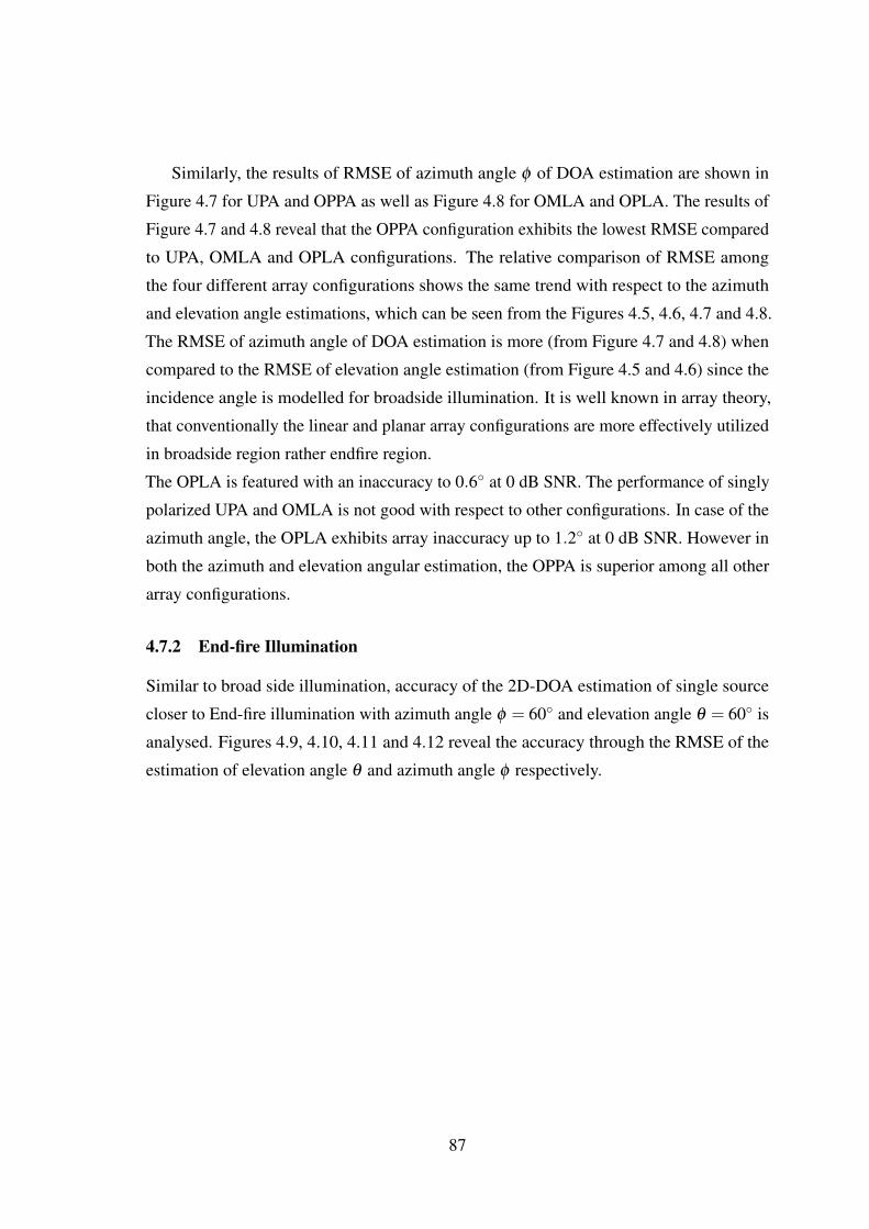
Similarly, the results of RMSE of azimuth angle φ of DOA estimation are shown in
Figure 4.7 for UPA and OPPA as well as Figure 4.8 for OMLA and OPLA. The results of
Figure 4.7 and 4.8 reveal that the OPPA configuration exhibits the lowest RMSE compared
to UPA, OMLA and OPLA configurations. The relative comparison of RMSE among
the four different array configurations shows the same trend with respect to the azimuth
and elevation angle estimations, which can be seen from the Figures 4.5, 4.6, 4.7 and 4.8.
The RMSE of azimuth angle of DOA estimation is more (from Figure 4.7 and 4.8) when
compared to the RMSE of elevation angle estimation (from Figure 4.5 and 4.6) since the
incidence angle is modelled for broadside illumination. It is well known in array theory,
that conventionally the linear and planar array configurations are more effectively utilized
in broadside region rather endfire region.
The OPLA is featured with an inaccuracy to 0.6◦ at 0 dB SNR. The performance of singly
polarized UPA and OMLA is not good with respect to other configurations. In case of the
azimuth angle, the OPLA exhibits array inaccuracy up to 1.2◦ at 0 dB SNR. However in
both the azimuth and elevation angular estimation, the OPPA is superior among all other
array configurations.
4.7.2 End-fire Illumination
Similar to broad side illumination, accuracy of the 2D-DOA estimation of single source
closer to End-fire illumination with azimuth angle φ = 60◦ and elevation angle θ = 60◦ is
analysed. Figures 4.9, 4.10, 4.11 and 4.12 reveal the accuracy through the RMSE of the
estimation of elevation angle θ and azimuth angle φ respectively.
87

Figure 4.9: RMSE of Elevation Angle Estimation for End-fire Illumination at (60◦,60◦) for UPA
and OPPA Configurations
Figure 4.10: RMSE of Elevation Angle Estimation for End-fire Illumination at (60◦,60◦) for OMLA
and OPLA Configurations
88
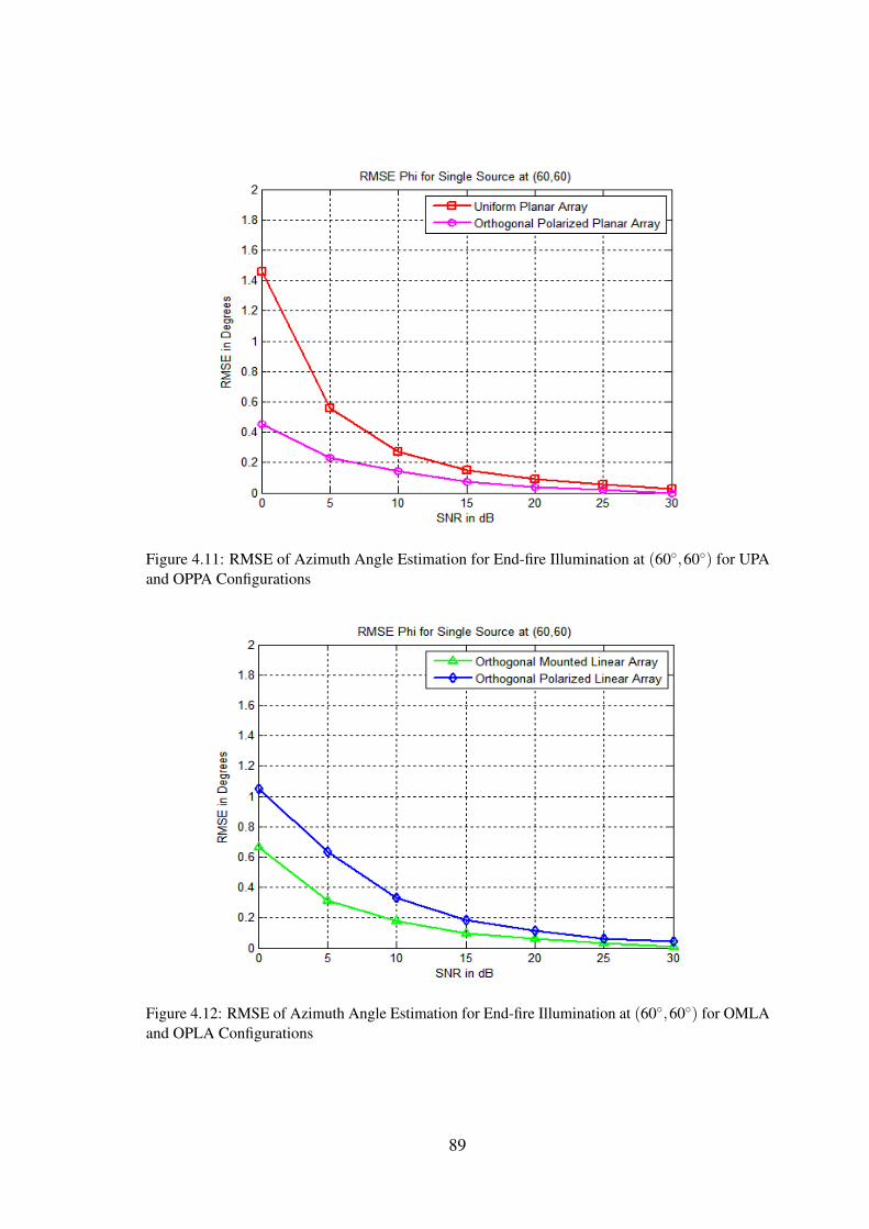
Figure 4.11: RMSE of Azimuth Angle Estimation for End-fire Illumination at (60◦,60◦) for UPAand OPPA Configurations
Figure 4.12: RMSE of Azimuth Angle Estimation for End-fire Illumination at (60◦,60◦) for OMLAand OPLA Configurations
89

The results of Figure 4.9 illustrate that a maximum error of 3.5◦ at SNR of 0 dB
for both UPA configuration and OPLA configuration. The OPPA achieves a minimum
RMSE of 0.8◦ at 0 dB. The OMLA exhibits a relatively poorer performance amongst
the array configurations. The RMSE of the azimuth angle ranges between 0.5◦ to 1.5◦
for the different array configurations. The conventional UPA exhibits error of 1.5◦ at
SNR of 0 dB and continues to perform similar to the OPLA configuration. The OMLA
configuration continues to exhibit average performance and the OPPA shows superior
performance among all other array configurations.
4.8 Discussion of Results on 2D-DOA of Single Source
The 2D-DOA estimations obtained through OPPA exhibit relatively better performance
over singly polarized UPA and also with OPLA, implying that, diversely polarized planar
array configuration is better than UPA configuration. From the simulation analysis it is also
evident that in 2D-DOA estimation, the angle of illumination of sources is also a factor
in the estimation accuracy provided the antenna element patterns are considered in the
analysis. From the analysis of broadside and end-fire illumination of signal sources, it is
shown that estimation accuracy depends on the region of illumination with respect to the
antenna geometry and antenna radiation pattern. In general, the broadside illumination has
lesser estimation error when compared to the end-fire illumination. When the azimuth and
elevation angles of DOA broadly fall into broadside illumination, the estimation accuracy
of elevation angle θ is greater than the source illuminated in end-fire region. This is due
to higher gain of the radiation pattern in the broadside region and progressively reduced
gain in the end-fire region. The accuracy of azimuth angle φ estimation is almost the same
irrespective region of illumination. However minor changes are seen in the accuracy due to
the spatial phase variations in the configuration. The RMSE of DOA estimation with OPLA
is more compared to the conventional singly polarized array due to the linear arrangement
of element of elements. The spatial phase variation only along the x axis is present in
OPLA configuration, where as spatial phase variations in the both x and y axes are seen in
the other array configuration. However it is evidently clear from the simulation analysis
that, the OPLA although a geometrically linear configuration is a potential candidate to
estimate 2D-DOA estimation. A conventional singly polarized linear array geometry is not
adequate for 2D-DOA estimation.
90

Figure 4.13: Two Dimensional DOA Estimation of Two Sources using UPA for 20 dB SNR
4.9 Analysis of 2D-DOA Estimation for Two Sources
After having established the validity of proposed array configurations for the 2D-DOA
estimation with a single source, simulation studies have been performed to substantiate
the performance of 2D-DOA estimation for two sources. The conventional UPA, OPPA,
OMLA and OPLA as indicated in the Figures 4.1, 4.2, 4.3 and 4.4 respectively are
considered for the analysis. The 2D-MUSIC algorithm is modelled for the various array
configurations for the 2D-DOA estimation. Modelling of the two sources with arriving
angles of (θ1 = 52◦,φ1 = 28◦) and (θ2 = 40◦,φ2 = 65◦) has been carried for the varying
SNR values of 20 dB, 10 dB and 0 dB. This analysis is carried out to compare the
distinguishing features of the estimation of DOA angles obtained with the various array
configurations.
4.9.1 Results of 2D-DOA of Two Sources at 20 dB SNR
In this subsection, a detailed analysis of the simulation results of 2D-DOA estimation with
two sources derived with various array configurations is presented. For the purpose of
simulation studies, signal modelling has been performed with 2D-DOA azimuthal and
elevation angles of two sources as (θ1 = 52◦,φ1 = 28◦) and (θ2 = 40◦,φ2 = 65◦).
91

Figure 4.13 illustrates the results of estimating 2D-DOA angles of two sources derived
with conventional UPA. There is a perfect match between the 2D-DOA angles assumed
in the signal modelling and the estimated angles derived through the MUSIC based DOA
estimation algorithm. The noticeable observation in the results of Figure 4.13 is the
presence of an additional peak whose magnitude is significantly lesser than the other two
peaks. Based on this inference, one can ignore it as a fictitious one.
The appearance of additional peak in the UPA configuration is due to larger inter-
element spacing between the array elements because of which there is an inadequacy of
spatial samples during one wavelength of the signal. This in turn leads to spatial aliasing
resulting in additional peak or peaks. The minimum inter-element spacing along the x axis
for UPA configuration itself is greater than the half of the wavelength (considering the
dimensions of X-band RWG as (2.32cmx1cm) at λ of 3.2cm corresponding to 9.375 GHz).
Assuming negligibly small wall thickness of the waveguide, the minimum inter-element
spacing along the x-axis is equal to 2.32cm, which is 0.725λ and along the y-axis it is 0.31λ .
In the case of OPPA, the minimum spacing between the successive elements along both x
and y axes is equal to 1.16 + 0.5 = 1.66 cm, which is equivalent to 0.518λ The inter-element
spacing much greater than λ/2 in the case of UPA is due to the physical aperture and
the geometrical arrangement of its elements. The orthogonal array configurations such as
Figure 4.14: Two Dimensional DOA Estimation of Two Sources using OPPA for 20 dB SNR
92
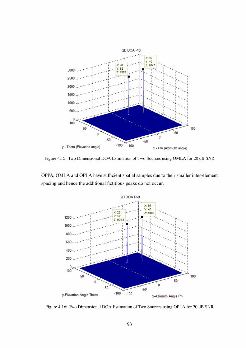
Figure 4.15: Two Dimensional DOA Estimation of Two Sources using OMLA for 20 dB SNR
OPPA, OMLA and OPLA have sufficient spatial samples due to their smaller inter-element
spacing and hence the additional fictitious peaks do not occur.
Figure 4.16: Two Dimensional DOA Estimation of Two Sources using OPLA for 20 dB SNR
93
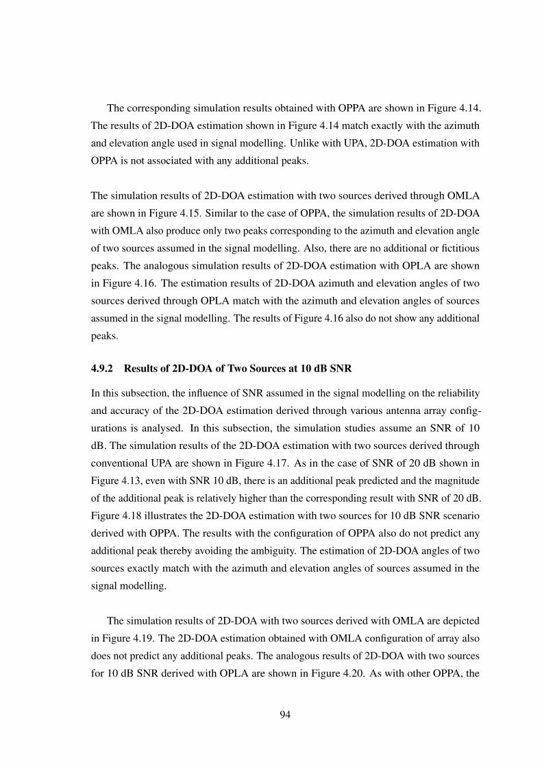
The corresponding simulation results obtained with OPPA are shown in Figure 4.14.
The results of 2D-DOA estimation shown in Figure 4.14 match exactly with the azimuth
and elevation angle used in signal modelling. Unlike with UPA, 2D-DOA estimation with
OPPA is not associated with any additional peaks.
The simulation results of 2D-DOA estimation with two sources derived through OMLA
are shown in Figure 4.15. Similar to the case of OPPA, the simulation results of 2D-DOA
with OMLA also produce only two peaks corresponding to the azimuth and elevation angle
of two sources assumed in the signal modelling. Also, there are no additional or fictitious
peaks. The analogous simulation results of 2D-DOA estimation with OPLA are shown
in Figure 4.16. The estimation results of 2D-DOA azimuth and elevation angles of two
sources derived through OPLA match with the azimuth and elevation angles of sources
assumed in the signal modelling. The results of Figure 4.16 also do not show any additional
peaks.
4.9.2 Results of 2D-DOA of Two Sources at 10 dB SNR
In this subsection, the influence of SNR assumed in the signal modelling on the reliability
and accuracy of the 2D-DOA estimation derived through various antenna array config-
urations is analysed. In this subsection, the simulation studies assume an SNR of 10
dB. The simulation results of the 2D-DOA estimation with two sources derived through
conventional UPA are shown in Figure 4.17. As in the case of SNR of 20 dB shown in
Figure 4.13, even with SNR 10 dB, there is an additional peak predicted and the magnitude
of the additional peak is relatively higher than the corresponding result with SNR of 20 dB.
Figure 4.18 illustrates the 2D-DOA estimation with two sources for 10 dB SNR scenario
derived with OPPA. The results with the configuration of OPPA also do not predict any
additional peak thereby avoiding the ambiguity. The estimation of 2D-DOA angles of two
sources exactly match with the azimuth and elevation angles of sources assumed in the
signal modelling.
The simulation results of 2D-DOA with two sources derived with OMLA are depicted
in Figure 4.19. The 2D-DOA estimation obtained with OMLA configuration of array also
does not predict any additional peaks. The analogous results of 2D-DOA with two sources
for 10 dB SNR derived with OPLA are shown in Figure 4.20. As with other OPPA, the
94
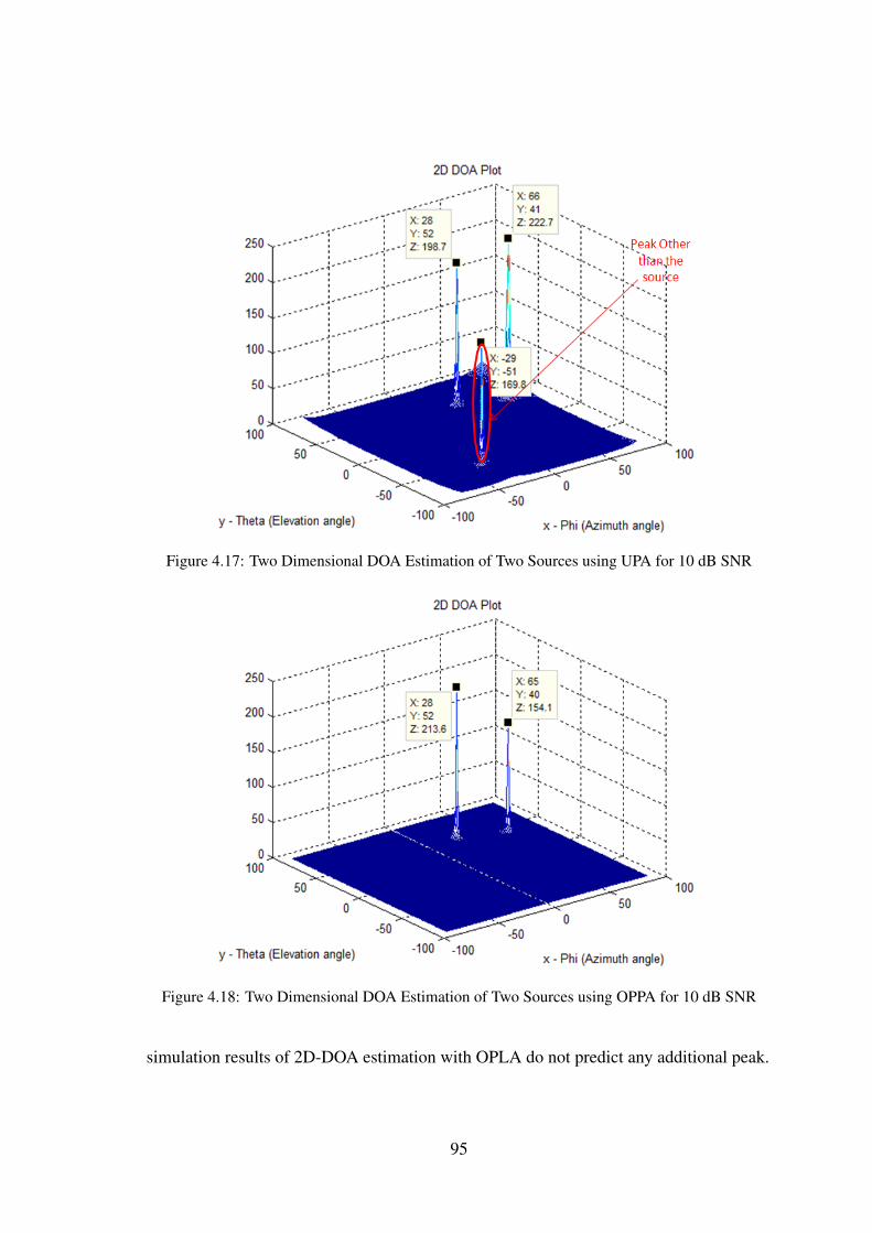
Figure 4.17: Two Dimensional DOA Estimation of Two Sources using UPA for 10 dB SNR
Figure 4.18: Two Dimensional DOA Estimation of Two Sources using OPPA for 10 dB SNR
simulation results of 2D-DOA estimation with OPLA do not predict any additional peak.
95

Figure 4.19: Two Dimensional DOA Estimation of Two Sources using OMLA for 10 dB SNR
Figure 4.20: Two Dimensional DOA Estimation of Two Sources using OPLA for 10 dB SNR
4.9.3 Results of 2D-DOA of Two Sources at 0 dB SNR
In this subsection, the simulation studies emphasise the influence of 0 dB SNR on the
accuracy of 2D-DOA estimation with two sources. A scenario of 0 dB SNR implies that
96
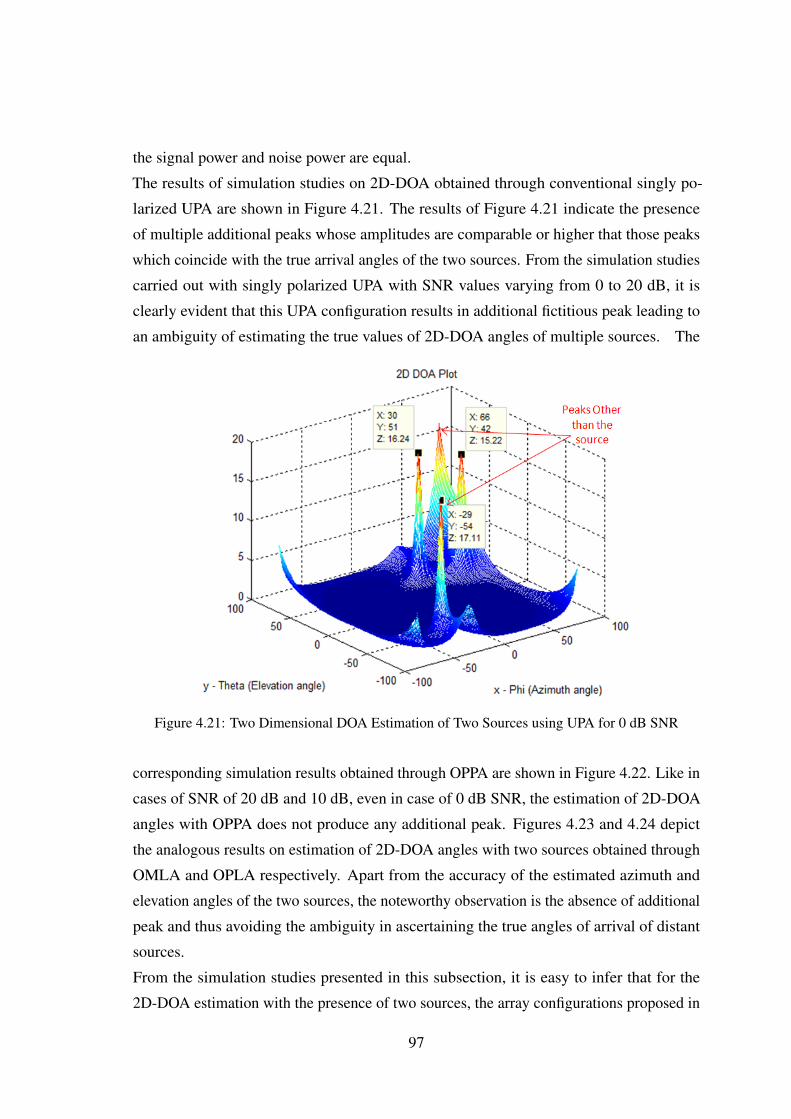
the signal power and noise power are equal.
The results of simulation studies on 2D-DOA obtained through conventional singly po-
larized UPA are shown in Figure 4.21. The results of Figure 4.21 indicate the presence
of multiple additional peaks whose amplitudes are comparable or higher that those peaks
which coincide with the true arrival angles of the two sources. From the simulation studies
carried out with singly polarized UPA with SNR values varying from 0 to 20 dB, it is
clearly evident that this UPA configuration results in additional fictitious peak leading to
an ambiguity of estimating the true values of 2D-DOA angles of multiple sources. The
Figure 4.21: Two Dimensional DOA Estimation of Two Sources using UPA for 0 dB SNR
corresponding simulation results obtained through OPPA are shown in Figure 4.22. Like in
cases of SNR of 20 dB and 10 dB, even in case of 0 dB SNR, the estimation of 2D-DOA
angles with OPPA does not produce any additional peak. Figures 4.23 and 4.24 depict
the analogous results on estimation of 2D-DOA angles with two sources obtained through
OMLA and OPLA respectively. Apart from the accuracy of the estimated azimuth and
elevation angles of the two sources, the noteworthy observation is the absence of additional
peak and thus avoiding the ambiguity in ascertaining the true angles of arrival of distant
sources.
From the simulation studies presented in this subsection, it is easy to infer that for the
2D-DOA estimation with the presence of two sources, the array configurations proposed in
97

Figure 4.22: Two Dimensional DOA Estimation of Two Sources using OPPA for 0 dB SNR
Figure 4.23: Two Dimensional DOA Estimation of Two Sources using OMLA for 0 dB SNR
the thesis that are featured with orthogonal polarization ensure relatively more accurate
results and they are also associated with the distinct feature of absence of fictitious peaks.
98
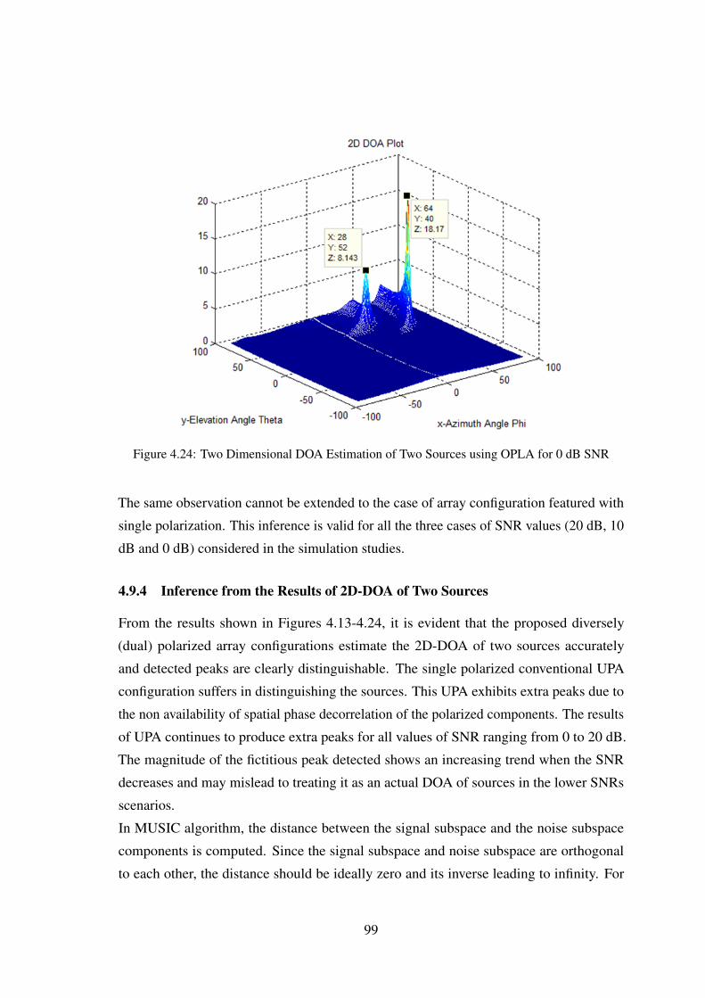
Figure 4.24: Two Dimensional DOA Estimation of Two Sources using OPLA for 0 dB SNR
The same observation cannot be extended to the case of array configuration featured with
single polarization. This inference is valid for all the three cases of SNR values (20 dB, 10
dB and 0 dB) considered in the simulation studies.
4.9.4 Inference from the Results of 2D-DOA of Two Sources
From the results shown in Figures 4.13-4.24, it is evident that the proposed diversely
(dual) polarized array configurations estimate the 2D-DOA of two sources accurately
and detected peaks are clearly distinguishable. The single polarized conventional UPA
configuration suffers in distinguishing the sources. This UPA exhibits extra peaks due to
the non availability of spatial phase decorrelation of the polarized components. The results
of UPA continues to produce extra peaks for all values of SNR ranging from 0 to 20 dB.
The magnitude of the fictitious peak detected shows an increasing trend when the SNR
decreases and may mislead to treating it as an actual DOA of sources in the lower SNRs
scenarios.
In MUSIC algorithm, the distance between the signal subspace and the noise subspace
components is computed. Since the signal subspace and noise subspace are orthogonal
to each other, the distance should be ideally zero and its inverse leading to infinity. For
99
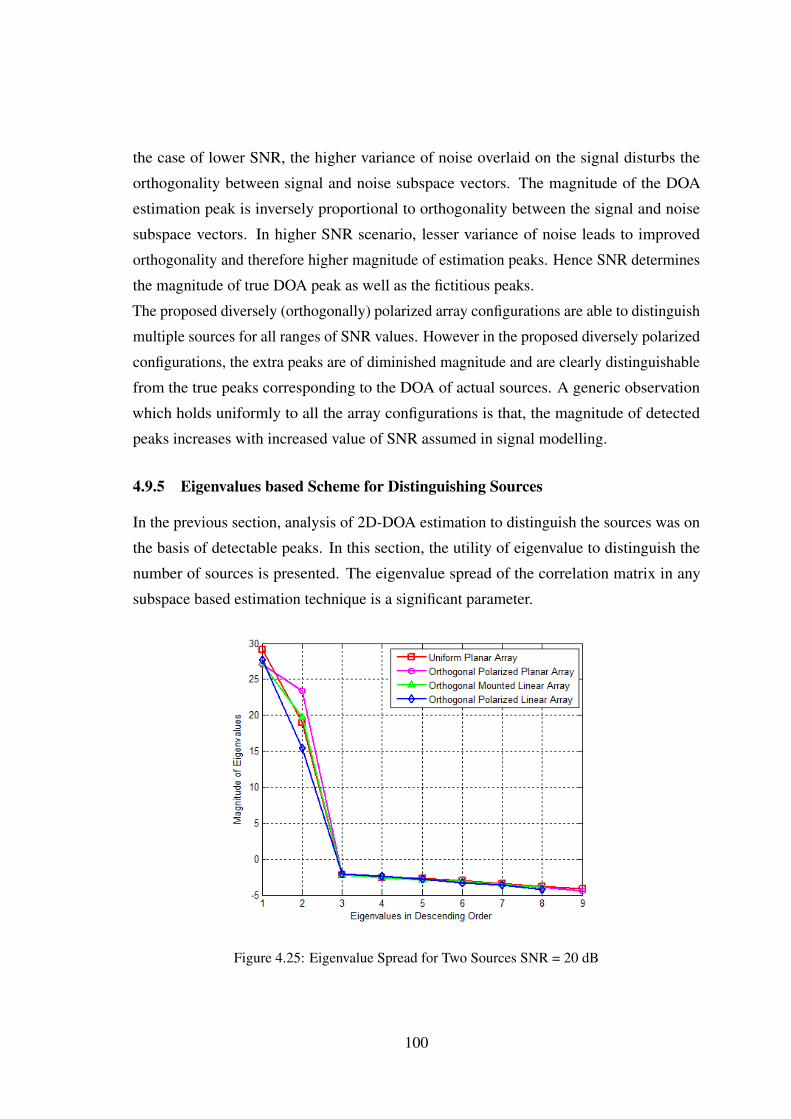
the case of lower SNR, the higher variance of noise overlaid on the signal disturbs the
orthogonality between signal and noise subspace vectors. The magnitude of the DOA
estimation peak is inversely proportional to orthogonality between the signal and noise
subspace vectors. In higher SNR scenario, lesser variance of noise leads to improved
orthogonality and therefore higher magnitude of estimation peaks. Hence SNR determines
the magnitude of true DOA peak as well as the fictitious peaks.
The proposed diversely (orthogonally) polarized array configurations are able to distinguish
multiple sources for all ranges of SNR values. However in the proposed diversely polarized
configurations, the extra peaks are of diminished magnitude and are clearly distinguishable
from the true peaks corresponding to the DOA of actual sources. A generic observation
which holds uniformly to all the array configurations is that, the magnitude of detected
peaks increases with increased value of SNR assumed in signal modelling.
4.9.5 Eigenvalues based Scheme for Distinguishing Sources
In the previous section, analysis of 2D-DOA estimation to distinguish the sources was on
the basis of detectable peaks. In this section, the utility of eigenvalue to distinguish the
number of sources is presented. The eigenvalue spread of the correlation matrix in any
subspace based estimation technique is a significant parameter.
Figure 4.25: Eigenvalue Spread for Two Sources SNR = 20 dB
100

The spread of the eigenvalues are analysed in 2D-DOA for the two sources at (θ1 =
52◦,φ1 = 28◦) and (θ2 = 40◦,φ2 = 65◦). The analysis is carried for the range of SNR
values like 20 dB, 10 dB, 5 dB and 0 dB. The eigenvalues are sorted in a descending order
and have been compared for the different array configurations.
Figure 4.26: Eigenvalue Spread for Two Sources SNR = 10 dB
101
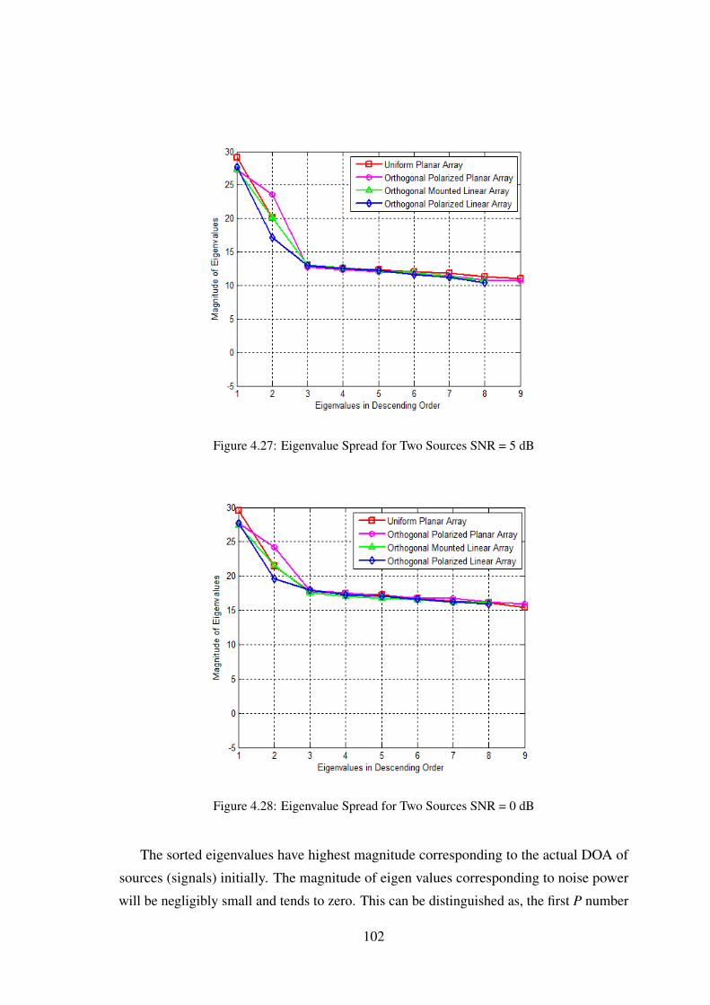
Figure 4.27: Eigenvalue Spread for Two Sources SNR = 5 dB
Figure 4.28: Eigenvalue Spread for Two Sources SNR = 0 dB
The sorted eigenvalues have highest magnitude corresponding to the actual DOA of
sources (signals) initially. The magnitude of eigen values corresponding to noise power
will be negligibly small and tends to zero. This can be distinguished as, the first P number
102
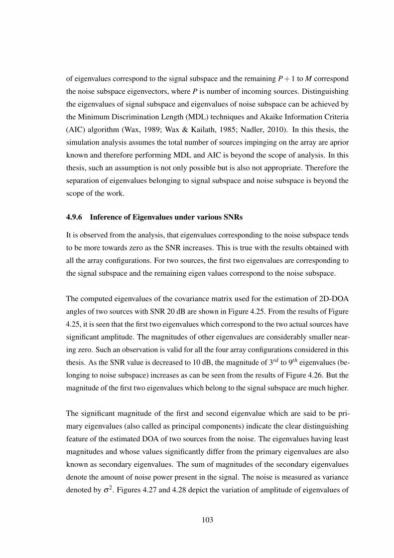
of eigenvalues correspond to the signal subspace and the remaining P+1 to M correspond
the noise subspace eigenvectors, where P is number of incoming sources. Distinguishing
the eigenvalues of signal subspace and eigenvalues of noise subspace can be achieved by
the Minimum Discrimination Length (MDL) techniques and Akaike Information Criteria
(AIC) algorithm (Wax, 1989; Wax & Kailath, 1985; Nadler, 2010). In this thesis, the
simulation analysis assumes the total number of sources impinging on the array are aprior
known and therefore performing MDL and AIC is beyond the scope of analysis. In this
thesis, such an assumption is not only possible but is also not appropriate. Therefore the
separation of eigenvalues belonging to signal subspace and noise subspace is beyond the
scope of the work.
4.9.6 Inference of Eigenvalues under various SNRs
It is observed from the analysis, that eigenvalues corresponding to the noise subspace tends
to be more towards zero as the SNR increases. This is true with the results obtained with
all the array configurations. For two sources, the first two eigenvalues are corresponding to
the signal subspace and the remaining eigen values correspond to the noise subspace.
The computed eigenvalues of the covariance matrix used for the estimation of 2D-DOA
angles of two sources with SNR 20 dB are shown in Figure 4.25. From the results of Figure
4.25, it is seen that the first two eigenvalues which correspond to the two actual sources have
significant amplitude. The magnitudes of other eigenvalues are considerably smaller near-
ing zero. Such an observation is valid for all the four array configurations considered in this
thesis. As the SNR value is decreased to 10 dB, the magnitude of 3rd to 9th eigenvalues (be-
longing to noise subspace) increases as can be seen from the results of Figure 4.26. But the
magnitude of the first two eigenvalues which belong to the signal subspace are much higher.
The significant magnitude of the first and second eigenvalue which are said to be pri-
mary eigenvalues (also called as principal components) indicate the clear distinguishing
feature of the estimated DOA of two sources from the noise. The eigenvalues having least
magnitudes and whose values significantly differ from the primary eigenvalues are also
known as secondary eigenvalues. The sum of magnitudes of the secondary eigenvalues
denote the amount of noise power present in the signal. The noise is measured as variance
denoted by σ2. Figures 4.27 and 4.28 depict the variation of amplitude of eigenvalues of
103
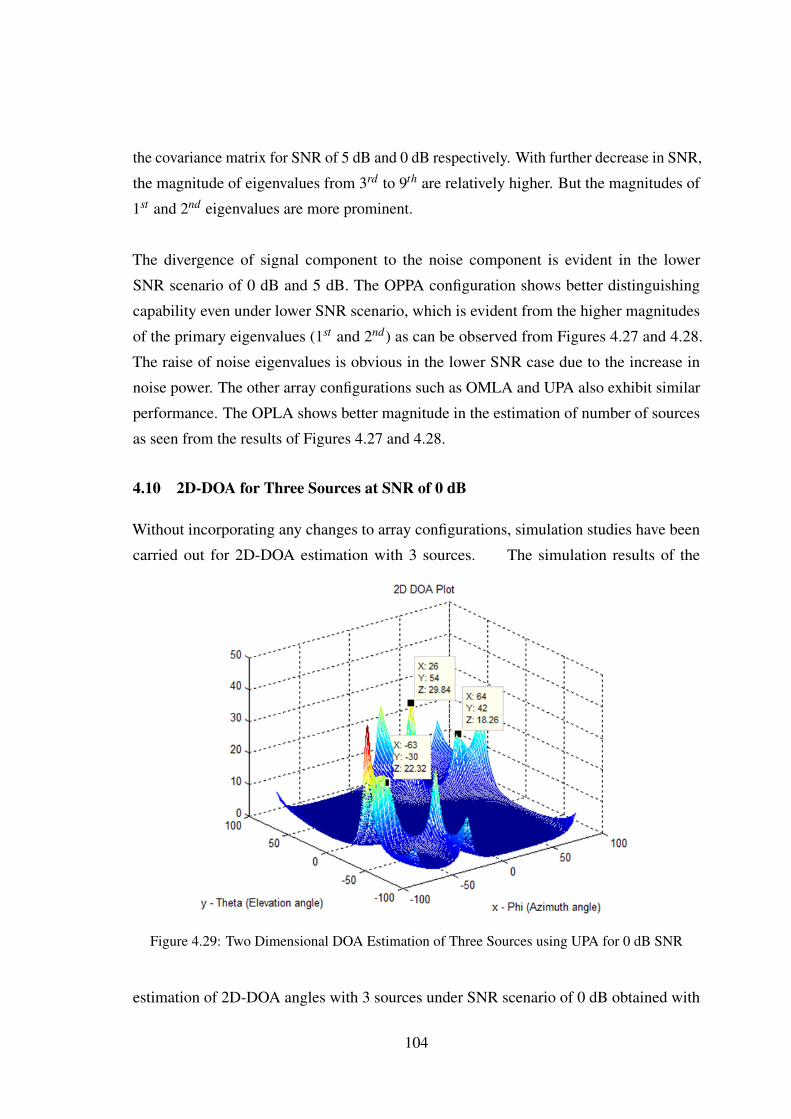
the covariance matrix for SNR of 5 dB and 0 dB respectively. With further decrease in SNR,
the magnitude of eigenvalues from 3rd to 9th are relatively higher. But the magnitudes of
1st and 2nd eigenvalues are more prominent.
The divergence of signal component to the noise component is evident in the lower
SNR scenario of 0 dB and 5 dB. The OPPA configuration shows better distinguishing
capability even under lower SNR scenario, which is evident from the higher magnitudes
of the primary eigenvalues (1st and 2nd) as can be observed from Figures 4.27 and 4.28.
The raise of noise eigenvalues is obvious in the lower SNR case due to the increase in
noise power. The other array configurations such as OMLA and UPA also exhibit similar
performance. The OPLA shows better magnitude in the estimation of number of sources
as seen from the results of Figures 4.27 and 4.28.
4.10 2D-DOA for Three Sources at SNR of 0 dB
Without incorporating any changes to array configurations, simulation studies have been
carried out for 2D-DOA estimation with 3 sources. The simulation results of the
Figure 4.29: Two Dimensional DOA Estimation of Three Sources using UPA for 0 dB SNR
estimation of 2D-DOA angles with 3 sources under SNR scenario of 0 dB obtained with
104
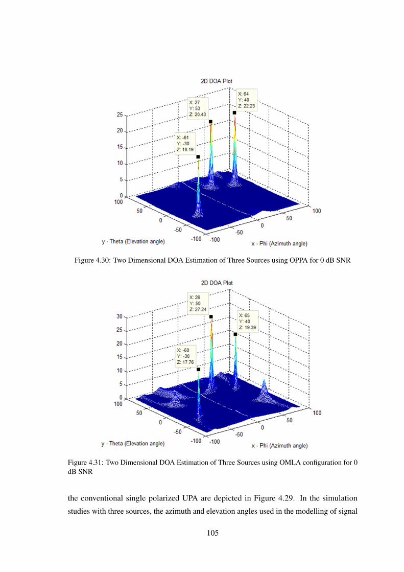
Figure 4.30: Two Dimensional DOA Estimation of Three Sources using OPPA for 0 dB SNR
Figure 4.31: Two Dimensional DOA Estimation of Three Sources using OMLA configuration for 0dB SNR
the conventional single polarized UPA are depicted in Figure 4.29. In the simulation
studies with three sources, the azimuth and elevation angles used in the modelling of signal
105

Figure 4.32: Two Dimensional DOA Estimation of Three Sources using OPLA for 0 dB SNR
impinging on the array configuration of DOA estimation system are (θ1 = 52◦,φ1 = 28◦),
(θ2 = 40◦,φ2 = 65◦) and (θ3 =−30◦,φ3 =−60◦).
As revealed by the results of Figure 4.29, the estimation of 2D-DOA with conventional
UPA is associated with numerous additional peaks which are fictitious. In addition, the
additional peaks which are supposed to have information on the DOA angles of true sources
have angular coordinates which are different from the ones used to simulate the impinging
signal.
The corresponding results derived through the OPPA are shown in Figure 4.30. As far the
cases with single and two sources, the estimation of 2D-DOA angles with three sources
using OPPA does not show any additional peaks thus avoiding the ambiguity. The estimated
2D-DOA angles of all the 3 sources are close to the ones assumed while modelling the
signal impinging on the OPPA.
The analogous results of 2D-DOA estimation with 3 sources under 0 dB SNR scenario
obtained with OMLA and OPLA are shown in Figures 4.31 and 4.32 respectively. The
results shown in Figure 4.31 and 4.32 are also not associated with additional peaks. The
estimated 2D-DOA angles of the three sources match closely with those assumed while
modelling the 3 sources.
106
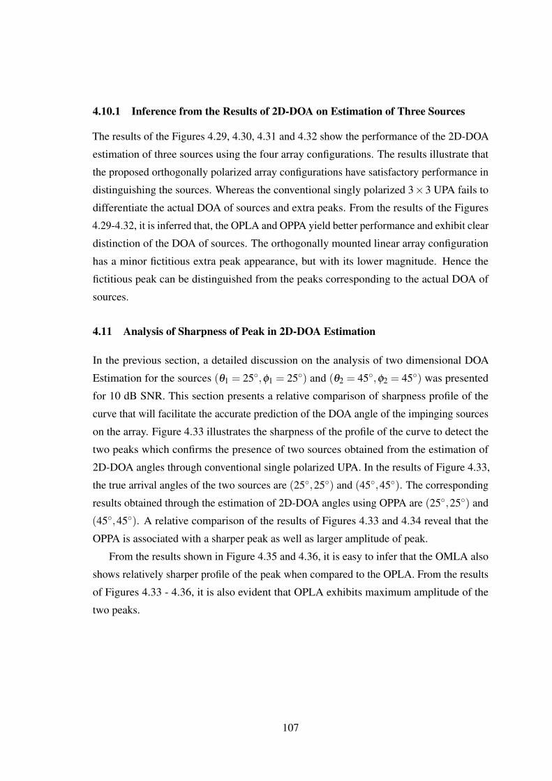
4.10.1 Inference from the Results of 2D-DOA on Estimation of Three Sources
The results of the Figures 4.29, 4.30, 4.31 and 4.32 show the performance of the 2D-DOA
estimation of three sources using the four array configurations. The results illustrate that
the proposed orthogonally polarized array configurations have satisfactory performance in
distinguishing the sources. Whereas the conventional singly polarized 3×3 UPA fails to
differentiate the actual DOA of sources and extra peaks. From the results of the Figures
4.29-4.32, it is inferred that, the OPLA and OPPA yield better performance and exhibit clear
distinction of the DOA of sources. The orthogonally mounted linear array configuration
has a minor fictitious extra peak appearance, but with its lower magnitude. Hence the
fictitious peak can be distinguished from the peaks corresponding to the actual DOA of
sources.
4.11 Analysis of Sharpness of Peak in 2D-DOA Estimation
In the previous section, a detailed discussion on the analysis of two dimensional DOA
Estimation for the sources (θ1 = 25◦,φ1 = 25◦) and (θ2 = 45◦,φ2 = 45◦) was presented
for 10 dB SNR. This section presents a relative comparison of sharpness profile of the
curve that will facilitate the accurate prediction of the DOA angle of the impinging sources
on the array. Figure 4.33 illustrates the sharpness of the profile of the curve to detect the
two peaks which confirms the presence of two sources obtained from the estimation of
2D-DOA angles through conventional single polarized UPA. In the results of Figure 4.33,
the true arrival angles of the two sources are (25◦,25◦) and (45◦,45◦). The corresponding
results obtained through the estimation of 2D-DOA angles using OPPA are (25◦,25◦) and
(45◦,45◦). A relative comparison of the results of Figures 4.33 and 4.34 reveal that the
OPPA is associated with a sharper peak as well as larger amplitude of peak.
From the results shown in Figure 4.35 and 4.36, it is easy to infer that the OMLA also
shows relatively sharper profile of the peak when compared to the OPLA. From the results
of Figures 4.33 - 4.36, it is also evident that OPLA exhibits maximum amplitude of the
two peaks.
107

Figure 4.33: 2D-DOA Estimation using UPA Configuration for Two Sources at (25◦,25◦) and(45◦,45◦) for SNR of 10dB
Figure 4.34: 2D-DOA Estimation using OPPA Configuration for Two Sources at (25◦,25◦) and(45◦,45◦) for SNR of 10dB
108
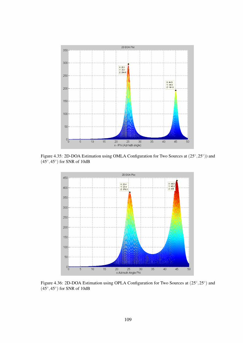
Figure 4.35: 2D-DOA Estimation using OMLA Configuration for Two Sources at (25◦,25◦)) and(45◦,45◦) for SNR of 10dB
Figure 4.36: 2D-DOA Estimation using OPLA Configuration for Two Sources at (25◦,25◦) and(45◦,45◦) for SNR of 10dB
109

4.12 Resolution Analysis of 2D-DOA Estimation with Closely Spaced Two Sources
A principal focus of this thesis is to formulate and analyse the schemes for improved
resolution and accuracy of estimation of 2D-DOA. A measure of resolvability of 2D-DOA
estimation algorithm is the ability of the algorithm to distinguish the peaks even when the
angular separation between the sources impinging on the array configuration is small. This
section presents the simulation results pertaining to the resolvability of the MUSIC based
2D-DOA estimation using various array configurations described earlier in this chapter.
The detection of the peaks resulting from the MUSIC algorithms based 2D-DOA estimation
techniques usually involves a visualization of 3D graph. To illustrate the ability of MUSIC
algorithm based 2D-DOA estimation technique to resolve closely spaced sources, a 2D
representation is preferred, in which 3D graph is viewed in 2D perspectives.
4.12.1 Analysis of 2D-DOA Estimation of Closely Spaced Two Sources using UPA
The results of the 2D-DOA estimation using UPA configuration are shown in Figures 4.37,
4.38 and 4.39. For the simulations, the two sources are modelled with the arrival angles of
(θ1 = 25◦,φ1 = 25◦) and (θ2 = 25◦,φ2 = 35◦).
Figure 4.37: 2D-DOA Estimation of Closely Spaced Sources Estimation using UPA for Two
Sources at (25◦,25◦) and (25◦,35◦)
110
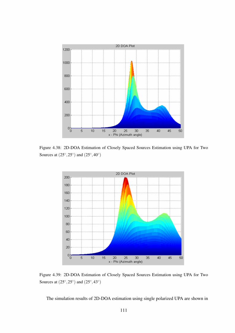
Figure 4.38: 2D-DOA Estimation of Closely Spaced Sources Estimation using UPA for Two
Sources at (25◦,25◦) and (25◦,40◦)
Figure 4.39: 2D-DOA Estimation of Closely Spaced Sources Estimation using UPA for Two
Sources at (25◦,25◦) and (25◦,43◦)
The simulation results of 2D-DOA estimation using single polarized UPA are shown in
111
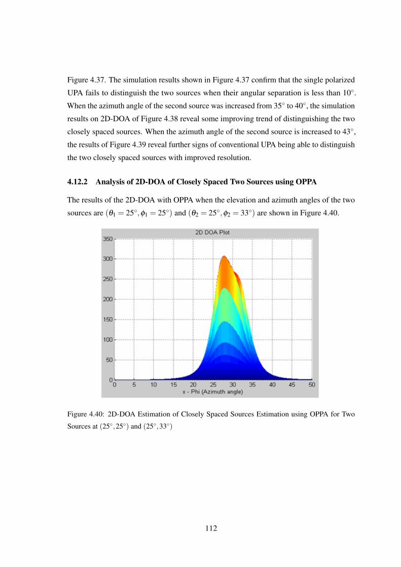
Figure 4.37. The simulation results shown in Figure 4.37 confirm that the single polarized
UPA fails to distinguish the two sources when their angular separation is less than 10◦.
When the azimuth angle of the second source was increased from 35◦ to 40◦, the simulation
results on 2D-DOA of Figure 4.38 reveal some improving trend of distinguishing the two
closely spaced sources. When the azimuth angle of the second source is increased to 43◦,
the results of Figure 4.39 reveal further signs of conventional UPA being able to distinguish
the two closely spaced sources with improved resolution.
4.12.2 Analysis of 2D-DOA of Closely Spaced Two Sources using OPPA
The results of the 2D-DOA with OPPA when the elevation and azimuth angles of the two
sources are (θ1 = 25◦,φ1 = 25◦) and (θ2 = 25◦,φ2 = 33◦) are shown in Figure 4.40.
Figure 4.40: 2D-DOA Estimation of Closely Spaced Sources Estimation using OPPA for Two
Sources at (25◦,25◦) and (25◦,33◦)
112

Figure 4.41: 2D-DOA Estimation of Closely Spaced Sources Estimation using OPPA for Two
Sources at (25◦,25◦) and (25◦,35◦)
As far the case of single polarized UPA configuration, the OPPA is not able to distin-
guish the two sources when the azimuth angles of the two sources differ by less than 10◦.
However, when the azimuth angle φ2 of the second source is changed to 35◦, the OPPA is
able to distinguish the two sources distinctly as can be inferred from the results of Figure
4.41. This is contrary to case the of conventional single polarized UPA.
4.12.3 Analysis of 2D-DOA Estimation of Closely Spaced Two Sources using OMLA
The results of Figure 4.42 reveal that the OMLA is not able to distinguish the two sources
whose elevation and azimuth angles of the two sources are (θ1 = 25◦,φ1 = 25◦) and
(θ2 = 25◦,φ2 = 33◦). When the azimuth angle φ2 of the second source is increased to 34◦
also, the OMLA is not able to distinguish the two sources as revealed by the results of
Figure 4.43. However, when the angle φ2 is changed to 35◦, the OMLA shows its ability to
infer the presence of two sources even though not with a distinctly visible second peak.
113

Figure 4.42: 2D-DOA Estimation of Closely Spaced Sources Estimation using OMLA for Two
Sources at (25◦,25◦) and (25◦,33◦)
Figure 4.43: 2D-DOA Estimation of Closely Spaced Sources Estimation using OMLA for Two
Sources at (25◦,25◦) and (25◦,34◦)
114
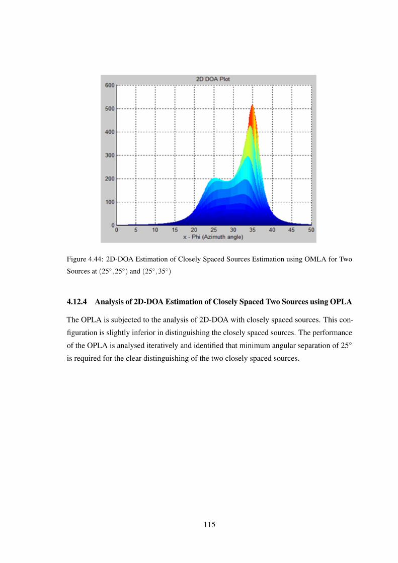
Figure 4.44: 2D-DOA Estimation of Closely Spaced Sources Estimation using OMLA for Two
Sources at (25◦,25◦) and (25◦,35◦)
4.12.4 Analysis of 2D-DOA Estimation of Closely Spaced Two Sources using OPLA
The OPLA is subjected to the analysis of 2D-DOA with closely spaced sources. This con-
figuration is slightly inferior in distinguishing the closely spaced sources. The performance
of the OPLA is analysed iteratively and identified that minimum angular separation of 25◦
is required for the clear distinguishing of the two closely spaced sources.
115
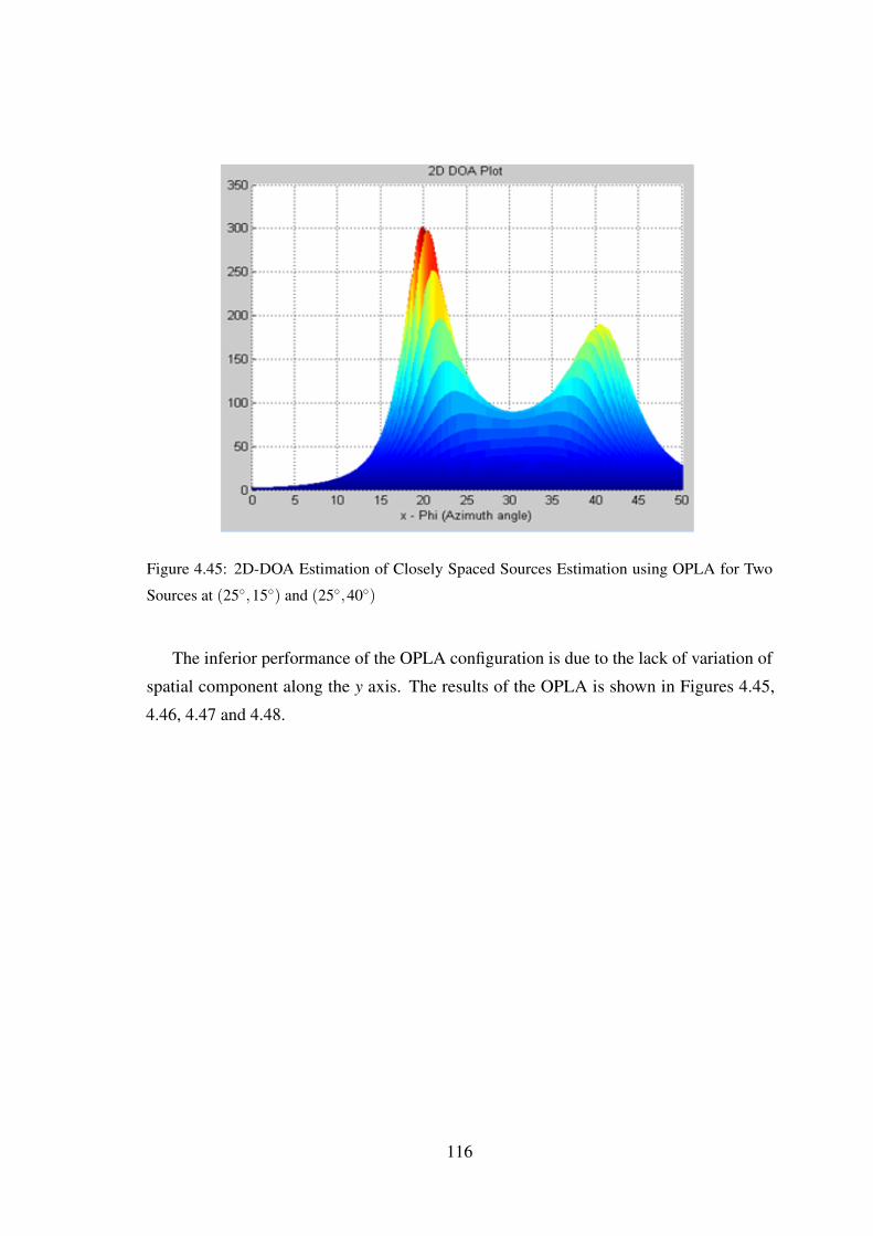
Figure 4.45: 2D-DOA Estimation of Closely Spaced Sources Estimation using OPLA for Two
Sources at (25◦,15◦) and (25◦,40◦)
The inferior performance of the OPLA configuration is due to the lack of variation of
spatial component along the y axis. The results of the OPLA is shown in Figures 4.45,
4.46, 4.47 and 4.48.
116

Figure 4.46: 2D-DOA Estimation of Closely Spaced Sources Estimation using OPLA for Two
Sources at (25◦,20◦) and (25◦,40◦)
Figure 4.47: 2D-DOA Estimation of Closely Spaced Sources Estimation using OPLA for Two
Sources at (25◦,25◦) and (15◦,45◦)
117

Figure 4.48: Closely Spaced Sources Estimation using OPLA for Two Sources at (25◦,25◦) and
(25◦,40◦)
4.13 Analysis of Effect of Inter Element Spacing on the 2D-DOA Estimation Per-formance
In this section, the influence of the inter element spacing of OPLA on the accuracy and
performance of 2D-DOA estimation algorithm is presented. Among the orthogonally
polarized array configurations, it is evident that the resolution and accuracy of 2D-DOA
estimation realized with OPLA has been relatively poor. In an attempt to analyse the
scheme for the performance enhancement of 2D-DOA estimation using OPLA, studies
have been carried out to analyse the effect of change in the inter element spacing on
the derived 2D-DOA estimation. As was stated in the section, in all the simulation
studies presented so far in this chapter, the inter element spacing is λ/4 at the operating
frequency of 9.375 GHz. The OPLA geometry was modified by doubling the inter element
spacing implying that the earlier value of 5.56 cm has been changed to 11.2 cm. With
the specific change, the simulation has been repeated for the estimation of 2D-DOA of
the two sources whose angular coordinates of impinging on the array elements of OPLA
are (θ1 = 25◦,φ1 = 25◦) and (θ2 = 25◦,φ2 = 35◦). Typically the inter element spacing is
optimized to achieve the better performance of DOA estimators where antenna elements
118
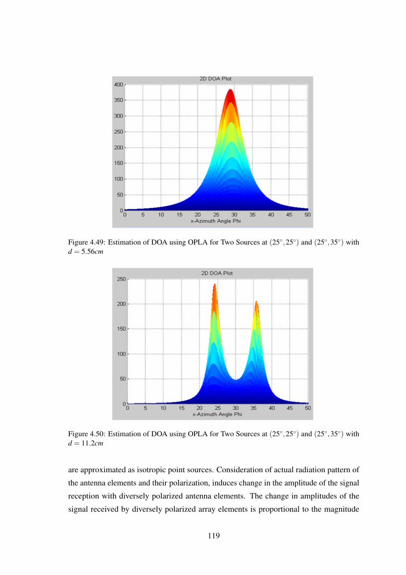
Figure 4.49: Estimation of DOA using OPLA for Two Sources at (25◦,25◦) and (25◦,35◦) withd = 5.56cm
Figure 4.50: Estimation of DOA using OPLA for Two Sources at (25◦,25◦) and (25◦,35◦) withd = 11.2cm
are approximated as isotropic point sources. Consideration of actual radiation pattern of
the antenna elements and their polarization, induces change in the amplitude of the signal
reception with diversely polarized antenna elements. The change in amplitudes of the
signal received by diversely polarized array elements is proportional to the magnitude
119

of radiation at that particular angle of incidence (DOA). Increased inter-element spacing
approximating to half the wavelength leads to improved covariance of the received samples.
This improvement in the covariance improves the DOA estimation.
The simulation results of 2D-DOA with increased inter elemental spacing using OPLA are
shown in Figure 4.50. A comparison of results of Figure 4.50 with the results of Figure 4.49
clearly demonstrates that the larger inter elemental spacing has significantly improved the
resolution of 2D-DOA results. The simulation results on estimation of 2D-DOA with the
angular coordinate of the two sources being (θ1 = 25◦,φ1 = 25◦) and (θ2 = 25◦,φ2 = 35◦)
derived through OPLA with d = 11.2 cm are shown in Figure 4.50. A comparison of
results of Figure 4.49 with Figure 4.50 confirms that the sharpness of the peaks of 2D-DOA
estimation improves with increased inter element spacing.
4.14 Summary
The simulations and analysis presented in this chapter confirm that the orthogonally polar-
ized components of antenna array have significant influence in the accuracy and resolution
of the 2D-DOA estimations. The proposed OPLA can be treated as an linear array. Thus
a linear array configuration and its ability to estimate 2D-DOA is the novel part of the
proposed OPLA. Among the proposed array configurations, OPPA has improved estimation
accuracy and the OMLA configuration estimates the two sources with higher magnitude.
The improved distinguishing capability of the OPPA for closely spaced sources is also
realized through the simulations. The OPPA and the OMLA configuration clearly distin-
guish the sources with minimum angular separation of 10◦ with accurate estimation. The
conventional single polarized UPA configuration resolves the 18◦ angular separation of
sources which is inferior when compared with the proposed OPPA and OMLA configura-
tions. The OPLA can resolve 10◦ angularly separated sources at the expense of increased
inter-element spacing. The improved estimation accuracy and resolution of the proposed
orthogonally polarized array configurations than the conventional single polarized UPA are
realized for 2D-DOA for two sources and three sources under high and low SNR (weak
coverage) conditions.
120

Chapter 5
Two Dimensional DOA Tracking of Non-Stationary Sources using
Subspace Tracking Algorithms
5.1 Introduction
High resolution subspace based parameter estimation algorithms are widely applied in
both temporal and spatial domain spectral analysis. Typical subspace based parameter
estimation algorithms highly rely on the statistical stationary characteristics of the sampled
received signal. Hence, the sample covariance data matrix obtained from the data samples
observed over a period is adequate for the parameter estimation. In case of a dynamic
scenario, where the moving signal sources have non-stationary signal characteristics, direct
application of the subspace estimation algorithm warrants repeated eigen decompositions
of the continuously updating data covariance matrix. In time varying systems, there will be
a more frequent change in vector sequence with time. Also there may be significant overlap
between new and old vector sequences. This warrants an analysis for the development of
adaptive eigen decomposition and subspace tracking algorithms discussed in Chapter 2.
This chapter intends to provide the simulation study on the analysis of tracking of 2D-DOA
of non-stationary signal sources. The simulation study includes novel method of smoothing
the covariance matrix of time varying non-stationary signal sources. The performance
analysis of tracking of 2D-DOA estimation is evaluated for the single polarized UPA and
the proposed orthogonal polarized array configurations for the range of SNR scenarios.
5.1.1 Adaptive Eigen Decomposition Algorithms
The adaptive eigen decomposition algorithm emerged in late 1970s, to avoid the repeated
computation of intensive eigen decomposition of the covariance matrix. Many research
contributions are reported in the literature for efficient updating and tracking of the subspace
components of the covariance matrix. For every new sample, these algorithms attempt
to recursively update the subspaces of eigen decomposition to avoid recomputing. A
121
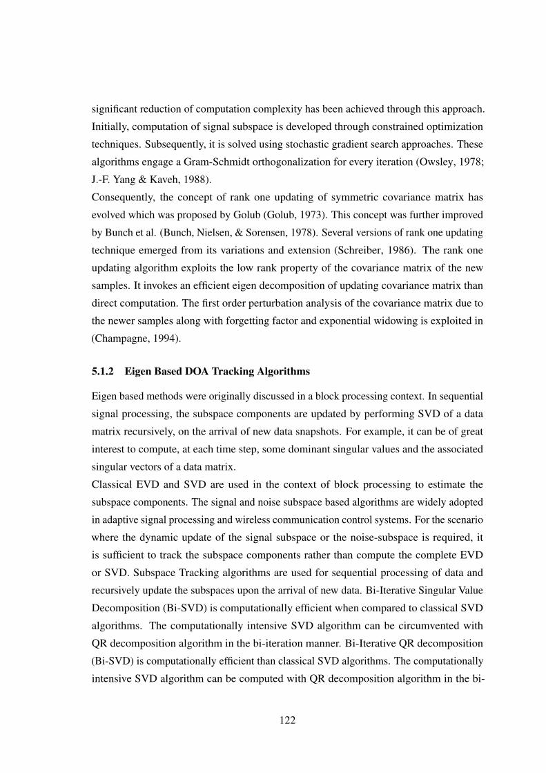
significant reduction of computation complexity has been achieved through this approach.
Initially, computation of signal subspace is developed through constrained optimization
techniques. Subsequently, it is solved using stochastic gradient search approaches. These
algorithms engage a Gram-Schmidt orthogonalization for every iteration (Owsley, 1978;
J.-F. Yang & Kaveh, 1988).
Consequently, the concept of rank one updating of symmetric covariance matrix has
evolved which was proposed by Golub (Golub, 1973). This concept was further improved
by Bunch et al. (Bunch, Nielsen, & Sorensen, 1978). Several versions of rank one updating
technique emerged from its variations and extension (Schreiber, 1986). The rank one
updating algorithm exploits the low rank property of the covariance matrix of the new
samples. It invokes an efficient eigen decomposition of updating covariance matrix than
direct computation. The first order perturbation analysis of the covariance matrix due to
the newer samples along with forgetting factor and exponential widowing is exploited in
(Champagne, 1994).
5.1.2 Eigen Based DOA Tracking Algorithms
Eigen based methods were originally discussed in a block processing context. In sequential
signal processing, the subspace components are updated by performing SVD of a data
matrix recursively, on the arrival of new data snapshots. For example, it can be of great
interest to compute, at each time step, some dominant singular values and the associated
singular vectors of a data matrix.
Classical EVD and SVD are used in the context of block processing to estimate the
subspace components. The signal and noise subspace based algorithms are widely adopted
in adaptive signal processing and wireless communication control systems. For the scenario
where the dynamic update of the signal subspace or the noise-subspace is required, it
is sufficient to track the subspace components rather than compute the complete EVD
or SVD. Subspace Tracking algorithms are used for sequential processing of data and
recursively update the subspaces upon the arrival of new data. Bi-Iterative Singular Value
Decomposition (Bi-SVD) is computationally efficient when compared to classical SVD
algorithms. The computationally intensive SVD algorithm can be circumvented with
QR decomposition algorithm in the bi-iteration manner. Bi-Iterative QR decomposition
(Bi-SVD) is computationally efficient than classical SVD algorithms. The computationally
intensive SVD algorithm can be computed with QR decomposition algorithm in the bi-
122

iteration manner. The subspace tracking algorithm Bi-SVD is detailed below. Many
variations of the Bi-SVD algorithm cited in the [Strobach 1997] literature with different
MACs of slow, fast and ultra fast.
5.1.3 Bi-SVD Algorithm
The Bi-SVD algorithm involves Bi-iteration of QR decomposition of the covariance matrix.
This bi-iteration simplifies the computation of the left and right singular vectors of the
classical SVD techniques. The steps to execute Bi-SVD algorithm are detailed in the
following pseudo code to decompose the covariance matrix Φ with r principal components.
Pseudo code of Bi-SVD
i. Initialize QA =
[Ir
0
]; where Ir is the identity matrix of size r× r and r is the number
of signal sources.
ii. f or i = 1, ...,until convergence
Bi = ΦiQA(i−1)
QBiRBi = QR(Bi)
Ai = ΦHi QBi
QAiRAi = QR(Ai)
end
Here QR(.) denotes the QR Decomposition of the matrix and (.)H refers to hermitian
conjugate.
The step (ii.) is iterated until convergence, and after convergence the left and right singular
vectors are settled in the B and A matrices respectively.
while the matrix Bi Settles for left dominant singular vectors, the matrix Ai Settles for right
dominant singular vectors
In mathematical sense, the r dominant singular vectors are equivalent to r signal subspace
vectors of eigen decomposition. Also the matrices Bi and Ai have the non-dominant
singular vectors, which are equivalent of noise subspace of the eigen decomposition. The
signal subspace based estimation algorithm requires to compute the dominant singular
vectors. Where as the noise subspace based algorithm warrants the non-dominant singular
vectors. Typically the signal subspace is associated with the principal components of the
123

covariance matrix, and noise subspace is associated with the non-principal components of
the covariance matrix. The Bi-SVD algorithm converges for the dominant singular vectors
first and later for the non-dominant vectors. The computationally intensive SVD algorithm
can be circumvented with QR decomposition algorithm in the bi-iteration manner such as
Bi-SVD and its variants.
5.2 Modelling of Signal Sources for Tracking of 2D-DOA
In DOA estimation, the data matrix or covariance matrix is processed for parameter
estimation using either MUSIC or ESPRIT based algorithms, in which computationally
intensive EVD or SVD technique are a routine must.
5.2.1 Modelling of Stationary Source
In case of the stationary sources, the array steering vector is fixed for all the samples and is
independent of the time index n as shown in Equation (5.1). In other words, the azimuth
(φ ) and elevation (θ ) angles are fixed for all the received samples of the array. The noise
added to the signal model is white Gaussian noise of fixed variance for all the time samples.
a(θ ,φ) =[e− jkβ1(θ ,φ), e− jkβ2(θ ,φ), · · · , e− jkβM(θ ,φ)
]T(5.1)
where,
βm (θ ,φ) = xm sinθ cosφ + ym sinθ sinφ + zm cosθ (5.2)
The standard array signal model for stationary sources are shown in Equation (5.3).
x(n) = a(θ ,φ)s(n)+w(n) (5.3)
where, x(n) is the received sample at time instant n. s(n) signal sample at instant n. w(n)
is the white Gaussian noise vector at instant n. The sample covariance matrix, Rxx is a
simple computation as shown in Equation (5.4).
Rxx = E[xxH] (5.4)
where (.)H refers to Hermitian conjugate.
124
5.2.2 Modelling of Non-stationary Source
In the case of non-stationary sources, the array steering vector is a function of time index
n. The azimuth and elevation angles of the incoming signal sources change over time
samples. The change in azimuth and elevation angles lead to change in phase of the
received samples in the observation interval. Thus, it is essential to compute the covariance
matrix independently for all the spatio-temporal samples. The time-varying source or
non-stationary source or dynamic source model is shown in Equation (5.5).
x(n) = a(θ ,φ ,n)s(n)+w(n) (5.5)
The covariance matrix is computed independently for all values of the time sample indices
n.
Rxx(n) = x(n)xH(n) (5.6)
The covariance matrices of instantaneous samples are computed in which the variance of
the spatial samples is not retained over the successive received samples, due to the dynamic
behaviour of the incoming sources. Retaining the second order statistical properties of
the received signal over the observation interval is essential for the better estimation of
the DOA. Various methods for the construction of covariance matrix are discussed in the
following subsections.
5.2.3 Covariance Matrix by Weighting Factor α
The concept of weighting factor based covariance computation widely used in adaptive
signal processing algorithms is utilized to retain the statistical properties of the incoming
sources. The weighting factor approach is formulated based on the typical moving average
filter (Hayes, 2009) and weighted average covariance matrix used in (Strobach, 1997). In
the weighting factor approach, the current sample along with the immediate past sample
are weighted, such that more weightage is for the current sample and less weightage for
the previous sample. In this method, covariance matrix for nth instant is computed by
RWxx(n) = (1−α)Rxx(n−1)+αRxx(n) (5.7)
where α is chosen such that 12 ≤ α ≤ 1.
The weighted averaged covariance matrix used for DOA estimation carries the statistical
properties of the signal from the beginning till the end. This in turn improves the DOA
estimation of the non-stationary sources. The weighting factor based covariance matrix is
shown in Equation (5.7)
125
5.2.4 Forgetting Factor β Method for Covariance Matrix
Similar to the weighting factor approach, concept of forgetting factor is introduced for the
dynamic source models. The forgetting factor technique is widely adopted in RLS type of
adaptive algorithms (S. S. Haykin, 2008). The concept of forgetting factor is to forget the
older samples in the memory. The size of the memory is fixed, keeping in view the ease of
the computation. It also depends on the dynamic behaviour of the source. In essence, it
can be said as the weighted sum of moving average filter. The covariance method Rffxx(n)
through the forgetting factor method is represented through the Equation (5.8).
Rffxx(n) =q
∑i=0
βiRxx(n− i) (5.8)
where β is chosen such that 0≤ β ≤ 1.
The β and q are respectively the forgetting factor and the order of the filter. This approach
carries the statistical property of the signal from the beginning more precisely than the
weighting factor approach. The forgetting factor based covariance matrix is shown in
Equation (5.8).
5.3 Simulation Analysis of DOA of Non-Stationary Sources
The simulation and performance analysis of DOA estimation are carried for the non-
stationary moving sources utilizing the instantaneous samples, weighting factor and forget-
ting factor approaches on the covariance matrix computations.
5.3.1 Tracking of DOA with MUSIC Algorithm
For the tracking of non-stationary sources, the standard MUSIC algorithm is incorporated to
estimate the DOA. The Root MUSIC algorithm can also be incorporated, which is variation
of the standard spectral MUSIC algorithm, in which polynomial rooting approach is
incorporated. The polynomial roots determined from the subspace components are utilized
to estimate the DOA. However, the Root MUSIC algorithm has the limitation of array
geometric configuration restricted to linear. The dynamic tracking of the moving sources
involves, the decomposition of signal and noise subspace components. The classical EVD
or SVD approaches intensify the computation over the observation interval. It is sufficient
to track the subspace components of the moving sources. The methods incorporated
involving weighting factor approach and forgetting factor approach carry the second order
126

information of the covariance of the moving sources.
Figures 5.1, 5.2 and 5.3 depict the tracking behaviour of 2D-DOA estimation for the
non-stationary source model θ moving from source angle −25◦ to destination angle +45◦
using the instantaneous sample approach, Weighting factor approach and the forgetting
factor approach respectively. The linear trajectory between the source angle and destination
angle is assumed. 100 spatio-temporal samples for the linear trajectory between the source
and destination angle are considered for the simulation. A scenario of 0 dB SNR with
AWGN is chosen, where the signal power and noise power are equal for the simulation.
The variations in DOA estimation can be clearly seen due to the noise influence of the
techniques. The 0 dB SNR scenario addresses the estimation behaviour under the heavy
influence of noise added to signal. At higher SNR the estimation algorithm should tend to
behave distinctly better than 0 dB behaviour, since the noise influence is lesser at higher
SNRs.
Figure 5.1: DOA Tracking by Instantaneous Samples Processed for SNR = 0 dB
The results of the tracking behaviour of DOA estimation of the three different ap-
proaches in computing the covariance matrix can be clearly seen from the above depicted
Figures 5.1 to 5.3. As can be seen from the results of Figure 5.1, the estimation and
tracking behaviour of DOA estimation using instantaneous samples approach is poor for
127
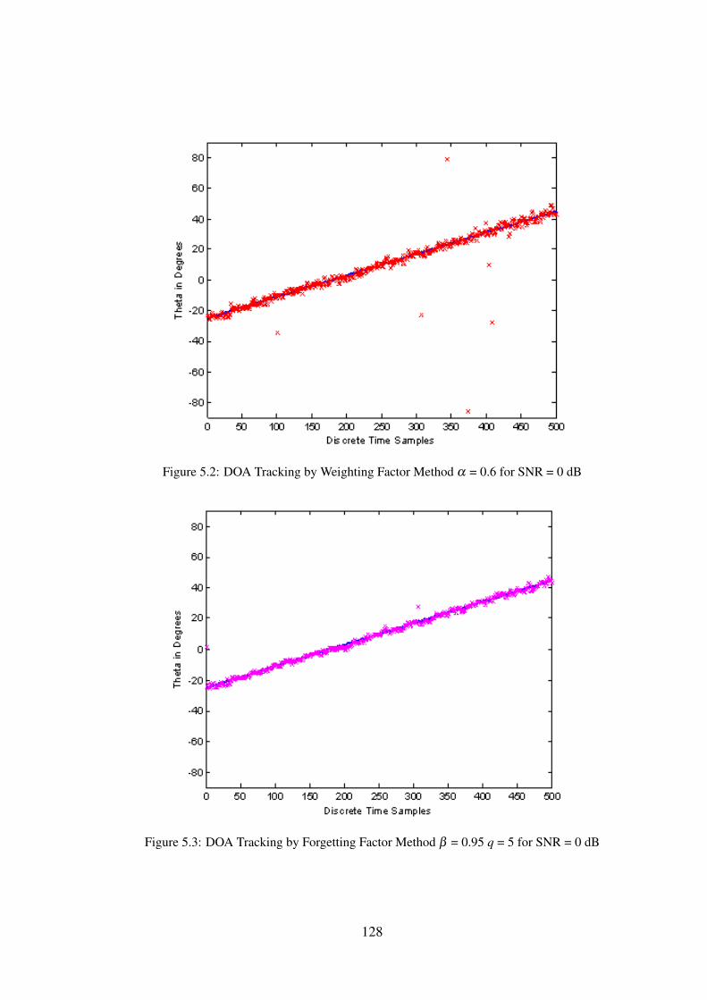
Figure 5.2: DOA Tracking by Weighting Factor Method α = 0.6 for SNR = 0 dB
Figure 5.3: DOA Tracking by Forgetting Factor Method β = 0.95 q = 5 for SNR = 0 dB
128
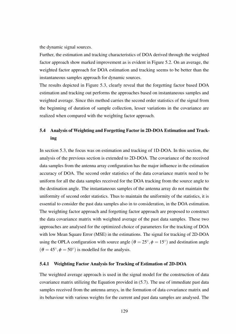
the dynamic signal sources.
Further, the estimation and tracking characteristics of DOA derived through the weighted
factor approach show marked improvement as is evident in Figure 5.2. On an average, the
weighted factor approach for DOA estimation and tracking seems to be better than the
instantaneous samples approach for dynamic sources.
The results depicted in Figure 5.3, clearly reveal that the forgetting factor based DOA
estimation and tracking out performs the approaches based on instantaneous samples and
weighted average. Since this method carries the second order statistics of the signal from
the beginning of duration of sample collection, lesser variations in the covariance are
realized when compared with the weighting factor approach.
5.4 Analysis of Weighting and Forgetting Factor in 2D-DOA Estimation and Track-ing
In section 5.3, the focus was on estimation and tracking of 1D-DOA. In this section, the
analysis of the previous section is extended to 2D-DOA. The covariance of the received
data samples from the antenna array configuration has the major influence in the estimation
accuracy of DOA. The second order statistics of the data covariance matrix need to be
uniform for all the data samples received for the DOA tracking from the source angle to
the destination angle. The instantaneous samples of the antenna array do not maintain the
uniformity of second order statistics. Thus to maintain the uniformity of the statistics, it is
essential to consider the past data samples also in to consideration, in the DOA estimation.
The weighting factor approach and forgetting factor approach are proposed to construct
the data covariance matrix with weighted average of the past data samples. These two
approaches are analysed for the optimized choice of parameters for the tracking of DOA
with low Mean Square Error (MSE) in the estimations. The signal for tracking of 2D-DOA
using the OPLA configuration with source angle (θ = 25◦,φ = 15◦) and destination angle
(θ = 45◦,φ = 50◦) is modelled for the analysis.
5.4.1 Weighting Factor Analysis for Tracking of Estimation of 2D-DOA
The weighted average approach is used in the signal model for the construction of data
covariance matrix utilizing the Equation provided in (5.7). The use of immediate past data
samples received from the antenna arrays, in the formation of data covariance matrix and
its behaviour with various weights for the current and past data samples are analysed. The
129
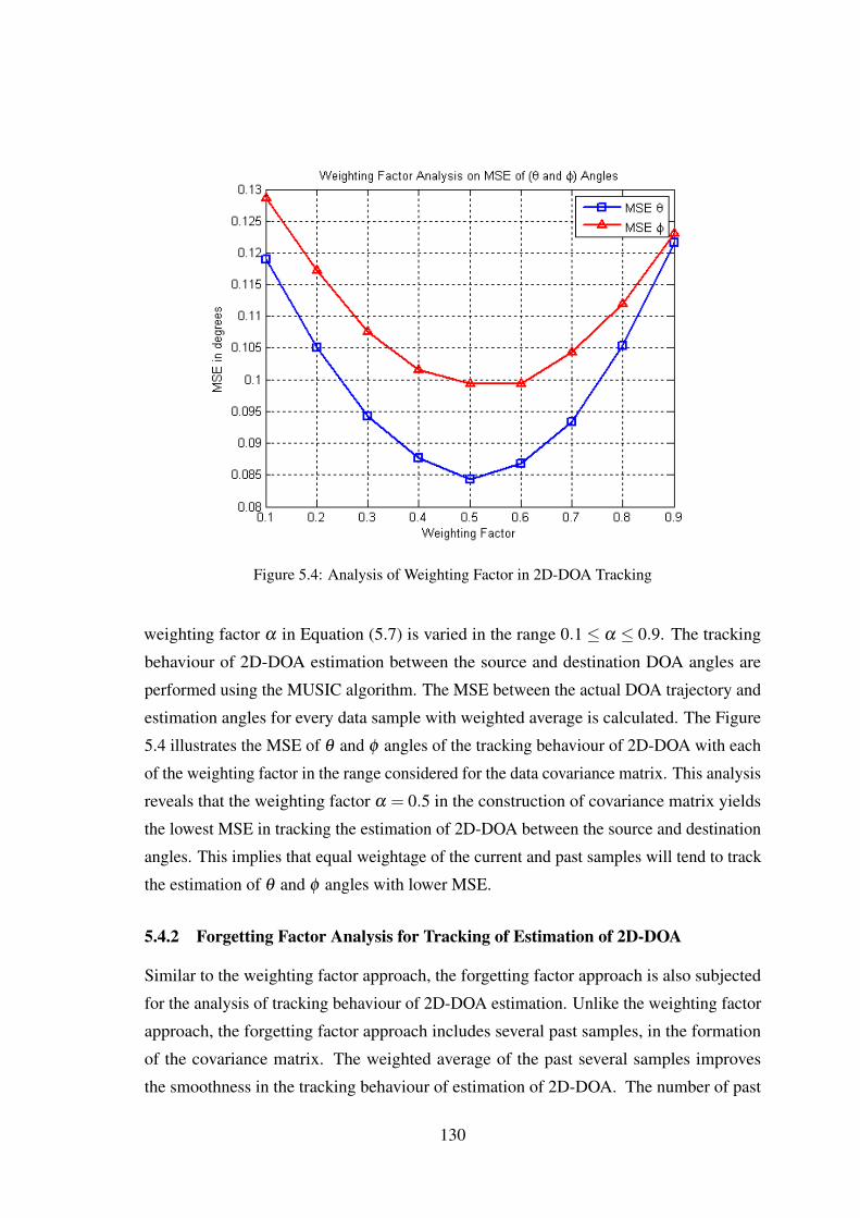
Figure 5.4: Analysis of Weighting Factor in 2D-DOA Tracking
weighting factor α in Equation (5.7) is varied in the range 0.1 ≤ α ≤ 0.9. The tracking
behaviour of 2D-DOA estimation between the source and destination DOA angles are
performed using the MUSIC algorithm. The MSE between the actual DOA trajectory and
estimation angles for every data sample with weighted average is calculated. The Figure
5.4 illustrates the MSE of θ and φ angles of the tracking behaviour of 2D-DOA with each
of the weighting factor in the range considered for the data covariance matrix. This analysis
reveals that the weighting factor α = 0.5 in the construction of covariance matrix yields
the lowest MSE in tracking the estimation of 2D-DOA between the source and destination
angles. This implies that equal weightage of the current and past samples will tend to track
the estimation of θ and φ angles with lower MSE.
5.4.2 Forgetting Factor Analysis for Tracking of Estimation of 2D-DOA
Similar to the weighting factor approach, the forgetting factor approach is also subjected
for the analysis of tracking behaviour of 2D-DOA estimation. Unlike the weighting factor
approach, the forgetting factor approach includes several past samples, in the formation
of the covariance matrix. The weighted average of the past several samples improves
the smoothness in the tracking behaviour of estimation of 2D-DOA. The number of past
130
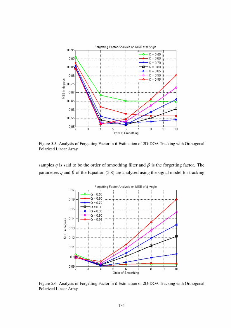
Figure 5.5: Analysis of Forgetting Factor in θ Estimation of 2D-DOA Tracking with OrthogonalPolarized Linear Array
samples q is said to be the order of smoothing filter and β is the forgetting factor. The
parameters q and β of the Equation (5.8) are analysed using the signal model for tracking
Figure 5.6: Analysis of Forgetting Factor in φ Estimation of 2D-DOA Tracking with OrthogonalPolarized Linear Array
131

behaviour of estimation of 2D-DOA for choosing the optimum choice of the filter order
and forgetting factor.
The order of the smoothing filter q is subjected for the analysis in the range 2≤ q≤ 10 in
steps of 2. The forgetting factor β in the range 0.5≤ β ≤ 0.95 with order of the filter is
analysed for the tracking behaviour of estimation of 2D-DOA. The results of the Figures 5.5
and 5.6 depict the MSE of θ and φ estimation respectively in 2D-DOA tracking behaviour
between the source and destination DOA angles. The results of the Figures 5.5 and 5.6
reveal that, in both θ and φ estimation error is very less at smoothing filter order of q =
4. This in turn conveys that only the immediate past 4 samples should be utilized for the
better estimation accuracy rather than considering the more number of past samples. The
combined analysis of the θ and φ estimation error, the forgetting factor β = 0.95 is more
suitable to be utilized for the lowest MSE with the filter order of q = 4, when compared
with the other forgetting factors in the range.
5.5 Analysis of 2D-DOA Tracking Behaviour of Single and Orthogonal PolarizedArrays
The two-dimensional DOA tracking behaviour is analysed for the conventional single
polarized and proposed orthogonal polarized array configurations. The following analyses
illustrate 2D-DOA tracking behaviour for the single and orthogonal polarized using the
instantaneous samples, weighting factor and forgetting factor approaches. The signal
model for the 2D-DOA tracking with source angle (θ = 25◦,φ = 15◦) and destination
angle (θ = 45◦,φ = 50◦) is modelled for the analysis with SNR of 20 dB. Between the
source and destination angles, 100 data samples are modelled for the trajectory. The 2D
MUSIC algorithm is used for the 2D tracking behaviour of the array configuration and
average error of the 2D-DOA estimation per data sample is computed through the MSE
performance analysis.
5.5.1 Tracking Behaviour of 2D-DOA Estimation with Single Polarized UPA
The conventional single polarized UPA configuration with rectangular waveguide shown
in Figure 4.1, is analysed for its performance in the 2D-DOA tracking behaviour for the
above mentioned signal model.
132
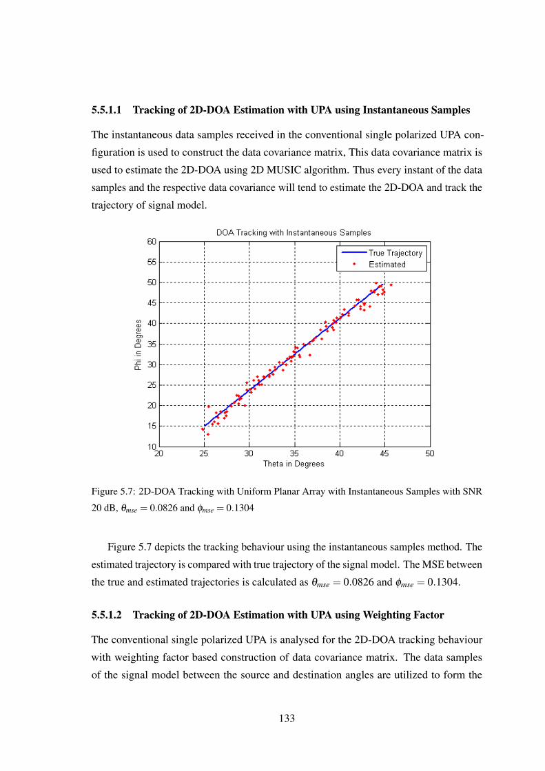
5.5.1.1 Tracking of 2D-DOA Estimation with UPA using Instantaneous Samples
The instantaneous data samples received in the conventional single polarized UPA con-
figuration is used to construct the data covariance matrix, This data covariance matrix is
used to estimate the 2D-DOA using 2D MUSIC algorithm. Thus every instant of the data
samples and the respective data covariance will tend to estimate the 2D-DOA and track the
trajectory of signal model.
Figure 5.7: 2D-DOA Tracking with Uniform Planar Array with Instantaneous Samples with SNR
20 dB, θmse = 0.0826 and φmse = 0.1304
Figure 5.7 depicts the tracking behaviour using the instantaneous samples method. The
estimated trajectory is compared with true trajectory of the signal model. The MSE between
the true and estimated trajectories is calculated as θmse = 0.0826 and φmse = 0.1304.
5.5.1.2 Tracking of 2D-DOA Estimation with UPA using Weighting Factor
The conventional single polarized UPA is analysed for the 2D-DOA tracking behaviour
with weighting factor based construction of data covariance matrix. The data samples
of the signal model between the source and destination angles are utilized to form the
133
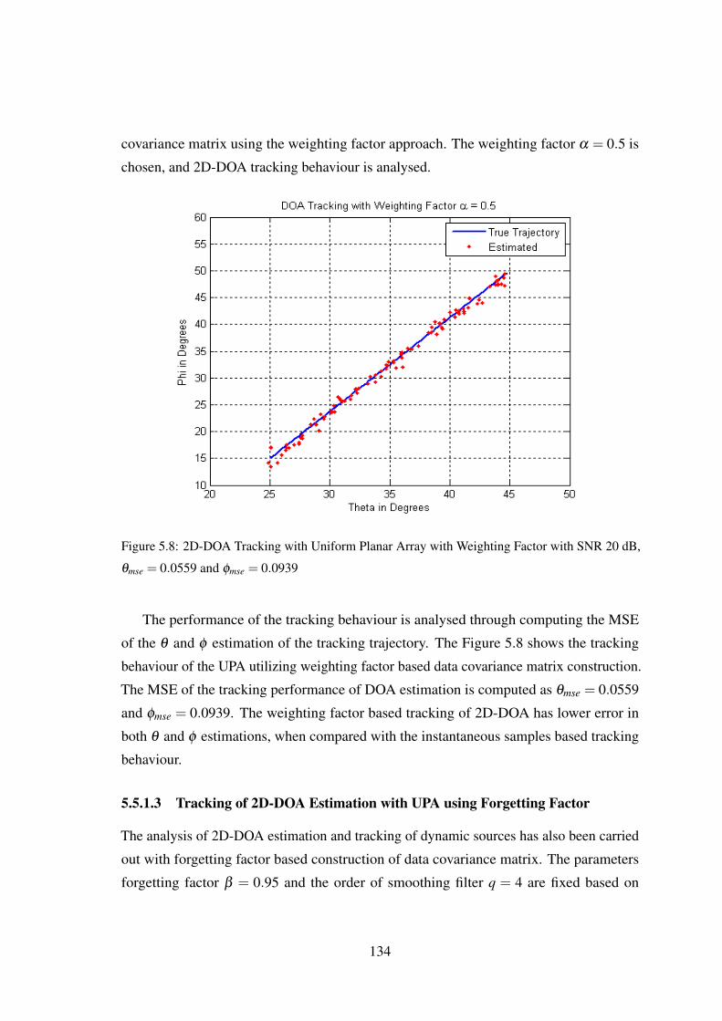
covariance matrix using the weighting factor approach. The weighting factor α = 0.5 is
chosen, and 2D-DOA tracking behaviour is analysed.
Figure 5.8: 2D-DOA Tracking with Uniform Planar Array with Weighting Factor with SNR 20 dB,
θmse = 0.0559 and φmse = 0.0939
The performance of the tracking behaviour is analysed through computing the MSE
of the θ and φ estimation of the tracking trajectory. The Figure 5.8 shows the tracking
behaviour of the UPA utilizing weighting factor based data covariance matrix construction.
The MSE of the tracking performance of DOA estimation is computed as θmse = 0.0559
and φmse = 0.0939. The weighting factor based tracking of 2D-DOA has lower error in
both θ and φ estimations, when compared with the instantaneous samples based tracking
behaviour.
5.5.1.3 Tracking of 2D-DOA Estimation with UPA using Forgetting Factor
The analysis of 2D-DOA estimation and tracking of dynamic sources has also been carried
out with forgetting factor based construction of data covariance matrix. The parameters
forgetting factor β = 0.95 and the order of smoothing filter q = 4 are fixed based on
134
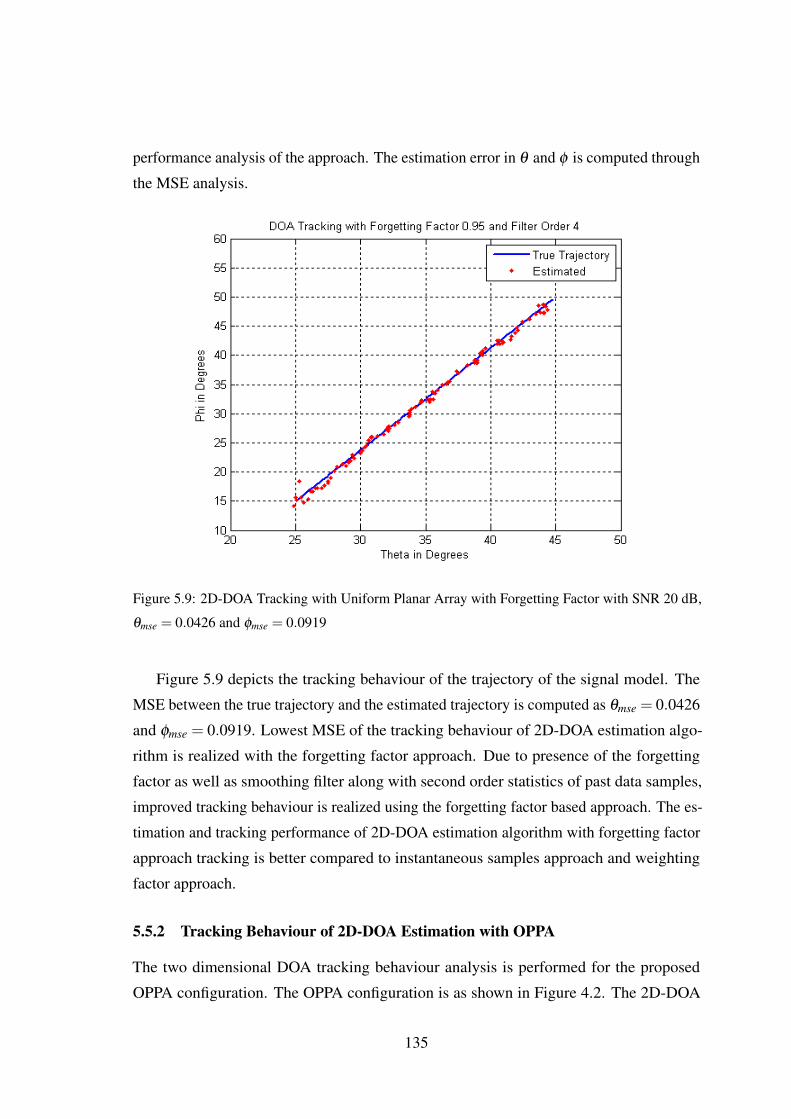
performance analysis of the approach. The estimation error in θ and φ is computed through
the MSE analysis.
Figure 5.9: 2D-DOA Tracking with Uniform Planar Array with Forgetting Factor with SNR 20 dB,
θmse = 0.0426 and φmse = 0.0919
Figure 5.9 depicts the tracking behaviour of the trajectory of the signal model. The
MSE between the true trajectory and the estimated trajectory is computed as θmse = 0.0426
and φmse = 0.0919. Lowest MSE of the tracking behaviour of 2D-DOA estimation algo-
rithm is realized with the forgetting factor approach. Due to presence of the forgetting
factor as well as smoothing filter along with second order statistics of past data samples,
improved tracking behaviour is realized using the forgetting factor based approach. The es-
timation and tracking performance of 2D-DOA estimation algorithm with forgetting factor
approach tracking is better compared to instantaneous samples approach and weighting
factor approach.
5.5.2 Tracking Behaviour of 2D-DOA Estimation with OPPA
The two dimensional DOA tracking behaviour analysis is performed for the proposed
OPPA configuration. The OPPA configuration is as shown in Figure 4.2. The 2D-DOA
135
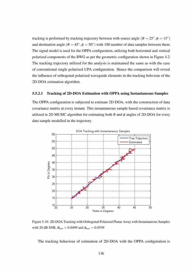
tracking is performed by tracking trajectory between with source angle (θ = 25◦,φ = 15◦)
and destination angle (θ = 45◦,φ = 50◦) with 100 number of data samples between them.
The signal model is used for the OPPA configuration, utilizing both horizontal and vertical
polarized components of the RWG as per the geometric configuration shown in Figure 4.2.
The tracking trajectory utilized for the analysis is maintained the same as with the case
of conventional single polarized UPA configuration. Hence the comparison will reveal
the influence of orthogonal polarized waveguide elements in the tracking behviour of the
2D-DOA estimation algorithm.
5.5.2.1 Tracking of 2D-DOA Estimation with OPPA using Instantaneous Samples
The OPPA configuration is subjected to estimate 2D-DOA, with the construction of data
covariance matrix at every instant. This instantaneous sample based covariance matrix is
utilized in 2D MUSIC algorithm for estimating both θ and φ angles of 2D-DOA for every
data sample modelled in the trajectory.
Figure 5.10: 2D-DOA Tracking with Orthogonal Polarized Planar Array with Instantaneous Samples
with 20 dB SNR, θmse = 0.0499 and φmse = 0.0559
The tracking behaviour of estimation of 2D-DOA with the OPPA configuration is
136
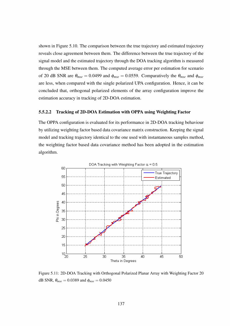
shown in Figure 5.10. The comparison between the true trajectory and estimated trajectory
reveals close agreement between them. The difference between the true trajectory of the
signal model and the estimated trajectory through the DOA tracking algorithm is measured
through the MSE between them. The computed average error per estimation for scenario
of 20 dB SNR are θmse = 0.0499 and φmse = 0.0559. Comparatively the θmse and φmse
are less, when compared with the single polarized UPA configuration. Hence, it can be
concluded that, orthogonal polarized elements of the array configuration improve the
estimation accuracy in tracking of 2D-DOA estimation.
5.5.2.2 Tracking of 2D-DOA Estimation with OPPA using Weighting Factor
The OPPA configuration is evaluated for its performance in 2D-DOA tracking behaviour
by utilizing weighting factor based data covariance matrix construction. Keeping the signal
model and tracking trajectory identical to the one used with instantaneous samples method,
the weighting factor based data covariance method has been adopted in the estimation
algorithm.
Figure 5.11: 2D-DOA Tracking with Orthogonal Polarized Planar Array with Weighting Factor 20
dB SNR, θmse = 0.0389 and φmse = 0.0450
137
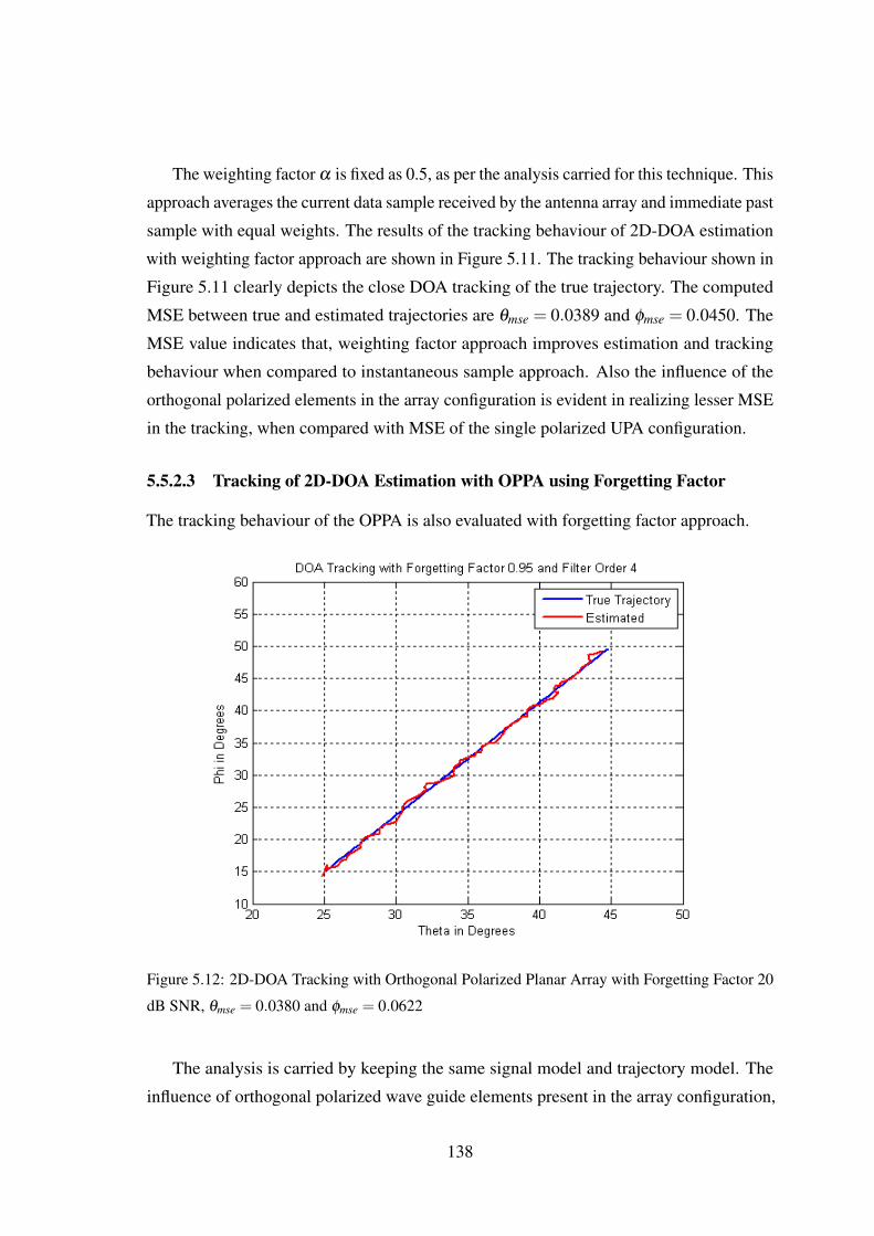
The weighting factor α is fixed as 0.5, as per the analysis carried for this technique. This
approach averages the current data sample received by the antenna array and immediate past
sample with equal weights. The results of the tracking behaviour of 2D-DOA estimation
with weighting factor approach are shown in Figure 5.11. The tracking behaviour shown in
Figure 5.11 clearly depicts the close DOA tracking of the true trajectory. The computed
MSE between true and estimated trajectories are θmse = 0.0389 and φmse = 0.0450. The
MSE value indicates that, weighting factor approach improves estimation and tracking
behaviour when compared to instantaneous sample approach. Also the influence of the
orthogonal polarized elements in the array configuration is evident in realizing lesser MSE
in the tracking, when compared with MSE of the single polarized UPA configuration.
5.5.2.3 Tracking of 2D-DOA Estimation with OPPA using Forgetting Factor
The tracking behaviour of the OPPA is also evaluated with forgetting factor approach.
Figure 5.12: 2D-DOA Tracking with Orthogonal Polarized Planar Array with Forgetting Factor 20
dB SNR, θmse = 0.0380 and φmse = 0.0622
The analysis is carried by keeping the same signal model and trajectory model. The
influence of orthogonal polarized wave guide elements present in the array configuration,
138

along with the forgetting factor based approach for the construction of covariance matrix
in improving the estimation accuracy is analysed. The parameters, forgetting factor and
order smoothing filter are fixed as β = 0.95 and q = 4 based on the detailed analysis
carried for this approach. The improved tracking behaviour of OPPA is depicted in the
Figure 5.12. It is seen from the results of the Figure 5.12, that there is a close agreement
of estimated trajectory of DOA with true trajectory and the same is evident through the
computation of MSE between them. The computed MSE between the estimated trajectory
and true trajectory are θmse = 0.0380 and φmse = 0.0622. The MSE value depicts the lesser
estimation error both in the θ and φ DOA angles, which has resulted in improved tracking
behaviour. The combination of forgetting factor approach and the orthogonal polarized
array elements is an effective combination in improving the estimation accuracy and the
tracking behaviour of 2D-DOA estimation algorithm.
5.5.3 Tracking Behaviour of 2D-DOA Estimation with OMLA
The simulation analysis of the tracking behaviour of 2D-DOA estimation is extended for
the OMLA configuration. In the OMLA, both the horizontal and vertical polarized waveg-
uide elements are combined together to form the orthogonal mounting. This orthogonal
mounting arrangement along the array axis as shown in Figure 4.3 is examined for its
performance in tracking of a 2D-DOA trajectory between the source and destination angles.
The signal model for the analysis is carried as per the geometric configuration of the array
elements and the trajectory modelled between the source angle (θ = 25◦,φ = 15◦) and
destination angle (θ = 45◦,φ = 50◦) with 100 number of data samples between them.
The OMLA configuration also has the orthogonal polarized (both horizontal and vertical)
elements. It is anticipated that, the estimation and tracking performance of 2D-DOA
estimation will be similar to that with the OPPA configuration.
5.5.3.1 Tracking of 2D-DOA Estimation with OMLA using Instantaneous Samples
The signal model and trajectory model for the OMLA are evaluated for 2D-DOA tracking
with the instantaneous sample method for the construction of data covariance matrix.
The data covariance matrix is subjected to 2D-DOA estimation algorithm and the MSE
performance of the 2D-DOA tracking is evaluated.
139
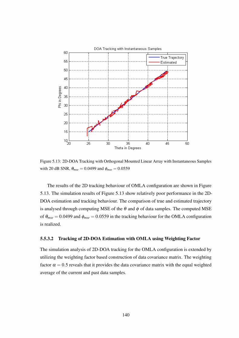
Figure 5.13: 2D-DOA Tracking with Orthogonal Mounted Linear Array with Instantaneous Samples
with 20 dB SNR, θmse = 0.0499 and φmse = 0.0559
The results of the 2D tracking behaviour of OMLA configuration are shown in Figure
5.13. The simulation results of Figure 5.13 show relatively poor performance in the 2D-
DOA estimation and tracking behaviour. The comparison of true and estimated trajectory
is analysed through computing MSE of the θ and φ of data samples. The computed MSE
of θmse = 0.0499 and φmse = 0.0559 in the tracking behaviour for the OMLA configuration
is realized.
5.5.3.2 Tracking of 2D-DOA Estimation with OMLA using Weighting Factor
The simulation analysis of 2D-DOA tracking for the OMLA configuration is extended by
utilizing the weighting factor based construction of data covariance matrix. The weighting
factor α = 0.5 reveals that it provides the data covariance matrix with the equal weighted
average of the current and past data samples.
140
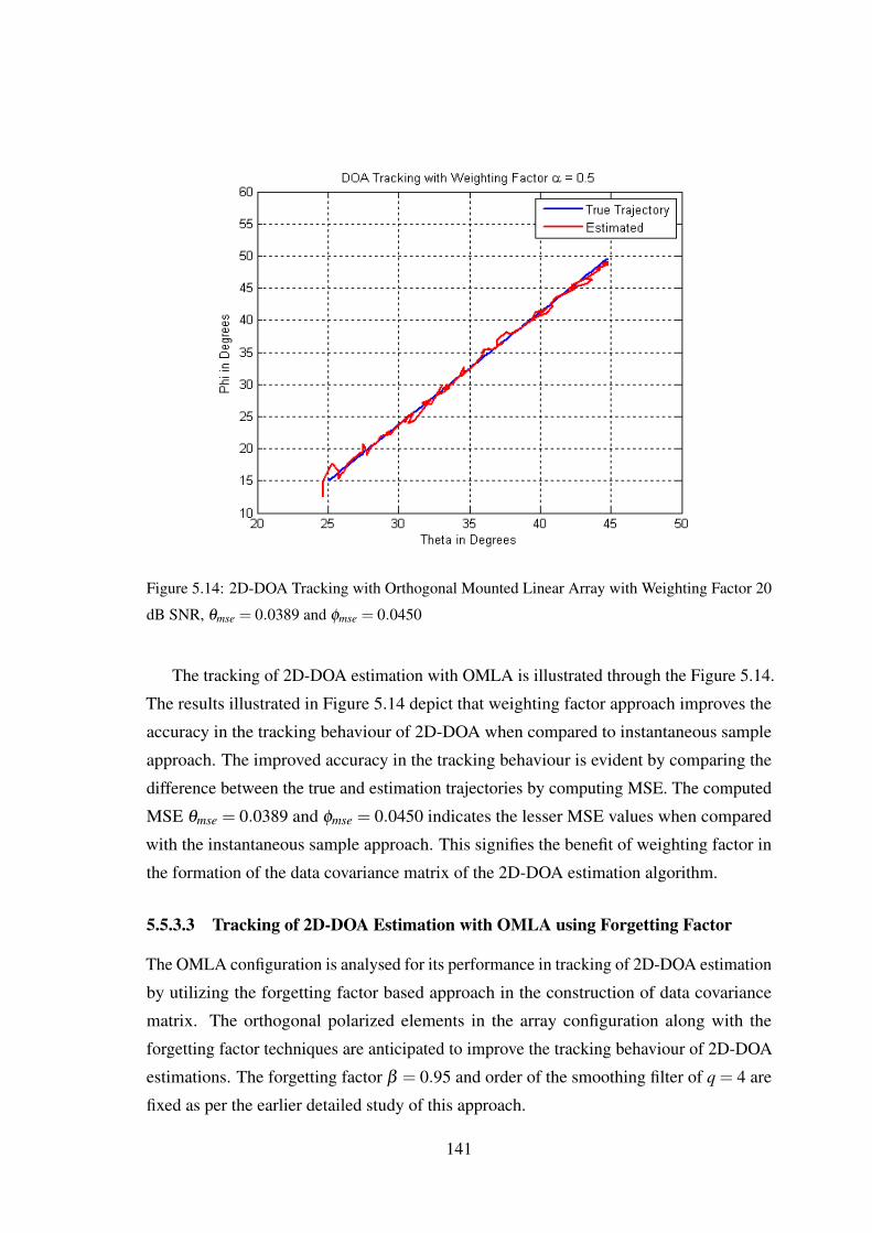
Figure 5.14: 2D-DOA Tracking with Orthogonal Mounted Linear Array with Weighting Factor 20
dB SNR, θmse = 0.0389 and φmse = 0.0450
The tracking of 2D-DOA estimation with OMLA is illustrated through the Figure 5.14.
The results illustrated in Figure 5.14 depict that weighting factor approach improves the
accuracy in the tracking behaviour of 2D-DOA when compared to instantaneous sample
approach. The improved accuracy in the tracking behaviour is evident by comparing the
difference between the true and estimation trajectories by computing MSE. The computed
MSE θmse = 0.0389 and φmse = 0.0450 indicates the lesser MSE values when compared
with the instantaneous sample approach. This signifies the benefit of weighting factor in
the formation of the data covariance matrix of the 2D-DOA estimation algorithm.
5.5.3.3 Tracking of 2D-DOA Estimation with OMLA using Forgetting Factor
The OMLA configuration is analysed for its performance in tracking of 2D-DOA estimation
by utilizing the forgetting factor based approach in the construction of data covariance
matrix. The orthogonal polarized elements in the array configuration along with the
forgetting factor techniques are anticipated to improve the tracking behaviour of 2D-DOA
estimations. The forgetting factor β = 0.95 and order of the smoothing filter of q = 4 are
fixed as per the earlier detailed study of this approach.
141
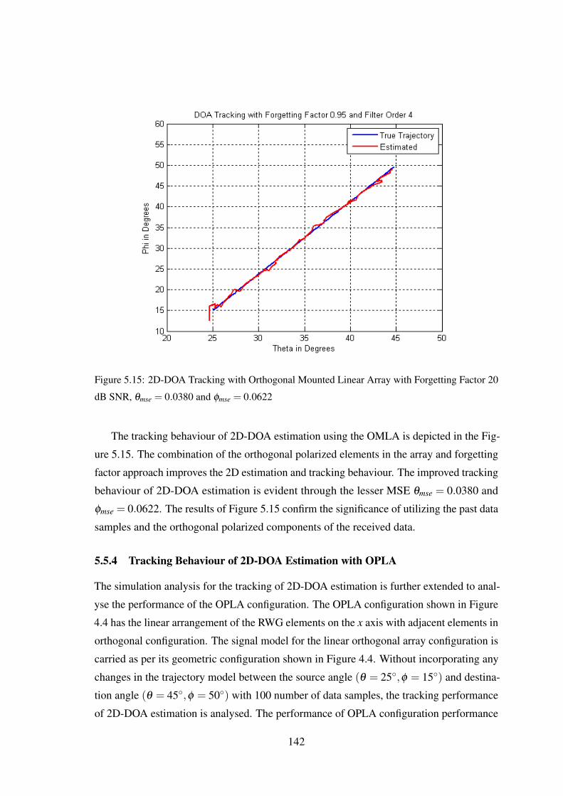
Figure 5.15: 2D-DOA Tracking with Orthogonal Mounted Linear Array with Forgetting Factor 20
dB SNR, θmse = 0.0380 and φmse = 0.0622
The tracking behaviour of 2D-DOA estimation using the OMLA is depicted in the Fig-
ure 5.15. The combination of the orthogonal polarized elements in the array and forgetting
factor approach improves the 2D estimation and tracking behaviour. The improved tracking
behaviour of 2D-DOA estimation is evident through the lesser MSE θmse = 0.0380 and
φmse = 0.0622. The results of Figure 5.15 confirm the significance of utilizing the past data
samples and the orthogonal polarized components of the received data.
5.5.4 Tracking Behaviour of 2D-DOA Estimation with OPLA
The simulation analysis for the tracking of 2D-DOA estimation is further extended to anal-
yse the performance of the OPLA configuration. The OPLA configuration shown in Figure
4.4 has the linear arrangement of the RWG elements on the x axis with adjacent elements in
orthogonal configuration. The signal model for the linear orthogonal array configuration is
carried as per its geometric configuration shown in Figure 4.4. Without incorporating any
changes in the trajectory model between the source angle (θ = 25◦,φ = 15◦) and destina-
tion angle (θ = 45◦,φ = 50◦) with 100 number of data samples, the tracking performance
of 2D-DOA estimation is analysed. The performance of OPLA configuration performance
142

in tracking of 2D-DOA estimation is evaluated through computing the MSE between the
true and estimated trajectories.
5.5.4.1 Tracking of 2D-DOA Estimation with OPLA using Instantaneous Samples
The signal model and the trajectory model are subjected to the tracking analysis of 2D-
DOA estimation by utilizing the instantaneous samples of the model, for the formation of
data covariance matrix. This data covariance matrix is incorporated into the 2D MUSIC
algorithm, through which 2D-DOA estimation is performed.
Figure 5.16: 2D-DOA Tracking with Orthogonal Polarized Linear Array with Instantaneous Samples
with 20 dB SNR, θmse = 0.1386 and φmse = 0.1351
The OPLA exhibits its tracking behaviour of 2D-DOA estimation as shown in Figure
5.16. The comparison between the true trajectory and the estimated trajectory is computed
is analysed through MSE between them, and the computed MSE is θmse = 0.1386 and
φmse = 0.1351. The MSE of the 2D-DOA tracking with OPLA is slightly higher, when
compared with the other array configurations presented earlier. Slightly higher MSE is
attributed to the only linear arrangement of the array elements despite the presence of
orthogonal elements.
143
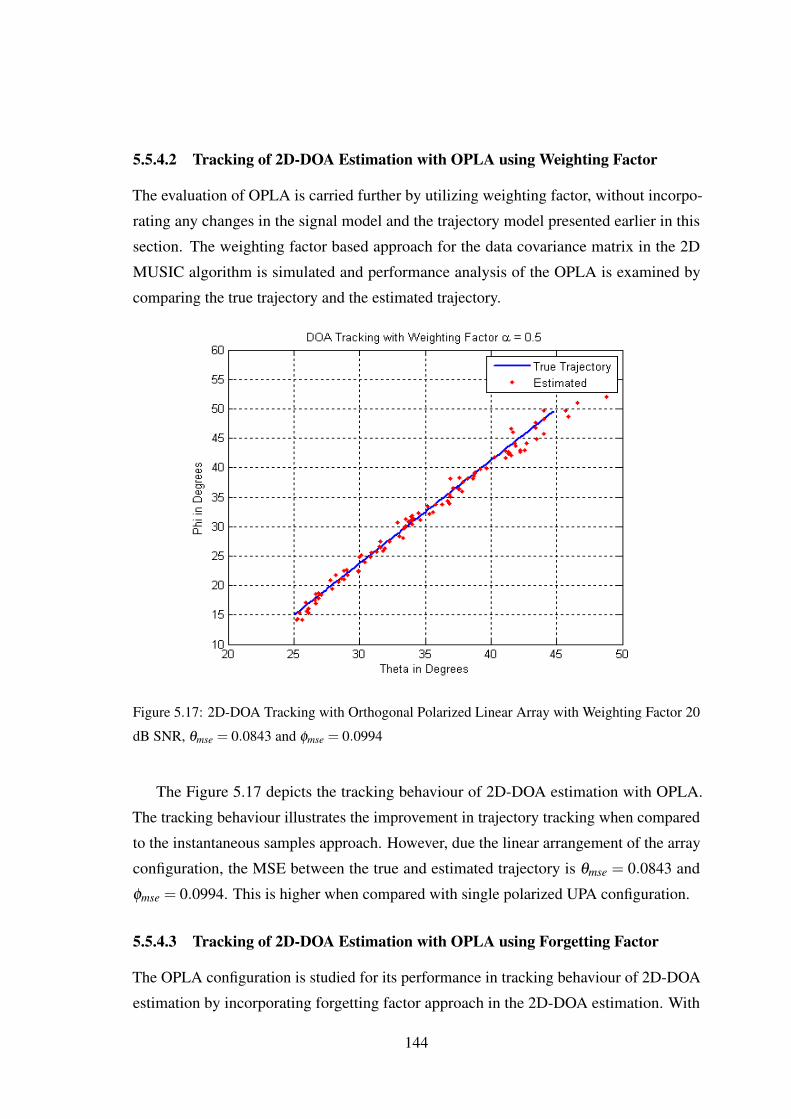
5.5.4.2 Tracking of 2D-DOA Estimation with OPLA using Weighting Factor
The evaluation of OPLA is carried further by utilizing weighting factor, without incorpo-
rating any changes in the signal model and the trajectory model presented earlier in this
section. The weighting factor based approach for the data covariance matrix in the 2D
MUSIC algorithm is simulated and performance analysis of the OPLA is examined by
comparing the true trajectory and the estimated trajectory.
Figure 5.17: 2D-DOA Tracking with Orthogonal Polarized Linear Array with Weighting Factor 20
dB SNR, θmse = 0.0843 and φmse = 0.0994
The Figure 5.17 depicts the tracking behaviour of 2D-DOA estimation with OPLA.
The tracking behaviour illustrates the improvement in trajectory tracking when compared
to the instantaneous samples approach. However, due the linear arrangement of the array
configuration, the MSE between the true and estimated trajectory is θmse = 0.0843 and
φmse = 0.0994. This is higher when compared with single polarized UPA configuration.
5.5.4.3 Tracking of 2D-DOA Estimation with OPLA using Forgetting Factor
The OPLA configuration is studied for its performance in tracking behaviour of 2D-DOA
estimation by incorporating forgetting factor approach in the 2D-DOA estimation. With
144

no modifications in the signal and trajectory model, simulation of OPLA with forgetting
factor approach of covariance data matrix is performed and the performance is analysed
through the MSE between the true and estimated trajectories.
Figure 5.18: 2D-DOA Tracking with Orthogonal Polarized Linear Array with Forgetting Factor 20
dB SNR, θmse = 0.0515 and φmse = 0.0952
The results of the tracking of 2D-DOA estimation with OPLA are shown in Figure 5.18.
The results of Figure 5.18 illustrate close agreement in tracking behaviour, by estimating
the 2D-DOA to be very close to the actual DOAs. The improvement in the tracking
behaviour of 2D-DOA estimation using forgetting factor approach is evident through lesser
MSE between the estimation and true trajectories, which is computed as θmse = 0.0515
and φmse = 0.0952.
5.6 Computation Analysis of MSE versus SNR in Tracking Behaviour of 2D-DOAEstimation with Single Polarized and Orthogonal Polarized Arrays
In the previous section, the analysis of the tracking behaviour of 2D-DOA estimation
is evaluated for single and orthogonal polarized array configurations with 20 dB SNR.
The simulation analysis is extended further to analyse the tracking behaviour of 2D-DOA
145
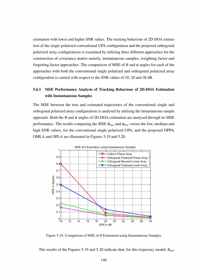
estimation with lower and higher SNR values. The tracking behaviour of 2D-DOA estima-
tion of the single polarized conventional UPA configuration and the proposed orthogonal
polarized array configurations is examined by utilizing three different approaches for the
construction of covariance matrix namely, instantaneous samples, weighting factor and
forgetting factor approaches. The comparison of MSE of θ and φ angles for each of the
approaches with both the conventional single polarized and orthogonal polarized array
configuration is carried with respect to the SNR values of 10, 20 and 30 dB.
5.6.1 MSE Performance Analysis of Tracking Behaviour of 2D-DOA Estimationwith Instantaneous Samples
The MSE between the true and estimated trajectories of the conventional single and
orthogonal polarized array configurations is analysed by utilizing the instantaneous sample
approach. Both the θ and φ angles of 2D-DOA estimation are analysed through its MSE
performance. The results comparing the MSE θmse and φmse versus the low, medium and
high SNR values, for the conventional single polarized UPA, and the proposed OPPA,
OMLA and OPLA are illustrated in Figures 5.19 and 5.20.
Figure 5.19: Comparison of MSE of θ Estimation using Instantaneous Samples
The results of the Figures 5.19 and 5.20 indicate that, for this trajectory model, θmse
146
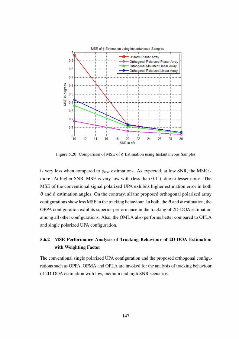
Figure 5.20: Comparison of MSE of φ Estimation using Instantaneous Samples
is very less when compared to φmse estimations. As expected, at low SNR, the MSE is
more. At higher SNR, MSE is very low with (less than 0.1◦), due to lesser noise. The
MSE of the conventional signal polarized UPA exhibits higher estimation error in both
θ and φ estimation angles. On the contrary, all the proposed orthogonal polarized array
configurations show less MSE in the tracking behaviour. In both, the θ and φ estimation, the
OPPA configuration exhibits superior performance in the tracking of 2D-DOA estimation
among all other configurations. Also, the OMLA also performs better compared to OPLA
and single polarized UPA configuration.
5.6.2 MSE Performance Analysis of Tracking Behaviour of 2D-DOA Estimationwith Weighting Factor
The conventional single polarized UPA configuration and the proposed orthogonal configu-
rations such as OPPA, OPMA and OPLA are invoked for the analysis of tracking behaviour
of 2D-DOA estimation with low, medium and high SNR scenarios.
147

Figure 5.21: Comparison of MSE of θ Estimation using Weighting Factor
Figure 5.22: Comparison of MSE of φ Estimation using Weighting Factor
148
The analysis is carried by incorporating weighting factor approach for data covariance
matrix in the 2D-DOA estimation and tracking. A weighting factor α = 0.5 is incorporated
in the construction of data covariance matrix, which induces the weighted average of the
current and immediate past data samples. The simulation analysis with weighting factor
approach is illustrated by plots of MSE versus SNR for the conventional single polarized
array configuration and the proposed orthogonal polarized array configurations. The MSE
θmse and φmse for all the array configurations are shown in Figures 5.21 and 5.22 respectively.
The results of the Figures 5.21 and 5.22 clearly depict the performance improvement in the
tracking behaviour of 2D-DOA estimation of all the array configuration, when compared
to instantaneous samples approach. The consistency in the improved tracking behaviour
of 2D-DOA estimation is evident in both the θmse and φmse of estimations for all the array
configurations. At low SNRs, all the array configurations exhibit lesser than 0.4◦ estimation
error in both the θ and φ estimations. The analysis invariably infers that, OPPA is best
among all other array configurations, in the tracking behaviour of the trajectory of 2D-DOA,
by estimating θ and φ with least MSE values. The OMLA configuration continues to
perform better, when compared to OPLA and single polarized UPA configurations. The
OPLA shows a slightly inferior performance in its θ estimations at lower SNR, when
compared to the single polarized UPA configuration. The φ angle estimations with OPLA
is more accurate when compared to single polarized UPA configuration. However, at
medium and higher SNR scenarios, the OPLA and UPA show on an average the same
tracking behaviour with negligibly small difference.
5.6.3 MSE Performance Analysis of Tracking Behaviour of 2D-DOA Estimationwith Forgetting Factor
The MSE performance analysis for the low, medium and high SNR scenarios is extended
further with formation of data covariance matrix with forgetting factor approach. The
conventional single polarized UPA as well as the proposed OPPA, OMLA and OPLA
configuration are analysed for its MSE performance by incorporating the forgetting factor
approach in the formation of data covariance matrix in the 2D-DOA estimation and tracking
technique.
149
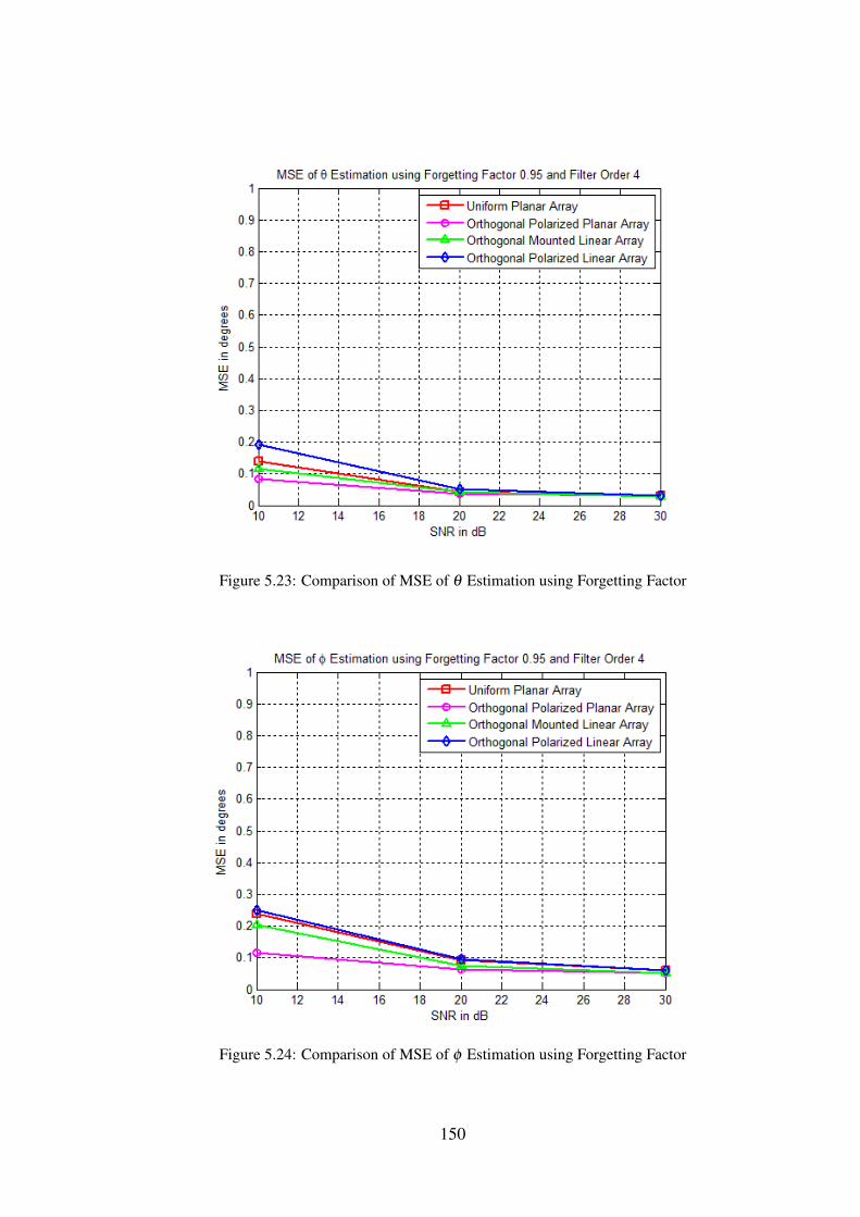
Figure 5.23: Comparison of MSE of θ Estimation using Forgetting Factor
Figure 5.24: Comparison of MSE of φ Estimation using Forgetting Factor
150

The forgetting factor β = 0.95 and order of the smoothing filter q = 4 are incorporated
in the simulation based on the extensive analysis of the approach. The tracking behaviour
of 2D-DOA estimation with forgetting factor approach is superior in its performance, which
is evident from the previous analysis presented earlier. The tracking behaviour of 2D-DOA
estimation realized with forgetting factor based covariance matrix is consistently better
when compared to those realized with the instantaneous approach as well as weighting
factor approach. The results of the Figures 5.23 and 5.24 exhibiting the better MSE
performance of θ and φ respectively are clear indicators of the superior performance of
2D-DOA tracking behaviour. The forgetting factor approach shows the MSE lesser than
0.25◦ at lower SNR scenario, which is the least estimation error, when compared to the
instantaneous and weighting factor approaches. The results of the Figures 5.23 and 5.24
infer the individual performance of the array configurations considered in the simulation
analysis. The OPPA configuration continues to exhibit least estimation error in both, θ and
φ estimations, and thus shows the superior performance in the trajectory estimation of 2D-
DOA. The OMLA proves to be next best alternate to OPPA configuration in the estimation
accuracy of both θ and φ angles. The OPLA and the UPA configurations show similar
performance as with case of weighting factor approach with reduced estimation error. The
linear arrangement of elements in OPLA for 2D-DOA estimation limits the estimation
performance at low SNR, when compared with the single polarized UPA configuration.
However, the advantage of linear arrangement can also be factor that needs to be considered
along the estimation accuracy.
151
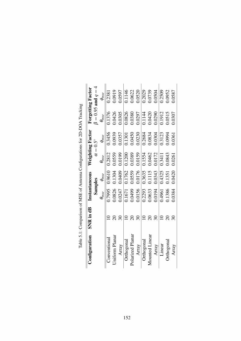
Tabl
e5.
1:C
ompa
riso
nof
MSE
ofA
nten
naC
onfig
urat
ions
for2
D-D
OA
Trac
king
Con
figur
atio
nSN
Rin
dBIn
stan
tane
ous
Wei
ghtin
gFa
ctor
Forg
ettin
gFa
ctor
Sam
ples
α=
0.5◦
β=
0.95
and
q=
4θ
mse
φm
seθ
mse
φm
seθ
mse
φm
se
Con
vent
iona
l10
0.79
950.
9610
0.28
120.
3456
0.13
760.
2381
Uni
form
Plan
ar20
0.08
260.
1304
0.05
590.
0939
0.04
260.
0919
Arr
ay30
0.02
470.
0409
0.01
990.
0357
0.03
050.
0597
Ort
hogo
nal
100.
1671
0.17
620.
1200
0.13
010.
0826
0.11
46Po
lari
zed
Plan
ar20
0.04
990.
0559
0.03
890.
0450
0.03
800.
0622
Arr
ay30
0.01
560.
0176
0.01
590.
0230
0.02
970.
0520
Ort
hogo
nal
100.
2293
0.36
350.
1554
0.26
840.
1144
0.20
29M
ount
edL
inea
r20
0.06
330.
1115
0.04
620.
0834
0.04
200.
0739
Arr
ay30
0.01
940.
0343
0.01
720.
0304
0.02
900.
0504
Lin
ear
100.
4961
0.43
250.
3411
0.31
230.
1912
0.25
09O
rtho
gona
l20
0.13
860.
1351
0.08
430.
0994
0.05
150.
0952
Arr
ay30
0.03
840.
0420
0.02
610.
0361
0.03
070.
0587
152
5.7 Summary
The simulation analysis of 2D-DOA estimation and tracking using the conventional sin-
gle polarized and orthogonal polarized array configurations are performed. The tracking
behaviour of 2D-DOA estimation with various array configurations are analysed by compar-
ing the computed MSE between true trajectory of the signal model and estimated trajectory.
Different schemes such as instantaneous samples approach, weighting factor approach and
forgetting factor approach have been utilized for the formation of data covariance matrix
involved in the MUSIC algorithm. The resulting MSEs for θ and φ angles of 2D-DOA are
computed using the data covariance matrix using three different approaches. The results of
the various analysis are tabulated for the low, medium and high SNR scenarios in the Table
5.1.
153

Chapter 6
DOA Estimation of Wideband Sources
This chapter presents the analysis and simulation of 1D and 2D-DOA estimation of
wideband signal sources. A comparison of performance between the conventional wideband
DOA estimation schemes with proposed subband filter approach is carried. A study on
proposed subband filter approach for 2D-DOA estimation of wideband sources with single
polarized UPA and the orthogonal polarized array configurations is performed for single
and two sources for a wide range of SNR scenarios.
6.1 Introduction
Further to the analysis of 2D-DOA estimation and tracking, the single polarised conven-
tional UPA and the proposed orthogonal polarized array configurations are evaluated for
the 2D-DOA estimation of wideband signal sources. A signal whose energy is spread
over a bandwidth, that is large in comparison to the signal center frequency is said to be
wideband signal. The estimation of the DOA of wave-fronts carrying wideband signal
is one of the critical tasks in DOA estimation. The rotational signal subspace and signal
subspace transformation and many beamspace processing techniques are cited in literature
for DOA of wideband sources (Sellone, 2005). The localization of a wideband signal
exploiting the array of wideband antenna elements using the conventional narrow band
techniques will fail. The limitation of narrowband techniques is that they exploit only the
time delays which directly translate to a phase shift in the frequency domain (Stoica &
Moses, 1997; Yoon, 2004). The performance of the subband filter approach for wideband
2D-DOA estimation, proposed in this chapter has been compared with performance of
conventional ICM and CSSM techniques discussed in Chapter 2.
Conventionally DOA estimation is carried through CSSM and ICM methods. In CSSM,
averaging of the spectrum is carried out after the focusing (transformation) of the subspace
vectors to the desired frequency. Whereas in ICM, the averaging is performed without
the transformation of subspace vectors. However the number of subspace computations
154
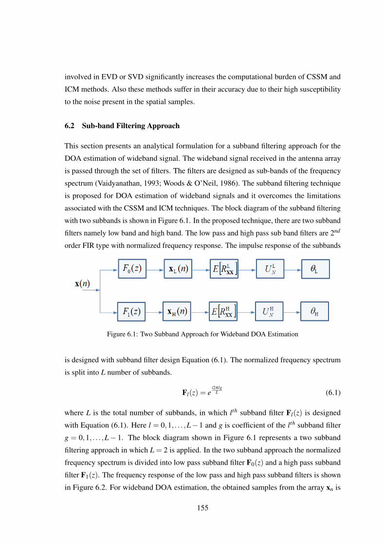
involved in EVD or SVD significantly increases the computational burden of CSSM and
ICM methods. Also these methods suffer in their accuracy due to their high susceptibility
to the noise present in the spatial samples.
6.2 Sub-band Filtering Approach
This section presents an analytical formulation for a subband filtering approach for the
DOA estimation of wideband signal. The wideband signal received in the antenna array
is passed through the set of filters. The filters are designed as sub-bands of the frequency
spectrum (Vaidyanathan, 1993; Woods & O’Neil, 1986). The subband filtering technique
is proposed for DOA estimation of wideband signals and it overcomes the limitations
associated with the CSSM and ICM techniques. The block diagram of the subband filtering
with two subbands is shown in Figure 6.1. In the proposed technique, there are two subband
filters namely low band and high band. The low pass and high pass sub band filters are 2nd
order FIR type with normalized frequency response. The impulse response of the subbands
Figure 6.1: Two Subband Approach for Wideband DOA Estimation
is designed with subband filter design Equation (6.1). The normalized frequency spectrum
is split into L number of subbands.
Fl(z) = ei2πlg
L (6.1)
where L is the total number of subbands, in which lth subband filter Fl(z) is designed
with Equation (6.1). Here l = 0,1, . . . ,L−1 and g is coefficient of the lth subband filter
g = 0,1, . . . ,L− 1. The block diagram shown in Figure 6.1 represents a two subband
filtering approach in which L = 2 is applied. In the two subband approach the normalized
frequency spectrum is divided into low pass subband filter F0(z) and a high pass subband
filter F1(z). The frequency response of the low pass and high pass subband filters is shown
in Figure 6.2. For wideband DOA estimation, the obtained samples from the array xn is
155
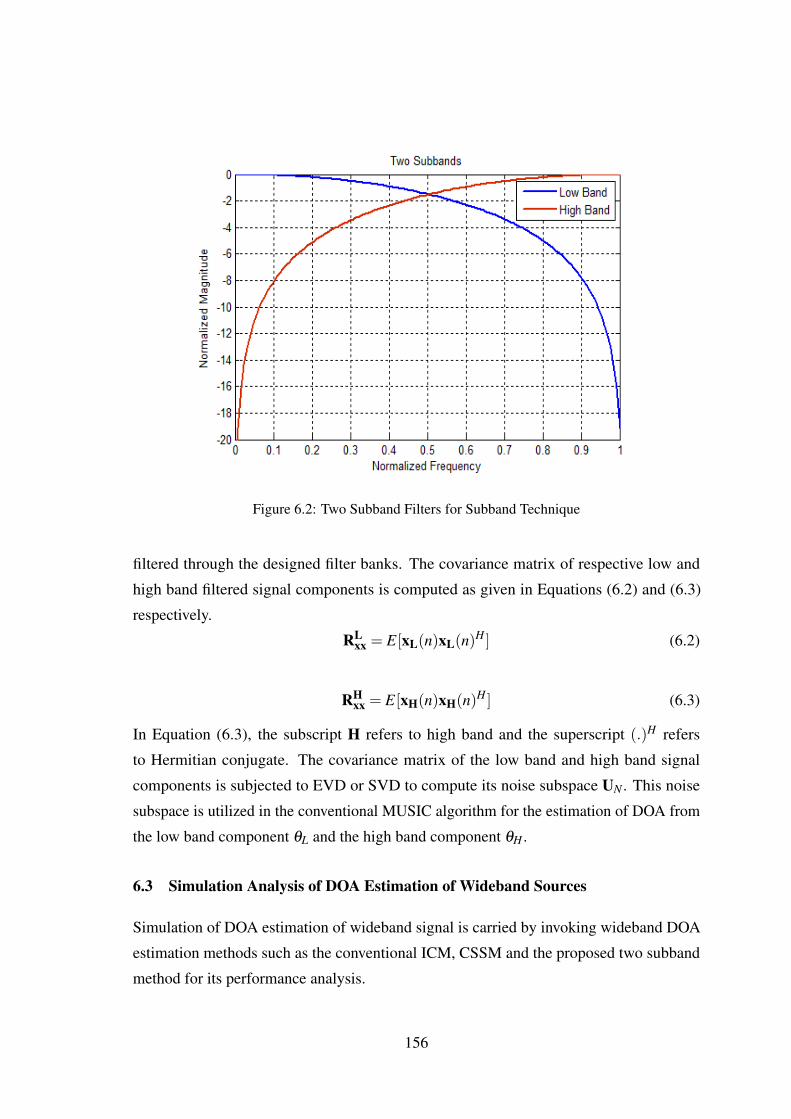
Figure 6.2: Two Subband Filters for Subband Technique
filtered through the designed filter banks. The covariance matrix of respective low and
high band filtered signal components is computed as given in Equations (6.2) and (6.3)
respectively.
RLxx = E[xL(n)xL(n)H ] (6.2)
RHxx = E[xH(n)xH(n)H ] (6.3)
In Equation (6.3), the subscript H refers to high band and the superscript (.)H refers
to Hermitian conjugate. The covariance matrix of the low band and high band signal
components is subjected to EVD or SVD to compute its noise subspace UN . This noise
subspace is utilized in the conventional MUSIC algorithm for the estimation of DOA from
the low band component θL and the high band component θH .
6.3 Simulation Analysis of DOA Estimation of Wideband Sources
Simulation of DOA estimation of wideband signal is carried by invoking wideband DOA
estimation methods such as the conventional ICM, CSSM and the proposed two subband
method for its performance analysis.
156
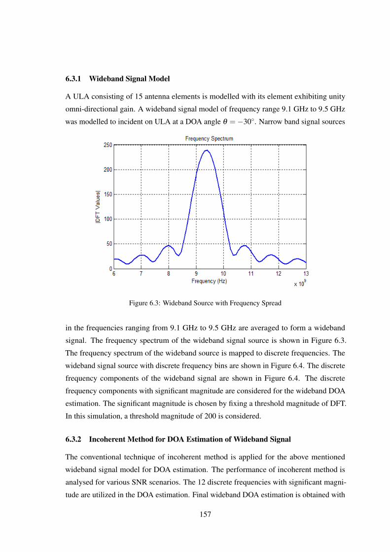
6.3.1 Wideband Signal Model
A ULA consisting of 15 antenna elements is modelled with its element exhibiting unity
omni-directional gain. A wideband signal model of frequency range 9.1 GHz to 9.5 GHz
was modelled to incident on ULA at a DOA angle θ =−30◦. Narrow band signal sources
Figure 6.3: Wideband Source with Frequency Spread
in the frequencies ranging from 9.1 GHz to 9.5 GHz are averaged to form a wideband
signal. The frequency spectrum of the wideband signal source is shown in Figure 6.3.
The frequency spectrum of the wideband source is mapped to discrete frequencies. The
wideband signal source with discrete frequency bins are shown in Figure 6.4. The discrete
frequency components of the wideband signal are shown in Figure 6.4. The discrete
frequency components with significant magnitude are considered for the wideband DOA
estimation. The significant magnitude is chosen by fixing a threshold magnitude of DFT.
In this simulation, a threshold magnitude of 200 is considered.
6.3.2 Incoherent Method for DOA Estimation of Wideband Signal
The conventional technique of incoherent method is applied for the above mentioned
wideband signal model for DOA estimation. The performance of incoherent method is
analysed for various SNR scenarios. The 12 discrete frequencies with significant magni-
tude are utilized in the DOA estimation. Final wideband DOA estimation is obtained with
157

Figure 6.4: Wideband Source Mapped to Discrete Frequencies
the product of the each estimation with discrete frequencies. Each of discrete frequency
components of wideband signal spectrum and its DOA estimation for 30 dB SNR are
shown in Figure 6.5. Figure 6.5 shows individual discrete frequencies of wideband source
Figure 6.5: Wideband DOA Estimation with Discrete Frequencies of Incoherent Method with 30dB SNR
158
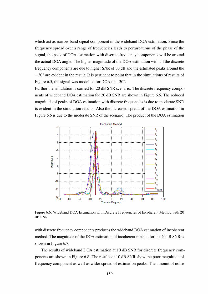
which act as narrow band signal component in the wideband DOA estimation. Since the
frequency spread over a range of frequencies leads to perturbations of the phase of the
signal, the peak of DOA estimation with discrete frequency components will be around
the actual DOA angle. The higher magnitude of the DOA estimation with all the discrete
frequency components are due to higher SNR of 30 dB and the estimated peaks around the
−30◦ are evident in the result. It is pertinent to point that in the simulations of results of
Figure 6.5, the signal was modelled for DOA of −30◦.
Further the simulation is carried for 20 dB SNR scenario. The discrete frequency compo-
nents of wideband DOA estimation for 20 dB SNR are shown in Figure 6.6. The reduced
magnitude of peaks of DOA estimation with discrete frequencies is due to moderate SNR
is evident in the simulation results. Also the increased spread of the DOA estimation in
Figure 6.6 is due to the moderate SNR of the scenario. The product of the DOA estimation
Figure 6.6: Wideband DOA Estimation with Discrete Frequencies of Incoherent Method with 20dB SNR
with discrete frequency components produces the wideband DOA estimation of incoherent
method. The magnitude of the DOA estimation of incoherent method for the 20 dB SNR is
shown in Figure 6.7.
The results of wideband DOA estimation at 10 dB SNR for discrete frequency com-
ponents are shown in Figure 6.8. The results of 10 dB SNR show the poor magnitude of
frequency component as well as wider spread of estimation peaks. The amount of noise
159
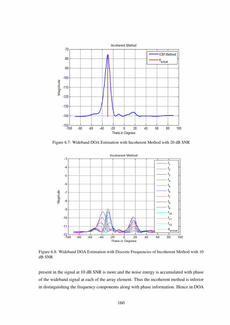
Figure 6.7: Wideband DOA Estimation with Incoherent Method with 20 dB SNR
Figure 6.8: Wideband DOA Estimation with Discrete Frequencies of Incoherent Method with 10dB SNR
present in the signal at 10 dB SNR is more and the noise energy is accumulated with phase
of the wideband signal at each of the array element. Thus the incoherent method is inferior
in distinguishing the frequency components along with phase information. Hence in DOA
160
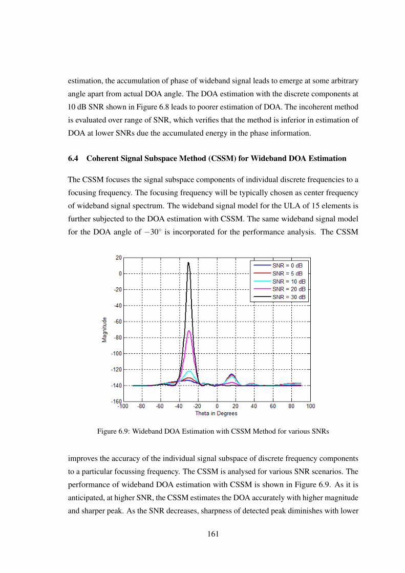
estimation, the accumulation of phase of wideband signal leads to emerge at some arbitrary
angle apart from actual DOA angle. The DOA estimation with the discrete components at
10 dB SNR shown in Figure 6.8 leads to poorer estimation of DOA. The incoherent method
is evaluated over range of SNR, which verifies that the method is inferior in estimation of
DOA at lower SNRs due the accumulated energy in the phase information.
6.4 Coherent Signal Subspace Method (CSSM) for Wideband DOA Estimation
The CSSM focuses the signal subspace components of individual discrete frequencies to a
focusing frequency. The focusing frequency will be typically chosen as center frequency
of wideband signal spectrum. The wideband signal model for the ULA of 15 elements is
further subjected to the DOA estimation with CSSM. The same wideband signal model
for the DOA angle of −30◦ is incorporated for the performance analysis. The CSSM
Figure 6.9: Wideband DOA Estimation with CSSM Method for various SNRs
improves the accuracy of the individual signal subspace of discrete frequency components
to a particular focussing frequency. The CSSM is analysed for various SNR scenarios. The
performance of wideband DOA estimation with CSSM is shown in Figure 6.9. As it is
anticipated, at higher SNR, the CSSM estimates the DOA accurately with higher magnitude
and sharper peak. As the SNR decreases, sharpness of detected peak diminishes with lower
161
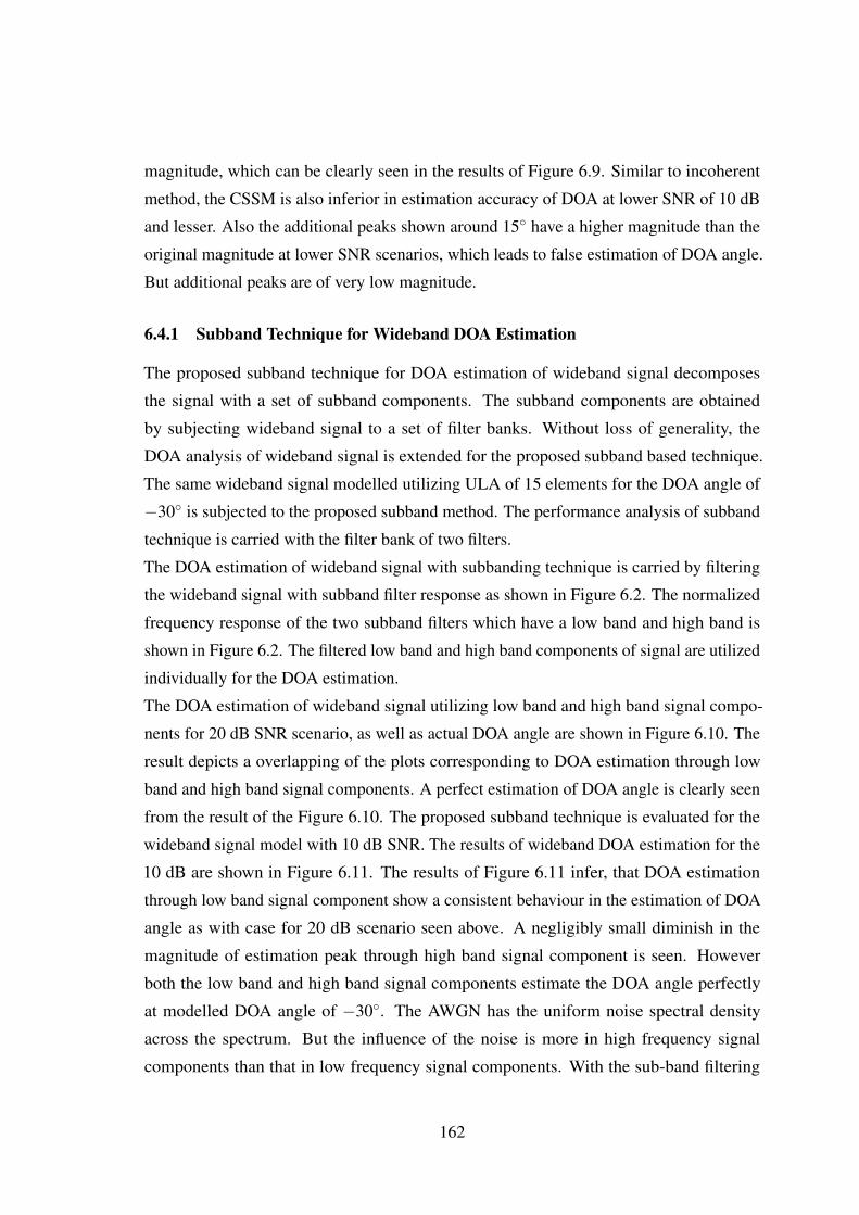
magnitude, which can be clearly seen in the results of Figure 6.9. Similar to incoherent
method, the CSSM is also inferior in estimation accuracy of DOA at lower SNR of 10 dB
and lesser. Also the additional peaks shown around 15◦ have a higher magnitude than the
original magnitude at lower SNR scenarios, which leads to false estimation of DOA angle.
But additional peaks are of very low magnitude.
6.4.1 Subband Technique for Wideband DOA Estimation
The proposed subband technique for DOA estimation of wideband signal decomposes
the signal with a set of subband components. The subband components are obtained
by subjecting wideband signal to a set of filter banks. Without loss of generality, the
DOA analysis of wideband signal is extended for the proposed subband based technique.
The same wideband signal modelled utilizing ULA of 15 elements for the DOA angle of
−30◦ is subjected to the proposed subband method. The performance analysis of subband
technique is carried with the filter bank of two filters.
The DOA estimation of wideband signal with subbanding technique is carried by filtering
the wideband signal with subband filter response as shown in Figure 6.2. The normalized
frequency response of the two subband filters which have a low band and high band is
shown in Figure 6.2. The filtered low band and high band components of signal are utilized
individually for the DOA estimation.
The DOA estimation of wideband signal utilizing low band and high band signal compo-
nents for 20 dB SNR scenario, as well as actual DOA angle are shown in Figure 6.10. The
result depicts a overlapping of the plots corresponding to DOA estimation through low
band and high band signal components. A perfect estimation of DOA angle is clearly seen
from the result of the Figure 6.10. The proposed subband technique is evaluated for the
wideband signal model with 10 dB SNR. The results of wideband DOA estimation for the
10 dB are shown in Figure 6.11. The results of Figure 6.11 infer, that DOA estimation
through low band signal component show a consistent behaviour in the estimation of DOA
angle as with case for 20 dB scenario seen above. A negligibly small diminish in the
magnitude of estimation peak through high band signal component is seen. However
both the low band and high band signal components estimate the DOA angle perfectly
at modelled DOA angle of −30◦. The AWGN has the uniform noise spectral density
across the spectrum. But the influence of the noise is more in high frequency signal
components than that in low frequency signal components. With the sub-band filtering
162
Figure 6.10: Wideband DOA Estimation with Subband Technique with 20 dB SNR
concept, the normalized spectrum is split into two equal halves namely low band and
high band. For the signal modelled with fixed SNR, the low band filter facilitates noise
removal and therefore the influence of the noise is less pronounced on the signals filtered
through low band filter. In the case of high band filter, the noise removal is relatively less
pronounced. The signal filtered with high band filter experiences significant influence
of the noise and it is proportional to the modelled SNR. Therefore the DOA estimation
realised through high frequency band components is prone to relatively higher severity
compared to the estimation obtained through low frequency band components. Thus, the
change in the SNR in signal has not influenced the accuracy of DOA estimate as shown in
Figure 6.11. Further analysis of the subband technique is evaluated for the same wideband
signal model at 5 dB SNR scenario. The corresponding results of subband based DOA
estimation for the 5 dB SNR are depicted in Figure 6.12. The results of DOA estimation
with low band signal component are consistent with the same magnitude and sharpness
of estimation peak along the actual DOA angle as with the case seen in 20 dB and 10 dB
SNR scenario. A significant reduction in the magnitude of the detection peak of estimation
through high band signal component is evident in the results of Figure 6.11. However, even
with the reduced magnitude of peak, the DOA estimation accuracy is still maintained at
the actual DOA of −30◦. The performance of the subband technique is evaluated even
163
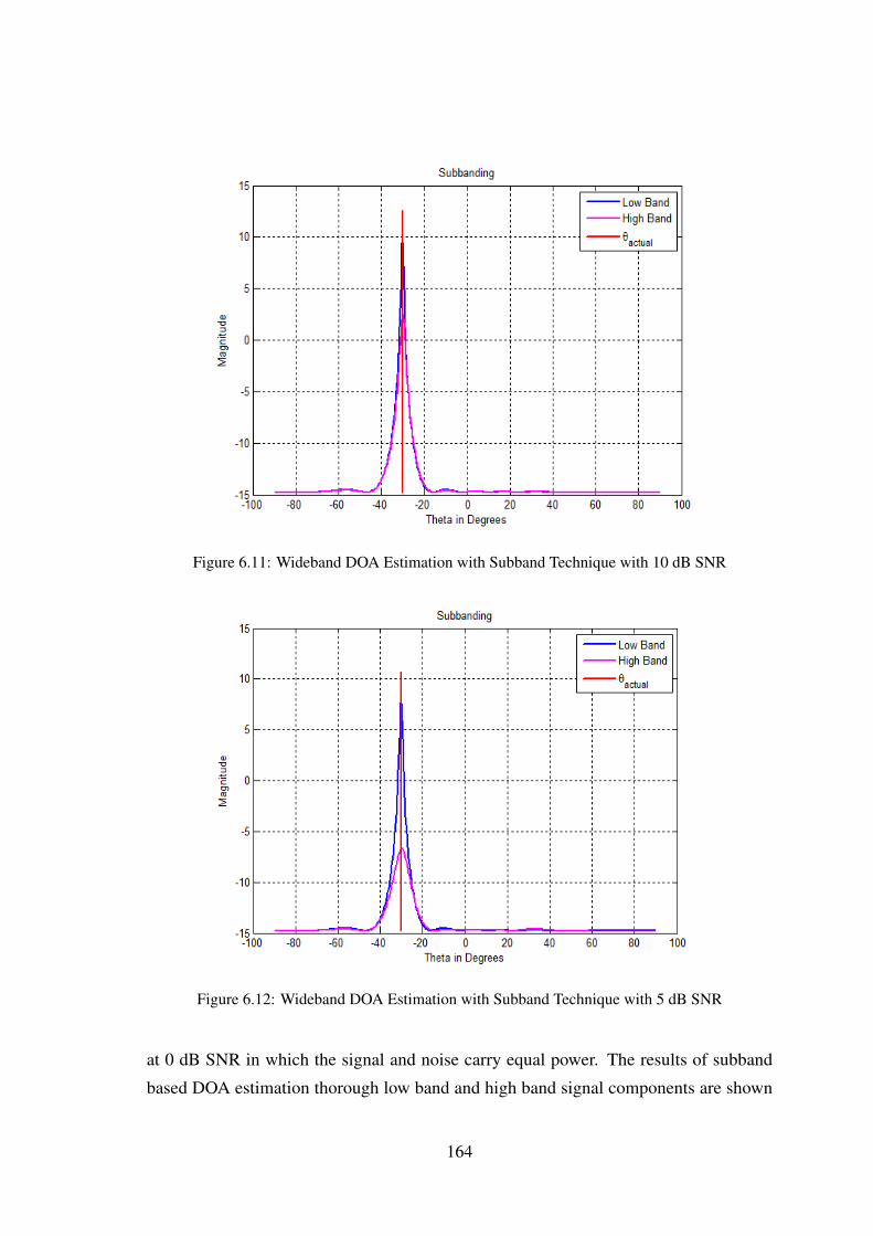
Figure 6.11: Wideband DOA Estimation with Subband Technique with 10 dB SNR
Figure 6.12: Wideband DOA Estimation with Subband Technique with 5 dB SNR
at 0 dB SNR in which the signal and noise carry equal power. The results of subband
based DOA estimation thorough low band and high band signal components are shown
164

in Figure 6.13. The consistent estimate through low band signal component continued
even at 0 dB SNR without losing its large magnitude and sharpness of detection profile
along the actual DOA angle. The estimation through high band signal component exhibits
significantly diminished peak magnitude and also lose its sharpness of peak. The reduced
sharpness of peak leads to degraded estimation accuracy of DOA. The analysis of results
Figure 6.13: Wideband DOA Estimation with Subband Technique with 0 dB SNR
with subband filter based approach of DOA estimate of wideband signal, illustrates that,
the subband based DOA estimation through low band signal component is consistent in the
estimation of DOA through its higher magnitude of detection peak and sharpness along
actual DOA at −30◦. The consistent behaviour is clearly evident at all SNR scenarios.
However the DOA estimation through high band signal component shows diminished
magnitude of detection peak in the estimation at lower SNRs and also loses its sharpness
leading to reduced estimation accuracy. In summary, it can concluded that, only the low
band signal component is sufficient to estimate the DOA of wideband signal at all SNRs.
The high band signal component can be utilized at high and medium range of SNRs and it
cannot be relied upon at very lower SNR scenarios. The average of the DOA estimation
of wideband signal through low band and high band signal components is not preferred
due to the inconsistent nature of the magnitudes of detection peak and sharpness of the
estimations realisable through high band signal components.
165

6.5 Comparison of DOA Estimation Techniques for Wideband Signal
The performance of wideband DOA estimations methods involving the conventional inco-
herent method, coherent signal subspace method and the proposed subbanding techniques
are compared. The results of Figure 6.14 illustrate that the wideband DOA estimation
performance of the three methods at high, medium and lower SNR scenarios. In subband
based technique, only the low band signal component is utilized for the DOA estimation of
wideband signal, since the earlier analysis has proved that it facilitates consistent estimation.
Figure 6.14 shows the comparison of the three methods of DOA estimation for a DOA
Figure 6.14: Comparison of Wideband DOA Estimation with 30 dB SNR
of −30◦. The results of Figure 6.14 reveal the following. The performance of CSSM
and incoherent method of wideband DOA estimation is similar. However, the proposed
subband filtering approach of DOA estimation of wideband signal exhibits much improved
performance. The Figure 6.15 shows the zoomed plot of the peak magnitudes of Figure
6.14. The peak magnitudes of all the three DOA estimation methods of wideband signal
are approximately the same, whereas the incoherent and coherent schemes suffer from
a accuracy of 0.5◦ in DOA estimate at times due to white Gaussian noise present in it.
The results also show the accurate DOA estimation at −30◦ is exhibited by the proposed
subband based technique. The simulation of comparative analysis is further carried for
166

Figure 6.15: Comparison of Wideband DOA Estimation with 30 dB SNR
Figure 6.16: Comparison of Wideband DOA Estimation with 20 dB SNR
wideband signal model with 20 dB SNR scenario. The results corresponding to 20 dB SNR
are shown in Figure 6.16. The results infer that, the DOA estimation through incoherent
167
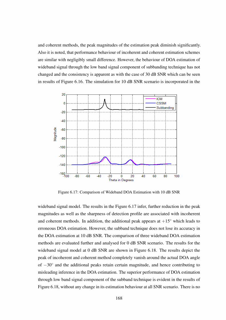
and coherent methods, the peak magnitudes of the estimation peak diminish significantly.
Also it is noted, that performance behaviour of incoherent and coherent estimation schemes
are similar with negligibly small difference. However, the behaviour of DOA estimation of
wideband signal through the low band signal component of subbanding technique has not
changed and the consistency is apparent as with the case of 30 dB SNR which can be seen
in results of Figure 6.16. The simulation for 10 dB SNR scenario is incorporated in the
Figure 6.17: Comparison of Wideband DOA Estimation with 10 dB SNR
wideband signal model. The results in the Figure 6.17 infer, further reduction in the peak
magnitudes as well as the sharpness of detection profile are associated with incoherent
and coherent methods. In addition, the additional peak appears at +15◦ which leads to
erroneous DOA estimation. However, the subband technique does not lose its accuracy in
the DOA estimation at 10 dB SNR. The comparison of three wideband DOA estimation
methods are evaluated further and analysed for 0 dB SNR scenario. The results for the
wideband signal model at 0 dB SNR are shown in Figure 6.18. The results depict the
peak of incoherent and coherent method completely vanish around the actual DOA angle
of −30◦ and the additional peaks retain certain magnitude, and hence contributing to
misleading inference in the DOA estimation. The superior performance of DOA estimation
through low band signal component of the subband technique is evident in the results of
Figure 6.18, without any change in its estimation behaviour at all SNR scenario. There is no
168
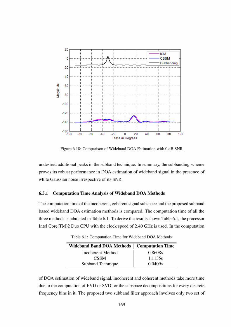
Figure 6.18: Comparison of Wideband DOA Estimation with 0 dB SNR
undesired additional peaks in the subband technique. In summary, the subbanding scheme
proves its robust performance in DOA estimation of wideband signal in the presence of
white Gaussian noise irrespective of its SNR.
6.5.1 Computation Time Analysis of Wideband DOA Methods
The computation time of the incoherent, coherent signal subspace and the proposed subband
based wideband DOA estimation methods is compared. The computation time of all the
three methods is tabulated in Table 6.1. To derive the results shown Table 6.1, the processor
Intel Core(TM)2 Duo CPU with the clock speed of 2.40 GHz is used. In the computation
Table 6.1: Computation Time for Wideband DOA Methods
Wideband Band DOA Methods Computation TimeIncoherent Method 0.8608s
CSSM 1.1135sSubband Technique 0.0409s
of DOA estimation of wideband signal, incoherent and coherent methods take more time
due to the computation of EVD or SVD for the subspace decompositions for every discrete
frequency bins in it. The proposed two subband filter approach involves only two set of
169
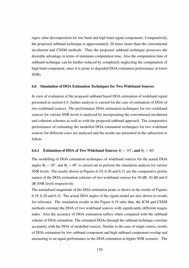
eigen value decomposition for low band and high band signal components. Comparatively,
the proposed subband technique is approximately 20 times faster than the conventional
incoherent and CSSM methods. Thus the proposed subband technique possesses the
desirable advantage in terms of minimum computation time. Also the computation time of
subband technique can be further reduced by completely neglecting the computation of
high band component, since it is prone to degraded DOA estimation performance at lower
SNRs.
6.6 Simulation of DOA Estimation Techniques for Two Wideband Sources
In view of evaluation of the proposed subband based DOA estimation of wideband signal
presented in section 6.5, further analysis is carried for the case of estimation of DOA of
two wideband sources. The performance DOA estimation techniques for two wideband
sources for various SNR levels is analysed by incorporating the conventional incoherent
and coherent schemes as well as with the proposed subband approach. The comparative
performance of estimating the modelled DOA estimation techniques for two wideband
sources for different cases are analysed and the results are presented in the subsection to
follow.
6.6.1 Estimation of DOA of Two Wideband Sources θ1 = 10◦, and θ2 = 40◦
The modelling of DOA estimation techniques of wideband sources for the actual DOA
angles θ1 = 10◦, and θ2 = 40◦ is carried out to perform the simulation analysis for various
SNR levels. The results shown in Figures 6.19, 6.20 and 6.21 are the comparative perfor-
mance of the DOA estimation schemes of two wideband sources for 30 dB, 10 dB and 0
dB SNR levels respectively.
The normalized magnitude of the DOA estimation peaks is shown in the results of Figures
6.19, 6.20 and 6.21. The actual DOA angles of the signal model are also shown in results
for reference. The simulation results in the Figure 6.19 infer that, the ICM and CSSM
methods estimate the DOA of two wideband sources with significantly different magni-
tudes. Also the accuracy of DOA estimation suffers when compared with the subband
scheme of DOA estimation. The estimated DOAs through the subband technique correlate
accurately with the DOA of modelled sources. Similar to the case of single source, results
of DOA estimation by low subband component and high subband component overlap and
amounting to an equal performance in the DOA estimation at higher SNR scenario. The
170
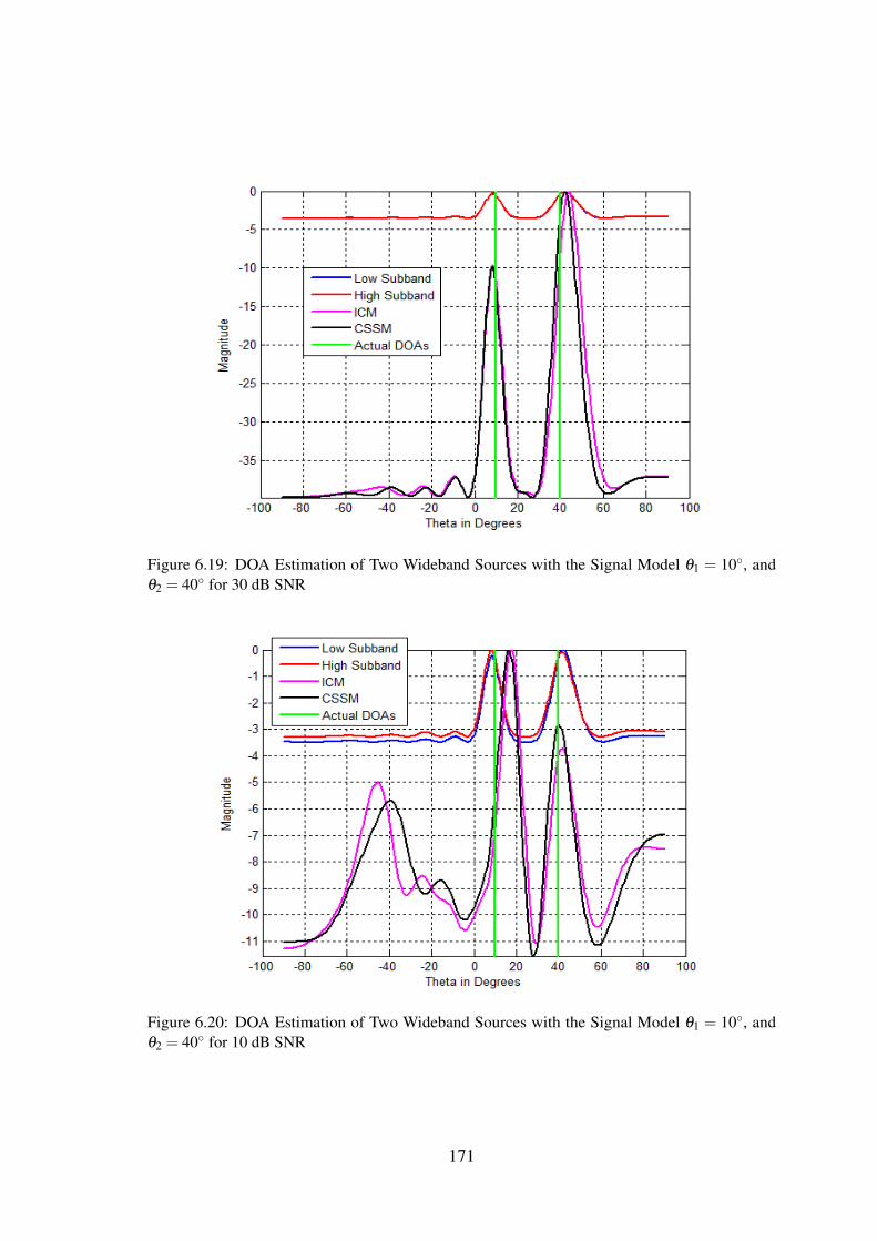
Figure 6.19: DOA Estimation of Two Wideband Sources with the Signal Model θ1 = 10◦, andθ2 = 40◦ for 30 dB SNR
Figure 6.20: DOA Estimation of Two Wideband Sources with the Signal Model θ1 = 10◦, andθ2 = 40◦ for 10 dB SNR
171
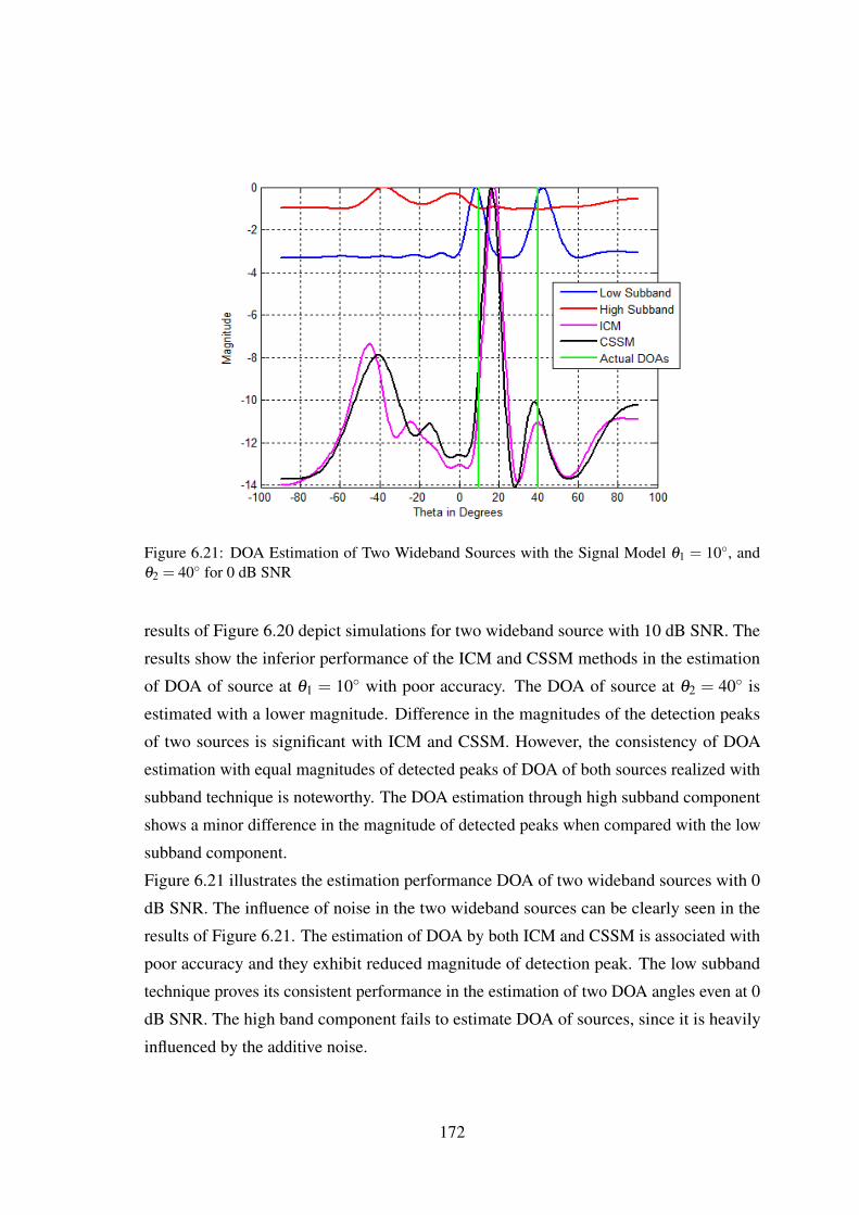
Figure 6.21: DOA Estimation of Two Wideband Sources with the Signal Model θ1 = 10◦, andθ2 = 40◦ for 0 dB SNR
results of Figure 6.20 depict simulations for two wideband source with 10 dB SNR. The
results show the inferior performance of the ICM and CSSM methods in the estimation
of DOA of source at θ1 = 10◦ with poor accuracy. The DOA of source at θ2 = 40◦ is
estimated with a lower magnitude. Difference in the magnitudes of the detection peaks
of two sources is significant with ICM and CSSM. However, the consistency of DOA
estimation with equal magnitudes of detected peaks of DOA of both sources realized with
subband technique is noteworthy. The DOA estimation through high subband component
shows a minor difference in the magnitude of detected peaks when compared with the low
subband component.
Figure 6.21 illustrates the estimation performance DOA of two wideband sources with 0
dB SNR. The influence of noise in the two wideband sources can be clearly seen in the
results of Figure 6.21. The estimation of DOA by both ICM and CSSM is associated with
poor accuracy and they exhibit reduced magnitude of detection peak. The low subband
technique proves its consistent performance in the estimation of two DOA angles even at 0
dB SNR. The high band component fails to estimate DOA of sources, since it is heavily
influenced by the additive noise.
172

6.6.2 Estimation of DOA of Two Wideband Sources θ1 =−10◦, and θ2 = 20◦
The consistent behaviour of the proposed subband based DOA estimation scheme of
wideband signal is evaluated in comparison with incoherent and coherent schemes for
various source angles and SNRs. The two wideband sources are modelled at θ1 =−10◦,
and θ2 = 20◦.
Figure 6.22: DOA Estimation of Two Wideband Sources with the Signal Model θ1 =−10◦, andθ2 = 20◦ for 30 dB SNR
The simulation for the above illustrated scenario and their results of DOA estimations
of wideband signals are provided in the Figures 6.22, 6.23 and 6.24 for the SNR of 30 dB,
10 dB and 0 dB respectively. These results depict, the clear distinction of DOA of two
sources by the estimation through low band component of the subband approach. The high
band component of subband approach fails to perform the estimation of DOA as well as in
distinguishing sources at SNR lower than 10 dB. The coherent and incoherent approaches
estimate the DOA of two sources with significantly different peak magnitudes for SNR of
30 dB and 10 dB. They fail to estimate the DOA of the sources as well as in distinguishing
sources at 0 dB SNR.
173
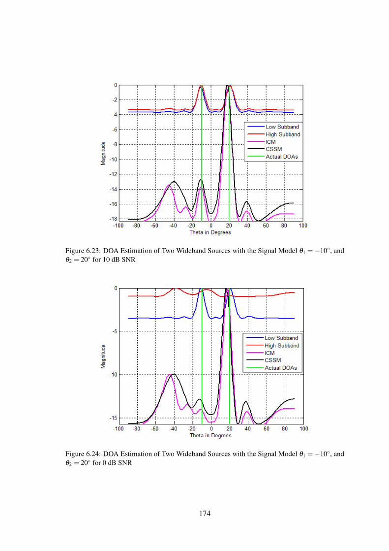
Figure 6.23: DOA Estimation of Two Wideband Sources with the Signal Model θ1 =−10◦, andθ2 = 20◦ for 10 dB SNR
Figure 6.24: DOA Estimation of Two Wideband Sources with the Signal Model θ1 =−10◦, andθ2 = 20◦ for 0 dB SNR
174
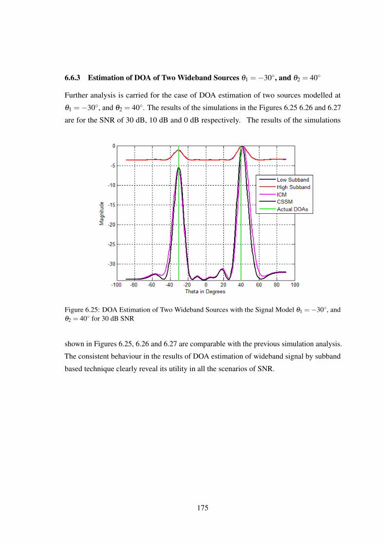
6.6.3 Estimation of DOA of Two Wideband Sources θ1 =−30◦, and θ2 = 40◦
Further analysis is carried for the case of DOA estimation of two sources modelled at
θ1 =−30◦, and θ2 = 40◦. The results of the simulations in the Figures 6.25 6.26 and 6.27
are for the SNR of 30 dB, 10 dB and 0 dB respectively. The results of the simulations
Figure 6.25: DOA Estimation of Two Wideband Sources with the Signal Model θ1 =−30◦, andθ2 = 40◦ for 30 dB SNR
shown in Figures 6.25, 6.26 and 6.27 are comparable with the previous simulation analysis.
The consistent behaviour in the results of DOA estimation of wideband signal by subband
based technique clearly reveal its utility in all the scenarios of SNR.
175

Figure 6.26: DOA Estimation of Two Wideband Sources with the Signal Model θ1 =−30◦, andθ2 = 40◦ for 10 dB SNR
Figure 6.27: DOA Estimation of Two Wideband Sources with the Signal Model θ1 =−30◦, andθ2 = 40◦ for 0 dB SNR
176

6.7 Simulation of 2D-DOA Estimation of Wideband Source by Using Subband Tech-nique
The discussion of the previous section was on the estimation of 1D-DOA of one or more
wideband signals. The 2D-DOA estimation of wideband source using the proposed subband
filter technique is carried to evaluate its performance with the conventional single polarized
array and the proposed orthogonal polarized array configurations in this section.
6.7.1 Wideband Signal Model for 2D-DOA
The 1D signal model for DOA estimation of wideband sources shown in Equation (2.61)
can be extended for the case of 2D-DOA estimation, in which case both the elevation
angle θ and azimuth angle φ are involved in the modelling. For the case of P number of
far-field wideband sources, observed by M antennas arranged in an array geometry with
additive white Gaussian noise, the spectral output of the array of the wideband sources for
frequency f and time sample t is given by the Equations (6.4)
x( f , t) = A( f ,θ ,φ)s( f , t)+n(t) (6.4)
Where A( f ,θ ,φ) is array steering matrix of size P×M, whose columns are spanned by
array steering vector a( f ,θ ,φ) for the frequency f .
x( f , t) =fH
∑i= fL
P
∑p=1
a( fi,θp,φp)sp( fi, t)+n(t) (6.5)
Here the x( f , t) is the observation of wideband signal for frequencies ranging from fL to fH
at time instant t. The signal source s( fi, t) is represented as[s1( f , t), s2( f , t), . . . ,sP( f , t)
]T.
The noise vector n(t) is spectrally and spatially uncorrelated. The noise is also uncorrelated
with the source signals. The array manifold matrix of size M×P can be defined as
A( f ,θ ,φ) =[a( f ,θ1,φ1), a( f ,θ2,φ2), . . . ,a( f ,θP,φP)
](6.6)
The array manifold matrix has the array steering vector a( f ,θp,φp) for the pth source at
frequency f in its columns space. The array steering vector for a elevation angle θ and
azimuth angle φ for case of arbitrary array configuration is defined as
a( f ,θ ,φ) =[e− j 2π f
c β1(θ ,φ), e− j 2π fc β2(θ ,φ), · · · , e− j 2π f
c βM(θ ,φ)]T
(6.7)
Where,
βm (θ ,φ) = xm sinθ cosφ + ym sinθ sinφ + zm cosθ (6.8)
177
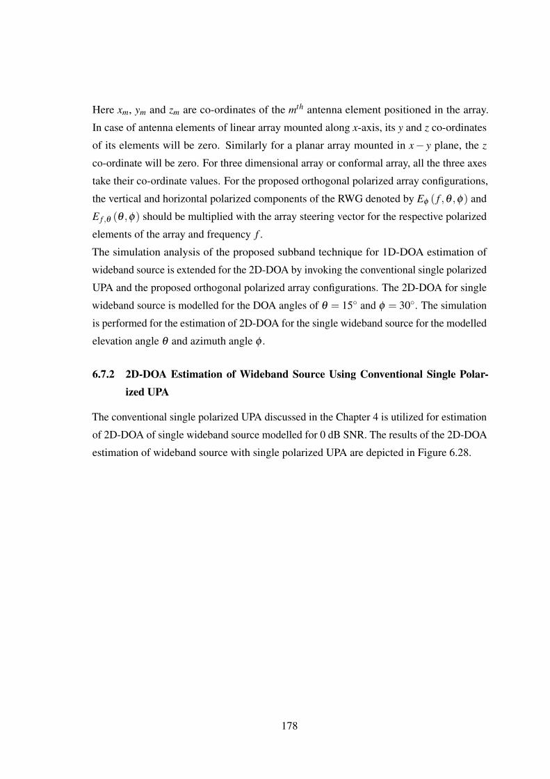
Here xm, ym and zm are co-ordinates of the mth antenna element positioned in the array.
In case of antenna elements of linear array mounted along x-axis, its y and z co-ordinates
of its elements will be zero. Similarly for a planar array mounted in x− y plane, the z
co-ordinate will be zero. For three dimensional array or conformal array, all the three axes
take their co-ordinate values. For the proposed orthogonal polarized array configurations,
the vertical and horizontal polarized components of the RWG denoted by Eφ ( f ,θ ,φ) and
E f ,θ (θ ,φ) should be multiplied with the array steering vector for the respective polarized
elements of the array and frequency f .
The simulation analysis of the proposed subband technique for 1D-DOA estimation of
wideband source is extended for the 2D-DOA by invoking the conventional single polarized
UPA and the proposed orthogonal polarized array configurations. The 2D-DOA for single
wideband source is modelled for the DOA angles of θ = 15◦ and φ = 30◦. The simulation
is performed for the estimation of 2D-DOA for the single wideband source for the modelled
elevation angle θ and azimuth angle φ .
6.7.2 2D-DOA Estimation of Wideband Source Using Conventional Single Polar-ized UPA
The conventional single polarized UPA discussed in the Chapter 4 is utilized for estimation
of 2D-DOA of single wideband source modelled for 0 dB SNR. The results of the 2D-DOA
estimation of wideband source with single polarized UPA are depicted in Figure 6.28.
178
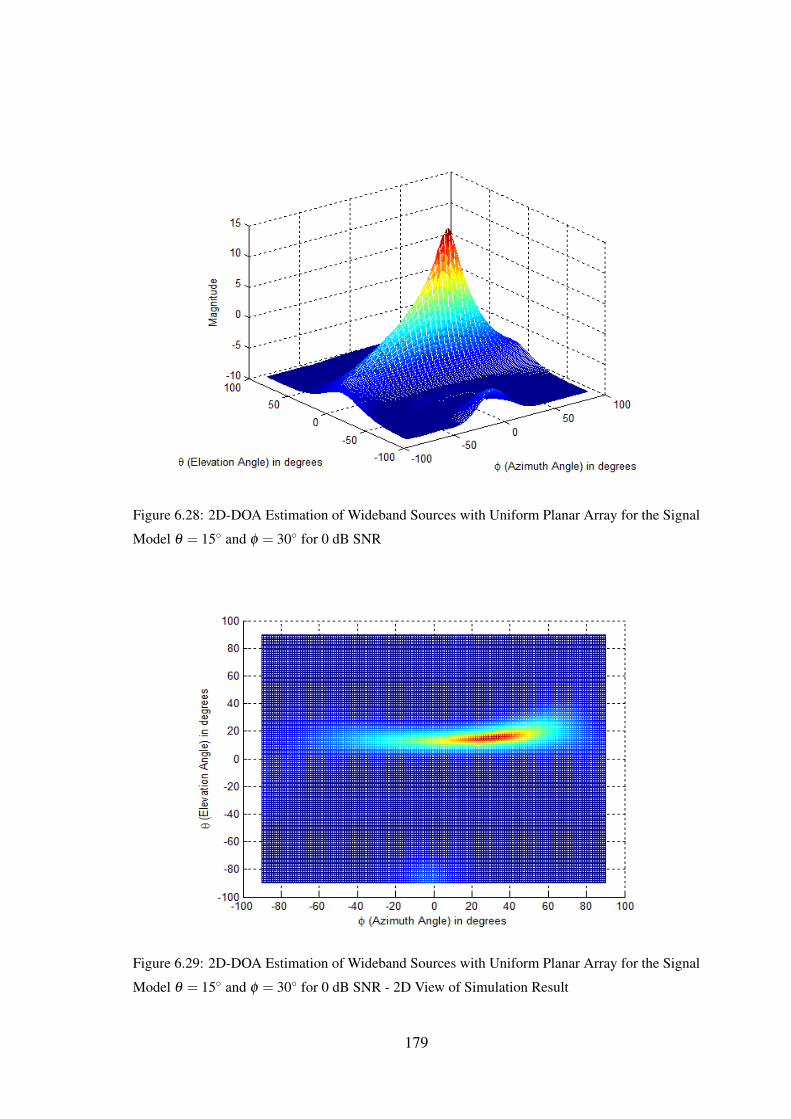
Figure 6.28: 2D-DOA Estimation of Wideband Sources with Uniform Planar Array for the Signal
Model θ = 15◦ and φ = 30◦ for 0 dB SNR
Figure 6.29: 2D-DOA Estimation of Wideband Sources with Uniform Planar Array for the Signal
Model θ = 15◦ and φ = 30◦ for 0 dB SNR - 2D View of Simulation Result
179

The spread of the profile of the detection peak above a certain magnitude can be clearly
seen around the actual DOA angle in the 2D view of the result, depicted in Figure 6.29.
Due to higher noise as well the single polarized array configuration, the performance of
2D-DOA estimation of wideband source with singly polarized UPA is not satisfactory.
6.7.3 2D-DOA Estimation of Wideband Source with OPPA
The performance of 2D-DOA estimation of wideband source with OPPA has been analysed.
The wideband signal model for OPPA configuration is performed for a single source with
angles θ = 15◦ and φ = 30◦.
Figure 6.30: 2D-DOA Estimation of Wideband Sources with Orthogonal Polarized Planar Array for
the Signal Model θ = 15◦ and φ = 30◦ for 0 dB SNR
180
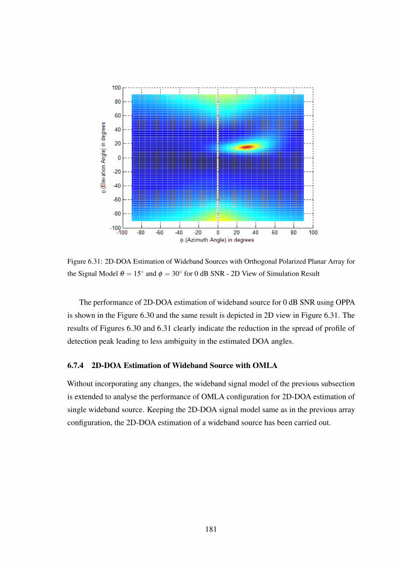
Figure 6.31: 2D-DOA Estimation of Wideband Sources with Orthogonal Polarized Planar Array for
the Signal Model θ = 15◦ and φ = 30◦ for 0 dB SNR - 2D View of Simulation Result
The performance of 2D-DOA estimation of wideband source for 0 dB SNR using OPPA
is shown in the Figure 6.30 and the same result is depicted in 2D view in Figure 6.31. The
results of Figures 6.30 and 6.31 clearly indicate the reduction in the spread of profile of
detection peak leading to less ambiguity in the estimated DOA angles.
6.7.4 2D-DOA Estimation of Wideband Source with OMLA
Without incorporating any changes, the wideband signal model of the previous subsection
is extended to analyse the performance of OMLA configuration for 2D-DOA estimation of
single wideband source. Keeping the 2D-DOA signal model same as in the previous array
configuration, the 2D-DOA estimation of a wideband source has been carried out.
181
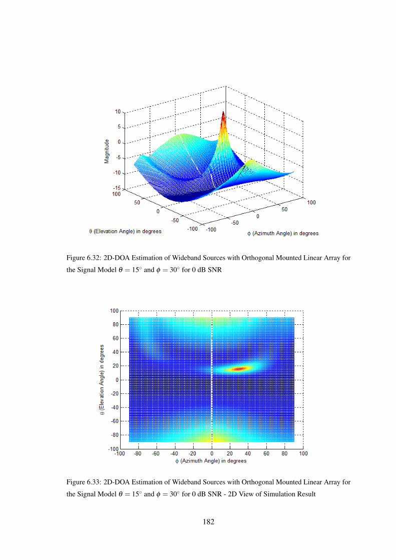
Figure 6.32: 2D-DOA Estimation of Wideband Sources with Orthogonal Mounted Linear Array for
the Signal Model θ = 15◦ and φ = 30◦ for 0 dB SNR
Figure 6.33: 2D-DOA Estimation of Wideband Sources with Orthogonal Mounted Linear Array for
the Signal Model θ = 15◦ and φ = 30◦ for 0 dB SNR - 2D View of Simulation Result
182

The simulation results of 2D-DOA estimation of wideband signal using the OMLA are
shown in Figure 6.32 and the 2D view is depicted in the Figure 6.33. The results of the
simulation of Figures 6.32 and 6.33 confirm that the OMLA facilitates the reduction in the
spread of detection profile leading to improved accuracy of 2D-DOA estimation.
6.7.5 2D-DOA Estimation of Wideband Source with OPLA
The OPLA is also evaluated for its performance in 2D-DOA estimation for the case of
wideband signal scenario. The signal model for single wideband source used in the three
previous array configuration is retained for the simulation. The simulation results of
2D-DOA of wideband signal with OPLA are depicted in Figure 6.34.
Figure 6.34: 2D-DOA Estimation of Wideband Sources with Orthogonal Polarized Linear Array
for the Signal Model θ = 15◦ and φ = 30◦ for 0 dB SNR
183

Figure 6.35: 2D-DOA Estimation of Wideband Sources with Orthogonal Polarized Linear Array
for the Signal Model θ = 15◦ and φ = 30◦ for 0 dB SNR - 2D View of Simulation Result
The result of the simulation are also depicted in 2D view in Figure 6.35. The simulation
results of the OPLA, in which the spread of the detection peak profile is slightly wide. when
compared with the other two orthogonal polarized array configurations. This wider spread
is due to the linear arrangement of the array configuration. In the simulation results of
2D-DOA of single wideband source using the four array configurations discussed, SNR of 0
dB has been considered. It is obvious to expect that the estimation performance of 2D-DOA
using the discussed array configurations will improve with increase in SNR. Appendix B
thus for to presents additional results of 2D-DOA estimation of single wideband source
at higher SNR values using various array configurations. It is clearly evident from the
simulation results, the orthogonal polarized array configuration is helpful in improving the
2D-DOA estimation of wideband signals with improved accuracy when compared to the
conventional single polarized UPA.
184

6.7.6 RMSE Performance Analysis of Subband Based 2D-DOA Estimation of Wide-band Signal with Single and Orthogonal Polarized Array Configurations
From the analysis of simulation results of the previous subsections, it is clear that the
proposed wideband DOA estimation scheme based on subband filter exhibits consistency
and superiority in the 1D-DOA estimation in all SNR scenarios. This subbanding technique
is further analysed for its RMSE performance for the range of SNRs using the conventional
single and the proposed orthogonal polarized array configurations. The wideband signal
model for the conventional single polarized UPA and the proposed orthogonal polarized
array configurations namely, OPPA, OMLA and OPLA modelled in the previous subsec-
tions is used for RMSE analysis. The DOA for the wideband signal model is carried for
θ = 15◦ and φ = 30◦. This wideband signal model is subjected for the analysis invoking
the proposed subbanding technique for the wideband 2D-DOA estimation at 0 to 30 dB
SNR scenarios. As per the previous analysis, the low band signal component for the
estimation of DOA of the wideband source is utilized and the estimation through high band
signal components is ignored in the simulation.
Figure 6.36: RMSE Comparison for θ Angle Estimation of 2D-DOA Estimation of Wideband
Signal for Single and Orthogonal Polarized Array Configurations
185

Figure 6.37: RMSE Comparison for φ Angle Estimation of 2D-DOA Estimation of Wideband
Signal for Single and Orthogonal Polarized Array Configurations
The RMSE performance of DOA estimation of wideband signal for both the θ and φ
angles of 2D-DOA is analysed for 0 to 30 dB SNR scenarios. The results of the RMSE
performance of θ and φ angles of 2D-DOA estimations are illustrated in Figures 6.36 and
6.37 respectively. Comparison of the wideband estimation performance is seen individually
for the elevation angle θ and the azimuth angle φ estimations for the single and orthogonal
polarizes array configurations. The analysis of influence of array configuration on the
2D-DOA estimation presented in the previous chapters for narrow band cases and tracking
performances has been extended for the case of wideband sources also. At lower SNR, the
estimation of φ angle is less accurate when compared to the estimation ofθ angle. The
single polarized UPA configuration is more prone for error in the estimation of azimuth
φ angle, when compared to the proposed orthogonal array configurations. The OMLA
and OPPA configurations are better in their performance. These two array configurations
show almost similar performance with least RMSE in their θ and φ angle estimation. The
OPLA suffers slightly due to its linear geometric arrangement in the 2D-DOA estimation.
However OPLA shows improved DOA estimation of wideband source when compared
with the azimuth angle φ estimation of conventional single polarized UPA configuration.
186

6.8 Simulation of 2D-DOA Estimation of Two Wideband Source by Using SubbandTechnique
The simulation analysis of the proposed subband technique for DOA of wideband source is
further extended for the 2D-DOA of two wideband sources. The two wideband incoming
sources and the estimation of 2D-DOA are carried by invoking the conventional single
polarized UPA and the proposed orthogonal polarized arrays. The 2D-DOA for two
wideband sources are modelled for the DOA angles (θ1 = 52◦ , φ1 = 28◦) and (θ2 = 40◦ ,
φ2 = 65◦).
6.8.1 2D-DOA Estimation of Two Wideband Sources with Conventional Single Po-larized UPA
The conventional single polarized UPA discussed in the previous chapters is utilized for
estimation of 2D-DOA of two wideband sources modelled for 0 dB SNR. The results of the
2D-DOA estimation with single polarized UPA are shown in Figure 6.38. The magnitudes
of detection peaks corresponding to 2D-DOA of two sources are different. Additional
fictitious peak is also seen in the results leading to ambiguity in the estimation of 2D-DOA.
Figure 6.38: 2D-DOA Estimation of Two Wideband Sources with Uniform Planar Array for the
Signal Model (θ1 = 52◦ , φ1 = 28◦) and (θ2 = 40◦ , φ2 = 65◦) for 0 dB SNR
187

Figure 6.39: 2D-DOA Estimation of Two Wideband Sources with Uniform Planar Array for the
Signal Model (θ1 = 52◦ , φ1 = 28◦) and (θ2 = 40◦ , φ2 = 65◦) for 0 dB SNR - 2D View of
Simulation Result
A spread of peak magnitudes around the DOA of the two modelled wide band sources
are seen in results of Figure 6.39. The additional peak at angle (−50◦,−30◦) is a spurious
peak. The availability of only single polarized component, uniform covariance of the
received data as well as the lack of provision for further reduction of inter-element spacing
induce the additional spurious peak in the estimation. Also, the results of the simulation at
higher SNR also confirm that the magnitude of spurious peak is not reducing. The results
of 2D-DOA estimation at higher SNR scenario are shown in Figures C.1, C.2, C.3, C.4,
C.5 and C.6 of Appendix C.
6.8.2 2D-DOA Estimation of Two Wideband Sources with OPPA
The proposed OPPA configuration is evaluated for its performance in estimating the 2D-
DOA of two wideband sources. The results of the 2D-DOA estimation with two wideband
sources are presented in Figure 6.40 for 0 dB SNR.
188

Figure 6.40: 2D-DOA Estimation of Two Wideband Sources with Orthogonal Polarized Planar
Array for the Signal Model (θ1 = 52◦ , φ1 = 28◦) and (θ2 = 40◦ , φ2 = 65◦) for 0 dB SNR
Figure 6.41: 2D-DOA Estimation of Two Wideband Sources with Orthogonal Polarized Planar
Array for the Signal Model (θ1 = 52◦ , φ1 = 28◦) and (θ2 = 40◦ , φ2 = 65◦) for 0 dB SNR - 2D
View of Simulation Result
189
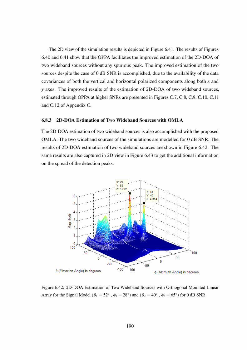
The 2D view of the simulation results is depicted in Figure 6.41. The results of Figures
6.40 and 6.41 show that the OPPA facilitates the improved estimation of the 2D-DOA of
two wideband sources without any spurious peak. The improved estimation of the two
sources despite the case of 0 dB SNR is accomplished, due to the availability of the data
covariances of both the vertical and horizontal polarized components along both x and
y axes. The improved results of the estimation of 2D-DOA of two wideband sources,
estimated through OPPA at higher SNRs are presented in Figures C.7, C.8, C.9, C.10, C.11
and C.12 of Appendix C.
6.8.3 2D-DOA Estimation of Two Wideband Sources with OMLA
The 2D-DOA estimation of two wideband sources is also accomplished with the proposed
OMLA. The two wideband sources of the simulations are modelled for 0 dB SNR. The
results of 2D-DOA estimation of two wideband sources are shown in Figure 6.42. The
same results are also captured in 2D view in Figure 6.43 to get the additional information
on the spread of the detection peaks.
Figure 6.42: 2D-DOA Estimation of Two Wideband Sources with Orthogonal Mounted Linear
Array for the Signal Model (θ1 = 52◦ , φ1 = 28◦) and (θ2 = 40◦ , φ2 = 65◦) for 0 dB SNR
190

Figure 6.43: 2D-DOA Estimation of Two Wideband Sources with Orthogonal Mounted Linear
Array for the Signal Model (θ1 = 52◦ , φ1 = 28◦) and (θ2 = 40◦ , φ2 = 65◦) for 0 dB SNR - 2D
View of Simulation Result
The results of Figure 6.42 reveal the higher magnitudes of detection peaks. The OMLA
has limited covariance data of both the horizontal and vertical polarized components in
both the x and y axes. In addition, the wideband nature of the two sources at 0 dB SNR,
the spurious peaks of Figure 6.42 with reduced magnitudes than the peaks corresponding
to the actual DOA of sources can be seen in the results. However, the magnitude of these
spurious peak diminish as SNR of the data covariances increases. The results of diminishing
magnitude of spurious peaks at higher SNRs can be seen in the results presented Figures
C.13, C.14, C.15, C.16, C.17 and C.18 in Appendix C.
6.8.4 2D-DOA Estimation of Two Wideband Sources with OPLA
The simulation of 2D-DOA estimation is also carried for the proposed OPLA, keeping the
same DOA angles of the source modelling. The estimation performance of 2D-DOA with
OPLA as well as the corresponding detection peak and the spread of profile of detection
peak can be seen in the results of Figure 6.44 and 6.45 respectively.
191
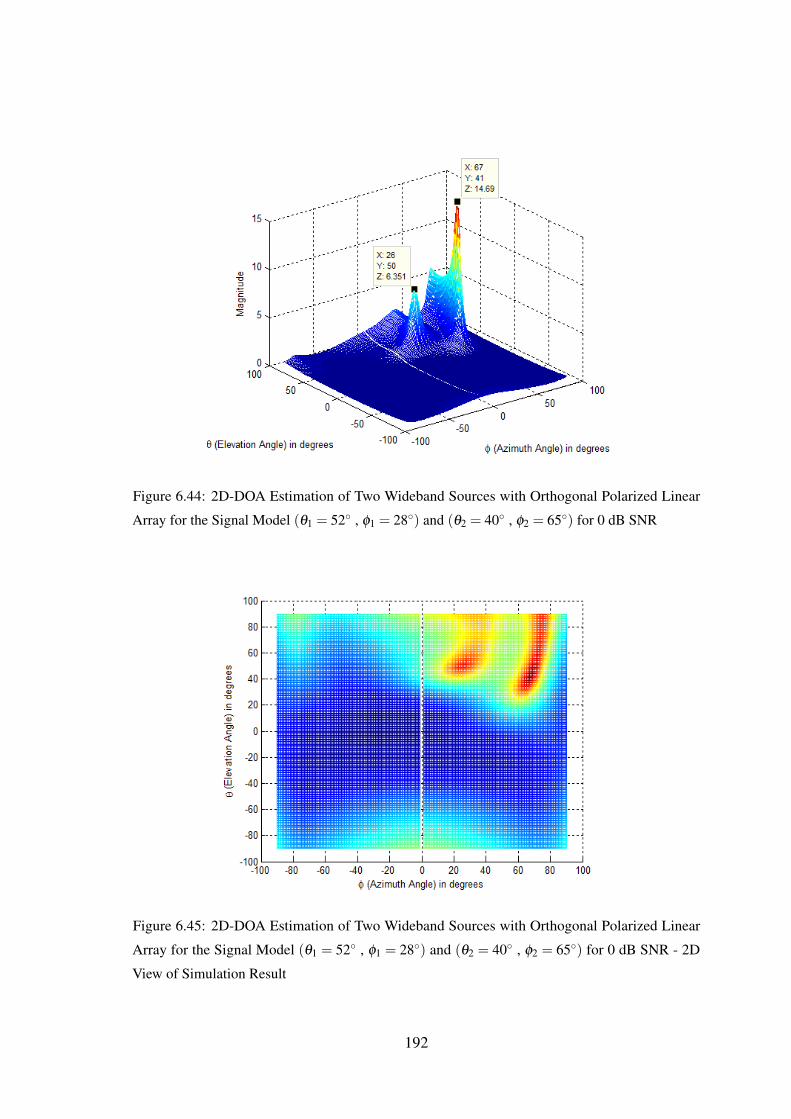
Figure 6.44: 2D-DOA Estimation of Two Wideband Sources with Orthogonal Polarized Linear
Array for the Signal Model (θ1 = 52◦ , φ1 = 28◦) and (θ2 = 40◦ , φ2 = 65◦) for 0 dB SNR
Figure 6.45: 2D-DOA Estimation of Two Wideband Sources with Orthogonal Polarized Linear
Array for the Signal Model (θ1 = 52◦ , φ1 = 28◦) and (θ2 = 40◦ , φ2 = 65◦) for 0 dB SNR - 2D
View of Simulation Result
192
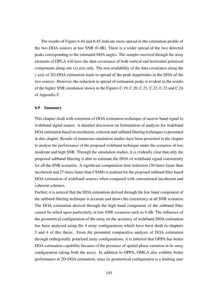
The results of Figure 6.44 and 6.45 indicate more spread in the estimation profile of
the two DOA sources at low SNR (0 dB). There is a wider spread of the two detected
peaks corresponding to the estimated DOA angles. The samples received through the array
elements of OPLA will have the data covariance of both vertical and horizontal polarized
components along one (x) axis only. The non-availability of the data covariance along the
y axis of 2D-DOA estimation leads to spread of the peak magnitudes in the DOA of the
two sources. However, the reduction in spread of estimation peaks is evident in the results
of the higher SNR simulation shown in the Figures C.19, C.20, C.21, C.22, C.23 and C.24
of Appendix C.
6.9 Summary
This chapter dealt with extension of DOA estimation technique of narrow band signal to
wideband signal source. A detailed discussion on formulation of analysis for wideband
DOA estimation based on incoherent, coherent and subband filtering techniques is presented
in this chapter. Results of numerous simulation studies have been presented in the chapter
to analyse the performance of the proposed wideband technique under the scenarios of low,
moderate and high SNR. Through the simulation studies, it is evidently clear that only the
proposed subband filtering is able to estimate the DOA of wideband signal consistently
for all the SNR scenarios. A significant computation time reduction (20 times faster than
incoherent and 27 times faster than CSSM) is realized for the proposed subband filter based
DOA estimation of wideband sources when compared with conventional incoherent and
coherent schemes.
Further, it is noticed that the DOA estimation derived through the low band component of
the subband filtering technique is accurate and shows the consistency at all SNR scenarios.
The DOA estimation derived through the high band component of the subband filter
cannot be relied upon particularly at low SNR scenarios such as 0 dB. The influence of
the geometrical configuration of the array on the accuracy of wideband DOA estimation
has been analysed using the 4 array configurations which have been dealt in chapters
3 and 4 of this thesis. From the presented comparative analysis of DOA estimation
through orthogonally polarized array configurations, it is inferred that OPPA has better
DOA estimation capability because of the presence of spatial phase variation in its array
configuration (along both the axes). In addition to OPPA, OMLA also exhibits better
performance in 2D-DOA estimation, since its geometrical configuration is a limiting case
193

of OPPA. The performance of the 2D-DOA of wideband sources with OPPA has been
found to be more accurate and consistent for various simulation scenarios.
194

Chapter 7
Conclusions
This chapter intends to summarize and facilitate recapitulation of succinct summary,
inferences, technical conclusions derived out of the undertaken research study of this thesis.
The potential avenues for further explorations and investigations of the research study
presented in this thesis are also emphasised.
7.1 Research Summary
The topic of parameter estimation has attracted many researchers over the past several
decades. The estimation of the parameter DOA and its multi disciplinary approach pose
challenges to RF and signal processing engineers. The estimation of DOA of electromag-
netic sources continues to warrant the performance improvement of the DOA estimation
algorithms dealing with single and multiple sources. In addition, there is a greater emphasis
for tracking of DOA of dynamic sources. There is growing need to extend the DOA
estimation algorithms established for narrow band sources to wideband sources. There
is always a desirable need to minimize the computational complexity of proven DOA
algorithms without compromising the accuracy and reliability.
In this context, this research was motivated towards the utilization of orthogonal polarized
antenna array configurations for the improvement of accuracy and resolution of DOA
estimation invoking the classical MUSIC algorithm. By utilizing orthogonal polarized
elements of the antenna array, a closed form solution was derived for the estimation of
2D-DOA with 1D search technique to realize reduced computation complexity. This thesis
proposes novel orthogonally polarized array configurations to facilitate enhanced accuracy
and resolution of 2D-DOA estimation algorithms for single and multiple sources. The
novel orthogonal polarized array configurations include OPLA, OPPA and OMLA.
The improved capability of distinguishing two closely spaced sources is realized with
the proposed orthogonal polarized arrays when compared to single polarized UPA con-
figuration. This thesis also analysed the proposed array configurations for their potential
195
in tracking of 2D-DOA of sources. The combination of orthogonally polarized array
configurations and the conventional MUSIC algorithm is extended to analyse the tracking
behaviour of 2D-DOA estimation of dynamic sources. Further, this thesis also covered
the development of 1D and 2D-DOA estimation of wideband sources using the proposed
orthogonally polarized array configurations. A novel subbanding technique for wideband
DOA technique was proposed and its improved performance was substantiated through a
comparative study involving conventional algorithms for estimation of DOA of wideband
sources.
7.2 Conclusions
The technical observations, inferences, original contributions and conclusions of this
research are briefly reviewed in the following subsections.
7.2.1 Formulation of Closed Form solution for 2D-DOA Estimation with OPLA
Formulation of an analysis to derive the closed form expression for the estimation of
2D-DOA of a single source using the linear array configuration constituted the primary
theme of the 3rd chapter of this thesis. Under the purview of this topic, the following
conclusions can be derived from the simulation studies.
• The OPLA configuration can be used to estimate the DOA with classical subspace
based MUSIC algorithm. The derived closed form expression can be used along
with the classical subspace based technique to estimate the 2D-DOA. The search
dimensions are reduced from 2D to 1D thereby minimizing the computational
complexity involved in 2D-DOA estimation.
• The derived solution estimates both azimuth and elevation angles of distant sources
utilizing a linear array configuration. The proposed one-dimensional search is a
consequence of utilizing the linear array configuration with its alternate elements
orthogonally polarized.
• The distinct feature of the proposed one-dimensional search technique leading to a
significant reduction in the computation time for two-dimensional DOA estimation
using MUSIC algorithm has been illustrated through the simulation studies.
196

• The proposed formulation can be extended to any other antenna whose radiation
pattern can be represented through an analytical expression involving separable form
of elevation angle θ and azimuth angle φ .
• Simulation results of 2D-DOA obtained with conventional single polarized UPA (2×2) have been correlated with those obtained through OPLA and very good correlation
exists between the results of the above two array configurations. The proposed
one-dimensional search technique has resulted in an acceleration of computation
time by factors of 50 and 150 for 1◦ and 0.5◦ search intervals respectively.
7.2.2 2D-DOA Estimation with Orthogonal Polarized Arrays
Formulation of an analysis to estimate the 2D-DOA of multiple sources with enhanced
accuracy and improved resolution is the main focus of the 4th chapter of this thesis.
• The simulations and analysis have been carried out to confirm that the orthogonally
polarized elements of antenna array have significant influence in the accuracy and
resolution of the estimation of 2D-DOA.
• The proposed OPLA as a physical arrangement can be treated as a linear array. Thus
a linear array configuration and its ability to estimate the 2D-DOA is the novel part
of the proposed OPLA.
• The proposed configuration of OPPA has improved accuracy of estimation of 2D-
DOA when compared with single polarized UPA.
• The proposed OMLA configuration estimates the two DOA sources with higher
magnitudes when compared with the other proposed orthogonally polarized and
conventional UPA configuration.
• The improved capability of the orthogonally polarized arrays in distinguishing the
closely spaced sources is also substantiated through the simulation studies.
• The OPPA and the OMLA clearly distinguish the DOA of sources with minimum
angular separation of 10◦. The conventional single polarized UPA configuration
could resolve the two sources whose angular separation was 18◦ or more, which is
inferior when compared with the proposed OPPA and OMLA configurations.
197

• The orthogonally polarized linear elements resolve DOA of the two sources with
angular separation of 10◦ with increased inter-element spacing.
• The consistent accurate estimation of the 2D-DOA for two sources and three sources
under high, medium and low SNR scenario with the proposed orthogonally polarized
array configurations and the derivable higher resolution have been substantiated from
the simulation analysis.
7.2.3 Orthogonal Polarized Arrays for Tracking of 2D-DOA for Dynamic Sources
The primary emphasis of the 5th chapter of this thesis has been the extension of the analysis
of the orthogonally polarized array configurations to track the 2D-DOA of dynamic sources
using different schemes of formation of covariance matrix.
• The simulation analysis of tracking behaviour of 2D-DOA with the conventional
single polarized and orthogonal polarized array configurations has been carried out.
The tracking behaviour of 2D-DOA estimation algorithms is analysed by comparing
the computed MSE between true trajectory and estimated trajectory.
• The MSE for θ and φ angles of tracking the estimation of 2D-DOA is computed by
utilizing the different approaches in the formation of data covariance matrix such as
instantaneous samples approach, weighting factor and forgetting factor approaches.
• The results of the analysis are tabulated for the low, medium and high SNR scenarios
in the Table 5.1. The comparative analysis reveals, that the OPPA outperforms the
other array configurations with least MSE in the 2D-DOA estimation and as well as
in tracking of 2D-DOA estimation.
• The OMLA performs better, when compared to UPA and OPLA configurations.
• The OPLA performs almost equally with UPA at medium and high SNR scenarios.
Due to the linear geometric configuration, the OPLA shows, a small degradation in
θ estimations when compared to UPA at low SNR.
• The forgetting factor approach in the covariance matrix formation tracks the 2D-DOA
estimation more accurately when compared to instantaneous samples and weighting
factor approaches.
198
7.2.4 Subband Filter Technique for DOA Estimation of Wideband Sources
The various analytical and simulation studies on DOA estimation of narrow band sources
have been extended to the scenario of wideband signal too. The conclusions derived from
the pertinent simulation studies on the estimation of 2D-DOA of wideband sources are
presented in this subsection.
• The subband filter approach for DOA estimation of wideband source is proposed
and the performance of estimation of DOA of the proposed approach has been
compared with conventional wideband DOA estimation methods namely incoherent
and coherent signal subspace methods.
• The comparative analysis of the proposed subband filter based wideband DOA
estimation scheme outperforms the conventional incoherent and coherent signal
subspace method.
• A significant reduction in computation time (20 times faster than incoherent and
27 times faster than CSSM) is realized for the proposed subband filter based DOA
estimation of wideband sources.
• The proposed two subband filter approach yields the DOA estimation through the
two components namely low band and high band signals. The estimation of DOA
derived through the signal component of low band exhibits satisfactory performance
in low, medium and high SNR scenarios including the case of 0 dB.
• The accuracy of the estimation of DOA of wideband signal through incoherent
and coherent methods as well as through the high band signal of the subband filter
approach is satisfactory only in high SNR. However they have the limitation of
degraded performance in low and medium SNR cases.
• Among the various array configurations used in the estimation of DOA of wideband
sources, the OPPA and OMLA exhibit the feature of improved estimation through
low RMSE even in low SNR scenario.
• The performance analysis of DOA estimation of two wideband signals has also
been carried out using the proposed subband filter approach and the simulation
results reveal the relative performance improvement compared to the conventional
incoherent and coherent subspace methods.
199
• The accuracy of 2D-DOA estimation of wideband sources obtained through the
signal component of low band is consistently better when compared to the other
approaches cited above and the relative performance accuracy is significantly higher
particularly in medium and low SNR scenarios.
• The conventional single polarized UPA exhibits spurious peaks at an arbitrary DOA
angle which tend to mislead the DOA estimation, whereas the proposed orthogonal
array configurations estimate the DOA angles of the sources without spurious peaks.
• The orthogonally polarized array configurations proposed in this thesis continue
to facilitate better performance of the 2D-DOA estimation of two wideband signal
sources.
7.3 Contributions
The following are the contributions of this thesis whose emphasis is on the estimation and
tracking of 2D-DOA applying MUSIC algorithm.
• Derivation of the closed form expression for the estimation of 2D-DOA of a single
source using the orthogonally polarized linear array configuration.
• Novel orthogonal polarized array configurations for improved accuracy and resolu-
tion estimation of 2D-DOA.
• Improved tracking accuracy of 2D-DOA estimation by utilizing orthogonal polarized
array configurations as well as forgetting factor approach based covariance matrix.
• Enhanced accuracy in estimation of 2D-DOA of wideband sources by invoking
subband filter approach.
7.4 Suggestions for Future Work
Research is a voyage of discovery. It is a path for unknown to the known and at times,
known to the unknown. The philosophy of research always provides impetus to look for
avenues to enhance the scope of current state of knowledge and understanding of any topic
of interest to research community. With these words, potential avenues to further advance
the research topic of this thesis are highlighted.
200
7.4.1 Orthogonal Polarized Arrays
• Like the rectangular waveguides as antenna, chosen in this thesis, other potential
waveguides and antenna elements suitable to be applied for DOA estimation can be
explored for their utility in orthogonal polarized array configuration for estimation
of 2D-DOA.
• Invoking dual polarized antenna elements for DOA estimation by simultaneous
reception of both the horizontal and vertical polarized components might yield
novelty as well as paving the way for a new direction in modelling of antenna arrays
and signal processing algorithms.
• Analysis to investigate the influence of mutual coupling of the various array configu-
rations proposed in this thesis is yet to be formalised and the same can constitute a
significant part for the future work.
7.4.2 Tracking of 2D-DOA
• The repeated computation of SVD during the tracking of 2D-DOA can be cir-
cumvented by the Bi-SVD and modified Bi-SVD algorithms for reduction in the
computation complexity.
• An implicit assumption of linear movement of the DOA sources is associated with the
research of this thesis. However, tracking of estimation of 2D-DOA with non-linear
movements of non-stationary signal sources is worth pursuing further.
• The extraction of DOA information and tracking the estimation of DOA in the
presence of non-linear movements of single and multiple signal sources in a dynamic
changing environment pose significant challenges in the estimation algorithm.
• A forgetting factor based smoothing of covariance data matrix is carried out in
this thesis. Further a prediction based tracking algorithm for linear and non-linear
movements of non-stationary DOA sources can be analysed by invoking Kalman
Filter and Extended Kalman Filter based techniques.
• A Gaussian white noise process is utilized for the simulation analysis in most of this
thesis. Instead consideration of a non-Gaussian noise with non-linearity in the signal
model is a worth while exercise of practical significance.
201

7.4.3 Wideband DOA Estimation Techniques
• The proposed two subband approaches can be extended to multiple filter bank
approach for further improvements in estimation of DOA of wideband sources.
• The polyphase decomposition scheme in the multirate filter bank approaches may
offer potential scope for improvements in the estimation of DOA of wideband
sources.
• The Short Time Fourier Transform (STFT), Wavelet Filters and Gabor Filters can
also be incorporated in estimation of DOA of wideband sources.
202
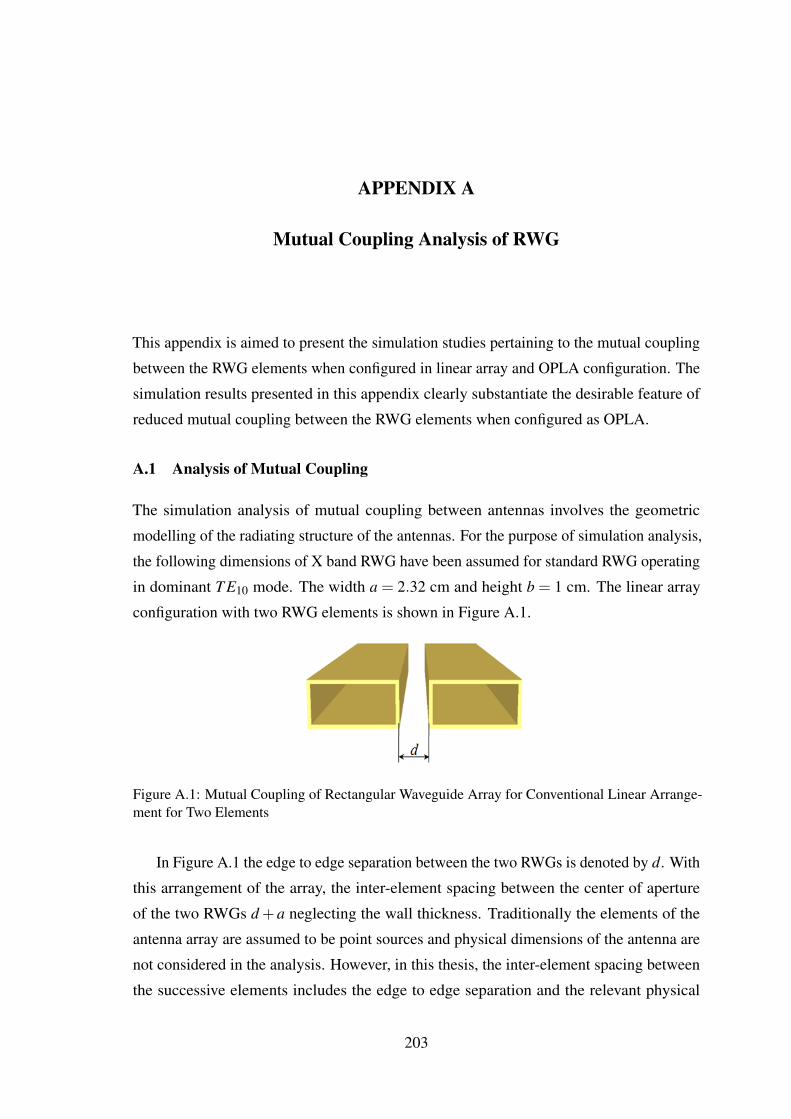
APPENDIX A
Mutual Coupling Analysis of RWG
This appendix is aimed to present the simulation studies pertaining to the mutual coupling
between the RWG elements when configured in linear array and OPLA configuration. The
simulation results presented in this appendix clearly substantiate the desirable feature of
reduced mutual coupling between the RWG elements when configured as OPLA.
A.1 Analysis of Mutual Coupling
The simulation analysis of mutual coupling between antennas involves the geometric
modelling of the radiating structure of the antennas. For the purpose of simulation analysis,
the following dimensions of X band RWG have been assumed for standard RWG operating
in dominant T E10 mode. The width a = 2.32 cm and height b = 1 cm. The linear array
configuration with two RWG elements is shown in Figure A.1.
Figure A.1: Mutual Coupling of Rectangular Waveguide Array for Conventional Linear Arrange-ment for Two Elements
In Figure A.1 the edge to edge separation between the two RWGs is denoted by d. With
this arrangement of the array, the inter-element spacing between the center of aperture
of the two RWGs d +a neglecting the wall thickness. Traditionally the elements of the
antenna array are assumed to be point sources and physical dimensions of the antenna are
not considered in the analysis. However, in this thesis, the inter-element spacing between
the successive elements includes the edge to edge separation and the relevant physical
203
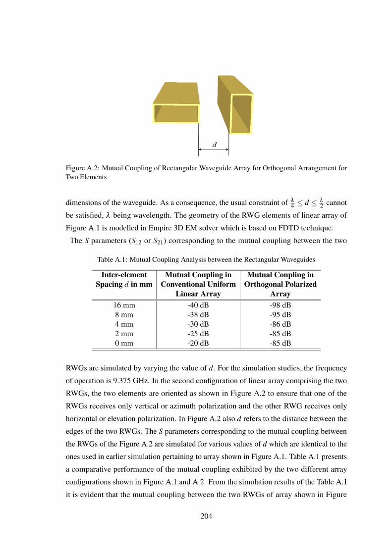
Figure A.2: Mutual Coupling of Rectangular Waveguide Array for Orthogonal Arrangement forTwo Elements
dimensions of the waveguide. As a consequence, the usual constraint of λ
4 ≤ d ≤ λ
2 cannot
be satisfied, λ being wavelength. The geometry of the RWG elements of linear array of
Figure A.1 is modelled in Empire 3D EM solver which is based on FDTD technique.
The S parameters (S12 or S21) corresponding to the mutual coupling between the two
Table A.1: Mutual Coupling Analysis between the Rectangular Waveguides
Inter-element Mutual Coupling in Mutual Coupling inSpacing d in mm Conventional Uniform Orthogonal Polarized
Linear Array Array16 mm -40 dB -98 dB8 mm -38 dB -95 dB4 mm -30 dB -86 dB2 mm -25 dB -85 dB0 mm -20 dB -85 dB
RWGs are simulated by varying the value of d. For the simulation studies, the frequency
of operation is 9.375 GHz. In the second configuration of linear array comprising the two
RWGs, the two elements are oriented as shown in Figure A.2 to ensure that one of the
RWGs receives only vertical or azimuth polarization and the other RWG receives only
horizontal or elevation polarization. In Figure A.2 also d refers to the distance between the
edges of the two RWGs. The S parameters corresponding to the mutual coupling between
the RWGs of the Figure A.2 are simulated for various values of d which are identical to the
ones used in earlier simulation pertaining to array shown in Figure A.1. Table A.1 presents
a comparative performance of the mutual coupling exhibited by the two different array
configurations shown in Figure A.1 and A.2. From the simulation results of the Table A.1
it is evident that the mutual coupling between the two RWGs of array shown in Figure
204
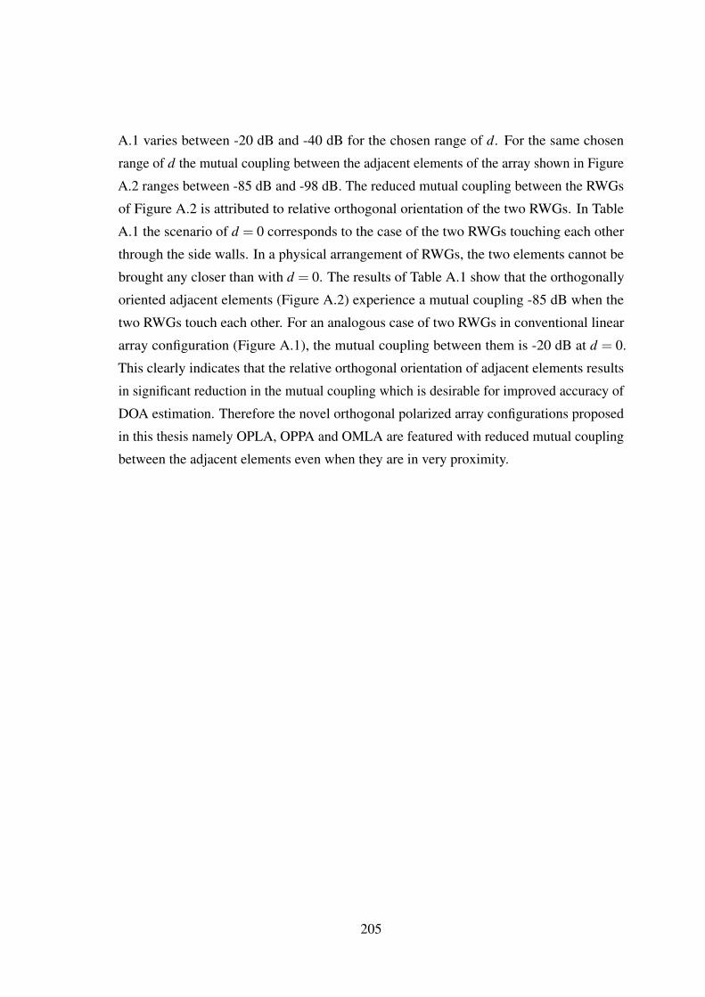
A.1 varies between -20 dB and -40 dB for the chosen range of d. For the same chosen
range of d the mutual coupling between the adjacent elements of the array shown in Figure
A.2 ranges between -85 dB and -98 dB. The reduced mutual coupling between the RWGs
of Figure A.2 is attributed to relative orthogonal orientation of the two RWGs. In Table
A.1 the scenario of d = 0 corresponds to the case of the two RWGs touching each other
through the side walls. In a physical arrangement of RWGs, the two elements cannot be
brought any closer than with d = 0. The results of Table A.1 show that the orthogonally
oriented adjacent elements (Figure A.2) experience a mutual coupling -85 dB when the
two RWGs touch each other. For an analogous case of two RWGs in conventional linear
array configuration (Figure A.1), the mutual coupling between them is -20 dB at d = 0.
This clearly indicates that the relative orthogonal orientation of adjacent elements results
in significant reduction in the mutual coupling which is desirable for improved accuracy of
DOA estimation. Therefore the novel orthogonal polarized array configurations proposed
in this thesis namely OPLA, OPPA and OMLA are featured with reduced mutual coupling
between the adjacent elements even when they are in very proximity.
205

APPENDIX B
Results of Estimation of 2D-DOA of Single Wideband Source for
different SNRs
Additional simulation results pertaining to the estimation of 2D-DOA of single wideband
source are presented in this Appendix. The improved accuracy and reliability of the MUSIC
based DOA estimation algorithm using various orthogonally polarized array configurations
are illustrated for varying SNR scenario. All the results presented in this Appendix are
obtained through subband based technique of DOA estimation of single wideband source.
In particular, only low band signal component of the subband technique is considered in
the simulation results presented in this Appendix.
206

B.1 Estimation of 2D-DOA of Single Wideband Source With Conventional SinglePolarized UPA
Figure B.1: 2D DOA Estimation of Single Wideband Source with UPA for the Signal Model
θ = 15◦ and φ = 30◦ for 10 dB SNR
Figure B.2: 2D DOA Estimation of Single Wideband Source with UPA for the Signal Model
θ = 15◦ and φ = 30◦ for 10 dB SNR - 2D View of Simulation Result
207

Figure B.3: 2D DOA Estimation of Single Wideband Source with UPA for the Signal Model
θ = 15◦ and φ = 30◦ for 20 dB SNR
Figure B.4: 2D DOA Estimation of Single Wideband Source with UPA for the Signal Model
θ = 15◦ and φ = 30◦ for 20 dB SNR - 2D View of Simulation Result
208
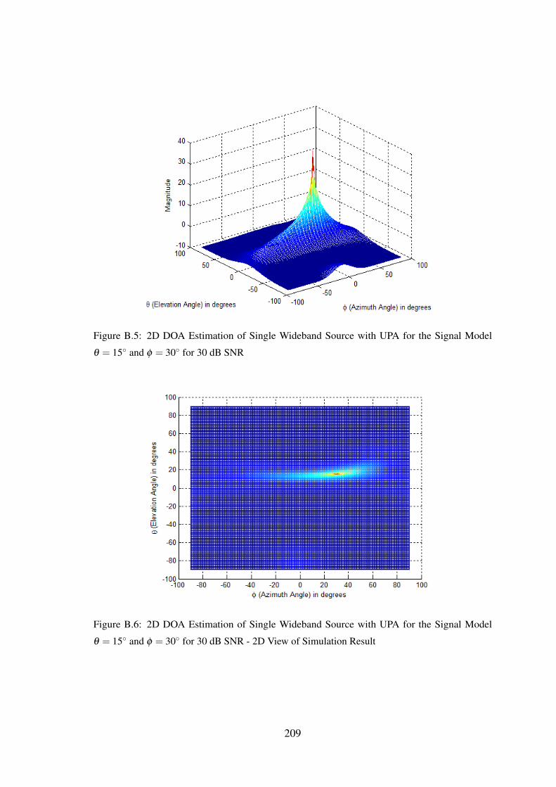
Figure B.5: 2D DOA Estimation of Single Wideband Source with UPA for the Signal Model
θ = 15◦ and φ = 30◦ for 30 dB SNR
Figure B.6: 2D DOA Estimation of Single Wideband Source with UPA for the Signal Model
θ = 15◦ and φ = 30◦ for 30 dB SNR - 2D View of Simulation Result
209

B.2 Estimation of 2D-DOA of Single Wideband Source With OPPA
Figure B.7: 2D DOA Estimation of Single Wideband Source with OPPA for the Signal Model
θ = 15◦ and φ = 30◦ for 10 dB SNR
Figure B.8: 2D DOA Estimation of Single Wideband Source with OPPA for the Signal Model
θ = 15◦ and φ = 30◦ for 10 dB SNR - 2D View of Simulation Result
210

Figure B.9: 2D DOA Estimation of Single Wideband Source with OPPA for the Signal Model
θ = 15◦ and φ = 30◦ for 20 dB SNR
Figure B.10: 2D DOA Estimation of Single Wideband Source with OPPA for the Signal Model
θ = 15◦ and φ = 30◦ for 20 dB SNR - 2D View of Simulation Result
211

Figure B.11: 2D DOA Estimation of Single Wideband Source with OPPA for the Signal Model
θ = 15◦ and φ = 30◦ for 30 dB SNR
Figure B.12: 2D DOA Estimation of Single Wideband Source with OPPA for the Signal Model
θ = 15◦ and φ = 30◦ for 30 dB SNR - 2D View of Simulation Result
212

B.3 Estimation of 2D-DOA of Single Wideband Source With OMLA
Figure B.13: 2D DOA Estimation of Single Wideband Source with OMLA for the Signal Model
θ = 15◦ and φ = 30◦ for 10 dB SNR
Figure B.14: 2D DOA Estimation of Single Wideband Source with OMLA for the Signal Model
θ = 15◦ and φ = 30◦ for 10 dB SNR - 2D View of Simulation Result
213

Figure B.15: 2D DOA Estimation of Single Wideband Source with OMLA for the Signal Model
θ = 15◦ and φ = 30◦ for 20 dB SNR
Figure B.16: 2D DOA Estimation of Single Wideband Source with OMLA for the Signal Model
θ = 15◦ and φ = 30◦ for 20 dB SNR - 2D View of Simulation Result
214
Figure B.17: 2D DOA Estimation of Single Wideband Source with OMLA for Signal Model
θ = 15◦ and φ = 30◦ for 30 dB SNR
Figure B.18: 2D DOA Estimation of Single Wideband Source with OMLA for the Signal Model
θ = 15◦ and φ = 30◦ for 30 dB SNR - 2D View of Simulation Result
215

B.4 Estimation of 2D-DOA of Single Wideband Source With OPLA
Figure B.19: 2D DOA Estimation of Single Wideband Source with OPLA for the Signal Model
θ = 15◦ and φ = 30◦ for 10 dB SNR
Figure B.20: 2D DOA Estimation of Single Wideband Source with OPLA for the Signal Model
θ = 15◦ and φ = 30◦ for 10 dB SNR - 2D View of Simulation Result
216
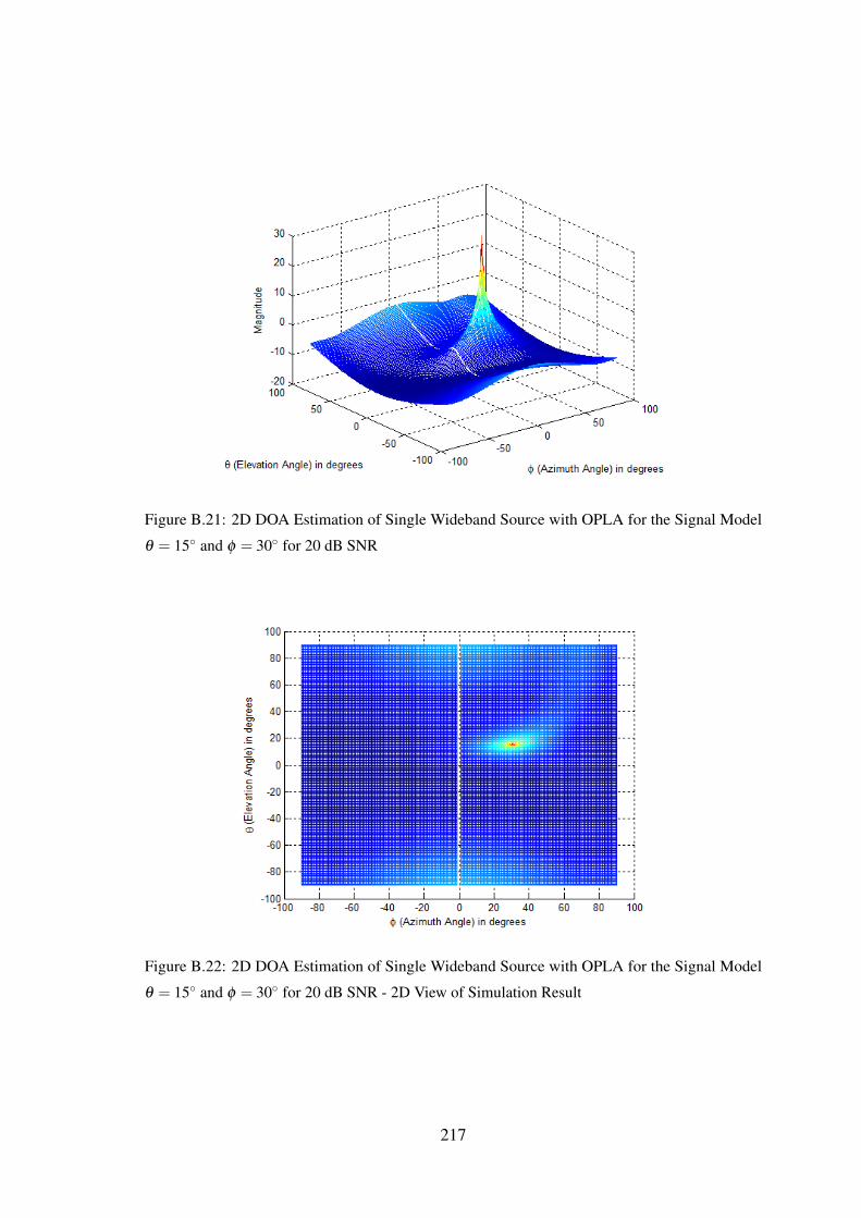
Figure B.21: 2D DOA Estimation of Single Wideband Source with OPLA for the Signal Model
θ = 15◦ and φ = 30◦ for 20 dB SNR
Figure B.22: 2D DOA Estimation of Single Wideband Source with OPLA for the Signal Model
θ = 15◦ and φ = 30◦ for 20 dB SNR - 2D View of Simulation Result
217

Figure B.23: 2D DOA Estimation of Single Wideband Source with OPLA for the Signal Model
θ = 15◦ and φ = 30◦ for 30 dB SNR
Figure B.24: 2D DOA Estimation of Single Wideband Source with OPLA for the Signal Model
θ = 15◦ and φ = 30◦ for 30 dB SNR - 2D View of Simulation Result
218
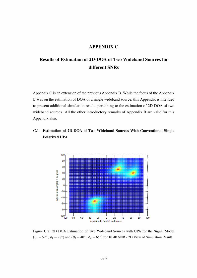
APPENDIX C
Results of Estimation of 2D-DOA of Two Wideband Sources for
different SNRs
Appendix C is an extension of the previous Appendix B. While the focus of the Appendix
B was on the estimation of DOA of a single wideband source, this Appendix is intended
to present additional simulation results pertaining to the estimation of 2D-DOA of two
wideband sources. All the other introductory remarks of Appendix B are valid for this
Appendix also.
C.1 Estimation of 2D-DOA of Two Wideband Sources With Conventional SinglePolarized UPA
Figure C.2: 2D DOA Estimation of Two Wideband Sources with UPA for the Signal Model
(θ1 = 52◦ , φ1 = 28◦) and (θ2 = 40◦ , φ2 = 65◦) for 10 dB SNR - 2D View of Simulation Result
219

Figure C.3: 2D DOA Estimation of Two Wideband Sources with UPA for the Signal Model
(θ1 = 52◦ , φ1 = 28◦) and (θ2 = 40◦ , φ2 = 65◦) for 20 dB SNR
Figure C.4: 2D DOA Estimation of Two Wideband Sources with UPA for the Signal Model
(θ1 = 52◦ , φ1 = 28◦) and (θ2 = 40◦ , φ2 = 65◦) for 20 dB SNR - 2D View of Simulation Result
220
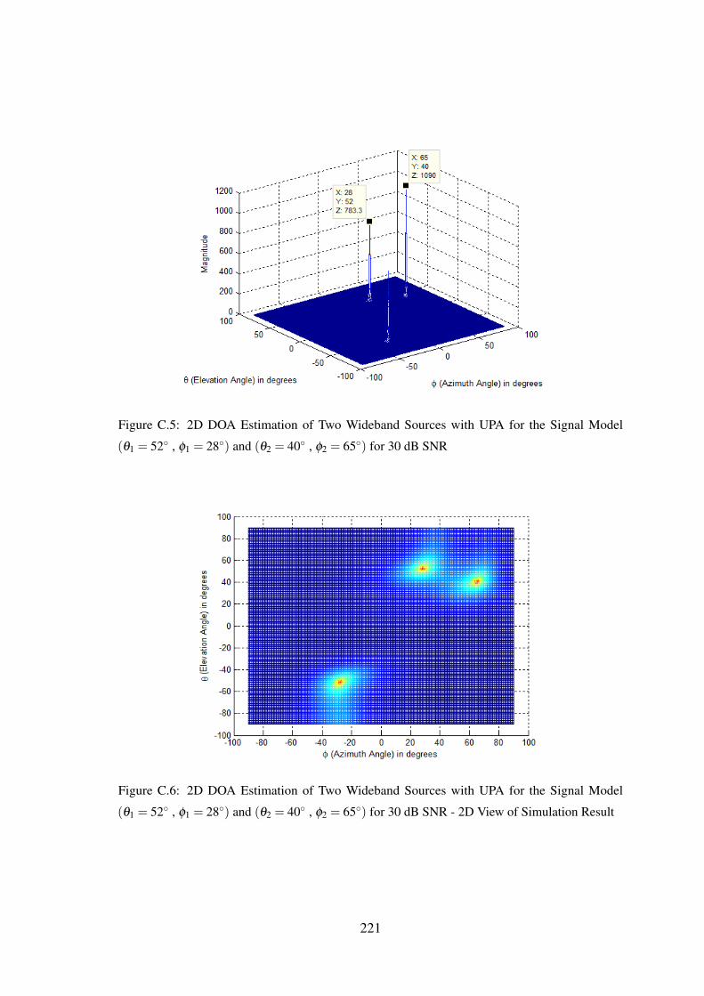
Figure C.5: 2D DOA Estimation of Two Wideband Sources with UPA for the Signal Model
(θ1 = 52◦ , φ1 = 28◦) and (θ2 = 40◦ , φ2 = 65◦) for 30 dB SNR
Figure C.6: 2D DOA Estimation of Two Wideband Sources with UPA for the Signal Model
(θ1 = 52◦ , φ1 = 28◦) and (θ2 = 40◦ , φ2 = 65◦) for 30 dB SNR - 2D View of Simulation Result
221

Figure C.1: 2D DOA Estimation of Two Wideband Sources with UPA for the Signal Model(θ1 = 52◦ , φ1 = 28◦) and (θ2 = 40◦ , φ2 = 65◦) for 10 dB SNR
222

C.2 Estimation of 2D-DOA of Two Wideband Sources With OPPA
Figure C.7: 2D DOA Estimation of Two Wideband Sources with OPPA for the Signal Model
(θ1 = 52◦ , φ1 = 28◦) and (θ2 = 40◦ , φ2 = 65◦) for 10 dB SNR
Figure C.8: 2D DOA Estimation of Two Wideband Sources with OPPA for the Signal Model
(θ1 = 52◦ , φ1 = 28◦) and (θ2 = 40◦ , φ2 = 65◦) for 10 dB SNR - 2D View of Simulation Result
223

Figure C.9: 2D DOA Estimation of Two Wideband Sources with OPPA for the Signal Model
(θ1 = 52◦ , φ1 = 28◦) and (θ2 = 40◦ , φ2 = 65◦) for 20 dB SNR
Figure C.10: 2D DOA Estimation of Two Wideband Sources with OPPA for the Signal Model
(θ1 = 52◦ , φ1 = 28◦) and (θ2 = 40◦ , φ2 = 65◦) for 20 dB SNR - 2D View of Simulation Result
224
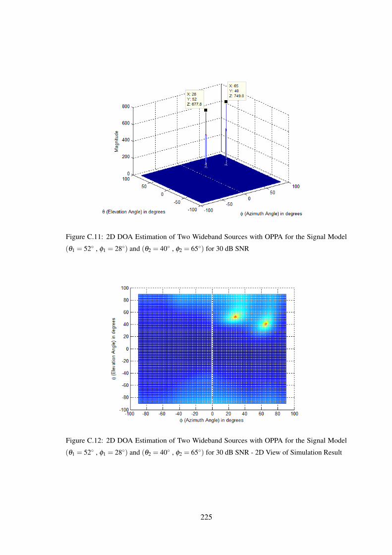
Figure C.11: 2D DOA Estimation of Two Wideband Sources with OPPA for the Signal Model
(θ1 = 52◦ , φ1 = 28◦) and (θ2 = 40◦ , φ2 = 65◦) for 30 dB SNR
Figure C.12: 2D DOA Estimation of Two Wideband Sources with OPPA for the Signal Model
(θ1 = 52◦ , φ1 = 28◦) and (θ2 = 40◦ , φ2 = 65◦) for 30 dB SNR - 2D View of Simulation Result
225
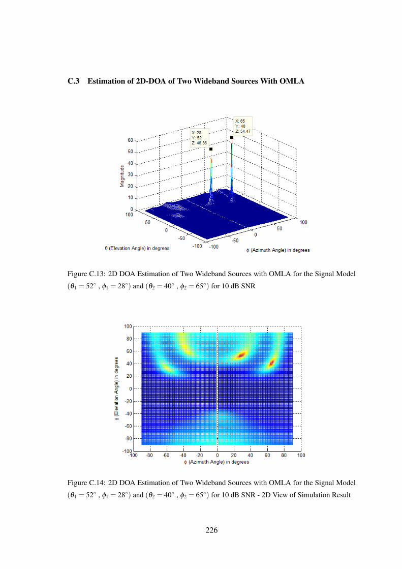
C.3 Estimation of 2D-DOA of Two Wideband Sources With OMLA
Figure C.13: 2D DOA Estimation of Two Wideband Sources with OMLA for the Signal Model
(θ1 = 52◦ , φ1 = 28◦) and (θ2 = 40◦ , φ2 = 65◦) for 10 dB SNR
Figure C.14: 2D DOA Estimation of Two Wideband Sources with OMLA for the Signal Model
(θ1 = 52◦ , φ1 = 28◦) and (θ2 = 40◦ , φ2 = 65◦) for 10 dB SNR - 2D View of Simulation Result
226
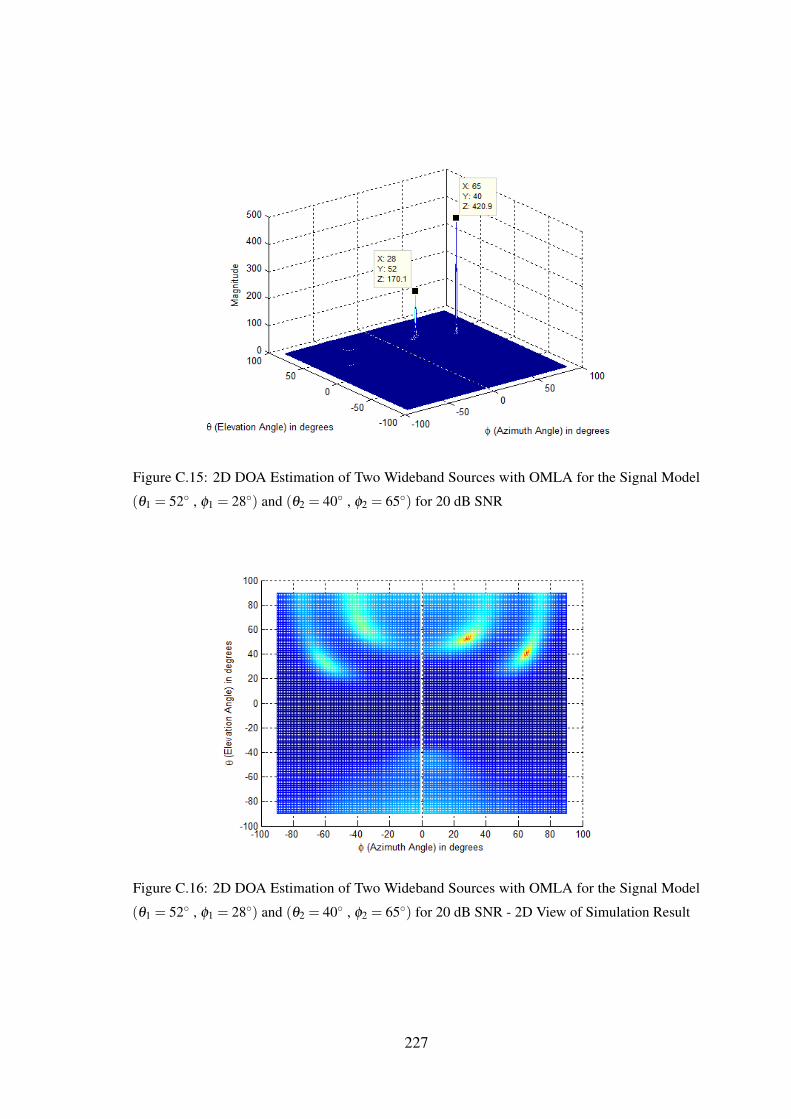
Figure C.15: 2D DOA Estimation of Two Wideband Sources with OMLA for the Signal Model
(θ1 = 52◦ , φ1 = 28◦) and (θ2 = 40◦ , φ2 = 65◦) for 20 dB SNR
Figure C.16: 2D DOA Estimation of Two Wideband Sources with OMLA for the Signal Model
(θ1 = 52◦ , φ1 = 28◦) and (θ2 = 40◦ , φ2 = 65◦) for 20 dB SNR - 2D View of Simulation Result
227
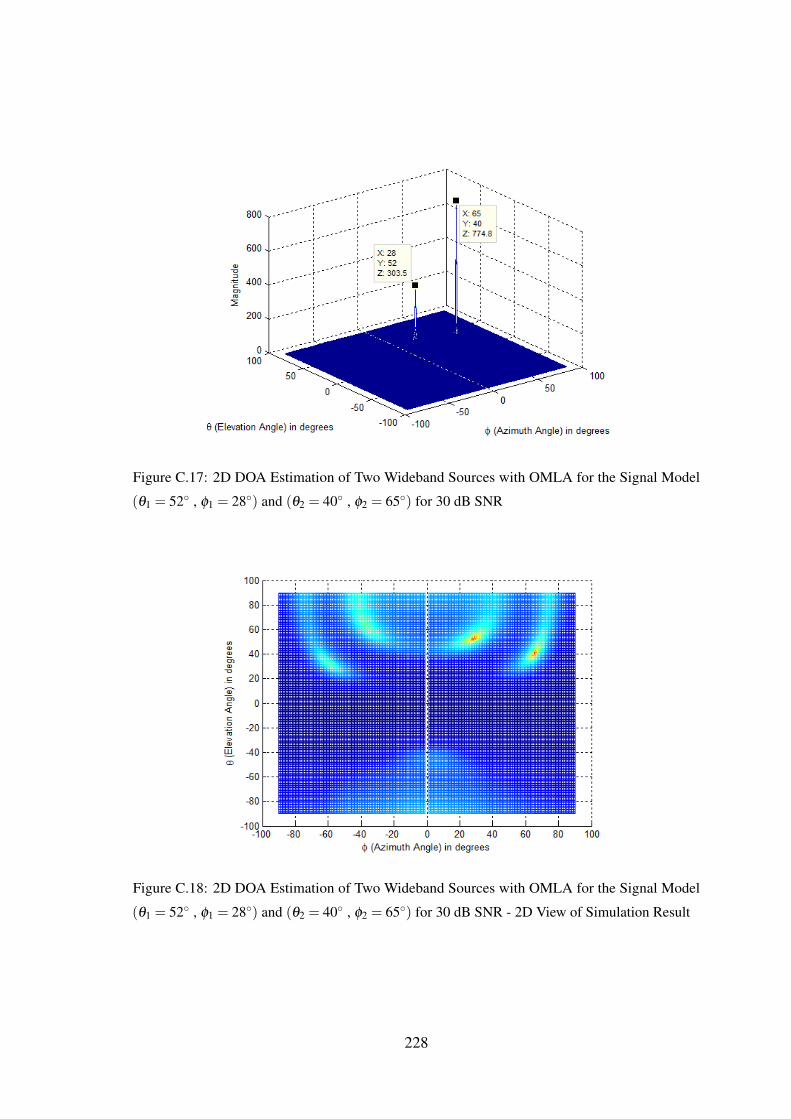
Figure C.17: 2D DOA Estimation of Two Wideband Sources with OMLA for the Signal Model
(θ1 = 52◦ , φ1 = 28◦) and (θ2 = 40◦ , φ2 = 65◦) for 30 dB SNR
Figure C.18: 2D DOA Estimation of Two Wideband Sources with OMLA for the Signal Model
(θ1 = 52◦ , φ1 = 28◦) and (θ2 = 40◦ , φ2 = 65◦) for 30 dB SNR - 2D View of Simulation Result
228
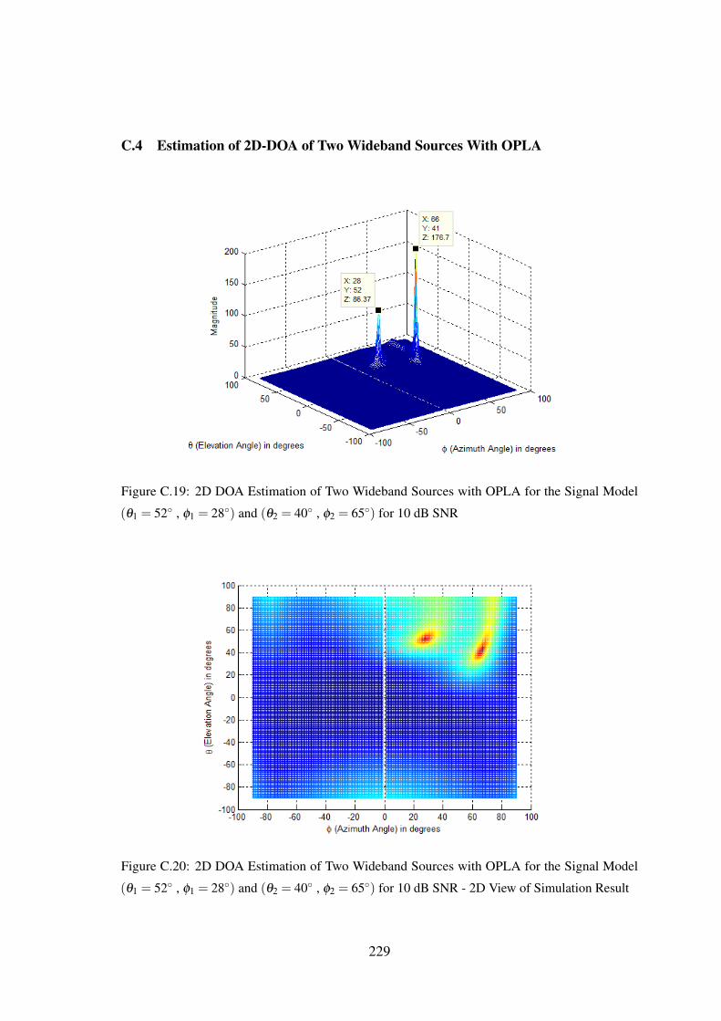
C.4 Estimation of 2D-DOA of Two Wideband Sources With OPLA
Figure C.19: 2D DOA Estimation of Two Wideband Sources with OPLA for the Signal Model
(θ1 = 52◦ , φ1 = 28◦) and (θ2 = 40◦ , φ2 = 65◦) for 10 dB SNR
Figure C.20: 2D DOA Estimation of Two Wideband Sources with OPLA for the Signal Model
(θ1 = 52◦ , φ1 = 28◦) and (θ2 = 40◦ , φ2 = 65◦) for 10 dB SNR - 2D View of Simulation Result
229

Figure C.21: 2D DOA Estimation of Two Wideband Sources with OPLA for the Signal Model
(θ1 = 52◦ , φ1 = 28◦) and (θ2 = 40◦ , φ2 = 65◦) for 20 dB SNR
Figure C.22: 2D DOA Estimation of Two Wideband Sources with OPLA for the Signal Model
(θ1 = 52◦ , φ1 = 28◦) and (θ2 = 40◦ , φ2 = 65◦) for 20 dB SNR - 2D View of Simulation Result
230

Figure C.23: 2D DOA Estimation of Two Wideband Sources with OPLA for the Signal Model
(θ1 = 52◦ , φ1 = 28◦) and (θ2 = 40◦ , φ2 = 65◦) for 30 dB SNR
Figure C.24: 2D DOA Estimation of Two Wideband Sources with OPLA for the Signal Model
(θ1 = 52◦ , φ1 = 28◦) and (θ2 = 40◦ , φ2 = 65◦) for 30 dB SNR - 2D View of Simulation Result
231

APPENDIX D
Low Risk Research Ethics Approval Checklist
232


References
Abed-Meraim, K., Chkeif, A., & Hua, Y. (2000). Fast orthonormal past algorithm. Signal
Processing Letters, IEEE, 7(3), 60–62.
Allen, B., & Ghavami, M. (2006). Adaptive array systems: fundamentals and applications.
John Wiley & Sons.
Balanis, C. A. (2011). Modern antenna handbook. John Wiley & Sons.
Balanis, C. A. (2012). Antenna theory: analysis and design. John Wiley & Sons.
Bartlett, M. S. (1950). Periodogram analysis and continuous spectra. Biometrika, 1–16.
Bunch, J. R., Nielsen, C. P., & Sorensen, D. C. (1978). Rank-one modification of the
symmetric eigenproblem. Numerische Mathematik, 31(1), 31–48.
Capon, J. (1969). High-resolution frequency-wavenumber spectrum analysis. Proceedings
of the IEEE, 57(8), 1408–1418.
Champagne, B. (1994). Adaptive eigendecomposition of data covariance matrices based
on first-order perturbations. Signal Processing, IEEE Transactions on, 42(10),
2758–2770.
Chandran, S. (2005). Advances in direction-of-arrival estimation. Artech House.
Chen, J. C., Yao, K., & Hudson, R. E. (2002). Source localization and beamforming.
Signal Processing Magazine, IEEE, 19(2), 30–39.
Chen, S.-W., Jen, C.-W., & Chang, A.-C. (2009). High-resolution doa estimation based on
independent noise component for correlated signal sources. Neural Computing and
Applications, 18(4), 381–385.
Chick, D. F., Collins, P., Goodman, S., Martin, R., & Terzuoli Jr, A. (2011). Direction
finding with mutually orthogonal antennas. In Antennas and propagation (apsursi),
2011 ieee international symposium on (pp. 2853–2856).
Choudhury, R. R., & Vaidya, N. H. (2003). Impact of directional antennas on ad hoc
routing. In Personal wireless communications (pp. 590–600).
Chryssomallis, M. (2000). Smart antennas. Antennas and Propagation Magazine, IEEE,
42(3), 129–136.
Coldrey, M., & Viberg, M. (2006). Generalization and analysis of the conventional
237
beamformer for localization of spatially distributed sources. In In proc. 14th european
signal processing conference, eusipco 2006.
Comon, P., & Golub, G. H. (1990). Tracking a few extreme singular values and vectors in
signal processing. Proceedings of the IEEE, 78(8), 1327–1343.
Di Claudio, E. D., & Parisi, R. (2001). Waves: weighted average of signal subspaces for
robust wideband direction finding. Signal Processing, IEEE Transactions on, 49(10),
2179–2191.
Doran, M., Doron, M., Weiss, A. J., et al. (1993). Coherent wide-band processing for
arbitrary array geometry. Signal Processing, IEEE Transactions on, 41(1), 414.
Doron, M. A., & Weiss, A. J. (1992). On focusing matrices for wide-band array processing.
Signal Processing, IEEE Transactions on, 40(6), 1295–1302.
Feng, D., Bao, M., Ye, Z., Guan, L., & Li, X. (2011). A novel wideband doa estimator
based on khatri–rao subspace approach. Signal Processing, 91(10), 2415–2419.
Fuhl, J., Rossi, J.-P., & Bonek, E. (1997). High-resolution 3-d direction-of-arrival
determination for urban mobile radio. Antennas and Propagation, IEEE Transactions
on, 45(4), 672–682.
Golub, G. H. (1973). Some modified matrix eigenvalue problems. Siam Review, 15(2),
318–334.
Golub, G. H., & Van Loan, C. F. (2012). Matrix computations (Vol. 3). JHU Press.
Gu, J.-F., Zhu, W.-P., & Swamy, M. (2015). Joint 2-d doa estimation via sparse l-shaped
array. Signal Processing, IEEE Transactions on, 63(5), 1171–1182.
Hansen, R. C. (2009). Phased array antennas (Vol. 213). John Wiley & Sons.
Harabi, F., Changuel, H., & Gharsallah, A. (2007). Direction of arrival estimation method
using a 2-l shape arrays antenna. Progress In Electromagnetics Research, 69, 145–
160.
Hayes, M. H. (2009). Statistical digital signal processing and modeling. John Wiley &
Sons.
Haykin, S. (2008). Communication systems. John Wiley & Sons.
Haykin, S. S. (2008). Adaptive filter theory. Pearson Education India.
He, Z.-Q., Shi, Z.-P., Huang, L., & So, H. C. (2015). Underdetermined doa estimation for
wideband signals using robust sparse covariance fitting. Signal Processing Letters,
IEEE, 22(4), 435–439.
Hu, W., Zhang, A., & Wang, C. (2014). 2d direction of arrival estimation for cross array in
the presence of mutual coupling. International Journal of Antennas and Propagation,
238
2014.
Inoue, Y., Mori, K., & Arai, H. (2002). Doa estimation in consideration of the array
element pattern. In Vehicular technology conference, 2002. vtc spring 2002. ieee
55th (Vol. 2, pp. 745–748).
Karasalo, I. (1986). Estimating the covariance matrix by signal subspace averaging.
Acoustics, Speech and Signal Processing, IEEE Transactions on, 34(1), 8–12.
Karthikeyan, B. R., Kadambi, G. R., & Vershinin, Y. A. (2015). A formulation of 1-d
search technique for 2-d doa estimation using orthogonally polarized components of
linear array. IEEE Antennas and Wireless Propagation Letters, 14.
Kim, J.-T., Kim, S.-t., & Lee, K.-w. (2013). 1 ambiguity analysis method for the calibrated
array manifold.
Kim, M., Takeuchi, T., & Chong, N. Y. (2004). A 3-axis orthogonal antenna for indoor
localization. In First international workshop on networked sensing systems (pp.
59–62).
Kolar, V. (2004). Challenges in directional antennas (Unpublished master’s thesis). State
University of New York.
Kraus, J. (1992). Electromagnetics. McGraw-Hill.
Krim, H., & Viberg, M. (1996). Two decades of array signal processing research: the
parametric approach. Signal Processing Magazine, IEEE, 13(4), 67–94.
Lathi, B. P. (1998). Modern digital and analog communication systems 3e osece. Oxford
university press.
Li, J. (1993). Direction and polarization estimation using arrays with small loops and short
dipoles. Antennas and Propagation, IEEE Transactions on, 41(3), 379–387.
Liang, J., & Liu, D. (2011). Two l-shaped array-based 2-d doas estimation in the presence
of mutual coupling. Progress In Electromagnetics Research, 112, 273–298.
Liao, B., Zhang, Z.-G., & Chan, S.-C. (2012). Doa estimation and tracking of ulas with
mutual coupling. Aerospace and Electronic Systems, IEEE Transactions on, 48(1),
891–905.
Manikas, A., Alexiou, A., & Karimi, H. (1997). Comparison of the ultimate direction-
finding capabilities of a number of planar array geometries. In Radar, sonar and
navigation, iee proceedings- (Vol. 144, pp. 321–329).
Marcos, S., Marsal, A., & Benidir, M. (1995). The propagator method for source bearing
estimation. Signal Processing, 42(2), 121–138.
Nadler, B. (2010). Nonparametric detection of signals by information theoretic criteria: per-
239
formance analysis and an improved estimator. Signal Processing, IEEE Transactions
on, 58(5), 2746–2756.
Ouyang, S., & Hua, Y. (2005). Bi-iterative least-square method for subspace tracking.
Signal Processing, IEEE Transactions on, 53(8), 2984–2996.
Owsley, N. L. (1978). Adaptive data orthogonalization. In Acoustics, speech, and signal
processing, ieee international conference on icassp’78. (Vol. 3, pp. 109–112).
Pisarenko, V. F. (1973). The retrieval of harmonics from a covariance function. Geophysical
Journal International, 33(3), 347–366.
Rajagopalan, J. (1996). An iterative algorithm for inversion of matrices (Unpublished
doctoral dissertation). Concordia University.
Rappaport, T. S., Reed, J., & Woerner, B. D. (1996). Position location using wireless
communications on highways of the future. Communications Magazine, IEEE,
34(10), 33–41.
Roy, R., & Kailath, T. (1989). Esprit-estimation of signal parameters via rotational
invariance techniques. Acoustics, Speech and Signal Processing, IEEE Transactions
on, 37(7), 984–995.
Schmidt, R. O. (1986). Multiple emitter location and signal parameter estimation. Antennas
and Propagation, IEEE Transactions on, 34(3), 276–280.
Schreiber, R. (1986). Implementation of adaptive array algorithms. IEEE transactions on
acoustics, speech, and signal processing, 34, 1038–1045.
Sellone, F. (2005). Robust wideband doa estimation. In Statistical signal processing, 2005
ieee/sp 13th workshop on (pp. 277–282).
Sellone, F. (2006). Robust auto-focusing wideband doa estimation. Signal Processing,
86(1), 17–37.
Shaghaghi, M., & Vorobyov, S. (2015). Subspace leakage analysis and improved doa
estimation with small sample size.
Shan, T.-J., Wax, M., & Kailath, T. (1985). On spatial smoothing for direction-of-arrival
estimation of coherent signals. IEEE Transactions on Acoustics, Speech, and Signal
Processing, 33(4), 806–811.
Silver, S. (1949). Microwave antenna theory and design (No. 19). Iet.
Stoica, P., & Moses, R. L. (1997). Introduction to spectral analysis (Vol. 1). Prentice hall
Upper Saddle River, NJ.
Stoica, P., & Soderstrom, T. (1991). Statistical analysis of music and esprit estimates of
sinusoidal frequencies. In Acoustics, speech, and signal processing, 1991. icassp-91.,
240
1991 international conference on (pp. 3273–3276).
Stoica, P., & Soderstrom, T. (1991). Statistical analysis of music and subspace rotation
estimates of sinusoidal frequencies. Signal Processing, IEEE Transactions on, 39(8),
1836–1847.
Strobach, P. (1997). Bi-iteration svd subspace tracking algorithms. Signal Processing,
IEEE Transactions on, 45(5), 1222–1240.
Tayem, N., & Kwon, H. M. (2005). L-shape 2-dimensional arrival angle estimation
with propagator method. Antennas and Propagation, IEEE Transactions on, 53(5),
1622–1630.
Tayem, N. A.-H. M. (2005). Direction of arrival angle estimation schemes for wire-
less communication systems (Unpublished doctoral dissertation). Wichita State
University.
IEEE standard definitions of terms for antennas. (1983, June). IEEE Std 145-1983, 1-31.
doi: 10.1109/IEEESTD.1983.82386
Tuncer, T. E., & Friedlander, B. (2009). Classical and modern direction-of-arrival
estimation. Academic Press.
Vaidyanathan, P. P. (1993). Multirate systems and filter banks. Pearson Education India.
Van Trees, H. L. (2004). Detection, estimation, and modulation theory, optimum array
processing. John Wiley & Sons.
Van Veen, B. D., & Buckley, K. M. (1988). Beamforming: A versatile approach to spatial
filtering. IEEE assp magazine, 5(2), 4–24.
Vershinin, Y. A. (2014). Adaptive control system for solution of fault tolerance problem.
In Iaeng transactions on engineering technologies (pp. 197–207). Springer.
Visser, H. J. (2006). Array and phased array antenna basics. John Wiley & Sons.
Wang, H., & Kaveh, M. (1985). Coherent signal-subspace processing for the detection and
estimation of angles of arrival of multiple wide-band sources. Acoustics, Speech and
Signal Processing, IEEE Transactions on, 33(4), 823–831.
Wax, M. (1989). Detection of the number of coherent signals by the mdl principle. IEEE
Trans. Acoust., Speech, Signal Processing, 37(8), 1190–1196.
Wax, M., & Kailath, T. (1985). Detection of signals by information theoretic criteria.
Acoustics, Speech and Signal Processing, IEEE Transactions on, 33(2), 387–392.
Wei, Y., & Guo, X. (2014). Pair-matching method by signal covariance matrices for 2d-doa
estimation. Antennas and Wireless Propagation Letters, IEEE, 13, 1199–1202.
Weiss, A. J., & Friedlander, B. (1993). Direction finding for diversely polarized signals
241

using polynomial rooting. Signal Processing, IEEE Transactions on, 41(5), 1893–
1905.
Wong, K. T., Li, L., & Zoltowski, M. D. (2004). Root-music-based direction-finding and
polarization estimation using diversely polarized possibly collocated antennas. IEEE
Antennas and Wireless Propagation Letters, 3(1), 129–132.
Wong, K. T., & Zoltowski, M. D. (1998). Closed-form direction-finding with arbitrarily
spaced electromagnetic vector-sensors at unknown locations. In Acoustics, speech
and signal processing, 1998. proceedings of the 1998 ieee international conference
on (Vol. 4, pp. 1949–1952).
Woods, J. W., & O’Neil, S. D. (1986). Subband coding of images. Acoustics, Speech and
Signal Processing, IEEE Transactions on, 34(5), 1278–1288.
Wu, Y., Liao, G., & So, H.-C. (2003). A fast algorithm for 2-d direction-of-arrival
estimation. Signal processing, 83(8), 1827–1831.
Yang, B. (1995). Projection approximation subspace tracking. Signal Processing, IEEE
Transactions on, 43(1), 95–107.
Yang, J.-F., & Kaveh, M. (1988). Adaptive eigensubspace algorithms for direction or
frequency estimation and tracking. Acoustics, Speech and Signal Processing, IEEE
Transactions on, 36(2), 241–251.
Yilmazer, N., Koh, J., & Sarkar, T. K. (2006). Utilization of a unitary transform for
efficient computation in the matrix pencil method to find the direction of arrival.
Antennas and Propagation, IEEE Transactions on, 54(1), 175–181.
Yoon, Y.-S. (2004). Direction-of-arrival estimation of wideband sources using sensor
arrays (Unpublished doctoral dissertation). Georgia Institute of Technology.
Yoon, Y.-S., Kaplan, L. M., & McClellan, J. H. (2006). Tops: new doa estimator for
wideband signals. Signal Processing, IEEE Transactions on, 54(6), 1977–1989.
Yoshimura, S., Ushijima, Y., Nishiyama, E., & Aikawa, M. (2011). Microstrip array
antenna for orthogonal linear polarization discrimination. In Proc. international
symposium on antenna and propagation, wed1-2.
Yu, H., Liu, J., Huang, Z., Zhou, Y., & Xu, X. (2007). A new method for wideband doa
estimation. In Wireless communications, networking and mobile computing, 2007.
wicom 2007. international conference on (pp. 598–601).
Zhang, J., Dai, J., & Ye, Z. (2010). An extended tops algorithm based on incoherent signal
subspace method. Signal Processing, 90(12), 3317–3324.
242