development of robotics simulation using creo 2

1 Copyright © 2014 by ASME

DEVELOPMENT OF ROBOTICS SIMULATION USING CREO 2.0

Shubham Somani Student [email protected]

Anshul Jain Student [email protected]

Vimal Savsani Assistant Professor [email protected]

Poonam Savsani Assistant Professor [email protected]

Department of Mechanical Engineering Pandit Deendayal Petroleum University

Gandhinagar, Gujarat, India

ABSTRACT Simulation of robot systems is getting very popular,

especially with the lowering cost of computers. The robotic arm

is presumably the most mathematically complex for the

dynamic and kinematic analysis. The purpose of this paper is to

build a simulation framework for a 3R robotic arm using PTC

Creo Parametric 2.0 and also to identify its advantages and

disadvantages for such analysis. Trajectory of the robotic arm is

optimized by considering the shortest path as an objective

function between the initial and final position which results in

straight line motion using an effective optimization technique

known as Teaching learning based optimization (TLBO).

Intermediate positions of the optimized results are taken as an

input for the simulation of the 3R robotic arm in PTC Creo

Parametric 2.0.The results obtained by using TLBO and PTC

Creo Parametric 2.0, such as angular positions, joint velocities

and joint accelerations are compared based on RMS errors. The

verification of the obtained results by both the methods allows

us to qualitatively evaluate, underline the rightness of the

chosen model and to get the right conclusions.

INTRODUCTION

Simulation is the method for emulating and predicting the

behavior and the operation of a robotic system based on the

model of the physical system [1]. Simulation provides core

simulation tools to test designs and make the decisions to

improve quality. The full integration creates a short learning

curve and eliminates the redundant tasks required with

traditional analysis tools. Component materials, connections,

and relationships defined during design development are fully

understood in simulation [2]. Products can be tested for strength

and safety, and also the kinematics can be fully analyzed. The

main aim of this paper is to generate a model for kinematic

analysis of a 3R robotic arm using PTC Creo Parametric 2.0

and also to identify its advantages and disadvantages. PTC Creo

Parametric 2.0 provides the broadest range of powerful yet

flexible 3D CAD capabilities to help in most pressing design

challenges including accommodating late stage changes,

working with multi-CAD data, intuitive 3D design, create 2D

drawings faster, test real world conditions etc [3]. In a

kinematic analysis the position, velocity and acceleration of all

the links are calculated without considering the forces that

cause this motion. The kinematics separate in two types,

forward kinematics and inverse kinematics. Both forward

kinematics and inverse kinematics are used in this paper for the

path planning of a 3R robotic arm [4,5] . The path planning is

the planning of the whole path which refers to the complete

route traced from the start to the goal end point. The path is

made up of a number of segments and each of these path

segments is continuous and is called trajectory. This is

significant, when considering a trajectory planner, which

basically chooses a locally optimal direction, as opposed to a

complete path [6]. Tasks of robot control can be classified in

different ways. For example, different path planning strategies

can be used in the case of different situations. There are two

types of constraints that must be considered in path planning.

First, the motion of a robot can be restricted by obstacles and

obstacle constraints have to be used. On the other hand there

can be some kind of constraints for path selection. These

constraints are known as path constraints [7]. In this simulation,

straight line trajectory is considered as a path constraint. In this

paper, to aid the description of the path planning problem, a

generalized statement of the optimization criteria is given. This

is presented for both the measure of performance and

constraints. The first most important measure of performance is

initial and final coordinates of robotic manipulator and to get

the straight line trajectory. To find this and other factors, a

Proceedings of the ASME 2014 International Mechanical Engineering Congress and Exposition IMECE2014

November 14-20, 2014, Montreal, Quebec, Canada

IMECE2014-39545


number of relations will be derived. First assume that the path is

made up of a number of discrete segments (trajectories). These

segments are linked together to form the path of motion.

Straight line motion is defined as the motion along a straight

line or movement of a rigid body along a straight line and

represents the shortest distance between the two points in the

3D workspace of any robot. The straight line motion from the

source to the goal covered is known as the straight line

trajectory [8]. The applications of straight line motion includes

conveyor belt operations, straight line seam arc welding,

inserting peg into a hole, threading a nut onto a bolt, performing

screw transformations, for inserting electronic components onto

PCB etc. In the present world of automation, dependency on

robotics has significantly increased and hence the development

in this field also. Various software, specialized for robotics are

available for specific and specialized purpose such as Webot,

RoKiSim, EyeSim, Robotics Simulator, RoboLogix etc. Apart

from having these specialized software for robotics, PTC Creo

Parametric 2.0 is used in this paper because it is easily

accessible, user friendly, used in many industries and is

relatively new version of PTC and so far no work has been

reported on simulation of 3-R robotic arm using PTC Creo

Parametric 2.0. In this paper, first the design of 3-R manipulator

system is generated and according to the problem statement, it

is required to follow a straight line to move between desired

coordinates using the inputs obtained from optimization through

TLBO. The procedure is discussed in the section of

methodology.

MATHEMATICAL MODELING AND OPTIMIZATION In this paper, three degree of freedom planar robotic arm

is considered as shown in Figure 3, where, the end effecter is

required to move from starting point to final point in free work

space [9]. For the motion planning of the 3R robotic arm, point-

to-point trajectory is considered which is connected by several

small segments. For the considered problem the complete

trajectory is divided into two parts which results in one

intermediate position in-between initial and final position of the

robotic arm. Initial joint angles are obtained by using inverse

kinematics, which requires coordinates of initial position (xi,yi)

and angle Øe for the end effecter. Initial and final velocity (vip ,

vfp =0, p=1,2,3) and acceleration (aip , afp =0, p=1,2,3) are

assumed to be zero for all the joints. Intermediate position,

velocity and acceleration are considered as the design variables,

which can vary during the optimization process in-between the

lower and the upper limits specified. As initial acceleration is

specified and intermediate acceleration is required to be

obtained, so, fourth order trajectory is used from the initial to

the intermediate position, which only requires initial

acceleration. Trajectory from the intermediate to the final

position will have initial acceleration equals to the final

acceleration of the fourth order trajectory at the intermediate

position to maintain the continuity of the acceleration for the

trajectory. So, trajectory from the intermediate to the final

position will have well defined initial and final acceleration

which requires fifth order trajectory to be used in this section.

The fourth order trajectory to be used from the initial to the

intermediate position is given by Equation (1).

)1(4

4

3

3

2

2101, iiiiiiiiiii tatatataat

Where (ai0,…,ai4) are constants to be determined. The required

positions, velocities and accelerations can be determined as

given in Equations.

0ii a ,

4

4

3

3

2

2101 iiiiiiiiii TaTaTaTaa ,

1

.

ia ,

3

4

2

3211

.

432 iiiiiiii TaTaTaa ,

2

..

2 ia (2)

Where Ti is the execution time from point i (initial position) to

point i+1(intermediate position). The above equation can be

solved for the required constants (ai0,…,ai4) from the given

values of initial position and design variables. After obtaining

values of constants, the intermediate point (i+1)'s acceleration

can be obtained as given in Equation (3).

)3(1262 2

4321

..

iiiiii TaTaa

The fifth order trajectory to be used between intermediate and

final position is given by Equation (4).

)4()( 5

5

4

4

3

3

2

210,1 iiiiiiiiiiifi tbtbtbtbtbbt

Where (bi0,…,bi5) are constants to be determined. The required

positions, velocities and accelerations can be determined as

given in Equation (5).

0ii b, 1

.

ii b

5

5

4

4

3

3

2

2101 iiiiiiiiiiii TbTbTbTbTbb ,

4

5

3

4

2

3211

.

5432 iiiiiiiiii TbTbTbTbb ,

2

..

2 ii b,

)5(201262 3

5

2

4321

..

iiiiiiii TbTbTbb

Equation (5) is required to be solved for the six unknowns from

the given final position and design variables.

For obtaining a straight line trajectory, the robot motion

planning is converted into an optimization problem , which

minimizes the distance between the initial and the final position.

The expression for the minimum Cartesian length is given by

equation 6.


)6(),(,),(2

1

b

j

jjclength yxyxdf

Where, (x,y)j represents the Cartesian coordinates of jth

position and d((x,y)j, (x,y)j-1)) calculates the distance between j

and j-1 positions.

The dynamic equations of the 3R robotic arm are calculated

using Lagrangian-Euler dynamics algorithm [10]. Constraints

are imposed on the problem in the terms of maximum torques

taken by the joints calculated by using Lagrangian-Euler

dynamics algorithm. The three constraints for three joints are

given by Equation (7).

gi(X): Tori≤Torimax, (7)

where, i=1,2,3 represents joint, X represents the design

variables.

Further constraint is imposed on the problem to ensure the

robotic arm to reach the final position. The solution is

considered as infeasible, if the final position is not reached with

the given value of Ø for the end effecter. This results in equality

constraints which is given in Equation (8).

g4(X) :X calculated=Xfinal

g5(X) :Y calculated=Yfinal (8)

The above problem requires 9 design variables given in

Equation (9).

213

.

2

.

1

.

321 ,,,,,,,, TTiiiiii (9)

Where θi1 to i3 represents intermediate joint angles, Ø

represents angle of end effector for the intermediate position,

31

.

toii represents intermediate velocity and T1,2 represents time

from initial to intermediate and from intermediate to final

position respectively. Upper and lower limits for the design

variable are considered such that it can cover whole work

volume generated by the robotic arm and it is given by Equation

(10).

i,3,2,1 , 4/4/ ,3,2,1

.

i ,

81.0 2,1 T,

(10)

The above problem is solved by using an effective optimization

technique known as Teaching-Learning Based Optimization

(TLBO). The TLBO method is based on the effect of the

influence of a teacher on the output of learners in a class

[11,12,13]. Like other nature inspired algorithms, TLBO is also

a population based method which uses a population of solutions

to proceed to the global solution. For TLBO population is

considered as a group of learners or a class of learners. In

optimization algorithms population consists of different design

variables. In TLBO different design variables will be analogous

to different subjects offered to learners and the learners‟ result is

analogous to the „fitness‟ as in other population based

optimization techniques. The teacher is considered as the best

solution obtained so far. The process of working of TLBO is

divided into two parts. The first part consists of „Teacher Phase‟

and the second part consists of „Learner Phase‟. The „Teacher

Phase‟ means learning from the teacher and the „Learner Phase‟

means learning due through the interaction between learners.

Teacher Phase: Update the solution using Equation (11). If the

new solution is better than the existing solution, replace the

existing solution with the new one.

)11(,, iFnewiioldinew MTMrXX

Obtain the value of objective function. If the new solution is

better than the existing solution, replace the existing solution

with the new one.

For i=1:Pn

Randomly choose another learner Xj, such that i≠j

If f(Xi)<f(Xj), Xnew,i=Xold,i+ri(Xi-Xj)

Else, Xnew,i=Xold,i+ri(Xj-Xi)

End

TLBO has gained popularity with its effective applications to

many real life optimization problems like multi-objective

placement of the automatic regulators in the distribution system

[14], data clustering [15], environmental economic problems

[16], optimization of planar steel frames [17], dynamic

economic dispatch problem [18], 3D image registration [19].

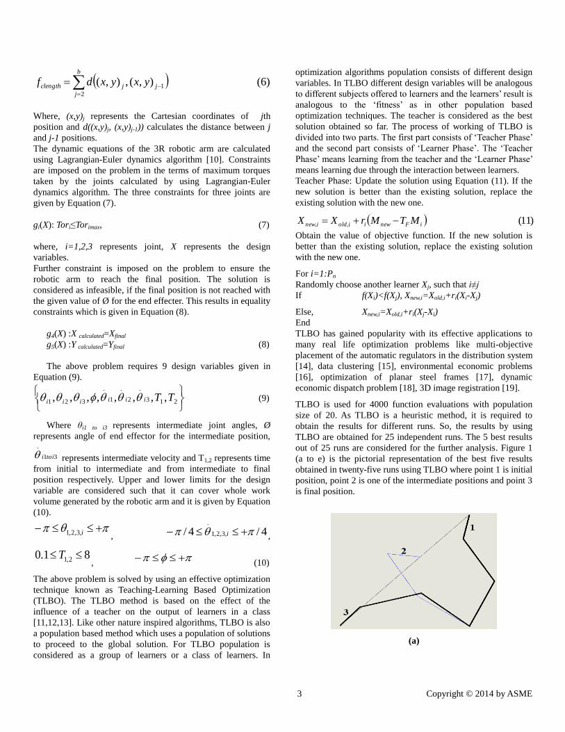
TLBO is used for 4000 function evaluations with population

size of 20. As TLBO is a heuristic method, it is required to

obtain the results for different runs. So, the results by using

TLBO are obtained for 25 independent runs. The 5 best results

out of 25 runs are considered for the further analysis. Figure 1

(a to e) is the pictorial representation of the best five results

obtained in twenty-five runs using TLBO where point 1 is initial

position, point 2 is one of the intermediate positions and point 3

is final position.

(a)


(b)

(c)

(d)

(e)

Figure 1. Five best results obtained using TLBO

a-case1, b-case2, c-case3, d-case4, e-case5

METHODOLOGY The methodology of the whole procedure is shown in

figure 2.

Figure 2. Flow chart of methodology

First, the individual links are generated according to the

problem statement. Volume of the links is found out and

accordingly the material with suitable density to satisfy the mass

property is selected. The base (separately generated) is fixed

and the links are assembled and servo motor is introduced at

each joint by giving different constraints in PTC Creo

Parametric 2.0 as shown in figure 3.

Problem statement (to

obtain straight line)

Generation of 3-D model in

PTC Creo Parametric 2.0

with specified parameters

Optimization of shortest

path between specified

coordinates using TLBO

Data like intermediate position and

intermediate time which are

obtained from TLBO are used as an

input to the generated model to

achieve similar motion.

Kinematic parameters and

coordinated are obtained

Comparison of results

obtained from MATLAB

and that from PTCCreo

Parametric 2.0

Five such sets are obtained

using same steps


Figure 3. Initial position of generated model

The coordinate system is generated taking base as the origin

and selecting axes such that the model‟s motion is in X-Z plane.

Constructing of coordinate system can be done by two ways in

PTC Creo Parametric 2.0. First option is CSYS axes which

enable to rotate the X, Y and Z axes of the new coordinate

system with respect existing coordinate system. The second

option is reference; it enables to select reference geometry for

any two axes of coordinate system. By defining these two axes

will automatically orient the third axis. This model is created

by using the first way. Intermediate angular positions at

corresponding intermediate time are generated from TLBO for

each link of the model. These respective data are used as an

input after suitable conversion in PTC Creo Parametric 2.0 for

each motor in the form of table input. Then interpolated values

are obtained in the form of „spline fit‟ as shown in figure 4.

Figure 4. Parameters in one of the servo motors

After giving input in all the servo motors, kinematic analysis is

done to obtain the motion from initial to final position. Starting

and final time is given in the analysis in such a way that it

satisfies the coordinate constraints as shown figure 5.

Figure 5. Analysis definition of generated model

This analysis results in the motion leading final coordinate as

given in the problem statement as shown in figure 6.

Figure 6. Final position of generated model in one of the cases

Now coordinates of the tip of the model is analyzed throughout

the motion by giving suitable parameters like „Measure v/s

Measure‟ and selecting proper axes in the Measure Results

option as shown in figure 7.


Figure 7. Measurement analysis

Figure 8. X (inch) v/s Z (inch) Coordinates

Now graphs for angular positions, velocity and acceleration

with respect to time are obtained in PTC Creo Parametric 2.0

for each servo motor as shown in figure 9.

Figure 9. Set of graph of angular positions (degree), joint

velocities (degree/sec) and joint acceleration (degree/ sec2)

with respect to time respectively

The results in the form of graphs are exported to excel giving

values of angular positions, velocities and acceleration with

corresponding interpolated time; and coordinates. All these

data, along with data (converted in same units to that of data

from PTC Creo Parametric 2.0) obtained from TLBO are

compared in the graphical form and then the RMS value of

error/difference is found out. Following figures show graphical

comparisons for one of the five sets of results.

Figure 10. Comparision between coordinates of PTC Creo

Parametric 2.0 and TLBO

Figure 11. Position (degree) v/s Time (sec) of one of the links

Figure 12. Velocity (degree/sec) v/s Time (sec) of one the links


Figure 13. Accleration (degree/sec2) v/s Time (sec) of one of

the links

The graphs in figure (11-13) are for one of the three servo

motors. Similar graphs are obtained for all three motors and for

all the five set of values.

In order to judge the accuracy of TLBO to be used as reference

for motion using PTC Creo Parametric 2.0, results of TLBO

(coordinates of tip) are compared with that of ideal motion

(called exact solution) and total distance travelled during

motion of tip is found out for both TLBO and exact solution in

all the five sets and RMS value of error is found out as shown in

Table 1.

Table 1. Comparison of errors

(Here exact/ desired length is 3.07495 and all the errors are absolute errors with respect to length in exact solution)

Table 2. Comparison of errors of PTC Creo Parametric 2.0 and TLBO coordinates with the coordinates of exact solution (Straight-

Line) given points

The results like angular positions, joint velocities, joint

accelerations for each link and coordinate of the tip in all the

five cases in both TLBO and PTC Creo Parametric 2.0 are

obtained and difference in the graphs are compared by finding

out the RMS values of differences/error for all the sets, the

values of which are shown in Table 3.

Table 3. RMS Values of Positions, Velocities and Accelerations


RESULTS AND DISCUSSIONS Ideal total distance required to travel by tip of link is

3.07495 and results from Table 1 show that distance travelled

in results from TLBO has absolute value of variation with

respect to exact solution ranging from 0.023684 to 0.026872.

Also, results from Table 2 show the variation of coordinates

obtained in PTC Creo Parametric 2.0 and TBLO in the terms

of RMS value of the difference. It varies in PTC Creo

Parametric 2.0 from 0.062227 to 0.085634 and that in TBLO

from 0.002827 to 0.029854, indicating variation is very small

and motion is almost straight line. Results of Table 3 shows the

RMS value of errors in PTC Creo Parametric 2.0 with respect

to results obtained in TLBO. Absolute average value of errors

for Positions show that variation is little but for Velocities and

Accelerations show greater variation because only six values

of intermediate time and positions were introduced out of forty

obtained values. But overall result suggests that PTC Creo

Parametric 2.0 is a good method for simulation of 3-R robotic

arm. In spite of having so many advantages like being user

friendly, reliable, having wide applications etc. some of the

limitations are found in PTC Creo Parametric 2.0 while

working like- although the graphs obtained in PTC Creo

Parametric 2.0 can be exported as excel files but tabular input,

directly from the excel cannot be used as Table Input in servo

motor parameter for kinematic analysis. Also upon having

equation of angular displacement as a function of time, it

cannot be used as Polynomial Input in servo motor parameter

as maximum degree of input for polynomial is three. Apart

from that, the reference of angles between two entities (links in

this case) cannot be changed manually; it is taken by PTC

Creo Parametric 2.0 as default. It leads to enormous

calculation while converting in parameters similar to that of

TLBO so that they can be compared.

CONCLUSIONS TLBO is an effective method to obtain a straight line

motion as the RMS value of error between the exact solution

and TLBO is significantly less. Also after observing various

results and comparing TLBO and PTC Creo Parametric 2.0, it

may be concluded that the model generated in PTC Creo

Parametric 2.0 follows almost straight line. There are also

some limitations along with certain possibilities of

improvement as having limitations lead to the focus on further

improvement. Work can be reported in future to have some

generalized mathematical formula/model so as to achieve

desired motion just by giving initial and final coordinates, so

that dependency on another model like TLBO can be

eliminated. The future work will consist of implementing the

proposed methodology for a robotic arm considering tool

orientation and also it can be validated experimentally.

REFERENCES [1] Zha, X.F., Du, H., 2001, “Generation and simulation of

robot trajectories in a virtual CAD-based off-line

programming environment”, The International Journal of

Advanced Manufacturing Technology, 17(8), pp. 610-

624.

[2] Vollmann, K., 2002, “A new approach to robot simulation

tools with parametric components”, IEEE International

Conference on Industrial Technology , 2, pp. 881-885.

[3] http://www.ptc.com/product/creo/parametric

[4] Crane III, C.D., Duffy, J., 2008, “Kinematic analysis of

robot manipulators”, Cambridge University Press.

[5] Yetim, C., 2009, “Kinematic Analysis of Robotic Arm”,

Yildiz Technical University, Istanbul (Turkey), pp. 1-2.

[6] Pfeiffer, F., Johanni, R., 1987, “A concept for

manipulator trajectory planning”, IEEE Journal of

Robotics and Automation, 3(2), pp. 115-123.

[7] Shin, K.G., McKay, N.D., 1986, “Selection of near-

minimum time geometric paths for robotic manipulators”,

IEEE Transactions on Automatic Control, 31(6), pp. 501-

511.

[8] Taylor, R. H., 1979, “Planning and execution of straight

line manipulator trajectories”, IBM Journal of Research

and Development, 23(4), pp. 424-436.

[9] Savsani, P., Jhala, R. L., Savsani, V. J. 2013, “ Optimized

trajectory planning of a robotic arm using teaching

learning based optimization (TLBO) and artificial bee

[10] Craig, J.J., 1989, “Introduction to Robotics: Mechanics and

Control”, 7, Addison-Wesley.

[11] Rao, R.V., Savsani, V.J., Vakharia, D.P., 2011, “Teaching–

learning-based optimization: A novel method for constrained

mechanical design optimization problems. Computer-Aided

Design”, 43(3), pp. 303-315.

[12] Rao, R.V., Savsani, V.J., Vakharia, D.P., 2012, “Teaching–

learning-based optimization: an optimization method for

continuous non-linear large scale problems”, Information

Sciences, 183(1), pp. 1-15.

[13] Rao, R.V., Savsani, V.J., 2012, “Mechanical design

optimization using advanced optimization techniques”,

London Springer.

[14] Hosseinpour, H., Niknam, T., Taheri, S.I., 2011, “A modified

TLBO algorithm for placement of AVRs considering DGs”,

26th International Power System Conference, Tehran, Iran.

[15] Pawar, P.J., Rao, R.V., 2013, “Parameter optimization of

machining processes using teaching–learning-based

optimization algorithm”, The International Journal of

Advanced Manufacturing Technology, 67(5-8), pp. 995-1006.

[16] Ramanand, K.R., Krishnanand, K.R., Panigrahi, B.K.,

Mallick, M.K., 2012, “Brain Storming Incorporated Teaching

colony (ABC) optimization techniques”, IEEE International

Systems Conference, pp. 381-386.


[17] Toğan, V. 2012, “Design of planar steel frames using

teaching–learning based optimization”, Engineering

Structures, 34, pp. 225-232.

[18] Niknam, T., Golestaneh, F., Sadeghi, M.S., 2012,

“Multiobjective Teaching–Learning-Based Optimization for

Dynamic Economic Emission Dispatch”, IEEE Systems

Journal, 6(2), pp. 341-352.

[19] Jani, A., Savsani, V.J., Pandya, A., 2013, “3D affine

registration using teaching-learning based optimization”, 3D

Research, 4(3), pp. 1-6.

Learning–Based Algorithm with Application to Electric

Power Dispatch”, Swarm, Evolutionary, and Memetic

Computing, Springer Berlin Heidelberg, pp. 476-483.

development of robotics simulation using creo 2

Documents