development of semi-active control system for … di milano development of semi-active control...
TRANSCRIPT

Politecnico di Milano
Development of semi-active
control system for hydraulic
dampers
Master Thesis
Author:
Nikunj Gupta
Supervisor:
Prof. Edoardo Sabbioni
Ing. Michele Vignati
December 2, 2015

Contents
Abstract 1
Acknowledgement 1
Introduction 1
1 State of the Art 7
1.1 Design Constraints . . . . . . . . . . . . . . . . . . . . . . . . 8
1.2 Active Suspensions . . . . . . . . . . . . . . . . . . . . . . . . 10
1.3 Classification . . . . . . . . . . . . . . . . . . . . . . . . . . . 11
1.4 Types of Active/Semi-Active Dampers . . . . . . . . . . . . . 14
1.4.1 Active Dampers . . . . . . . . . . . . . . . . . . . . . . 14
1.4.2 Semi-Active Dampers . . . . . . . . . . . . . . . . . . . 16
1.5 Coventional control strategy . . . . . . . . . . . . . . . . . . . 19
1.5.1 Skyhook Control . . . . . . . . . . . . . . . . . . . . . 19
2 Model of Passive Damper 25
2.1 Numerical Model . . . . . . . . . . . . . . . . . . . . . . . . . 25
2.1.1 Valve A . . . . . . . . . . . . . . . . . . . . . . . . . . 29
i

ii CONTENTS
2.1.2 Laminar leakage on piston valve . . . . . . . . . . . . . 32
2.1.3 Valve B . . . . . . . . . . . . . . . . . . . . . . . . . . 33
2.1.4 Valve C . . . . . . . . . . . . . . . . . . . . . . . . . . 34
2.2 Experiment . . . . . . . . . . . . . . . . . . . . . . . . . . . . 37
2.2.1 Experimental Setup . . . . . . . . . . . . . . . . . . . . 37
2.2.2 Experimental tests . . . . . . . . . . . . . . . . . . . . 38
3 Development of the Semi-Active Damper 43
3.1 Numerical Model . . . . . . . . . . . . . . . . . . . . . . . . . 44
3.2 Quarter-Train Model Representation . . . . . . . . . . . . . . 47
3.3 Design of Control Strategy . . . . . . . . . . . . . . . . . . . . 48
3.4 Control Strategies studied . . . . . . . . . . . . . . . . . . . . 48
3.4.1 Frequency based control on Chassis Acceleration . . . . 48
3.4.2 Frequency based control on Chassis Velocity . . . . . . 50
3.4.3 Force amplitude control loop . . . . . . . . . . . . . . . 51
3.4.4 Force control with fixed reference . . . . . . . . . . . . 52
3.5 Determination of Target law . . . . . . . . . . . . . . . . . . . 53
3.6 Numerical Test . . . . . . . . . . . . . . . . . . . . . . . . . . 57
3.6.1 Input Excitation Methods . . . . . . . . . . . . . . . . 57
3.6.2 Results . . . . . . . . . . . . . . . . . . . . . . . . . . . 59
4 Prototype of the Semi-Active Damper 65
4.1 Semi-Active damper prototype . . . . . . . . . . . . . . . . . . 65
CONTENTS iii
4.2 Experimental Setup . . . . . . . . . . . . . . . . . . . . . . . . 67
4.2.1 Description . . . . . . . . . . . . . . . . . . . . . . . . 68
4.2.2 Response time of sensors and actuators . . . . . . . . . 69
4.3 Experimental Results . . . . . . . . . . . . . . . . . . . . . . . 69
4.4 Comparsion with Numerical Results . . . . . . . . . . . . . . . 71
5 Discussion and Conclusion 73
5.1 Conclusion . . . . . . . . . . . . . . . . . . . . . . . . . . . . . 74
5.2 Further Scope . . . . . . . . . . . . . . . . . . . . . . . . . . . 75

iv CONTENTS
List of Figures
1.1 Effect of damper rate on body acceleration . . . . . . . . . . . 8
1.2 Effect of frequency on stiffness and damping rate . . . . . . . 9
1.3 Variation of transmissibility with frequency in a passive damper 9
1.4 Active suspension concept . . . . . . . . . . . . . . . . . . . . 10
1.5 Semi Active and Fully Active suspension . . . . . . . . . . . . 12
1.6 Suspension system with hydraulically actuated dampers . . . . 15
1.7 Electro-mechanical Active damper . . . . . . . . . . . . . . . . 16
1.8 CDC Damper with external proportionating valve . . . . . . . 17
1.9 Construction of a basic MR damper . . . . . . . . . . . . . . . 18
1.10 Solenoid Valve actuated Semi-Active damper . . . . . . . . . . 19
1.11 Skyhook damper configuration . . . . . . . . . . . . . . . . . . 20
1.12 Skyhook Configuration Transmissibility: (a) Sprung Mass Trans-
missibility; (b) Unsprung Mass Transmissibility . . . . . . . . 20
1.13 Semi active equivalent model . . . . . . . . . . . . . . . . . . . 21
2.1 Single-Acting piston type hydraulic damper . . . . . . . . . . 25
2.2 Double acting piston - single rod type hydraulic damper . . . 26
v

vi LIST OF FIGURES
2.3 Double acting piston - double rod type hydraulic damper . . . 26
2.4 Model of a hydraulic damper . . . . . . . . . . . . . . . . . . . 27
2.5 Valve A: Piston mechanism . . . . . . . . . . . . . . . . . . . 31
2.6 Valve A: Flow area versus pressure . . . . . . . . . . . . . . . 32
2.7 Piston laminar leakage . . . . . . . . . . . . . . . . . . . . . . 33
2.8 Valve B: Laminar leakage geometry . . . . . . . . . . . . . . . 34
2.9 Valve C: Mechanism . . . . . . . . . . . . . . . . . . . . . . . 36
2.10 Valve C: Area as function of pressure difference across the valve 36
2.11 Experimental setup for passive damper . . . . . . . . . . . . . 37
2.12 Stiffness and damping curves for hydraulic damper in passive
state with external valve closed at different amplitudes . . . . 40
2.13 Comparison of results from numerical and experimental model
for stiffness and damping of hydrualic damper in passive con-
dition and external valve fully closed . . . . . . . . . . . . . . 41
3.1 Semi-Active damper model with external valve . . . . . . . . . 44
3.2 Flow through orifice . . . . . . . . . . . . . . . . . . . . . . . 45
3.3 Quarter Model of a Train . . . . . . . . . . . . . . . . . . . . . 47
3.4 Frequency weighting window . . . . . . . . . . . . . . . . . . . 49
3.5 Control loop for control on Chassis Acceleration . . . . . . . . 50
3.6 Control loop for control on Chassis Velocity . . . . . . . . . . 51
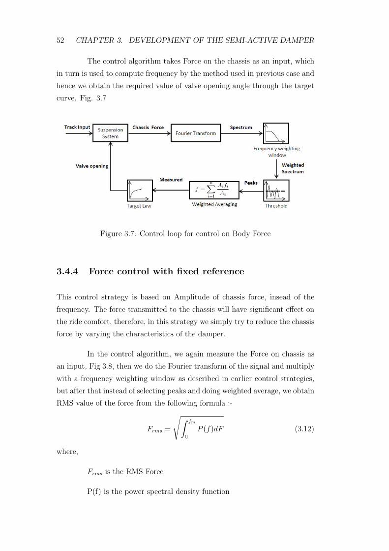
3.7 Control loop for control on Body Force . . . . . . . . . . . . . 52
3.8 Control loop for control on Body Force with a fixed reference . 53
LIST OF FIGURES vii
3.9 Stiffness and damping curves for hydraulic damper for sweep
input at 5mm amplitude and different valve opening angles . . 54
3.10 Selection of valve opening angles at different frequency based
on required stiffness and damping characteristics . . . . . . . . 55
3.11 Selection of valve opening angles at different frequency based
on required stiffness and damping characteristics . . . . . . . . 56
3.12 Track irregularity input . . . . . . . . . . . . . . . . . . . . . . 57
3.13 Track irregularity input with an added peak at 3hz . . . . . . 58
3.14 Track irregularity input with an added peak at 5hz . . . . . . 58
3.15 Comparative results for Track irregularity Input . . . . . . . . 60
3.16 Comparative results for Track irregularity input with an added
peak at 3hz . . . . . . . . . . . . . . . . . . . . . . . . . . . . 62
3.17 Comparative results for Track irregularity input with an added
peak at 5hz . . . . . . . . . . . . . . . . . . . . . . . . . . . . 64
4.1 Prototype of Semi-Active damper . . . . . . . . . . . . . . . . 66
4.2 Experimental setup of the semi-active damper . . . . . . . . . 67
4.3 Block diagram of the experimental setup . . . . . . . . . . . . 68
4.4 Valve operation for Track irregularity Input . . . . . . . . . . 70
4.5 Valve operation for Track irregularity with added peak at 3hz 70
4.6 Valve operation for Track irregularity with added peak at 5hz 71
4.7 Comparison of Numerical and Experimental results of valve
operation for Track irregularity Input . . . . . . . . . . . . . . 71
4.8 Comparison of Numerical and Experimental results of valve
operation for Track irregularity with added peak at 3hz . . . . 72
viii LIST OF FIGURES
4.9 Comparison of Numerical and Experimental results of valve
operation for Track irregularity with added peak at 5hz . . . . 72

List of Tables
2.1 Experimental setup for passive damper . . . . . . . . . . . . . 38
3.1 Selected valve opening angles for different frequencies . . . . . 56
3.2 RMS and Peak values for Track irregularity Input . . . . . . . 60
3.3 Normalized values for Track irregularity Input . . . . . . . . . 60
3.4 RMS and Peak values for Track irregularity input with an added
peak at 3hz . . . . . . . . . . . . . . . . . . . . . . . . . . . . 61
3.5 Normalized values for Track irregularity input with an added
peak at 3hz . . . . . . . . . . . . . . . . . . . . . . . . . . . . 62
3.6 RMS and Peak values for Track irregularity input with an added
peak at 5hz . . . . . . . . . . . . . . . . . . . . . . . . . . . . 63
3.7 Normalized values for Track irregularity input with an added
peak at 5hz . . . . . . . . . . . . . . . . . . . . . . . . . . . . 63
ix
Abstract
Hydraulic dampers are most widely used in the suspension system on trains
and heavy vehicles. However, they suffer from a major drawback resulting
from the change in characteristics of this device at high frequency, i.e. the
equivalent stiffness of the damper increases considerably at high frequency
along with a substantial decrease in the equivalent damping. This effect leads
to increase in the transmitted force at high frequency excitations, which has a
negative effect on the ride quality. To mitigate this effect, semi-active control
strategies for hydraulic dampers have been developed and tested.
This study evaluates the dynamic response of four semi-active con-
trol strategies as tested on a numerical model of a quarter-train system and
an experimental setup to test the performance of a single hydraulic damper.
Skyhook control strategy, which is most commonly used control strategy in
order to enhance comfort, is used as a reference for comparison. Each control
strategy is evaluated for its performance under different base excitations and
RMS acceleration on the chassis is used as a performance evaluation criterion
as it is the most commonly used parameter to evaluate comfort.
1
2 LIST OF TABLES
Acknowledgements
I would like to thank my supervisor, Professor Edoardo Sabbioni for his guid-
ance and kind support throughout the duration of the project. Special thanks
to Ing. Michele Vignati for working closely with me on this project, being
a helpful guide and providing all necessary information and help during the
project. I would also like to thank my parents, sister and my special person,
Alla, for being with me and for all the love and support. At last but not least,
my sincere gratitude to all other people who directly or indirectly helped me
to complete this project.
3

4 LIST OF TABLES
Introduction
Actively controlled suspensions have been widely studied theoretically and
experimentally for automobiles and rail vehicles. These studies have demon-
strated significant performance benefits. For railway vehicles, active suspen-
sions that deal primarily with improvement in ride quality are now starting
to be incorporated on a regular basis. Furthermore railway engineers are also
interested in using active control to achieve a functionality that is not possible
with a purely passive (mechanical) suspension. [1]
The present railway operators are facing intense pressure due to com-
petition from the air and road transport industries. In order for them to oper-
ate more efficiently and effectively, they are investigating ways to reduce the
traveling time, increase the number of passengers and reduce operating costs.
The trend of faster and lighter vehicles are ways in which these objectives can
be met. Therefore trains of the future will be designed with lighter bodies
and bogies to enable them to operate at a much higher speed. But as the
speed of the train is increased, it will lead to more high-frequency vibrations
which will certainly affect the ride quality and generate unacceptable levels of
internal noise.
The main objective of the project is to improve the high frequency
characteristics of a railway secondary suspension system, by incorporating an
electronic control system. By reducing the vibration at high frequencies, it
is possible to enhance the ride comfort for the passengers. There are conven-
tional control strategies, already available in literature to attain this objective,
for example, a Skyhook control loop. In this project, other possible control
strategies are studied and compared with a conventional skyhook strategy on
the basis of the most relevant performance criterion to determine the best
5
6 LIST OF TABLES
solution for achieving our objective.
In the first chapter, ”State of the art”, we discuss about the design
of a suspension system, the various constraints and limitations. Then we talk
about how to manage these constraints using an actively controlled suspen-
sion, conventional control strategies i.e. skyhook, different types of active sus-
pensions, their relative advantages and disadvantages, the latest technological
advancements and research in the field of active suspensions and also about
the most commonly used parameter to judge the performance of a suspension
system.
Then in the second chapter, ”Model of the passive damper”, we de-
scribe the numerical model of the passive damper using various mathematical
equations and formulas. This model is used for numerical simulation using
Matlab and Simulink. Then we describe the Experimental setup used for
characterization of the passive damper and also for validation of the numeri-
cal model.
In the third chapter, ”Development of the semi-active damper”, we
discuss the numerical model for the semi-active damper and the Quarter-
Train model used for analysis purpose. Then we introduce 4 different control
strategies which we designed, as explained with the help of block diagrams
and schematics showing how they can be implemented actually in a physical
model. Then we discuss the Input excitation methods used and the results
from the Quarter - Train model with semi-active damper. We also describe the
method adopted for determination of the correlation curve between frequency
and required valve opening.
In the fourth chapter, ”Prototype of the semi-active damper”, we
describe the physical prototype of the semi-active damper which we created
for physical testing of the proposed solution. We talk about the experimental
setup created for testing and evaluation of the physical prototype and the
results from the testing compared with numerical model.
Then in the last chapter, we summarize all our observations and find-
ings from various numerical and physical tests conducted, comparison between
different control strategies and try to find the best possible solution.

Chapter 1
State of the Art
The automotive suspension is a compromise between the conflicting demand
of ride handling and vehicle stability [2]. The primary function of a suspension
is to isolate the occupants of the vehicle from the accelerations generated in
the vehicle by track irregularities. These irregularities arise as a result of
construction tolerances, and the degradation which occurs in the track due to
use and exposure to the elements. While the original need to isolate the vehicle
from track irregularities is to enhance the ride comfort of the passengers, there
is an equal need to protect the track from the impact of the vehicles using it
as this can lead to rapid deterioration and high maintenance costs.
When a suspension is isolating a vehicle from track irregularities, it
must also allow the vehicle to follow intentional long wavelength features in
the track, where it is following contours in the landscape. Thus a suspension is
a low pass filter which enables a vehicle to follow the long wavelength features
that are designed into the track, while isolating it from the short wavelength
features which arise as a result of construction tolerances and wear and tear.
In order to provide maximum isolation in a vehicle it is necessary
to allow the wheels to follow the vertical profile of the road while the vehicle
body remains at a fixed height in space. In practice the body cannot remain at
a fixed height in space as this produces a requirement for infinite suspension
travel. Consequently the degree of isolation produced by a suspension is a
function of the amount of suspension travel available.
7
8 CHAPTER 1. STATE OF THE ART
1.1 Design Constraints
When designing a suspension the two major variables available to the suspen-
sion designer are damping rate and spring rate. For estimation of comfort level
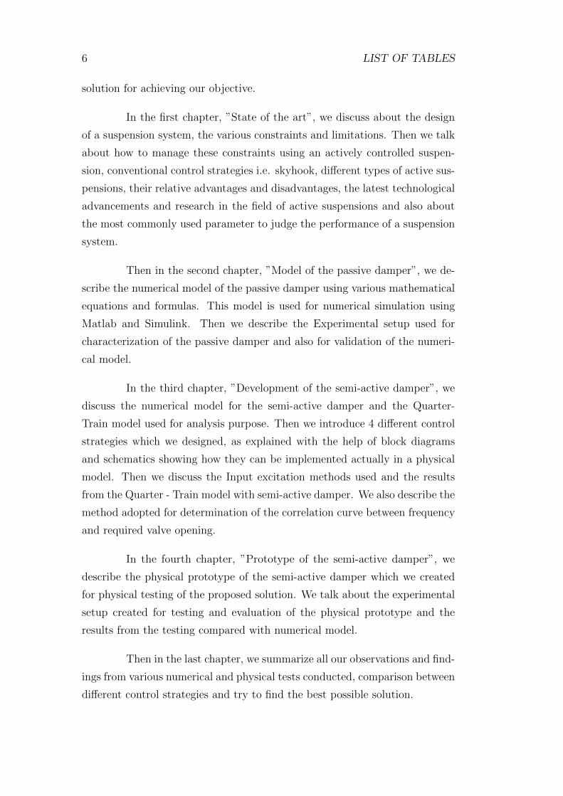
of the passengers, body acceleration is considered the best indicator [3] [4] .
Fig.1.1 shows the effect of varying the damping rate from the nominal val-
ues appropriate to a train, when it is driven over a track with a profile given
in [2] [5]. At low damping rates there is a large peak in the body acceleration
at the frequency of chassis mode (1 Hz), and a smaller one at the frequency
of bogie mode (8 Hz). Increasing the damping rate, reduces the acceleration
at frequencies of chassis mode while increasing it at high frequencies, creating
an optimum damping rate for minimum acceleration. If the damping rate be-
comes very high, the acceleration at chassis mode reduces and at bogie mode
becomes high. Consequently, in order to ensure a good ride, the damping rate
has to be a compromise.
Figure 1.1: Effect of damper rate on body acceleration
Also, for a fixed damper with chosen optimized parameters, the stiff-
ness and damping changes with the frequency of the vibration input. While
stiffness increases with increase in frequency, damping rate reduces as shown
in Fig 1.2 , therefore the energy transmitted to the chassis increases at higher
frequencies, so at higher train speeds. This can be quantified in form of a

1.1. DESIGN CONSTRAINTS 9
parameter called Transmissibility, defined by eq.1.1
τ =√k2 + ω2r2 (1.1)
where,
k = Stiffness of the damper
ω = Frequency of vibration
r = Damping
Transmissibility increases with increase in frequency as shown in
Fig.1.3 The main aim of the project is to reduce the energy tansmitted to
the chassis at high frequencies, therefore to reduce the transmissibility.
Figure 1.2: Effect of frequency on stiffness and damping rate
Figure 1.3: Variation of transmissibility with frequency in a passive damper
10 CHAPTER 1. STATE OF THE ART
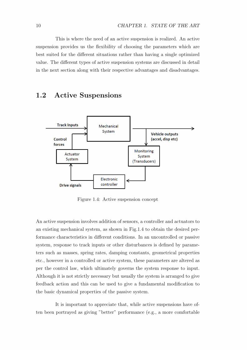
This is where the need of an active suspension is realized. An active
suspension provides us the flexibility of choosing the parameters which are
best suited for the different situations rather than having a single optimized
value. The different types of active suspension systems are discussed in detail
in the next section along with their respective advantages and disadvantages.
1.2 Active Suspensions
Figure 1.4: Active suspension concept
An active suspension involves addition of sensors, a controller and actuators to
an existing mechanical system, as shown in Fig.1.4 to obtain the desired per-
formance characteristics in different conditions. In an uncontrolled or passive
system, response to track inputs or other disturbances is defined by parame-
ters such as masses, spring rates, damping constants, geometrical properties
etc., however in a controlled or active system, these parameters are altered as
per the control law, which ultimately governs the system response to input.
Although it is not strictly necessary but usually the system is arranged to give
feedback action and this can be used to give a fundamental modification to
the basic dynamical properties of the passive system.
It is important to appreciate that, while active suspensions have of-
ten been portrayed as giving ”better” performance (e.g., a more comfortable

1.3. CLASSIFICATION 11
ride quality when applied to a vehicle’s secondary suspension; enhanced bogie
stability and/or more effective curving when applied to the primary suspen-
sion), what they really offer is a better trade-off in the design process, for
example between ride quality and suspension deflection, or between stability
and curving. How the suspension engineer chooses to use the increased de-
sign freedom which this provides, depends upon the application. The concept
enables a number of approaches to be used which are either impossible or
impracticable with passive suspensions.
1.3 Classification
Active Suspensions have a very vast field and there is a great variety of oppor-
tunities and possibilities, therefore it is useful to provide some sort of classifi-
cation to identify the distinctness of some of the issues and also to emphasize
the control options which are available. Three broad classification categories
are introduced - the scope, the degree, and the technology of control. [1]
Scope of control identifies the modes of the suspension which are being
controlled by the active suspension. Note that, due to the interactive
dynamic nature of a railway vehicle, a number of modes may be in-
fluenced by a particular design, but this refers to those modes whose
response is deliberately being addressed by the control action.
Degree of control defines the type and dynamic range of the control action.
Two broad categories in this respect are Semi-Active and Full-Active
control as shown in Fig. 1.5.

12 CHAPTER 1. STATE OF THE ART
Figure 1.5: Semi Active and Fully Active suspension
In semi-active control the characteristics of an otherwise passive element
(mostly a damper, but not inevitably so) are varied rapidly on the basis
of measurements of variables within the dynamic system and the control
strategy employed. Closely related is an option known variously as semi-
passive, adjustable passive and adaptive, in which the characteristics are
varied on the basis of a variable which is not influenced by the dynamic
system being controlled - a good example is varying the rate of the
damper as a function of vehicle speed.
In full-active control, actuators are used which are either to completely
replace or augment passive elements, and the force they produce is var-
ied according to measurements from the system and control law. A
full-active system must have an external source of power to supply the
actuators (in addition to low level power supplies associated with the
control electronics which are inevitable with any form of active suspen-
sion). There is another aspect to the degree of control, primarily appli-
cable to full-active suspensions, which can broadly be subdivided into
low bandwidth or high bandwidth. In low bandwidth systems there will
be passive elements which dictate the fundamental dynamic response,
and the function of the active element is associated with some low fre-
quency activity such as leveling or centering. This restriction enables

1.3. CLASSIFICATION 13
some reduction in force and/or velocity requirement for the actuators.
By contrast, high bandwidth active systems have a much enhanced ca-
pability, and the overall dynamic response will primarily be determined
by the active control strategy, which will probably act throughout the
frequency range which is relevant to the particular suspension function
being controlled.
A semi active suspension is a valid engineering solution when it can
reasonably approximate the performance of the active control because it
requires a low power controller that can be easily realized at a lower cost
than that of a fully active one. Note, however, that a semi active system
clearly lacks other important secondary advantages of the fully active
one, namely the ability to resist downward static forces due to passenger
and baggage loads and to control the altitude of the vehicle. [6]
Technology of Control concerns the practicalities of implementation, and
strictly covers the controller, the sensors and the actuators. The avail-
ability of remarkable quantities of computing power means that the
controller is unlikely to be a limiting factor in the implementation, al-
though issues such as reliability, ruggedness etc. cannot be ignored. The
sensors are probably a significantly more important issue, but a large
variety of suitable types is available, and the key aspects here relate
to reliability and cost. The provision of high reliability actuation of
sufficient performance is one of the main challenges in active suspen-
sions. Cost of the total system (i.e., including power sources, etc.) is
certainly important but ease of installation (compactness, etc.), main-
tainability and maintenance cost, reliability and failure modes must all
have essential inputs into the process of choosing and procuring the ac-
tuator system. Actuator technologies which are possible for active sus-
pensions are servo-hydraulic, servo-pneumatic, electro-mechanical and
electro-magnetic. Servo-hydraulic actuators themselves are compact and
easy to fit, but the whole system tends to be bulky and inefficient, and
there are important questions relating to maintainability. Pneumatic ac-
tuators are a possibility, particularly since the airsprings fitted to many
railway vehicles can form the basic actuator, but inefficiency and limited
controllability are important restrictions. Electro-mechanical actuators
offer a technology with which the railway is generally familiar, and the

14 CHAPTER 1. STATE OF THE ART
availability of high performance servo-motors and high efficiency power
electronics are favorable indicators. However they tend to be less com-
pact and the reliability and life of the mechanical components needs
careful consideration. Electro-magnetic actuators potentially offer an
extremely high reliability and high performance solution, but they tend
to be quite bulky and have a somewhat limited travel.
1.4 Types of Active/Semi-Active Dampers
1.4.1 Active Dampers
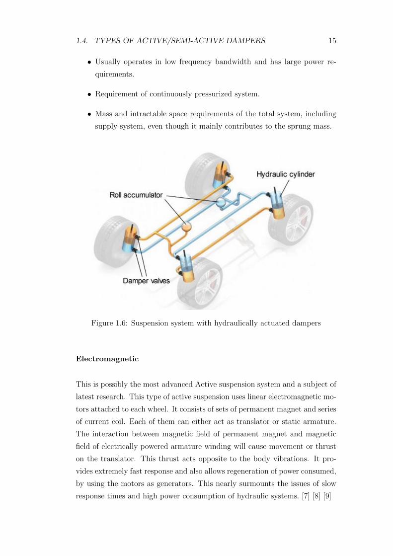
Hydraulic Actuated
Hydraulically actuated suspensions are controlled with the use of hydraulic
servomechanisms. The hydraulic pressure to the servos is supplied by a high
pressure radial piston hydraulic pump. Sensors continually monitor body
movement and vehicle ride level, constantly supplying the computer with new
data. As the computer receives and processes data, it operates the hydraulic
servos, mounted beside each wheel. Almost instantly, the servo-regulated
suspension generates counter forces to body vibrations. In practice, the system
always have the desirable self-leveling and height adjusting features, with the
latter now tied to vehicle speed for improved aerodynamic performance, as
the vehicle lowers itself at high speed.
Benefits:
• Better ride quality specially on highly undulated surface as it is very
effective in controlling Roll motion.
• High damping forces can be obtained.
• Ease of design and control.
Drawbacks
1.4. TYPES OF ACTIVE/SEMI-ACTIVE DAMPERS 15
• Usually operates in low frequency bandwidth and has large power re-
quirements.
• Requirement of continuously pressurized system.
• Mass and intractable space requirements of the total system, including
supply system, even though it mainly contributes to the sprung mass.
Figure 1.6: Suspension system with hydraulically actuated dampers
Electromagnetic
This is possibly the most advanced Active suspension system and a subject of
latest research. This type of active suspension uses linear electromagnetic mo-
tors attached to each wheel. It consists of sets of permanent magnet and series
of current coil. Each of them can either act as translator or static armature.
The interaction between magnetic field of permanent magnet and magnetic
field of electrically powered armature winding will cause movement or thrust
on the translator. This thrust acts opposite to the body vibrations. It pro-
vides extremely fast response and also allows regeneration of power consumed,
by using the motors as generators. This nearly surmounts the issues of slow
response times and high power consumption of hydraulic systems. [7] [8] [9]

16 CHAPTER 1. STATE OF THE ART
Benefits:
• Extremely fast response.
• Low power consumption due to regeneration and large frequency band-
width.
• Higher efficiency
• Improved stability and dynamic behavior
• Accurate force control;
Drawbacks
• Relatively complex and expensive system.
Figure 1.7: Electro-mechanical Active damper
1.4.2 Semi-Active Dampers
Continuously Controlled Damping (CCD)
CDC is an electronic damping system, where a control unit takes the input
from various sensors measuring body, wheel and lateral acceleration and use
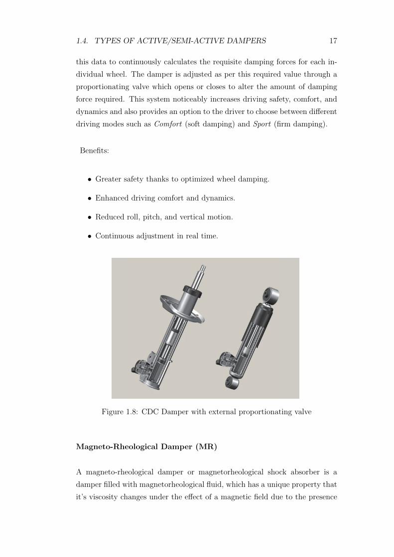
1.4. TYPES OF ACTIVE/SEMI-ACTIVE DAMPERS 17
this data to continuously calculates the requisite damping forces for each in-
dividual wheel. The damper is adjusted as per this required value through a
proportionating valve which opens or closes to alter the amount of damping
force required. This system noticeably increases driving safety, comfort, and
dynamics and also provides an option to the driver to choose between different
driving modes such as Comfort (soft damping) and Sport (firm damping).
Benefits:
• Greater safety thanks to optimized wheel damping.
• Enhanced driving comfort and dynamics.
• Reduced roll, pitch, and vertical motion.
• Continuous adjustment in real time.
Figure 1.8: CDC Damper with external proportionating valve
Magneto-Rheological Damper (MR)
A magneto-rheological damper or magnetorheological shock absorber is a
damper filled with magnetorheological fluid, which has a unique property that
it’s viscosity changes under the effect of a magnetic field due to the presence
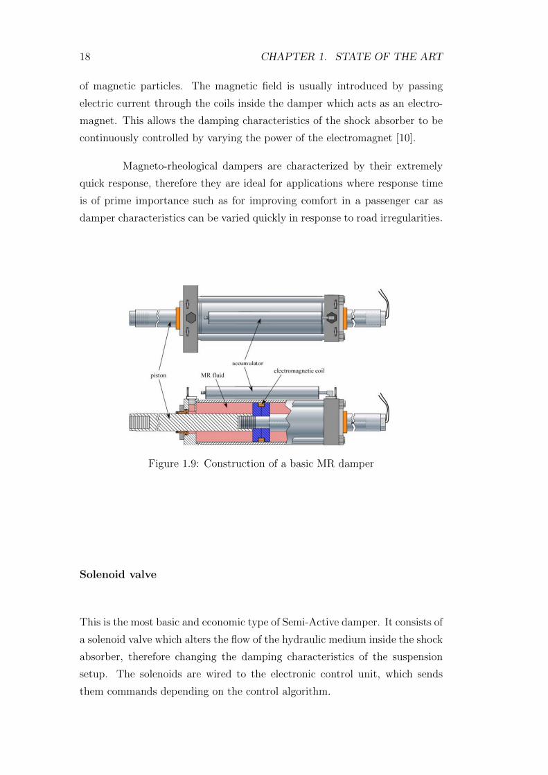
18 CHAPTER 1. STATE OF THE ART
of magnetic particles. The magnetic field is usually introduced by passing
electric current through the coils inside the damper which acts as an electro-
magnet. This allows the damping characteristics of the shock absorber to be
continuously controlled by varying the power of the electromagnet [10].
Magneto-rheological dampers are characterized by their extremely
quick response, therefore they are ideal for applications where response time
is of prime importance such as for improving comfort in a passenger car as
damper characteristics can be varied quickly in response to road irregularities.
Figure 1.9: Construction of a basic MR damper
Solenoid valve
This is the most basic and economic type of Semi-Active damper. It consists of
a solenoid valve which alters the flow of the hydraulic medium inside the shock
absorber, therefore changing the damping characteristics of the suspension
setup. The solenoids are wired to the electronic control unit, which sends
them commands depending on the control algorithm.
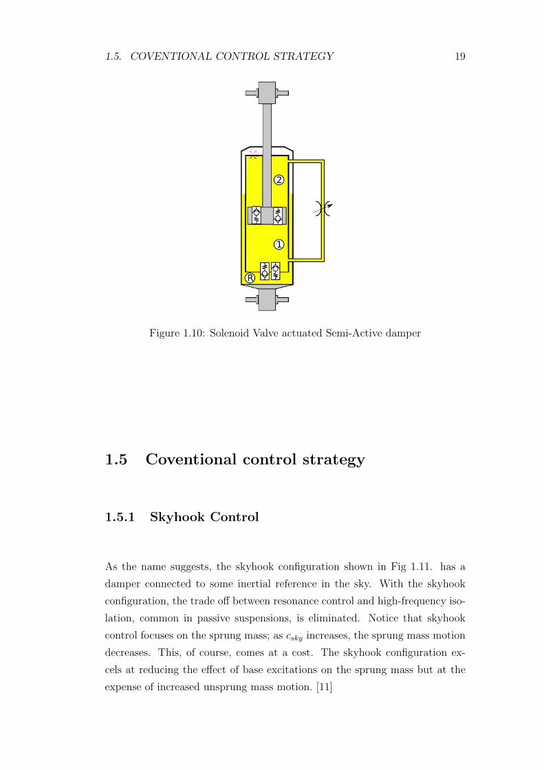
1.5. COVENTIONAL CONTROL STRATEGY 19
Figure 1.10: Solenoid Valve actuated Semi-Active damper
1.5 Coventional control strategy
1.5.1 Skyhook Control
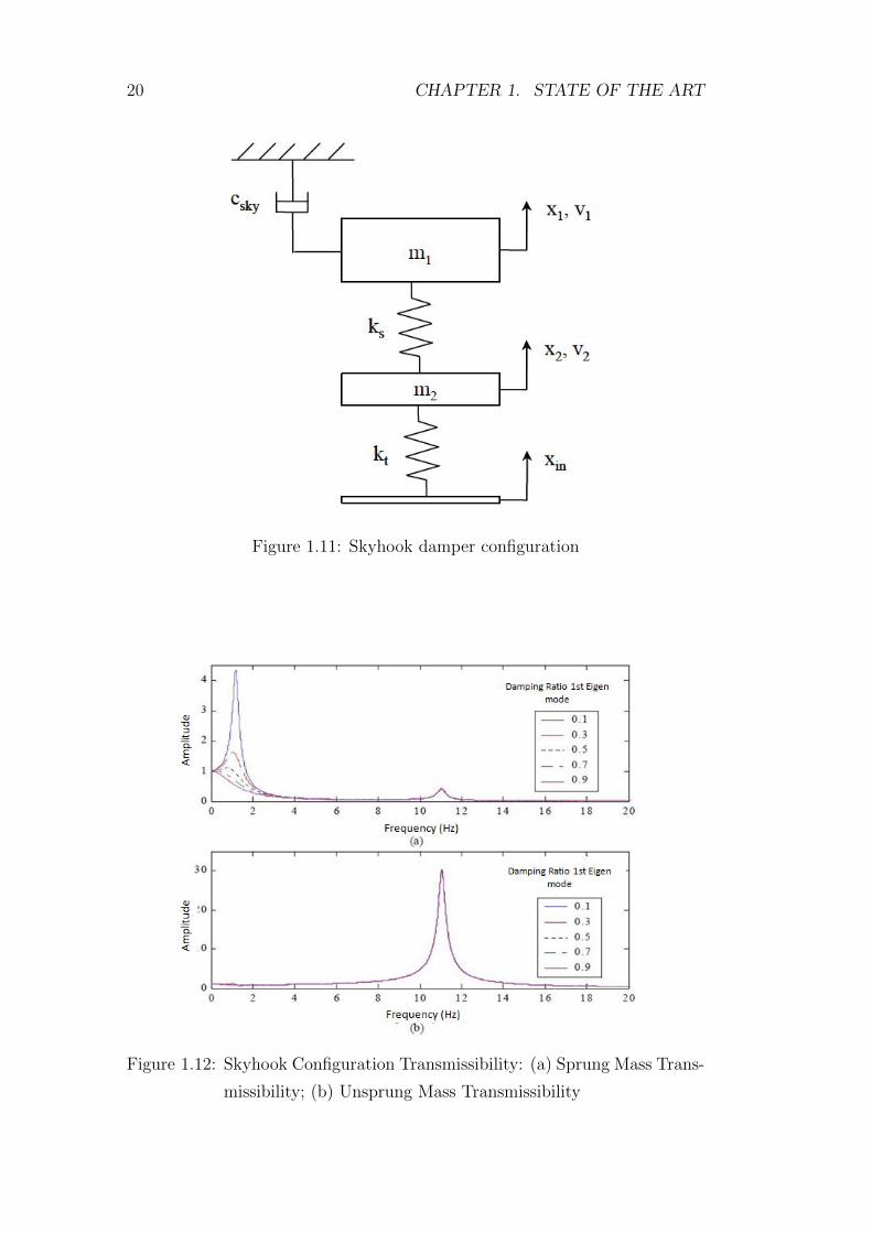
As the name suggests, the skyhook configuration shown in Fig 1.11. has a
damper connected to some inertial reference in the sky. With the skyhook
configuration, the trade off between resonance control and high-frequency iso-
lation, common in passive suspensions, is eliminated. Notice that skyhook
control focuses on the sprung mass; as csky increases, the sprung mass motion
decreases. This, of course, comes at a cost. The skyhook configuration ex-
cels at reducing the effect of base excitations on the sprung mass but at the
expense of increased unsprung mass motion. [11]
20 CHAPTER 1. STATE OF THE ART
Figure 1.11: Skyhook damper configuration
Figure 1.12: Skyhook Configuration Transmissibility: (a) Sprung Mass Trans-
missibility; (b) Unsprung Mass Transmissibility
1.5. COVENTIONAL CONTROL STRATEGY 21
The transmissibility for this system is shown in Fig 1.12. for differ-
ent values of the skyhook-damping coefficient,csky. Notice that as the skyhook
damping ratio increases, the resonant transmissibility near ωn1 decreases, even
to the point of isolation, but the transmissibility near ωn2 increases. In essence,
this skyhook configuration is adding more damping to the sprung mass and
taking away damping from the unsprung mass. The skyhook configuration is
ideal if the primary goal is isolating the sprung mass from base excitations,
even at the expense of excessive unsprung mass motion. An additional ben-
efit is apparent in the frequency range between the two natural frequencies.
With the skyhook configuration, isolation in this region actually increases with
increasing csky.
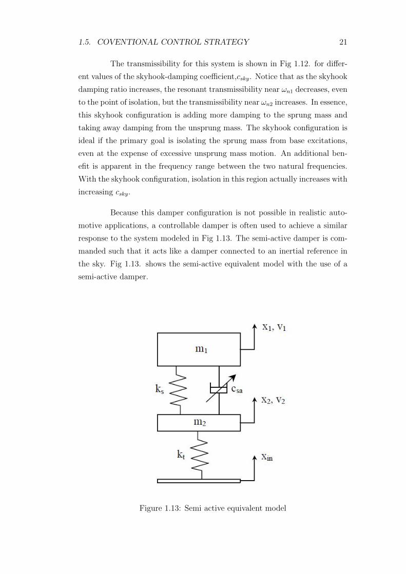
Because this damper configuration is not possible in realistic auto-
motive applications, a controllable damper is often used to achieve a similar
response to the system modeled in Fig 1.13. The semi-active damper is com-
manded such that it acts like a damper connected to an inertial reference in
the sky. Fig 1.13. shows the semi-active equivalent model with the use of a
semi-active damper.
Figure 1.13: Semi active equivalent model

22 CHAPTER 1. STATE OF THE ART
Several methods exist for representing the equivalent skyhook damp-
ing force with the configuration shown in Fig 1.13. Perhaps the most compre-
hensive way to arrive at the equivalent skyhook damping force is to examine
the forces on the sprung mass under several conditions. First, let us define
certain parameters and conventions that will be used throughout controller
development. Referring to Fig 1.13., the relative velocity, v12 = (v1 − v2), is
defined as the velocity of the sprung mass(m1) relative to the unsprung mass
(m2). When the two masses are separating,v12 is positive. For all other cases,
up is positive and down is negative.
Now, with these definitions, let us consider the case when the sprung
mass is moving upwards and the two masses are separating. Under the ideal
skyhook configuration we find that the force due to the skyhook damper is
Fsky = −cskyv1 (1.2)
where Fsky is the skyhook damping force. Next we examine the semi-active
equivalent model and find that the damper is in tension and the damping force
due to the semi-active damper is
Fsa = −csav12 (1.3)
where Fsa is the semi-active damping force. Now, in order for the semi-active
equivalent model to perform like the skyhook model, the damping forces must
be equal, or
Fsky = −cskyv1 = −csav12 = Fsa (1.4)
We can solve for the semi-active damping in terms of the skyhook damping (
eq 1.5.) and use this to find the semi-active damping force needed to represent
skyhook damping when both v1 and v12 are positive (eq 1.6.)
csa =cskyv1
v12
(1.5)
Fsa = cskyv1 (1.6)
Next, let us consider the case when both v1 and v12 are negative. Now the
sprung mass is moving down and the two masses are coming together. In this
scenario, the skyhook damping force would be in the positive direction, or
Fsky = cskyv1 (1.7)

1.5. COVENTIONAL CONTROL STRATEGY 23
Likewise, because the semi-active damper is in compression, the force due to
the semi-active damper is also positive, or
Fsa = csav12 (1.8)
Following the same procedure as the first case, equating the damping forces
reveals the same semi-active damping force as the first case. Thus, we can
conclude that when the product of the two velocities is positive, the semi-
active force is defined by eq 1.6.
Now consider the case when the sprung mass is moving upwards
and the two masses are coming together. The skyhook damper would again
apply a force on the sprung mass in the negative direction. In this case, the
semi-active damper is in compression and cannot apply a force in the same
direction as the skyhook damper. For this reason, we would want to minimize
the damping, thus minimizing the force on the sprung mass.
The final case to consider is the case when the sprung mass is moving
downwards and the two masses are separating. Again, under this condition the
skyhook damping force and the semi-active damping force are not in the same
direction. The skyhook damping force would be in the positive direction, while
the semi-active damping force would be in the negative direction. The best
that can be achieved is to minimize the damping in the semi-active damper.
Summarizing these four conditions, we arrive at the well-known semi-
active skyhook control policy:v1v12 ≥ 0, Fsa = cskyv1
v1v12 < 0, Fsa = 0(1.9)
It is worth emphasizing that when the product of the two velocities is positive
that the semi-active damping force is proportional to the velocity of the sprung
mass. Otherwise, the semi-active damping force is at a minimum.
It is preferable to add another component to the damping force pro-
vided by the actuator that is related to the passive behavior of the damper
and is proportional to the relative speed of the chassis with respect to the
chassis, described in eq 1.10. This component is added as a precautionary
measure to provide damping force in case of a breakdown and to also damp
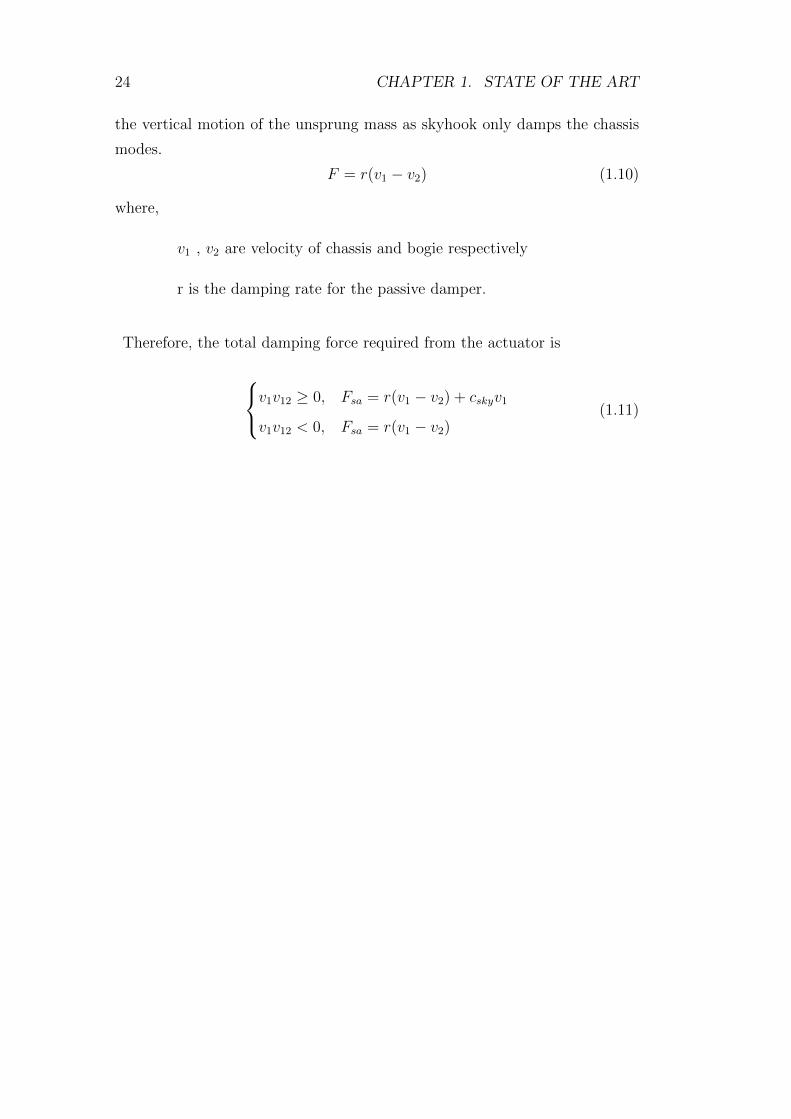
24 CHAPTER 1. STATE OF THE ART
the vertical motion of the unsprung mass as skyhook only damps the chassis
modes.
F = r(v1 − v2) (1.10)
where,
v1 , v2 are velocity of chassis and bogie respectively
r is the damping rate for the passive damper.
Therefore, the total damping force required from the actuator is
v1v12 ≥ 0, Fsa = r(v1 − v2) + cskyv1
v1v12 < 0, Fsa = r(v1 − v2)(1.11)

Chapter 2
Model of Passive Damper
2.1 Numerical Model
A numerical model of the damper is required as it enables us to do our pre-
liminary study about the damper characteristics, its behavior under different
parameters such as displacement amplitude and frequency of input excitation.
It also provides a feasible and more efficient way of testing and analyzing our
control strategies through numerical simulation rather than depending upon
experimental setup always. In this manner, we can predict errors at earlier
stages and we can also perform more advanced analysis on a Quarter-train
model which is complex to replicate experimentally.
The Hydralic damper can have different configurations as described
below [12] :-
1. Single Acting piston:
Figure 2.1: Single-Acting piston type hydraulic damper
25
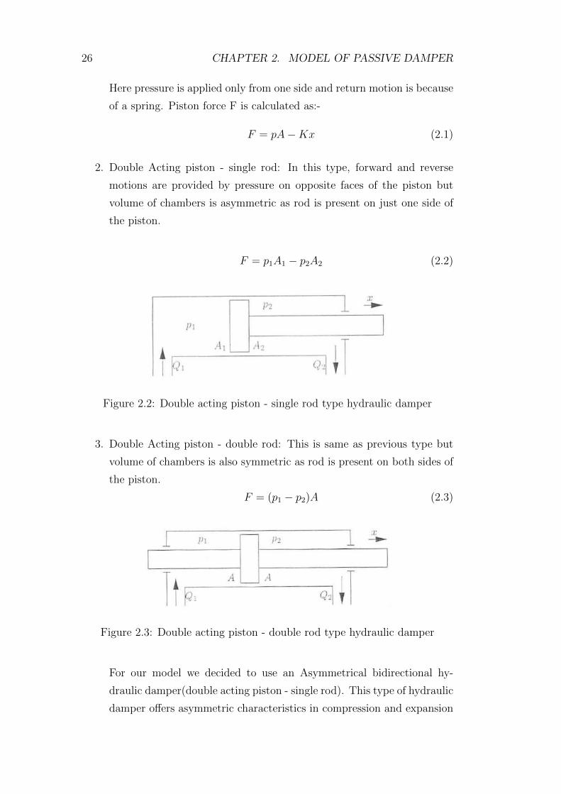
26 CHAPTER 2. MODEL OF PASSIVE DAMPER
Here pressure is applied only from one side and return motion is because
of a spring. Piston force F is calculated as:-
F = pA−Kx (2.1)
2. Double Acting piston - single rod: In this type, forward and reverse
motions are provided by pressure on opposite faces of the piston but
volume of chambers is asymmetric as rod is present on just one side of
the piston.
F = p1A1 − p2A2 (2.2)
Figure 2.2: Double acting piston - single rod type hydraulic damper
3. Double Acting piston - double rod: This is same as previous type but
volume of chambers is also symmetric as rod is present on both sides of
the piston.
F = (p1 − p2)A (2.3)
Figure 2.3: Double acting piston - double rod type hydraulic damper
For our model we decided to use an Asymmetrical bidirectional hy-
draulic damper(double acting piston - single rod). This type of hydraulic
damper offers asymmetric characteristics in compression and expansion

2.1. NUMERICAL MODEL 27
due to difference in the volume of the two main chambers, but is lighter
in construction and more compact. Therefore, considering the need of a
physical prototype at later stage, this is an effective solution.
A hydraulic damper can be broadly described as a cylindrical part as
shown in figure 2.4, with two main chambers (chamber 1 and chamber 2) filled
with a viscous fluid and separated by a piston with an internal valve (Valve A)
to regulate the passage of fluid from one chamber to other. The flow of fluid
through a valve is regulated as per the valve characteristics in compression
and expansion and on the pressure difference between the 2 chambers.
Other than two main chambers, there is another chamber connected
to main chamber by valve B which accounts for flow of fluid around the rod
due to leakage and there is also a reserve chamber connected by valve C which
holds extra reserve of fluid. All these valves have different characteristics
depending upon their design. In this section we describe the numerical model
of the hydraulic damper through mathematical equations and formula.
Figure 2.4: Model of a hydraulic damper

28 CHAPTER 2. MODEL OF PASSIVE DAMPER
V1 , V2 are the volumes of chamber 1 and 2
p1 , p2 are the fluid pressures inside chamber 1 and 2
V01 and V02 are the initial volumes of the 2 chambers
mp is the mass of the piston
mr is the mass of the piston rod
Ap is the area of piston
Ar is the area of the piston rod
zG , zE and zF are position of points G, E and F from reference
hp is the thickness of the piston
QA , QB and QC are fluid flow rates through valve A,B and C.
Pressure dynamics in compression chamber (chamber 1) and rebound
chamber (chamber 2) can be explained by the equations below [13] [12]:
V1
β1
p1 = −V1 −QA +QC (2.4)
V2
β2
p2 = −V2 +QA +QB (2.5)
where,
β1 , β2 = β is isothermal bulk modulus of the fluid, this parameter
defines compressibility of the fluid, higher the value of β , lower is the
compressibility.
volumes of chambers are:
V1 = V01 + Ap(zG − zF −hP2
) (2.6)
V2 = V02 + (Ap − Ar)(zE − zG +hP2
) (2.7)
2.1. NUMERICAL MODEL 29
volumes time derivatives:
V1 = Ap( ˙zG − zF ) (2.8)
V2 = (Ap − Ar)( ˙zE − ˙zG) (2.9)
piston force
Famm = −(p1Ap − p2(Ap − Ar))− (mp +mr)zG (2.10)
The flow through the valves is expected to be turbulent due to high
viscosity of fluid and fast excitation due to road irregularities which
increases flow speed. Turbulent flow A and C are evaluated as:
Q = cqAv
√2|∆p|ρ
.sign(∆p) (2.11)
where
cq = cq,max. tanh(2λ
λcric) (2.12)
λ =hdν
√2∆p
ρ, hd =
√4Avπ
(2.13)
λcrit is the critical flow number at which transfer from laminar to tur-
bulent characteristic occurs.
cq is the discharge coefficient
Av is the minimum area of the orifice cross section
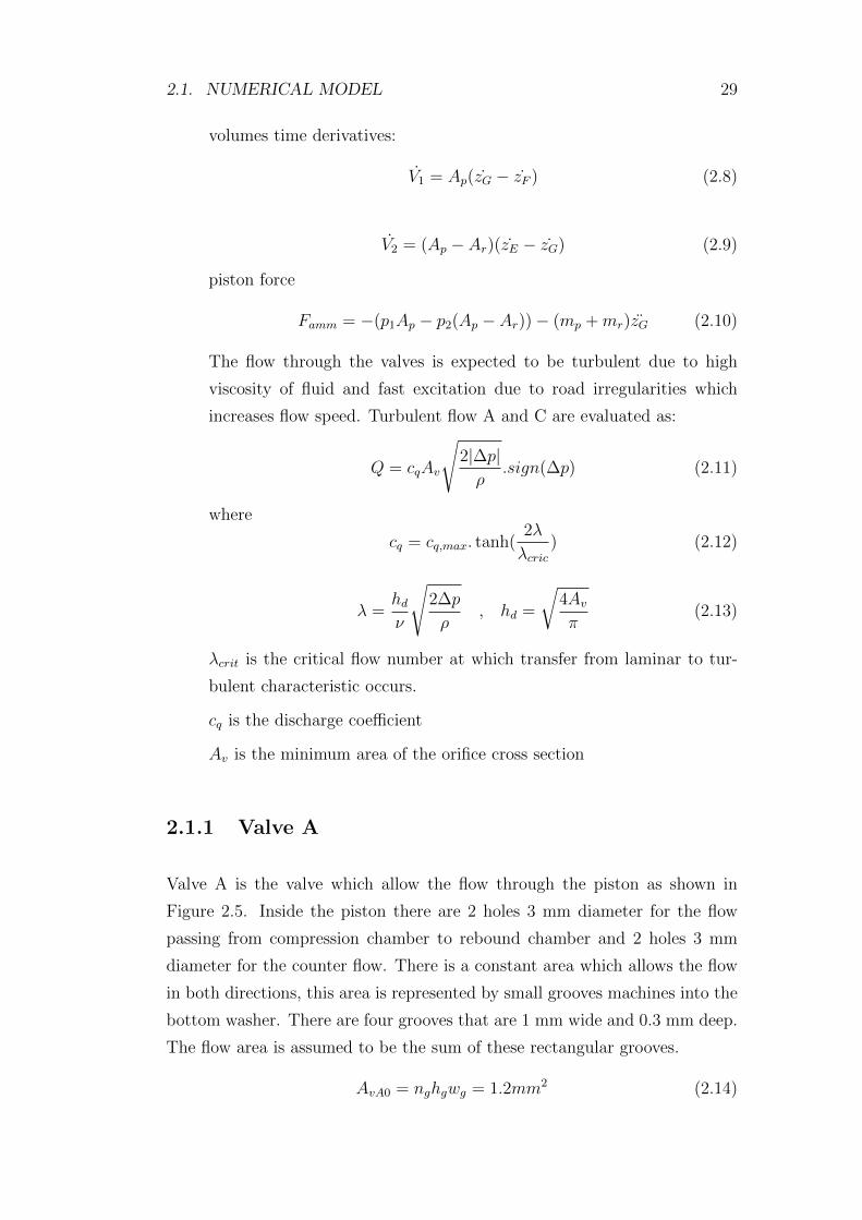
2.1.1 Valve A
Valve A is the valve which allow the flow through the piston as shown in
Figure 2.5. Inside the piston there are 2 holes 3 mm diameter for the flow
passing from compression chamber to rebound chamber and 2 holes 3 mm
diameter for the counter flow. There is a constant area which allows the flow
in both directions, this area is represented by small grooves machines into the
bottom washer. There are four grooves that are 1 mm wide and 0.3 mm deep.
The flow area is assumed to be the sum of these rectangular grooves.
AvA0 = nghgwg = 1.2mm2 (2.14)

30 CHAPTER 2. MODEL OF PASSIVE DAMPER
where,
ng is the number of grooves.
hg is the depth of the grooves.
wg is the width of the grooves.
When the damper is in compression stroke, the difference of pressure
between compression chamber (chamber 1) and rebound chamber (chamber
2) makes the top washer move upward compressing the spring. In this case
the flow area is a circular surface whose perimeter is the product of the cir-
cumference of flow diameter (dflow = 25 mm) times the lift of the valve which
depends on pressure gap.
AvAl = πdflowl (2.15)
where,
l is the lift of the valve.
The maximum lift is equal to spring height which is 2 mm thus the
maximum area is
AvAlmax = πdflowmaxlmax = 157mm2 (2.16)
The lift of the valve depends on spring compression. The force on the spring
is
F = (p1 − p2)π(d2
flow − d2i )
4(2.17)
where, F0 = kl0, which is the initial compression load of the spring di =
14.5mm is the inner diameter of washer; while the lift is
l =F − F0
k=
(p1 − p2)π(d2flow − d2
i )
4k− F0
k(2.18)
where k = 35 kN/m is the spring stiffness. Obviously the lift of the valve
cannot be lower than zero, this mean that the valve start opening only when
pressure force is higher than the static load.
l = 0 ⇒(p1 − p2)π(d2
flow − d2i )
4= kl0 = 140N (2.19)
The free length of the spring is 19 mm while the working length is 13 mm,
the initial compression is thus l0 = 4 mm; the minimum pressure difference

2.1. NUMERICAL MODEL 31
to lift the valve is
(p1 − p2)min =4kl0
π(d2flow − d2
i )= 0.64MPa (2.20)
The pressure difference to which corresponds the maximum displacement of
the spring is
(p1 − p2)max =klmax
π(d2flow−d2i )
4
(2.21)
Figure 2.5: Valve A: Piston mechanism
32 CHAPTER 2. MODEL OF PASSIVE DAMPER
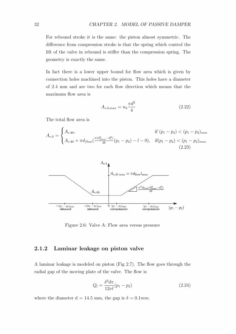
For rebound stroke it is the same: the piston almost symmetric. The
difference from compression stroke is that the spring which control the
lift of the valve in rebound is stiffer than the compression spring. The
geometry is exactly the same.
In fact there is a lower upper bound for flow area which is given by
connection holes machined into the piston. This holes have a diameter
of 2.4 mm and are two for each flow direction which means that the
maximum flow area is
AvA,max = nhπd2
4(2.22)
The total flow area is
AvA =
AvA0, if (p1 − p2) < (p1 − p2)min
AvA0 + πdflow(π(d2flow−d
2i )
4k(p1 − p2)− l − 0), if(p1 − p2) < (p1 − p2)max
(2.23)
Figure 2.6: Valve A: Flow area versus pressure
2.1.2 Laminar leakage on piston valve
A laminar leakage is modeled on piston (Fig 2.7). The flow goes through the
radial gap of the moving plate of the valve. The flow is
Ql =δ3dπ
12νl(p1 − p2) (2.24)
where the diameter d = 14.5 mm, the gap is δ = 0.1mm.
2.1. NUMERICAL MODEL 33
Figure 2.7: Piston laminar leakage
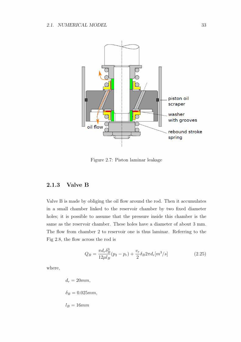
2.1.3 Valve B
Valve B is made by obliging the oil flow around the rod. Then it accumulates
in a small chamber linked to the reservoir chamber by two fixed diameter
holes; it is possible to assume that the pressure inside this chamber is the
same as the reservoir chamber. These holes have a diameter of about 3 mm.
The flow from chamber 2 to reservoir one is thus laminar. Referring to the
Fig 2.8, the flow across the rod is
QB =πdrδ
3B
12µlB(p2 − pr) +
vr2δB2πdr[m
3/s] (2.25)
where,
dr = 20mm,
δB = 0.025mm,
lB = 16mm
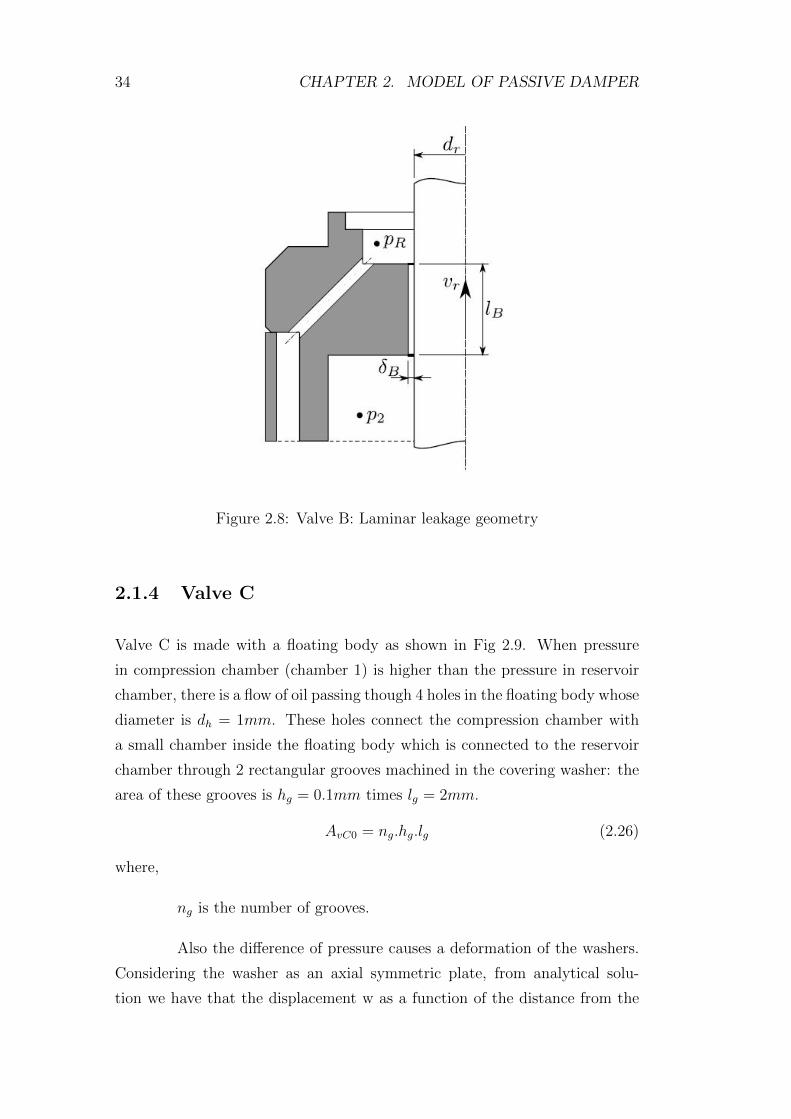
34 CHAPTER 2. MODEL OF PASSIVE DAMPER
Figure 2.8: Valve B: Laminar leakage geometry
2.1.4 Valve C
Valve C is made with a floating body as shown in Fig 2.9. When pressure
in compression chamber (chamber 1) is higher than the pressure in reservoir
chamber, there is a flow of oil passing though 4 holes in the floating body whose
diameter is dh = 1mm. These holes connect the compression chamber with
a small chamber inside the floating body which is connected to the reservoir
chamber through 2 rectangular grooves machined in the covering washer: the
area of these grooves is hg = 0.1mm times lg = 2mm.
AvC0 = ng.hg.lg (2.26)
where,
ng is the number of grooves.
Also the difference of pressure causes a deformation of the washers.
Considering the washer as an axial symmetric plate, from analytical solu-
tion we have that the displacement w as a function of the distance from the
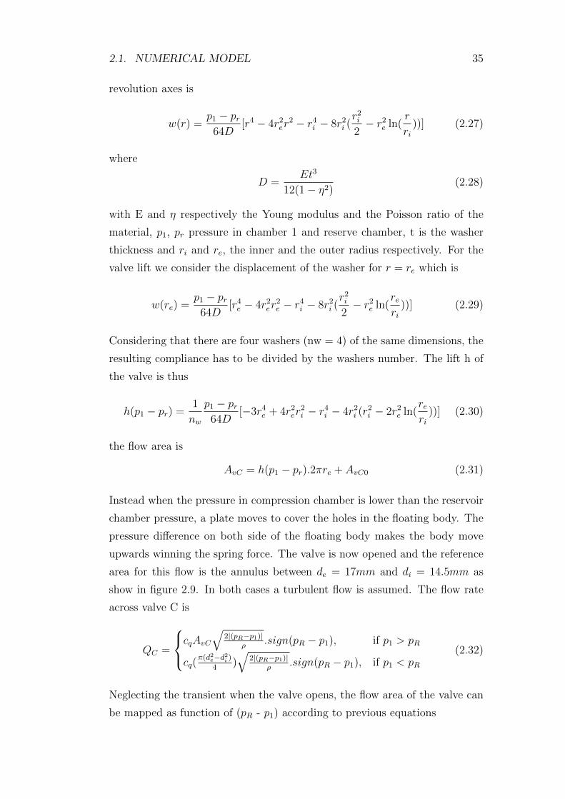
2.1. NUMERICAL MODEL 35
revolution axes is
w(r) =p1 − pr
64D[r4 − 4r2
er2 − r4
i − 8r2i (r2i
2− r2
e ln(r
ri))] (2.27)
where
D =Et3
12(1− η2)(2.28)
with E and η respectively the Young modulus and the Poisson ratio of the
material, p1, pr pressure in chamber 1 and reserve chamber, t is the washer
thickness and ri and re, the inner and the outer radius respectively. For the
valve lift we consider the displacement of the washer for r = re which is
w(re) =p1 − pr
64D[r4e − 4r2
er2e − r4
i − 8r2i (r2i
2− r2
e ln(reri
))] (2.29)
Considering that there are four washers (nw = 4) of the same dimensions, the
resulting compliance has to be divided by the washers number. The lift h of
the valve is thus
h(p1 − pr) =1
nw
p1 − pr64D
[−3r4e + 4r2
er2i − r4
i − 4r2i (r
2i − 2r2
e ln(reri
))] (2.30)
the flow area is
AvC = h(p1 − pr).2πre + AvC0 (2.31)
Instead when the pressure in compression chamber is lower than the reservoir
chamber pressure, a plate moves to cover the holes in the floating body. The
pressure difference on both side of the floating body makes the body move
upwards winning the spring force. The valve is now opened and the reference
area for this flow is the annulus between de = 17mm and di = 14.5mm as
show in figure 2.9. In both cases a turbulent flow is assumed. The flow rate
across valve C is
QC =
cqAvC√
2|(pR−p1)|ρ
.sign(pR − p1), if p1 > pR
cq(π(d2e−d2i )
4)√
2|(pR−p1)|ρ
.sign(pR − p1), if p1 < pR(2.32)
Neglecting the transient when the valve opens, the flow area of the valve can
be mapped as function of (pR - p1) according to previous equations
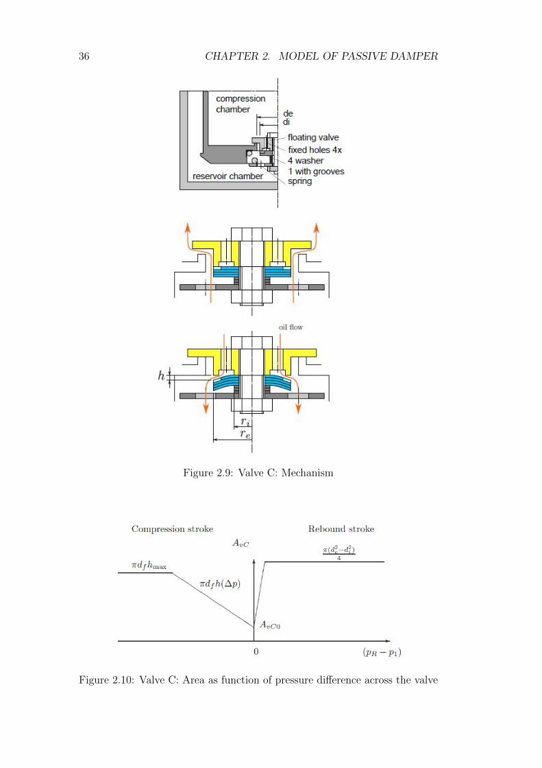
36 CHAPTER 2. MODEL OF PASSIVE DAMPER
Figure 2.9: Valve C: Mechanism
Figure 2.10: Valve C: Area as function of pressure difference across the valve

2.2. EXPERIMENT 37
2.2 Experiment
In this section we discuss about the experimental setup we use for physical
testing of our numerical model. The main aim of the physical testing are as
follows:-
1. Characterization of the passive hydrualic damper.
2. Validation of the numerical model.
2.2.1 Experimental Setup
For our study we use a hydraulic damper of secondary suspension system of
a train which is mounted on a rigid support and given excitation through a
hydraulic actuator. The experimental setup is shown in the figure below:-
Figure 2.11: Experimental setup for passive damper
The main components of the system are:-
38 CHAPTER 2. MODEL OF PASSIVE DAMPER
• A computer controlled hydraulic actuator.
• A hydraulic damper
• Position measurement system with Lasers
• Load cell for Force measurement.
• Pressure hoses
• Connecting cables
The description of the equipments used is given in the Table 2.1:
Table 2.1: Experimental setup for passive damper
The hydraulic actuator can be used to give different types of input
excitations like sinusoidal, ramp, sweep or random profile. The 2 lasers provide
the displacement measurement and a load cell at the base provides the value
of Force applied.
2.2.2 Experimental tests
Characterization test
For characterization of the passive damper, a sweep input with frequency from
1 Hz - 10 Hz is applied with different values of amplitude and the equivalent
damping and stiffness of the damper are calculated at different frequencies.
2.2. EXPERIMENT 39
From the Force data, displacement of the piston and frequency of the input
signal it is possible to estimate the equivalent stiffness and damping of the
hydraulic damper.
k =F
x(2.33)
r =1
ω(F
x) (2.34)
where,
F = Force on the piston
k = equivalent stiffness of the damper
r = equivalent damping of the damper
ω = frequency of the input
Fig 2.12 shows the stiffness and damping curves for hydraulic damper
in passive condition with external valve fully closed with sweep input (1Hz to
10Hz) and different amplitudes.
The stiffness and damping of a hydraulic damper depends on the
force required and amount of energy absorbed during flowing of viscous fluid
though the valve on piston from one chamber to another. From the graphs we
can make the following inferences about the characteristics of the hydraulic
damper.
1. The stiffness of the hydraulic damper at a constant amplitude increases
with frequency as the oil has less time to pass from one chamber to
another and compressibility of the fluid comes into effect, therefore the
net force exerted on piston increases.
2. The damping of the hydraulic damper decreases with increase in fre-
quency at constant amplitude for the same reason as less amount of
fluid actually moves through the valve, the compression of fluid is like
a spring phenomenon so less dissipation of energy, hence lower value of
damping.
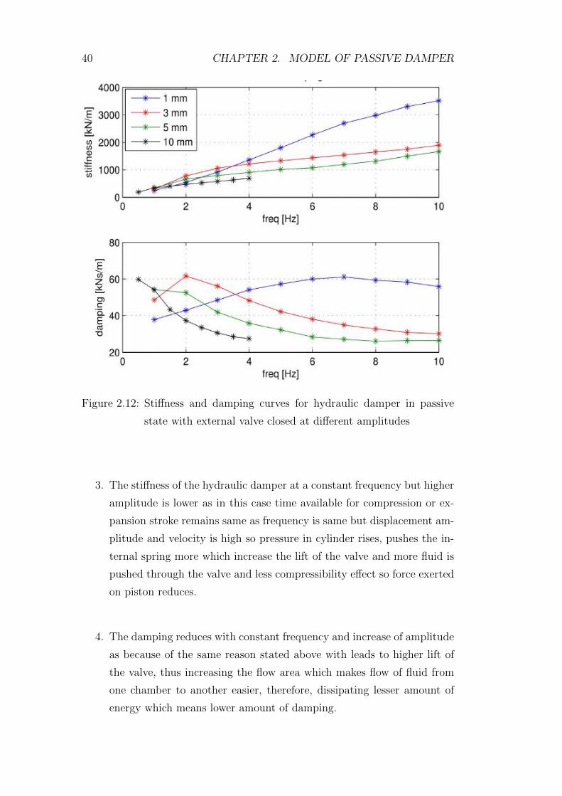
40 CHAPTER 2. MODEL OF PASSIVE DAMPER
Figure 2.12: Stiffness and damping curves for hydraulic damper in passive
state with external valve closed at different amplitudes
3. The stiffness of the hydraulic damper at a constant frequency but higher
amplitude is lower as in this case time available for compression or ex-
pansion stroke remains same as frequency is same but displacement am-
plitude and velocity is high so pressure in cylinder rises, pushes the in-
ternal spring more which increase the lift of the valve and more fluid is
pushed through the valve and less compressibility effect so force exerted
on piston reduces.
4. The damping reduces with constant frequency and increase of amplitude
as because of the same reason stated above with leads to higher lift of
the valve, thus increasing the flow area which makes flow of fluid from
one chamber to another easier, therefore, dissipating lesser amount of
energy which means lower amount of damping.
2.2. EXPERIMENT 41
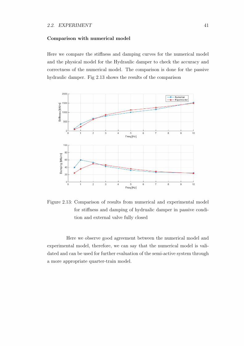
Comparison with numerical model
Here we compare the stiffness and damping curves for the numerical model
and the physical model for the Hydraulic damper to check the accuracy and
correctness of the numerical model. The comparison is done for the passive
hydraulic damper. Fig 2.13 shows the results of the comparison
Figure 2.13: Comparison of results from numerical and experimental model
for stiffness and damping of hydrualic damper in passive condi-
tion and external valve fully closed
Here we observe good agreement between the numerical model and
experimental model, therefore, we can say that the numerical model is vali-
dated and can be used for further evaluation of the semi-active system through
a more appropriate quarter-train model.
42 CHAPTER 2. MODEL OF PASSIVE DAMPER

Chapter 3
Development of the
Semi-Active Damper
Based on our discussion in the chapter ”State of the Art”, about various
types of Active/ Semi-Active solutions available for our application and also
from their relative advantages and disadvantages, we decided to use a Semi-
Active control system for our study. The main reason for this choice is that
for this application for which we are designing such a system, a semi-active
suspension offers a more cost effective, reliable and relatively less complex
solution. An active system such as a hydraulic or an electromagnetic system
is usually expensive and requires large modification in original component for
implementation, therefore for our purpose of study, a semi-active suspension
is a suitable choice.
In this chapter, we discuss the implementation method of Semi-
Active control in the numerical model of the passive hydraulic damper. As
described earlier, a semi active suspensions have similar components like a
passive damper i.e a spring and a damper, however the difference is that here
the properties of the damper can be varied. For this purpose, we have the
available options of magneto rheological damper or using a solenoid valve
or other external valve arrangement which could be controlled by our con-
trol strategies. Considering the cost effectiveness and amount of modification
required during manufacturing of the physical prototype at later stage, we
decide to introduce an external valve arrangement for varying the properties
43
44 CHAPTER 3. DEVELOPMENT OF THE SEMI-ACTIVE DAMPER
of the damper.
3.1 Numerical Model
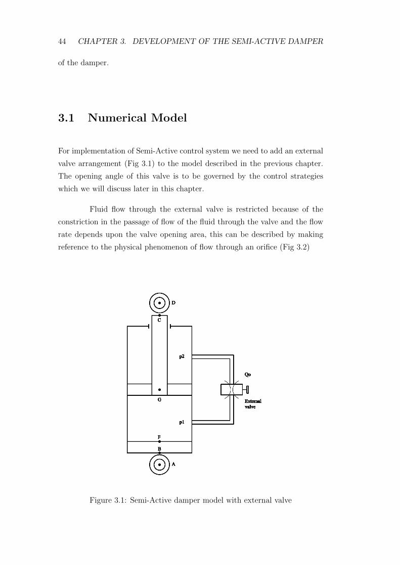
For implementation of Semi-Active control system we need to add an external
valve arrangement (Fig 3.1) to the model described in the previous chapter.
The opening angle of this valve is to be governed by the control strategies
which we will discuss later in this chapter.
Fluid flow through the external valve is restricted because of the
constriction in the passage of flow of the fluid through the valve and the flow
rate depends upon the valve opening area, this can be described by making
reference to the physical phenomenon of flow through an orifice (Fig 3.2)
Figure 3.1: Semi-Active damper model with external valve

3.1. NUMERICAL MODEL 45
Figure 3.2: Flow through orifice
where,
A0 is the area of the orifice
A2 is the minimum flow area = vena contracta
The fluid particles are accelerated between section 1 and 2.
Applying the continuity equation for the incompressible flow:
A1u1 = A2u2 = A3u3 (3.1)
A2 = CcA0 (3.2)
Cc is the contraction coefficient
Applying Bernoulli’s equation:
1
2ρu2
2 + p2 =1
2ρu2
1 + p1 (3.3)
where,
ρ is the density of the viscous fluid of the damper
p1, p2 are pressures in chamber 1 and 2.
u1, u2 are velocity of fluid at section 1 and 2
46 CHAPTER 3. DEVELOPMENT OF THE SEMI-ACTIVE DAMPER
Assuming that there is no pressure recovery during the expansion from
section 2 to section 3.
∆p = p1 − p2 = p1 − p3 (3.4)
p1 − p2 = ∆p =1
2ρ(u2
2 − u21) =
1
2ρ(1− (
A2
A1
)2)u22 (3.5)
⇒ u2 =
√2∆pρ√
1− (A2
A1)2
(3.6)
Volumetric flow rate QD (evaluated in minimum flow area):
QD = CcA0u2 =CcA0√
1− (A2
A1)2
√2∆p
ρ= CdA0
√2∆p
ρ(3.7)
where,
Cd =Cc√
1− C2c (A2
A1)2
⇒ Discharge coefficient (3.8)
The control strategy varies this valve area i.e A0 through an actuator to vary
the flow rate QD through the valve, thus, altering the damper characteris-
tics. To effectively study the effect of this Semi-Active damper on vibration
characteristics in a train, this numerical model is used in the model of a
Quarter-Train, described in the next section.

3.2. QUARTER-TRAIN MODEL REPRESENTATION 47
3.2 Quarter-Train Model Representation
Figure 3.3: Quarter Model of a Train
The simplest representation of a train suspension is a 2 DOF quarter-train
model with a secondary spring and damper connecting the chassis to the
bogie, which is in turn connected to the wheel by primary spring and damper,
as shown in Fig. 3.3. The mass representing the wheel, brakes and part of
the suspension linkage mass, is referred to as the unsprung mass. In order to
isolate the vehicle from irregularities of the track, the suspension is required to
act as a filter. However, while acting as a filter it is also required to carry the
static load of the vehicle. This creates a static deflection in the spring which
has to be taken into account in the suspension design. It is also required to
accommodate changes which occur in the static deflection due to changes in
load, unless some form of leveling mechanism is employed.
The quarter train model shown in Fig. 3.3 can be described by a
48 CHAPTER 3. DEVELOPMENT OF THE SEMI-ACTIVE DAMPER
pair of second-order differential equations:
MbZA + (r1 + r2)ZA − r2ZD + (K1 +K2)ZA −K2ZD = r1˙ZW +K1ZW (3.9)
McZD − r2ZA = r2ZD −K2ZA +K2ZD = 0 (3.10)
In a typical modern train, With moderate damping rates there are two distinct
modes of vibration, a chassis mode around 1 Hz and a bogie mode around 8
Hz. A fortuitous side effect of these ratios is that the single passive damper
imparts similar damping ratios to each of the modes.
3.3 Design of Control Strategy
In this section, we deal with the problem of designing a control law for semi
active suspension systems. A semi active suspension also consists of a spring
and a damper, but unlike a passive suspension, its characteristics can be
varied, governed by a suitable control strategy designed to obtain the desired
performance.
The most common control strategy used in industry for improving
ride quality is the conventional Skyhook control strategy, which has been
described in detail in the Chapter 1. For our study, we used Skyhook control
strategy as a reference to compare and evaluate the other 4 control logics
designed namely: Frequency based control on body acceleration, Frequency
based control on chassis velocity, Force Amplitude control loop and Force
control loop with fixed reference. In the next section, we discuss each of these
control strategies in detail.
3.4 Control Strategies studied
3.4.1 Frequency based control on Chassis Acceleration
This is a feedback loop control strategy. The aim of this strategy is to imple-
ment a frequency based control on the most critical parameter affecting ride
3.4. CONTROL STRATEGIES STUDIED 49
comfort i.e. the acceleration of the chassis. The intention is to determine the
frequency of acceleration on the chassis and calculate suitable opening angle
of the external valve, such that we can obtain maximum damping rate at
the first mode of resonance i.e 1 Hz, we also want to reduce the transmitted
vibrations to the chassis at higher frequencies to ultimately reduce the rms
acceleration on the chassis.
Therefore, we measure chassis acceleration as an input, which is then
filtered to compute Fourier transform to obtain a spectrum. This spectrum is
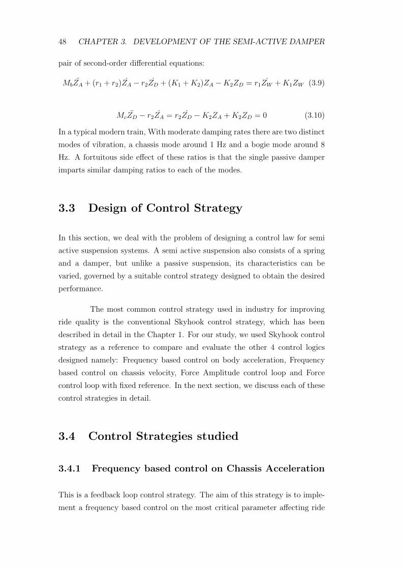
multiplied by a window as shown in Fig. 3.4, which gives high weighting to
frequencies in the range 0.5 - 3 Hz. The purpose of this window is to avoid
opening the external valve at frequencies close to first resonance mode i.e 1
Hz. This is required in order to have high value of equivalent damping at
these frequencies, as opening of external valve leads to reduction in equivalent
damping, which results in higher vibration amplitude at resonance and hence
reducing the ride comfort. For the same purpose, a condition is added in
the target law to keep the valve closed if the measured frequency of input
excitation is less than 2hz.
Figure 3.4: Frequency weighting window
The weighted spectrum obtained after multiplication with this win-
dow is then required to be further processed to give a unique value of frequency.
For this purpose, we pick all the peaks of the spectrum above a threshold
value, which has to be suitably assigned. If the threshold is set too high, we
might miss important components of frequency, and on the other hand, if it
is too low, the resulting data will contain considerable noise and other non-
significant components. Therefore, for our study we used a threshold value of
0.4Amax, where Amax, is the peak amplitude of the spectrum.
50 CHAPTER 3. DEVELOPMENT OF THE SEMI-ACTIVE DAMPER
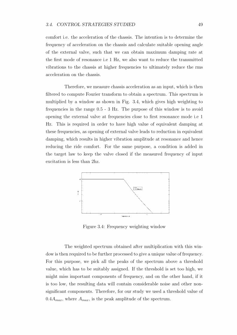
The frequency peaks, whose amplitudes are higher than threshold
are then average weighted on their amplitudes to obtain a unique value of
frequency, which can also be termed as equivalent frequency.
feq =n∑i=1
AifiAi
(3.11)
where,
n = number of peaks with amplitude above the threshold
Then this equivalent frequency is used to find out the suitable valve
opening angle, through the target correlation curve between measured fre-
quency of input and valve opening angle (explained in details in next section).
The complete schematic of the control strategy is shown in fig 3.5.
Figure 3.5: Control loop for control on Chassis Acceleration
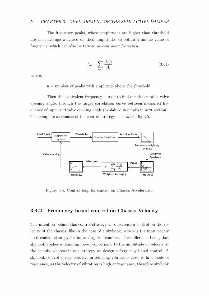
3.4.2 Frequency based control on Chassis Velocity
The intention behind this control strategy is to exercise a control on the ve-
locity of the chassis, like in the case of a skyhook, which is the most widely
used control strategy for improving ride comfort. The difference being that
skyhook applies a damping force proportional to the amplitude of velocity at
the chassis, whereas in our strategy we design a frequency based control. A
skyhook control is very effective in reducing vibrations close to first mode of
resonance, as the velocity of vibration is high at resonance, therefore skyhook
3.4. CONTROL STRATEGIES STUDIED 51
tries to offer maximum damping, but at high frequency excitations, even at
moderate amplitudes, the measured velocity of vibration remains high and
therefore skyhook tries to offer high damping by having lower opening angle
of external valve, which is exactly opposite to our requirement as we have dis-
cussed earlier that because of the changes in damper characteristics at high
frequencies, we need to open the valve to reduce transmissibility. We try to
counter this problem by having a frequency based control on velocity, so we
can have higher damping near resonance and can reduce transmissibility at
high frequency.
The control algorithm is the same like the previous case, only differ-
ence is that instead of measuring acceleration, here we measure velocity of the
chassis as an input. Which is then used to calculate the frequency and hence
the valve opening angle. Fig. 3.6
Figure 3.6: Control loop for control on Chassis Velocity
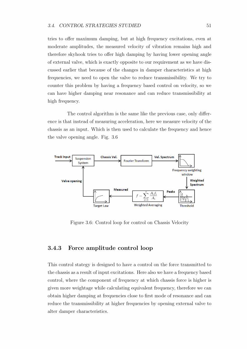
3.4.3 Force amplitude control loop
This control stategy is designed to have a control on the force transmitted to
the chassis as a result of input excitations. Here also we have a frequency based
control, where the component of frequency at which chassis force is higher is
given more weightage while calculating equivalent frequency, therefore we can
obtain higher damping at frequencies close to first mode of resonance and can
reduce the transmissibility at higher frequencies by opening external valve to
alter damper characteristics.
52 CHAPTER 3. DEVELOPMENT OF THE SEMI-ACTIVE DAMPER
The control algorithm takes Force on the chassis as an input, which
in turn is used to compute frequency by the method used in previous case and
hence we obtain the required value of valve opening angle through the target
curve. Fig. 3.7
Figure 3.7: Control loop for control on Body Force
3.4.4 Force control with fixed reference
This control strategy is based on Amplitude of chassis force, insead of the
frequency. The force transmitted to the chassis will have significant effect on
the ride comfort, therefore, in this strategy we simply try to reduce the chassis
force by varying the characteristics of the damper.
In the control algorithm, we again measure the Force on chassis as
an input, Fig 3.8, then we do the Fourier transform of the signal and multiply
with a frequency weighting window as described in earlier control strategies,
but after that instead of selecting peaks and doing weighted average, we obtain
RMS value of the force from the following formula :-
Frms =
√∫ fm
0
P (f)dF (3.12)
where,
Frms is the RMS Force
P(f) is the power spectral density function
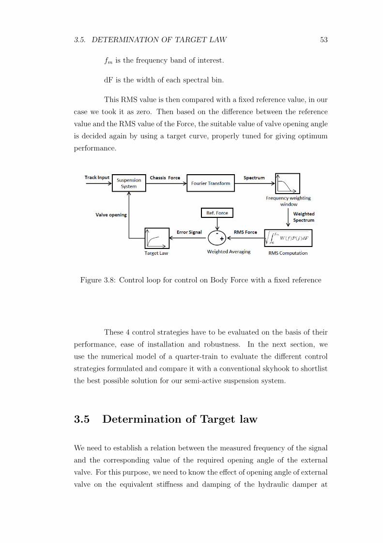
3.5. DETERMINATION OF TARGET LAW 53
fm is the frequency band of interest.
dF is the width of each spectral bin.
This RMS value is then compared with a fixed reference value, in our
case we took it as zero. Then based on the difference between the reference
value and the RMS value of the Force, the suitable value of valve opening angle
is decided again by using a target curve, properly tuned for giving optimum
performance.
Figure 3.8: Control loop for control on Body Force with a fixed reference
These 4 control strategies have to be evaluated on the basis of their
performance, ease of installation and robustness. In the next section, we
use the numerical model of a quarter-train to evaluate the different control
strategies formulated and compare it with a conventional skyhook to shortlist
the best possible solution for our semi-active suspension system.
3.5 Determination of Target law
We need to establish a relation between the measured frequency of the signal
and the corresponding value of the required opening angle of the external
valve. For this purpose, we need to know the effect of opening angle of external
valve on the equivalent stiffness and damping of the hydraulic damper at
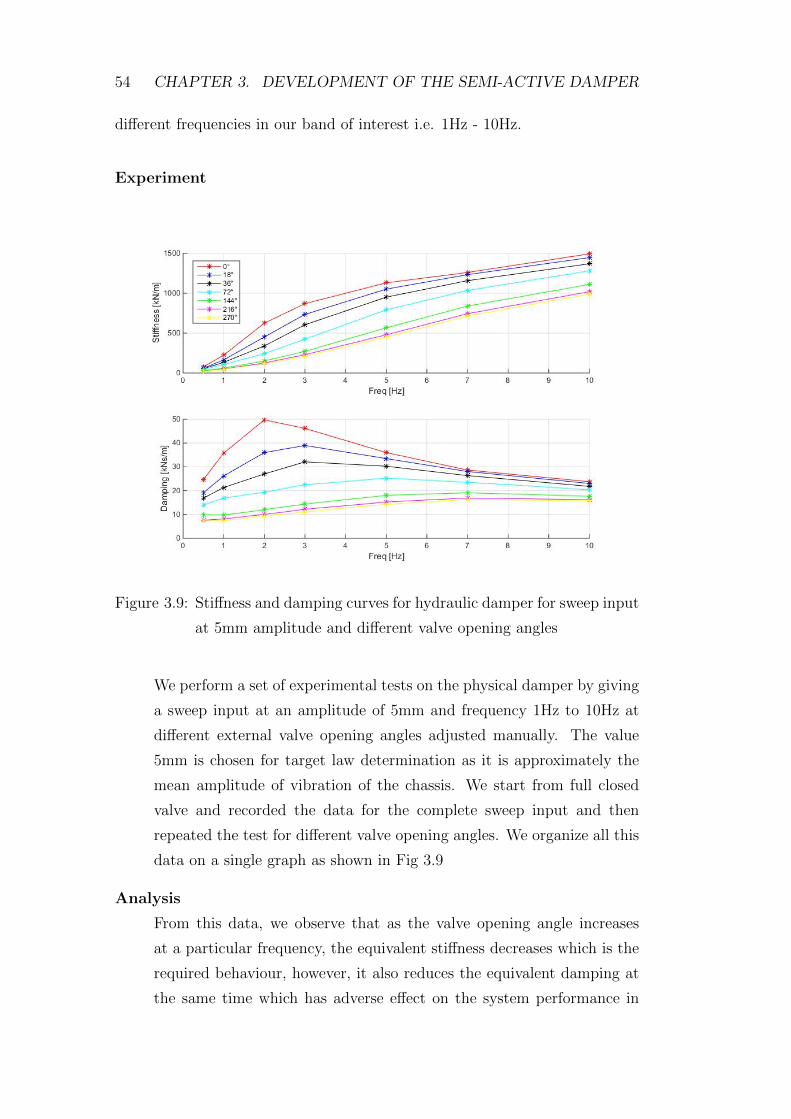
54 CHAPTER 3. DEVELOPMENT OF THE SEMI-ACTIVE DAMPER
different frequencies in our band of interest i.e. 1Hz - 10Hz.
Experiment
Figure 3.9: Stiffness and damping curves for hydraulic damper for sweep input
at 5mm amplitude and different valve opening angles
We perform a set of experimental tests on the physical damper by giving
a sweep input at an amplitude of 5mm and frequency 1Hz to 10Hz at
different external valve opening angles adjusted manually. The value
5mm is chosen for target law determination as it is approximately the
mean amplitude of vibration of the chassis. We start from full closed
valve and recorded the data for the complete sweep input and then
repeated the test for different valve opening angles. We organize all this
data on a single graph as shown in Fig 3.9
Analysis
From this data, we observe that as the valve opening angle increases
at a particular frequency, the equivalent stiffness decreases which is the
required behaviour, however, it also reduces the equivalent damping at
the same time which has adverse effect on the system performance in
3.5. DETERMINATION OF TARGET LAW 55
the frequency range close to the natural frequency of the system, as we
need higher damping to control the vibration amplitude at resonance.
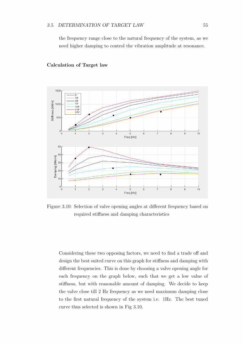
Calculation of Target law
Figure 3.10: Selection of valve opening angles at different frequency based on
required stiffness and damping characteristics
Considering these two opposing factors, we need to find a trade off and
design the best suited curve on this graph for stiffness and damping with
different frequencies. This is done by choosing a valve opening angle for
each frequency on the graph below, such that we get a low value of
stiffness, but with reasonable amount of damping. We decide to keep
the valve close till 2 Hz frequency as we need maximum damping close
to the first natural frequency of the system i.e. 1Hz. The best tuned
curve thus selected is shown in Fig 3.10.
56 CHAPTER 3. DEVELOPMENT OF THE SEMI-ACTIVE DAMPER
Frequency (Hz) Valve angle (degrees)
1 0
2 0
3 54
4 80
5 216
7 270
8 324
9.5 360
Table 3.1: Selected valve opening angles for different frequencies
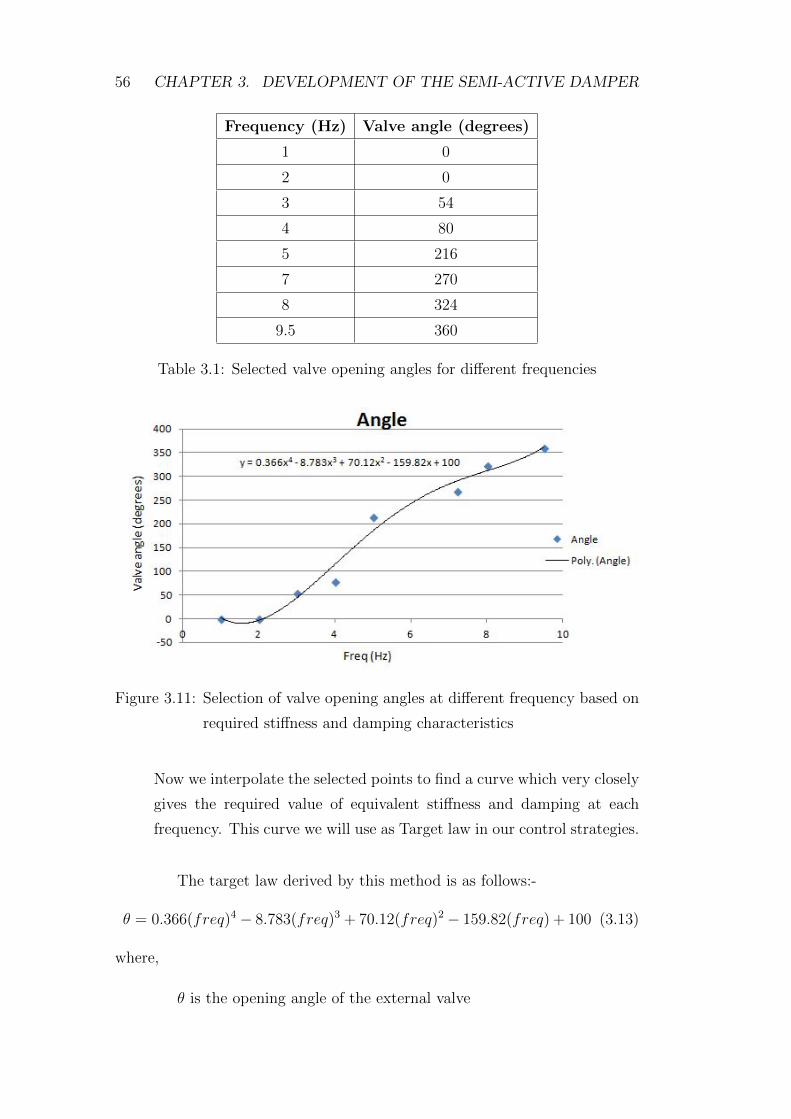
Figure 3.11: Selection of valve opening angles at different frequency based on
required stiffness and damping characteristics
Now we interpolate the selected points to find a curve which very closely
gives the required value of equivalent stiffness and damping at each
frequency. This curve we will use as Target law in our control strategies.
The target law derived by this method is as follows:-
θ = 0.366(freq)4 − 8.783(freq)3 + 70.12(freq)2 − 159.82(freq) + 100 (3.13)
where,
θ is the opening angle of the external valve
3.6. NUMERICAL TEST 57
freq is the measured frequency
3.6 Numerical Test
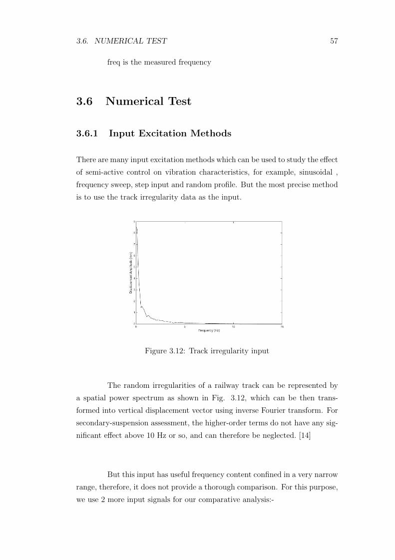
3.6.1 Input Excitation Methods
There are many input excitation methods which can be used to study the effect
of semi-active control on vibration characteristics, for example, sinusoidal ,
frequency sweep, step input and random profile. But the most precise method
is to use the track irregularity data as the input.
Figure 3.12: Track irregularity input
The random irregularities of a railway track can be represented by
a spatial power spectrum as shown in Fig. 3.12, which can be then trans-
formed into vertical displacement vector using inverse Fourier transform. For
secondary-suspension assessment, the higher-order terms do not have any sig-
nificant effect above 10 Hz or so, and can therefore be neglected. [14]
But this input has useful frequency content confined in a very narrow
range, therefore, it does not provide a thorough comparison. For this purpose,
we use 2 more input signals for our comparative analysis:-
58 CHAPTER 3. DEVELOPMENT OF THE SEMI-ACTIVE DAMPER
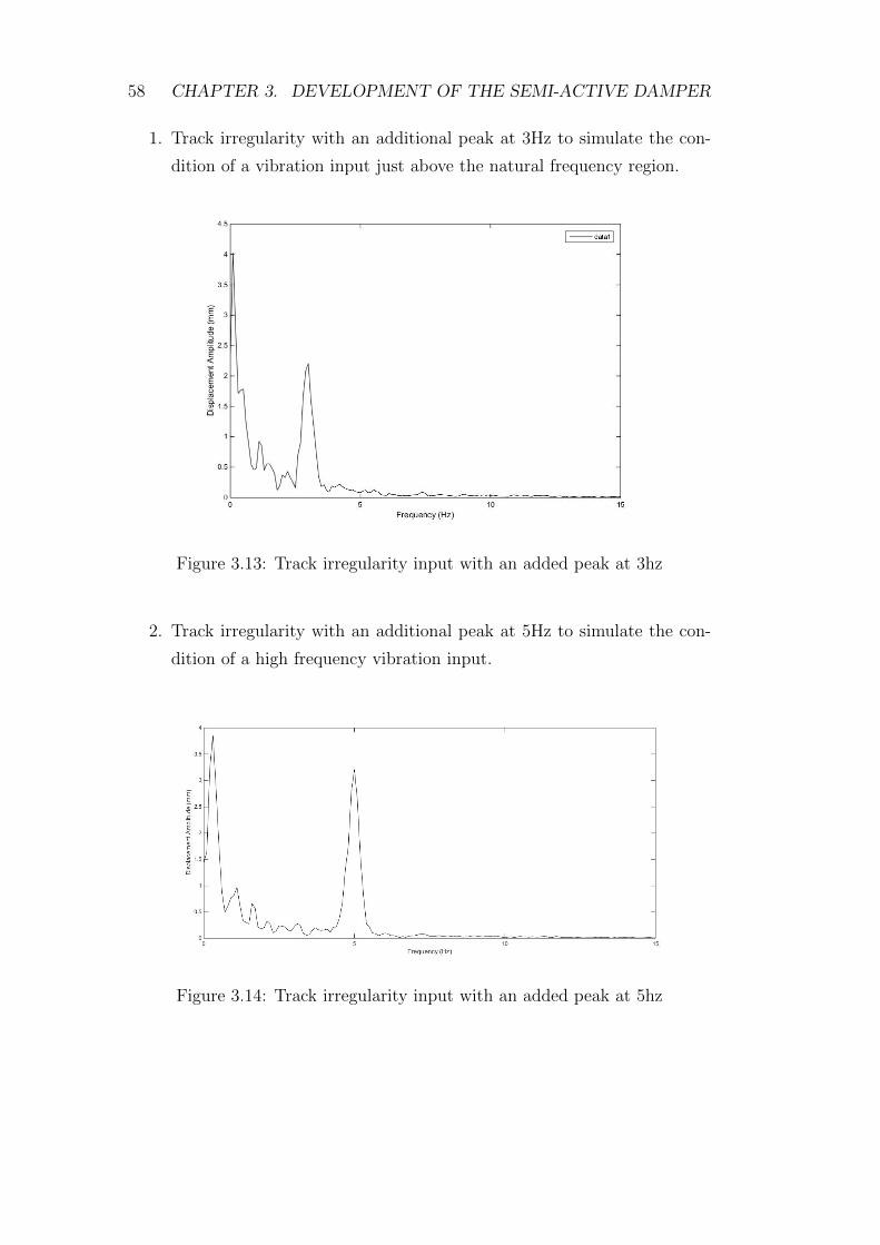
1. Track irregularity with an additional peak at 3Hz to simulate the con-
dition of a vibration input just above the natural frequency region.
Figure 3.13: Track irregularity input with an added peak at 3hz
2. Track irregularity with an additional peak at 5Hz to simulate the con-
dition of a high frequency vibration input.
Figure 3.14: Track irregularity input with an added peak at 5hz
3.6. NUMERICAL TEST 59
3.6.2 Results
In order to compare the performance of the control strategies with respect to
conventional Skyhook control and to shortlist the optimum one, we performed
numerical simulation on all control strategies and also on skyhook and passive
system. The simulations are done for 3 input excitation types described above.
The results are recorded and compared for the following parameters:-
1. RMS Acceleration
2. RMS Velocity
3. RMS Displacement
4. Peak Acceleration
5. Peak Velocity
6. Peak Displacement
All the recorded values are then normalized by the values for passive damper
so that we can notice the improvement or deterioration with respect to the
passive condition. We also simulated the control strategies with and without
the frequency weighting window described in the previous section to observe
the effect of the window on the performance.
The results are summarized in the following tables and figures:
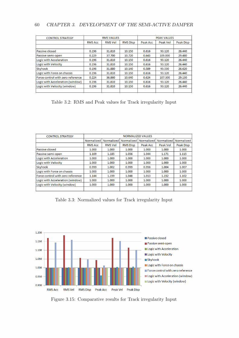
60 CHAPTER 3. DEVELOPMENT OF THE SEMI-ACTIVE DAMPER
Table 3.2: RMS and Peak values for Track irregularity Input
Table 3.3: Normalized values for Track irregularity Input
Figure 3.15: Comparative results for Track irregularity Input
3.6. NUMERICAL TEST 61
Observations
1. Since the frequency content of the input excitation is concentrated in
the narrow frequency band less than 2hz so the external valve remains
closed for our control strategies based on frequency measurement i.e.
logic on acceleration, velocity and force, so the results are similar to
passive condition.
2. For passive semi-open condition, the external valve is always half open,
therefore it offers lesser damping and as the signal is concentrated in
narrow frequency band close to first eigen mode of natural frequency,
therefore, resonance is more prominent due to less damping which is an
adverse effect.
3. Skyhook offers some improvement in peak acceleration as it is based on
velocity of chassis, which is higher in frequency range close to resonance
because of higher amplitude of vibration, therefore it offers maximum
damping.
4. For the control strategy on Chassis Force with zero reference, the exter-
nal valve opens as it senses a considerable amount of force at resonance,
again reducing the effective damping which is not as per the require-
ments.
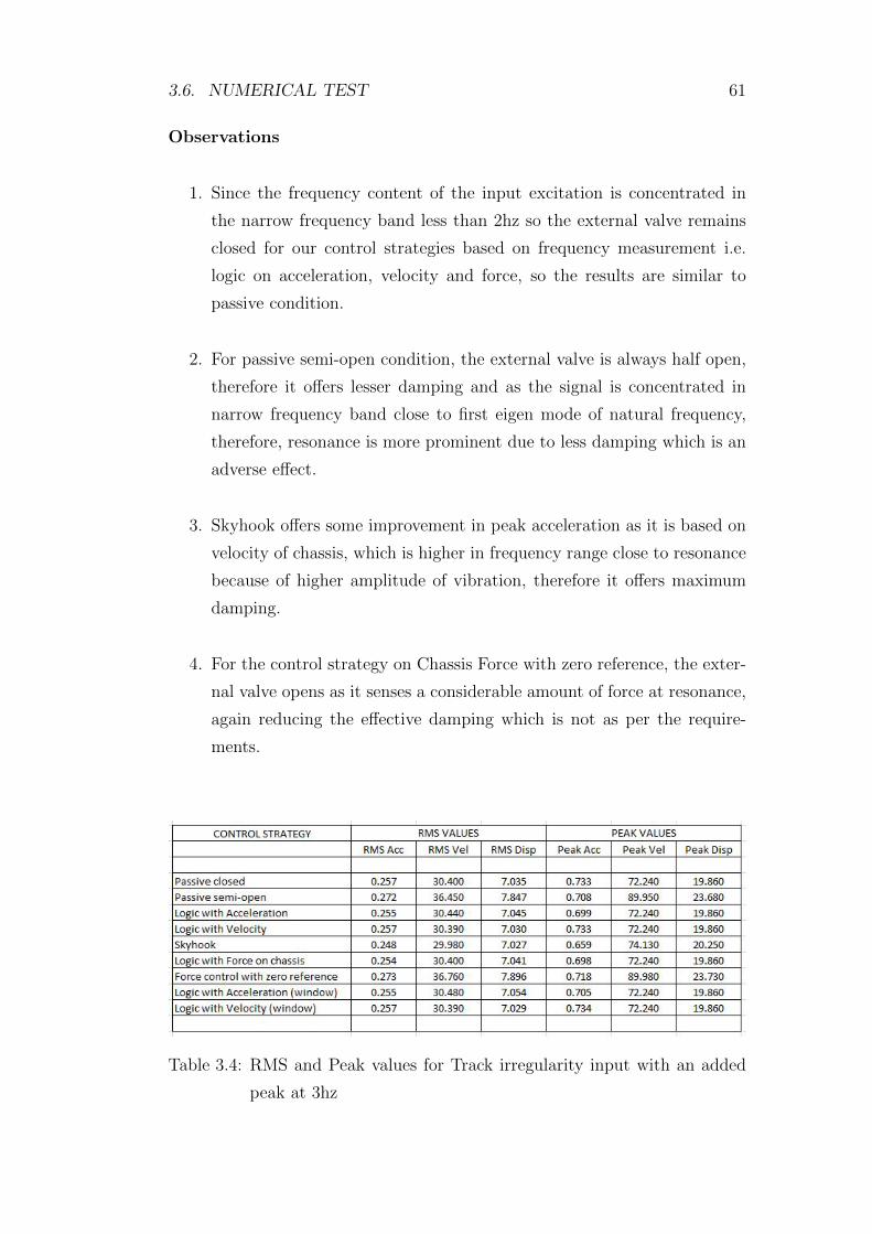
Table 3.4: RMS and Peak values for Track irregularity input with an added
peak at 3hz
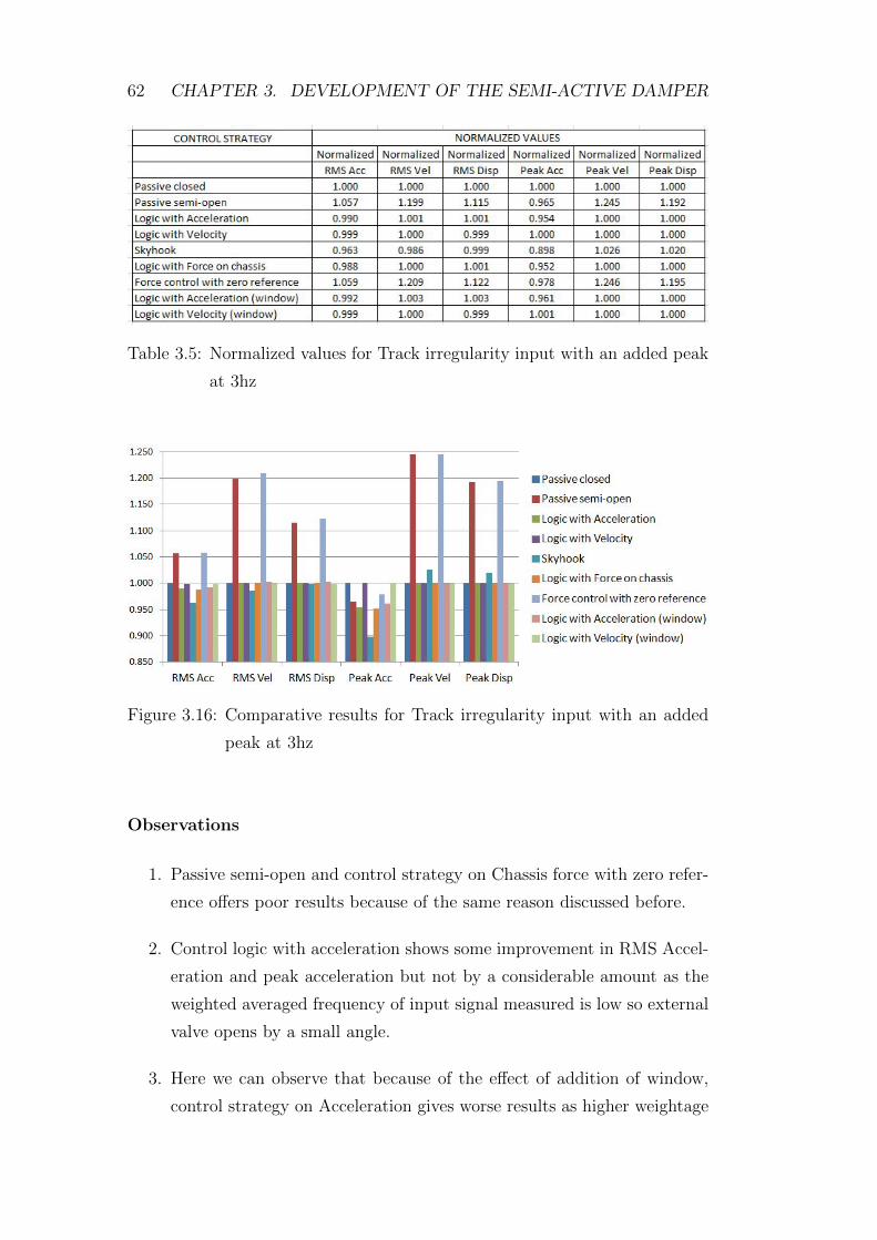
62 CHAPTER 3. DEVELOPMENT OF THE SEMI-ACTIVE DAMPER
Table 3.5: Normalized values for Track irregularity input with an added peak
at 3hz
Figure 3.16: Comparative results for Track irregularity input with an added
peak at 3hz
Observations
1. Passive semi-open and control strategy on Chassis force with zero refer-
ence offers poor results because of the same reason discussed before.
2. Control logic with acceleration shows some improvement in RMS Accel-
eration and peak acceleration but not by a considerable amount as the
weighted averaged frequency of input signal measured is low so external
valve opens by a small angle.
3. Here we can observe that because of the effect of addition of window,
control strategy on Acceleration gives worse results as higher weightage
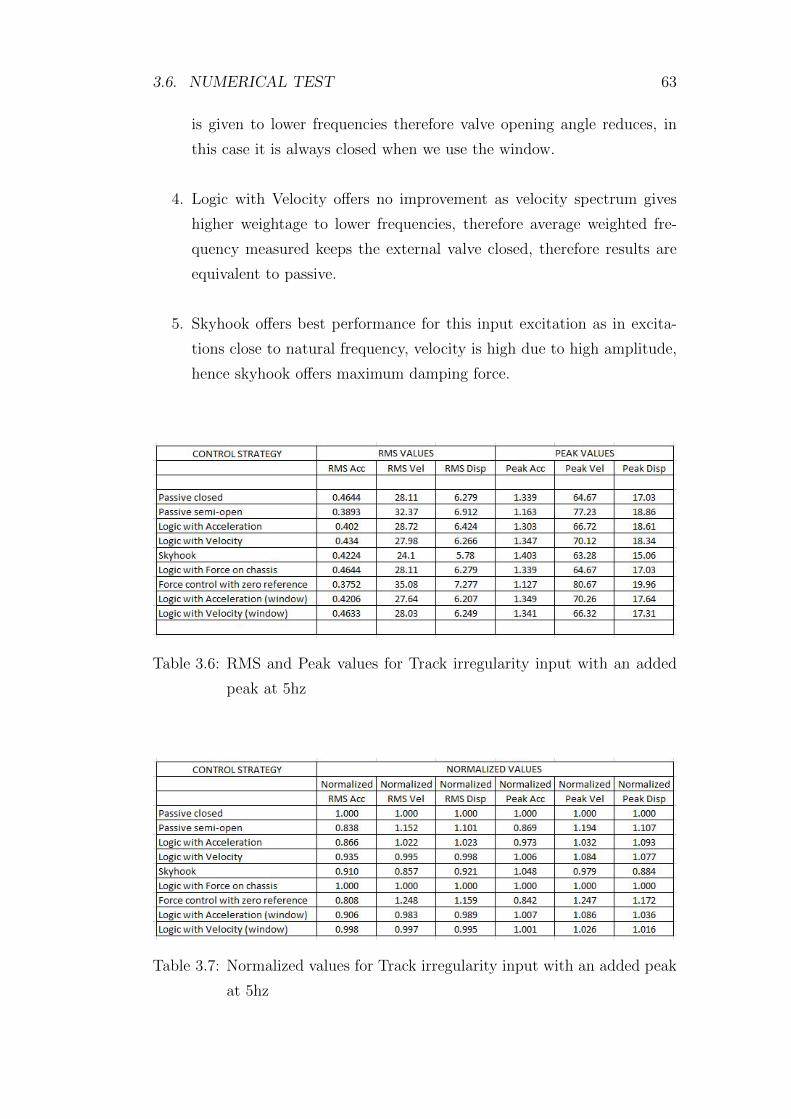
3.6. NUMERICAL TEST 63
is given to lower frequencies therefore valve opening angle reduces, in
this case it is always closed when we use the window.
4. Logic with Velocity offers no improvement as velocity spectrum gives
higher weightage to lower frequencies, therefore average weighted fre-
quency measured keeps the external valve closed, therefore results are
equivalent to passive.
5. Skyhook offers best performance for this input excitation as in excita-
tions close to natural frequency, velocity is high due to high amplitude,
hence skyhook offers maximum damping force.
Table 3.6: RMS and Peak values for Track irregularity input with an added
peak at 5hz
Table 3.7: Normalized values for Track irregularity input with an added peak
at 5hz
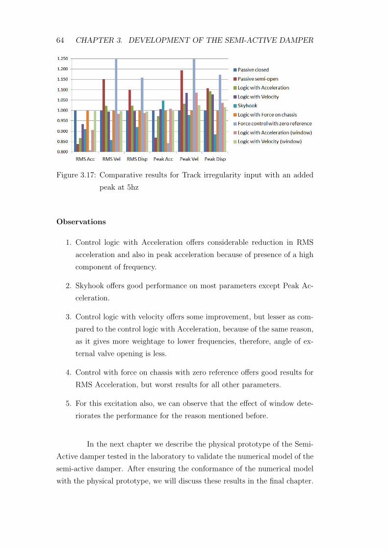
64 CHAPTER 3. DEVELOPMENT OF THE SEMI-ACTIVE DAMPER
Figure 3.17: Comparative results for Track irregularity input with an added
peak at 5hz
Observations
1. Control logic with Acceleration offers considerable reduction in RMS
acceleration and also in peak acceleration because of presence of a high
component of frequency.
2. Skyhook offers good performance on most parameters except Peak Ac-
celeration.
3. Control logic with velocity offers some improvement, but lesser as com-
pared to the control logic with Acceleration, because of the same reason,
as it gives more weightage to lower frequencies, therefore, angle of ex-
ternal valve opening is less.
4. Control with force on chassis with zero reference offers good results for
RMS Acceleration, but worst results for all other parameters.
5. For this excitation also, we can observe that the effect of window dete-
riorates the performance for the reason mentioned before.
In the next chapter we describe the physical prototype of the Semi-
Active damper tested in the laboratory to validate the numerical model of the
semi-active damper. After ensuring the conformance of the numerical model
with the physical prototype, we will discuss these results in the final chapter.
Chapter 4
Prototype of the Semi-Active
Damper
In this chapter we describe the prototype of the Semi-Active Hydraulic Damper
we created and tested in laboratory. The main aim of the physical testing are
as follows:-
1. Validation of the semi-active control action on the numerical model of
the single damper with experimental results.
2. Determination of a correlation between measured frequency and corre-
sponding value of required valve opening angle i.e. the target law.
3. To evaluate the working of the hardware components like sensors, ac-
tuators, electronic control unit and other electronic components and
connections required for the actual system.
4. To physically test and evaluate the proposed solution as a whole.
4.1 Semi-Active damper prototype
As we discussed in the previous chapter, for our study we decided to use a
semi-active control system with an external valve to vary the characteristics
of the hydraulic damper. For the actuator, we decide to use a servo motor
65
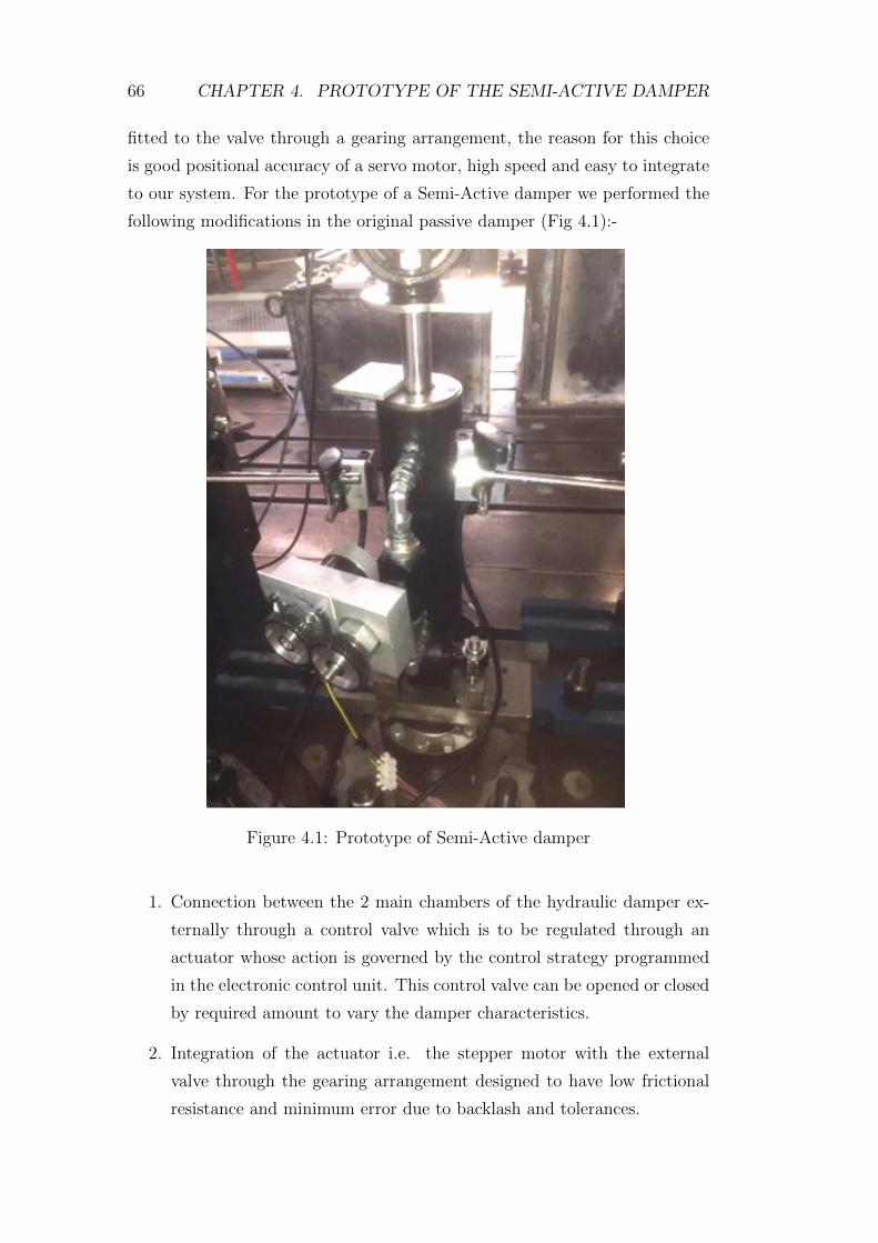
66 CHAPTER 4. PROTOTYPE OF THE SEMI-ACTIVE DAMPER
fitted to the valve through a gearing arrangement, the reason for this choice
is good positional accuracy of a servo motor, high speed and easy to integrate
to our system. For the prototype of a Semi-Active damper we performed the
following modifications in the original passive damper (Fig 4.1):-
Figure 4.1: Prototype of Semi-Active damper
1. Connection between the 2 main chambers of the hydraulic damper ex-
ternally through a control valve which is to be regulated through an
actuator whose action is governed by the control strategy programmed
in the electronic control unit. This control valve can be opened or closed
by required amount to vary the damper characteristics.
2. Integration of the actuator i.e. the stepper motor with the external
valve through the gearing arrangement designed to have low frictional
resistance and minimum error due to backlash and tolerances.
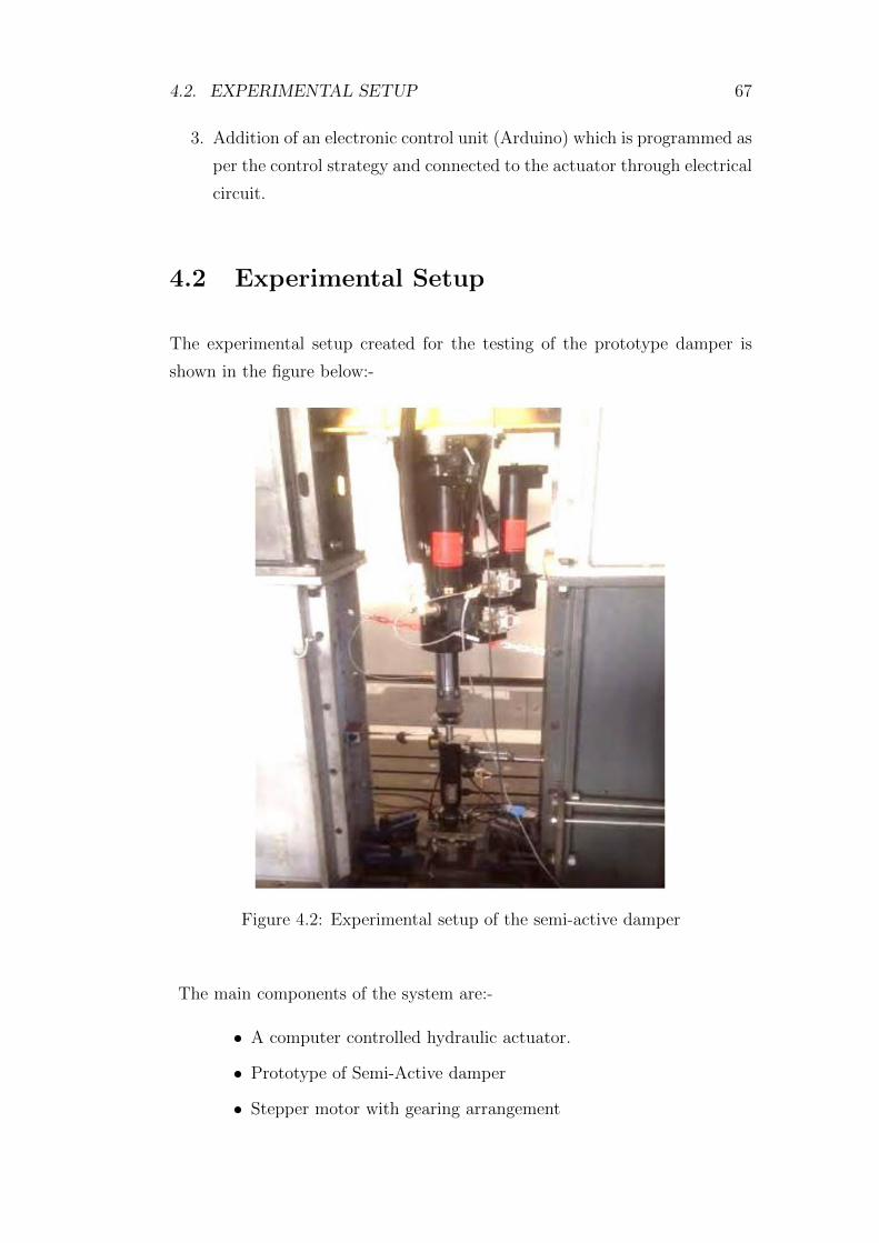
4.2. EXPERIMENTAL SETUP 67
3. Addition of an electronic control unit (Arduino) which is programmed as
per the control strategy and connected to the actuator through electrical
circuit.
4.2 Experimental Setup
The experimental setup created for the testing of the prototype damper is
shown in the figure below:-
Figure 4.2: Experimental setup of the semi-active damper
The main components of the system are:-
• A computer controlled hydraulic actuator.
• Prototype of Semi-Active damper
• Stepper motor with gearing arrangement
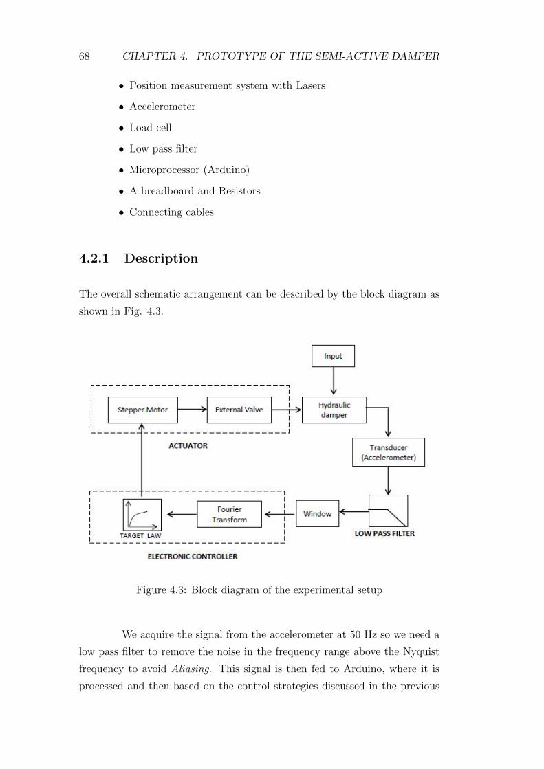
68 CHAPTER 4. PROTOTYPE OF THE SEMI-ACTIVE DAMPER
• Position measurement system with Lasers
• Accelerometer
• Load cell
• Low pass filter
• Microprocessor (Arduino)
• A breadboard and Resistors
• Connecting cables
4.2.1 Description
The overall schematic arrangement can be described by the block diagram as
shown in Fig. 4.3.
Figure 4.3: Block diagram of the experimental setup
We acquire the signal from the accelerometer at 50 Hz so we need a
low pass filter to remove the noise in the frequency range above the Nyquist
frequency to avoid Aliasing. This signal is then fed to Arduino, where it is
processed and then based on the control strategies discussed in the previous
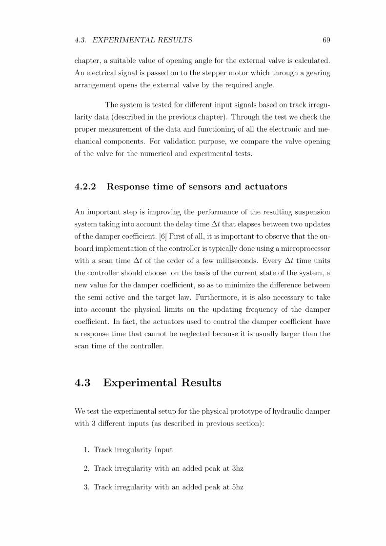
4.3. EXPERIMENTAL RESULTS 69
chapter, a suitable value of opening angle for the external valve is calculated.
An electrical signal is passed on to the stepper motor which through a gearing
arrangement opens the external valve by the required angle.
The system is tested for different input signals based on track irregu-
larity data (described in the previous chapter). Through the test we check the
proper measurement of the data and functioning of all the electronic and me-
chanical components. For validation purpose, we compare the valve opening
of the valve for the numerical and experimental tests.
4.2.2 Response time of sensors and actuators
An important step is improving the performance of the resulting suspension
system taking into account the delay time ∆t that elapses between two updates
of the damper coefficient. [6] First of all, it is important to observe that the on-
board implementation of the controller is typically done using a microprocessor
with a scan time ∆t of the order of a few milliseconds. Every ∆t time units
the controller should choose on the basis of the current state of the system, a
new value for the damper coefficient, so as to minimize the difference between
the semi active and the target law. Furthermore, it is also necessary to take
into account the physical limits on the updating frequency of the damper
coefficient. In fact, the actuators used to control the damper coefficient have
a response time that cannot be neglected because it is usually larger than the
scan time of the controller.
4.3 Experimental Results
We test the experimental setup for the physical prototype of hydraulic damper
with 3 different inputs (as described in previous section):
1. Track irregularity Input
2. Track irregularity with an added peak at 3hz
3. Track irregularity with an added peak at 5hz
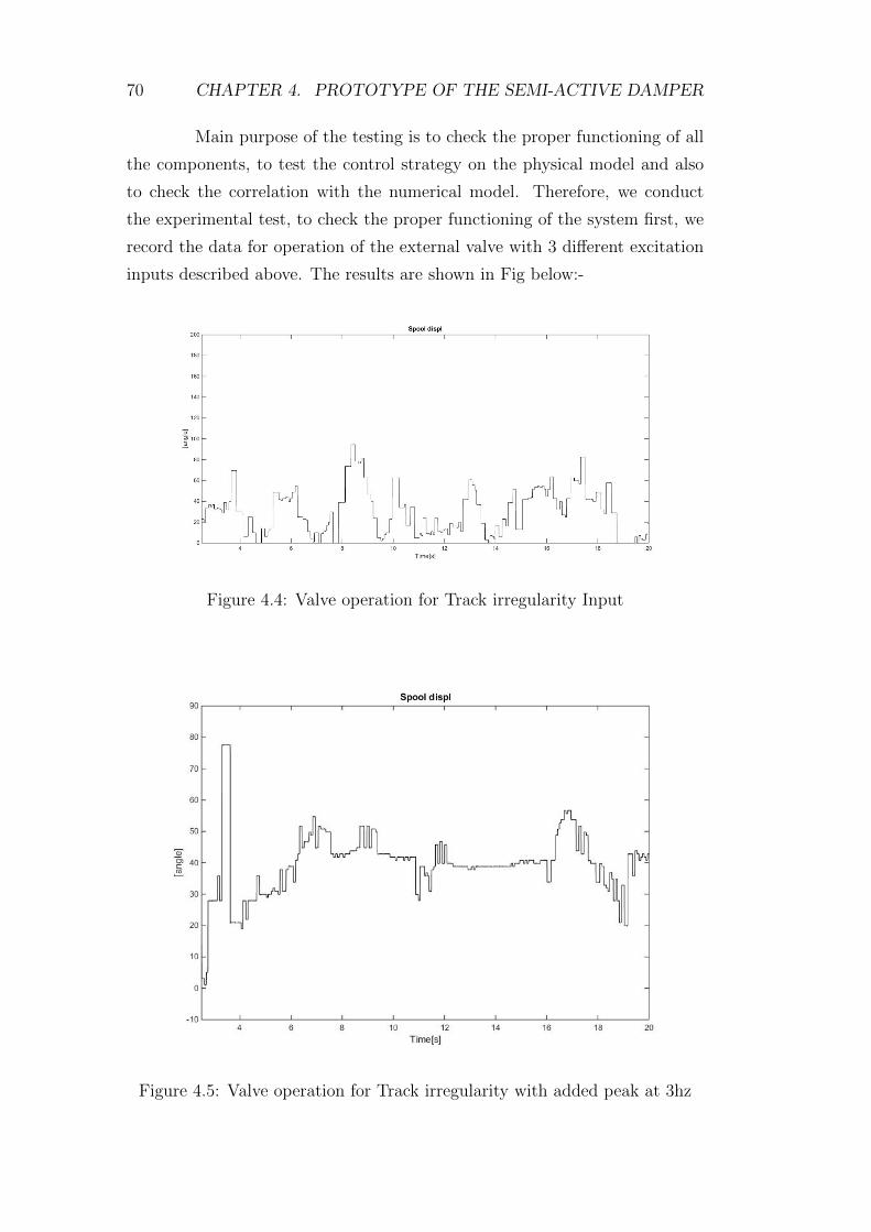
70 CHAPTER 4. PROTOTYPE OF THE SEMI-ACTIVE DAMPER
Main purpose of the testing is to check the proper functioning of all
the components, to test the control strategy on the physical model and also
to check the correlation with the numerical model. Therefore, we conduct
the experimental test, to check the proper functioning of the system first, we
record the data for operation of the external valve with 3 different excitation
inputs described above. The results are shown in Fig below:-
Figure 4.4: Valve operation for Track irregularity Input
Figure 4.5: Valve operation for Track irregularity with added peak at 3hz
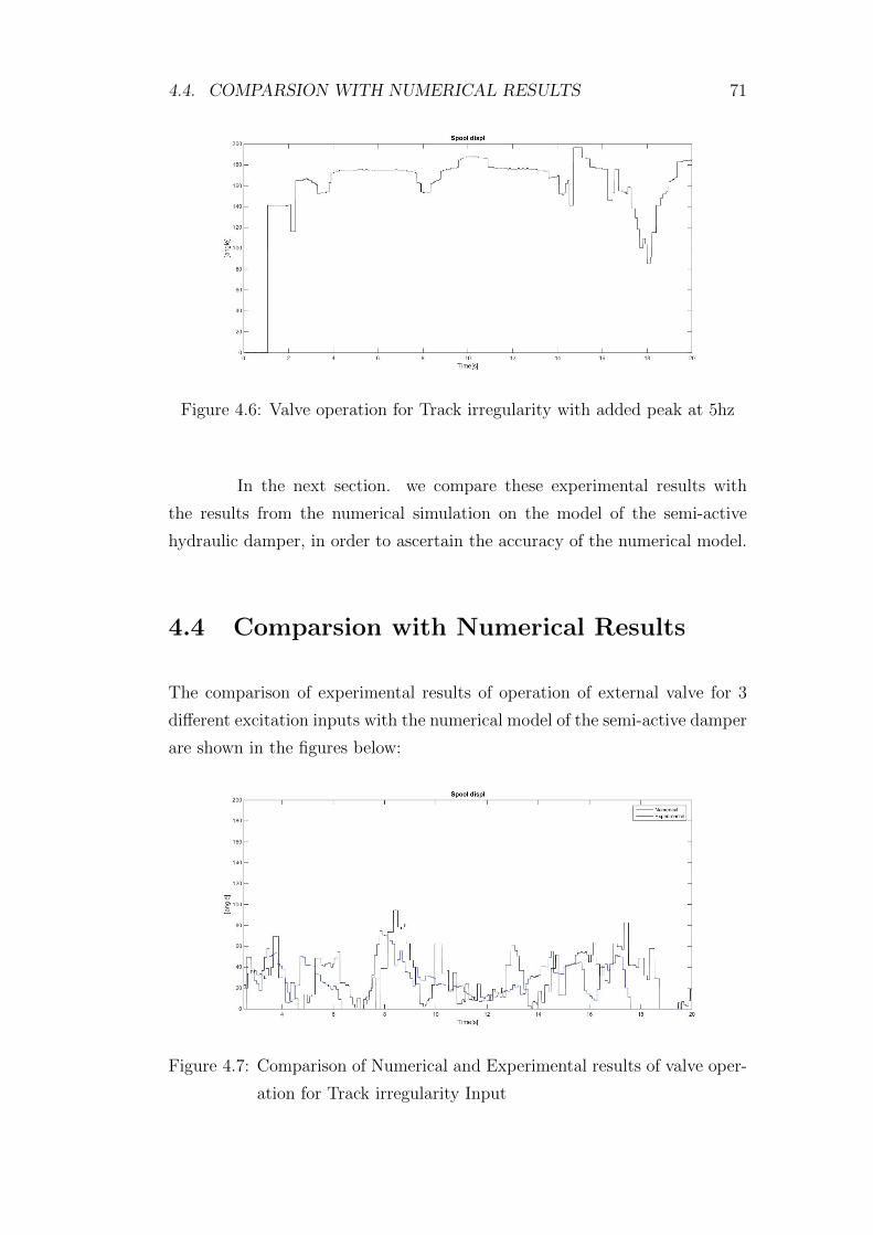
4.4. COMPARSION WITH NUMERICAL RESULTS 71
Figure 4.6: Valve operation for Track irregularity with added peak at 5hz
In the next section. we compare these experimental results with
the results from the numerical simulation on the model of the semi-active
hydraulic damper, in order to ascertain the accuracy of the numerical model.
4.4 Comparsion with Numerical Results
The comparison of experimental results of operation of external valve for 3
different excitation inputs with the numerical model of the semi-active damper
are shown in the figures below:
Figure 4.7: Comparison of Numerical and Experimental results of valve oper-
ation for Track irregularity Input
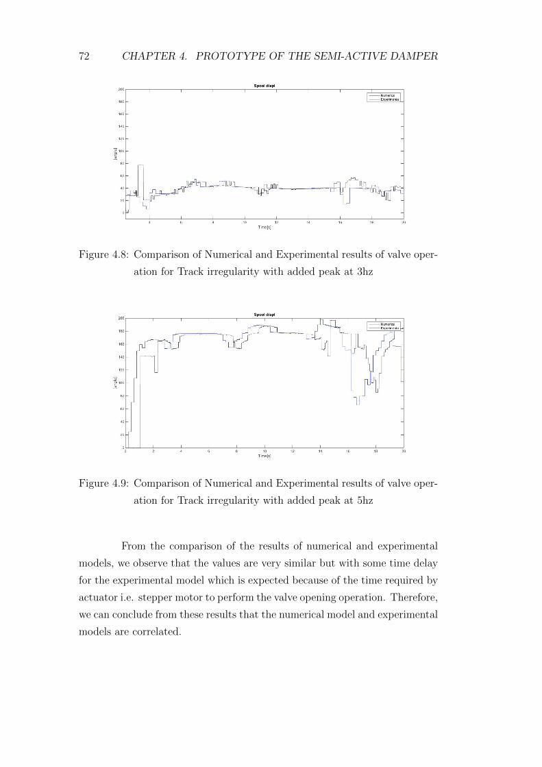
72 CHAPTER 4. PROTOTYPE OF THE SEMI-ACTIVE DAMPER
Figure 4.8: Comparison of Numerical and Experimental results of valve oper-
ation for Track irregularity with added peak at 3hz
Figure 4.9: Comparison of Numerical and Experimental results of valve oper-
ation for Track irregularity with added peak at 5hz
From the comparison of the results of numerical and experimental
models, we observe that the values are very similar but with some time delay
for the experimental model which is expected because of the time required by
actuator i.e. stepper motor to perform the valve opening operation. Therefore,
we can conclude from these results that the numerical model and experimental
models are correlated.
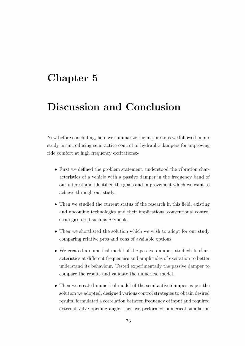
Chapter 5
Discussion and Conclusion
Now before concluding, here we summarize the major steps we followed in our
study on introducing semi-active control in hydraulic dampers for improving
ride comfort at high frequency excitations:-
• First we defined the problem statement, understood the vibration char-
acteristics of a vehicle with a passive damper in the frequency band of
our interest and identified the goals and improvement which we want to
achieve through our study.
• Then we studied the current status of the research in this field, existing
and upcoming technologies and their implications, conventional control
strategies used such as Skyhook.
• Then we shortlisted the solution which we wish to adopt for our study
comparing relative pros and cons of available options.
• We created a numerical model of the passive damper, studied its char-
acteristics at different frequencies and amplitudes of excitation to better
understand its behaviour. Tested experimentally the passive damper to
compare the results and validate the numerical model.
• Then we created numerical model of the semi-active damper as per the
solution we adopted, designed various control strategies to obtain desired
results, formulated a correlation between frequency of input and required
external valve opening angle, then we performed numerical simulation
73
74 CHAPTER 5. DISCUSSION AND CONCLUSION
on a more relevant Quarter-train model using the control strategies de-
signed by us and also for passive damper and skyhook control strategy
for reference and comparison.
• Then finally we created a physical prototype of the semi-active damper
to experimentally test the proposed solutions.
5.1 Conclusion
From our study and the comparison of different control strategies with Sky-
hook and Passive damper, on the basis of different parameters, i.e. RMS
and peak values of Acceleration, Velocity and Displacement, we can derive
following conclusions:
1. The conventional skyhook offers best performance at low frequencies
close to the first mode of resonance and reasonably good performance
at higher frequencies as well.
2. Control strategy with Acceleration offers improvement over passive damper
over the complete bandwidth of frequency we studied and even exceeds
the performance of a conventional skyhook at higher frequencies, there-
fore it can be a preferred choice for our application.
3. Control strategy with Velocity shows no improvement over passive for
first 2 types of excitations, but shows marginal improvement at higher
frequency but lesser as compared to Control strategy with Acceleration
therefore it can be neglected.
4. Control logic on Chassis Force shows almost no improvement over pas-
sive, therefore it can be neglected.
5. Control logic on chassis Force with zero reference shows improvement
in RMS acceleration only at high frequencies but very poor results with
all parameters for all three types of input excitation, therefore it should
also be neglected.

5.2. FURTHER SCOPE 75
5.2 Further Scope
For carrying out further studies in this research field, we can pursue these
possibilities, which may provide an improvement in the solution we propose.
1. The solution could be tried with a faster actuator such as a solenoid
valve in order to reduce the time delay between actual change in the
state of the system and completion of the control action.
2. The control strategy could be modified in order to take into account
2 inputs i.e. vibration amplitude and frequency instead of using only
frequency as an input because vibration amplitude also has a significant
effect on the damper characteristics at a constant frequency, this can
be done by defining different target laws for different amplitude bands
(each law giving a correlation for frequency of excitation and external
valve opening angle for that particular amplitude band) and switching
between them as per the amplitude of the excitation.
3. The target law followed for the control strategies may also be tuned to
find the optimum curve for the actual excitation input which is encoun-
tered in the real application.
76 CHAPTER 5. DISCUSSION AND CONCLUSION

Bibliography
[1] R. Goodall, “Active railway suspensions: Implementation status and
technological trends,” Vehicle System Dynamics, vol. 28, 2007.
[2] R. A. Williams, “Automotive active suspensions,” Instn Mech Engrs, vol.
211, 1997.
[3] M. C. G. da Silva, “Measurement of comfort in vehicles,” Measurement
Science and Technology, vol. 13, 2002.
[4] A. J. H. Craig C. Smith, David Y. McGehee, “The prediction of passenger
riding comfort from acceleration data,” Deapartment of Transportation,
Office of University Research, Washington DC, United States, vol. 16,
1976.
[5] D. Hrovat, “Survey of advanced suspension developments and related
optimal control applications,” Automatica, vol. 33, 1997.
[6] C. S. G. U. A. Giua, M. Melas, “Design of predictive semiactive suspen-
sion system,” Vehicle System Dynamics, vol. 41, 2004.
[7] I. B. J. P. E. L. H. N. T.P.J. van der Sande, B.L.J. Gysen, “Robust
control of an electromagnetic active suspension system: Simulations and
measurements,” Mechatronics, vol. 23, 2013.
[8] V. S. G. Rakshith M, Yathin Kumar L, “Bose automotive suspension,”
International Journal of Recent Technology anD Engineering, vol. 3, 2014.
[9] M. R. Hazril M. Isa, Wan Nor Liza Mahadi, “A review on electromagnetic
suspension systems for passenger vehicle,” IEEE, 2011.
77

78 BIBLIOGRAPHY
[10] G. C. W. L. S. Y. G.Z. Yao, F.F. Yap, “Mr damper and its application for
semi-active control of vehicle suspension system,” Mechatronics, vol. 12,
2002.
[11] F. D. Goncalves, “Dynamic analysis of semi-active control techniques for
vehicle applications,” Virginia Polytechnic Institute and State University
- Master Thesis, 2001.
[12] F. Braghin, “Control and actuating devices for mechanical systems,” Po-
litecnico di Milano, 2013.
[13] “Formula book for hydraulics and pneumatics,” Department of Manage-
ment and Engineering, Linkoping University, 2008.
[14] R. M. G. E Foo, “Active suspension control of flexible-bodied railway
vehicles using electro-hydraulic and electro-magnetic actuators,” Control
Engineering practice, vol. 8, 2000.
[15] A. Herrero, “Towards optimization of a high speed train bogie primary
suspension,” Politecnico di Milano - Master Thesis, 2013.