development of truck tire-terrain finite element …
TRANSCRIPT

DEVELOPMENT OF TRUCK TIRE-TERRAIN FINITE ELEMENT ANALYSIS MODELS
by
Ranvir Singh Dhillon
A Thesis Submitted in Partial Fullfillment
Of the Requirements for the Degree of
Master of Applied Science
In
The Faculty of Engineering and Applied Science
University of Ontario Institute of Technology
December 2013
© 2013 Ranvir S. Dhillon

ii
ABSTRACT
Heavy vehicles require tires which can withstand extreme loads while maintaining control,
delivering performance and minimizing fuel consumption, particularly on soft soils. Recent
advances in finite element analysis and computational efficiency have opened doors to high-
performance, highly complex simulations which were not possible just a few years ago.
This research aims to model two tires using non-linear finite element analysis code and validate
them using static and dynamic tests, including response to steering input. Soils are modeled
using both traditionally-meshed FEA techniques as well as a newer mesh-less smoothed particle
hydrodynamics method. Soils are validated and the accuracy of the SPH and FEA models are
compared. The tires and soils are used together to estimate the rolling resistance of the tire over
various terrains.
The developed soil models are sufficient to model soils behaving like clay. The SPH soil models
behave closer to actual soils, providing superior penetration and shear properties. This causes the
SPH soil models to exhibit rolling resistance closer to experimental data.
iii
CONTENTS ABSTRACT .................................................................................................................................... ii
LIST OF FIGURES ........................................................................................................................ v
LIST OF TABLES ........................................................................................................................ vii
NOMENCLATURE .................................................................................................................... viii
ACKNOWLEDGEMENTS ........................................................................................................... ix
CHAPTER 1: INTRODUCTION ................................................................................................... 1
1.1 MOTIVATION ................................................................................................................ 1
1.2 LITERATURE REVIEW ...................................................................................................... 2
1.2.1 Pneumatic Tires .............................................................................................................. 2
1.2.2 Measurement Standards .................................................................................................. 5
1.2.3 Rolling Resistance Prediction ......................................................................................... 6
1.2.4 Tire Modeling ................................................................................................................. 7
1.2.5 Soil Modeling ............................................................................................................... 13
1.2.6 Smoothed Particle Hydrodynamics .............................................................................. 20
1.3 OBJECTIVES AND SCOPE ......................................................................................... 22
1.4 OUTLINE ....................................................................................................................... 23
CHAPTER 2: TIRE MODELING ................................................................................................ 24
2.1 TIRE CONSTRUCTION ............................................................................................... 24
2.2 VALIDATION AND SIMULATION ........................................................................... 31
2.2.1 First Mode of Frequency ......................................................................................... 31
2.2.2 Static Deflection and Enveloping Force ................................................................. 33
2.3 REGIONAL HAUL DRIVE (RHD) TIRE .................................................................... 36
CHAPTER 3: SOIL MODELING AND VALIDATION ............................................................ 40
3.1 FINITE ELEMENT METHOD AND SMOOTHED PARTICLE HYDRODYNAMICS SOIL MODELING .................................................................................................................... 40
3.1.1 SPH Parameters ...................................................................................................... 44
3.1.2 Developed Soil Models ........................................................................................... 47
3.2 VALIDATION SIMULATIONS ................................................................................... 47
3.2.1 Pressure-Sinkage Relationship ................................................................................ 48
3.2.2 Shear Strength ......................................................................................................... 50
CHAPTER 4: SIMULATIONS ON HARD SURFACES ............................................................ 53
4.1 ROLLING RESISTANCE SIMULATIONS ................................................................. 53

iv
4.2 QUARTER-VEHICLE MODEL ON ROUGH ROADS ............................................... 57
4.3 STEERING CHARACTERISTICS ............................................................................... 60
CHAPTER 5: SIMULATIONS ON SOFT SOILS ...................................................................... 66
5.1 SIMULATION PROCEDURE ...................................................................................... 66
5.2 ROLLING RESISTANCE SIMULATION RESULTS ................................................. 68
5.2.1 Dry Sand ................................................................................................................. 68
5.2.2 Clayey Soil .............................................................................................................. 69
5.2.3 Clayey Soil (Thailand) ............................................................................................ 70
5.2.4 Lete Sand ................................................................................................................ 71
5.2.5 Heavy Clay.............................................................................................................. 72
5.3 SUMMARY ................................................................................................................... 73
CHAPTER 6: CONCLUSIONS AND FUTURE WORK ............................................................ 77
6.1 CONCLUSIONS ............................................................................................................ 77
6.2 RECOMMENDATIONS FOR FUTURE WORK ......................................................... 78
REFERENCES ............................................................................................................................. 80

v
LIST OF FIGURES
Figure 1.1 Construction of a typical radial-ply pneumatic tire. Retreived from www.sturgeontire.com .................................................................................................................... 4 Figure 1.2 Radial and Bias ply tires (Wong, 2008) ........................................................................ 4 Figure 1.3 Schematic of a bevameter (Wong J. Y., 2010) ............................................................ 16 Figure 1.4 Setup for a Translational Shear Box test. Retrieved from http://theconstructor.org/geotechnical/shear-strength-of-soil-by-direct-shear-test/3112/ ............ 19 Figure 1.5 FEA soil used in a pressure-sinkage simulation. ......................................................... 21 Figure 1.6 Impact of a gelatin bird on an aircraft wing (left) and SPH of the same (right). (McCarthy, 2004) .......................................................................................................................... 22 Figure 2.1 A 1/60 radial section of the FEA tire model. Solid elements are shown in red, while membrane elements are shown in green. The wheel (rigid body) is shown in gray. .................... 27 Figure 2.2 The three-layered membrane element (ESI Group, 2012) .......................................... 28 Figure 2.3 Dimensions of the UOIT 3-groove Truck Tire............................................................ 30 Figure 2.4 FEA Truck Tire Rim Model ........................................................................................ 30 Figure 2.5 Cleated-Surface Drum Simulation .............................................................................. 32 Figure 2.6 FFT Results of Vertical Reaction Force at Tire Spindle ............................................. 33 Figure 2.7 (a) The complete FEA tire, wheel and rigid road assembly as used for the static deflection simulations. (b) The rectangular and triangular cleat profiles ..................................... 34 Figure 2.8 Load-deflection curve of truck tires (Yap, 1989) ........................................................ 35 Figure 2.9 (a) The rectangular cleat load-deflection curve with a tire inflation pressure of 110 psi. (b) The rectangular cleat load-deflection curve with a tire inflation pressure of 55 psi. .............. 35 Figure 2.10 (a) The triangular cleat load-deflection curve with a tire inflation pressure of 110 psi. (b) The triangular cleat load-deflection curve with a tire inflation pressure of 55 psi. ................ 36 Figure 2.11 Actual RHD tire (a) and FEA RHD tire model (b). .................................................. 37 Figure 2.12 Dimensions of the RHD tire. ..................................................................................... 37 Figure 2.13 Load-Deflection simulation results for FEA RHD tire and actual tires of similar type........................................................................................................................................................ 38 Figure 2.14 Vertical free vibration frequency response analysis for the RHD tire model at a load of 19 kN and inflation pressure of 85 psi. ..................................................................................... 39 Figure 3.1 Actual soil deformation and pressure distribution of a tire (a) and FEA model soil deformation and pressure distribution due to a tire (b). Figure 3.1(a) obtained from (Wong J. , 2008). ............................................................................................................................................ 41 Figure 3.2 Smoothed Particle (ESI Group, 2012) ......................................................................... 42 Figure 3.3 Soil deformation with an SPH soil model. .................................................................. 43 Figure 3.4 An SPH particle with a RATIO value of 1.5. (ESI Group, 2012) ............................... 45 Figure 3.5 W4 B-Spline Kernel in PAM-CRASH (ESI Group, 2012) ......................................... 46 Figure 3.6 Pressure-sinkage relationships of selected soils. ......................................................... 49 Figure 3.7 Virtual testing of soils to determine pressure-sinkage relationship. Cutaway of FEA soil is shown on the left, while SPH soil is shown on the right. ................................................... 49

vi
Figure 3.8 Shear box simulation before and after displacement, from both an isometric view and frontal cutaway. ............................................................................................................................. 51 Figure 3.9 Shear strength relationships of selected soils. ............................................................. 52 Figure 4.1 The complete model for determining the rolling resistance of the FEA tire. The arrow indicates the direction of road velocity relative to the free-rolling tire and wheel assembly. ...... 53 Figure 4.2 Rolling resistance coefficient versus inflation pressure. ............................................. 54 Figure 4.3 Rolling resistance coefficient versus translational speed (of center of tire spindle). .. 55 Figure 4.4 Rolling resistance coefficient versus road friction coefficient. ................................... 55 Figure 4.5 Rolling resistance coefficient versus vertical load (at center of tire spindle). ............. 56 Figure 4.6 Sample segments of the generated road profiles ......................................................... 58 Figure 4.7 Frontal view and isometric view of quarter-vehicle model with simulated suspension components and sprung mass. ....................................................................................................... 59 Figure 4.8 Rolling resistance coefficient over various road surfaces. .......................................... 60 Figure 4.9 Wheel configuration with an induced camber angle. .................................................. 61 Figure 4.10 Wheel configuration with an induced slip angle. ...................................................... 61 Figure 4.11 Cornering force versus slip angle. Note that each line represents a different camber angle, expressed in degrees. .......................................................................................................... 63 Figure 4.12 Aligning moment versus slip angle. Note that each line represents a different camber angle, expressed in degrees. .......................................................................................................... 63 Figure 4.13 Overturning moment versus slip angle. Note that each line represents a different camber angle, expressed in degrees. ............................................................................................. 64 Figure 4.14 Rolling resistance coefficient versus slip angle. Note that each line represents a different camber angle, expressed in degrees. .............................................................................. 64 Figure 5.1 Free rolling tire on SPH soil. ....................................................................................... 67 Figure 5.2 Rolling resistance coefficient versus tire inflation pressure on dry sand. ................... 68 Figure 5.3 Rolling resistance coefficient versus vertical load on dry sand. ................................. 69 Figure 5.4 Rolling resistance coefficient versus tire inflation pressure on clayey soil. ................ 69 Figure 5.5 Rolling resistance coefficient versus vertical load on clayey soil. .............................. 70 Figure 5.6 Rolling resistance coefficient versus tire inflation pressure on clayey soil (Thailand)........................................................................................................................................................ 70 Figure 5.7 Rolling resistance coefficient versus vertical load on clayey soil (Thailand). ............ 71 Figure 5.8 Rolling resistance coefficient versus tire inflation pressure on lete sand. ................... 71 Figure 5.9 Rolling resistance coefficient versus vertical load on lete sand. ................................. 72 Figure 5.10 Rolling resistance coefficient versus tire inflation pressure on heavy clay. .............. 72 Figure 5.11 Rolling resistance coefficient versus vertical load on heavy clay. ............................ 73 Figure 5.12 Comparison of FEA and SPH soil vertical displacement while in motion. .............. 74 Figure 5.13 Cut-away of tire while rolling on clayey soil (Thailand) .......................................... 75 Figure 5.14 Variation of rolling resistance coefficient with inflation pressure of tires on various surfaces. Source: (Wong J. , 2008) ............................................................................................... 76

vii
LIST OF TABLES
Table 1 Mean values of parameters characterizing pressure-sinkage relations of various terrains (Wong J. Y., 2010) ........................................................................................................................ 18 Table 3.1 Modeled Soils (Wong J. , 2008). Note that soil numbers refer to order as presented in source. ........................................................................................................................................... 47 Table 4.1 Operating parameters for rolling resistance simulations .............................................. 54 Table 4.2 Properties of road profiles generated for analysis ........................................................ 57 Table 4.3 Slip and camber angles simulated in the FEA model ................................................... 62 Table 5.1 Operating parameters for rolling resistance simulations on soft soils .......................... 68
viii
NOMENCLATURE
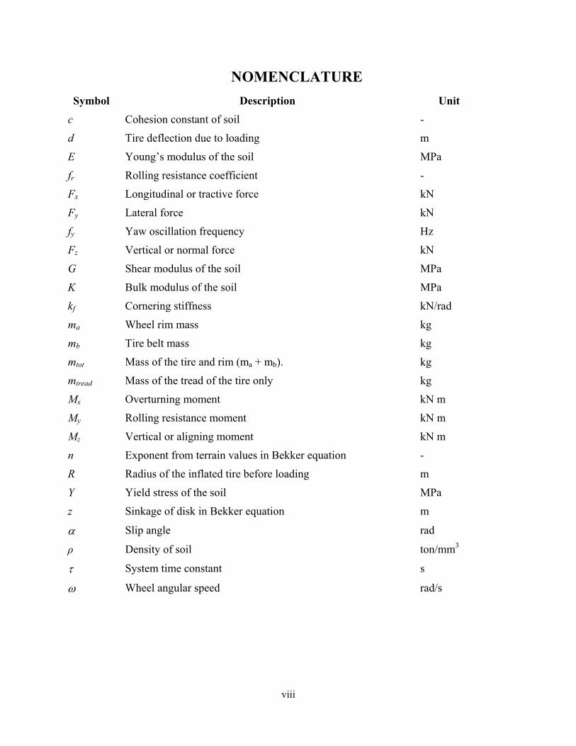
Symbol Description Unit
c Cohesion constant of soil -
d Tire deflection due to loading m
E Young’s modulus of the soil MPa
fr Rolling resistance coefficient -
Fx Longitudinal or tractive force kN
Fy Lateral force kN
fy Yaw oscillation frequency Hz
Fz Vertical or normal force kN
G Shear modulus of the soil MPa
K Bulk modulus of the soil MPa
kf Cornering stiffness kN/rad
ma Wheel rim mass kg
mb Tire belt mass kg
mtot Mass of the tire and rim (ma + mb). kg
mtread Mass of the tread of the tire only kg
Mx Overturning moment kN m
My Rolling resistance moment kN m
Mz Vertical or aligning moment kN m
n Exponent from terrain values in Bekker equation -
R Radius of the inflated tire before loading m
Y Yield stress of the soil MPa
z Sinkage of disk in Bekker equation m
Slip angle rad
ρ Density of soil ton/mm3
System time constant s
Wheel angular speed rad/s
ix
ACKNOWLEDGEMENTS
The author expresses his appreciation to Volvo Group Trucks Technology for their financial
support of this work and personal appreciation to David Philipps, Frederik Öijer, Inge
Johansson, and Stefan Edlund of Volvo Group Trucks Technology for their continued technical
support during the course of this research. Dr. Moustafa El-Gindy, my advisor, has been the
greatest source of knowledge and support in this work.
I would also like to give thanks to my family and friends for their encouragement and not only in
my studies, but also in my personal life. Special thanks to my two older sisters and my
grandmother, who sacrificed so much to allow me to be where I am today.

1
CHAPTER 1: INTRODUCTION
1.1 MOTIVATION
Tires in ground vehicles support the vehicle weight and cushion road surface irregularities to
provide a comfortable ride to driver and passengers. The tires also need to provide adequate
tractive, braking, and cornering forces, which are important for safe and stable operation of a
ground vehicle. A heavy truck tire experiences extreme loads for prolonged periods and is a key
component of the vehicle. Due to the large extent that modern society relies on transport, tire
dynamics and fuel efficiency make a large impact on traffic safety, environmental pollutants and
fuel expenses. Therefore, tire manufacturers conduct many physical laboratory tests such as in-
plane and out-of-plane stiffness and damping constant tests, cornering tests, and durability tests
in order to examine the tire performance.
Usually, the measurement tests in laboratory considerably consume time and cost. Experiment
equipment, their set-up, and data acquisition and analyses need highly experienced skills and
long testing time. Therefore, many researchers have tried to build alternative tire test
environments during the last few decades. Fortunately, modern computer technology enables a
new era of tire testing. Through tire model simulations, most of the laboratory tire tests can be
duplicated. Even tire tests that cannot be performed in laboratory, such as high speed and/or
loading operations, are possible with the computer simulations.
Whereas physical testing requires substantial post-processing and analysis, FEA models can be
configured to target just the right amount and type of data to be extracted, and post-processing
can be programmed easily through macros, algorithms or other interfaces which interact directly

2
with the FEA results. In addition, many of the errors during measurements, noise from external
sources, and incomplete or faulty test procedures can be eliminated from FEA models, or can be
corrected for with minimal effort or cost. Thus, the virtual modeling of tires and their interaction
with various terrains can be used to reduce costs, and increase the efficiency, of tire prototyping
and manufacturing. Furthermore, tire models can be implemented into complete vehicle models,
whether for crash testing or vehicle dynamics analysis.
The modeling of soils is fairly recent and the virtual modeling of the same more so.
Representation of soils in virtual environments, whether through traditional FEA modeling, or
more complex discrete element methods, is limited. With a more comprehensive soil model, the
applications would be numerous. For the purpose of this research, accurate soil models are
required to analyse the interaction of the pneumatic tire with soft soils. However, this is just one
example of the use of such soil models, as they could be used in civil engineering, adapted to
game engines for realistic deformation and handling in off-road racing, or even to virtually
analyse the effects of terraforming.
1.2 LITERATURE REVIEW
1.2.1 Pneumatic Tires
The pneumatic tire is a highly complex system of rubber, steel belts, nylon fibers, and many
other components which result in sandwich of materials which support a vehicle’s weight and
ensure traction in extreme maneuvers. As the only contact between the vehicle and the road
surface, tires are responsible for transmitting the vehicle forces such as acceleration, braking and
cornering forces to the ground. It also serves as the first component of the suspension system in
the vehicle, as the tire has some stiffness and damping which isolate the vehicle from shocks due

3
to irregularities in the road surface. Thus, the tire is responsible not only for the performance and
handling of the vehicle, but also the ride comfort and control.
When considering pneumatic tires, one must look at bias-ply and radial-ply tires. Bias-ply tires,
also called cross-ply tires, were widely used until the 1950’s. Following the introduction of the
radial-ply tire in 1946 by Michelin (Michelin AG, 2012) the trend shifted in its favour mainly
due to the numerous advantages that the radial-ply tire introduced. They have been shown to
provide improved handling, ride comfort, and conformity to the road while reducing internal
friction and thus rolling resistance (Wong J. , 2008). An example of the construction of a radial-
ply tire is shown in Figure 1.1, while Figure 1.2 shows a comparison between the bias-ply and
radial-ply tire and how the belts are arranged in each.
The basic construction of both types of tires consists of a carcass, inner beads, side walls, steel
belts and tread. The carcass is made from layers of textile plies. In bias-ply tires, nylon may still
be used, however radial-ply tires tend to use raylon or polyester. The beads are at the inner
diameter of the tire carcass and make contact with the wheel to provide a seal for the cushion of
air required for the inflation of the tire. The center of the bead is comprised of steel wire cord
which provides the strength required to keep the tire seated on the wheel rim. Side walls are the
outer portion of the carcass that is covered in a rubber compound and need to be very flexible,
yet durable enough to protect the carcass from damage such as cuts or scrapes. The flexibility of
the sidewall in a radial-ply tire provides a large portion of the stiffness and damping
characteristics of the tire. The steel belts of the tire provide the rigidity of the tread base, and are
located between the tread and the carcass. The tread itself is made from a rubber compound
designed to provide traction with the road surface, yet provide low wear (Heisler, 2002)

4
Figure 1.1 Construction of a typical radial-ply pneumatic tire. Retreived from
www.sturgeontire.com
Figure 1.2 Tire construction of bias ply (a) and radial ply (b) tires (Wong J. , 2008)
In a radial-ply tire there are radially oriented cords running directly from one bead to the other.
Layers of belts cross each other at a cord angle (± 20° as in Figure 1.2) and reinforce the tread.
Tönük and Ünlüsoy were amongst the first to create an FEA model (Tönük, 2001). They

5
successfully performed simulations over a range of slip angles (0° to 7° slip) and vertical loads
(1.5 kN to 4.5 kN) to determine lateral forces. The simulation data was compared with
experimental data, and it was found that the model successfully predicted lateral forces to an
acceptable degree of accuracy. Thus, it was found that FEA models had the potential to be a
valuable tool in the modeling and analysis of tires.
1.2.2 Measurement Standards
Two major industry standards are used for the measurement of rolling resistance of tires. The
SAE and ISO standards are used for experimental data collection, which is then further
processed to eliminate external influences and obtain comparable, uniform data.
The test equipment used for both of these experimental tests is a drum-spindle machine, which
consists of a large drum on which the tire rolls, and a spindle, to which the test tire is mounted.
The spindle lowers down until the tire makes contact with the drum, and the position of the
spindle may be locked in respect to the distance from the drum, to simulate a large load which
may cause deflection of the tire sidewall.
SAE document J1269 (SAE International, 2000) provides a standard method for gathering data
on a uniform basis so as to allow easy comparison and evaluation, and recommends one of three
methods to measure the rolling resistance. The force method measures the reaction force at the
tire spindle and converts it to rolling resistance, while the torque and power methods measure the
torque or power input, respectively, to the machine and converts it to rolling resistance. Similar
to SAE recommended practices for measuring rolling resistance, the ISO lists methods of

6
measuring rolling resistance in document ISO 28580:2009 (International Organization for
Standardization, 2009). Both methods use a similar approach to obtain data.
1.2.3 Rolling Resistance Prediction
Previous research into the rolling resistance of tires has been extensive; some prominent
literature on the subject is presented in Wong J. , 2008 and other publications such as (Dukkipati,
2008) and (Pacejka H. B., 2006). According to Wong, the rolling resistance of tires on hard
surfaces is primarily caused by the hysteresis in tire materials due to the deflection of the carcass
while rolling. In addition to internal hysteresis, friction between the tire and the road caused by
sliding, the resistance due to air circulating inside the tire, and the fan effect of the rotating tire
on the surrounding air are secondary sources of rolling resistance.
Wong presented models capable of estimating the rolling resistance coefficient of a truck tire at
speeds up to 100 km/h and tire pressure ranging between 90-120 psi as follows:
For a radial-ply truck tire: 0.006 0.23 10 (1.2.1)
For a bias-ply truck tire: 0.007 0.45 10 (1.2.2)
where fr is the rolling resistance force in Newtons, and V is the velocity of the vehicle in
kilometers per hour.
Rakah, 2001 also cites a truck rolling resistance model described in Fitch, 1994. It is presented as
a linear function based on the vehicle speed and mass, with consideration of road surface
material and condition:

7
9.8066 (1.2.3)
where M is the total mass, Cr is the rolling coefficient of the surface, and c2 and c3 are
coefficients for radial or bias-ply tires.
In a free-rolling tire, when there is no applied wheel torque, the rolling resistance is a
longitudinal force present between the tire and ground contact patch. Wong J. , 2008, as well as
Dukkipati, 2008 defined the ratio of the rolling resistance to the normal load on the tire as the
coefficient of rolling resistance:
(1.2.4)
where Cr represents the coefficient of rolling resistance, fx is rolling resistance force and fz is the
vertical (normal) force at the tire-ground contact patch.
1.2.4 Tire Modeling
Finite element analysis provides a means of virtual prototyping and testing of products and
systems. In the automotive industry, most major vehicle manufacturers utilize FEA simulation to
test components, and in certain cases almost entire vehicles under various conditions. For
example, virtual crash testing is now an essential step in the design and manufacturing process of
many automotive manufacturers. The vehicle components are often recreated from design plans
and assigned properties which accurately mimic the physical and material properties of the
component. They are then assembled into a complete model, once again replicating the joints,
welds and fasteners as accurately as possible. The complete model can be used to crash test the
vehicle using, for example, the National Highway Traffic Safety Administration standards, or

8
any other test conditions as desired. The results of the simulations are very accurate, and can be
repeated multiple times with no additional cost of producing another vehicle model, and minimal
cost to modify the test criterion or conditions. The simulations have a computational cost that is
quite high, however it is minimal in contrast to physical prototyping and testing.
The simulation of automotive tires and wheels in a virtual environment has a limited history. Due
to the relatively recent emergence and advancement in simulation programs and hardware, as
well as the complex construction of pneumatic tires, the development of FEA models of tires has
not been as widespread as modeling of other mechanical and automotive systems. Certainly, a
few accurate and realistic models have been developed, however they are modeled on a specific
tire, for a specific type of simulation, and thus their applications are highly limited.
Many analytical tire models were established to investigate the vertical vibration motion of a
vehicle such as a point contact tire model, an equivalent plane tire model, an effective road input
tire model, rigid and flexible roller contact models, and a finite element tire model. Among them,
point contact tire model has been widely adopted because of its simplicity (Captain, 1979), (Sui,
1999). The point contact tire model was established based on the assumption that a tire contacts
the road surface only through a single point, which is just located under the wheel center.
Because only the single point has contact with a road surface, the tire response is quite sensitive
to the road irregularities especially high frequency of road input that is usually filtered through a
contact patch in real tire applications. Therefore, the point contact tire model is useful mostly for
long wave road profile inputs. To overcome this limitation of the point contact tire model,
equivalent plane tire model and effective road input model were established. Equivalent plane
tire model was created with assumption that the tire can be simplified as a series of linear radial

9
springs that connect the wheel center and the imaginary equivalent plane. This equivalent plane
tire model can filter high frequency of road profile input and works more precisely for concave
road surface than convex road surface. However, the equivalent plane tire model still has
difficulty in determining the equivalent plane and out-of-plane behaviors since the model
consists of only two-dimensional in-plane radial springs (Davis, 1974).
In 1985, Loo developed an analytical tire model which consisted of a flexible ring under tension
with a nest of radially arranged linear springs and dampers to represent a pneumatic tire model.
He was concerned with the prediction of the tire’s vertical load displacement characteristics and
its rolling resistance. The ring, which represents the tread band of the tire, is assumed to be
massless and completely flexible. In 1997, Zegelaar constructed a rigid ring tire model to
represent a passenger car tire. In the rigid ring tire model, the tread and steel belts were modeled
as a rigid ring. Since the tread and steel belts parts were modeled as a rigid ring, a new parameter
such as a vertical residual stiffness was required to represent the large deformation of the tire in
the contact area. This rigid ring was placed on an elastic foundation that represented the tire
sidewall. The tire model was assembled with a 2.5 m-diameter test drum model and vertically
loaded to complete tire testing simulation environment. Then, the drum rotational speed
increased to reach tangential speed up to 150 km/h. They found from the simulation that the
vertical force on the tire and effective rolling radius of the tire increased as the tire rotational
speed increased. This simulation results correlated quite well with their measurement. Brake
torque variations were applied to excite the in-plane tire behavior. Then, the measured frequency
response functions were used to determine the required parameters for the rigid ring tire model.

10
Figure 1.3 Rigid ring tire model showing the in-plane parameters (Zegelaar, 1997)
Schmeitz, 2004 presented a quarter vehicle model by combining the rigid ring tire model,
suspension, sprung mass and elliptical cams together. The elliptical cams were adopted to
generate an effective road profile. They predicted vertical tire motions and longitudinal forces for
different heights of step road inputs. Then, the predicted results were compared with
measurements and showed good correlations. They also conducted modal analyses on the quarter
vehicle system to find the first vertical mode at 71.5 Hz and horizontal mode at 84.4 Hz.
Many researchers have undertaken examination of the full FEA models since late 1970’s because
traditional structural analysis techniques could no longer offer sufficiently detailed results for
modern advanced tire design. These FEA models can reflect real-world operating conditions of
tires most accurately even though FEA models require longer computational time. Still, tire
design is highly dependent upon empirical procedures. However, the FEA model approach can
predict a tire behavior and characteristic parameters precisely and cost-effectively.
11
Nakajima, in 1986, developed the tire transient sliding contact model on an arbitrarily shaped
surface. Thus, tire sliding events involving impact with holes and bumps were simulated using
the finite element simulation software, ADINA. The tread and sidewalls were modeled by a
linear viscoelastic ring on an elastic foundation. They discussed the vertical and horizontal force
history of the tire spindle with the tire sliding over a bump and a hole at different velocities. The
computed and experimental results were in good agreement.
In 1997, Kao simulated a simple tire test by using FEA software and demonstrated that it is
possible to predict tire transient dynamic responses from the tire design data. Here, for the first
time, an FEA tire model incorporated geometry, material properties of the various components,
fiber reinforcement, layout, and other features of a commercial passenger car radial-ply tire of
size P205/65R15. Before Kao and Muthukrishnan, almost all the research about FEA tire models
were built using only a single type of element under reasonable simplifications and assumptions;
these simplifications meant the loss of some detail complexity at the same time. Kamoulakos and
Kao again verified the same setup with another finite element software, PAM-SHOCK. They
improved the model's correlation to reality. They also extended this simulation further for six
more impacts, corresponding to 21 tire revolutions, to demonstrate the reliability of the program
in providing an instability-free scenario for the tire impact problem.
The problem of predicting the transient response of a tire impact with a rigid surface is a rather
complicated step. Such response is largely and directly related to vehicle handling (steering),
control, and ride comfort. The interactions within the tire structure, for example, the friction
between carcass and belt, the elasticity and plasticity interactions, can make this problem even
more difficult to handle. In 2002, (Chang, 2002) developed tire-drum model to predict tire
12
standing waves and tire free vibration modes. Visualized simulations of the standing waves
phenomenon were carried out for the first time. The detection of the tire in-plane free vibration
modes was achieved by recording the reaction force histories of the tire axle at longitudinal and
vertical directions when the tire rolling over a cleat on the road, and then the FFT algorithm was
applied to examine the transient response in frequency domain. They reported 80 Hz resonance
vertically and 40 Hz resonance longitudinally with a P185/70R14 tire. The results were
compared to more than ten previous studies by either theoretical or experimental approach or
showed good agreement. In 2001, Chae et. al published their studies of an SAE Formula 1 racing
car tire standing waves and wavelength predictions. The tire model was constructed from special
three-layer membrane elements without thick solid tread parts, as it is the case of the SAE
Formula 1 tires. The results showed that as inflation pressure increases or load decreases, the
standing wave initiation speed increases. In 2002, Zhang developed a nonlinear FEA model of a
radial truck tire to analyze the tensile stress distribution, deformation fields and inter-ply shear
stresses, and the tire-road contact pressure distribution on the contact area as a function of the
static vertical load. In this model, the hyper-elastic solid rubber elements were adopted to
represent large magnitude of nonlinear deformations. In 2004, Chae et. al developed a detailed
nonlinear FEA model of a radial-ply truck tire by using an explicit FEA simulation software,
PAM-SHOCK. The tire model was constructed to its extreme complexity with solid, layered
membrane, and beam elements. In addition to the tire model itself, a rim model was included and
rotated with the tire with proper mass and rotational inertial effects. The predicted tire
characteristics and responses, such as vertical stiffness, cornering force, and aligning moment,
correlated very well to physical measurements. In this study, the in-plane sidewall translational
stiffness and damping constants of the FEA tire model were determined by rotating the tire on a

13
cleat-drum. The other in-plane parameters, such as tire rotational stiffness and damping constant,
were determined by applying and releasing a tangential force on the rigid tread band of the FEA
tire model.
1.2.5 Soil Modeling
In order to understand the behaviour of soils, models are often used. A key part of any model is
the measurement and characterization of the terrain properties; thus a few of them are discussed
in this section.
Current methods for measuring the properties of soils include the cone penetrometer, the
bevameter, and the traditional civil engineering techniques. For vehicle mobility evaluations, the
penetrometer and the bevameter are the most commonly used (Wong J. Y., 2010). The cone
penetrometer technique was developed for military evaluation of terrain in the Second World
War and uses a 30-degree cone at the bottom end with a base area of 3.23cm2 and is pushed into
the terrain to be evaluated. The resistance of the terrain to penetration is supposed to represent
the combined shear and compressive properties of the soil, however the contribution of each
factor to the “cone index” cannot be determined, and it has been proven to be inadequate for
certain terrains such as sand. This inadequacy lead to the further characterization of individual
factors based on laboratory testing of later techniques.
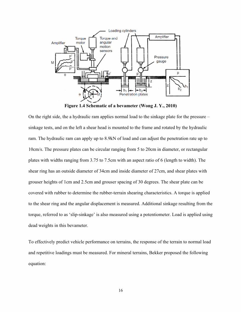
The bevameter technique developed by Bekker in the 1950’s and 60’s uses two separate field
tests to represent the normal and shear stresses exerted on terrain when a vehicle passes over it
(Bekker, 1960). The plate penetration test, also known as the pressure-sinkage test, a plate
representing the contact area of the tire is used to test the compressive properties of the terrain. In
14
the shear test, the stress-shear displacement relationship and shear strength of the terrain are
measured.
The traditional civil engineering approach uses laboratory testing to find the properties of soils,
and evaluates such parameters as shear strength, shear modulus, density, void ratio, etc. The
shear strength is usually measured using a triaxial apparatus or a direct shear box. However, in
addition to being costly, the testing of terrain in a laboratory presents the possibility of disturbing
the terrain from its natural state. Thus, civil engineering approaches are not commonly used to
evaluate vehicle mobility.
The cone penetrometer technique was originally used to test terrain mobility and trafficability on
a ‘go/no-go’ basis and was a handheld device which consisted of a 5/8in diameter rod with the
aforementioned cone on one end. On the other end a proving ring and dial indicated the force
required to push the cone into the terrain. A recommended rate of penetration of approximately
6ft/min would allow a reading of the force per unit cone base area, the cone index (CI), which is
used as an undimensional parameter but is actually the force in pounds exerted on the
penetrometer divided by the area of the cone base in square inches. Multiple readings are taken,
starting with when the base of the cone is flush with the terrain surface, then every 3in until 12in,
then every 6in until a depth of 30in (or to the capacity of the cone penetrometer). Further testing
of the terrain can be done to simulate repeated traffic and the change in strength of the terrain,
known as the remoulding index (RI), where the cone technique is applied with multiple loadings,
and can employ a different sized cone in certain cases.
The product of the cone index and remoulding index, known as the rating cone index (RCI)
represents the strength of the terrain under repeated vehicular traffic. The vehicle cone index
15
(VCI) indicates the terrain trafficability and is the minimum index of a soil in the critical layer
that permits a given vehicle to make a specific number of passes without immobilization, where
the depth of critical layer varies with vehicle type and weight.
The cone peneterometer alone is not sufficient to characterize a terrain, as mentioned previously,
and further studies show that the cone index is actually a compound parameter reflecting the
shear, compressive, and tensile strengths of the terrain and soil-metal friction and adhesion. The
cone index is also insensitive to shear or compressive strength as soil moisture content increases
and surface irregularity around the compaction zones change the relationship between the
penetration resistance and soil properties. Furthermore, it is not possible to accurately derive the
values of terrain parameters from the cone index, and thus is not an ideal method for
characterizing terrain.
The bevameter technique uses two separate tests to measure the shear and compressive strength
of the terrain. In the pressure-sinkage test the properties of the terrain are measured using a plate
representing the tire contact patch, and is used to predict the normal pressure distribution on the
vehicle-terrain interface. In the shear tests, the shear stress-displacement relationship at various
normal pressures is measured, and provides the inputs required for predicting the shear stress
distribution on the vehicle-terrain interface. Both tests may be repeated to measure and predict
multipass performance and the additional vehicle sinkage due to slip.
A specific bevameter originally built at the University of Newcastle and extensively modified at
Carleton university is shown in Figure 1.4.
16
Figure 1.4 Schematic of a bevameter (Wong J. Y., 2010)
On the right side, the a hydraulic ram applies normal load to the sinkage plate for the pressure –
sinkage tests, and on the left a shear head is mounted to the frame and rotated by the hydraulic
ram. The hydraulic ram can apply up to 8.9kN of load and can adjust the penetration rate up to
10cm/s. The pressure plates can be circular ranging from 5 to 20cm in diameter, or rectangular
plates with widths ranging from 3.75 to 7.5cm with an aspect ratio of 6 (length to width). The
shear ring has an outside diameter of 34cm and inside diameter of 27cm, and shear plates with
grouser heights of 1cm and 2.5cm and grouser spacing of 30 degrees. The shear plate can be
covered with rubber to determine the rubber-terrain shearing characteristics. A torque is applied
to the shear ring and the angular displacement is measured. Additional sinkage resulting from the
torque, referred to as ‘slip-sinkage’ is also measured using a potentiometer. Load is applied using
dead weights in this bevameter.
To effectively predict vehicle performance on terrains, the response of the terrain to normal load
and repetitive loadings must be measured. For mineral terrains, Bekker proposed the following
equation:
17
Ф z (1.2.5)
where p is pressure; b is the radius of a circular plate or the smaller dimension of a rectangular
plate; n, kc and kφ are pressure–sinkage parameters for the Bekker equation; keq = kc/b + kφ, and z
is sinkage. It has been shown by Bekker that the pressure-sinkage parameters are insensitive to
the width of the rectangular plates with large aspect ratios (between 5 and 7), and that using
circular plates with radii equal to the widths of the rectangular plates shows little difference in
measurements. Note that kc and kφ have variable dimensions depending on the value of the
exponent n.
In 1965 Reece proposed the following equation for the pressure-sinkage relationship, which is
based on experimental evidence:
(1.2.6)
where n, kc’ and kφ’ are the pressure–sinkage parameters for the Reece equation; ɣs is the weight
density of the terrain; and c is the cohesion of the terrain. For frictionless clay, kφ’ should be
negligible and the relationship between p and (z/b) is not affected by plate width b. For dry,
cohesionless sand, kc’ should be negligible and the pressure p increases linearly with the increase
in width of the plate. Note that the parameters kc’ and kφ’ are dimensionless, unlike parameters kc
and kφ from Bekker’s equation. Also note that Reece’s equation applies only to homogeneous
(unlayered) terrain.
For both Bekker’s and Reece’s equations, it is essential that the proper values of the terrain
parameters are obtained from the experimental data. Traditionally, the experimental data are
18
plotted on a log-log scale and a straight line is fitted by eye, thus there may be a large variance
based on the personnel manipulating the data. Computerized procedures using weighted least-
squares methods can be incorporated to provide more rational, consistent parameter values.
Table 1 provides some mean values of parameters characterizing the pressure-sinkage relations
of some mineral terrains.
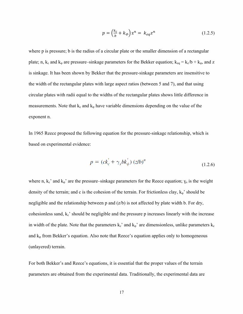
Table 1 Mean values of parameters characterizing pressure-sinkage relations of various terrains (Wong J. Y., 2010)
Janosi et. al were among the first to develop predictive formulations for the shearing of soils
(Janosi, 1961). The shear forces exhibited by the soil were observed at various normal loads and
19
models were developed which allowed for approximated predictions with some accuracy and
consistency. Bekker’s developed model primarily intended to predict the interaction of forces
normal to the soil, while Janosi and Hanamoto’s predicted shearing properties of the soil. In
1964, Osman verified the cohesion and angle of shearing resistance parameters obtained from
available testing methods, including the translational shear box (direct shear method), the triaxial
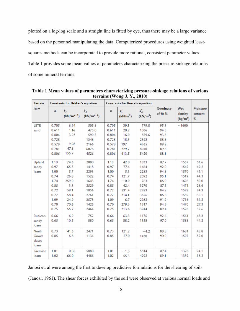
test, the N.I.A.E shear box, the bevameter, the shear vane, and others. In this research, the direct
shear method using a translational box is of particular interest. The box consists of two halves,
one of which is fixed and the other free to slide relative to the other. The box is filled with soil,
and a load is applied to the top half. Once the soil is settled, a constant strain is applied while the
transmitted shear force is measured. An example setup of this laboratory test is shown in Figure
1.5.
Figure 1.5 Setup for a Translational Shear Box test. Retrieved from
http://theconstructor.org/geotechnical/shear-strength-of-soil-by-direct-shear-test/3112/
The modeling of soft soils in virtual environments has been restricted. Most soil models have
been developed using traditional FEA modeling, which comes with a number of limitations due
to the nature of the underlying technique. For example, FEA soils are not able to accurately
represent the shear properties of soils, and are unable to provide penetration when loaded; rather
FEA soils act in a manner similar to a sponge, where the whole block of soil acts as a single unit
20
and each neighbouring element is directly connected to and influenced by the adjacent element.
Soft soils are best represented as particulate matter consisting of a large number of non-
homogeneous free particles which are able to move without respect to any other particle, and
able to interact with neighbouring particles based on the material properties of each. Thus, while
sufficient in certain circumstances, using FEA soil models would not be ideal for the analysis of
tire-soil interactions.
1.2.6 Smoothed Particle Hydrodynamics
Smoothed Particle Hydrodynamics (SPH) is a relatively recent, meshless modeling method for
virtual environments. One of the first mentions of this technique is by Schlatter (1999), in which
the origins are traced to the study of galaxy formation. Recent uses for this method include fluid
dynamics, hypervelocity impacts, and other complex, particulate-related problems such as soil
flow analysis.
Traditional meshing techniques (finite element analysis) works by dividing the simulation object
or region into smaller portions using a grid or specialized algorithm. Elements are able to interact
with adjacent elements, but they are attached to each other and have no interaction beyond
directly neighbouring elements. This creates a scenario in which there is a “sponge” effect,
shown in Figure 1.6, causing the block as a whole to deform. Furthermore, the block cannot be
penetrated or substantially sheared.
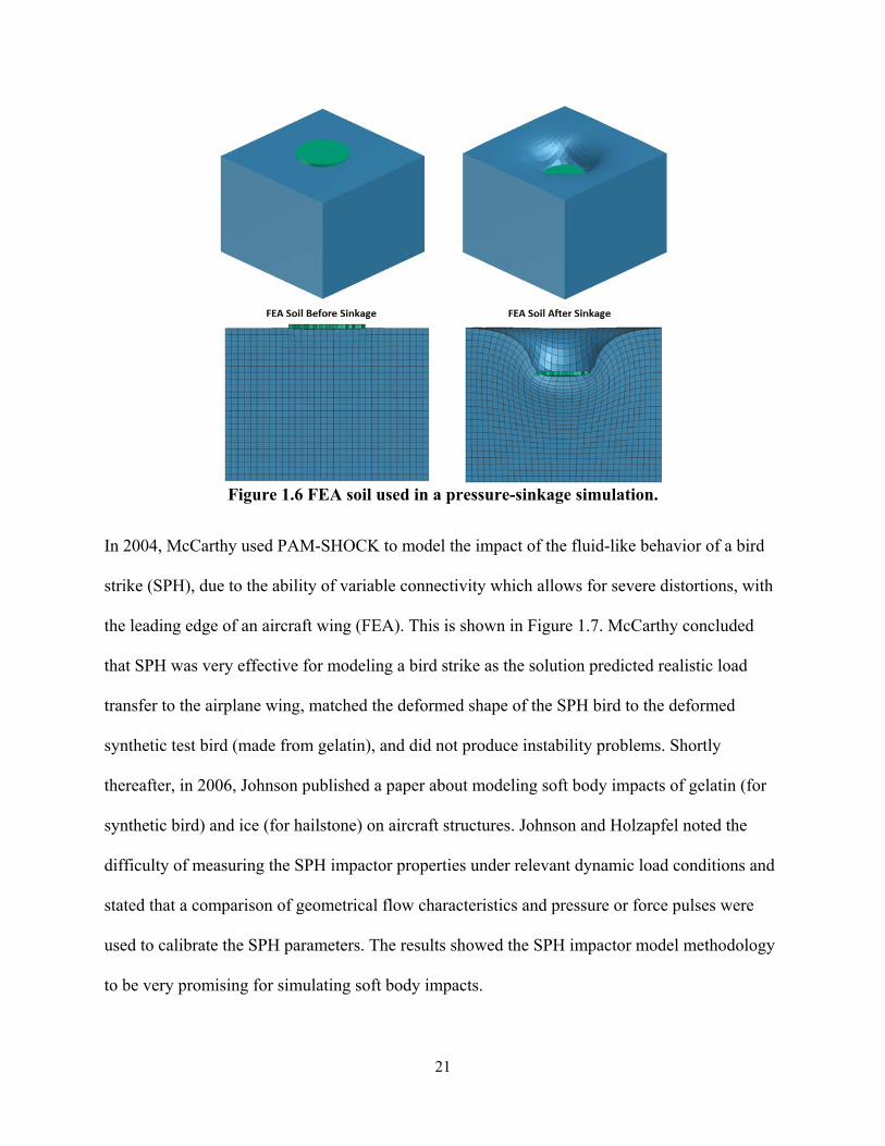
21
Figure 1.6 FEA soil used in a pressure-sinkage simulation.
In 2004, McCarthy used PAM-SHOCK to model the impact of the fluid-like behavior of a bird
strike (SPH), due to the ability of variable connectivity which allows for severe distortions, with
the leading edge of an aircraft wing (FEA). This is shown in Figure 1.7. McCarthy concluded
that SPH was very effective for modeling a bird strike as the solution predicted realistic load
transfer to the airplane wing, matched the deformed shape of the SPH bird to the deformed
synthetic test bird (made from gelatin), and did not produce instability problems. Shortly
thereafter, in 2006, Johnson published a paper about modeling soft body impacts of gelatin (for
synthetic bird) and ice (for hailstone) on aircraft structures. Johnson and Holzapfel noted the
difficulty of measuring the SPH impactor properties under relevant dynamic load conditions and
stated that a comparison of geometrical flow characteristics and pressure or force pulses were
used to calibrate the SPH parameters. The results showed the SPH impactor model methodology
to be very promising for simulating soft body impacts.

22
Figure 1.7 Impact of a gelatin bird on an aircraft wing (left) and SPH of the same (right).
(McCarthy, 2004)
(Bui H. H., 2007) and (Bui H. H., 2008) studied the use of SPH for modeling the interaction of
soil and water. Bui found that when SPH is applied to solids, the SPH particles mimic the
behaviour of atoms. That is, atoms repel each other when compressed, and attract each other
when stretched. While some instability was initially present, after correction the results of Bui’s
simulations showed good agreement with experimental results.
The SPH representation found in ESI Group’s PAM software uses a kernel (W4 B-Spline by
default) which defines the interaction between SPH elements and other elements in the model.
1.3 OBJECTIVES AND SCOPE
The objective of this thesis is to develop tire and soil models for use in tire-terrain interaction
analysis. Currently, very limited models exist for this type of analysis. Developed tire models
will be validated using static load-deflection and cleat envelopment criteria, as well as dynamic
vibrational analysis. Soil models will be created using the Smoothed Particle Hydrodynamics
method, compared with FEA models, and validated on the pressure-sinkage and shear strength

23
criterion. Actual tires and soils will be modeled as closely as possible in the interest of accuracy,
while maximizing efficiency of the available computing resources.
1.4 OUTLINE
Chapter 2 provides an introduction to the approach used to model and validate tires. Chapter 3
describes the methods used to model and validate soils. Chapter 4 discusses the various tests on
rigid surfaces using the 3-groove on-road tire, while chapter 5 describes the use of the Regional
Haul Drive off-road tire in conjunction with soil models for tire-soil interaction analysis. Chapter
6 discusses the results, conclusions, and recommendations for future work.
24
CHAPTER 2: TIRE MODELING
The software used to model the tire is the PAM-SYSTEM, comprising of industry-leading code
for finite element analysis developed by ESI Group. The software is used for virtual crash testing
by many commercial vehicle manufacturers and recognized for its accuracy and flexibility in
modeling of complex systems. For this research, the MESH, CRASH, SHOCK and VIEWER
applications were primarily used to create, set up and analyze the tire model.
2.1 TIRE CONSTRUCTION
The FEA tire model created is derived from a radial-ply aircraft tire model developed by ESI
North America, and later modified for passenger vehicles by (Chang, 2002), then to heavy trucks
by (Chae S. , 2006). The tire was subjected to vibration and transmissibility simulation testing
with the use of a cleat-drum model, as well as demonstration of the standing wave phenomenon
at high speeds using a tire on a smooth drum model. For this paper, the initial 3-groove truck tire
is modified to improve stability and a full three-dimensional radial-ply truck tire is modeled with
the non-linear FEA software PAM-SHOCK so that it matches a Goodyear G357, 295/75R22.5G
tire.
The tire has a number of layers which serve their own purpose in determining the handling
characteristics of the tire. The carcass of the tire, consisting of the inner liner and the plies
running from one bead to the other, must be very flexible yet able to sustain high loads while
resisting fatigue. Flexible, high-modulus cords are embedded in a low-modulus matrix to form
the carcass of the tire. The number of plies varies based on the tire type and expected operating
conditions, such as inflation pressure and loading. The plies can be arranged at a bias angle or
25
radial angle; in this research, radial-ply tires are modeled due to their extensive use in recent
years.
Due to the radial orientation of the carcass’ plies, the tire model exhibits good ride quality, but
handling characteristics of the tire are poor. The belts of the tire are composite materials made up
of reinforcing steel cords and rubber matrix, located between the carcass and the tread base. In a
radial-ply tire, the belt plies are oriented with a low crown angle to improve cornering
performance, and are essential to the proper functioning of the tire; without belt plies, the tire
would deform excessively and make for an unstable ride. The tread of the tire is the only part of
the tire to make contact with the road surface. The treadbase is located between the tread and the
belt plies, and is made of a softer rubber than the tread. The tread base provides the bonding
between the tread and belt plies, as well as some cushioning.
The beads of the tire hold the tire to the wheel rim. They provide an anchor point for the carcass
plies and keep the tire and wheel from separating in an undesired manner. Such a failure could
result in the loss of air pressure, tire blow-out, or failure to deliver power to the road surface due
to bead slippage. The performance requirements for the tire beads are uniformity, mountability,
rim roll-off resistance, tire-to-rim fitment, maximum strength at lowest weight, lateral and
circumferential stiffness, torsional and in-plane rigidity, fatigue resistance, and high adhesion
level as stated in Ford, 1988.
The bead bundles consist of either flat or round hard drawn steel wires put together to provide
the desired strength and rigidity. The bead and cords are encompassed in a rubber compound
which starts very thick near the bead (apex) and thins out until it reaches minimal thickness at

26
the sidewall. In fact, the carcass wraps around the beads and ends in the middle of the sidewalls.
Thus, the Young’s modulus in this area is about double that of other areas.
At the base of the tire model’s bead, a beam element is used to represent the bead bundle in an
actual tire. This element was chosen due to the behavior properties of the beam, which allows for
accurate simulation of the bead structure. The FEA tire construction is based on a simple set of
interconnected membranes with varying properties, and solid elements to represent the tread,
tread base, and apex.
The membranes are toroidal sheets of varying virtual thickness which are connected to adjacent
membrane sheets by edge-to-edge connections. Additionally, the lower-most membrane is
connected to the bead material, which is then attached to the wheel rim. One of the 60 radial
sections which comprise the tire models is shown in Figure 2.1.
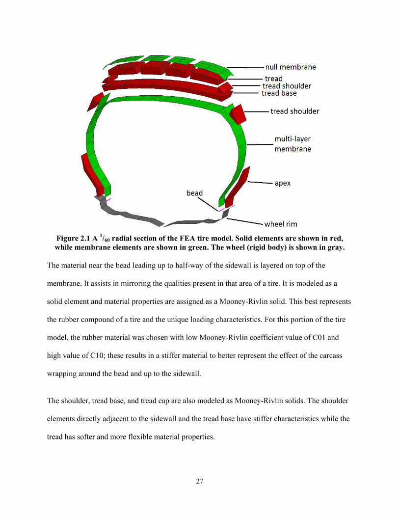
27
Figure 2.1 A 1/60 radial section of the FEA tire model. Solid elements are shown in red, while membrane elements are shown in green. The wheel (rigid body) is shown in gray.
The material near the bead leading up to half-way of the sidewall is layered on top of the
membrane. It assists in mirroring the qualities present in that area of a tire. It is modeled as a
solid element and material properties are assigned as a Mooney-Rivlin solid. This best represents
the rubber compound of a tire and the unique loading characteristics. For this portion of the tire
model, the rubber material was chosen with low Mooney-Rivlin coefficient value of C01 and
high value of C10; these results in a stiffer material to better represent the effect of the carcass
wrapping around the bead and up to the sidewall.
The shoulder, tread base, and tread cap are also modeled as Mooney-Rivlin solids. The shoulder
elements directly adjacent to the sidewall and the tread base have stiffer characteristics while the
tread has softer and more flexible material properties.
28
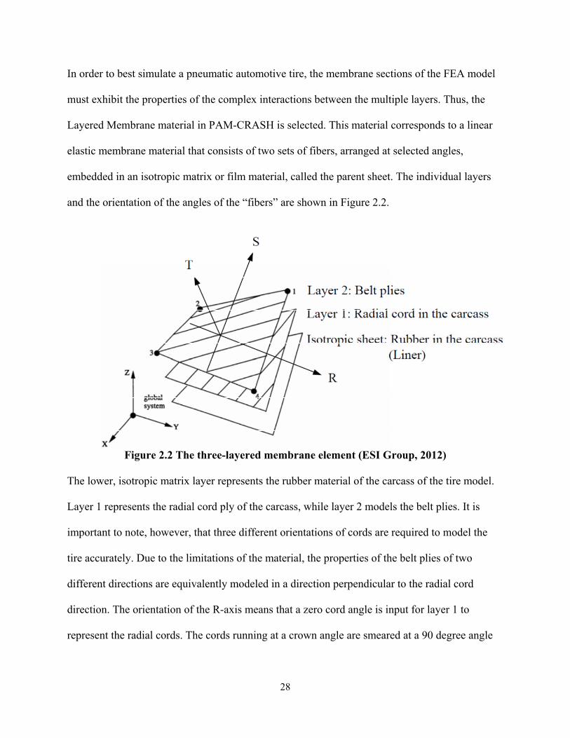
In order to best simulate a pneumatic automotive tire, the membrane sections of the FEA model
must exhibit the properties of the complex interactions between the multiple layers. Thus, the
Layered Membrane material in PAM-CRASH is selected. This material corresponds to a linear
elastic membrane material that consists of two sets of fibers, arranged at selected angles,
embedded in an isotropic matrix or film material, called the parent sheet. The individual layers
and the orientation of the angles of the “fibers” are shown in Figure 2.2.
Figure 2.2 The three-layered membrane element (ESI Group, 2012)
The lower, isotropic matrix layer represents the rubber material of the carcass of the tire model.
Layer 1 represents the radial cord ply of the carcass, while layer 2 models the belt plies. It is
important to note, however, that three different orientations of cords are required to model the
tire accurately. Due to the limitations of the material, the properties of the belt plies of two
different directions are equivalently modeled in a direction perpendicular to the radial cord
direction. The orientation of the R-axis means that a zero cord angle is input for layer 1 to
represent the radial cords. The cords running at a crown angle are smeared at a 90 degree angle
29
from the R-axis for layer 2, however because they are only required for the area under the tread
base, the material properties of layer 2 are largely negligible for the sidewalls.
Furthermore, the membrane elements at the tread shoulders and near the bead have a
considerably higher Young’s Modulus than those of the other membrane sections, to mimic the
behavior seen in those areas. The thickness of each membrane is varied virtually through the
element card, and as with an actual tire, it is thinnest at the sidewall. It is important to note that
the hysteresis of rubber is considered only for the membrane elements, and is not simulated in
the solid elements.
Once all parts consisting of the beam elements for the bead, membrane elements for the plies and
cords, and solid rubber elements are assembled to create a complete section of the tire model, it
is revolved around the model origin for a total of 60 individual sections. This completes a tire
model, and once all necessary connections between adjacent sections are defined, the tire is
ready for assembly with the wheel model. Dimensions of the model are shown in Figure 2.3.
30
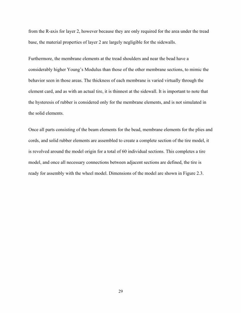
Figure 2.3 Dimensions of the UOIT 3-groove Truck Tire.
The FEA rim model used for this report is based on a standard set of size and contour dimensions
obtained from The Tire and Rim Association. The 8.25 x 22.5in rim is shown below in Figure
2.4. The rim is a simple solid part with rigid body properties. The material properties were
chosen as steel, which results in a rim weight of 32kg.
Figure 2.4 FEA Truck Tire Rim Model

31
It is important to make sure that contacts between the rim and tire are defined correctly so that
the tire can inflate and maintain pressure while subject to loading and normal vehicle operations.
While actual interaction between the rim and bead is complex, in the FEA model the tire-rim
interaction is modeled as a solid connection between the rim and the bead for simplicity.
The test surfaces or “road profiles” used for the tests are simple sheets made by plotting nodes
and creating a coarse mesh. The properties of road elements are assigned as rigid body to
eliminate road profile deformation under various tire loading conditions. For this portion of the
research, it is assumed that the road surface is hard, rigid and non-deformable. The load-
deflection simulations are performed on a perfectly smooth, flat road. The rolling resistance
simulations are performed on different road models, varying from perfectly smooth to emulating
the road profile of a randomly-noisy road. For all road surfaces developed, the road friction
coefficient, µ, was chosen to be 0.6, to represent the micro-level roughness of a typical road
surface.
During the validation and simulations, the tire model is inflated to the desired pressure within the
first few milliseconds of simulation by using a pressure face which acts on the inside face of the
tire carcass and rim.
2.2 VALIDATION AND SIMULATION
2.2.1 First Mode of Frequency
The first criteria used to validate the FEA tire model and see the results of the tire on an uneven
surface is the first mode of frequency, a test which demonstrates the dynamic response of the tire

32
model. It is also referred to as the Power Spectral Density and represents the different possible
responses of the tire may experience when excited with a particular input.
In order to obtain the modes of frequency, the tire must experience vibration input; thus, an FEA
model of the cleated-surface drum test rig shown in Figure 2.5 was created. The drum diameter is
2.5m, while the semi-circular cleat on the drum has a height of 10mm. An angular velocity is
applied to the center of the drum so that the tire model rolls freely at 50 km/h. The model’s
spindle is fixed so that the vertical reaction force at tire center due to the cleat excitation can be
simulated. Using the Fast Fourier Transform algorithm on the reaction force at the spindle, the
vertical free vibration mode can be determined.
Figure 2.5 Cleated-Surface Drum Simulation
With a tire inflation pressure of 0.759 MPa (110 psi), an equivalent spindle load of 26.7 kN, and
by applying the FFT algorithm to the results, the plot shown in Figure 2.6 is generated.

33
Figure 2.6 FFT Results of Vertical Reaction Force at Tire Spindle
As seen in the above graph, the free vibration mode is detected at about 73 Hz, which falls within
a reasonable range as discovered in previous studies (Kao, 1997) , (Cremers, 2005).
2.2.2 Static Deflection and Enveloping Force
The generated FEA tire was verified to accurately represent a general, radial-ply pneumatic truck
tire through a number of deflection tests. The FEA tire, wheel and the rigid road are combined to
form the model shown in Figure 2.7(a) below. The tire model is constrained to allow movement
in the Z-direction only, and a vertical load is applied at the center of the tire. The deflection of
the tire center is measured once the model has stabilized and the results are compared with
experimental results to determine the accuracy of the FEA model with respect to vertical
stiffness. In addition to a flat surface, the deflection tests were performed on rectangular and
triangular cleats, as shown in Figure 2.7(b), to demonstrate the enveloping characteristics of the
tire model.

34
(a) (b)
Figure 2.7 (a) The complete FEA tire, wheel and rigid road assembly as used for the static deflection simulations. (b) The rectangular and triangular cleat profiles
The simulations conducted with regards to static deflection of a loaded tire are similar to those
outlined by SAE standards (SAE International, 2005) and can be verified by observing previous
data collected regarding the subject. Figure 2.8 below is one such example which shows the
load-deflection curve of a radial and bias-ply truck tire on a flat surface. Furthermore,
experimental data collected by Alkan and Kang show that at a certain point after the cleat is fully
enveloped, the tire behaves as if it were on a flat surface (Alkan, 2011), (Kang, 2009).
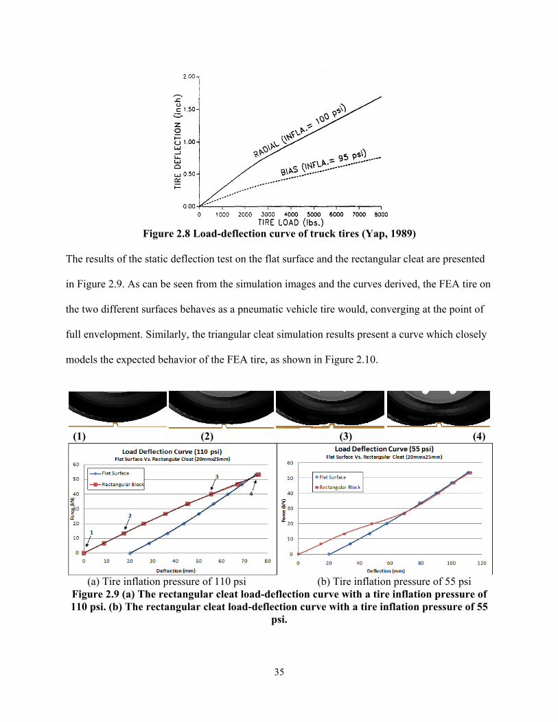
35
Figure 2.8 Load-deflection curve of truck tires (Yap, 1989)
The results of the static deflection test on the flat surface and the rectangular cleat are presented
in Figure 2.9. As can be seen from the simulation images and the curves derived, the FEA tire on
the two different surfaces behaves as a pneumatic vehicle tire would, converging at the point of
full envelopment. Similarly, the triangular cleat simulation results present a curve which closely
models the expected behavior of the FEA tire, as shown in Figure 2.10.
(1) (2) (3) (4)
(a) Tire inflation pressure of 110 psi (b) Tire inflation pressure of 55 psi
Figure 2.9 (a) The rectangular cleat load-deflection curve with a tire inflation pressure of 110 psi. (b) The rectangular cleat load-deflection curve with a tire inflation pressure of 55
psi.

36
(a) Tire inflation pressure of 110 psi (b) Tire inflation pressure of 55 psi
Figure 2.10 (a) The triangular cleat load-deflection curve with a tire inflation pressure of 110 psi. (b) The triangular cleat load-deflection curve with a tire inflation pressure of 55
psi.
It is of note that the flat surface deflection curves are shifted by 20mm and 25mm for the
rectangular and triangular cleats, respectively, to account for the higher initial displacement of
the tire on the cleat tests.
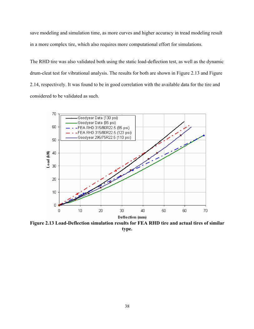
2.3 REGIONAL HAUL DRIVE (RHD) TIRE
For the simulations on soft soil, a Regional Haul Drive (RHD) tire is used. The original tire was
developed by Chae in 2005, then improved by Slade in 2009. It is based on a 4-groove off-road
tire and has been modified to represent a Goodyear RHD 315/80R22.5 tire, which is shown in
Figure 2.11. The dimensions of this tire are shown in Figure 2.12.
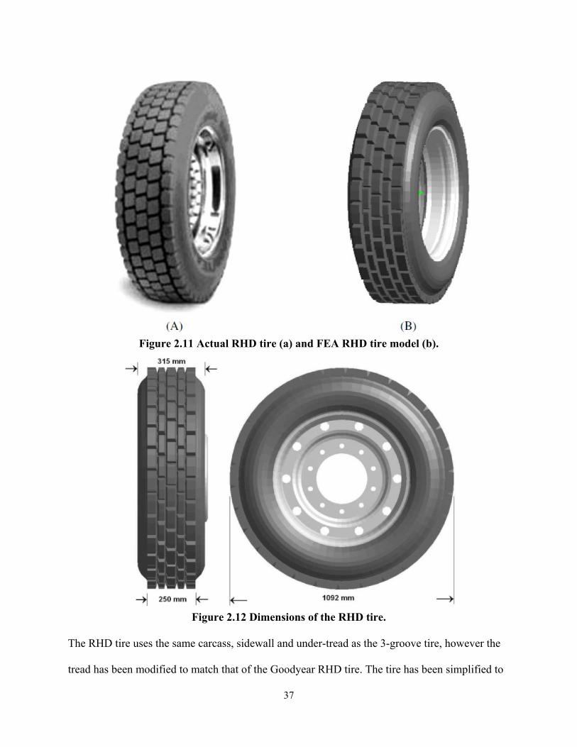
37
Figure 2.11 Actual RHD tire (a) and FEA RHD tire model (b).
Figure 2.12 Dimensions of the RHD tire.
The RHD tire uses the same carcass, sidewall and under-tread as the 3-groove tire, however the
tread has been modified to match that of the Goodyear RHD tire. The tire has been simplified to
38
save modeling and simulation time, as more curves and higher accuracy in tread modeling result
in a more complex tire, which also requires more computational effort for simulations.
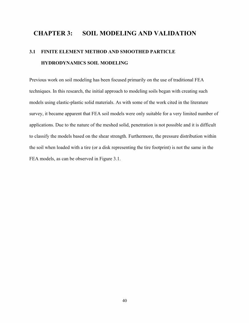
The RHD tire was also validated both using the static load-deflection test, as well as the dynamic
drum-cleat test for vibrational analysis. The results for both are shown in Figure 2.13 and Figure
2.14, respectively. It was found to be in good correlation with the available data for the tire and
considered to be validated as such.
Figure 2.13 Load-Deflection simulation results for FEA RHD tire and actual tires of similar
type.

39
Figure 2.14 Vertical free vibration frequency response analysis for the RHD tire model at a
load of 19 kN and inflation pressure of 85 psi.
40
CHAPTER 3: SOIL MODELING AND VALIDATION
3.1 FINITE ELEMENT METHOD AND SMOOTHED PARTICLE
HYDRODYNAMICS SOIL MODELING
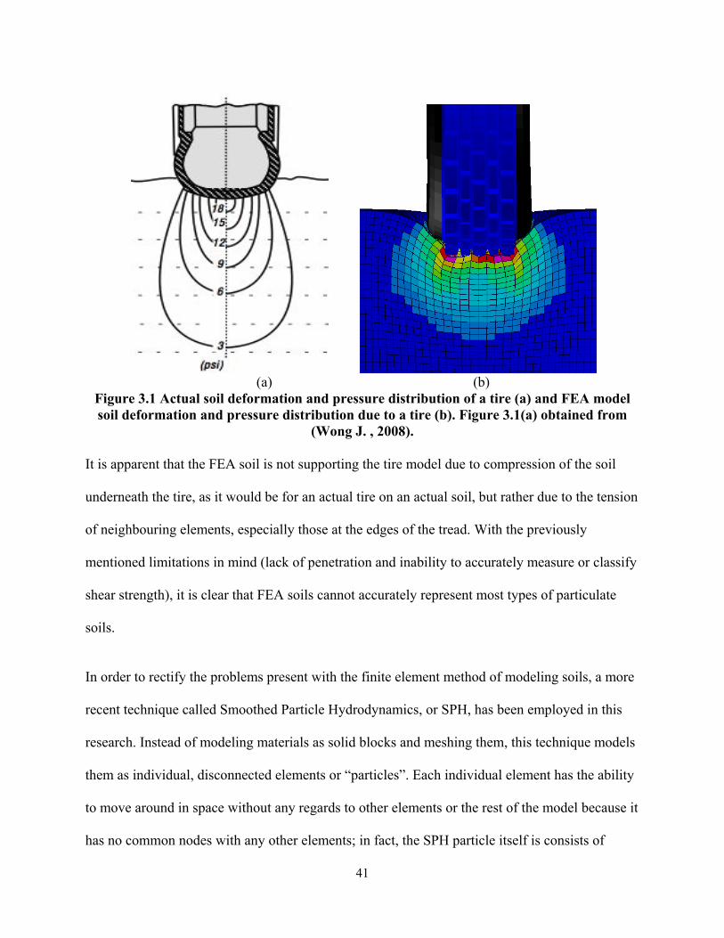
Previous work on soil modeling has been focused primarily on the use of traditional FEA
techniques. In this research, the initial approach to modeling soils began with creating such
models using elastic-plastic solid materials. As with some of the work cited in the literature
survey, it became apparent that FEA soil models were only suitable for a very limited number of
applications. Due to the nature of the meshed solid, penetration is not possible and it is difficult
to classify the models based on the shear strength. Furthermore, the pressure distribution within
the soil when loaded with a tire (or a disk representing the tire footprint) is not the same in the
FEA models, as can be observed in Figure 3.1.
41
(a) (b)
Figure 3.1 Actual soil deformation and pressure distribution of a tire (a) and FEA model soil deformation and pressure distribution due to a tire (b). Figure 3.1(a) obtained from
(Wong J. , 2008).
It is apparent that the FEA soil is not supporting the tire model due to compression of the soil
underneath the tire, as it would be for an actual tire on an actual soil, but rather due to the tension
of neighbouring elements, especially those at the edges of the tread. With the previously
mentioned limitations in mind (lack of penetration and inability to accurately measure or classify
shear strength), it is clear that FEA soils cannot accurately represent most types of particulate
soils.
In order to rectify the problems present with the finite element method of modeling soils, a more
recent technique called Smoothed Particle Hydrodynamics, or SPH, has been employed in this
research. Instead of modeling materials as solid blocks and meshing them, this technique models
them as individual, disconnected elements or “particles”. Each individual element has the ability
to move around in space without any regards to other elements or the rest of the model because it
has no common nodes with any other elements; in fact, the SPH particle itself is consists of
42
simply one node, and a virtual volume which gives it its size. The nature of the interaction
between other elements in the model, including other SPH elements, is defined over the
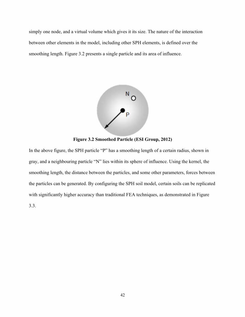
smoothing length. Figure 3.2 presents a single particle and its area of influence.
Figure 3.2 Smoothed Particle (ESI Group, 2012)
In the above figure, the SPH particle “P” has a smoothing length of a certain radius, shown in
gray, and a neighbouring particle “N” lies within its sphere of influence. Using the kernel, the
smoothing length, the distance between the particles, and some other parameters, forces between
the particles can be generated. By configuring the SPH soil model, certain soils can be replicated
with significantly higher accuracy than traditional FEA techniques, as demonstrated in Figure
3.3.
43
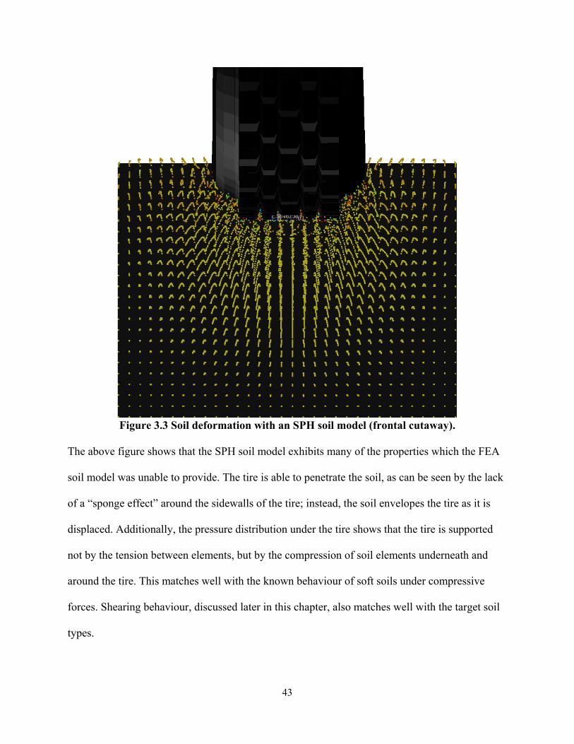
Figure 3.3 Soil deformation with an SPH soil model (frontal cutaway).
The above figure shows that the SPH soil model exhibits many of the properties which the FEA
soil model was unable to provide. The tire is able to penetrate the soil, as can be seen by the lack
of a “sponge effect” around the sidewalls of the tire; instead, the soil envelopes the tire as it is
displaced. Additionally, the pressure distribution under the tire shows that the tire is supported
not by the tension between elements, but by the compression of soil elements underneath and
around the tire. This matches well with the known behaviour of soft soils under compressive
forces. Shearing behaviour, discussed later in this chapter, also matches well with the target soil
types.

44
SPH models are developed by first creating a regular FEA solid and meshing it. For this
research, the hexahedral mesh is used to reduce the complexity of the model when converting to
SPH elements. As SPH elements inherit the volume of the source elements, it is convenient and
less computationally-intensive to work with a uniform, perfectly-aligned mesh. (El-Gindy M. L.,
2011) initially investigated the possibility of using SPH as a modeling technique for soils, and
found that it would require significant further work to get models to the stage where they could
be considered valid. However, that research provided insight for this work, as it found that it was
indeed feasible, and provided a basis for choosing the mesh size. Based on the information
gathered from that work, the initial mesh size was chosen to be uniformly 25mm, as it was found
that reducing the mesh further did not yield significant improvements in the model.
The material used for the soil models are elastic-plastic solid types corresponding to available
data on real soils. Elastic-plastic materials are not only convenient, but they also provide us with
the opportunity to compare FEA and SPH soil models as the same material type is used for the
FEA models as well. For this reason, the FEA models are developed first, then a copy is made in
order to convert the FEA elements to SPH elements using the conversion tool within the PAM-
CRASH software. Any attributes that can be retained from during the conversion process, or can
be added post-conversion, are kept so that the comparison between the two methods may be as
close as possible.
3.1.1 SPH Parameters
There are a number of SPH parameters that have an influence on the behaviour of the soil model,
apart from the material properties. The Hmin, Hmax, and RATIO variables are part of the SPH
interaction properties. Figure 3.4 shows an SPH particle and its various interaction zones.

45
Figure 3.4 An SPH particle with a RATIO value of 1.5. (ESI Group, 2012)
In the previous figure, the “r” value is determined by the source element. That is, the volume of
the element before conversion is preserved during conversion, however instead of a cube, the
element is given a spherical volume corresponding to a radius “r”. The RATIO determines the
nominal smoothing length and is the quotient of the “r” value and the “h” value; in the case of
figure Figure 3.4, it is 1.5. It is important to note that the smoothing length is not fixed. Hmin and
Hmax provide bounds for the smoothing length when particles shift, in order to maintain
cohesion. For the majority of the models in this research, Hmin is 1, Hmax is 35 and RATIO is
2.1.
The smoothing values are used in conjunction with the kernel, among other factors such as
material properties, to calculate the forces between SPH elements. The kernel parameter, called
IDKERN in the software, determines the interaction model used over the smoothing length. It
defines the influence of all neighbouring particles on the particle in question. By default, the W4
B-spline function shown in Figure 3.5 is used, where the horizontal axis is the multiple of the
smoothing length “h” and the vertical axis is the interpolation factor. This research provides
some insight into the effect of the kernel on soil behaviour as a possible area of study in future
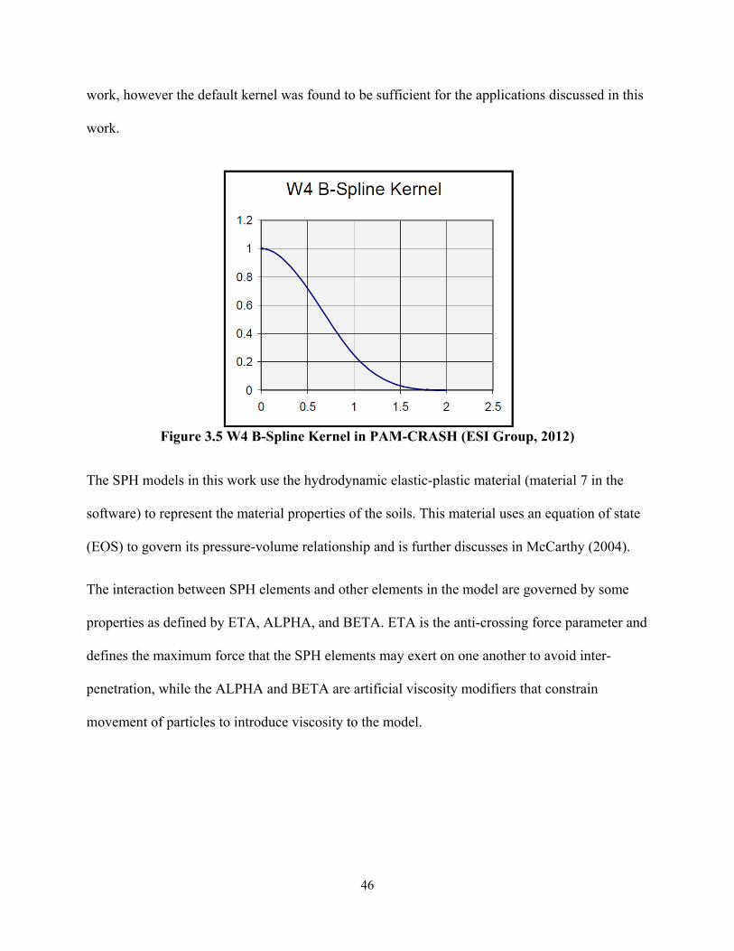
46
work, however the default kernel was found to be sufficient for the applications discussed in this
work.
Figure 3.5 W4 B-Spline Kernel in PAM-CRASH (ESI Group, 2012)
The SPH models in this work use the hydrodynamic elastic-plastic material (material 7 in the
software) to represent the material properties of the soils. This material uses an equation of state
(EOS) to govern its pressure-volume relationship and is further discusses in McCarthy (2004).
The interaction between SPH elements and other elements in the model are governed by some
properties as defined by ETA, ALPHA, and BETA. ETA is the anti-crossing force parameter and
defines the maximum force that the SPH elements may exert on one another to avoid inter-
penetration, while the ALPHA and BETA are artificial viscosity modifiers that constrain
movement of particles to introduce viscosity to the model.
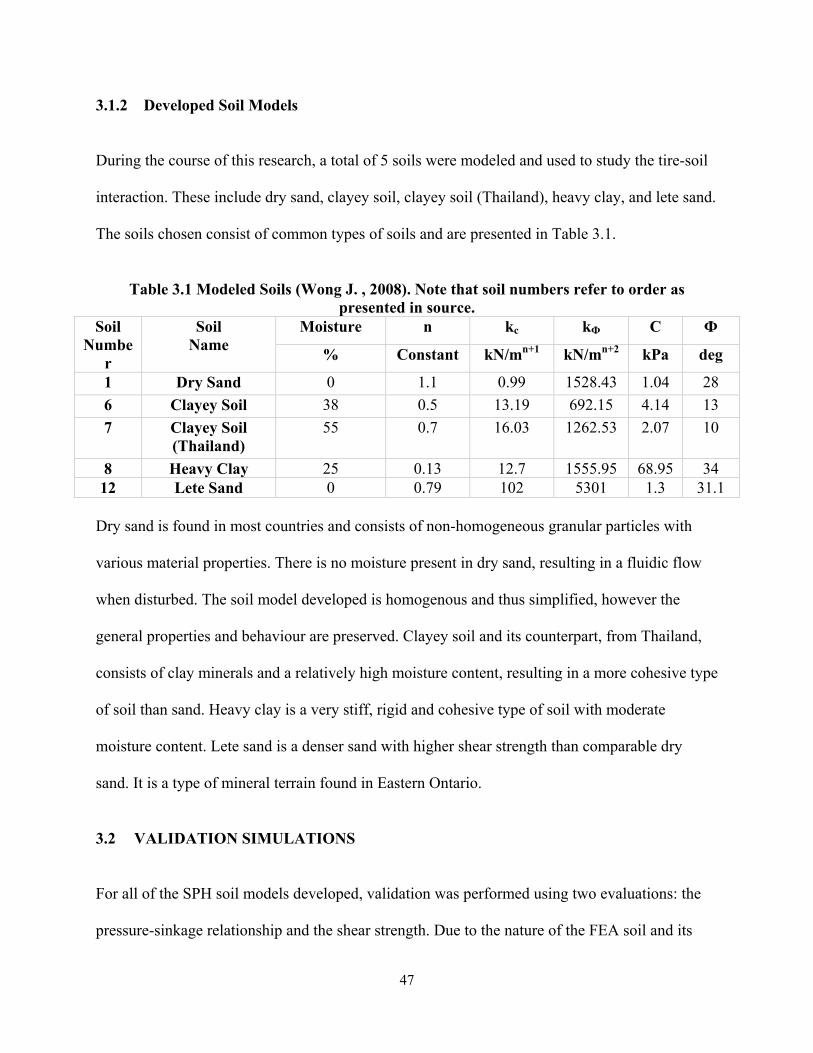
47
3.1.2 Developed Soil Models
During the course of this research, a total of 5 soils were modeled and used to study the tire-soil
interaction. These include dry sand, clayey soil, clayey soil (Thailand), heavy clay, and lete sand.
The soils chosen consist of common types of soils and are presented in Table 3.1.
Table 3.1 Modeled Soils (Wong J. , 2008). Note that soil numbers refer to order as presented in source.
Soil Numbe
r
Soil Name
Moisture n kc kФ C Ф
% Constant kN/mn+1 kN/mn+2 kPa deg
1 Dry Sand 0 1.1 0.99 1528.43 1.04 28
6 Clayey Soil 38 0.5 13.19 692.15 4.14 13
7 Clayey Soil (Thailand)
55 0.7 16.03 1262.53 2.07 10
8 Heavy Clay 25 0.13 12.7 1555.95 68.95 34 12 Lete Sand 0 0.79 102 5301 1.3 31.1
Dry sand is found in most countries and consists of non-homogeneous granular particles with
various material properties. There is no moisture present in dry sand, resulting in a fluidic flow
when disturbed. The soil model developed is homogenous and thus simplified, however the
general properties and behaviour are preserved. Clayey soil and its counterpart, from Thailand,
consists of clay minerals and a relatively high moisture content, resulting in a more cohesive type
of soil than sand. Heavy clay is a very stiff, rigid and cohesive type of soil with moderate
moisture content. Lete sand is a denser sand with higher shear strength than comparable dry
sand. It is a type of mineral terrain found in Eastern Ontario.
3.2 VALIDATION SIMULATIONS
For all of the SPH soil models developed, validation was performed using two evaluations: the
pressure-sinkage relationship and the shear strength. Due to the nature of the FEA soil and its
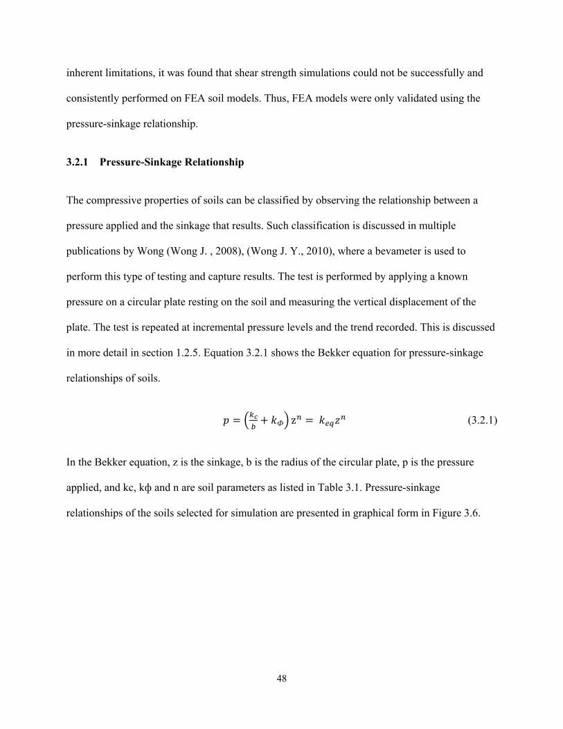
48
inherent limitations, it was found that shear strength simulations could not be successfully and
consistently performed on FEA soil models. Thus, FEA models were only validated using the
pressure-sinkage relationship.
3.2.1 Pressure-Sinkage Relationship
The compressive properties of soils can be classified by observing the relationship between a
pressure applied and the sinkage that results. Such classification is discussed in multiple
publications by Wong (Wong J. , 2008), (Wong J. Y., 2010), where a bevameter is used to
perform this type of testing and capture results. The test is performed by applying a known
pressure on a circular plate resting on the soil and measuring the vertical displacement of the
plate. The test is repeated at incremental pressure levels and the trend recorded. This is discussed
in more detail in section 1.2.5. Equation 3.2.1 shows the Bekker equation for pressure-sinkage
relationships of soils.
Ф z (3.2.1)
In the Bekker equation, z is the sinkage, b is the radius of the circular plate, p is the pressure
applied, and kc, kф and n are soil parameters as listed in Table 3.1. Pressure-sinkage
relationships of the soils selected for simulation are presented in graphical form in Figure 3.6.
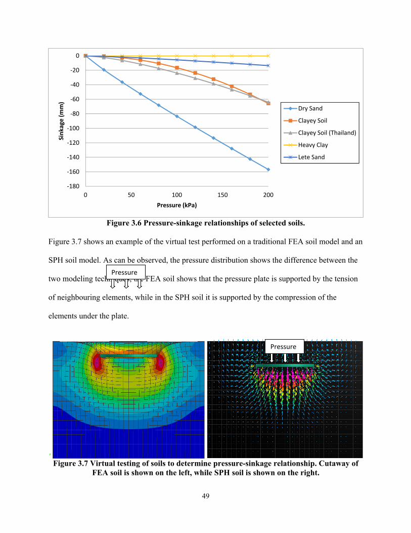
49
Figure 3.6 Pressure-sinkage relationships of selected soils.
Figure 3.7 shows an example of the virtual test performed on a traditional FEA soil model and an
SPH soil model. As can be observed, the pressure distribution shows the difference between the
two modeling techniques; the FEA soil shows that the pressure plate is supported by the tension
of neighbouring elements, while in the SPH soil it is supported by the compression of the
elements under the plate.
Figure 3.7 Virtual testing of soils to determine pressure-sinkage relationship. Cutaway of
FEA soil is shown on the left, while SPH soil is shown on the right.
‐180
‐160
‐140
‐120
‐100
‐80
‐60
‐40
‐20
0
0 50 100 150 200
Sinkage (mm)
Pressure (kPa)
Dry Sand
Clayey Soil
Clayey Soil (Thailand)
Heavy Clay
Lete Sand
Pressure
Pressure

50
3.2.2 Shear Strength
The shear properties of a soil are essential to studying the interaction between soft terrain and
tires. Unlike on road surfaces, where most of the longitudinal slip in a tire’s motion is due to
tread flexure, on soft soils the slip is largely attributed to the shearing of soil layers, causing the
vehicle to experience reduced traction as the tires displace the terrain.
In this research, shear strength of soils is classified using the Mohr-Coulomb failure criterion.
The shear strength validations were performed using the direct shear method, or commonly
known as the shear box test. The test consists of constraining a soil within a box with fixed walls
and bottom, and then placing a loading plate on the top of the open box. The plate can then be
loaded to various vertical loads. The test is performed by separating two halves of the box at the
middle horizontal plane by applying a fixed displacement, and then measuring the force
generated in the shearing direction. The yield is represented by the point at which resistive force
decreases or levels off after the peak. The shear strength can be calculated from the force
readings by dividing the force by the cross-sectional area of the shear box.
It is important to note that the shear box test, though widely used to collect experimental data, is
not an absolute method for obtaining shear properties of soils. As stated in (Poulos, 1989), the
shear strength is affected by many factors, such as soil composition (homogenous, moisture,
etc.), initial state (compressed, free, etc.), structure and loading conditions. Further, it is clear that
the shear strength versus vertical load relationship is not linear. The actual data, both from
experiments and from the virtual simulations performed for this report, shows that it is actually a
curve, however for approximation a linear best-fit line is used to represent the shear properties.
The shear box created in PAM CRASH for shear strength tests has a cross sectional area of 0.15
m2 and is moved to a distance of 200 mm over the course of 1 second, after vertically loading
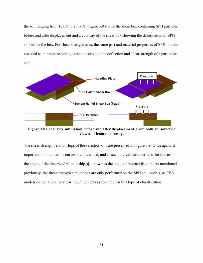
51
the soil ranging from 10kPa to 200kPa. Figure 3.8 shows the shear box containing SPH particles
before and after displacement and a cutaway of the shear box showing the deformation of SPH
soil inside the box. For shear strength tests, the same part and material properties of SPH models
are used as in pressure-sinkage tests to correlate the deflection and shear strength of a particular
soil.
Figure 3.8 Shear box simulation before and after displacement, from both an isometric
view and frontal cutaway.
The shear strength relationships of the selected soils are presented in Figure 3.9. Once again, it
important to note that the curves are linearized, and as such the validation criteria for this test is
the angle of the linearized relationship, ф ,known as the angle of internal friction. As mentioned
previously, the shear strength simulations are only performed on the SPH soil models, as FEA
models do not allow for shearing of elements as required for this type of classification.
Pressure
Pressure
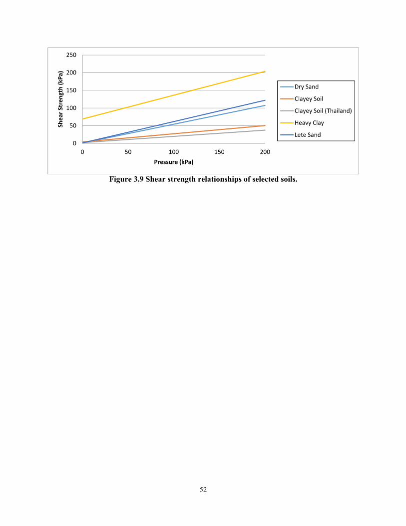
52
Figure 3.9 Shear strength relationships of selected soils.
0
50
100
150
200
250
0 50 100 150 200
Shear Strength (kPa)
Pressure (kPa)
Dry Sand
Clayey Soil
Clayey Soil (Thailand)
Heavy Clay
Lete Sand

53
CHAPTER 4: SIMULATIONS ON HARD SURFACES
Hard surface simulations were performed using the 3-groove pneumatic tire model developed
earlier in this research. Once validated, the models was subjected to a number of simulations
including simple rolling resistance simulations, quarter-vehicle model simulations on rough
roads, as well as slip and camber simulations to capture steering characteristics of the tire.
4.1 ROLLING RESISTANCE SIMULATIONS
The rolling resistance simulations were performed with a full tire and wheel model placed on a
virtual road of the same type (rigid body) as the surface for the static deflection simulations. The
surface was lengthened to 100 meters and applied a constant velocity in the longitudinal tire axis,
while the wheel is restricted to movement in the z-axis and rotation along the y-axis only. Thus,
the tire is allowed to roll freely and the forces in the longitudinal and vertical direction may be
measured to determine rolling resistance. The complete simulation model is shown in Figure 4.1.
Figure 4.1 The complete model for determining the rolling resistance of the FEA tire. The
arrow indicates the direction of road velocity relative to the free-rolling tire and wheel assembly.
The various operating parameters that effect rolling resistance, and which are investigated in the
simulations, are the inflation pressure, vertical load, vehicle speed and the road friction
coefficient. Table 4.1 presents the complete simulation parameters.
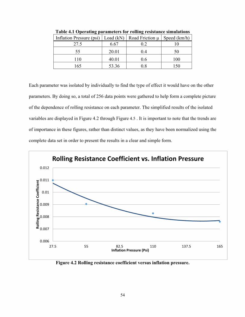
54
Table 4.1 Operating parameters for rolling resistance simulations Inflation Pressure (psi) Load (kN) Road Friction µ Speed (km/h)
27.5 6.67 0.2 10
55 20.01 0.4 50
110 40.01 0.6 100
165 53.36 0.8 150
Each parameter was isolated by individually to find the type of effect it would have on the other
parameters. By doing so, a total of 256 data points were gathered to help form a complete picture
of the dependence of rolling resistance on each parameter. The simplified results of the isolated
variables are displayed in Figure 4.2 through Figure 4.5 . It is important to note that the trends are
of importance in these figures, rather than distinct values, as they have been normalized using the
complete data set in order to present the results in a clear and simple form.
Figure 4.2 Rolling resistance coefficient versus inflation pressure.
0.006
0.007
0.008
0.009
0.01
0.011
0.012
27.5 55 82.5 110 137.5 165
Rolling Resistan
ce Coefficient
Inflation Pressure (Psi)
Rolling Resistance Coefficient vs. Inflation Pressure

55
Figure 4.3 Rolling resistance coefficient versus translational speed (of center of tire
spindle).
Figure 4.4 Rolling resistance coefficient versus road friction coefficient.
0
0.005
0.01
0.015
0.02
0.025
0.03
0 25 50 75 100 125 150
Rolling Resistan
ce Coefficient
Speed (Kph)
Rolling Resistance Coefficient vs. Speed
0.00813
0.00816
0.00819
0.00822
0.00825
0.00828
0.00831
0.2 0.3 0.4 0.5 0.6 0.7 0.8
Rolling Resistan
ce Coefficient
Road Friction Coefficient
Rolling Resistance Coefficient vs. Road Friction Coefficient
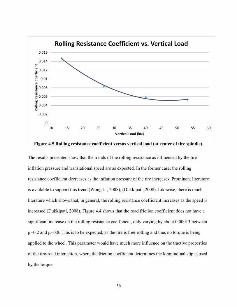
56
Figure 4.5 Rolling resistance coefficient versus vertical load (at center of tire spindle).
The results presented show that the trends of the rolling resistance as influenced by the tire
inflation pressure and translational speed are as expected. In the former case, the rolling
resistance coefficient decreases as the inflation pressure of the tire increases. Prominent literature
is available to support this trend (Wong J. , 2008), (Dukkipati, 2008). Likewise, there is much
literature which shows that, in general, the rolling resistance coefficient increases as the speed is
increased (Dukkipati, 2008). Figure 4.4 shows that the road friction coefficient does not have a
significant increase on the rolling resistance coefficient, only varying by about 0.00013 between
µ=0.2 and µ=0.8. This is to be expected, as the tire is free-rolling and thus no torque is being
applied to the wheel. This parameter would have much more influence on the tractive properties
of the tire-road interaction, where the friction coefficient determines the longitudinal slip caused
by the torque.
0
0.002
0.004
0.006
0.008
0.01
0.012
0.014
0.016
10 15 20 25 30 35 40 45 50 55 60
Rolling Resistan
ce Coefficient
Vertical Load (kN)
Rolling Resistance Coefficient vs. Vertical Load
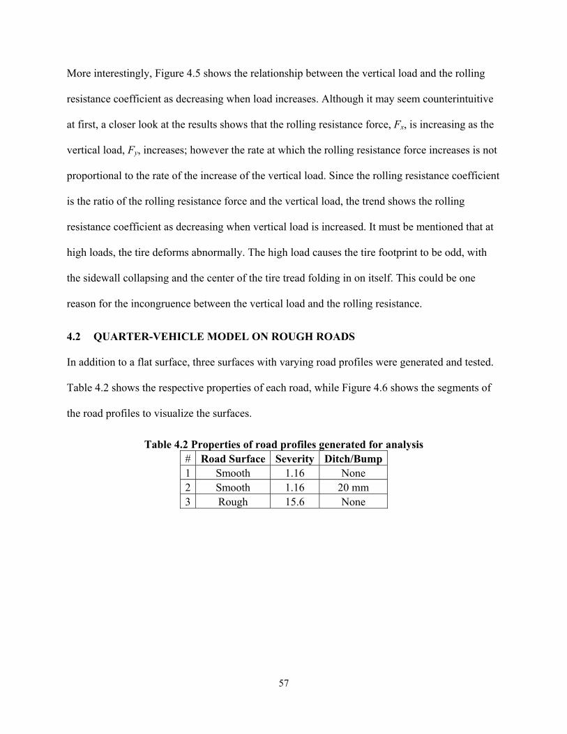
57
More interestingly, Figure 4.5 shows the relationship between the vertical load and the rolling
resistance coefficient as decreasing when load increases. Although it may seem counterintuitive
at first, a closer look at the results shows that the rolling resistance force, Fx, is increasing as the
vertical load, Fy, increases; however the rate at which the rolling resistance force increases is not
proportional to the rate of the increase of the vertical load. Since the rolling resistance coefficient
is the ratio of the rolling resistance force and the vertical load, the trend shows the rolling
resistance coefficient as decreasing when vertical load is increased. It must be mentioned that at
high loads, the tire deforms abnormally. The high load causes the tire footprint to be odd, with
the sidewall collapsing and the center of the tire tread folding in on itself. This could be one
reason for the incongruence between the vertical load and the rolling resistance.
4.2 QUARTER-VEHICLE MODEL ON ROUGH ROADS
In addition to a flat surface, three surfaces with varying road profiles were generated and tested.
Table 4.2 shows the respective properties of each road, while Figure 4.6 shows the segments of
the road profiles to visualize the surfaces.
Table 4.2 Properties of road profiles generated for analysis # Road Surface Severity Ditch/Bump1 Smooth 1.16 None 2 Smooth 1.16 20 mm 3 Rough 15.6 None
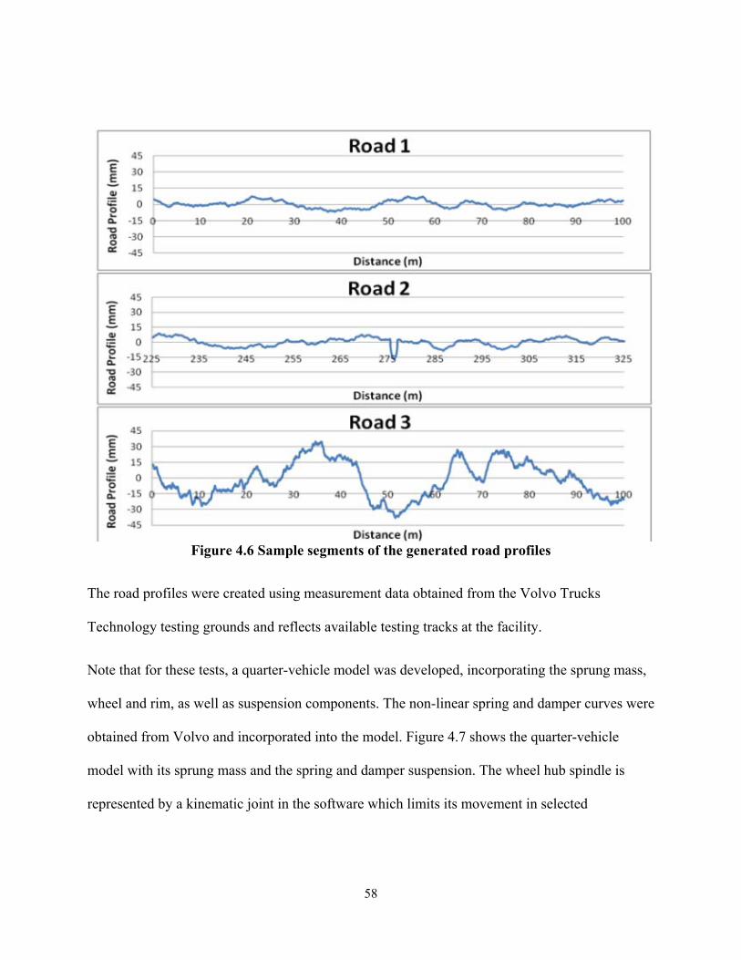
58
Figure 4.6 Sample segments of the generated road profiles
The road profiles were created using measurement data obtained from the Volvo Trucks
Technology testing grounds and reflects available testing tracks at the facility.
Note that for these tests, a quarter-vehicle model was developed, incorporating the sprung mass,
wheel and rim, as well as suspension components. The non-linear spring and damper curves were
obtained from Volvo and incorporated into the model. Figure 4.7 shows the quarter-vehicle
model with its sprung mass and the spring and damper suspension. The wheel hub spindle is
represented by a kinematic joint in the software which limits its movement in selected
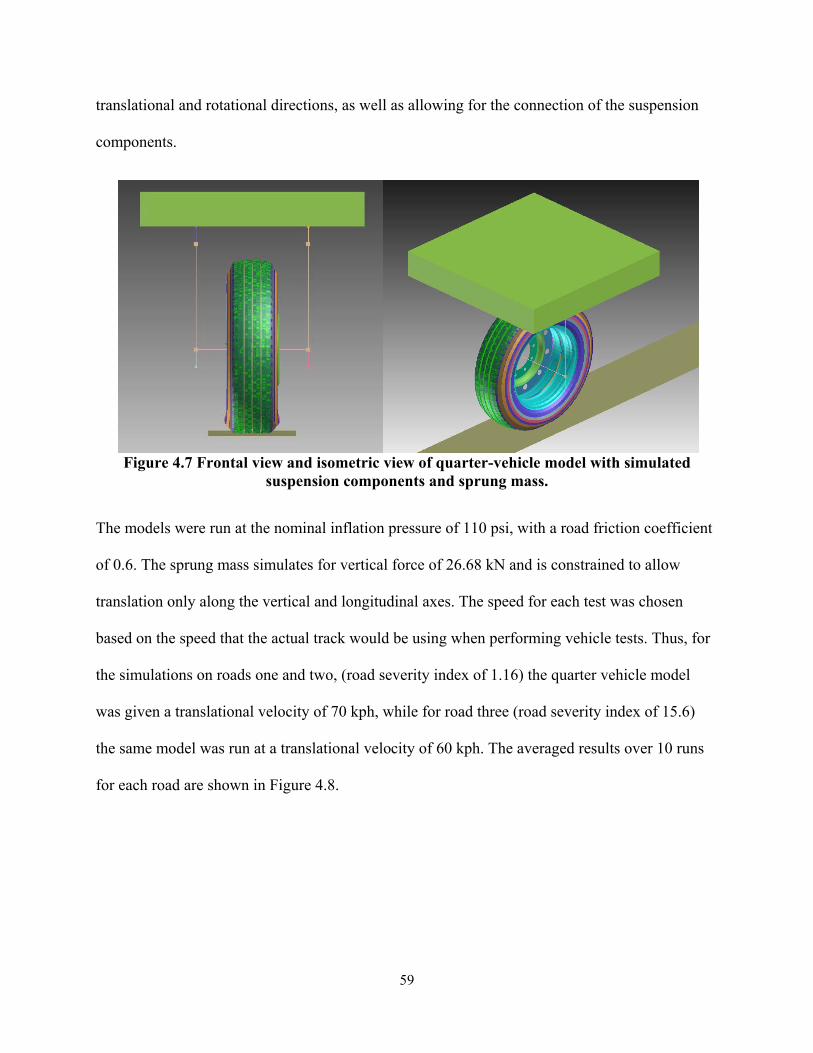
59
translational and rotational directions, as well as allowing for the connection of the suspension
components.
Figure 4.7 Frontal view and isometric view of quarter-vehicle model with simulated
suspension components and sprung mass.
The models were run at the nominal inflation pressure of 110 psi, with a road friction coefficient
of 0.6. The sprung mass simulates for vertical force of 26.68 kN and is constrained to allow
translation only along the vertical and longitudinal axes. The speed for each test was chosen
based on the speed that the actual track would be using when performing vehicle tests. Thus, for
the simulations on roads one and two, (road severity index of 1.16) the quarter vehicle model
was given a translational velocity of 70 kph, while for road three (road severity index of 15.6)
the same model was run at a translational velocity of 60 kph. The averaged results over 10 runs
for each road are shown in Figure 4.8.

60
Figure 4.8 Rolling resistance coefficient over various road surfaces.
The results show that compared with the perfectly flat road, roads one and two exhibited 6.3%
and 7.8% higher rolling resistance coefficients, respectively. The introduction of potholes and
bumps caused the rolling resistance coefficient to increase by a further 1.35% even though the
roads were identical otherwise. The rough road, road three, showed an increase of 8.91% in the
rolling resistance coefficient in comparison with the perfectly flat road profile.
4.3 STEERING CHARACTERISTICS
The slip and camber angle simulations were performed on a perfectly flat surface. For these
simulations, the tire model was rotated along the appropriate axis relative to the direction of
motion, and then lowered on to the virtual road surface. A load was applied at the center of the
model’s spindle and the tire model was allowed to rotate along the y-axis and translate in the z-
direction only. Figure 4.9 and Figure 4.10 show the orientation of the wheel assembly when
camber and slip angles are applied.
0.0056278
0.0060648
0.006449
0.006536
0.006129
0.005 0.0052 0.0054 0.0056 0.0058 0.006 0.0062 0.0064 0.0066
Flat (60 kph)
Flat (70 kph)
Road 1 (70 kph)
Road 2 (70 kph)
Road 3 (60 kph)
Note: Tire velocity for Roads 1 and 2 is 70 kph. Tire velocity for Road 3 is 60 kph. Road 3 represents an extreme case due to large variations in surface texture. Tire inflation pressure is 110 psi; tire load is 26.68 kN; road friction coefficient µ=0.6
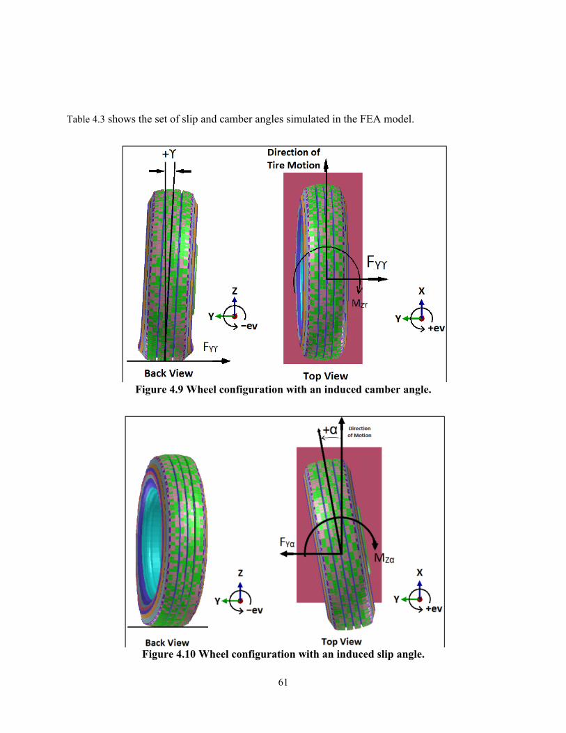
61
Table 4.3 shows the set of slip and camber angles simulated in the FEA model.
Figure 4.9 Wheel configuration with an induced camber angle.
Figure 4.10 Wheel configuration with an induced slip angle.
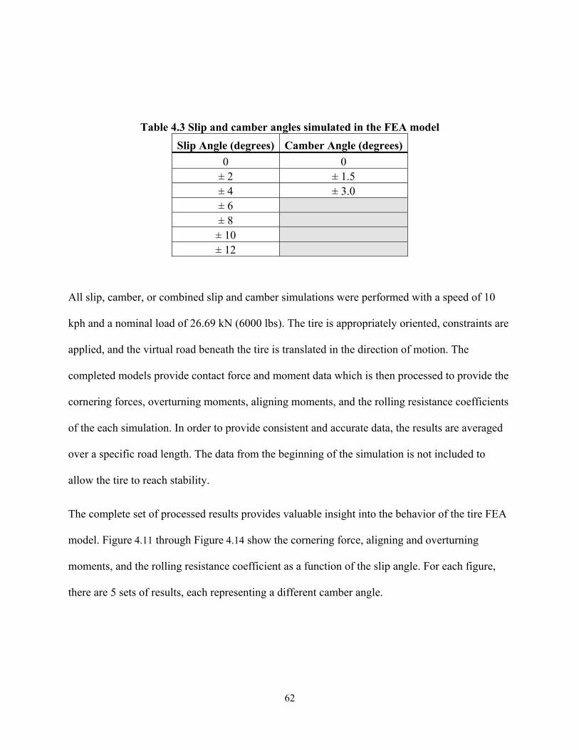
62
Table 4.3 Slip and camber angles simulated in the FEA model
Slip Angle (degrees) Camber Angle (degrees)
0 0 ± 2 ± 1.5 ± 4 ± 3.0 ± 6 ± 8 ± 10 ± 12
All slip, camber, or combined slip and camber simulations were performed with a speed of 10
kph and a nominal load of 26.69 kN (6000 lbs). The tire is appropriately oriented, constraints are
applied, and the virtual road beneath the tire is translated in the direction of motion. The
completed models provide contact force and moment data which is then processed to provide the
cornering forces, overturning moments, aligning moments, and the rolling resistance coefficients
of the each simulation. In order to provide consistent and accurate data, the results are averaged
over a specific road length. The data from the beginning of the simulation is not included to
allow the tire to reach stability.
The complete set of processed results provides valuable insight into the behavior of the tire FEA
model. Figure 4.11 through Figure 4.14 show the cornering force, aligning and overturning
moments, and the rolling resistance coefficient as a function of the slip angle. For each figure,
there are 5 sets of results, each representing a different camber angle.
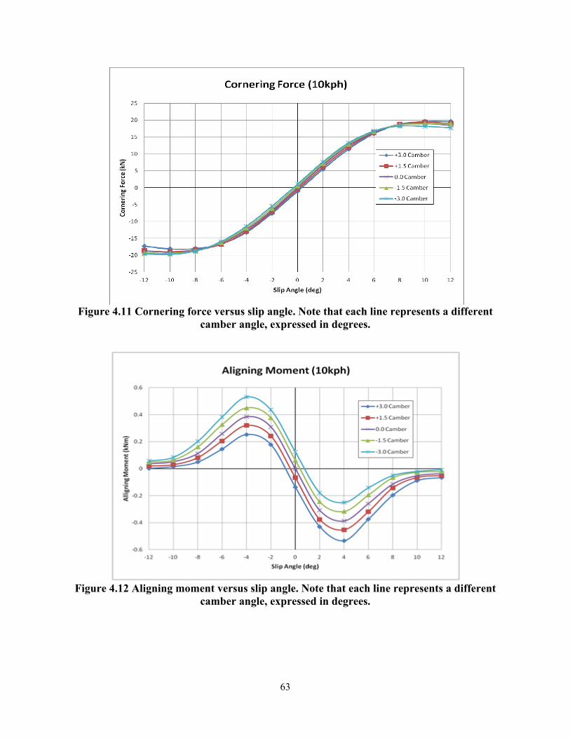
63
Figure 4.11 Cornering force versus slip angle. Note that each line represents a different
camber angle, expressed in degrees.
Figure 4.12 Aligning moment versus slip angle. Note that each line represents a different
camber angle, expressed in degrees.

64
Figure 4.13 Overturning moment versus slip angle. Note that each line represents a
different camber angle, expressed in degrees.
Figure 4.14 Rolling resistance coefficient versus slip angle. Note that each line represents a
different camber angle, expressed in degrees.
There is little variance of the cornering force due to the camber angle, however the slip angle
shows a large influence in the preceding figures. It is much more apparent that the camber angle
has a heavy influence in the aligning and overturning moments. These trends are not surprising,
since inducing a camber angle changes the geometry of the tire-ground interaction and results in

65
the large change in the moments. Not only are the results intuitively correct, but they are verified
to be in good correlation with actual measurements from a comparable tire (El-Gindy M. C.,
2001). Pacejka (Pacejka H. B., 1997) presents a “Magic Formula” tire model, which aims to
simplify the estimation of the side forces as well as aligning and overturning moments. The data
presented in this chapter was found to conform to the trends seen in the Magic Formula in each
case. The Magic Formula is a model derived from experimental data and adapted to specific
tires. It is widely considered to be a reliable source of qualitative relationships between the
various factors affecting tire performance.
The rolling resistance is seen to have a large dependence on the slip angle, however the effect of
camber is only prominent at very large slip angles, where the simulations show divergence
between the data sets.

66
CHAPTER 5: SIMULATIONS ON SOFT SOILS
Simulations on soils modeled and validated in Chapter 3 were performed using the Regional
Haul Drive (RHD) tire discussed in section 2.3. The simulations focus on obtaining the effect of
soft soils on the rolling resistance of tires. Further, the soils modeled using the traditional finite
element method are compared to the equivalent smoothed particle hydrodynamics models.
5.1 SIMULATION PROCEDURE
The general setup of the rolling resistance simulations on soft soils consists of creating a box of
virtual soil and running a free-rolling tire model over the length of it. The depth and width of the
box of soil is chosen so that the dimensions of the box have a minimal influence on the
behaviour of the soil. The length of the box was chosen to allow the tire and soil to reach a
steady state of rolling. By doing so, the beginning of the simulation, where the tire is first
dropped onto the soil and faces the largest resistance to forward movement due to the
compaction of soil around it, may be excluded from the results. This allows for analysis of the
tire-soil interaction while minimizing the influence of other factors.
The box created for the simulations is of the same material as the box used for the pressure-
sinkage validation simulations; both were created as rigid bodies and the soil-box contact allows
for the soil to remain within the boundaries of the box. The wheel assembly is placed just a few
millimetres above the soil, and once the simulation begins, the tire is inflated and the wheel
assembly is lowered onto the soil. Gravity is accounted for using an acceleration field. Once the
tire and soil have settled, the tire model is assigned a translational velocity of 10 kph (2.78 m/s)
at the tire spindle in the x-direction. The box of soil is fully fixed, while the wheel assembly is

67
constrained so that vertical and longitudinal translation, as well as rotation along the tire spindle
(y-axis) is allowed.
Once a simulation is completed, results are obtained by collecting the data from the contact
between the tire and the soil elements. A complete model of the RHD tire rolling over SPH soil
is shown in Figure 5.1 with the box enclosing the soil hidden.
Figure 5.1 Free rolling tire on SPH soil.
The rolling resistance coefficient is calculated by finding the ratio of the resistive force in the
longitudinal direction (x-direction in the model) and the vertical load on the tire. Both the
vertical load as well as the tire inflation pressure were varied to find each factor’s effect on the
rolling resistance over the various soft soils. Table 5.1 shows the complete set of parameters for
rolling resistance simulations on soft soils.

68
Table 5.1 Operating parameters for rolling resistance simulations on soft soils Inflation Pressure (psi) Load (kN, lbs) Speed (km/h)
55 6.67, 1500 10
110 13.34, 3000
165 26.68, 1600
5.2 ROLLING RESISTANCE SIMULATION RESULTS
This section presents the results of the rolling resistance simulations on soft soils, presented and
validated in Chapter 3. Each soil was modeled using traditional FEA, as well as SPH techniques
in order to compare the variation in the results, as well as determine the feasibility of each type
of soil model. Figures Figure 5.2 through Figure 5.11 show the results of each type of soil with
respect to tire inflation pressure and vertical load. It is important to note that the curves fitted to
the data in these figures do not encompass the complete set of data available, but were chosen to
capture the trends seen in the larger data sets. Furthermore, the data has been filtered to remove
noise and excessive variations.
5.2.1 Dry Sand
Figure 5.2 Rolling resistance coefficient versus tire inflation pressure on dry sand.

69
Figure 5.3 Rolling resistance coefficient versus vertical load on dry sand.
5.2.2 Clayey Soil
Figure 5.4 Rolling resistance coefficient versus tire inflation pressure on clayey soil.

70
Figure 5.5 Rolling resistance coefficient versus vertical load on clayey soil.
5.2.3 Clayey Soil (Thailand)
Figure 5.6 Rolling resistance coefficient versus tire inflation pressure on clayey soil
(Thailand).
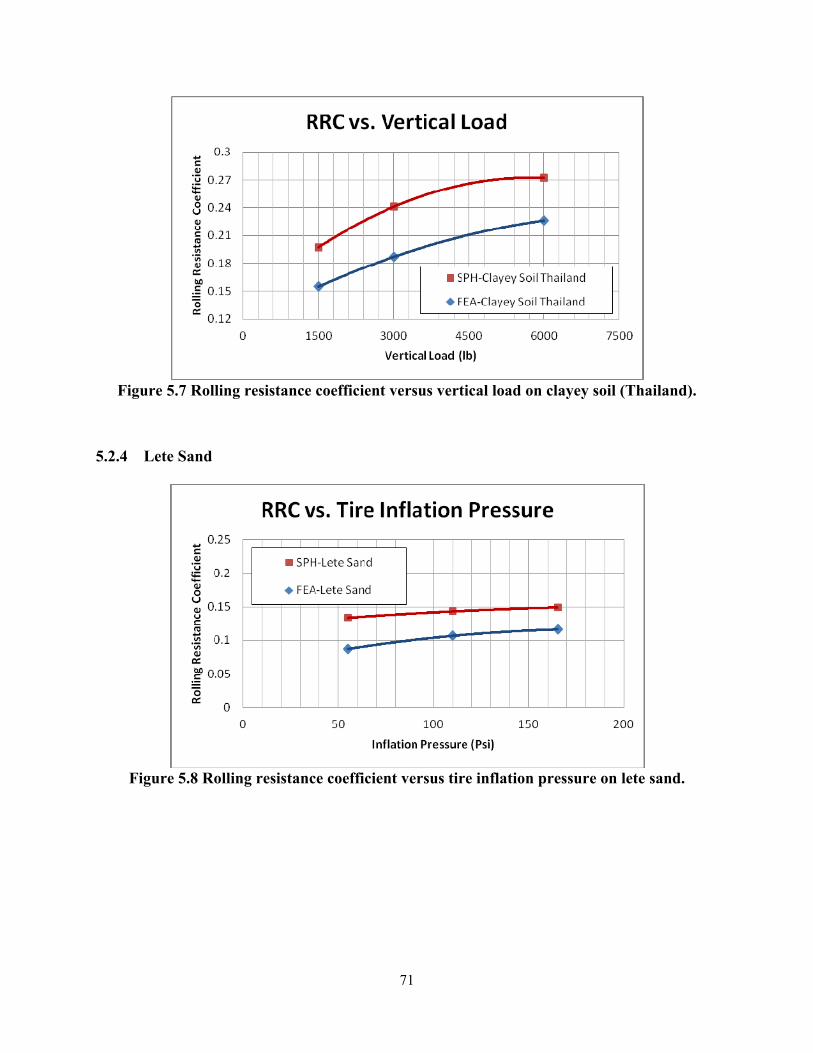
71
Figure 5.7 Rolling resistance coefficient versus vertical load on clayey soil (Thailand).
5.2.4 Lete Sand
Figure 5.8 Rolling resistance coefficient versus tire inflation pressure on lete sand.
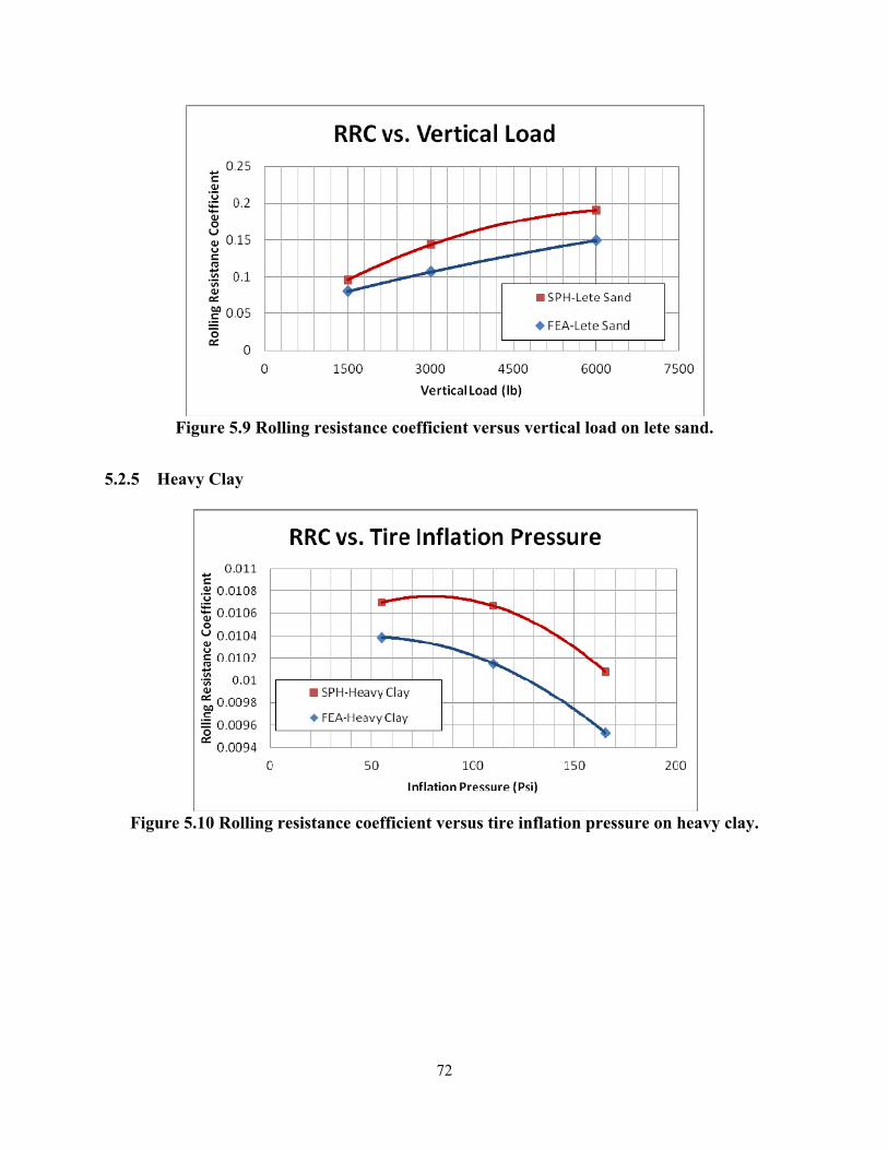
72
Figure 5.9 Rolling resistance coefficient versus vertical load on lete sand.
5.2.5 Heavy Clay
Figure 5.10 Rolling resistance coefficient versus tire inflation pressure on heavy clay.

73
Figure 5.11 Rolling resistance coefficient versus vertical load on heavy clay.
5.3 SUMMARY
The results of the rolling resistance simulations on FEA and SPH soil models show some notable
trends. In particular, it can be noted that the SPH soil model exhibited many behaviours which
differentiate it from the equivalent FEA soil model.
The limitations inherent to the finite element method cause the rolling resistance to be generally
lower than the same soil when represented with SPH elements. Figure 5.12 shows a comparison
of the FEA and SPH simulations on clayey soil (Thailand). It must be noted that the simulation is
at the same location and timestep for both captures. At this point, the tire is rolling at a speed of
10 kph over the soil and it is about 3 meters into the box.
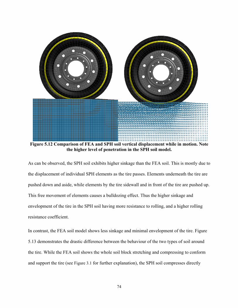
74
Figure 5.12 Comparison of FEA and SPH soil vertical displacement while in motion. Note
the higher level of penetration in the SPH soil model.
As can be observed, the SPH soil exhibits higher sinkage than the FEA soil. This is mostly due to
the displacement of individual SPH elements as the tire passes. Elements underneath the tire are
pushed down and aside, while elements by the tire sidewall and in front of the tire are pushed up.
This free movement of elements causes a bulldozing effect. Thus the higher sinkage and
envelopment of the tire in the SPH soil having more resistance to rolling, and a higher rolling
resistance coefficient.
In contrast, the FEA soil model shows less sinkage and minimal envelopment of the tire. Figure
5.13 demonstrates the drastic difference between the behaviour of the two types of soil around
the tire. While the FEA soil shows the whole soil block stretching and compressing to conform
and support the tire (see Figure 3.1 for further explanation), the SPH soil compresses directly

75
underneath the centerline of the tire, but elements to the left or right displace and move the
surrounding soil out and up.
Figure 5.13 Cut-away of tire while rolling on clayey soil (Thailand).
When compared to the available experimental data, the rolling resistance predicted using both
the FEA as well as the SPH models followed the expected trends. However, the SPH models
proved to be more accurate quantitatively, as the predicted rolling resistance coefficients were
generally closer to or within the ranges provided by experimental data. Figure 5.14 shows a
summary of some types of soils and the expected change in the rolling resistance coefficient with
variation of tire inflation pressure. It shows that softer soils such as sand, and particularly sands
with less moisture, will exhibit a large increase in the rolling resistance coefficient as the
inflation pressure is increased, mainly due to the increased rigidity of the tire and higher sinkage

76
(Wong J. Y., 2010). This trend is seen in all of the modeled soils except heavy clay. Increasing
the load also causes higher sinkage of the tire into the soil, as well as increased flexure of the
sidewall, both of which cause rolling resistance to increase.
Figure 5.14 Variation of rolling resistance coefficient with inflation pressure of tires on
various surfaces. Source: (Wong J. , 2008)
The data shows that, as with a rigid surface such as concrete, increasing the inflation pressure
causes the rolling resistance coefficient to decrease on harder soils. Once again, this is due to the
increased rigidity of the tire, resulting in less flexure in the sidewall and lower rolling resistance.
Since harder soils allow less sinkage and envelopment of the tire, this results in a lower rolling
resistance coefficient. The decrease of the rolling resistance coefficient due to increased load on
harder soils (heavy clay) is explained in section 4.1.
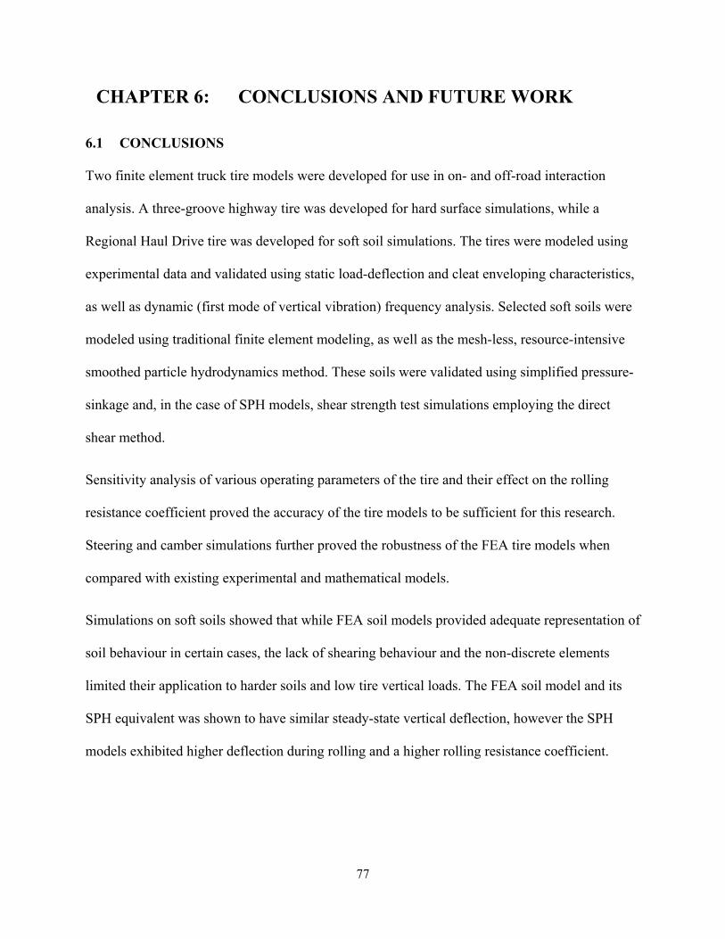
77
CHAPTER 6: CONCLUSIONS AND FUTURE WORK
6.1 CONCLUSIONS
Two finite element truck tire models were developed for use in on- and off-road interaction
analysis. A three-groove highway tire was developed for hard surface simulations, while a
Regional Haul Drive tire was developed for soft soil simulations. The tires were modeled using
experimental data and validated using static load-deflection and cleat enveloping characteristics,
as well as dynamic (first mode of vertical vibration) frequency analysis. Selected soft soils were
modeled using traditional finite element modeling, as well as the mesh-less, resource-intensive
smoothed particle hydrodynamics method. These soils were validated using simplified pressure-
sinkage and, in the case of SPH models, shear strength test simulations employing the direct
shear method.
Sensitivity analysis of various operating parameters of the tire and their effect on the rolling
resistance coefficient proved the accuracy of the tire models to be sufficient for this research.
Steering and camber simulations further proved the robustness of the FEA tire models when
compared with existing experimental and mathematical models.
Simulations on soft soils showed that while FEA soil models provided adequate representation of
soil behaviour in certain cases, the lack of shearing behaviour and the non-discrete elements
limited their application to harder soils and low tire vertical loads. The FEA soil model and its
SPH equivalent was shown to have similar steady-state vertical deflection, however the SPH
models exhibited higher deflection during rolling and a higher rolling resistance coefficient.
78
6.2 RECOMMENDATIONS FOR FUTURE WORK
The soil models employed in this research show the potential of using smoothed particle
hydrodynamics elements for material strength models, more specifically particulate materials
such as soft soils. The hydrodynamic elastic-plastic SPH material model (material type 7 in the
software) has its limitations and they have been exhibited in the course of this work. The soils
modeled are generally viscous and cohesive, and thus the particular models developed are best
suited for clayey soils. Initial use of the PAM-OPT multi-objective optimization software shows
promise of further improving the models for better matching of shear strength with experimental
data.
The Murnaghan Equation of State Solid (material type 28 in the software) has been used to
represent liquids such as water, however it should be explored as a possible material for future
modeling of non-viscous soils. Initial research into this material has shown much improved
matching of shearing properties with certain soils, however compressive properties of the soils
are difficult to match as the material does not support loads well in pressure-sinkage tests.
Limitations on time, as well as the scope of this thesis, prevented the investigation needed into
this material type, however it could prove to be ideal for representation of certain soils.
Investigation into a combination of FEA and SPH soil models is needed. Combining both types
of soils models, with the FEA on the bottom and SPH on the top surface, would reduce the
computational cost of the models. The FEA soil on the bottom does not experience significant
shear, and thus would have minimal impact on the overall results when combined with the
correct SPH model.
Future research into the behaviour of tires on soils should include camber and steering
simulations, as well as quarter-vehicle models. Soils need to be validated using data collected in

79
the field, and specific soils should be modeled using the collected data rather than the general
trends and ranges which are targeted in this research. Validation of the tire-soil interactions, as
well as the rolling resistance predictions using the various models, must be performed to
determine the accuracy and precision of the models.
80
REFERENCES
Alkan, V. K. (2011). Finite Element Modeling of Static Tire Enveloping Characteristics. International Journal of Automotive Technology, 12(4), 529-535.
Bekker, M. G. (1960). Off-the-Road Locomotion. Ann Arbor, MI: The University of Michigan Press.
Bui, H. H. (2007). Numerical Simulation of Soil-Water Interaction Using Smoothed Particle Hydrodynamics (SPH) Method. Journal of Terramechanics, 44, 339-346.
Bui, H. H. (2008). Lagrangian Meshfree Particles Method (SPH) for Large Deformation and Failure Flows of Geomaterial using Elastic-Plastic Soil Constitutive Model. International Journal for Numerical and Analytical Methods in Geomechancis, 32, 1537-1570.
Captain, K. M. (1979). Analytical Tire Models for Vehicle Dynamic Simulation. Vehicle System Dynamics, 8.
Chae, S. (2006). Nonlinear Finite Element Modeling and Analysis of a Truck Tire. University Park, PA: The Pennsylvania State University.
Chae, S. E.-G. (2001). Standing Wave Prediction of a Racing Car Tire. CSME-MDE-2001. Montreal.
Chae, S. E.-G. (2004). Dynamic Response Predictions of a Truck Tire Using Detailed Finite Element and Rigid Ring Models. 2004 ASME International Mechanical Engineering Congress and Exposition. California.
Chang, Y. P.-G. (2002). FEA Rotating Tire Modeling for Transient Response Simulation. 2002 ASME International Mechanical Engineering Congress & Exposition. New Orleans.
Cremers, R. (2005). Investigating Dynamic Tyre Model Behaviour. Eindhoven, The Netherlands: Eindhoven University of Technology.
Davis, D. C. (1974). A Radial-Spring Terrain-Enveloping Tire Model. Vehicle System Dynamics, 3.
Dukkipati, R. V. (2008). Road Vehicle Dynamics. Warrendale: SAE International.
El-Gindy, M. C. (2001). Examination of Steering Wheel Lateral Saturation of DaimlerChrysler Transport Trucks. The Pennsylvania State University.
El-Gindy, M. L. (2011). Soil Modeling using FEA and SPH Techniques for a Tire-Soil Interaction. ASME International Design Engineering Technical Conference. Washington, DC.
ESI Group. (2012). Explicit Solver Notes Manual. Paris, France: ESI Group.
81
Fitch, J. W. (1994). Motor Truck Engineering Handbook. Warrendale: Society of Automotive Engineers.
Ford, T. L. (1988). Heavy Duty Truck Tire Engineering. SAE Technical Paper 880001.
Heisler, H. (2002). Advanced Vehicle Technology. Oxford: Butterworth-Heinemann Ltd.
International Organization for Standardization. (2009). Passenger Car, Truck and Bus Tyres - Methods of Measuring Rolling Resistance - Single Point Test and Correlation of Measurement Results. ISO 28580:2009.
Janosi, Z. H. (1961). The Analytical Determination of Drawbar Pull as a Function of Slip, for Tracked Vehicles on Deformable Soils. 1st International Conference on Terrain-Vehicle Systems. Turin, Italy.
Johnson, A. F. (2006). Numerical Prediction of Damage in Composite Structures from Soft Body Impacts. Springer Science+Business Media, LLC.
Kang, N. (2009). Prediction of Tire Natural Frequency with Consideration of the Enveloping Property. International Journal of Automotive Technology, 10(1), 65-71.
Kao, B. G. (1997). Tire Transient Analysis with an Explicit Finite Element Program. Tire Science and Technology, 25(4), 230-244.
Loo, M. (1985). A Model Analysis of Tire Behavior Under Vertical Loading and Straight-Line Free Rolling. Tire Science and Technology, 13(2), 67-90.
McCarthy, M. A. (2004). Modelling of Bird Strike on an Aircraft Wing Leading Edge Made from Fibre Metal Laminates - Part 2. Applied Composite Materials, 11, 317-340.
Michelin AG. (2012, January 16). Bias vs Radial Technology. Retrieved from Michelin AG: http://www.michelinag.com/Innovating/Radial-vs.-Bias-technology
Nakajima, Y. P. (1986). Numerical Simulation of Tire Sliding Events Involving Impacts with Holes and Bumps. Tire Science and Technology, 14(2), 125-136.
Osman, M. S. (1964). The Measurement of Soil Shear Strength. Journal of Terramechanics, 1, 54-60.
Pacejka, H. B. (1997). Magic Formula Tire Model with Transient Properties. Second International Colloquium on Tire Models for Vehicle Dynamic Analysis, (pp. 234-249).
Pacejka, H. B. (2006). Tire and Vehicle Dynamics. Warrendale: SAE International.
Poulos, S. J. (1989). Liquefaction Related Phenomena. Advance Dam Engineering for Design (Van Nostrand Reinhold), 292-320.
Rakah, H. L. (2001). Vehicle Dynamics Model for Predicting Maximum Truck Acceleration Levels. Journal of Transportation Engineering, 127(5), 418-425.

82
Reece, A. R. (1965). Principles of Soil-Vehicle Mechanics. Institution of Mechanical Engineers 180 Part 2A 2.
SAE International. (2000). Rolling Resistance Measurement Procedure for Passenger Car, Light Truck, and Highway Truck and Bus Tires. SAE International.
SAE International. (2005). Tire Quasi-Static Envelopment of Triangular/Step Cleats Test. SAE International.
Schlatter, B. (1999). A Pedagogical Tool Using Smoothed Particle Hydrodynamics to Model Fluid Flow Past as System of Cylinders. Vorvallis, OR: Oregan State University.
Schmeitz, A. J. (2004). Application of a Semi-Empirical Dynamic Tyre Model for Rolling over Arbitrary Road Profiles. International Journal of Vehicle Design, 36(2), 194-215.
Sui, J. H. (1999). Evaluation on Analytical Tire Models for Vehicle Vertical Vibration Simulation Using Virtual Tire Testing Method. SAE Technical Paper 1999-01-0786. SAE International.
Tönük, E. Ü. (2001). Prediction of Automobile Tire Cornering Force Characteristics by Finite Element Modeling and Analysis. Computers & Structures, 79, 1219-1232.
Wong, J. (2008). Theory of Ground Vehicles. Ottawa: John Wiley & Sons, Inc.
Wong, J. Y. (2010). Terramechanics and Off-Road Vehicle Engineering. Amsterdam: Butterworth-Heinemann.
Yap, P. (1989). Truck Tire Types and Road Contact Pressure. Second International Symposium on Heavy Vehicle Weights and Dimensions. Kelowna, BC.
Zegelaar, P. P. (1997). Dynamic Tire Responses to Brake Torque Variations. Vehicle System Dynamics Supplement, 27, 65-79.
Zhang, X. G. (2002). Nonlinear Finite Element Modeling and Incremental Analysis of a Truck Tyre. International Journal of Vehicle Design, 9(3), 25-36.

83
PUBLICATIONS
M. El-Gindy, Fredrik Öijer, R. Ali, R. Dhillon, and Inge Johansson, “Prediction of Rolling Resistance and Steering Characteristics using a Finite Element Analysis Truck Tire Mode”, Int. J. of Vehicle Systems Modelling and Testing, 2013 Vol.8, No.2, pp.179 - 201
Dhillon, R., Ali, R.,El-Gindy, M., Trivedi, M., Öijer, F., Johansson, I., “Prediction of Tire Ground Interaction Using FEA Truck Tire Models” Proceedings of 2012 ASME International Design Engineering Technical Conference, August 28-31, 2013, Chicago, IL, USA.
Dhillon, R., Ali, R.,El-Gindy, M., Philipps, D., Öijer, F., Johansson, I., “Development of Truck Tire-Soil Interaction Model using FEA and SPH” Proceedings of SAE 2013 World Congress, April 16-18, 2013, Detroit, MI, USA.
Dhillon, R., Ali, R.,El-Gindy, M., Philipps, D., Öijer, F., Johansson, I., “Sensitivity Analysis of Smoothed Particle Hydrodynamics in PAM-CRASH for Modeling of Soft Soils” Proceedings of 2013 ASME International Design Engineering Technical Conference, August 4-7, 2013, Portland, OR, USA.