development, optimization, and testing of...
TRANSCRIPT
DEVELOPMENT, OPTIMIZATION, AND TESTING OF A 3-D ZONE BASEDBURNUP/DEPLETION SOLVER FOR DETERMINISTIC TRANSPORT
By
KEVIN L. MANALO
A THESIS PRESENTED TO THE GRADUATE SCHOOLOF THE UNIVERSITY OF FLORIDA IN PARTIAL FULFILLMENT
OF THE REQUIREMENTS FOR THE DEGREE OFMASTER OF SCIENCE
UNIVERSITY OF FLORIDA
2008
1

c© 2008 Kevin L. Manalo
2

To my lovely wife Mi Huang and also to the rest of my family: my parents, Lee and
Maria; and also to my two sisters, Carol and Anne.
3

ACKNOWLEDGMENTS
Without hesitation I thank Dr. Glenn Sjoden, my advisor. He has been my mentor,
not by obligation but by choice. He has been able to provide, without fail and without
hesitation, advice and insight well beyond my personal expectations. I also thank two
of my fellow colleagues: Travis Mock and Thomas Plower. Both individuals have aided
significantly with technical issues related to writing the burnup code, even if it meant
staying awake for extended periods. Also, I thank Thomas for the primary development
of the BURNDRIVER script. I also thank Dr. David Carpenter for his participation as a
committee member and for providing helpful suggestions on both the thesis and defense
presentation.
4

TABLE OF CONTENTS
page
ACKNOWLEDGMENTS . . . . . . . . . . . . . . . . . . . . . . . . . . . . . . . . . 4
LIST OF TABLES . . . . . . . . . . . . . . . . . . . . . . . . . . . . . . . . . . . . . 7
LIST OF FIGURES . . . . . . . . . . . . . . . . . . . . . . . . . . . . . . . . . . . . 8
ABSTRACT . . . . . . . . . . . . . . . . . . . . . . . . . . . . . . . . . . . . . . . . 10
CHAPTER
1 INTRODUCTION . . . . . . . . . . . . . . . . . . . . . . . . . . . . . . . . . . 11
1.1 Introduction and Study Overview . . . . . . . . . . . . . . . . . . . . . . . 111.2 Motivation . . . . . . . . . . . . . . . . . . . . . . . . . . . . . . . . . . . . 11
2 THE PHYSICS OF BURNUP AND DEPLETION . . . . . . . . . . . . . . . . 13
2.1 Burnup Example . . . . . . . . . . . . . . . . . . . . . . . . . . . . . . . . 132.2 3-D Transport Theory and Computation . . . . . . . . . . . . . . . . . . . 142.3 Radioactive Decay, Production, and the Bateman Equations . . . . . . . . 162.4 Fission Product Yields . . . . . . . . . . . . . . . . . . . . . . . . . . . . . 202.5 Multigroup Cross Section Generation - Theory . . . . . . . . . . . . . . . . 22
3 PREVIOUS WORK . . . . . . . . . . . . . . . . . . . . . . . . . . . . . . . . . 25
3.1 Existing Burnup/Depletion Codes . . . . . . . . . . . . . . . . . . . . . . . 253.2 Monte Carlo Stochastic Methods versus Deterministic Methods for 3-D
Burnup . . . . . . . . . . . . . . . . . . . . . . . . . . . . . . . . . . . . . 25
4 MULTIGROUP CROSS SECTION DEVELOPMENT WITH DEV-XS . . . . . 27
4.1 Summary of Cross Section Processing . . . . . . . . . . . . . . . . . . . . . 274.2 Development of Microscopic Cross Sections Using GMIX . . . . . . . . . . 284.3 The SCALE 5.1 - TNEWT Control Sequence . . . . . . . . . . . . . . . . 294.4 Reformatting Of SCALE5.1 Output Data Using SCALFORM,GMIXFORM,
and COLLAPSEFORM . . . . . . . . . . . . . . . . . . . . . . . . . . . . 294.5 A Multigroup Cross Section Generator and Library Formatter Using NJOY99
and TRANSX . . . . . . . . . . . . . . . . . . . . . . . . . . . . . . . . . . 304.6 Burnup Dependent Cross Sections . . . . . . . . . . . . . . . . . . . . . . . 31
5 PENBURN CODE DEVELOPMENT AND FEATURES . . . . . . . . . . . . . 33
5.1 Linear Chain Modeling . . . . . . . . . . . . . . . . . . . . . . . . . . . . . 335.1.1 Actinide Models . . . . . . . . . . . . . . . . . . . . . . . . . . . . . 385.1.2 Fission Product Models . . . . . . . . . . . . . . . . . . . . . . . . . 385.1.3 Metastable Nuclide Treatment and Duplicate Assignment . . . . . 39
5

5.2 Reaction Rate Collection from Transport Solution . . . . . . . . . . . . . . 405.3 An Introduction to PENBURN and Code Extensibility . . . . . . . . . . . 415.4 Formatted Output . . . . . . . . . . . . . . . . . . . . . . . . . . . . . . . 415.5 Validation of the PENBURN Bateman Algorithm with Mathematica Solver 42
6 BURNUP DRIVER . . . . . . . . . . . . . . . . . . . . . . . . . . . . . . . . . . 45
6.1 Driver Cycle and PENBURN Integration . . . . . . . . . . . . . . . . . . . 456.2 PENTRAN - Parallel Sn Neutron Particle Transport Code . . . . . . . . . 456.3 PENPOW - Reaction Rates and Parallel Implementation . . . . . . . . . . 47
7 REACTOR PIN MODELING . . . . . . . . . . . . . . . . . . . . . . . . . . . . 48
7.1 Candidate Pin, Parameters, and Assumptions . . . . . . . . . . . . . . . . 487.2 Candidate Pin Design . . . . . . . . . . . . . . . . . . . . . . . . . . . . . 497.3 Results and Comparison to Mass Spectrometry Data and SCALE5.1 . . . . 507.4 Discussion . . . . . . . . . . . . . . . . . . . . . . . . . . . . . . . . . . . . 517.5 Results and Comparison of Selected Fission Product Data to SCALE5.1 . . 59
8 CONCLUSION . . . . . . . . . . . . . . . . . . . . . . . . . . . . . . . . . . . . 61
9 FUTURE WORK . . . . . . . . . . . . . . . . . . . . . . . . . . . . . . . . . . . 62
APPENDIX
A DERIVATION OF THE BATEMAN EQUATION BY LAPLACE TRANSFORMS 63
A.1 Definition of Laplace Transform . . . . . . . . . . . . . . . . . . . . . . . . 63A.2 Derivation of Bateman Equation . . . . . . . . . . . . . . . . . . . . . . . . 63
B SOFTWARE INPUT OUTPUT DIAGRAM . . . . . . . . . . . . . . . . . . . . 66
REFERENCES . . . . . . . . . . . . . . . . . . . . . . . . . . . . . . . . . . . . . . . 79
BIOGRAPHICAL SKETCH . . . . . . . . . . . . . . . . . . . . . . . . . . . . . . . . 81
6

LIST OF TABLES
Table page
5-1 Fission product data . . . . . . . . . . . . . . . . . . . . . . . . . . . . . . . . . 40
7-1 Sample SF95-1 PWR UO2 pin data . . . . . . . . . . . . . . . . . . . . . . . . . 48
7-2 Percent differences (actinides) for PENBURN comparison to SFCOMPO (massspectrometry based) gram ratios in sample SF95-1 at 14.3 GWd/MTHM burnup 56
7-3 Group flux to total flux ratio at 0 GWd/MTHM . . . . . . . . . . . . . . . . . . 57
7-4 Group flux to total flux ratio at 14 GWd/MTHM . . . . . . . . . . . . . . . . . 57
7-5 Percent differences (fission products) for PENBURN comparison to SCALE5.1(atom/bn-cm) in sample SF95-1 at 14.3 GWd/MTHM burnup . . . . . . . . . . 60
7
LIST OF FIGURES
Figure page
2-1 Decay and transmutation pathways to 149Sm. . . . . . . . . . . . . . . . . . . . 14
2-2 Linear chain enumeration required for calculating contributions to 150Sm, 151Sm,and 152Sm. . . . . . . . . . . . . . . . . . . . . . . . . . . . . . . . . . . . . . . . 15
2-3 An example of combining batch and production Bateman equation for fissionproducts (A reactor is powered and a flux is present in the first and third periodsin this example). . . . . . . . . . . . . . . . . . . . . . . . . . . . . . . . . . . . 20
2-4 Fission yield curves (fast energy) for 238U and 232Th . . . . . . . . . . . . . . . . 21
2-5 Generation of multigroup cross section using NJOY (denoted by ”stair-step”values) for 243Pu . . . . . . . . . . . . . . . . . . . . . . . . . . . . . . . . . . . 24
4-1 Program structure of DEV-XS . . . . . . . . . . . . . . . . . . . . . . . . . . . . 28
5-1 Example of developing linear chains from a more complex chain . . . . . . . . . 35
5-2 PENBURN-enumerated table before replacements by library developer . . . . . 36
5-3 Map matrix representation after replacements by library developer . . . . . . . . 36
5-4 Link matrix example . . . . . . . . . . . . . . . . . . . . . . . . . . . . . . . . . 39
5-5 Sample PENBURN output of atom percent of nuclide by element for uraniumand plutonium elements. . . . . . . . . . . . . . . . . . . . . . . . . . . . . . . . 42
5-6 Actinide linear chain of 235U . . . . . . . . . . . . . . . . . . . . . . . . . . . . . 42
5-7 Actinide linear chain of 238U . . . . . . . . . . . . . . . . . . . . . . . . . . . . . 43
5-8 Decay and transmutation pathways for a complex actinide chain . . . . . . . . . 43
6-1 Illustration of BURNDRIVER sequence . . . . . . . . . . . . . . . . . . . . . . 46
7-1 Two dimensional PWR pin geometry . . . . . . . . . . . . . . . . . . . . . . . . 50
7-2 Calculation of keff values as a function of burnup to 14.3 GWd/MTHM . . . . . 52
7-3 Group 1 relative flux. A) 0 GWd/MTHM. B) 14 GWd/MTHM. . . . . . . . . . 54
7-4 Group 2 relative flux. A) 0 GWd/MTHM. B) 14 GWd/MTHM. . . . . . . . . . 54
7-5 Group 3 relative flux. A) 0 GWd/MTHM. B) 14 GWd/MTHM. . . . . . . . . . 55
7-6 Ratios (C/E) by model . . . . . . . . . . . . . . . . . . . . . . . . . . . . . . . . 58
B-1 Sample penpow.inp input file . . . . . . . . . . . . . . . . . . . . . . . . . . . . 66
8

B-2 Sample GMIX output file (partial) . . . . . . . . . . . . . . . . . . . . . . . . . 67
B-3 Sample coarse mesh summary output file (partial, columns truncated) . . . . . . 68
B-4 Sample macroscopic cross section file (partial) . . . . . . . . . . . . . . . . . . . 69
B-5 Sample microscopic cross section file (partial) . . . . . . . . . . . . . . . . . . . 69
B-6 Sample microscopic cross section master index file (partial) . . . . . . . . . . . . 70
B-7 Sample upper-bound group energy file . . . . . . . . . . . . . . . . . . . . . . . 71
B-8 Sample group flux file (partial) . . . . . . . . . . . . . . . . . . . . . . . . . . . 71
B-9 Sample prbname.pow output file (partial) . . . . . . . . . . . . . . . . . . . . . 73
B-10 Sample penburn.inp Input file . . . . . . . . . . . . . . . . . . . . . . . . . . . . 74
B-11 Sample penburn.path input file . . . . . . . . . . . . . . . . . . . . . . . . . . . 75
B-12 Sample prbname1.out output file . . . . . . . . . . . . . . . . . . . . . . . . . . 76
B-13 Sample prbname2.out output file . . . . . . . . . . . . . . . . . . . . . . . . . . 77
B-14 Software file input and output diagram for PENPOW and PENBURN codes . . 78
9
Abstract of Thesis Presented to the Graduate Schoolof the University of Florida in Partial Fulfillment of the
Requirements for the Degree of Master of Science
DEVELOPMENT, OPTIMIZATION, AND TESTING OF A 3-D ZONE BASEDBURNUP/DEPLETION SOLVER FOR DETERMINISTIC TRANSPORT
By
Kevin L. Manalo
August 2008
Chair: Glenn E. SjodenMajor: Nuclear Engineering Sciences
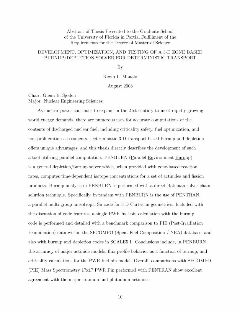
As nuclear power continues to expand in the 21st century to meet rapidly growing
world energy demands, there are numerous uses for accurate computations of the
contents of discharged nuclear fuel, including criticality safety, fuel optimization, and
non-proliferation assessments. Deterministic 3-D transport based burnup and depletion
offers unique advantages, and this thesis directly describes the development of such
a tool utilizing parallel computation. PENBURN (Parallel Environment Burnup)
is a general depletion/burnup solver which, when provided with zone-based reaction
rates, computes time-dependent isotope concentrations for a set of actinides and fission
products. Burnup analysis in PENBURN is performed with a direct Bateman-solver chain
solution technique. Specifically, in tandem with PENBURN is the use of PENTRAN,
a parallel multi-group anisotropic Sn code for 3-D Cartesian geometries. Included with
the discussion of code features, a single PWR fuel pin calculation with the burnup
code is performed and detailed with a benchmark comparison to PIE (Post-Irradiation
Examination) data within the SFCOMPO (Spent Fuel Composition / NEA) database, and
also with burnup and depletion codes in SCALE5.1. Conclusions include, in PENBURN,
the accuracy of major actinide models, flux profile behavior as a function of burnup, and
criticality calculations for the PWR fuel pin model. Overall, comparisons with SFCOMPO
(PIE) Mass Spectrometry 17x17 PWR Pin performed with PENTRAN show excellent
agreement with the major uranium and plutonium actinides.
10

CHAPTER 1INTRODUCTION
1.1 Introduction and Study Overview
Nuclear fission power reactors will likely be the most significant basis of new energy
generation in the 21st century. Fuel in fission reactors undergoes constant change as
power is generated, where fission products and actinides are continuously formed, and
these thereby transmute, often resulting in reactivity and power shifts, and changes
in fundamental cycle specific parameters. Hence, a detailed, three-dimensional (3-D)
geometric profile and specific information regarding the nature of burnup and depletion
are required to properly account for anticipated reactor physics behavior, fuel performance
and optimization, and address inventory and non-proliferation issues.
A brief discussion of theory related to the concept of depletion is provided along with
pointers to relevant literature. The overall concept of depletion or burnup, with a specific
interest in nuclear fission reactors, ties academic topics available (but not limited to)
nuclear physics, nuclear reactor engineering, transport theory, and multigroup cross section
generation. The depletion/burnup solver, PENBURN, is a computational code written
in Fortran 90/95. As of 2008, the advantages of computational modeling on serial and
parallel architectures provides accessibility to computer technology which was previously
cost-prohibitive and with resources limited to industry. This chapter also addresses
computational/programming considerations to be made in attempts to model the physics
involved.
1.2 Motivation
Currently, 3-D burnup and depletion solvers either rely on diffusion theory[1] or
recently on the introduction of Monte Carlo based burnup[2]. Monte Carlo based burnup
can be problematic when simulations call for large heterogeneous systems (multiple
fuel pins or assemblies), which in turn, motivates a study to resolve those issues within
Monte Carlo or to seek out alternatives, such as 3-D deterministic transport[3]. This
11

thesis addresses the pairing of burnup/depletion with 3-D discrete ordinates deterministic
transport.
The remaining chapters are intended to provide sufficient background and theory on
burnup, a discussion of previous work in burnup/depletion development, and a discussion
of necessary code modules and sequences (multigroup cross section processing with
the DEV-XS procedure, the algorithm development behind PENBURN, and also the
BURNDRIVER script, which runs the PENTRAN/PENBURN suite). Finally, a single
PWR pin model is modeled and compared to the SCALE5.1 burnup/depletion code
sequence and real world post-irradiation examination (PIE) data for a PWR. Lastly,
conclusions and suggestions for future work are provided.
12

CHAPTER 2THE PHYSICS OF BURNUP AND DEPLETION
The PENBURN code uses the method of modeling burnup chains solved directly
from the Bateman equations, as this method avoids the need for an ODE solver. In this
chapter, we discuss burnup of the 149Sm production chain to provide a concrete example
of the physics of burnup and depletion (Bateman Equations, fission product yields
and related data, and multigroup cross section generation). Also, a section on neutron
transport theory provides a discussion of the linear Boltzmann equation and the discrete
ordinates (SN) method.
2.1 Burnup Example
In order to track burnup and depletion, first, some explanation is warranted.
Typically, nuclide transmutation can be rather complex, as seen in Figure 2-1. A full
understanding of this figure provides the basic foundation for concepts in burnup and
depletion. First, because of the keen interest in tracking fission productpoisons, the chain
in Figure 2-1 depicts pathways to 149Sm production (note that not all possible pathways
and yields are displayed in the figure). After 135Xe, 149Sm has the highest absorption cross
section (approximately 41000 barns) and appreciable yield. Second, the downward-right
arrows with the ’y’ character indicate nuclides with production yields predominantly from
235U fission. Right arrows generally indicate (n,γ) or capture, and a down arrow indicates
a β- decay with an associated decay time. A complete understanding of this chain is
backed with foundations in the batch and production Bateman equations, explained in
the next section. For now, each nuclide can be thought of as having an individual dNdt
production and destruction rate equation, with a production term driven by neutron flux
and a loss term based on decay.
The method of solution which the burnup operates on is the linear chain method
solution of the ’direct’ Bateman Equations. I have developed an algorithm to enumerate
linear chains from an extensible complex nuclide chain model, which is provided as
13

Figure 2-1. Decay and transmutation pathways to 149Sm.
a separate input to PENBURN. Secondly, by design of the code, the mapping or
superposition of linear chains is decided by the library developer within the input library
file. This development provides a code engine, as it provides extensibility for future users
to improve physics and accuracy of the code, with the improvement and refinement of the
path matrix input.
For example, linear chains must be enumerated from the chain described in Figure
2-1, and result in six linear chains when properly calculating contributions to 150Sm,
151Sm, and 152Sm. The resulting enumeration is displayed in Figure 2-2.
More will be discussed later in how chains are mapped in the PENBURN code. For
now, we discuss related topics for background.
2.2 3-D Transport Theory and Computation
The balance of neutrons in a fission system is accomplished precisely through the
solution of the Boltzmann (”transport”) equation, which describes the behavior of neutral
particles in terms of spatial, angular, and energy domains as they interact in a system; the
time-dependent forward fixed source form of the transport equation is given in Equation
2–1 using standard notation[4].
14

Figure 2-2. Linear chain enumeration required for calculating contributions to 150Sm,
151Sm, and 152Sm.
1
v
∂ψ(~r, Ω, E)
∂t+ Ω · ∇ψ(~r, Ω, E) + σ(~r, E)ψ(~r, Ω, E) =
∞∫
0
∫
4π
dE ′dΩ′σs(~r, Ω′ · Ω, E ′ → E)Ψ(~r, Ω′, E ′) + S(~r, Ω, E)
(2–1)
The left side of Equation 2–1 represents time dependence, streaming and collision
terms (loss), respectively, and the right side represents scattering and sources (gain). Since
the transport equation describes the flow of radiation in a 3-D geometry with angular and
energy dependence at a snapshot in time, this is one of the most challenging equations
to solve in terms of complexity and model size. The source term can be an independent
surface source or independent volume source.
The discrete ordinates SN formulation evaluates a solution of angular flux in a set of
discrete directions or angles. In addition to the discrete treatment of the angular variable,
space and energy are also treated discretely. One additional complication to the solution
process is the angular quadrature selection. Angles are not arbitrarily chosen, rather, a
quadrature set consisting of weights and direction cosines is selected. A quadrature set
15

must be chosen to preserve Legendre scattering moments and be relevant to the properties
of the problem.
2.3 Radioactive Decay, Production, and the Bateman Equations
Radioactive decay processes characterize a nuclide and disintegration of its atoms to
another unique nuclide. The key measurement to be made for nearly every nuclide is the
measurement of the half-life, which is amount of time it takes for the nuclei present to
disintegrate to half of the amount present. Multiple modes of decay must be accounted
for: alpha (α), beta minus (β-), beta plus (β+), gamma (γ), isomeric transition (IT),
spontaneous fission (SF) and others. Introductions to more specialized modes of decay are
discussed and detailed within the Chart of the Nuclides[5], and other similar resources.
Solution of linear chains of radioactive or batch decay are solved by the Bateman
equations, which govern a set coupled, first order, ordinary differential equations.
Generally, the Bateman equation is labeled in a dNdt
differential rate, or in the direct
solution of the differential form, which is derived and presented in Appendix A. However,
the final derivation provides the direct solution which will be referred to as the batch
Bateman Equation. This is emphasized to distinguish the fact that the solution of the
equations is not developed from dNdt
rate for the ith nuclide, from which numerical methods
to solve coupled ordinary differential equations can be applied. The two forms of the
Bateman equations are presented in Equation 2–2 and Equation 2–3 (batch Bateman).
The batch Bateman equation assumes that no there are no sources of any of the nuclides
in the chain other than by reactions within the chain. The decay constant λi is simply the
disintegration rate per second of decay for the ith nuclide in the chain.
dNi
dt= λi−1Ni−1 − λiNi (2–2)
Ni(t) = N01 λ1λ2 . . . λi−1
i∑j=1
e−λjt
∏
k=1k 6=j
(λk − λj)(2–3)
16

Equation 2–2 and Equation 2–3 effectively describe the conditions for a linear chain
subject to initial conditions driven by only the first nuclide in the linear chain. For a
more general formulation, arbitrary initial amounts N0l are to be considered. Each finite
amount of N0l initiates a linear chain which can be added by superposition. Hence, the
batch Bateman equation can now be considered for arbitrary amounts N0l , and also for
transmutation in Equation 2–4.
Also, another distinction between Equation 2–3 and 2–4 is that there are two different
types of decay constants in use, η and µ, instead of λ. Again, the decay constant λ
by itself refers to the radioactive decay rate constant. The decay constant η is the
chain-linking precursor, which can either be a λ or σφ, where σφ is an effective reaction
rate. The reaction rate is composed of the multiplication of the reactor flux, φ, and
the microscopic cross section, σ, (typically capture). The aforementioned quantities are
integrals over all energies, but approximated as a sum over a few collapsed energy groups.
The new effective decay constant, µ, is the sum of all possible removal rate constants,
λ and σφ (if applicable to ith nuclide). Hence in the more generalized formulation
(Equation 2–4), the transmutation of a nuclide to another nuclide within the same
linear chain can be accounted for with the incorporation of both η and µ. In some
instances of the general batch Bateman equation, branch fractions for the ith nuclide must
be considered, where appropriate, and premultiplied with ηi decay constant for proper
treatment.
17

Ni(t) =i−1∑
l=1
N0l ηlηl+1 . . . ηi−1
i∑j=1
e−µjt
i∏
k=lk 6=j
(µk − µj)
+ N0i
(e−µit
µi
)
where
Ni(t) ≡ is the number of atoms for the ith nuclide at time t
N0i ≡ is the initial number of atoms for the ith nuclide at time 0
ηi ≡ is the chain-linking precursor decay constant for the ith nuclide
µi ≡ is the effective decay constant for the ith nuclide (sum of all removal rates)
(2–4)
Additionally, since reactor fluxes contribute to reaction rates, a modification to
the original batch Bateman equation is made to account for production. The Bateman
equation [6] for production is provided below in Equation 2–5, where Pl is the constant
production rate of formation of nuclide l (if nuclide l has an associated fission yield),
where, as previously defined, ηl is the chain-linking precursor rate constant, and µi is the
effective decay constant. The development of this equation assumes no initial amount
(in atoms) of nuclide Ni. Also, Qi on the left-hand side, and Pl on the right-hand side,
are distinctly two different units. Q(t)i is amount (in atoms) of nuclide i produced at
time t, and Pl is the constant rate of formation for nuclide l, in units of sec−1. Thus, the
production Bateman equation accounts for new in-growth of fission product yield rates
attributed to the parent fissile nuclide, also accounting for respective removal-rates within
the chain from nuclide in-growth.
18
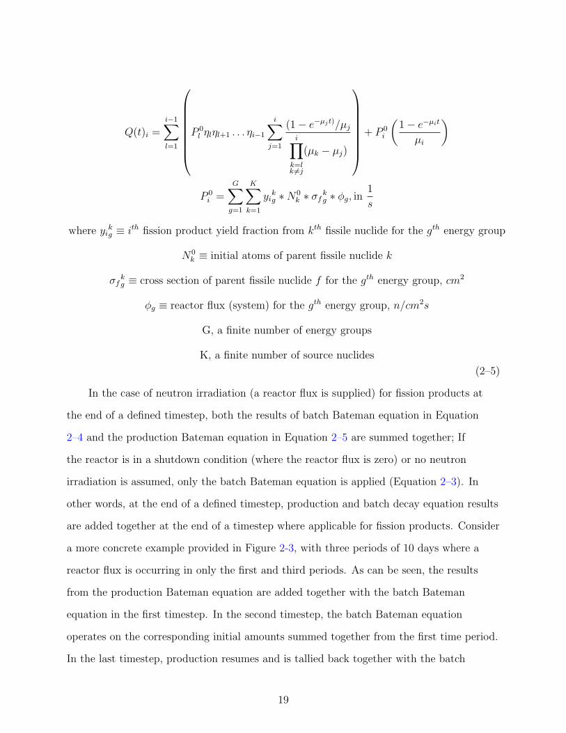
Q(t)i =i−1∑
l=1
P 0l ηlηl+1 . . . ηi−1
i∑j=1
(1− e−µjt)/µj
i∏
k=lk 6=j
(µk − µj)
+ P 0i
(1− e−µit
µi
)
P 0i =
G∑g=1
K∑
k=1
yikg ∗N0
k ∗ σfkg ∗ φg, in
1
s
where yikg ≡ ith fission product yield fraction from kth fissile nuclide for the gth energy group
N0k ≡ initial atoms of parent fissile nuclide k
σfkg ≡ cross section of parent fissile nuclide f for the gth energy group, cm2
φg ≡ reactor flux (system) for the gth energy group, n/cm2s
G, a finite number of energy groups
K, a finite number of source nuclides
(2–5)
In the case of neutron irradiation (a reactor flux is supplied) for fission products at
the end of a defined timestep, both the results of batch Bateman equation in Equation
2–4 and the production Bateman equation in Equation 2–5 are summed together; If
the reactor is in a shutdown condition (where the reactor flux is zero) or no neutron
irradiation is assumed, only the batch Bateman equation is applied (Equation 2–3). In
other words, at the end of a defined timestep, production and batch decay equation results
are added together at the end of a timestep where applicable for fission products. Consider
a more concrete example provided in Figure 2-3, with three periods of 10 days where a
reactor flux is occurring in only the first and third periods. As can be seen, the results
from the production Bateman equation are added together with the batch Bateman
equation in the first timestep. In the second timestep, the batch Bateman equation
operates on the corresponding initial amounts summed together from the first time period.
In the last timestep, production resumes and is tallied back together with the batch
19
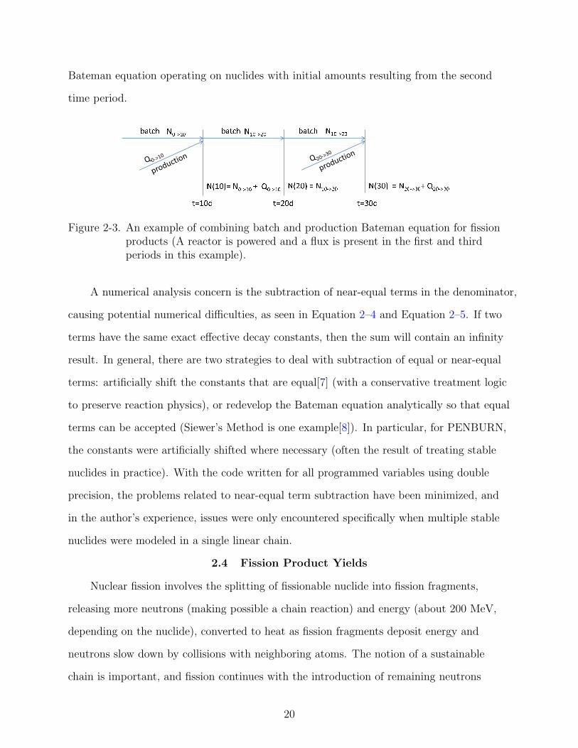
Bateman equation operating on nuclides with initial amounts resulting from the second
time period.
Figure 2-3. An example of combining batch and production Bateman equation for fission
products (A reactor is powered and a flux is present in the first and thirdperiods in this example).
A numerical analysis concern is the subtraction of near-equal terms in the denominator,
causing potential numerical difficulties, as seen in Equation 2–4 and Equation 2–5. If two
terms have the same exact effective decay constants, then the sum will contain an infinity
result. In general, there are two strategies to deal with subtraction of equal or near-equal
terms: artificially shift the constants that are equal[7] (with a conservative treatment logic
to preserve reaction physics), or redevelop the Bateman equation analytically so that equal
terms can be accepted (Siewer’s Method is one example[8]). In particular, for PENBURN,
the constants were artificially shifted where necessary (often the result of treating stable
nuclides in practice). With the code written for all programmed variables using double
precision, the problems related to near-equal term subtraction have been minimized, and
in the author’s experience, issues were only encountered specifically when multiple stable
nuclides were modeled in a single linear chain.
2.4 Fission Product Yields
Nuclear fission involves the splitting of fissionable nuclide into fission fragments,
releasing more neutrons (making possible a chain reaction) and energy (about 200 MeV,
depending on the nuclide), converted to heat as fission fragments deposit energy and
neutrons slow down by collisions with neighboring atoms. The notion of a sustainable
chain is important, and fission continues with the introduction of remaining neutrons
20

emitted into the fissile nucleus, causing new fissions to sustain the reaction. Fission,
dependent on fissile isotopes, has been demonstrated to be empirically distributed into a
double-humped fission yield curve (with statistical variation), with peaks occurring in the
neighborhood of mass numbers 90 and 140 illustrated in Figure 2-4. Clearly, fission curves
are dependent on energy and the fissile nuclide type. Common fissile parent nuclides, like
235U and 239Pu, in a critical assembly, provide percentage yields to fission products, and
empirical yield data which must be used for use in computation.
Figure 2-4. Fission yield curves (fast energy) for 238U and 232Th
Fission product yield data can functionally change, depending on neutron temperature
or neutron energy. Since fission occurs at varying energies, a common categorization
occurs in three energy intervals: thermal (upper limit (UL) of 0.0625 eV), epithermal
(UL=1 MeV), and fast (UL=20 MeV). To account for energy variation, PENBURN
computes an average energy and interpolates accordingly between the available energy
group yield values (if there is more than one energy group available).
21
Also, specific to fission product yield data is the selection of cumulative or
direct/independent yields (will henceforth refer to ’direct’ yields). Specifically, a fission
product nuclide has a cumulative yield and a direct yield value; the cumulative yield is
always greater than or equal to the direct yield. For example, consider the linear chain
(U → V → W → X →) where → designates β− decay. Suppose U and V have half-lives
(corresponding to β− decay) which are less than a minute, but W and X have half-lives
valued on the order of days. In this instance, it may not be practical to model U and V if
timesteps to be modeled are on the order of days; the cumulative yield would then be the
most appropriate selection for W since it most properly represents the aggregative yield.
The cumulative yield for W is the sum of the direct yields of U, V, and W. The nuclide X
should use the direct yield. W is then the first fission product parent in the linear chain.
By default, PENBURN applies a cumulative yield for the first fission product nuclide and
direct yields for successive fission product nuclides. However, this is not mandatory and
the library developer has the option to change between direct and cumulative yields for a
fission product.
Experimental collection of fission product yield data is not a task left to a single
individual. Data (”England and Rider” data) collected by Los Alamos National
Laboratory seems to be the most complete and openly available[9]; fission yield data
from this source is provided for 31 actinides at thermal, fast, and epithermal energies. Of
the 31 nuclides, 5 nuclides have yields for three energies, 3 nuclides have yields for two
energies, and 23 have yields for just one energy. This data has been incorporated into the
PENBURN code, discussed later.
2.5 Multigroup Cross Section Generation - Theory
Neutron cross sections are not smooth transcendental functions, and are dependent
based on material, energy, angle, and time. Readers not familiar with the variability of
neutron cross sections as a function of many variables are encouraged to refer to common
textbooks in nuclear engineering[10]. The ’continuous’ or point-wise cross sections are
22

suitable for use in continuous-energy Monte Carlo transport solvers, but are not practical
in 2-D and 3-D deterministic transport methods due to computational time constraints
and strategies used at present. Therefore, a discretization in energy must be made to be
used for modeling. Depending on the selection of the number of those energy intervals and
location of energy intervals, the continuous cross sections are ’averaged’ over a particular
interval with appropriate energy dependent flux weightings. In this case, ’averaged’
refers to the fact that we are accounting for a multitude of problems and methods of
cross section treatment beyond the scope of the discussion here: initial interpolation of
continuous cross section data, doppler broadening, resonance integral handling, unresolved
resonance self shielding, heating and radiation damage, flux weighting function selection,
spatial self-shielding corrections, multigroup structure, cross section dependencies related
to burnup, etc. Therefore, requisite knowledge of cross section development cannot be
constrained to a single paragraph, and should be investigated by the reader if not familiar
with common cross section formulations. An example of a point-wise cross section and a
multigroup cross section is provided in Figure 2-5 (visualization generated by NJOY[11]).
Although the intricacies of multigroup cross section development have many options
and are also problem specific, scientists and researchers will generally agree that cross
section measurement, verification, and validation ultimately drive the accuracy of
computational models. For this work, cross sections were developed using SCALE5.1
and/or NJOY, and are described in a separate chapter in this thesis, and include a
discussion of the ’DEV-XS’ procedure used for deterministic cross section generation at
the University of Florida.
While the task of developing multigroup cross sections appears daunting, it is within
in the realm of acceptability and pragmatism that one can generate multigroup cross
sections for use with deterministic transport. Validation of 3-D neutron transport models
and comparisons to different solution methodologies in continuous-energy Monte Carlo
(using point-wise cross sections) have been performed. An array of new research in this
23

Figure 2-5. Generation of multigroup cross section using NJOY (denoted by ”stair-step”values) for 243Pu
decade provides new insights in comparing transport solution methods (Linear Boltzmann
Multigroup Transport versus Continuous-Energy Monte Carlo), and tandem approaches
increase confidence in computational models; a strong argument can be made that Monte
Carlo and 3-D deterministic methods are needed side-by-side for large, heterogeneous
radiation transport systems[12].
24

CHAPTER 3PREVIOUS WORK
3.1 Existing Burnup/Depletion Codes
Burnup/Depletion codes have been developed, or are currently in development to
support (or eventually support) a variety of activities: tracking of major/minor actinides
in fuel, fission product generation and tracking, optimization and maximizing utilization of
nuclear fuel, validation of commitments in support of nuclear nonproliferation, open/closed
fuel cycle studies, etc.
CINDER‘90[13] adopts a linear chain method solution which PENBURN most closely
resembles in solution methodology. Also, a library with development of unique linear
chains is included, which appears to be similar in functionality to the ’path matrix’ used in
PENBURN (described later in this thesis).
The ORIGEN code provides the basis for point-depletion within SCALE5.1. It is tied
to transport solutions with NEWT, a 2-D Extended Step Characteristic (ESC) -Based
Transport Solver or KENO-VI, a Monte Carlo Solver.
Also, of recent interest in 2005, open-source software for the study of radioactive
and stable isotope transmutation chains was provided by the State Scientific Centre of
Russia - Research Institute of Atomic Reactors, in particular, a GUI-based ChainSolver
program with numeric solution under the choice of one of the following computer-aided
ODE routines: VODE,LSODA,RADAU, and MEBDF[14]. The software, as of 2008, is
currently available on the internet[15].
3.2 Monte Carlo Stochastic Methods versus Deterministic Methods for 3-DBurnup
Both the MCNP5 Monte Carlo Neutral Particle code provided by LANL (MCNP5)
and KENO within SCALE5.1 provided by ORNL are widely available to industry and
academia domestically in the U.S., and also internationally through export-licensing. The
statistical nature of these codes requires careful consideration of fission source convergence
with multiple fuel pin systems, fuels with different enrichment, assembly and full reactor
25

models, and loosely coupled systems. With this consideration, statistical tests are used to
detect for non-convergence, such as ”drift-in-mean”, ”1/N”, and Shannon Entropy (SE)
tests[3]. Exploration and remediation of fission source convergence for loosely coupled
systems is ongoing in research when Monte Carlo is used. This is not an issue for 3-D
deterministic transport, since deterministic methods yield an entire simultaneous solution
converged over a global phase space.
26

CHAPTER 4MULTIGROUP CROSS SECTION DEVELOPMENT WITH DEV-XS
DEV-XS, developed principally by the PENBURN team at the University of Florida,
is the name of a macroscopic cross-section processing sequence for use in deterministic
transport codes adapting SCALE5.1 microscopic cross sections. This chapter gives a
summary of cross section processing from both SCALE5.1 and NJOY99 output. It should
be noted, that while macroscopic cross sections are needed for transport, PENBURN uses
the microscopic cross sections collapsed to a user-specified number of broad groups from
either SCALE5.1 or NJOY.
4.1 Summary of Cross Section Processing
The development of cross sections, as previously discussed, is not trivial, so
PENBURN relies on the generation of self-shielded multigroup microscopic cross sections
by using the T-NEWT Control Sequence and ALPO, modules available within the
SCALE5.1 package. Additionally, for a minor set of fission product nuclides (<10),
multi-group self-shielded cross sections that were not available in SCALE5.1 were obtained
through NJOY‘99 and TRANSX [11]. However, SCALE5.1 provides the major share of
cross sections used in PENBURN, as it accounts for approximately 95% of the fission
products and all of the major and minor actinides.
In order to blend microscopic cross sections into material macroscopic cross section
data, one must first extract problem dependent microscopic cross sections. The SCALE
5.1 package[16] is used along with a cross section extraction card called ALPO in order
to gain access to flux weighted cross section data. Following extraction of flux weighted
microscopic cross sections through SCALE5.1, the remainder of cross section processing
is performed primarily using the Linux operating system (although the sequence can
be performed on Windows) in order to take advantage of two Linux Perl scripts,
GMIXFORM and COLLAPSEFORM. Based off of the user’s SCALE input, GMIXFORM
produces the prbname.gmx file and COLLAPSEFORM produces the prbname.grp file,
27

which are both needed by GMIX. GMIX is an important tool for group cross section
mixing and a primary component of DEV-XS, and is discussed in the next section. The
last file needed by GMIX is prbname.xsc, which is generated by post processing SCALE5.1
output products with SCALFORM. This code simply ”organizes” the cross section data
produced by the TNEWT control sequence. The structure and order of file processing will
be further described in latter sections. Figure 4-1 is a flowchart which illustrates the entire
’DEV-XS’ cross section development process. !"#$%&'()*+,(+-.*)./,0123456783 97::;<=6783>? > ?@A BCD =9;:6783EF" ?@AGHIJ# !" ?@ AK
=;8
LMNMOBCP QRST U VRWXEF@Y @Z [YG
Figure 4-1. Program structure of DEV-XS
4.2 Development of Microscopic Cross Sections Using GMIX
After each burnup/irradiation stage (typically specified on the order of hours or days),
the same microscopic cross sections are ’blended’ into new macroscopic cross sections as
the fuel is transmuting during the burnup life cycle. As briefly mentioned, cross section
mixing is achieved with an in-house code called GMIX. GMIX requires a multigroup
upper energy (MeV) bin definition file (grp file), microscopic cross sections in ANISN
format (produced by SCALFORM), and a main input deck, which defines the macroscopic
28

material, by weight fraction or atom fraction in element, and then also by weight fraction
or atom fraction defined for nuclides within each element.
4.3 The SCALE 5.1 - TNEWT Control Sequence
SCALE 5.1 is a multi-purpose, modular code that can perform criticality safety,
radiation shielding, reactor physics, spent nuclear fuel/ high-level waste (SNF/HLW)
characterization, and most importantly, cross-section processing. SCALE 5.1 contains
several control sequences which perform a series of linked calculations with executable
modules. TNEWT is the control sequence which will perform resonance reconstruction,
temperature-dependent Doppler broadening for resonances, process S(α,β) data for
thermal moderators, and flux-weighted group collapsing.
When the TNEWT control sequence is performed, there are five modules called in
SCALE5.1:
1. BONAMI- unresolved resonance self-shielding processor using the Bondarenko
Method.
2. CENTRUM- creates space dependent (1-D), point wise continuous-energy, flux file.
3. PMC- creates a problem-dependent master library from the CENTRM flux
spectrum.
4. WORKER- creates Working libraries from Master libraries.
5. NEWT- 2-D discrete ordinates transport solver which performs cross-section group
collapsing.
A SCALE Module named ALPO is used to dump the collapsed cross section data
from the TNEWT scratch file to a temporary file, which can be redirected by the user.
4.4 Reformatting Of SCALE5.1 Output Data UsingSCALFORM,GMIXFORM, and COLLAPSEFORM
A series of codes and scripts were developed to automatically generate necessary
inputs for both PENTRAN and PENBURN. Each of the codes or scripts is developed
to generate specific input. The three codes/scripts in this section end with the suffix
29

”-FORM” to indicate form generation from SCALE5.1 output. The inputs generated feed
into GMIX
The cross section data obtained from using the ALPO cross section extraction card
is filtered and reorganized to the standard format (accepted for use in PENTRAN) using
SCALFORM, a Fortran 90/95 code. When SCALFORM is called, the user inputs the
name of the cross-section file, the number of energy groups, and relevant cross section
table parameters.
The Perl scripts (Linux OS), GMIXFORM and COLLAPSEFORM, automate the
creation of these files needed for GMIX, a main input file (prbname.gmx) and an energy
multigroup file which simply lists the upper energy bounds of each group in MeV units.
The only file needed by these scripts is the SCALE5.1 input.
4.5 A Multigroup Cross Section Generator and Library Formatter UsingNJOY99 and TRANSX
The SCALE5.1 code package is capable of producing a majority of the cross sections
necessary for the PENTRAN/PENBURN suite, however there are around 20 nuclides
that are unobtainable due to a lack of data within the SCALE 238 group AMPX library.
To account for these gaps in cross section data, the NJOY processing system has been
incorporated into the DEV-XS procedure.
NJOY99.0 is a comprehensive computer code package that produces multigroup
transport cross sections from evaluated nuclear data which is in the ENDF format. NJOY
consists of a set of at least 24 modules, each designed to perform a specific task. The
following seven NJOY modules are used to generate the missing SCALE cross section data
for the PENTRAN/PENBURN suite:
RECONR Reads an ENDF tape and produces a common energy grid for all reactions
such that all cross sections can be obtained to within a specified tolerance by
linear interpolation. Creates point-wise cross sections which are written onto a
”point-ENDF” (PENDF) tape for future use.
30
BROADR Reads a PENDF tape and Doppler-broadens the data using the accurate
point-kernel method. After broadening and thinning, the summation cross sections
(total, inelastic) are written to a new PENDF tape for future use.
UNRESR Produces effective self-shielded pointwise cross sections, versus energy and
background cross-section in the unresolved range. This is done for each temperature
produced by BROADR, using average resonance parameters from the ENDF
evaluation. Results are once again added to the PENDF tape.
THERMR Produces pointwise cross sections in the thermal range. Energy to energy
incoherent inelastic scattering matrices can be computed for free-gas scattering or for
bound scattering using a pre-computed scattering law S(α,β) in ENDF format.
GROUPR Processes the pointwise cross sections modified by the modules described
above into multigroup form, based on a specific group structure and weighting
function. NJOY has the option of using a built-in or custom weighting function for
cross section group collapsing. The resulting file is referred to as a GENDF tape.
PLOTR/VIEWR Creates a postscript file for a visual validation that a proper group
collapse has been performed relative to the pointwise data.
MATXSR Formats multi-group data from GENDF file and converts GENDF to MATXS
format, which is suitable for separate code called TRANSX, which is capable of
producing the desired ANISN library format for PENTRAN/PENBURN.
4.6 Burnup Dependent Cross Sections
One must typically account for burnup influence on microscopic cross sections;
however, previous references cite that reprocessing microscopic cross sections after each
burnup stage is not necessary for low burnups [17] or for nuclide number densities below
10-3 atoms/bn-cm [18]. Therefore, we limited our study to problems which do not extend
beyond 20 GWd/MTHM. Additionally, the same initial microscopic cross sections are used
from the zeroth timestep, where macroscopic cross sections are redeveloped for transport.
Also, it should be noted that multigroup collapse to three energy groups is performed with
31

the T-NEWT Control Sequence from SCALE5.1, using the general 238-group library in
SCALE5.1.
This chapter summarized key code components of the DEV-XS procedure for
preparation of macroscopic cross sections for transport. In the next chapter, a discussion
of PENBURN development is presented.
32

CHAPTER 5PENBURN CODE DEVELOPMENT AND FEATURES
The use of the linear chain method is not unique, as it has been used in codes such
as CINDER‘90 [13], as mentioned previously. A unique asset of the PENBURN code is
that it was designed to incorporate a numeric path scheme called the ’path matrix’ which
effectively describes nuclide branch pathways linked by neutron capture, β- decay, α decay,
or isomeric transition (IT) by metastable nuclides to ground-states. The path matrix
describes all branch decay-transmutation chains. A thorough and recommended discussion
of linear chain modeling is available in prominent texts [6].
The next section discusses an implementation of linear chain modeling performed by
developing a path matrix input file. It should be noted that most end-users or evaluators
of the code will not actually spend time developing this file, as one has already been built
by the author. The ability to extend (or scale back) modeling for new nuclides not covered
by the current library may be of direct interest to users of the code, or for those that want
to understand how the modeling within PENBURN works.
5.1 Linear Chain Modeling
The core algorithm development in PENBURN develops enumerated linear chains
from a path matrix input. To clarify, unique linear chains are not provided in a library;
PENBURN interprets a complicated chain and enumerates all of the possibilities available.
We shall present the idea drawn from a conceptual example in Figure 5-1.
To avoid confusion, it should be mentioned that the numbers identified in the
drawings in Figure 5-1 and Figure 5-3 are merely IDs for the nuclides where normally
letters should be used. In this case numbers were used because of their suitability for
programming in Fortran90/95.
A concept of how a complex chain is loaded is shown in an embedded table with a
drawing of the chain in Figure 5-3. In the real path matrix used by PENBURN, column
1 is omitted and is ’implicit’, but is indicated in the figure to denote the importance of
33

implicit row indexing for use in the path matrix; the implicit row indicates the ’pointees’
that the links point to. Also, implicit rows serve as aliases for the true nuclide ID. For
example, nuclide ’2’ has two links to implicit rows ’3’ and ’5’ which correspond to nuclide
ID’s ’3’ and ’6’ respectively.
The link column establishes the number of links (or connecting arrows) for which the
nuclide serves as the precursor; Figure 5-3 makes it apparent that only nuclide ’2’ has two
links. The remainding columns, which by default are set to zero, are filled with pointers to
the implicit row values or the ’pointees’. In PENBURN, in place of the second column, the
identification column, is the real ZAID assignment. For example, 92235 would be listed
in the identification column, however, it would have an implicit ID of ’1’, since pointer
assignments are more convenient with a natural number ordering system (1,2,3,. . . ) than
with a ZAID system. The complex chain, if possible, should end at a stable nuclide. That
is why nuclide ’4’ is designated on implicit row six, the last row for the chain. The implicit
ID, along with a ZAID alias, simply operates just as described in Figure 5-3. A more
thorough discussion of the ZAIDs is presented in Section 5.1.3.
Since PENBURN can enumerate the linear chains, the concept of superposition is
used to directly solve a production Bateman equation (assuming irradiation), and a batch
Bateman equation, for the ith nuclide in the linear chain. However, superposition only
applies when adding ”unique” linear chains. Again, by code design, it is left to the library
developer to assign values to a map matrix so that only the unique linear chains are added
back together.
At the current stage of development within PENBURN, the resulting enumeration
from a complex chain results in Figure 5-2. A scheme for defining only the summation
of unique linear chains is performed by taking the resulting enumerated chains and
employing one-for-one replacements, such that the library developer generates a modified
enumerated chain called the ’map matrix’ developed in Figure 5-3. It seems feasible
enough, that in future development, an algorithm can be developed to perform the
34

Figure 5-1. Example of developing linear chains from a more complex chain
necessary modifications to generate the map matrix, which, again, is viewed in Figure 5-3.
For clarity, it should be taken that the words ’entry’ and ’value’ are interchangeable.
In Figure 5-3, each row represents an enumerated linear chain (with one-for-one
replacements from Figure 5-2) with positive nuclide ID values, a ’0’ value, negative nuclide
ID values, or a ’-99’ value. A ’0’ value prevents the summation of a repeat instance of
a nuclide. In the example in chain 2, ’1’ and ’2’ are replaced with ’0’ and ’0’, so as to
prevent the unnecessary doubling of contributions to nuclides 1 and 2. A negative nuclide
ID value assignment prevents a particular chain sequence from contributing; this is best
illustrated with the example. In chain 2 of Figure 5-3, ’3’ and ’4’ are replaced with ’-3’
and ’-4’. The unique sequences ’1 → 2 → 6 → 3 → 4 →’, ’2 → 6 → 3 → 4 →’, and
’6 → 3 → 4 →’ are unique whereas ’3 → 4 →’ and ’4 →’ are not (repeated from chain
1), so negative nuclide ID assignment suppresses them. Finally, a ’-99’ value combines
35
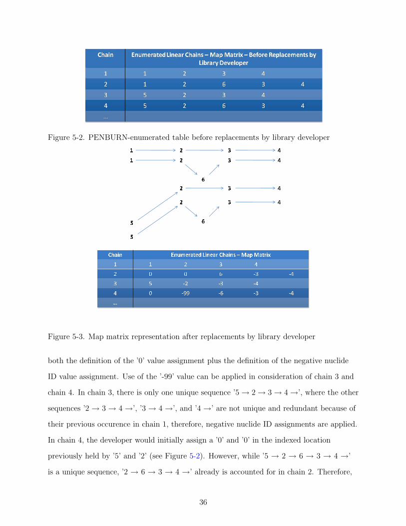
Figure 5-2. PENBURN-enumerated table before replacements by library developer ! " " # " " " "$$ "! " "%
Figure 5-3. Map matrix representation after replacements by library developer
both the definition of the ’0’ value assignment plus the definition of the negative nuclide
ID value assignment. Use of the ’-99’ value can be applied in consideration of chain 3 and
chain 4. In chain 3, there is only one unique sequence ’5 → 2 → 3 → 4 →’, where the other
sequences ’2 → 3 → 4 →’, ’3 → 4 →’, and ’4 →’ are not unique and redundant because of
their previous occurence in chain 1, therefore, negative nuclide ID assignments are applied.
In chain 4, the developer would initially assign a ’0’ and ’0’ in the indexed location
previously held by ’5’ and ’2’ (see Figure 5-2). However, while ’5 → 2 → 6 → 3 → 4 →’
is a unique sequence, ’2 → 6 → 3 → 4 →’ already is accounted for in chain 2. Therefore,
36

an assignment of ’0’ and ’0’ does not account for the necessity of suppressing the sequence
of ’2 → 6 → 3 → 4 →’; thus, a ’-99’ is used, which prevents the redundancy of adding
another ’2’ nuclide to itself and also preventing the ’2 → 6 → 3 → 4 →’ sequence to be
redundantly added.
There are some general principles that can be considered when constructing the map
matrix. When considering the ith nuclide, a positive nuclide ID entry should only occur
once, with successive negative nuclide ID entries. For example, nuclide ’4’ is positive once
in chain 1 and then assigned to be ’-4’ in chains 2, 3, and 4. Additionally, the ’0’ entries
should generally be employed where a repeating sequence is obvious. Also, in general, a
chain can logically begin with a series of ’0’ entries, followed by ’-99’ entries, and then
followed by negative nuclide ID or positive nuclide ID entries.
At this point, it should be said that the path matrix and map matrix are both
user-generated. But, once generated, they provide a basis library which can be continually
rebuilt or extended with the expectation that users need not enumerate the unique linear
chains. Also, the code promotes extensible design outside of the source code. Overall,
the code engine provides support for a dynamic handling of branch decay-transmutation
chains. Also, this structure enables improved physics refinements, as the code handles
nuclide chains with major modes of radioactive decay and neutron capture.
A point not yet discussed is the fact that feedback loops can be designed. For
example, along a linear chain 240Pu is an indirect precursor to 244Cm; 244Cm alpha decays
to 240Pu, seen in Figure 5-7. In particular, a duplicate nuclide 240Pu is modeled in the
linear chain to capture the resulting contribution from 244Cm α decay. At the end of a
defined timestep, the results held by the duplicate nuclide are added back to the original
240Pu nuclide. Initial analysis presumes that this method of incorporating feedback is
more accurate with smaller timesteps. For a more complex model of actinide decay and
transmutation pathways (note that α- decays are not shown), see Figure 5-8.
37

One matrix in the ’path’ input that is also necessary is called the link precursor
matrix, which basically describes what happens when a nuclide is pointing to another
nuclide by a connecting arrow. This matrix is built by the user along with the path matrix
and map matrix for the ’path’ file. An example is given in Figure 5-4. The goal of the
link precusor matrix is to properly define capture precursors within a linear chain. For
each row, there are at least three entries. The first entry is the global nuclide ID, and
the second entry indicates the number of branches. If the number of branches is one,
only one more entry is required, which points to the implicit ID which defines the linking
capture precursor. Any values larger than the number of nuclides modeled (such as ’199’,
arbitrarily chosen) indicate to PENBURN that radioactive decay is the default selection.
That is, if PENBURN cannot properly find the linking capture precursor, it assumes that
the precursor must be a form of radioactive decay for which radioactive decay constant
or half-life values are supplied (stored in PENBURN). It should be noted that with more
branches, branch fractions are required to precede the connecting implicit ID entries. In
the example of Figure 5-4, the ’-2’ on the last row refers to two branches but the negative
value indicates two β precursor links, one to an implicit nuclide ID 19 with fraction 0.654
and one to an implicit nuclide ID 20 with fraction 0.346 (the fractions summing up to
1.000).
5.1.1 Actinide Models
The actinides provided in Figure 5-6 and Figure 5-7 are modeled with the path matrix
in PENBURN, along with the additions of 243Am, 244Am, and 244Cm.
5.1.2 Fission Product Models
A host of fission products are introduced with the transmutation of actinide fuel. At
present, a minimum of 122 fission products nuclides are modeled (see Table 5-1. When a
fission product is relatively isolated and does not serve as a precursor to other nuclides (or
the fission product nuclide produced is stable) it can be labeled as a stand-alone nuclide.
In fact, all of the stand-alone nuclides are artificially inserted into one long linear chain
38

Figure 5-4. Link matrix example
with zero precursor assignment, so that for each nuclide in the chain, only production yield
rate from fissile parents and radioactive decay for the same nuclide produced is performed.
5.1.3 Metastable Nuclide Treatment and Duplicate Assignment
Also, often bypassed by other burnup codes is the modeling of metastable nuclides,
which are discriminately and effectively handled by PENBURN. ZAID values are typically
five-digit values and with Z values less than 90; thus six-digit values greater than 100000
and less than 900000 are labeled as metastable nuclides. Beyond providing for metastable
nuclide distinctions, metastable nuclides generally operate in a linear chain just like
regular nuclides. For example, 148Pm is identified as ’61148’, whereas 148mPm is labeled as
’611481’. Suppose (hypothetically) that 148Pm has a second metastable value.
There are instances where it is necessary to have a duplicate ID assignment (for
feedback loops). Specifically, suppose another 148Pm is needed, then a first duplicate
assignment would start with ’611489’, a second duplicate assignment would be ’611488’,
and so on counting backwards. Obviously, it is expected that the number of duplicates and
the number of metastable ground states is less than or equal to 10.
When identical nuclides require different microscopic cross sections, multiple indexing
(MI) is used. The multiple indexing is an optional second field, which can be valued from
39

Table 5-1. Fission product data
Fission product nuclide list.16O 77As 77Se 78Se 80Se 82Se81Br 82Br 82Kr 83Kr 84Kr 85Kr85Rb 87Rb 88Sr 89Sr 90Sr 89Y90Y 91Y 90Zr 91Zr 93Zr 94Zr95Zr 93Nb 95Nb 95Mo 96Mo 97Mo98Mo 99Mo 100Mo 99Tc 99Ru 100Ru101Ru 102Ru 103Ru 104Ru 106Ru 103Rh104Pd 105Pd 106Pd 107Pd 110Pd 107Ag111Ag 111Cd 112Cd 113Cd 114Cd 116Cd115Sn 116Sn 118Sn 119Sn 120Sn 122Sn123Sn 124Sn 125Sn 126Sn 127mTe 128Te
129mTe 130Te 127I 129I 131I 133I135I 131Xe 132Xe 133Xe 134Xe 135Xe
136Xe 133Cs 134Cs 135Cs 137Cs 135Ba136Ba 137Ba 138Ba 140Ba 139La 140La140Ce 141Ce 142Ce 143Ce 144Ce 141Pr143Pr 143Nd 144Nd 145Nd 146Nd 147Nd148Nd 150Nd 147Pm 148Pm 148mPm 149Pm150Pm 147Sm 148Sm 149Sm 150Sm 151Sm152Sm 153Sm 154Sm 151Eu 152Eu 153Eu154Eu 155Eu 156Eu 156Gd 157Gd 158Gd159Gd 160Gd
0 to 999. For example, microscopic cross sections can also be spatially dependent, and
consequently, there are instances when differently valued microscopic cross sections are
needed for the same nuclide. In this case, a multiple index option is used. Consider an
example where ground state 242Am required 2 spatially dependent zones, the identifier
assignment should be ’95241 1’ and ’95241 2’. If metastable 242mAm required 2 spatially
dependent zones, the identifier assignment should be ’952411 1’ and ’952411 2’.
5.2 Reaction Rate Collection from Transport Solution
Once transport calculation of angular and scalar fluxes is completed with PENTRAN,
the scalar flux, in particular, must be multiplied with the microscopic cross section (cm2)
so that reaction rates can be calculated to contribute to the effective µ term. The effective
µ term is the sum of both σφ and λ , the decay constant (sec-1). In fact, in order not
40

to obscure the depletion module, a small code was developed in Fortran90/95 called
PENPOW (Parallel Environment Power).
A direct relationship between flux and power is used; flux can be scaled to power or
vice versa. It is noted that for any type of reactor, either the total system power or power
density, in W/(g-HM) (heavy metal) must be known. This parameter is saved for the
depletion code PENBURN, so scaling to 1 Watt of total system power is assumed.
5.3 An Introduction to PENBURN and Code Extensibility
PENBURN, of course, uses a direct Bateman solution method with the linear chains
discussed earlier this chapter. The linear chain method using Bateman equations is
actively employed by the code, all written in Fortran 90/95.
The reason for employing three groups is briefly mentioned; fission yield data sets
used by the burnup code are provided in three energy groups [9]. Therefore, appropriate
treatments for different reactor types, for example, fast reactors, will have higher accuracy
than in code systems where the available epithermal and fast fission yield data have been
ignored.
Up to this point, the actual inputs to PENBURN have not been discussed, since the
files needed are generated by other codes. Details on specific input and output by the
software programs PENPOW and PENBURN are detailed in the Appendix.
5.4 Formatted Output
A number of formatted outputs are available for the nuclides modeled. Output is
available in units of atoms/bn-cm, grams, atom percent by element, and weight percent
of total element. In fact, the requirement of each type of output is based on specific need.
Number density output in atoms/bn-cm is useful when making comparisons to other
burnup codes. Gram output is useful for comparison with real data, since measurements
are made by weight or provided as a weight ratio between two nuclides.
41

As an example, output provided by PENBURN is given in units of atom percent of
nuclide by element, which is a useful output option for examining uranium and plutonium
isotopics, seen in Figure 5-5.
Figure 5-5. Sample PENBURN output of atom percent of nuclide by element for uraniumand plutonium elements.
Figure 5-6. Actinide linear chain of 235U
5.5 Validation of the PENBURN Bateman Algorithm with MathematicaSolver
The Bateman equation subroutines in the PENBURN depletion solver were validated
for an irradiation case of 10 periods of 100 days for a total of 1000 days of irradiation
(with an assumed constant reactor flux). A Mathematica notebook with independent
solutions of the differential equations for burnup was also solved and compared to
42

Figure 5-7. Actinide linear chain of 238U
Figure 5-8. Decay and transmutation pathways for a complex actinide chain
43

PENBURN, initialized using the same η and µ decay constant values. Overall, the
difference between these two independent methods was no greater than approximately 0.01
percent at the 100 day timestep and for subsequent timesteps after, the differences were
attributed to numerical precision and exactness of supplying decay constants and atom
amounts. The companion Mathematica sheet is provided in the Appendix.
44

CHAPTER 6BURNUP DRIVER
6.1 Driver Cycle and PENBURN Integration
The merging of code sequences is achieved with the development of BURNDRIVER,
a Linux/Bash Shell driver script which runs the codes. Initially, the following tasks must
have been performed before running BURNDRIVER:
• Run SCALE5.1 ALPO to obtain microscopic cross sections
• (Optional) Run GMIX to blend microscopic cross sections into macroscopic crosssections
• (Optional) Run PENTRAN to ensure flux and criticality eigenvalue convergence
The BURNDRIVER script sequences the cycle listed in the order below (REPRO step
is optional):
1. GMIX - SCALE5.1 Microscopic XS =⇒ Macroscopic XS
2. PENTRAN - 3-D transport solver is performed
3. PENPOW - convert flux to reaction rates
4. PENBURN - burnup/depletion run
5. GMIX - new fuel composition, to obtain updated macroscopic cross sections
6. Repeat Step 2; otherwise stop after Step 2
An overview of BURNDRIVER is provided in Figure 6-1.
6.2 PENTRAN - Parallel Sn Neutron Particle Transport Code
The use of PENBURN is not purely stand-alone, since typically reactor fluxes
contribute to the calculation of reaction rates for use in any burnup code. For
computation of 3-D fluxes, the PENTRAN (Parallel Environment Neutral-particle
TRANsport) code is used [19].
The PENTRAN code system can be used for 3 D multigroup forward and adjoint
discrete ordinates (Sn) simulations. PENTRAN is actually a suite of codes that allow one
to readily generate mesh geometries and solve 3-D transport models and automatically
45

Figure 6-1. Illustration of BURNDRIVER sequence
collate parallel data. PENTRAN is a multi-group, anisotropic Sn code for 3-D Cartesian
geometries; it has been specifically designed for distributed memory, scalable parallel
computer architectures using the MPI (Message Passing Interface) library. Automatic
domain decomposition among the angular, energy, and spatial variables with an
adaptive differencing algorithm and other numerical enhancements make PENTRAN
an extremely robust solver with a 0.975 parallel code fraction (based on Amdahl’s
law). Numerous simulations have been performed using the PENTRAN code system,
including many international benchmark computations. The many advanced numerical
features in PENTRAN, including adaptive differencing with a two-level parallel angular
memory structure in a scalable architecture enable it to be used to render a solution
to extremely large-scale transport detection problems in a rapid time using parallel
computing. PENTRAN has demonstrated excellent agreement with both Monte Carlo and
46
experimental flux measurements in a variety of problems in reactor physics, detection, and
medical physics applications [19].
6.3 PENPOW - Reaction Rates and Parallel Implementation
The burnup code operates on reaction rates for a nuclide by energy group.
Multigroup fluxes are collapsed into three-group reaction rates (fast, epithermal, and
thermal) along with a total reaction rate for individual isotopes. This calculation is
primarily performed by a linker code called PENPOW, which obtains flux results scaled
from PENTRAN Sn transport and produces a file of reaction rates suitable for use in
PENBURN.
47

CHAPTER 7REACTOR PIN MODELING
In this chapter, the PENTRAN/PENBURN suite (enabled for practical use
with the BURNDRIVER) is examined and compared to SCALE5.1 and to data in a
Post-Irradiaiton Examination (PIE) database. In particular, general flux behavior as a
function of burnup, criticality, and comparisons with major actinides are performed.
7.1 Candidate Pin, Parameters, and Assumptions
SFCOMPO [20] provides PIE Data, and specifically data for 7 PWRs and 7 BWRs
from Germany, Italy, Japan, and the United States. Also, the data is comprehensive,
providing the following: reactor name and type, active height, assembly name and
location, fuel rod position, sampling position of fuel rod, initial enrichment, cooling time,
laboratory performing analysis, burnup in units of GWd/MTU, and PIE data usually in
units of kg/MTHM or by weight ratio. The initial benchmark model for PENBURN is
a 17x17 PWR, and the only reactor in the database which has the same assembly and
reactor type is the Takahama-3 reactor in Japan. One notable omission is the power
history information; only integrated burnup values are provided.
Table 7-1. Sample SF95-1 PWR UO2 pin data
Description Value UnitBurnup 14.3 GWd/MTHM
Enrichment 4.11 wt%Fuel Pitch 1.265 cm
Fuel Pitch (Effective) 1.32354 cmFuel Diameter 0.805 cmClad Thickness 0.064 cm
Fuel Temp. (Assumed) 1000 KClad Temp. (Assumed) 700 K
Moderator Temp. (Assumed) 575 K
In the Takahama-3 Reactor, 16 samples were adopted from the database and
examined. The 16 samples are taken from three separate fuel pins. Eleven samples
were UO2 fuel and 5 were UO2-Gd2O3 fuel. Of the 11 UO2, one sample was selected as
48

the benchmark candidate, specifically, fuel sample SF95-1. Table 7-1 provides relevant
parameters used in the PENBURN code study (with assumed values as indicated).
Again, one significant limitation of the SFCOMPO data for the Takahama-3 reactor
is that no power history is provided for any samples. Previous calls for benchmark studies
have indicated, for a similar sample in the same reactor (SF97-4) with a burnup of 47.03
GWd/MTHM, an assumed power history of 3 irradiation cycles of approximately 400 days
each, with approximately 80 days of downtime status in between cycles [21].
It is assumed that SF95-1 was measured after one irradiation cycle. Various estimates
in the range of 25 - 45 MW/MTHM for the power density (assumed constant through
range of cycle) were assumed and calculated. In particular, we examine the case of a lower
assumption of 25 MW/MTHM, which is assumed to be a constant power density for one
complete irradiation period. This is done, as opposed to assuming one irradiation period
followed by a period of downtime/cooling. According to NEA, a constant power density
assumption can introduce uncertainty; this can and will bias outcomes for isotopes 135Xe,
149Sm, and also isotopes depending on final burnup value, for example, various Pu isotopes
at the end of the chain depletion [21].
7.2 Candidate Pin Design
For a PWR unit cell, the detailed geometry is given for a 2-D slice of a 3-D transport
calculation in PENTRAN. To clarify, identical UO2 fuel was split into three equally,
radially segmented concentric zones. Each zone is identically the same fuel before burnup.
The three zones are labeled as 1, 2, and 3 and respectively, will be denoted as the inner
3rd, the middle 3rd, and the outer 3rd (See Figure 7-1). Another model with just a single
zone of PWR fuel was also incorporated for comparison with the 3-zone model.
For transport in PENTRAN, an S8P1 quadrature and reflective boundary conditions
were assigned for an infinite lattice calculation. A three group structure was used with
upper energy bounds at 20 MeV, 1 MeV, and 0.625 eV (respectively fast, epithermal,
and thermal energy groups). This group structure matches that by the structure used in
49

Figure 7-1. Two dimensional PWR pin geometry
the ORIGEN-S depletion module. Also, the unit cell adopts the values and parameters
provided in Table 7-1.
The PENTRAN model used a 44x44 mesh structure to optimize fuel mass balance
and yield fine detail for the three burnup zones. Flux and keff convergence requirements
were set to 1E-3 and 1E-5 respectively. For differencing methods, an adaptive differencing
method was selected.
7.3 Results and Comparison to Mass Spectrometry Data and SCALE5.1
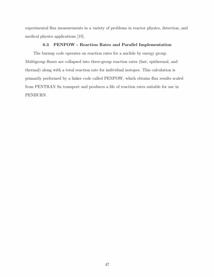
Qualitative flux plots for three groups are shown for two snapshots in time, one at
BOL and one at the desired 14.3 GWd/MTHM burnup for the SF95-1 PIE sample. For
Figure 7-3, Figure 7-4, and Figure 7-5, each group is shown side-by-side, with the fresh
fuel transport results on the left hand side, and burned fuel at discharge on the right.
Note that the white cells define the clad boundary of the fuel.
Clearly, the bulk of the fission reactions occur in the fast group, and also within the
epithermal group. Tables 7-3 and 7-4 indicate the ratio of group flux to total flux; because
the epithermal window ranges from 0.625 eV up to 1 MeV, a bulk of fissions occurring in
the keV range dominate. The same aforementioned tables also compare the 1-zone model
to the 3-zone model. The 1-zone model clearly lies in an average of the 3-zone model,
50

weighted towards the outer 3rd zone, since the outermost fuel ring contains the largest
volume of the three fuel segments. With only three radial zones, the highest fast fuel flux
value is in the inner zone and the highest thermal flux value in the fuel is on the fuel pin
rim. The same expected profile holds for the 0 and 14.3 GWd/MTHM burnups, but the
14.3 GWd/MTHM case has a higher fast to total flux ratio because of increasing fissions
coming from 239Pu.
7.4 Discussion
A TRITON model calculation from the SCALE5.1 package uses similar parameters
used in the PENBURN single zone model, as previously discussed in Section 7.1, with
the same extended burnup. To compare, the same specified burnup was considered
(14.3 GWd/MTHM).
In TRITON, the burnup and transport use a predictor-corrector approach where
transport is performed at the midpoint of each stage of burnup, and subsequently
burnup is redone back at the half-step point with cross section processing[22]. Also, the
extended step characteristic (ESC) method is used in the NEWT transport solver, which
is fundamentally different from the adaptive difference integro-differential source iteration
Sn solver used in PENTRAN. The SCALE5.1 burnup is performed by ORIGEN-S (point
depletion and decay) and employs a matrix exponential method. Because TRITON
employs a fundamentally different approach, the transport is not built for a one-to-one
comparison. As an example, Figure 7-2 indicate keff as a function of burnup. As seen
on Figure 7-2, keff values are consistently offset in PENTRAN/PENBURN compared
to the NEWT/TRITON sequence. The keff values for the 3-Zone and 1-Zone models in
PENTRAN/PENBURN nearly overlap as a function of burnup. Analysis suggests the
difference in keff noted is related to the transport differencing schemes between the two
codes. This is reasonable, since from the starting criticality configuration, the values
consistently differ by about 0.04 ∆kk
. It appears that the slopes of keff nearly drop off with
the same slope.
51

Figure 7-2. Calculation of keff values as a function of burnup to 14.3 GWd/MTHM
The Computed/Experimental (C/E) ratios are graphed in Figure 7-6 and can be also
be determined from the percent differences in Table 7-2. The maximum error of uranium
nuclides in PENBURN is 4.4 based on SFCOMPO sample data. In the plutonium series, it
should be noted that 238Pu is not modeled in PENBURN, but was reported in SCALE5.1
data. A point can be made in the accuracy of 239Pu, however, being limited to 0.4% error
in the average case, and also to just 1.1% error in the ratio of 239Pu to 238U.
Flux plots for the three groups at 0 GWd/MTHM and 14.3 GWd/MTHM are plotted
in Figures 7-3, 7-4, and 7-5. As a function of burnup, a development of fuel self-shielding
can be seen in the fast group, but at this point in burnup the shift is subtle. Tables 7-3
and 7-4 of group flux to total flux make it more apparent that the proportion of thermal
52

flux to total flux is decreasing and is compensated by a higher overall proportion of fast
flux to total flux after 14.3 GWd/MTHM. With regards to each flux plot, in the legend,
a rainbow spectrum is applied, where the high value is red and the low value is blue. The
flux plots in general (Figures 7-3, 7-4, and 7-5), also follow the trends marked by Tables
7-3 and 7-4. In Figure 7-3 for fast energies, the flux increases and also corresponds to the
increasing proportion of fast flux to total flux from 0 to 14.3 GWd/MTHM. In Figure
7-4 for epithermal energies, the flux increases. In Figure 7-5 for thermal energies, the flux
decreases, which also corresponds to the drop in proportion of thermal flux to total flux
from 0 to 14.3 GWd/MTHM.
Minor issues and accuracy for some of the plutonium nuclides may be related to
microscopic cross section change during burnup; in this comparison study, it was assumed
that cross sections do not change significantly for low burnups. However, performance
overall in PENBURN is excellent as it compares to uranium and plutonium actinides.
53

Figure 7-3. Group 1 relative flux. A) 0 GWd/MTHM. B) 14 GWd/MTHM.
Figure 7-4. Group 2 relative flux. A) 0 GWd/MTHM. B) 14 GWd/MTHM.
54
Figure 7-5. Group 3 relative flux. A) 0 GWd/MTHM. B) 14 GWd/MTHM.
55

Table 7-2. Percent differences (actinides) for PENBURN comparison to SFCOMPO (mass spectrometry based) gram ratios insample SF95-1 at 14.3 GWd/MTHM burnup
Description PB-Inner PB-Middle PB-Outer PB-1-Zone PB-1-Zone-Cm244 SCALE5.1
235U
U2.6 2.0 0.7 1.4 2.3 1.1
236U
U2.7 3.5 5.4 4.4 2.7 7.6
238U
U-0.02 ˜0 0.03 0.02 -0.01 -0.03
238Pu
Pu- - - - - -5.5
239Pu
Pu1.4 1.7 -0.1 0.4 1.0 1.5
240Pu
Pu-14 -17 -9 -11 -11.7 -6.4
241Pu
Pu19 22 25 23 19.0 -1.1
242Pu
Pu-0.8 3.5 11.1 7.0 0.8 -11.6
239Pu238U
2.2 1.7 0.6 1.1 -0.05 13.9
56

Table 7-3. Group flux to total flux ratio at 0 GWd/MTHM
Description PENBURN-Inner PENBURN-Middle PENBURN-Outer PENBURN-1-ZoneFastTotal
0.240 0.238 0.234 0.235Epithermal
Total0.641 0.641 0.640 0.641
ThermalTotal
0.119 0.121 0.126 0.124
Table 7-4. Group flux to total flux ratio at 14 GWd/MTHM
Description PENBURN-Inner PENBURN-Middle PENBURN-Outer PENBURN-1-ZoneFastTotal
0.253 0.251 0.246 0.248Epithermal
Total0.646 0.646 0.645 0.646
ThermalTotal
0.101 0.103 0.108 0.106
57

Figure 7-6. Ratios (C/E) by model
58
7.5 Results and Comparison of Selected Fission Product Data to SCALE5.1
Briefly, for the same PWR pin model burnup to 14.3 GWd/MTHM, three fission
products were selected and compared to SCALE5.1: 137Cs, 90Sr, and 95Mo. In Table 7-5,
each fission product nuclide has two rows, one with three group fission product yields
(fast, epithermal, and thermal) applied within PENBURN and another with only thermal
fission product yields applied. The aforementioned problem was investigated in order to
determine whether or not a measurable difference occurs in applying only thermal fission
product yields as opposed to the application of three group fission product yields.
Overall, as illustrated in Table 7-5, the maximum percent difference in all cases is
kept below 10.16 percent in comparing PENBURN cases to SCALE5.1 for these nuclides.
Also, in comparing the use of fission product yields for each nuclide, the change in percent
difference changes minimally, with the largest difference observed for 137Cs among those
considered here. Note that the first two comparisons for each nuclide assess the percent
difference change from SCALE5.1; the last comparison for each fission product measures
the percent difference concentration change in units of atom/bn-cm from using variable
3-group yields to using only thermal yields. Application of only thermal yields drifts the
PENBURN comparisons away from SCALE by approximately 1 percent. This is not too
surprising for the thermal PWR system where about 80 percent (calculated by reaction
rate attribution in PENBURN) of the fission yield is attributable to a combination of
239Pu and 235U fission in the thermal group. This also implies that the differences in
fission yield values for the other 20 percent are not significantly different enough from the
the thermal yield value to impact the results, at the specified burnup.
A general statement is that a shift to only thermal yields based on 3-group yields, for
the fission products considered, minimally impacts atom/bn-cm results by no more than
˜1 percent for a 14.3 GWd/MTHM PWR system burnup. For future work, an emphasis
on epithermal and fast fuel systems for a range of burnups should strongly be considered
for a wider range of fission products.
59
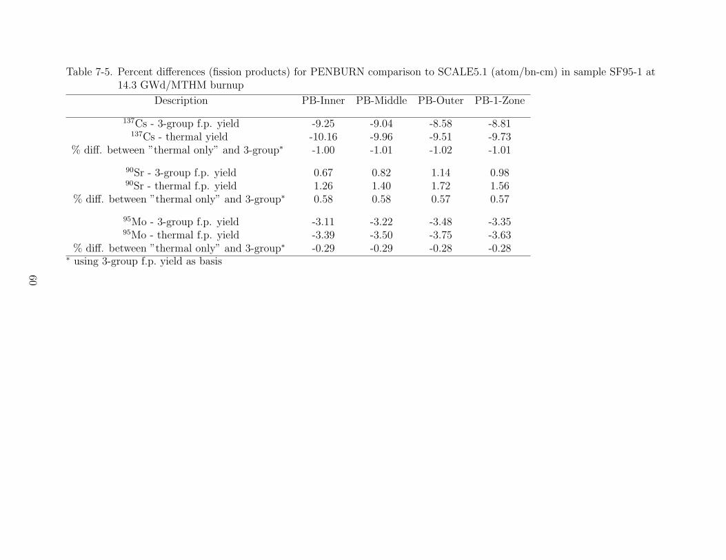
Table 7-5. Percent differences (fission products) for PENBURN comparison to SCALE5.1 (atom/bn-cm) in sample SF95-1 at14.3 GWd/MTHM burnup
Description PB-Inner PB-Middle PB-Outer PB-1-Zone
137Cs - 3-group f.p. yield -9.25 -9.04 -8.58 -8.81137Cs - thermal yield -10.16 -9.96 -9.51 -9.73
% diff. between ”thermal only” and 3-group∗ -1.00 -1.01 -1.02 -1.01
90Sr - 3-group f.p. yield 0.67 0.82 1.14 0.9890Sr - thermal f.p. yield 1.26 1.40 1.72 1.56
% diff. between ”thermal only” and 3-group∗ 0.58 0.58 0.57 0.57
95Mo - 3-group f.p. yield -3.11 -3.22 -3.48 -3.3595Mo - thermal f.p. yield -3.39 -3.50 -3.75 -3.63
% diff. between ”thermal only” and 3-group∗ -0.29 -0.29 -0.28 -0.28∗ using 3-group f.p. yield as basis
60

CHAPTER 8CONCLUSION
We briefly described important aspects of the PENBURN code and its current
coupling to the PENTRAN parallel Sn code. We also demonstrated the capabilities of
PENBURN alongside another burnup code, SCALE5.1, and also with real data based
isotopic mass-spectrometry data obtained following PIE. In doing so, we demonstrated
that for a unit cell PWR problem, PENBURN generated actinides that were, in general,
very accurate compared to PIE mass spectrometry fuel data. Also, accurate comparisons
were revealed for select fission products in comparing SCALE5.1 and PENBURN using
the model based on the same unit cell PWR problem, also incorporating a study of fission
product yield utilization. It was determined that for a thermal PWR system at low
burnups, using only thermal yields versus using 3-group fission yields minimally impacted
nuclide concentrations in atoms/bn-cm by no more than 1 percent for a limited set of
nuclides. Comparisons with SCALE5.1 were similar, although differences in keff values
were attributed to transport differencing methods. This is being investigated further. In
addition, fuel self-shielding was readily apparent, as expected. Also, we demonstrated the
multi fuel-zone adaptability for a radially segmented fuel pin; in PENBURN, both axial
and radial zoning can be performed in 3-D models.
Overall, PENBURN has potential use for tracking radial burnup effects in segmented
fuel zones. The benchmark comparison to SFCOMPO (with necessary assumptions on
power history) serves to illustrate the code’s effectiveness in properly tracking actinide
burnup. In tandem with PENTRAN, the BURNDRIVER sequence enables extensible,
zone-based nuclide tracking in a direct Bateman depletion/burnup solver with 3-D parallel
Sn transport.
Also, PENBURN has a full capability of tracking nuclides in arbitrarily assigned
zones, and has been extended to a 3-D PWR assembly model [23].
61
CHAPTER 9FUTURE WORK
Ultimately, the design of PENBURN/PENTRAN suite (or BURNDRIVER sequence)
is primarily suited for extension to support analysis of single pin fuel transmutation
studies. However, the prowess of PENBURN is in capabilities for analysis performed with
full-sized PWR and BWR assemblies.
With the continual improvement of PENBURN, several features that should be
incorporated are listed:
• Since PENBURN is independent of PENTRAN, it is feasible to gather reaction rateinformation from Monte Carlo codes (e.g. MCNP5) so that the Monte Carlo can actas the transport solver in the BURNDRIVER sequence.
• Improvement of the BURNDRIVER should be performed to have an adaptiveburn step (similar to SCALE5.1’s NEWT/TRITON). A ”predictor-corrector”method/option should be implemented into the driver.
• Also, PENBURN should increase format output capabilities to units of activity, andhave an ability to suppress specific nuclide output.
• An issue with mass defect occurs with transmutation of major actinides into smallerfission products. Since not all fission products are represented in the code, a slightmass defect in the entire fuel occurs that is proportional to burnup. A residualfission product named ’fissium’ should act as the place-holder for the (very small)mass difference from the original fuel.
• Fission product yield utilization (3-group versus thermal only) should be exploredfurther for strongly epithermal and fast fuel systems, where the effect of neglectingfast and epithermal yields (as is often the case) can be measured for variousburnups and systems. While a quick look at on fission product yield utilizationwas performed for a PWR fuel cell at 14.3 GWD/MTHM, more studies that accountfor burnup dependent cross sections should examine lengthier burnups, to at least˜60 GWD/MTHM.
62

APPENDIX ADERIVATION OF THE BATEMAN EQUATION BY LAPLACE TRANSFORMS
The following discussion and equations are strictly adherent to the methodology
exercised in the Nuclear Chemical Engineering text[6]. The derivation is provided because
the Bateman Equation is fundamental for direct solution methods in PENBURN.
A.1 Definition of Laplace Transform
The laplace transform is defined in A–1.
L(t → s) =
∞∫
0
e−stf(t) = f (A–1)
Two essential properties of include a definition of the derivative and the Laplace
transform of an exponential function.
df
dt= −f(0) + sf (A–2)
L[e−λt] =1
s + λ(A–3)
A.2 Derivation of Bateman Equation
The derivation begins with the generalization of a single radioactive decay chain with
initial conditions such that only the first nuclide has a finite number of atoms (the others
assumed not to have any atoms to begin with) at the initial time.
N1 → N2 → N3 → · · · → Ni (A–4)
63

The above amounts to a series of first order differential equations. We shall limit our
examination to the 1st, 2nd, and ith case:
dN1
dt= −λiNi (A–5)
dN2
dt= λ1N1 − λ2N2 (A–6)
dNi
dt= λi−1Ni−1 − λiNi (A–7)
The Laplace transform of these equations are taken, and solved for N , defined as the
transform of N.
N1 =N0
1
λ1 + s(A–8)
N2 =λ1N
01
(λ1 + s)(λ2 + s)(A–9)
Ni =λi−1Ni−1
λi + s=
i−1∏
k=1
λkN01
i∏
k=1
(λk + s)
(A–10)
For brevity, an equivalent expression to A–10 can be developed by partial fraction
expansion:
Ni = N01 λ1λ2 . . . λi−1
i∑j=1
1i∏
k=1k 6=j
(λk − λj)
1
λj + s(A–11)
64
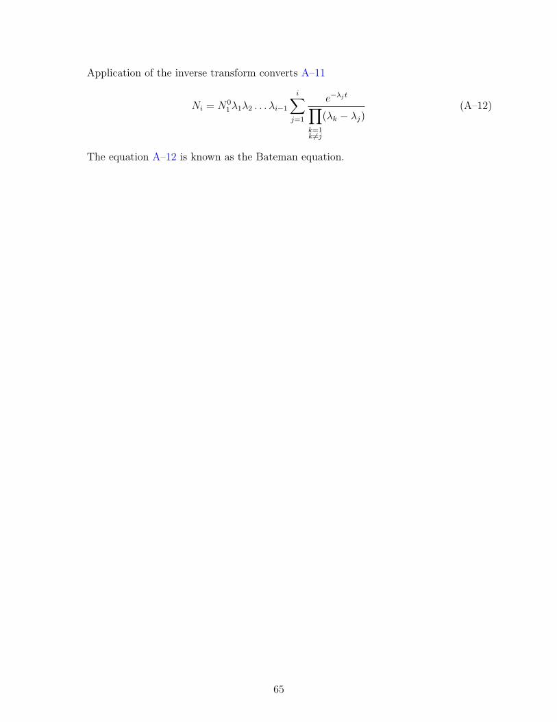
Application of the inverse transform converts A–11
Ni = N01 λ1λ2 . . . λi−1
i∑j=1
e−λjt
∏
k=1k 6=j
(λk − λj)(A–12)
The equation A–12 is known as the Bateman equation.
65

APPENDIX BSOFTWARE INPUT OUTPUT DIAGRAM
• penpow.inp - The penpow.inp file tracks the assignment of fuel materials andrelevant cross section parameters.
Figure B-1. Sample penpow.inp input file
66
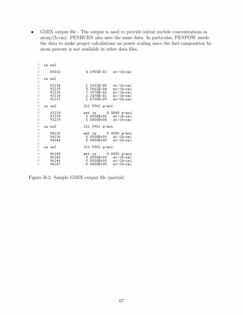
• GMIX output file - The output is used to provide initial nuclide concentrations inatom/(b-cm). PENBURN also uses the same data. In particular, PENPOW needsthe data to make proper calculations on power scaling since the fuel composition byatom percent is not available in other data files.
Figure B-2. Sample GMIX output file (partial)
67

• prbname.crs - Coarse mesh summary data is available through running PENDATA,which provides text files of binary PENTRAN flux data. This file is particularlyuseful for PENPOW as it provides fine mesh volumes. PENPOW uses this file alongwith the flux data in the flx folder to identify and calculate the total fuel volume andmass. In the same manner, the zone fuel flux can be calculated.Note that the fluxes within the coarse mesh summary are not used, as averagingperformed over an entire coarse mesh can incorporate the moderator and clad.Hence, such values are inappropriate when trying to calculate reaction rates and pinpowers.
Figure B-3. Sample coarse mesh summary output file (partial, columns truncated)
68

• prbname.xs - Macroscopic Cross Section File
Figure B-4. Sample macroscopic cross section file (partial)
• prbname.xsc - Microscopic Cross Section File
Figure B-5. Sample microscopic cross section file (partial)
69
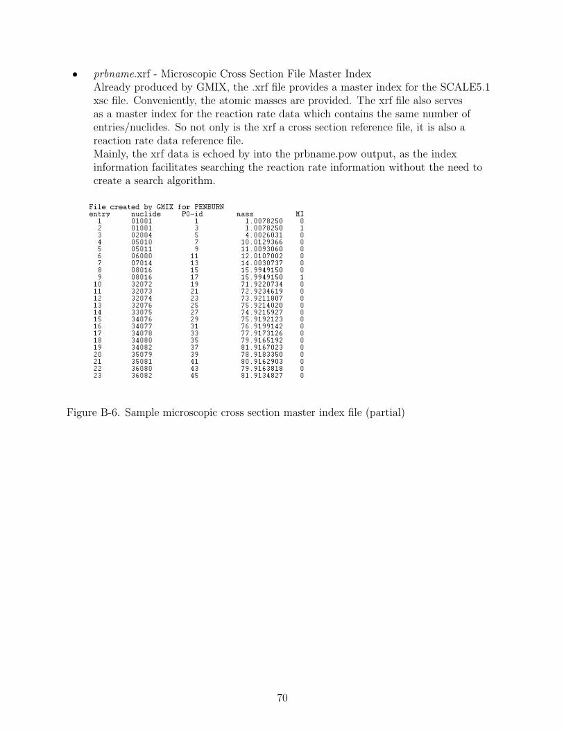
• prbname.xrf - Microscopic Cross Section File Master IndexAlready produced by GMIX, the .xrf file provides a master index for the SCALE5.1xsc file. Conveniently, the atomic masses are provided. The xrf file also servesas a master index for the reaction rate data which contains the same number ofentries/nuclides. So not only is the xrf a cross section reference file, it is also areaction rate data reference file.Mainly, the xrf data is echoed by into the prbname.pow output, as the indexinformation facilitates searching the reaction rate information without the need tocreate a search algorithm.
Figure B-6. Sample microscopic cross section master index file (partial)
70

• prbname.grp - Upper-bound Group Energy File The energy group file, prbname.grp,has already been required by GMIX. Therefore, the user should just copy andpaste this file into the inp directory. A quick examination of the group file showsthe definition of the energy groups and the upper energy cutoffs specified in MeV.A variant of this file is echoed into the prbname.pow output because PENBURNrequires this information.
Figure B-7. Sample upper-bound group energy file
• prbname#.flx files - Scalar Flux Files by energy group number (#). Only one file isprovided as an example.
Figure B-8. Sample group flux file (partial)
71
• prbname.log - The prbname.log file in PENPOW is set up such that only file opensuccesses are recorded. That is, if the user experiences a failure due to a missing orimproperly named file, the log file will only indicate the attempt to open a file andnot report a statement of ”file successfully opened”. The evaluator is encouraged tolook at this file as a diagnostic tool.
• prbname.irm - The .irm file is provided as an intermediate diagnostic output file,which reports the microscopic cross sections, where the fission cross sections arecalculated. Also, the alpha (capture to fission) value and capture fractions arereported.
72
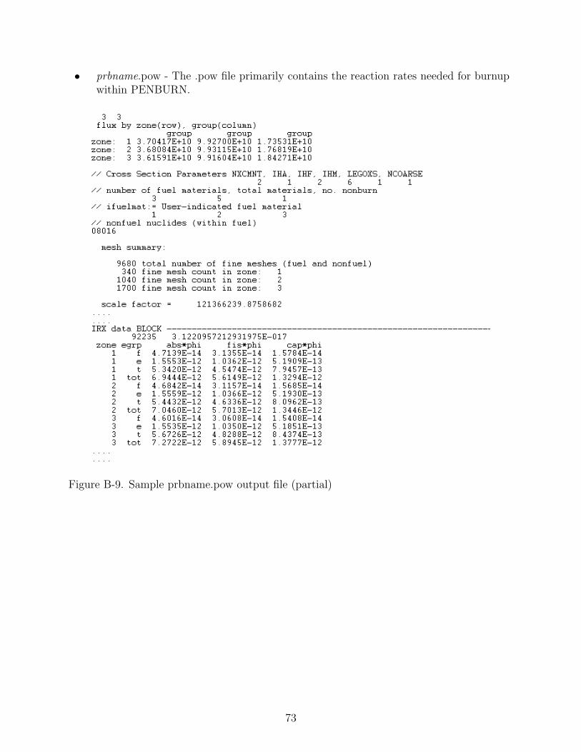
• prbname.pow - The .pow file primarily contains the reaction rates needed for burnupwithin PENBURN.
Figure B-9. Sample prbname.pow output file (partial)
73

• penburn.inp - This is the main, user defined input file for PENBURN.The user is expected to define the following:1. A problem header2. System power in watts (W) or in watts/gram (W/g) using a minus sign before
the number.3. A GMIX keyword (used to differentiate multiple GMIX files for multiple cycles)4. GMIX Output Filename5. Print Option: 1 or 26. Base time (convenient after re-performing transport)7. Irradiation decay times: the first row assigns the number of stages (an
irradiation or decay stage), the successive rows define each stage.
Figure B-10. Sample penburn.inp Input file
74

• penburn.path - The path matrix and map definitions are included within this file.Also, the fission product yield data for over 31 fissile parents is included in the FPYdata BLOCK.
Figure B-11. Sample penburn.path input file
• prbname.log2 - The .log2 file is another diagnostic tool. The extension was notnamed .log as this name is already taken by the PENPOW .log file so as to avoidconfusion. The .log2 file generally indicates whether or not a file was successfullyread, opened, or written. Note that only successful operations are recorded, so ifthere is a missing or corrupt file, it is not reported in the .log2 file.The .log2 file also reports when reaction rate data is missing; if reaction rate datais missing for a particular nuclide the reaction rates are set to zero (implying thatthe capture cross sections are zero). Also, there are extensive fission product yieldavailability reports, which detail the fission percent yields of the fission productsbased on their parent fissile nuclides.
75
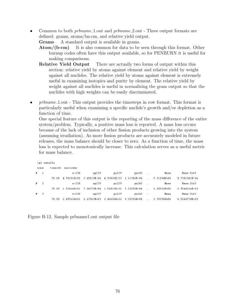
• Common to both prbname 1.out and prbname 2.out - Three output formats aredefined: grams, atoms/bn-cm, and relative yield output.Grams A standard output is available in grams.Atom/(b-cm) It is also common for data to be seen through this format. Other
burnup codes often have this output available, so for PENBURN it is useful formaking comparisons.
Relative Yield Output There are actually two forms of output within thissection: relative yield by atoms against element and relative yield by weightagainst all nuclides. The relative yield by atoms against element is extremelyuseful in examining isotopics and purity by element. The relative yield byweight against all nuclides is useful in normalizing the gram output so that thenuclides with high weights can be easily discriminated.
• prbname 1.out - This output provides the timesteps in row format. This format isparticularly useful when examining a specific nuclide’s growth and/or depletion as afunction of time.One special feature of this output is the reporting of the mass difference of the entiresystem/problem. Typically, a positive mass loss is reported. A mass loss occursbecause of the lack of inclusion of other fission products growing into the system(assuming irradiation). As more fission products are accurately modeled in futurereleases, the mass balance should be closer to zero. As a function of time, the massloss is expected to monotonically increase. This calculation serves as a useful metricfor mass balance.
Figure B-12. Sample prbname1.out output file
76

• prbname 2.out - This output provides the nuclides in row format. This format iscommonly seen with SCALE output.
Figure B-13. Sample prbname2.out output file
77

Figure B-14. Software file input and output diagram for PENPOW and PENBURN codes
78

REFERENCES
[1] A. Vasiliev, H. Ferroukhi, M. A. Zimmermann, and R. Chawla, “Development of aCASMO-4/SIMULATE-3/MCNPX calculation scheme for PWR fast neutron fluenceanalysis and validation against RPV scraping test data,” pp. 615–627, 2007.
[2] G. W. McKinney and E. al., “MCNPX 2.6.X Features (2006-2007),” in M&C SNA2007 Conference Workshop, Monterrey, CA, 2007.
[3] A. L’Abbate, T. Courau, and E. Dumond, “Monte Carlo Criticality Calculations:Source Convergence and Dominance Ratio in an Infinite Lattice Using MCNP andTRIPOLI4,” 2007.
[4] G. Bell and S. Glasstone, Nuclear Reactor Theory. New York: Van NostrandReinhold, 1970.
[5] E. M. Baum, H. D. Knox, and T. R. Miller, “Nuclides and Isotopes: Chart of theNuclides,” Lockheed Martin, Tech. Rep., 2002.
[6] M. Benedict, T. H. Pigford, and H. W. Levi, Nuclear Chemical Engineering, 2nd ed.McGraw Hill, 1981.
[7] J. Cetnar, “General solution of Bateman equations for nuclear transmutations,”Annals of Nuclear Energy, vol. 33, no. 7, pp. 640–645, 2006.
[8] A. I. Shlyakhter, “Depletion functions and their use in the calculation of isotopetransmutations,” p. 6, 1983.
[9] T. R. England and B. F. Rider, “Evaluation and Compilation of Fission ProductYields,” Los Alamos National Laboratory, Tech. Rep., 1993.
[10] J. J. Duderstadt and L. J. Hamilton, Nuclear Reactor Analysis. Canada: HamiltonPrinting Company, 1976.
[11] R. E. MacFarlane and D. W. Muir, “The NJOY Nuclear Data Processing System,Version 99,” Los Alamos National Laboratory, Tech. Rep., 1999.
[12] T. Mock, “Tandem Use of Monte Carlo and Deterministic Method for Analysis ofLarge Scale Heterogeneous Radiation Systems,” Master’s thesis, University of Florida,2007.
[13] W. B. Wilson, T. R. England, D. C. George, D. W. Muir, and P. G. Young, “Recentdevelopment of the CINDER‘90 transmutation code and data library for actinidetransmutation studies,” Los Alamos National Laboratory, Tech. Rep., 1995.
[14] E. Romanov, V. Tarasov, and F. Vahetov, “ORIPXXI Computer Programs forIsotope Transmutation Simulations,” 2005.
[15] E.G. Romanov, ”ChainSolver”, http://snow.prohosting.com/roeug/ChainSolver.htm.[Online]. Available: http://snow.prohosting.com/roeug/ChainSolver.htm
79
[16] SCALE: A Modular Code System for Performing Standardized Computer Analyses forLicensing Evaluation. Oak Ridge: ORNL, vol. I, II, and III.
[17] J. T. Long, Engineering for Nuclear Fuel Reprocessing. Gordon and Breach, 1967.
[18] M. D. DeHart, “Simplification of Multigroup Cross-Section Processing for LargeDepletion Calculations in Triton,” in Proceeding of the Joint International Conferenceon Mathematical Methods and Supercomputing for Nuclear Applications, Monterrey,CA, 2007.
[19] G. Sjoden and A. Haghighat, “PENTRAN - A 3-D Cartesian Parallel SN Code withAngular, Energy, and Spatial Decomposition,” in Proceedings of the Joint InternalConference on Mathemtical Methods and Supercomputing for Nuclear Applications,vol. I, Saratoga Springs, NY, 1995, p. 553.
[20] H. Mochizuki, K. Suyama, Y. Nomura, and H. Okuno, “Spent Fuel CompositionDatabase System on WWW - SFCOMPO on WWW Ver. 2,” Japan Atomic EnergyResearch Institute, Tech. Rep., 2001, JAERI-Data/Code 2001-020.
[21] B. Roque, P. Marimbeau, and J. P. Grouiller, “Depletion Calculation BenchmarkDeveoted to Fuel Cycle Issues - Specification for Phase I,” 2004, NEA/NS/DOC(2004)11Unclassified.
[22] M. D. DeHart, I. C. Gauld, and M. L. Williams, “High-fidelity Lattice PhysicsCalculations of the SCALE Code System Using TRITON,” in Proceedings of the JointInternational Conference on Mathematical Methods and Supercomputing for NuclearApplications, Monterrey, CA, 2007.
[23] T. Plower, K. Manalo, M. Rowe, and G. Sjoden, “Fuel burnup analysis of a 17X17PWR assembly using the PENTRAN/PENBURN suite,” in PHYSOR’08:InternationalConference on the Physics of Reactors ”Nuclear Power: A Sustainable Resource”.
80

BIOGRAPHICAL SKETCH
Kevin Manalo earned a B.S. in nuclear engineering from the University of Florida
in May 2006. Thereafter, Kevin remained at the University of Florida to earn an M.S. in
nuclear engineering. Kevin Manalo and Mi Huang married during the month of March
2008. Upon completion of the M.S. program, Kevin will remain at the University of
Florida to pursue his Ph.D. studies.
81