dhana wang cfd mist 180 bend ihtc 5-28-2010 final...

Copyright © 2010 by ASME 1

Proceedings of the International Heat Transfer Conference IHTC14

August 8-13, 2010, Washington, DC, USA

IHTC14-22833

CFD Model Validation and Prediction of Mist/Steam Cooling in a 180-Degree Bend Tubes

T. S. Dhanasekaran and Ting Wang

Energy Conversion and Conservation Center University of New Orleans

New Orleans, Louisiana, USA

ABSTRACT To achieve higher efficiency target of the advanced turbine systems, the closed-loop steam cooling scheme is employed to cool the airfoil. It is proven from the experimental results at laboratory working conditions that injecting mist into steam can significantly augment the heat transfer in the turbine blades with several fundamental studies. The mist cooling technique has to be tested at gas turbine working conditions before implementation. Realizing the fact that conducting experiment at gas turbine working condition would be expensive and time consuming, the computational simulation is performed to get a preliminary evaluation on the potential success of mist cooling at gas turbine working conditions. The present investigation aims at validating a CFD model against experimental results in a 180-degree tube bend and applying the model to predict the mist/steam cooling performance at gas turbine working conditions. The results show that the CFD model can predict the wall temperature within 8% of experimental steam-only flow and 16% of mist/steam flow condition. Five turbulence models have been employed and their results are compared. Inclusion of radiation into CFD model causes noticeable increase in accuracy of prediction. The reflect Discrete Phase Model (DPM) wall boundary condition predicts better than the wall-film boundary condition. The CFD simulation identifies that mist impingement over outer wall is the cause for maximum mist cooling enhancement at 450 of bend portion. The computed results also reveals the phenomenon of mist secondary flow interaction at bend portion, adding the mist cooling enhancement at the inner wall. The validated CFD simulation predicts that average of 100% mist cooling enhancement can be achieved by injecting 5% mist at elevated GT working condition. Keywords: Mist cooling, heat transfer enhancement, two-phase flow, gas turbine blade cooling INTRODUCTION Several major gas turbine manufacturers have adopted closed-loop steam cooling for their heavy-frame advanced turbine systems (ATS) engines ([1-3]). The air film cooling can be eliminated by taking advantage of the closed-loop

steam cooling scheme in a combined cycle system [4]. As the turbine inlet temperature is raised to 14000C, excessive film cooling is the major obstacle to a further increase in gas turbine thermal efficiency (Bannister [5]). The aerodynamic and thermal losses could occur due to interference of cooling air injected from the airfoil into the main hot gas flow. On the other hand, less air is available for combustion and therefore the work output will be reduced. Furthermore, excessive film cooling will force the combustion temperature to be raised in order to achieve higher turbine inlet temperature and further compound the issue of reducing NOx and controlling emissions. One of the challenging problems of employing closed-loop steam cooling is the requirement of diverting a large amount of steam to cool the turbine vanes and blades [3 and 6]. In order to eliminate film cooling, the coolant side heat transfer coefficient must be greatly increased (to about 8,000 – 10,000 W/m2K). To reach such high heat transfer coefficients, a very high steam Reynolds number (thus a very high steam flow rate) must be maintained. Drawing this large amount of steam out from the bottom steam cycle would decrease the thermal efficiency of the bottom steam turbines since the normal steam expansion process would be interrupted [7]. Furthermore, high steam rate will significantly increase the pressure losses. To address the above issues, the concept of controlled closed-loop mist/steam cooling was introduced and verified with extensive basic experiments on a horizontal tube [8,9], a 180-degree curved tube [10], impingement jets on a flat surface [11], and impingement jets on a curved surface [12]. Typically, an average cooling enhancement of 50 - 100% was achieved by injecting 1-3% (wt.) mist into the steam flow. Very high local cooling enhancement of 200 - 300% was observed in the tube and on a flat surface, and cooling enhancement above 500% was observed when steam flow passed the 180-degree bend. The experimental and numerical heat transfer results of spray cooled air-mist flows around cylinders [13-14], wedge-shaped bodies [15] and plates [16-17] have also shown the predominant effect of mist in the cooling enhancement. Similar effects have been observed in the post dryout vapour-droplet flow in the duct [18-19]. The spray cooled air-mist flows and post dryout vapour-droplet flows


are different from the current study of controlled mist/steam dispersed flow. The main difference between the post-dryout dispersed flow and the present mist/steam flow is that they have different inlet conditions. The droplet size and distribution as well as the liquid mass fraction at the critical heat flux point for post-dryout flow depend on the flow conditions prior to the critical heat flux point and are usually difficult to control. The inlet conditions for the mist/steam internal flow in the present study are controlled mainly by the atomizing system, the droplet size and distribution as well as the liquid mass fraction and liquid temperature can be systematically controlled. The mist droplets are suspended in the flow and are transported by the flow medium via drag; whereas the droplets in the spray flow are transported by the droplets inertia. The droplets in the post-dryout flow are usually generated from the breakup and entrainment of liquid layers and the droplet sizes are quite large. Similarly, impinging liquid spray cooling involves liquid evaporation and bears some similarity to mist impinging cooling, but the liquid droplets in the spraying cooling are typically very large (50μm - 2 mm) and are transported dominantly by droplets inertia with minimal entrained gas flow. Therefore, the two-phase flow physics and flow field of liquid spray cooling are different from mist impinging jet cooling. More detailed literature reviews on mist/steam cooling can be found in Guo et al.[8] and Li et al. [11]. Though the experimental investigations showed promising performance of mist/steam cooling, keeping in mind that the gas turbines are designed to operate at high temperature and high pressure conditions, the concept has to be tested at such elevated conditions before it can be implemented with confidence. Realizing the difficulties in conducting experiments in gas turbine working conditions, the present study focuses on validating the CFD model with the experimental data taken in the laboratory in a 180 degrees bend tube by Guo et al. [10] and followed by using this validated CFD model to predict the mist/steam performance under elevated gas turbine temperature and pressure conditions. This study is a part of our continuous effort on validating mist/steam CFD model for various conditions. The validation results for impinging jet and horizontal tube models can be found in Dhanasekaran and Wang [20-21].

The mist/steam experimental results by Guo et al. [10] showed that the outer wall of 180-degree bend had a better cooling than the inner wall for both steam and mist/steam cases. They revealed that the mist-cooled outer wall had a maximum cooling at 450 location and speculated that this enhancement was caused by the direct mist impingement on the outer wall due to inertia of water droplets coming from the upstream straight section and centrifugal force. Their experimental results also showed that the average mist cooling enhancement reached 200-300% under lower heat flux conditions, but it deteriorated to about 50 % under higher heat flux conditions. It was concerned then that the mist cooling might not be beneficial under the elevated wall heat flux condition in the real gas turbine operating

environment. However, they further increased the Reynolds number and observed the cooling enhancement returning back to above 100%. Based on this finding, Guo et al. [9] hypothesized that the mist cooling could be still attractive under elevated gas turbine operating condition because the Reynolds number is high and the steam properties will change in favor of mist cooling in the actual gas turbine environment.

The objective of this paper is to investigate whether their hypothesis is correct by validating a CFD model with their experimental results and then apply the validated CFD model to predict the potential mist/steam cooling under actual gas turbine operating conditions.

2. EXPERIMENTAL SET-UP AND NUMERICAL MODEL 2.1 Test Section

Figure 1a shows the experimental test section employed by Guo et al. [10]. As shown in the figure, the steam enters through 132mm of heated pipe before entering 180o bend tube and exists through 203mm length heated pipe. The unheated tube is used to transport the steam from mixing chamber to the bend test tube and further to the condenser. The tube inside diameter is 20.5mm and the bending radius is 57mm (from origin to center of pipe). The test section was placed horizontally and was directly heated by a high-current power supply system. Additional details on the experimental test set-up can be obtained from Guo et al. [10]. The geometry details and computational domain considered are shown in Fig. 1b. The unheated pipe length of 78mm was considered to achieve the fully developed flow as in the experimental case.

It should be noted that the mist was not generated by an atomizer near the tube entrance; rather, the mist was generated and mixed with saturated steam in a mixer approximate 3 feet away from the test section. This process provides a true mist flow with liquid droplets suspending in the main flow, which is different from a sprayed flow. In a sprayed flow, the inertia of the liquid droplets dominate, whereas in a mist flow the droplets are relatively more passive and transported by the gas flow. It should be noted that no rotating effect is included in the experimental study, so the results of this study can be applied to vane cooling, but require modification by including the rotating effect before they can be more accurately applied to the rotating blades.


Flow inlet

Flow outlet

Heated portion (q’’ = 14,500 W/m2) Unheated portion

132 78

2037

0o

45o

180o

All dimensions are in mm

57 20.5

(a)

(b)

z x

135o

90o

Figure 1. a) Experimental set-up [10] and b) CFD computational domain. 2.2 Numerical Method

A feasible method to simulate the steam flow with mist injection is to consider the droplets as a discrete phase since the volume fraction of the liquid is usually small (e.g. 5% mist by weight gives approximately 0.08% in volume.) The trajectories of the dispersed phase (droplets) are calculated by the Lagrangian method by tracking each droplet from its origin. The impact of the droplets on the continuous phase is considered as source terms to the governing equations of mass, momentum and energy. Two components (water and water vapor) are simulated in this tube flow. 2.2.1 Governing equations The 3-D transient Navier-Stokes equations as well as equations for mass and energy are solved. The governing equations for conservation of mass, momentum, and energy are given as: ( ) mi

i

Sρuxt

=∂∂

+∂ρ∂ (1)

( ) ( ) ( ) jjiijij

jjii

j Fu'u'ρ-τxx

Pgρuρux

ρut

+∂∂

+∂∂

−=∂∂

+∂∂ v (2)

( ) ( ) hipii

ipi

p SμΦT'u'ρc-xTλ

xTuρc

xTρc

t++⎟⎟

⎠

⎞⎜⎜⎝

⎛∂∂

∂∂

=∂∂

+∂∂ (3)

where τij is the symmetric stress tensor defined as

⎟⎟⎠

⎞⎜⎜⎝

⎛

∂∂

−∂∂

+∂

∂=

k

kij

j

i

i

jij x

uδ32

xu

xu

μτ (4)

The source terms (Sm, Fj and Sh) are used to include the contribution from the dispersed phase. μΦ is the viscous dissipation.

In mist/air cooling, water droplets evaporate, and the vapor diffuses and is transported into its surrounding flow. Different from the mist/air flow, no species transport equation is used in the mist/steam flow since steam is the only main flow medium.

The terms of ρ ji u'u' and ρcp T'u'i , represent the Reynolds stresses and turbulent heat fluxes. The bend tube with Reynolds numbers (based on inlet diameter and the inlet condition) 20,000 is considered for this study. 2.2.2 Turbulence model

The standard k-ω model was used in the CFD model. The selection was based on test among other models including standard k-ε, RNG k-ε, Realizable k-ε, and SST k-ω. The constants used in these models follow the recommended values from reference [22]. The standard k-ω model is an empirical model based on transport equations for the turbulent kinetic energy (k) and the specific dissipation rate (ω), which can also be considered as the ratio of ε to k [23]. The low-Reynolds-number effect is accounted for in the k-ω model. The detailed results on effect of the turbulence model are presented in the following section.

2.2.3 Discrete-phase model (Water droplets) 2.2.3.1 Droplet Flow and Heat Transfer Based on Newton’s 2nd law, the droplet motion in the flow can be formulated by

∑= F/vp dtdmp (5)

where vp is the droplet velocity (vector). The right-hand side is the combined force acting on the droplet, which normally includes the hydrodynamic drag, gravity, and other forces such as Saffman's lift force [24], thermophoretic force [25], and Brownian force [26], etc. Saffman force concerns a sphere moving in a shear field. It is perpendicular to the direction of flow, originating from the inertia effects in the viscous flow around the particle. It can be given as:

0.5pg

0.5saff )(du/dn)u(u1.615ρF −= ν (6)

where du/dn is the gradient of the tangential velocity. It is valid only when Rep<<1.

The thermophoretic force arises from asymmetrical interactions between a particle and the surrounding fluid molecules due to temperature gradient. This force tends to repel particles or droplets from a high temperature region to a low temperature region. The following equation can be used to model this force:


nT

Tm1KFp

n ∂∂

−= (7)

More details can be found in Talbot et al. [25]. Brownian force considers the random motion of a small

particle suspended in a fluid, which results from the instantaneous impact of fluid molecules. It can be modeled as a Gaussian white noise process with spectral intensity given by [26]. All the three forces are included in the CFD model. Our previous investigation on impingement [20] identified saffman force as important force among other two forces should be considered with main forces of drag and gravity to improve the accuracy of CFD model.

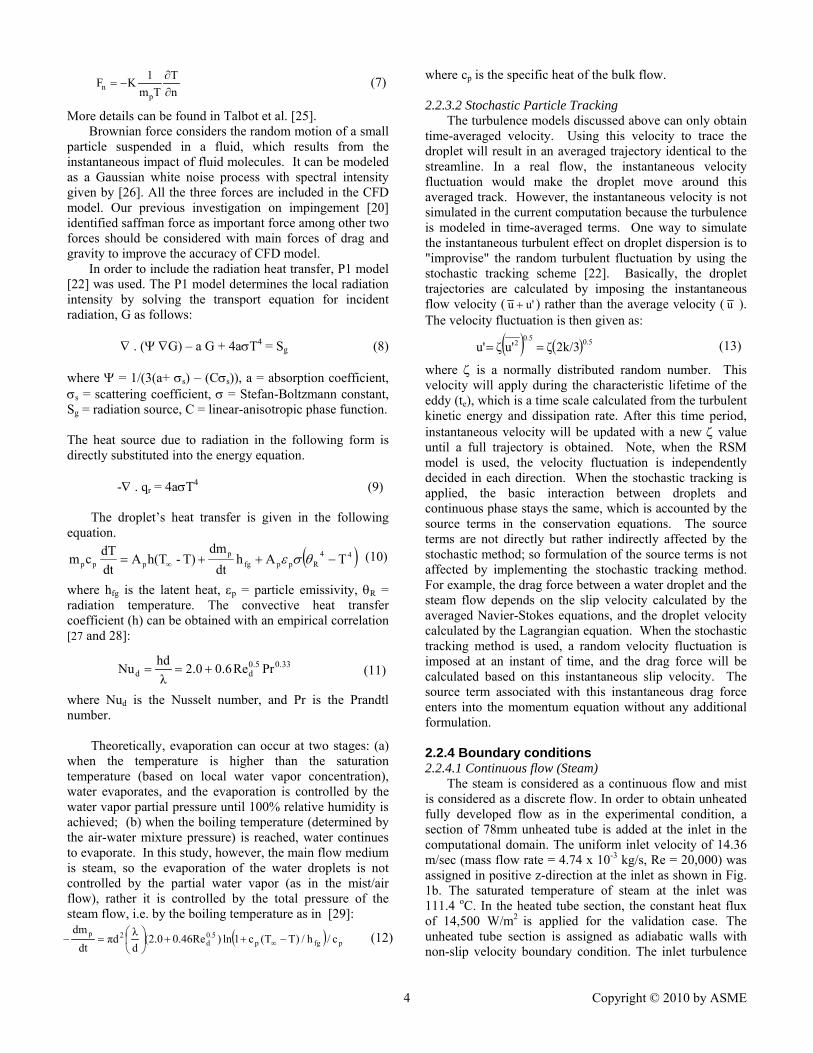
In order to include the radiation heat transfer, P1 model [22] was used. The P1 model determines the local radiation intensity by solving the transport equation for incident radiation, G as follows: ∇ . (Ψ ∇G) – a G + 4aσT4 = Sg (8) where Ψ = 1/(3(a+ σs) – (Cσs)), a = absorption coefficient, σs = scattering coefficient, σ = Stefan-Boltzmann constant, Sg = radiation source, C = linear-anisotropic phase function. The heat source due to radiation in the following form is directly substituted into the energy equation. -∇ . qr = 4aσT4 (9) The droplet’s heat transfer is given in the following equation.

( )44Rppfg

pppp TAh

dtdm

T)-h(TAdtdTcm −++= ∞ θσε (10)

where hfg is the latent heat, εp = particle emissivity, θR = radiation temperature. The convective heat transfer coefficient (h) can be obtained with an empirical correlation [27 and 28]:

33.05.0dd PrRe6.00.2

λhdNu +== (11)

where Nud is the Nusselt number, and Pr is the Prandtl number.

Theoretically, evaporation can occur at two stages: (a) when the temperature is higher than the saturation temperature (based on local water vapor concentration), water evaporates, and the evaporation is controlled by the water vapor partial pressure until 100% relative humidity is achieved; (b) when the boiling temperature (determined by the air-water mixture pressure) is reached, water continues to evaporate. In this study, however, the main flow medium is steam, so the evaporation of the water droplets is not controlled by the partial water vapor (as in the mist/air flow), rather it is controlled by the total pressure of the steam flow, i.e. by the boiling temperature as in [29]:

( ) pfgp0.5d

2p c/h/)TT(c1ln)0.46Re(2.0dλπd

dtdm

−++⎟⎠⎞

⎜⎝⎛=− ∞ (12)

where cp is the specific heat of the bulk flow. 2.2.3.2 Stochastic Particle Tracking

The turbulence models discussed above can only obtain time-averaged velocity. Using this velocity to trace the droplet will result in an averaged trajectory identical to the streamline. In a real flow, the instantaneous velocity fluctuation would make the droplet move around this averaged track. However, the instantaneous velocity is not simulated in the current computation because the turbulence is modeled in time-averaged terms. One way to simulate the instantaneous turbulent effect on droplet dispersion is to "improvise" the random turbulent fluctuation by using the stochastic tracking scheme [22]. Basically, the droplet trajectories are calculated by imposing the instantaneous flow velocity ( u' u + ) rather than the average velocity ( u ). The velocity fluctuation is then given as:

( ) ( )0.50.52 2k/3ζu'ζu' == (13)

where ζ is a normally distributed random number. This velocity will apply during the characteristic lifetime of the eddy (te), which is a time scale calculated from the turbulent kinetic energy and dissipation rate. After this time period, instantaneous velocity will be updated with a new ζ value until a full trajectory is obtained. Note, when the RSM model is used, the velocity fluctuation is independently decided in each direction. When the stochastic tracking is applied, the basic interaction between droplets and continuous phase stays the same, which is accounted by the source terms in the conservation equations. The source terms are not directly but rather indirectly affected by the stochastic method; so formulation of the source terms is not affected by implementing the stochastic tracking method. For example, the drag force between a water droplet and the steam flow depends on the slip velocity calculated by the averaged Navier-Stokes equations, and the droplet velocity calculated by the Lagrangian equation. When the stochastic tracking method is used, a random velocity fluctuation is imposed at an instant of time, and the drag force will be calculated based on this instantaneous slip velocity. The source term associated with this instantaneous drag force enters into the momentum equation without any additional formulation. 2.2.4 Boundary conditions 2.2.4.1 Continuous flow (Steam)

The steam is considered as a continuous flow and mist is considered as a discrete flow. In order to obtain unheated fully developed flow as in the experimental condition, a section of 78mm unheated tube is added at the inlet in the computational domain. The uniform inlet velocity of 14.36 m/sec (mass flow rate = 4.74 x 10-3 kg/s, Re = 20,000) was assigned in positive z-direction at the inlet as shown in Fig. 1b. The saturated temperature of steam at the inlet was 111.4 oC. In the heated tube section, the constant heat flux of 14,500 W/m2

is applied for the validation case. The unheated tube section is assigned as adiabatic walls with non-slip velocity boundary condition. The inlet turbulence


intensity is specified as 2%. The flow exit of computational domain is assumed to be at a constant pressure of 1.0 atm. Variable properties are assigned as a function of temperature and pressure. 2.2.4.2 Discrete flow (mist)

The fine water droplets with distributed droplet diameters are considered. The droplets varying from 1 μm to 30 μm with the mean diameter of about 6μm were reported in the experimental studies [10]. In the simulation, the Rosin-Rammler distribution function is used which is based on the assumption that an exponential relationship exits between the droplet diameter, dd, and the mass fraction of droplets with diameter greater than d, Yd:

nmdd

d eY )/(−= (14) where dm refers to the mean diameter and n refers to the spread parameter. From the relationship, the spread parameter (2.4) is calculated and used to fit the size distribution into the CFD model. A total number of 2350 injection locations are deployed at the inlet. A mass concentration ratio (mist/steam) of 3% was assigned for validation case. 2.2.4.3 Discrete phase wall boundary condition

When the droplet reaches the wall, the droplet trajectory is determined from the discrete phase wall boundary condition. Each droplet when it approaches the wall can undergo one of the several possible mechanisms based on the condition of the wall: dry or flooded.

In case of dry wall (Fig. 2a), the droplets have three major regimes including reflect, break-up and trap. According to Watchers et al. [30], the regimes depend on the incoming Weber number of the droplet. Here, the Weber number is the ratio of kinetic energy of a droplet to the surface energy of a droplet (We = ρ dd vd

2 /σ). It was shown from the experimental results that the droplet with incoming Weber number (Wein) less than 10 reflects elastically with nearly same outgoing Weber number (Weout). As the incoming We increased further to Wein > 80, the droplet falls into disintegration region which leads breaking-up the droplet to several small droplets. In the transition region of 30<We<80, the droplet has the chance to either reflect or breakup. Apart from the above two phenomena, the droplets can be trapped by the superheated wall also. In this case the trajectory calculations are terminated and particles entire mass instantaneously passes into the vapor phase and enters the cell adjacent to the boundary through the source term (Sm) in the continuity equation (Eq. 1). On the other hand, when the droplets impinge on the flooded wall, it has the chance for four different regimes including splashing, spread, rebound and sticking as shown in Fig. 2b. Harlow and Shannon [31] applied the marker-and-cell (MAC) technique to obtain finite difference solutions to the Navier-Stokes equations for a viscous, incompressible liquid droplet impinging on a flat surface with and without liquid films. Even though the technique captures much of physics of drop-film interactions, it

requires higher computational effort. Bai and Gosman [32] developed a spray impingement model which was formulated on the basis of literature findings and mass, momentum and energy conservation constraints. In their study the secondary droplets resulting from splashing had the distribution of sizes and velocities by analyzing the relevant impingement regimes and the associated post-impingement characteristics. The rebound velocity was calculated from the following equations.

V’td = (5/7) Vtd (15)

V’nd = - e Vnd (16)

where Vtd is the initial tangential velocity, Vnd is the initial normal velocity, V’

td is the rebounding tangential velocity,

V’nd

is the rebounding normal velocity and the expression e is the function of the impingement angle. For the spread regime, the arriving droplets are assumed to coalesce to form a local film. Within the splashing regime, it is assumed that two droplets of equal mass are ejected from the liquid film at a randomly determined in-plane angle. The ratio of mass splashed to the incident droplet mass is randomly determined to vary between 0.2 to 1.1. The total number of splashed droplets is determined from a curve-fit of Stow and Stainer’s [33] data. Using mass conservation the droplet diameters are then determined. The wall film and reflect models are used in this study. The wall film model used in this study is based on the work of Stanton et al. [34] and O’Rourke et al. [35]. The four regimes, stick, rebound, spread, and splash are based on the impact energy and wall temperature. Below the boiling temperature of the liquid, the impinging droplet can either stick, spread or splash, while above the boiling temperature, the particle can either rebound or splash. The impact energy is defined by E2 = (ρ Vr

2 dd / σ ) [1/(min (h0 /dd ,1) + δbl /dd ] (17) where Vr is the relative velocity of particle in the frame of the wall and δbl is the boundary layer thickness. The sticking regime is applied when the value of E becomes less than 16. Splashing occurs when the impingement energy is above a critical E value of Ecr

= 57.7. The splashing algorithm is followed as described in Stanton et al. [34].


Splashing Spread Rebound Sticking

Reflect Break-up Trap

Hot surfaceFour regimes in the flooded wall

Three regimes in the dry wall

becomes vapor

(a)

(b)

Figure 2. Droplet-wall interaction models.

2.2.5 Computational Meshes The computational domain has been discretized to fine cells to conduct the simulation. Figure 3a shows the computational grid of bend tube, which contains hexahedral elements. The total number of 130,000 elements is used in this model. To accurately predict possible recirculation, separation, and reattachment zones, the cells have been clustered towards the wall to obtain appropriate y+ value less than 1. The grid independence test has been carried out and sample result are shown in Fig. 3b. The figure confirms that the wall temperature at outer surface does not change much when number of elements are decreased from 130,000 to 70,000. The computation has been carried out using the commercial CFD software FLUENT (Version 6.3.26) from Ansys, Inc. The 3-D transient simulation uses the pressure-based solver, which employs an implicit pressure-correction scheme and decouples the momentum and energy equations. The SIMPLE algorithm is used to couple the pressure and velocity. Second order upwind scheme is selected for spatial discretization of the convective terms. The second order accuracy is obtained by calculating quantities at cell faces using multidimensional linier reconstruction approach [22]. The transient computation is

conducted for the steam field (continuous phase) first. After obtaining converged and stabilized flow field of the steam, the dispersed phase of droplet trajectories are calculated. At the same time, drag, heat and mass transfer between the droplets and the steam flow are calculated. Variable property values are calculated using piecewise-linear equations for steam and water droplets. It was discovered that the property database for water vapor and steam in FLUENT is not sufficient and gives unreasonable results such as predicting temperature lower than Wet Bulb temperature after water droplet evaporation. A denser database has been incorporated through Function statement.

Iterations proceed alternatively between the continuous and discrete phases. Ten iterations in the continuous phase are conducted between two iterations of the discrete phase. Converged results are obtained after the residuals satisfy mass residual of 10-4, energy residual of 10-6, and momentum and turbulence kinetic energy residuals of 10-5. These residuals are the summation of the imbalance in each cell, scaled by a representative for the flow rate. The computation was carried out in parallel processing on two dual-core Pentium clusters with 16 nodes each. The both steam only and mist/steam simulation results presented here are after stabilization of flow and temperature distribution on the hot wall.

200

220

240

260

280

300

320

340

0 45 90 135 180 225 270 315

Axial Distance

Wal

l tem

pera

ture

( o C

)

Exp, Outer wallCFD, 130,000 elementsCFD, 70,000 elements

(a)

(b)

#1TC #2TC #3TC

Figure 3. (a) Computational grid and an enlarged view at tube inlet and (b) Effect of element numbers.


3. RESULTS AND DISCUSSION 3.1 Validation of CFD model

The CFD model validation against experimental results for steam only and mist/steam cases are presented in this section. Figure 4 shows the wall temperature distribution along inner and outer curved surfaces of the bend tube. The locations selected for measurement [10] are 0, 45, 90, 135 and 180 degrees in the bend section and three downstream locations from the bend section with one diameter of tube distance interval (#TC) as shown in Fig. 1a. It is noticed that the CFD model with radiation predicts better at the curved portion of inner surface (Fig. 4a) and at the downsteam locations, the one without radiation predicts better. Dhanasekaran and Wang [20] showed better validation of their CFD model without inclusion of radiation in horizontal tube arrangement. This shows that the effect of radiation is partially depending on the shape of hot surface.

150

200

250

300

350

400

Wal

l tem

pera

ture

( o C

) Exp, steam only

CFD, with radiation

150

200

250

300

350

400

0 45 90 135 180 225 270 315

Axial Distance

Wal

l tem

pera

ture

( o C

)

Re = 20,000 q’’ = 14,500 W/m2

Std k-ω model

#1TC #2TC #3TC

(a) Outer wall

(b) Inner wall

Figure 4. Effect of radiation in CFD model: (a) outer wall ( b) inner wall (standard k-ω, steady state).

In order to select appropriate turbulence model for this application, various models including standard k-ε, RNG k-ε, Realizable k-ε, standard k-ω and SST k-ω are tested and results are shown in Fig. 5. In the inner wall, all the turbulence models underpredict the wall temperature along the bend, while the standard k-ω model provides the best prediction in the straight wall section downstream the bend

exit. In the outer wall, all three k-ε models predicts the temperature better than the two k-ω models, but none of the turbulence models satisfactorily capture the temperature abrupt increasing trend well. Overall speaking, the standard k-ω model provides a better overall prediction than other models with an average of 13% deviation from the experimental data at outer wall and 3% at inner wall. The deviation is calculated by (Tcfd-Texp)/(Tmax-Tsat), where Tmax is the maximum temperature on the hot wall and Tsat is the saturation temperature. None of the turbulence models tested here could predict the temperature distribution at downstream locations (#1TC, #2TC and #3TC) of outer wall well.

100

150

200

250

300

350

400

0 45 90 135 180 225 270 315

Axial Distance

Wal

l tem

pera

ture

( o C

)

Exp, Outer wallCFD, std k-eCFD, RNG k-eCFD, Rea K-eCFD, std k-wCFD, SST k-w

Re = 20,000 q’’ = 14,500 W/m2

100

150

200

250

300

350

400

0 45 90 135 180 225 270 315

Axial Distance

Wal

l tem

pera

ture

( o C

)

Exp, Inner wallCFD, std k-eCFD, RNG k-eCFD, Rea k-eCFD, std k-wCFD, SST k-w

#1TC #2TC #3TC

(a) Outer wall

(b) Inner wall

Std k-ε RNG k-ε Rea k-ε Std k-ω SST k-ω

Std k-ε RNG k-ε Rea k-ε Std k-ω SST k-ω

Figure 5. Effect of turbulence CFD model: (a) outer wall and (b) inner wall (steady state with radiation).

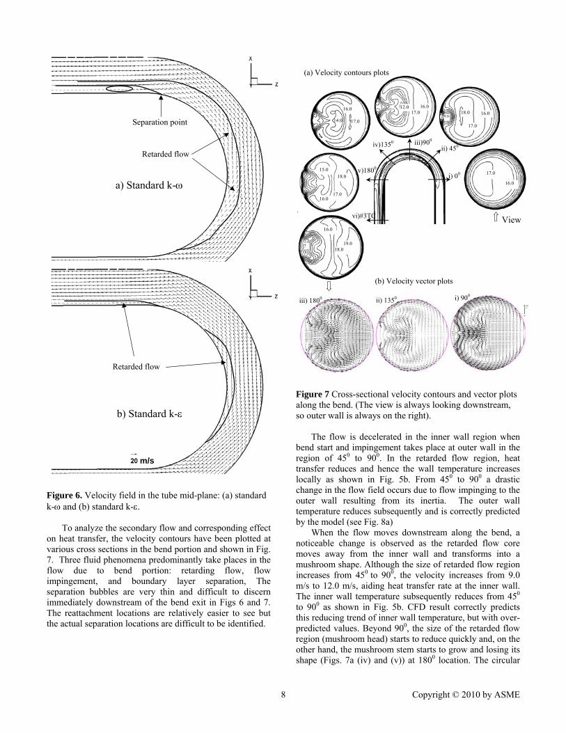
The flow fields calculated by the standard k-ω and standard k-ε models are shown in Fig. 6a and b respectively. The standard k-ω model predicts a regions of flow retardation starting at 100 due to the bend and retains until downstream of the bend. It is speculated that separation occurs in this region of retarded flow, but inspection of near-wall flow doesn't uncover any flow reversal until the straight wall section immediately downstream of the bend exit.


a) Standard k-ω

b) Standard k-ε

Separation point

Retarded flow

m/s

Retarded flow

Figure 6. Velocity field in the tube mid-plane: (a) standard k-ω and (b) standard k-ε.

To analyze the secondary flow and corresponding effect

on heat transfer, the velocity contours have been plotted at various cross sections in the bend portion and shown in Fig. 7. Three fluid phenomena predominantly take places in the flow due to bend portion: retarding flow, flow impingement, and boundary layer separation, The separation bubbles are very thin and difficult to discern immediately downstream of the bend exit in Figs 6 and 7. The reattachment locations are relatively easier to see but the actual separation locations are difficult to be identified.

ii) 450

i) 00

iii)900 iv)1350

17.0 v)1800

16.0

15.0

16.0 17.0

18.0

18.0

17.0

16.0 16.0

17.0 12.0

17.0 14.0

16.0

View

9.0

vi)#3TC

19.0 18.0

16.0

7

(a) Velocity contours plots

(b) Velocity vector plots

i) 900iii) 1800 ii) 1350

Figure 7 Cross-sectional velocity contours and vector plots along the bend. (The view is always looking downstream, so outer wall is always on the right).

The flow is decelerated in the inner wall region when bend start and impingement takes place at outer wall in the region of 450 to 900. In the retarded flow region, heat transfer reduces and hence the wall temperature increases locally as shown in Fig. 5b. From 450 to 900 a drastic change in the flow field occurs due to flow impinging to the outer wall resulting from its inertia. The outer wall temperature reduces subsequently and is correctly predicted by the model (see Fig. 8a)

When the flow moves downstream along the bend, a noticeable change is observed as the retarded flow core moves away from the inner wall and transforms into a mushroom shape. Although the size of retarded flow region increases from 450 to 900, the velocity increases from 9.0 m/s to 12.0 m/s, aiding heat transfer rate at the inner wall. The inner wall temperature subsequently reduces from 450 to 900 as shown in Fig. 5b. CFD result correctly predicts this reducing trend of inner wall temperature, but with over-predicted values. Beyond 900, the size of the retarded flow region (mushroom head) starts to reduce quickly and, on the other hand, the mushroom stem starts to grow and losing its shape (Figs. 7a (iv) and (v)) at 1800 location. The circular


retarded flow field again starts to grow in the straight pipe downstream of the bend (Fig. 7a (vi)), increasing the inner wall temperature. In the outer wall immediately following the bend, the CFD prediction correctly captures the increasing trend of the outer wall temperature, but it misses the magnitude of temperature increment.

To assist in analyzing the velocity contour plots, velocity vector plots are also shown in Fig. 7b. It can be seen that the laminar secondary flow pattern typically manifested as two counter-clockwise semi-circles in the cross-sectional view is not observed in this study with a turbulent flow at Re=20,000. Instead, a seemingly incomplete secondary flow pattern shows that the mushroom zones seen in the contour plots (Fig. 7a) are actually receiving zones where two streams of in-bound secondary flow meet from top and bottom of the tube respectively. Once they meet, the flow speed reduces and move downstream as a retarded flow region. The reduced strength of secondary flow in comparison with those seen in the laminar flow implies the reduced differential centrifugal force imposed on the streamwise velocity component as a result of turbulence mixing in a turbulent flow.

The CFD results presented so far are calculated in the steady state condition. Due to the existence of flow separation, which is typically unsteady in nature, the CFD calculation is further carried out under unsteady flow condition with time interval of 1x10-4 sec. It is noticed that the flow is stabilized around 0.2sec except in the region of recirculation zone downstream of the bend exit section. The results show that the predicted outer surface temperature is not affected much due to unsteady flow calculation, but the inner wall temperature where the recirculation occurs downstream of the bed exit is affected noticeably as shown in Fig. 8b.

0 45 90 135 180 225 270 315Axial Distance

Exp, steam onlyCFD, steadyCFD, unsteady

100

150

200

250

300

350

400

0 45 90 135 180 225 270 315

Axial Distance

Wal

l tem

pera

ture

( o C

) Re = 20,000 q’’ = 14500 W/m2

(a) Outer wall

(b) Inner wall

#1TC #2TC #3TC #1TC #2TC #3TC

Figure 8. Effect of separated flow unsteadiness on wall temperature prediction: (a) outer wall and (b) inner wall.

The comparison of measured and computed wall

temperature distributions for mist/steam flow at outer and inner surfaces are shown in Figs. 9a and b respectively. In the experiment of 2% of mist (wt.) injection, Guo et al. [10] reported an uncertainty of 40% of mist mass flow rate due to the droplet deposition in the unheated tube section leading to the heated test section. So, 3% of mist with constant droplet diameter of 6μm is considered in the CFD simulation. Although the distributed droplet diameter with 6μm mean diameter was used by Guo et al. [9], constant diameter is assumed in the current study to better understand the droplet dynamics by tracking droplets with uniform diameter initially. In modeling droplet-wall

interactions, both Discrete Phase Model (DPM) wall boundary conditions of "wall film" and "reflect" are used. The results in Fig. 9 show that the reflect model predicts better than wall film model on both inner and outer surfaces. In this study, the wall film model does not show any film formation on both heated and unheated portions of wall.

In the outer wall, the CFD model adequately captures the trend of decreasing wall temperature from 0o to 45o and recovering (increasing) of wall temperature from 45o to 180o (see Fig. 9a). Downstream of the bend, the wall film model adequately calculates the increasing trend of wall temperature, while the reflect model shows an almost constant wall temperature distribution

In the inner wall, the CFD calculates a lower temperature than the experimental data. This may be due to the heat leakage from the heated section to the unheated section via the tube wall conduction. The trend of decreasing wall temperature from 45o to 90o and recovering (increasing) of wall temperature from 90o to 180o are adequately captured by the CFD calculation (see Fig. 9b).

In general, the mist/steam CFD model with reflect boundary condition matches with the experimental results within an average of ±7.5% at the outer wall and ±25% in the inner wall, although locally the discrepancy is as high as 32% at 1800 and 36% at #1TC at the outer wall (Fig. 9b). It is speculated that the increased discrepancy is mainly caused by the poor prediction downstream of 135o involving flow separation.

Figure 10 shows the steam flow pathlines and droplet

traces colored by individual droplets. The droplets traces are very close to steam flow pathlines except near the retarded flow zone. The mist impingement takes place at the outer surface in the portion of 45 to 900 of the bend, supporting the speculation casted by Guo et al. [10]. It can be seen that beyond this impingement region, there is a visible reduction in the number of droplets due to evaporation. Also it can be seen that the droplets traveling near the outer wall boundary have been thrown towards the inner wall and spiral along the bend into the retarded zone (mushroom zone in Fig. 7) meeting the flow spiraling from the opposite side of the tube (bottom) and is transported downstream with retarded velocity. This droplet path explains why an individual droplet trace or steam flow pathline is not seen continuously spiraling downstream. This droplet-mixing effectively takes place in the portion of 20 to 1300 angles and provides extra cooling on the inner wall. This spiral traces manifest the effect of secondary flow as described in Fig. 7. The mist distribution at 00 and 1800 a shown in Fig. 7 shows that the majority of mist evaporates in the inner wall, thanks to longer droplet residence time induced by the retarding flow. The simulated droplet dynamics provides very useful insight into the reason for different maximum mist cooling enhancement locations: 450 at the outer wall and 900 at the inner wall.


100

150

200

250

300

350

400

0 45 90 135 180 225 270 315Axial Distance

Wal

l tem

pera

ture

( o C

)

Exp, steam onlyCFD, steam onlyExp, 3% mistCFD, 3% mist, wall filmCFD, 3% mist, reflect

100

150

200

250

300

350

400

Wal

l tem

pera

ture

( o C

)

Exp, steam onlyCFD, steam onlyExp, 3% mistCFD, 3% mist, wall filmCFD, 3% mist, reflect

(a) Outer wall

Re = 20,000 q’’ = 14,500 W/m2

6μm diameter droplet (b) Inner wall

#1TC #2TC #3TC

Figure 9. Comparison between CFD and experimental results for 2% and 3% mist/steam: (a) outer wall and (b) inner wall.

(a) steam only flow

(b) mist/steam only flow (b) Mist/steam flow

Sample of droplets spiral traces induced by secondary flow. Disappearance of droplet trace indicates a complete evaporation.

Pattern of steam splash after impingement

Flow direction

00

450 900

1350

1800

15.0 16.0

18.0

(i) Droplet distribution: 00(ii) Droplet

distribution: 1800

17

16.0

Figure 10. Steam flow pathlines vs. droplet traces colored by individual droplet.

The computed and measured cooling enhancement (hmist /ho) at outer and inner walls are shown in Figs. 11a and b. Here, the heat transfer coefficient is calculated as:

h(x) = q’’/(Tw(x)-Tsat,in) (18) The CFD results of heat transfer coefficient are

compared with the experimental results in Fig. 11 with an average of about 30% deviation at outer wall and inner wall. The CFD model has predicted the peak enhancement location at 45o for the outer wall and 90o for the inner wall correctly as indicated in experimental results. It should be noted that the calculated heat transfer coefficient ratios at the 450 location is very large (about 800%) due to the “quench” effect in the experiment. In order to clearly show the cooling enhancement values within the range that most of the data reside, data point larger than 600% are omitted in Fig. 11.

0

1

2

3

4

5

6

h mis

t/ho

Exp, 3% mist

CFD, wall film

CFD, reflect

0

1

2

3

4

5

6

0 45 90 135 180 225 270 315

Axial Distance

h mis

t/ho

Exp, 3% mist

CFD, wall film

CFD, reflectRe = 20,000 q’’ = 14,500 W/m2

6 μm mist diameter

(a) Outer wall

(b) Inner wall

#1TC #2TC #3TC

Figure 11. Comparison of heat transfer coefficient ratios: (a) outer wall and (b) inner wall. 3.2 Results of mist/steam cooling at elevated working condition

Although the CFD results have not been able to satisfactorily predict the experimental data as we have hoped, but the CFD model does show the acceptable flow field and droplet traces and predict adequate trends of temperature distribution on inner and outer walls when mist is injected. The computational simulation is then extended to predict the mist cooling enhancement in a real gas turbine environment under elevated conditions without rotation. For this purpose, the saturated steam at 497.8 K and 25 atm pressure is chosen to reflect a typical industrial heavy-frame


gas turbine working condition inside a turbine airfoil. The wall heat flux and inlet Reynolds number are increased from 14,500 to 200,000 W/m2 and 20,000 to 133,700 (the inlet velocity was kept constant as 14.7m/s in both cases). The mist ratio of 5% (0.002611 kg/s) is chosen for elevated working condition and uniform droplet size of 6μm is assumed. Table 1 gives the comparison of steam and water properties between low (laboratory) and elevated pressure and temperature conditions. The density increases about 8 times and the heat conductivity increase about twice. Both increases, in additional to the increased Reynolds number, are beneficial to the mist cooling performance in the elevated condition.

The reduction in the wall temperature distribution at outer and inner walls due to mist injection are shown in Figs. 12a and b. The CFD model predicts that the average mist cooling enhancement of about 100% can be achieved at elevated working condition as shown in Fig. 12c. Specifically, at downstream of the bend, the average mist cooling enhancement is as high as 300%. The droplet traces shown in Fig. 13 indicate that some droplets survive at the end of the bend; inspection of the CFD data indicates that approximately 90% of mist have been consumed in the test domain.

4. CONCLUSIONS

A CFD model to predict mist/steam cooling is first validated against experimental results at laboratory condition, then it is employed to predict mist cooling enhancement under elevated gas turbine operating condition. The conclusions are summarized below: • Radiation affects simulated results and is incorporated

in all the simulations. • The results of using five different turbulence models

are comparable, while the standard k-ω model has performed relatively better than other models for this application.

• Small boundary layer separation is observed in the inner wall region downstream of the bend exit. Unsteady flow calculation has shown that the wall temperature fluctuates due to unsteady separated flow behavior.

• The simulate results have provided useful information of thermal-flow field and droplet dynamics. The changing trend of wall temperatures have been correctly captured by the CFD model although the local outer wall temperature magnitude downstream of the bend exit has not been satisfactorily predicted. The simulated results are consistent within 13% at outer wall and 3% at inner wall with the steam-only experimental wall temperature data. For mist/steam flow, the CFD prediction results in average discrepancies about 7.5% at inner wall and 25% at outer wall.

• The secondary flow due to the tube bend has been transformed into a mushroom shape region of retarded

velocity field in the cross-sectional views. This retarded flow region has moved away from the inner wall in the earlier part (< 90o)of the bend and moved towards the inner wall in the later portion of the bend (> 135o) . The dynamics of this retarding velocity core affects the inner wall heat transfer and induces spiral droplet traces along the bend.

• The reflect wall boundary condition predicted mist/steam cooling enhancement better than wall film condition. The simulated droplet dynamics revealed the reason for two different maximum mist cooling enhancement locations in the bend portion: 450 at outer wall due to flow impingement from the straight section and 900 at the inner wall due to secondary flow.

• Under GT elevated operating condition, the predicted results show the average mist cooling enhancement of 100% could be achieved with 5% mist injection.

200

300

400

500

600

700

0 45 90 135 180 225 270 315Axial Distance

Wal

l tem

pera

ture

( o C

)

CFD, steam only

CFD, 5% mist

Re = 133,700 q’’ = 200,000 W/m2

5% mist Tst = 224.7 oC

200

300

400

500

600

700

0 45 90 135 180 225 270 315Axial Distance

Wal

l tem

pera

ture

( o C

)

CFD, steam only

CFD, 5% mist

0

0.5

1

1.5

2

2.5

3

3.5

4

0 45 90 135 180 225 270 315

Axial Distance

h mis

t/ho

CFD, outer wall

CFD, inner wall

(a) Outer wall

(b) Inner wall

(c) Cooling enhancement

#1TC #2TC #3TC

Figure 12. Heat transfer results at elevated condition: a) outer wall and b) inner wall and c) cooling enhancement.


Table 1 Steam and water (liquid) properties at low and elevated conditions

Steam Laboratory condition 384.6 K (111.4 oC) 1.5 atm

Elevated condition 497.8 K (224.7 oC) 25 atm

Density (kg/m3) 0.863 9.6718 Specific heat (J/kg-K) 2131 2344 Heat Conductivity (W/m-K) 0.02641 0.05 Dynamic viscosity (kg/m-s) 1.2658e-5 2.121e-5

Kinematic viscosity (m2/s) 1.4667e-5 2.193e-6

Reynolds number 20,000 133,700 Water

Saturation temperature (K) 385 497.8 Specific heat (J/Kg- K) 4230 4647 Density (kg/m3) 949.92 834.2 Latent heat (KJ/kg) 1950 2260

0

450900

1350

1800

Flow direction

Figure 13. Droplet traces colored by individual droplet.

ACKNOWLEDGMENTS This study was supported by the Louisiana Governor's

Energy Initiative via the Clean Power and Energy Research Consortium (CPERC) and administered by the Louisiana Board of Regents. NOMENCLATURE d diameter of tube (m) C concentration (kg/m3) h convective heat transfer coefficient(W/m2-K) k turbulent kinetic energy (m2/s2) kc mass transfer coefficient K thermophoretic coefficient m mass (kg) q’’ wall heat flux (W/m2) Re Reynolds number Tw wall temperature (oC) Tsat,in inlet temperature (oC) v velocity (m/s)

Greek ε turbulence dissipation (m2/s3) λ thermal conductivity (W/m-K) Subscript p or d particle or droplet Acronyms std standard Exp experiment CFD computational fluid dynamics RNG re-normalization group SST shear stress transport rea realizable REFERENCES [1] Van der Lindea, S., 1992, “Advanced Turbine

Design Program,” Proc. Ninth Annual Coal-Fueled Heat Engines, Advanced Pressurized Fluid-Bed Combustion (PFBC), and Gas Stream Cleanup Systems Contractors Reviewing Meeting, Oct. 27-29, Morgantown, WV, pp.215-227.

[2] Bannister, R. L., and Little, D. A., 1993, “Development of Advanced Gas Turbine System,” Proc. Joint Contractor Meeting: FE/EE Advanced Turbine System Conference; FE Fuel cells and Coal-Fired Heat Engines Conference, Aug 3-5, Morgantoown, WV, pp. 3-15.

[3] Mukavetz, D. W., Wenglarz, R., Nirmalan, M., and Daehler, T., 1994, “Advanced Turbine System (ATS) Turbine Modification for Coal and Biomas Fuels,” Proc. Of the Advanced Turbine System Annual Program Review Meeting, Nov. 9-11, ORNL/Arlington, VA, pp. 91-95.

[4] Farmer, R., and Fulton, K., 1995, “Design 60% Net Efficiency in Frame 7/9H Steam-Cooled CCGT,” Gas Turbine World, May-Jun, pp. 12-20.

[5] Bannister, R. L., Cheruvu, N. S., Little, D. A., and McQuiggan, G., 1995, “Development Requirements for an Advanced Gas Turbine System,” ASME J. Turbomach., 117, pp. 724-733.

[6] Mukherjee, D., 1984, “Combined Gas Turbine and Steam Turbine Power Station,” Patented by ABB, US. Patent No. 4424668.

[7] Alff, R. K., Manning, G. B., and Sheldon, R. C., 1978, “The High Temperature Water Cooled Gas Turbine in Combined Cycle with Integrated Low BTU Gasificatoin,” Combustion, 49, pp. 27-34.

[8] Guo, T., Wang, T., and Gaddis, J. L., 2000, “Mist/Steam Cooling in a Heated Horizontal Tube: Part 1: Experimental System,” ASME J. Turbomachinery, 122, pp. 360-365.


[9] Guo, T., Wang, T., and Gaddis, J.L., 2000, “Mist/Steam Cooling in a Heated Horizontal Tube: Part 2: Results and Modelling,” ASME J. Turbomachinery, 122, pp. 366-374.

[10] Guo, T., Wang, T., and Gaddis, J. L., 2000, “Mist/Steam Cooling in a 180-Degree Tube,” ASME J. Heat Transfer, 122, pp. 749-756.

[11] Li, X., Gaddis, T., and Wang, T., 2001, “Mist/Steam Heat Transfer of Confined Slot Jet Impingement,” ASME J. Turbomachinery, 123, pp. 161-167.

[12] Li, X., Gaddis, J. L., and Wang, T., 2003, “Mist/Steam Heat Transfer With Jet Impingement onto a Concave Surface,” ASME J. Heat Transfer, 125, pp.438-446.

[13] Styrikovich, M. A., Polonsky, G. V.,and Tsiklaury, G. V., 1982, “Heat and Mass Transfer and Hydrodynamics in Two-Phase Flows of Nuclear Power Station,” Nauka, Moscow, Russia.

[14] Hodgson, J. W., Saterbak, R. G., and Sunderland, J. E., 1968, “An Experimental Investigation of Heat Transfer from a Spray Cooled Isothermal Cylinder,” ASME J. Heat Transfer, 90, 4, pp. 457-463.

[15] Aihara, T., Taga, M., and Haraguchi, T., 1979, “Heat Transfer from a Uniform Heat Flux Wedge in Air-Water Mist Flow,” Int. J. Heat and Mass Transfer, 22, 1, pp. 51-60.

[16] Hishida, K., Maeda, and M., Ikai, S., 1980, “Heat Transfer from a Flat Plate in Two-Component Mist Flow,” ASME J. Heat Transfer, 102, 3, pp. 513-518.

[17] Terekhov, V. I., and Pakhomov, M. A., 2002, “Numerical Study of Heat Transfer in a laminar Mist Flow over a Isothermal Flat Plate,” Int. J. Heat Mass Transfer, 45, 10, pp. 2077-2085.

[18] Koizumi, Y., Ueda, T., and Tanaka, H., 1979, “Post Dryout Heat Transfer to R-113 Upward Flow in a Vertical Tube,” Int. J. Heat Mass Transfer, 22, 8, pp. 669-678.

[19] Rane, A. G., and Yao, S. Ch., 1981, “Convective Heat Transfer to Turbulent Droplet Flow in Circular Tubes,” ASME J. Heat Transfer, 103, 4, pp. 679-684.

[20] Wang, T. and Dhanasekaran, T. S., 2008, "Calibration of CFD Model for Mist/Steam Impinging Jets Cooling," ASME Paper GT2008-50737, Turbo Expo2008, Berlin, Germany, June 9-13, 2008.

[21] Dhanasekaran, T. S. and Wang., 2008, “Validation of Mist/steam Cooling CFD Model in a Horizontal Tube,” ASME paper HT2008-56280, Summer Heat Transfer Conference, Jacksonville, Florida, August 10-14, 2008.

[22] Fluent Manual, Version 6.2.16, 2005, Ansys Inc.

[23] Wilcox, D. C., 1998, “Turbulence Modeling for CFD,” DCW Industries, Inc., La Canada, California.

[24] Saffman, P.G., 1965, “The Lift on a Small Sphere in a Slow Shear Flow”, J. Fluid Mech., 22, pp. 385-400.

[25] Talbot, L., Cheng, R. K., Schefer, R. W., and Willis, D. R., 1980, “Thermophoresis of Particles in a Heated Boundary Layer,” J. Fluid Mech., 101, pp.737-758.

[26] Li, A., and Ahmadi, G., 1992, “Dispersion and Deposition of Spherical Particles from Point Sources in a Turbulent Channel Flow,” Aerosol Science and Technology, 16, pp. 209-226.

[27] Ranz, W. E., and Marshall, W. R. Jr., 1952, “Evaporation From Drops, Part I,” Chem. Eng. Prof., 48, pp. 141-146.

[28] Ranz, W. E., and Marshall, W. R. Jr., 1952, “Evaporation From Drops, Part II,” Chem. Eng. Prof., 48, pp. 173-180.

[29] Kuo, K. Y., 1986, Principles of combustion, John Willey and Sons, New York.

[30] Watchers, L. H. J., and Westerling, N. A., 1966, “The Heat Transfer from a Hot Wall to Impinging Water Drops in the Spherioidal State,” Chem. Eng. Sci., 21, pp. 1047-1056.

[31] Harlow, F. H., and Shannon, J. P., 1967, “The Splash of a Liquid Drop,” Journal of Applied Physics, 38, 10, pp. 3855-3866.

[32] Bai, C., and Gosman, A. D., 1995, “Development of Methodology for Spray Impingement Simulation,” SAE Paper 950283.

[33] Stow, C. D., and Stainer, R. D., 1977, “The Physical Products of a Splashing Water Drop,” Journal of the Meteorological Society of Japan, 55 (5), pp. 518-531.

[34] Stanton, D. W., and Rutland, C. j., 1996, “Modeling Fuel Film Formation and Wall Interaction in Diesel Engines,” SAE Paper 960628.

[35] Rourke, P. J. O., and Amsden, A. A., 2000, “A Spray/Wall Interaction Submodel for the KIVA-3 Wall Film Model,” SAE Paper 2000-01-0271.

dhana wang cfd mist 180 bend ihtc 5-28-2010 final...

Documents