di erential equations and linear algebra - university of utahjasonu/2250/files/master.pdf ·...
TRANSCRIPT
Differential Equations
and
Linear Algebra
Jason Underdown
December 8, 2014

Contents
Chapter 1. First Order Equations 1
1. Differential Equations and Modeling 1
2. Integrals as General and Particular Solutions 5
3. Slope Fields and Solution Curves 9
4. Separable Equations and Applications 13
5. Linear First–Order Equations 20
6. Application: Salmon Smolt Migration Model 26
7. Homogeneous Equations 28
Chapter 2. Models and Numerical Methods 31
1. Population Models 31
2. Equilibrium Solutions and Stability 34
3. Acceleration–Velocity Models 39
4. Numerical Solutions 41
Chapter 3. Linear Systems and Matrices 45
1. Linear and Homogeneous Equations 45
2. Introduction to Linear Systems 47
3. Matrices and Gaussian Elimination 50
4. Reduced Row–Echelon Matrices 53
5. Matrix Arithmetic and Matrix Equations 53
6. Matrices are Functions 53
7. Inverses of Matrices 57
8. Determinants 58
Chapter 4. Vector Spaces 61
i

ii Contents
1. Basics 61
2. Linear Independence 64
3. Vector Subspaces 65
4. Affine Spaces 65
5. Bases and Dimension 66
6. Abstract Vector Spaces 67
Chapter 5. Higher Order Linear Differential Equations 69
1. Homogeneous Differential Equations 69
2. Linear Equations with Constant Coefficients 70
3. Mechanical Vibrations 74
4. The Method of Undetermined Coefficients 76
5. The Method of Variation of Parameters 78
6. Forced Oscillators and Resonance 80
7. Damped Driven Oscillators 84
Chapter 6. Laplace Transforms 87
1. The Laplace Transform 87
2. The Inverse Laplace Transform 92
3. Laplace Transform Method of Solving IVPs 94
4. Switching 101
5. Convolution 102
Chapter 7. Eigenvalues and Eigenvectors 105
1. Introduction to Eigenvalues and Eigenvectors 105
2. Algorithm for Computing Eigenvalues and Eigenvectors 107
Chapter 8. Systems of Differential Equations 109
1. First Order Systems 109
2. Transforming a Linear DE Into a System of First Order DEs 112
3. Complex Eigenvalues and Eigenvectors 113
4. Second Order Systems 115
Chapter 1
First Order Equations
1. Differential Equations and Modeling
A differential equation is simply any equation that involves a function, say y(x)and any of its derivatives. For example,
(1) y′′ = −y.
The above equation uses the prime notation (′) to denote the derivative, whichhas the benefit of resulting in compact equations. However, the prime notationhas the drawback that it does not indicate what the independent variable is. Byjust looking at equation 1 you can’t tell if the independent variable is x or t orsome other variable. That is, we don’t know if we’re looking for y(x) or y(t). Sosometimes we will write our differential equations using the more verbose, but alsomore clear Leibniz notation.
(1)d2y
dx2= −y
In the Leibniz notation, the dependent variable, in this case y, always appearsin the numerator of the derivative, and the independent variable always appears inthe denominator of the derivative.
Definition 1.1. The order of a differential equation is the order of the highestderivative that appears in it.
So the order of the previous equation is two. The order of the following equationis also two:
(2) x(y′′)2 = 36(y + x).
Even though y′′ is squared in the equation, the highest order derivative is still justa second order derivative.
1

2 1. First Order Equations
Our primary goal is to solve differential equations. Solving a differential equa-tion requires us to find a function, that satisfies the equation. This simply meansthat if you replace every occurence of y in the differential equation with the foundfunction, you get a valid equation.
There are some similarities between solving differential equations and solvingpolynomial equations. For example, given a polynomial equation such as
3x2 − 4x = 4,
it is easy to verify that x = 2 is a solution to the equation simply by substituting2 in for x in the equation and checking whether the resulting statement is true.Analogously, it is easy to verify that y(x) = cosx satisfies, or is a solution toequation 1 by simply substituting cosx in for y in the equation and then checkingif the resulting statement is true.
(cosx)′′?= − cosx
(− sinx)′?= − cosx
− cosx?= − cosx X
The biggest difference is that in the case of a polynomial equation our solutionstook the form of real numbers, but in the differential equation case, our solutionstake the form of functions.
Example 1.2. Verify that y(x) = x3 − x is a solution of equation 2.
y′′ = 6x⇒ x(y′′)2 = x(6x)2 = 36x3 = 36(y + x)
4
A basic study of differential equations involves two facets. Creating differentialequations which encode the behavior of some real life situation. This is calledmodeling. The other facet is of course developing systematic solution techniques.We will examine both, but we will focus on developing solution techniques.
1.1. Mathematical Modeling. Imagine a large population or colony of bacteriain a petri dish. Suppose we wish to model the growth of bacteria in the dish. Howcould we go about that? Well, we have to start with some educated guesses orassumptions.
Assume that the rate of change of this colony in terms of population is directlyproportional to the current number of bacteria. That is to say that a larger popu-lation will produce more offspring than a smaller population during the same timeinterval. This seems reasonable, since we know that a single bacterium reproducesby splitting into two bacteria, and hence more bacteria will result in more offspring.How do we translate this into symbolic language?
(3) ∆P = P∆t

1. Differential Equations and Modeling 3
This says that the change in a population depends on the size of the populationand the length of the time interval over which we make our population measure-ments. So if the time interval is short, then the population change will also besmall. Similarly it roughly says that more bacteria correspond to more offspring,and vice versa.
But if you look closely, the left hand side of equation 3 has units of numberof bacteria, while the right hand side has units of number of bacteria times time.The equation can’t possibly be correct if the units don’t match. However to fix thiswe can multiply the left hand side by some parameter which has units of time, orwe can multiply the right hand side by some parameter which has units of 1/time.Let’s multiply the right hand side by a parameter k which has units of 1/time.Then our equation becomes:
(4) ∆P = kP∆t
Dividing both sides of the equation by ∆t and taking the limit as ∆t goes tozero, we get:
lim∆t→0
∆P
∆t=dP
dt= kP
(5)dP
dt= kP
Here k is a constant of proportionality, a real number which allows us to balancethe units on both sides of the equation and it also affords some freedom. In essenceit allows us to defer saying how closely P and its derivative are related. If k is alarge positive number, then that would imply a large rate of change, and a smallpositive number greater than zero but less than one would be a small rate of change.If k is negative then that would imply the population is shrinking in number.
Example 1.3. If we let P (t) = Cekt, then a simple differentiation reveals that thisis a solution to our population model in equation 5.
Suppose that at time 0, there are 1000 bacteria in the dish. After one hour thepopulation doubles to 2000. This data corresponds to the following two equationswhich allow us to solve for both C and k:
1000 = P (0) = Ce0 = C =⇒ C = 1000
2000 = P (1) = Cek
The second equation implies 2000 = 1000ek which is equivalent to 2 = ek whichis equivalent to k = ln 2. Thus we see that with these two bits of data we now know:
P (t) = 1000eln(2)·t = 1000(eln(2))t = 1000 · 2t
This agrees exactly with our knowledge that bacteria multiply by splitting intotwo.
4

4 1. First Order Equations
1.2. Linear vs. Nonlinear. As you may have surmised we will not be ableto exactly solve every differential equation that you can imagine. So it will beimportant to recognize which equations we can solve and those which we can’t.
It turns out that a certain class of equations called linear equations are veryamenable to several solution techniques and will always have a solution (undermodest assumptions), whereas the complementary set of nonlinear equations arenot always solvable.
A linear differential equation is any differential equation where solution func-tions can be summed or scaled to get new solutions. Stated precisely, we mean:
Definition 1.4. A differential equation is linear is equivalent to saying: If y1(x)and y2(x) are any solutions to the differential equation, and c is any scalar (real)number, then
(1) y1(x) + y2(x) will be a solution and,
(2) cy1(x) will be a solution.
This is a working definition, which we will change later. We will use it fornow because it is simple to remember and does capture the essence of linearity,but we will see later on that we can make the definition more inclusive. That isto say that there are linear differential equations which don’t satisfy our currentdefinition until after a certain piece of the equation has been removed.
Example 1.5. Show that y1(x) + y2(x) is a solution to equation 1 when y1(x) =cosx and y2(x) = sinx.
(y1 + y2)′′ = (cosx+ sinx)′′
= (− sinx+ cosx)′
= (− cosx− sinx)
= −(cosx+ sinx)
= −(y1 + y2) X
4
Notice that the above calculation does not prove that y′′ = −y is a lineardifferential equation. The reason for this is that summability and scalability haveto hold for any solutions, but the above calculation just proves that summabilityholds for the two given solutions. We have no idea if there may be solutions whichsatisfy equation 1 but fail the summability test.
The previous definition is useless for proving that a differential equation islinear. However, the negation of the definition is very useful for showing that adifferential equation is nonlinear, because the requirements are much less stringent.
Definition 1.6. A differential equation is nonlinear is equivalent to saying: y1
and y2 are any solutions to the differential equation, and c is any scalar (real)number, but

2. Integrals as General and Particular Solutions 5
(1) y1 + y2 is not a solution or,
(2) cy1 is not a solution.
Again, this is only a working definition. It captures the essence of nonlinearity,but since we will expand the definition of linearity to be more inclusive, we must bythe same token change the definition of nonlinear in the future to be less inclusive.
So let’s look at a nonlinear equation. Let y = 1c−x , then y will satisfy the
differential equation:
(6) y′ = y2
because:
y′ =
(1
c− x
)′=((c− x)−1
)′= −(c− x)−2 · (−1)
=1
(c− x)2
= y2
We see that actually, y = 1c−x is a whole family of solutions, because c can be
any real number.
Example 1.7. Use definition 1.6 to show that equation 6 is nonlinear.
Let y1(x) = 15−x and y2(x) = 1
3−x . We know from the previous paragraph thatboth of these are solutions to equation 6, but
(y1 + y2)′ = y′1 + y′2
=1
(5− x)2+
1
(3− x)2
6=(
1
(5− x)2+
2
(5− x)(3− x)+
1
(3− x)2
)=
(1
5− x+
1
3− x
)2
= (y1 + y2)2
4
2. Integrals as General and Particular Solutions
You probably didn’t realize it at the time, but every time you computed an indefiniteintegral in Calculus, you were solving a differential equation. For example if youwere asked to compute an indefinite integral such as
∫f(x)dx where the integrand
is some function f(x), then you were actually solving the differential equation
(7)dy
dx= f(x).
6 1. First Order Equations
This is due to the fact that differentiation and integration are inverses of each otherup to a constant. Which can be phrased mathematically as:
y(x) =
∫dy
dxdx =
∫f(x)dx = F (x) + C
if F (x) is the antiderivative of f(x). Notice that the integration constant C canbe any real number, so our solution y(x) = F (x) + C to equation 7 is not a singlesolution but actually a whole family of solutions, one for each value of C.
Definition 1.8. A general solution to a differential equation is any solutionwhich has an integration constant in it.
As noted above, since a constant of integration is allowed to be any real number,a general solution is actually an infinite set of solutions, one for each value of theintegration constant. We often say that a general solution with one integrationconstant forms a one parameter family of solutions.
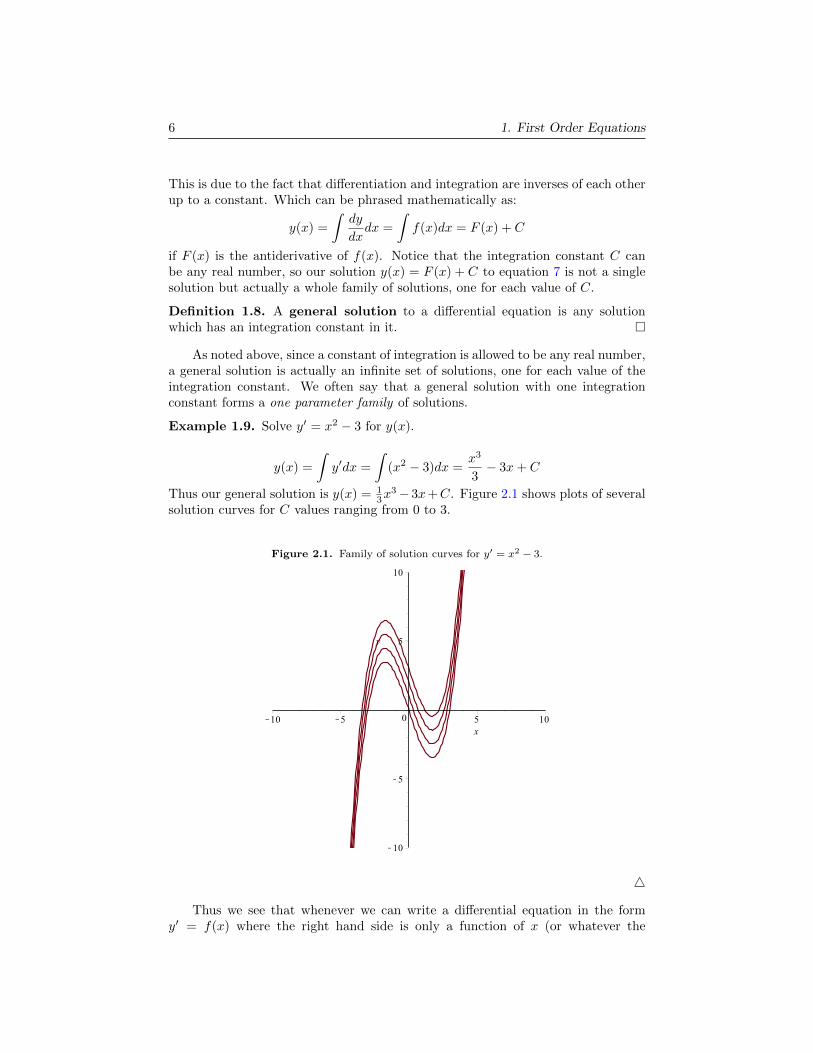
Example 1.9. Solve y′ = x2 − 3 for y(x).
y(x) =
∫y′dx =
∫(x2 − 3)dx =
x3
3− 3x+ C
Thus our general solution is y(x) = 13x
3− 3x+C. Figure 2.1 shows plots of severalsolution curves for C values ranging from 0 to 3.
Figure 2.1. Family of solution curves for y′ = x2 − 3.
4
Thus we see that whenever we can write a differential equation in the formy′ = f(x) where the right hand side is only a function of x (or whatever the

2. Integrals as General and Particular Solutions 7
independent variable is, e.g. t) and does not involve y (or whatever the dependentvariable is), then we can solve the equation merely by integrating. This is veryuseful.
2.1. Initial Value Problems (IVPs) and Particular Solutions.
Definition 1.10. An initial value problem or IVP is a differential equation anda specific point which our solution curve must pass through. It is usually written:
(8) y′ = f(x, y) y(a) = b.
Differential equations had their genesis in solving problems of motion, wherethe indpendent variable is time, t, hence the use of the word “initial”, to conveythe notion of a starting point in time.
Solving an IVP is a two step process. First you must find the general solution.Second you use the initial value y(a) = b to select one particular solution out of thewhole family or set of solutions. Thus a particular solution is a single function whichsatisfies both the governing differential equation and passes through the initial valuea.k.a. initial condition.
Definition 1.11. A particular solution is a solution to an IVP.
Example 1.12. Solve the IVP: y′ = 3x− 2, y(2) = 5.
y(x) =
∫(3x− 2) dx
y(x) =3
2x2 − 2x+ C
y(0) =3
222 − 2 · 2 + C = 5 =⇒ C = 3
y(x) =3
2x2 − 2x+ 3
4
2.2. Acceleration, Velocity, Position. The method of integration extends tohigh order equations. For example, when confronted with a differential equation ofthe form:
(9)d2y
dx2= f(x),
8 1. First Order Equations
we simply integrate twice to solve for y(x), gaining two integration constants alongthe way.
y(x) =
∫dy
dxdx
=
∫ (∫d2y
dx2dx
)dx
=
∫ (∫f(x)dx
)dx
=
∫(F (x) + C1)dx
= G(x) + C1x+ C2
Where we are assuming G′′(x) = F ′(x) = f(x).
Acceleration is the time derivative of velocity (a(t) = v′(t)), and velocity isthe time derivative of position (v(t) = x′(t)). Thus acceleration a(t) is the secondderivative of position x(t) with respect to time, or a(t) = x′′(t).
If we let x(t) denote the position of a body, and we assume that the accelerationthat the body experiences is constant with value a, then in the language of maththis is written as:
(10) x′′(t) = a
The right hand side of this is just the constant function f(t) = a, so thisequation conforms to the form of equation 7. However the function name is xinstead of y and the independent variable is t instead of x, but no matter, they arejust names. To solve for x(t) we must integrate twice with respect to t, time.
(11) v(t) = x′(t) =
∫x′′(t)dt =
∫adt = at+ v0
Here we’ve named our integrtion constant v0 because it must match the initialvelocity, i.e. the velocity of the body at time t = 0. Now we integrate again.
(12) x(t) =
∫v(t)dt =
∫(at+ v0)dt =
1
2at2 + v0t+ x0
Again, we have named the integration constant x0 because it must match theinitial position of the body, i.e. the position of the body at time t = 0.
Example 1.13. Suppose we wish to know how long it will take an object to fallfrom a height of 500 feet down to the ground, and we want to know its velocitywhen it hits the ground. We know from Physics that near the surface of the Earththe acceleration due to gravity is roughly constant with a value of 32 feet per secondper second (f/s2).
Let x(t) represent the vertical position of the object with x = 0 correspondingto the ground and x(0) = x0 = 500. Since up is the positive direction and since the

3. Slope Fields and Solution Curves 9
acceleration of the body is down towards the earth a = −32. Although the problemsays nothing about an initial velocity it is safe to assume that v0 = 0.
x(t) =1
2at2 + v0t+ x0
x(t) =1
2(−32)t2 + 0 · t+ 500
x(t) = −16t2 + 500
We wish to know the time when the object will hit the ground so we wish tosolve the following equation for t:
0 = −16t2 + 500
t2 =500
16
t = ±√
500
16
t = ±5
2
√5
t ≈ ±5.59
So we find that it will take approximately 5.59 seconds to hit the earth. Wecan use this knowledge and equation 11 to compute its velocity at the moment ofimpact.
v(t) = at+ v0
v(t) = −32t
v(5.59) = −32 · 5.59
v(5.59) = −178.88 ft/s
v(5.59) ≈ −122 mi/hr.
4
3. Slope Fields and Solution Curves
In section 1 we noticed that there are some similarities between solving polynomialequations and solving differential equations. Specifically, we noted that it is veryeasy to verify whether a function is a solution to a differential equation simply byplugging it into the equation and checking that the resulting statement is true.This is exactly analogous to checking whether a real number is a solution to apolynomial equation. Here we will explore another similarity. You are certainlyfamiliar with using the quadratic formula for solving quadratic equations, i.e. degreetwo polynomial equations. But you may not know that there are similar formulasfor solving third degree and even fourth degree polynomial equations. Interestingly,it was proved early in the nineteenth century that there is no general formula similarto the quadratic formula which will tell us the roots of all fifth and higher degree

10 1. First Order Equations
polynomial equations in terms of the coefficients. Put simply, we don’t have aformulaic way of solving all polynomial equations. We do have numerical techniques(e.g. Newton’s Method) of approximating the roots which work very well, but thesedo not reveal the exact value.
As you might suspect, since differential equations are generally more compli-cated than polynomial equations the situation is even worse. No procedure exists bywhich a general differential equation can be solved explicitly. Thus, we are forced touse ad hoc methods which work on certain classes of differential equations. There-fore any study of differential equations necessarily requires one to learn various waysto classify equations based upon which method(s) will solve the equation. This isunfortunate.
3.1. Slope Fields and Graphing Approximate Solutions. Luckily, in the caseof first order equations a simple graphical method exists by which we may estimatesolutions by constraints on their graphs. This method of approximate solution usesa special plot called a slope field. Specifically, if we can write a differential equationin the form:
(13)dy
dx= f(x, y)
then we can approximate solutions via the slope field plot. So how does one con-struct such a plot?
The answer lies in noticing that the right hand side of equation 13 is a functionof points in the xy plane which result in the left hand side which is exactly the slopeof y(x), the solution function we seek! If we know the slope of a function at everypoint on the x–axis, then we can graphically reconstruct the solution function y(x).
Creating a slope field plot is normally done via software on a computer. Thebasic algorithm that a computer employs to do this is essentially the following:
(1) Divide the xy plane evenly into a grid of squares.
(2) For each point (xi, yi) in the grid do the following:(a) compute the slope, dy/dx = f(xi, yi).(b) Draw a small bar centered on the point (xi, yi) with slope computed
above. (Each bar should be of equal length and short enough so thatthey do not overlap.)
Let’s use Maple to create a slope field plot for the differential equation
(14) y′ =y
x2 + 1.
with(DEtools):
DE := y’(x) = y(x)/(x^2+1)
dfieldplot(DE, y(x), x=-4..4, y=-4..4, arrows=line)
Maple Listing 1. Slope field plot example. See figure 3.1.
Because any solution curve must be tangent to the bars in the slope field plot,it is fairly easy for your eye to detect possible routes that a solution curve could

3. Slope Fields and Solution Curves 11
Figure 3.1. Slope field plot for y′ = yx2+1
.
take. One can immediately gain a feel for the qualitative behavior of a solutionwhich is often more valuable than a quantitative solution when modeling.
3.2. Creating Slope Field Plots By Hand. The simple algorithm given aboveis fine for a computer program, but is very hard for a human to use in practice.However there is a simpler algorithm which can be done by hand with pencil andgraph paper. The main idea is to find the isoclines in the slopefield, and plotregularly spaced, identical slope bars over the entire length of the isocline.
Definition 1.14. An isocline is a line or curve decorated by regularly spaced shortbars of constant slope.
Example 1.15. Suppose we wish to create a slope–field plot for the differentialequation
dy
dx= x− y = f(x, y).
The method involves two steps. First, we create a table. Each row in thetable corresponds to one isocline. Second, for each row in the table we graph thecorresponding isocline and decorate it with regularly spaced bars, all of which haveequal slope. The slope corresponds to the value in the first column of the table.
Table 1 contains the data for seven isoclines, one for each integer slope valuefrom −3, . . . , 3. We must graph each equation of a line from the third column, anddecorate it with regularly spaced bars where the slope comes from the first column.
Figure 3.2. Isocline slope–field plot for y′ = x− y.

12 1. First Order Equations
m m= f(x, y) y = h(x)
-3 −3 = x− y y = x+ 3-2 −2 = x− y y = x+ 2-1 −1 = x− y y = x+ 10 0 = x− y y = x1 1 = x− y y = x− 12 2 = x− y y = x− 23 3 = x− y y = x− 3
Table 1. Isocline method.
4
3.3. Existence and Uniqueness Theorem. It would be useful to have a simpletest that tells us when a differential equation actually has a solution. We needto be careful here though, because recall that a general solution to a differentialequation is actually an infinite family of solution functions, one for each value ofthe integration constant. We need to be more specific. What we should really askis, “Does my IVP have a solution?” Recall that an IVP (Initial Value Problem) isa differential equation and an initial value,
(8) y′ = f(x, y) y(a) = b.
If a particular solution exists, then our follow up question should be, “Is my partic-ular solution unique?”. The following theorem gives a test that can be performedto answer both questions.
Theorem 1.16 (Existence and Uniqueness). Consider the IVP
dy
dx= f(x, y) y(a) = b
(1) Existence If f(x, y) is continuous on some rectangle R in the xy–planewhich contains the point (a, b), then there exists a solution to the IVP onsome open interval I containing the point a.
(2) Uniqueness If in addition to the conditions in (1), ∂∂yf(x, y) is contin-
uous on R, then the solution to the IVP is unique in I.
Example 1.17. Consider the IVP: y′ = 3√y y(0) = 0. Use theorem 1.16 to
determine (1) whether or not a solution to the IVP exists, and (2) if one does,whether it is unique.
(1) The cube root function is defined for all real numbers, and is continuouseverywhere thus a solution to the IVP exists.

4. Separable Equations and Applications 13
(2) f(x, y) = 3√y = y
13
∂f
∂y=
1
3y−
23
=1
3 3√y2
which is discontinuous at (0, 0), thus the solution is not unique.
4
4. Separable Equations and Applications
In the previous section we explored a method of approximately solving a large classof first order equations of the form dy
dx = f(x, y), where the right hand side is anyfunction of both the independent variable x and the dependent variable y. Thegraphical method of creating a slope field plot is useful, but not ideal because itdoes not yield an exact solution function.
Luckily, a large subclass (subset) of these equations, the so–called separableequations can be solved exactly. Essentially an equation is separable if the righthand side can be factored into a product of two functions, one a function of theindependent variable, and the other a function of the dependent variable.
Definition 1.18. A separable equation is any differential equation that can bewritten in the form:
(15)dy
dx= f(x)g(y).
Example 1.19. Determine whether the following equations are separable or not.
(1)dy
dx= 3x2y − 5xy
(2)dy
dx=
x− 4
y2 + y + 1
(3)dy
dx=√xy
(4)dy
dx= y2
(5)dy
dx= 3y − x
(6)dy
dx= sin(x+ y) + sin(x− y)
(7)dy
dx= exy
(8)dy
dx= ex+y
Solutions:
(1) separable: 3x2y − 5xy = (3x2 − 5x)y

14 1. First Order Equations
(2) separable:x− 4
y2 + y + 1= (x− 4)
(1
y2 + y + 1
)(3) separable:
√xy =
√x√y
(4) separable: y2 = y2 · 1(5) not separable
(6) separable: sin(x+ y) + sin(x− y) = 2 sin(x) cos(y)
(7) not separable
(8) separable: ex+y = ex · ey
4
Before explaining and justifying the method of separation of variables formally,it is helpful to see an example of how it works. A good way to remember thismethod is to remember that it allows us to treat derivatives written using theLeibniz notation as if they were actual fractions.
Example 1.20. Solve the initial value problem:
dy
dx= −kxy, y(0) = 4,
assuming k is a positive constant.
dy
y= −kx dx∫
dy
y= −k
∫x dx
ln |y| = −kx2
2+ C
eln|y| = e(−k x2
2 +C)
|y| = e(− k2 x
2) · eC let C0 = eC
y = C0e(− k
2 x2)
Now plug in x = 0 and set y = 4 to solve for our parameter C0.
4 = C0e0 = C0 =⇒ y(x) = 4e−
k2 x
2
4
There are several steps in the above solution which should raise an eyebrow.First, how can you pretend that the derivative dy/dx is a fraction when clearly itis just a symbol which represents a function? Second, why are we able to integratewith respect to x on the right hand side, but with respect to y which is a function of xon the left hand side? The rest of the solution just involves algebraic manipulationsand is fine.
The answer to both questions above is that what we did is simply “shorthand”for a more detailed, fully correct solution. Let’s start over and solve equation 15.

4. Separable Equations and Applications 15
dy
dx= f(x)g(y)
1
g(y)
dy
dx= f(x)
So far, so good, all we have to watch out for is when g(y) = 0, but that justmeans that our solutions y(x) might not be defined for the whole real line. Next,let’s integrate both sides of the equation with respect to x, and we’ll rewrite y asy(x) to remind us that it is a function of x.∫ (
1
g(y(x))
dy
dx
)dx =
∫f(x) dx
Now, to help us integrate the left hand side, we will make a u–substitution.
u = y(x)
du =dy
dxdx.
∫1
g(u)du =
∫f(x) dx
This equation matches up with the second line in the example above. The“shorthand” technique used in the example skips the step of making the u–substitution.
If we can integrate both sides, then on the left hand side we will have somefunction of u = y(x), which we can hopefully solve for y(x). However, even if wecannot solve for y(x) explicitly, we will still have an implicit solution which can beuseful.
Now, let’s use the above technique of separation of variables to solve the Pop-ulation model from section 1.
Example 1.21. Find the general solution to the population model:
(5)dP
dt= kP.
dP
P= kdt∫
dP
P=
∫k dt
ln |P | = kt+ C
eln|P | = ekt+C
eln|P | = ekt · eC , let P0 = eC
P (t) = P0ekt(16)
4
16 1. First Order Equations
The separation of variables solution technique is important because it allowsus to solve several nonlinear equations. Let’s use the technique to solve equation 6which is the first order, nonlinear differential equation we examined in section 1.
Example 1.22. Solve y′ = y2.
dy
dx= y2∫
dy
y2=
∫dx∫
y−2dy =
∫dx
−y−1 = x+ C
−1
y= x+ C
1
y= C − x absorb negative sign into C
y(x) =1
C − x4
4.1. Radioactive Decay. Most of the carbon in the world is of the isotopecarbon–12, (12
6C), but there are small amounts of carbon–14, (146C) continuously
being created in the upper atmosphere as a result of cosmic rays (neutrons in thiscase) colliding with nitrogen.
10n + 14
7N→ 146C + 1
1p
The resulting 146C is radioactive and will eventually beta decay to 14
7N, an electronand an anti–neutrino:
146C→ 14
7N + e− + νe
The half–life of 146C is 5732 years. This is the time it takes for half of the 14
6C ina sample to decay to 14
7N. The half–life is determined experimentally. From thisknowledge we can solve for the constant of proportionality k:
1
2P0 = P0e
k·5732
1
2= ek·5732
ln
(1
2
)= 5732k
k =ln(1)− ln(2)
5732
k =− ln(2)
5732k ≈ −0.00012092589

4. Separable Equations and Applications 17
The fact that k is negative is to be expected, because we are expecting thepopulation of carbon–14 atoms to diminish as time goes on since we are modelingexponential decay. Let us now see how we can use our new knowledge to reliablydate ancient artifacts.
All living things contain trace amounts of carbon–14. The proportion of carbon–14 to carbon–12 in an organism is equal to the proportion in the atmosphere. Thisis because although carbon atoms in the organism continually decay, new radioac-tive carbon–14 atoms are taken in through respiration or consumption. That is tosay that a living organism whether it be a plant or animal continually replenishesits supply of carbon–14. However, once it dies the process stops.
If we assume that the amount of carbon–14 in the atmosphere has remainedconstant for the past several thousand years, then we can use our knowledge of dif-ferential equations to carbon date ancient artifacts that contain once living materialsuch as wood.
Example 1.23 (Carbon Dating). The logs of an old fort contain only 92% of thecarbon–14 that modern day logs of the same type of wood contain. Assuming thatthe fort was built at about the same time as the logs were cut down, how old is thefort?
Let’s assume that the decrease in the population of carbon–14 atoms is governedby the population equation dy/dt = ky, where y represents the number of carbon–14atoms. From previous work, we know that solution to this equation is y(t) = y0e
kt,where y0 is the initial amount of carbon–14. We know that currently the woodcontains 92% of the carbon–14 that it would have had upon being cut down, thuswe can solve:
0.92y0 = y0ekt
ln(0.92) = kt
t =ln(0.92)
k
t =5732 ln(0.92)
− ln(2)
t ≈ 778 years
4
Figure 4.1. Cell in saltbath
4.2. Diffusion. Another extremely important separableequation comes about from modeling diffusion. Diffusion isthe spreading of something from a concentrated state to aless concentrated state.
We will model the diffusion of salt across a semi–permeable membrane such as a cell wall. Imagine a cell,which contains a salt solution that is immersed in a bathof saline solution. If the salt concentration inside the cell ishigher than outside the cell, then salt will on average, mostly

18 1. First Order Equations
flow out of the cell, and vice versa. Let’s assume that the rate of change of salt con-centration in the cell is proportional to the difference between the concentrationsoutside and inside the cell. Also, let’s assume that the surrounding bath is so muchlarger in volume than the cell, that its concentration remains essentially constantbecause the outflow from the cell is miniscule. We must translate these ideas intoa model. If we let y(t) represent the salt concentration inside the cell, and A theconstant concentration of the surrounding bath, then we get the diffusion equation:
(17)dy
dt= k(A− y)
Again, k is a constant of proportionality with units, 1/time, and we assume k > 0.This is a separable equation, so we know how to solve it.
∫dy
A− y=
∫k dt u = A− y, −du = dy
−∫du
u=
∫k dt
− ln |A− y| = kt+ C
|A− y| = e−kt−C let C0 = e−C
|A− y| = C0e−kt
A− y =
C0e
−kt A > y
−C0e−kt A < y
y = A−
C0e
−kt A > y
−C0e−kt A < y
Thus we get two solutions depending on which concentration is initially higher.
y(t) = A− C0e−kt A > y(18)
y(t) = A+ C0e−kt A < y(19)
Actually, there is a third rather uninteresting solution which occurs when A =y, but then the right hand side of equation 17 is simply 0, which forces y(t) = A,the constant solution. A remark is in order here. Rather than memorizing thesolution, it is far better to become familar with the steps of the solution.
Example 1.24. Suppose a cell with a salt concentration of 5% is immersed in abath of 15% salt solution. If the concentration in the cell doubles to 10% in 10minutes, how long will it take for the salt concentration in the cell to reach 14%?
We wish to solve the IVP:
dy
dt= k(.15− y) y(0) = .05,
along with the extra information y(10) = .10.

4. Separable Equations and Applications 19
∫dy
.15− y=
∫k dt u = .15− y, −du = dy
−∫du
u=
∫k dt
− ln |.15− y| = kt+ C
|.15− y| = e−kt−C
.15− y = C0e−kt
y = .15− C0e−kt
.05 = .15− C0e0 ⇒ C0 = .10
Now we can use the second condition, (point on the solution curve), to deter-mine k:
y(t) = .15− .10e−kt
.10 = .15− .10e−k·10
e−k·10 =.15− .10
.10
−k · 10 = ln
(1
2
)k =
ln(2)− ln(1)
10
k =ln(2)
10
Figure 4.2 graphs a couple of solution curves, for a few different starting cellconcentrations. Notice that in the limit, as time goes to infinity all cells placed inthis salt bath will approach a concentration of 15%. In other words, all cells willeventually come to equilibrium with their environment.
with(DEtools)
DE := y’(t) = k*(A-y(t))
A := .15
k := ln(2)/10
IVS := [y(0)=.25, y(0)=.15, y(0)=.05] # Initial values array
DEplot(DE, y(t), t=0..60, IVS, y=0..0.3, linecolor=navy)
Maple Listing 2. Diffusion example. See figure 4.2.

20 1. First Order Equations
Figure 4.2. Three solution curves for example 1.24, showing the change insalt concentration due to diffusion.
Finally, we wish to find the time at which the salt concentration of the cell willbe exactly 14%. To find this time, we solve the following equation for t:
.14 = .15− .10e−kt
e−kt =.15− .14
.10= .1
−kt = ln
(1
10
)−kt = ln(1)− ln(10)
−kt = − ln(10)
t =ln(10)
k
t =10 ln(10)
ln(2)
t ≈ 33.22 minutes
4
5. Linear First–Order Equations
5.1. Linear vs. Nonlinear Redux. In section 1 we defined a differential equa-tion to be linear if all of its solutions satisfied summability and scalability.
A first–order, linear differential equation is any differential equation which canbe written in the following form:
(20) a(x)y′ + b(x)y = c(x).

5. Linear First–Order Equations 21
If we think of y′ and y as variables, then this equation is reminiscent of linearequations from algebra, except that the coefficients are now allowed to be func-tions of the independent variable x, instead of real numbers. Of course, y and y′
are functions, not variables, but the analogy is useful. Notice that the coefficientfunctions are strictly forbidden from being functions of y or any of its derivatives.
The above definition of linear extends to higher–order equations. For example,a fourth order, linear differential equation can be written in the form:
(21) a4(x)y(4) + a3(x)y′′′ + a2(x)y′′ + a1(x)y′ + a0(x)y = f(x)
Definition 1.25. In general, an n–th order, linear differential equation is anyequation which can be written in the form:
(22) an(x)y(n) + an−1(x)y(n−1) + · · ·+ a1(x)y′ + a0(x)y = f(x).
This is not just a working definition. It is the definition that we will continueto use throughout the text. Notice that this definition is very different from theprevious definition in section 1. That definition suffered from the defect that it wasimpossible to positively determine whether an equation was linear. We could onlyuse it to determine when a differential equation is nonlinear. The above definitionis totally different. You can use the above definition to tell on sight (with practice)whether or not a given differential equation is linear. Also notice that it suffers frombeing a poor tool for determining whether a given differential equation is nonlinear.This is because, you don’t know if perhaps your are just not being clever enoughto write the equation in the form of the definition.
These notes focus on solving linear equations, however recall from section 4that we can solve nonlinear, first–order equations when they are separable. How-ever, in general, solving higher order, nonlinear differential equations is much moredifficult. However, not all is lost. A Norwegian mathematician named Sophus Lie(prononunced “lee”) discovered that if a differential equation possesses a type oftransfomational symmetry, then that symmetry can be used to find solutions of theequation. His work led a German mathematician, Hermann Weyl, to extend Lie’sideas and today Weyl’s work forms the foundations of much of modern QuantumMechanics. Lie’s symmetry methods are beyond the scope of this book, but if youare a Physics student, you should definitely look into them after completing thiscourse.
5.2. The Integrating Factor Method. Good news. We can solve any firstorder, linear differential equation! The caveat here is that the method involvesintegration, so a solution function might have to be defined in terms of an integral,that is, it might be an accumulation function.
The first step in this method is to divide both sides of equation 20 by thecoefficient function of y′, i.e. a(x).
a(x)y′ + b(x)y = c(x) =⇒ y′ +b(x)
a(x)y =
c(x)
a(x)
22 1. First Order Equations
We will rename b(x)/a(x) to p(x) and c(x)/a(x) to q(x) and rewrite this equa-tion in what we will call standard form for a first order, linear equation.
(23) y′ + p(x)y = q(x)
The reason for using p(x) and q(x) is simply because they are easier to writethan b(x)/a(x) and c(x)/a(x). The heart of the method is what follows. If theleft hand side of equation 23 were the derivative of some expression, then we couldperhaps get rid of the prime on y′ by integrating both sides and then algebraicallysolve for y(x). Notice that the left hand side of equation 23 almost resembles theresult of differentiating the product of two functions. Recall the product rule:
d
dx[uv] = u′v + uv′.
Perhaps we can multiply both sides of equation 23 by something that will makethe left hand side into an expression which is the derivative of a product of twofunctions. Remember, however, that we must multiply both sides of the equationby the same factor or else we will be solving an entirely different equation. Let’scall this factor ρ(x) because the Greek letter “rho” resembles the Latin letter “p”,and we will see that p(x) must be related to ρ(x). That is we want:
(24)d
dx[yρ] = y′ρ+ ypρ
By comparing with the product rule, we find that if ρ′ = pρ, then the expressiony′ρ + ypρ′ will indeed be the derivative of the product yρ. Notice that we havereduced the problem down to solving a first order, separable equation that weknow how to solve.
(25) ρ′ = p(x)ρ =⇒ ρ = e∫p(x)dx
Upon multiplying both sides of equation 23 by the integrating factor ρ fromequation 25, we get:
(ye∫p(x)dx)′ = q(x)e
∫p(x)dx∫
(ye∫p(x)dx)′dx =
∫q(x)e
∫p(x)dxdx
ye∫p(x)dx =
∫q(x)e
∫p(x)dxdx
y = e−∫p(x)dx
∫q(x)e
∫p(x)dxdx
You should not try to memorize the formula above. Instead remember thefollowing steps:
(1) Put the first order linear equation in standard form.
(2) Calculate ρ(x) = e∫p(x)dx.
(3) Multiply both sides of the equation by ρ(x).
(4) Integrate both sides.
5. Linear First–Order Equations 23
(5) Solve for y(x).
Example 1.26. Solve xy′ − y = x3 for y(x).
(1) y′ − 1
xy = x2
(2) ρ(x) = e−∫
dxx = e− ln|x| = eln(|x|−1) =
1
|x|=
1
xx > 0
(3) y′1
x− y 1
x2= x2 1
x
(4)∫ (
y1
x
)′dx =
∫xdx =⇒ y
1
x=
1
2x2 + C
(5) y =1
2x3 + Cx x > 0
4
An important fact to notice is that we ignore the constant of integration whencomputing the integrating factor ρ. This is because the constant of integration ispart of the exponent of e. Assume P (x) is the antiderivative of p(x), then
ρ = e∫p(x)dx = e(P (x)+C) = eC · eP (x) = C1e
P (x).
Since we multiply both sides of the equation by the integrating factor, the C1s cancelout.
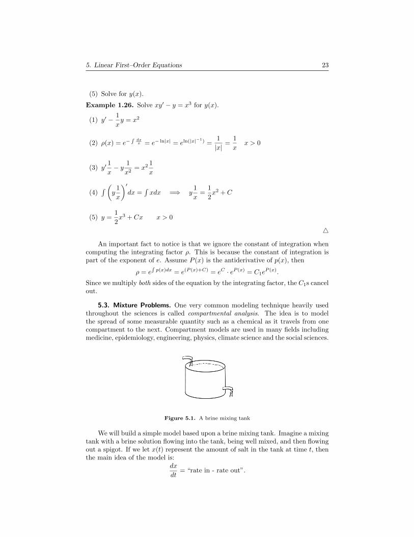
5.3. Mixture Problems. One very common modeling technique heavily usedthroughout the sciences is called compartmental analysis. The idea is to modelthe spread of some measurable quantity such as a chemical as it travels from onecompartment to the next. Compartment models are used in many fields includingmedicine, epidemiology, engineering, physics, climate science and the social sciences.
Figure 5.1. A brine mixing tank
We will build a simple model based upon a brine mixing tank. Imagine a mixingtank with a brine solution flowing into the tank, being well mixed, and then flowingout a spigot. If we let x(t) represent the amount of salt in the tank at time t, thenthe main idea of the model is:
dx
dt= “rate in - rate out”.

24 1. First Order Equations
We will use the following names/symbols for the different quantities in the model:
Symbol Interpretation
x(t) = amount of salt in the tank (lbs)ci(t) = concentration of incoming solution (lbs/gal)fi(t) = flow rate of incoming solution (gal/min)co(t) = concentration of outgoing solution (lbs/gal)fo(t) = flow rate of outgoing solution (gal/min)v(t) = amount of brine in the tank (gal)
Notice that if you multiply a concentration by a flow rate, then the units willbe lbs/min which exactly match the units of the derivative dx/dt, hence our modelis:
(26)dx
dt= ci(t)fi(t)− co(t)fo(t)
Often, ci, fi and fo will be fixed quantities, but co(t) depends upon the amountof salt in the tank at time t, and the volume of brine in the tank at that time. If weassume that the incoming salt solution and the solution in the tank are perfectlymixed, then:
(27) co(t) =x(t)
v(t).
Often the flow rate in, fi, and the flow rate out, fo, will be equal. When thisis the case, the volume of the tank will remain constant. However if the two flowrates do not match, then v(t) = [fi(t)− fo(t)]t+ v0, where v0 is the initial volumeof the tank. Now we can rewrite equation 26, in the same form as the standardfirst order linear equation.
(28)dx
dt+fo(t)
v(t)x = ci(t)fi(t)
Example 1.27 (Brine Tank). A tank initially contains 200 gallons of brine, holding50 lbs of salt. Salt water (brine) containing 2 lbs of salt per gallon flows into thetank at a constant rate of 4 gal/min. The mixture is kept uniform by constantstirring, and the mixture flows out at a rate of 4 gal/min. Find the amount of saltin the tank after 40 minutes.
dx
dt= cifi − cofo
dx
dt=
(2 lb
gal
)(4 gal
min
)−(
x lb
200 gal
)(4 gal
min
)dx
dt= 8− 1
50x
dx
dt+
1
50x = 8
5. Linear First–Order Equations 25
This equation can be solved via the integrating factor technique.
ρ(t) = e∫
150 dt = et/50
x′et/50 +1
50xet/50 = 8et/50
d
dt
[xet/50
]= 8et/50∫
d
dt
[xet/50
]dt = 8
∫et/50 dt
xet/50 = 8 · 50et/50 + C
x(t) = e−t/50[400et/50 + C]
x(t) = 400 + Ce−t/50
Next we apply the initial condition x(0) = 50:
50 = 400 + Ce0 =⇒ C = −350
Finally, we compute x(40).
x(t) = 400− 350e−t/50
x(40) = 400− 350e−40/50
x(40) ≈ 242.7 lbs
Notice that limt→∞ x(t) = 400, which is exactly how much salt would be in a200 gallon tank filled with brine at the incoming concentration of 2 lbs/gal. 4
In the previous example the inflow rate, fi and the outflow rate, fo were equal.This results in a convenient situation where the volume in the tank remains con-stant. However, this does not have to be the case. If fi 6= fo, then we need to finda valid expression for v(t).
Example 1.28. Suppose we again have a 200 gallon tank that is initially filledwith 50 gallons of pure water. If water flows in at a rate of 5 gal/min and flows outat a rate of 3 gal/min, when will the tank be full?
The rate at which the volume of fluid in the tank changes depends on twofactors, the initial volume of the tank, and the difference in flow rates.
v(t) = v0 + [fi(t)− fo(t)]t
In this example, we have:
v(t) = 50 + [5− 3]t
v(t) = 50 + 2t.
The tank will be completely full when v(t) = 200, and this will occur when t =75. 4
26 1. First Order Equations
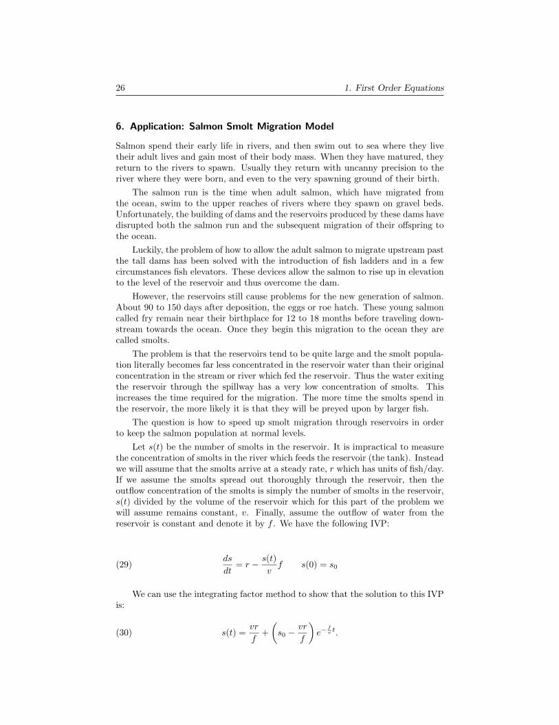
6. Application: Salmon Smolt Migration Model
Salmon spend their early life in rivers, and then swim out to sea where they livetheir adult lives and gain most of their body mass. When they have matured, theyreturn to the rivers to spawn. Usually they return with uncanny precision to theriver where they were born, and even to the very spawning ground of their birth.
The salmon run is the time when adult salmon, which have migrated fromthe ocean, swim to the upper reaches of rivers where they spawn on gravel beds.Unfortunately, the building of dams and the reservoirs produced by these dams havedisrupted both the salmon run and the subsequent migration of their offspring tothe ocean.
Luckily, the problem of how to allow the adult salmon to migrate upstream pastthe tall dams has been solved with the introduction of fish ladders and in a fewcircumstances fish elevators. These devices allow the salmon to rise up in elevationto the level of the reservoir and thus overcome the dam.
However, the reservoirs still cause problems for the new generation of salmon.About 90 to 150 days after deposition, the eggs or roe hatch. These young salmoncalled fry remain near their birthplace for 12 to 18 months before traveling down-stream towards the ocean. Once they begin this migration to the ocean they arecalled smolts.
The problem is that the reservoirs tend to be quite large and the smolt popula-tion literally becomes far less concentrated in the reservoir water than their originalconcentration in the stream or river which fed the reservoir. Thus the water exitingthe reservoir through the spillway has a very low concentration of smolts. Thisincreases the time required for the migration. The more time the smolts spend inthe reservoir, the more likely it is that they will be preyed upon by larger fish.
The question is how to speed up smolt migration through reservoirs in orderto keep the salmon population at normal levels.
Let s(t) be the number of smolts in the reservoir. It is impractical to measurethe concentration of smolts in the river which feeds the reservoir (the tank). Insteadwe will assume that the smolts arrive at a steady rate, r which has units of fish/day.If we assume the smolts spread out thoroughly through the reservoir, then theoutflow concentration of the smolts is simply the number of smolts in the reservoir,s(t) divided by the volume of the reservoir which for this part of the problem wewill assume remains constant, v. Finally, assume the outflow of water from thereservoir is constant and denote it by f . We have the following IVP:
(29)ds
dt= r − s(t)
vf s(0) = s0
We can use the integrating factor method to show that the solution to this IVPis:
(30) s(t) =vr
f+
(s0 −
vr
f
)e−
fv t.
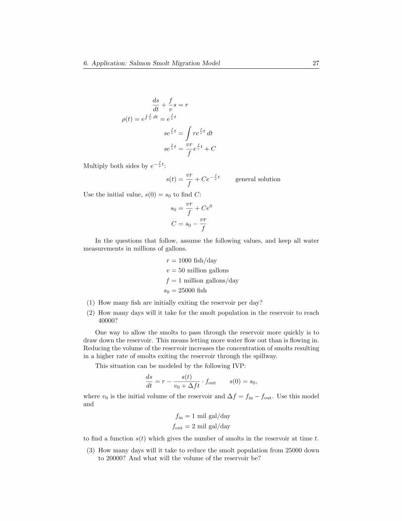
6. Application: Salmon Smolt Migration Model 27
ds
dt+f
vs = r
ρ(t) = e∫ f
v dt = efv t
sefv t =
∫re
fv t dt
sefv t =
vr
fe
fv t + C
Multiply both sides by e−fv t:
s(t) =vr
f+ Ce−
fv t general solution
Use the initial value, s(0) = s0 to find C:
s0 =vr
f+ Ce0
C = s0 −vr
f
In the questions that follow, assume the following values, and keep all watermeasurements in millions of gallons.
r = 1000 fish/day
v = 50 million gallons
f = 1 million gallons/day
s0 = 25000 fish
(1) How many fish are initially exiting the reservoir per day?
(2) How many days will it take for the smolt population in the reservoir to reach40000?
One way to allow the smolts to pass through the reservoir more quickly is todraw down the reservoir. This means letting more water flow out than is flowing in.Reducing the volume of the reservoir increases the concentration of smolts resultingin a higher rate of smolts exiting the reservoir through the spillway.
This situation can be modeled by the following IVP:
ds
dt= r − s(t)
v0 + ∆ft· fout s(0) = s0,
where v0 is the initial volume of the reservoir and ∆f = fin − fout. Use this modeland
fin = 1 mil gal/day
fout = 2 mil gal/day
to find a function s(t) which gives the number of smolts in the reservoir at time t.
(3) How many days will it take to reduce the smolt population from 25000 downto 20000? And what will the volume of the reservoir be?

28 1. First Order Equations
7. Homogeneous Equations
A homogeneous function is a function with multiplicative scaling behaviour. If theinput is multiplied by some factor then the output is multiplied by some power ofthis factor. Symbolically, if we let α be a scalar—any real number, then a functionf(x) is homogeneous if f(αx) = αkf(x) for some positive integer k. For example,f(x) = 3x is homogeneous of degree 1 because
f(αx) = 3(αx) = α3x = αf(x).
In this example k = 1, hence we say f is homogeneous of degree one. A functionwhose graph is a line which does not pass through the origin, such as g(x) = 3x+ 1is not homogeneous because,
g(αx) = 3(αx) + 1 = α(3x) + 1 6= α(3x+ 1) = αg(x).
Definition 1.29. A multivariable function, f(x, y, z) is homogeneous of degree k,if given a real number α the following holds
f(αx, αy, αz) = αkf(x, y, z).
In other words, scaling all of the inputs by the same factor results in the outputbeing scaled by some power of that factor.
Monomials in n variables form homogeneous functions. For example, the mono-mial in three variables: f(x, y, z) = 4x3y5z2 is homogeneous of degree 10 since,
f(αx, αy, αz) = 4(αx)3(αy)5(αz)2 = α10(4x3y5z2) = α10f(x, y, z).
Clearly, the degree of a monomial function is simply the sum of the exponentson each variable. Polynomials formed from monomials of the same degree arehomogeneous functions. For example, the polynomial function
g(x, y) = x3 + 5x2y + 9xy2 + y3
is homogeneous of degree three since, g(αx, αy) = α3g(x, y).
Definition 1.30. A first order differential equation is homogeneous if it can bewritten in the form
(31) a(x, y)dy
dx+ b(x, y) = 0,
where a(x, y) and b(x, y) are homogeneous functions of the same degree.
Suppose both a(x, y) and b(x, y) from equation (31) are of degree k, then wecan rewrite equation (31) in the following manner:
(32)dy
dx= −ZZxk b
(1,y
x
)ZZxk a
(1,y
x
) = F(yx
).
An example will illustrate the rewrite rule demonstrated in equation (32).
7. Homogeneous Equations 29
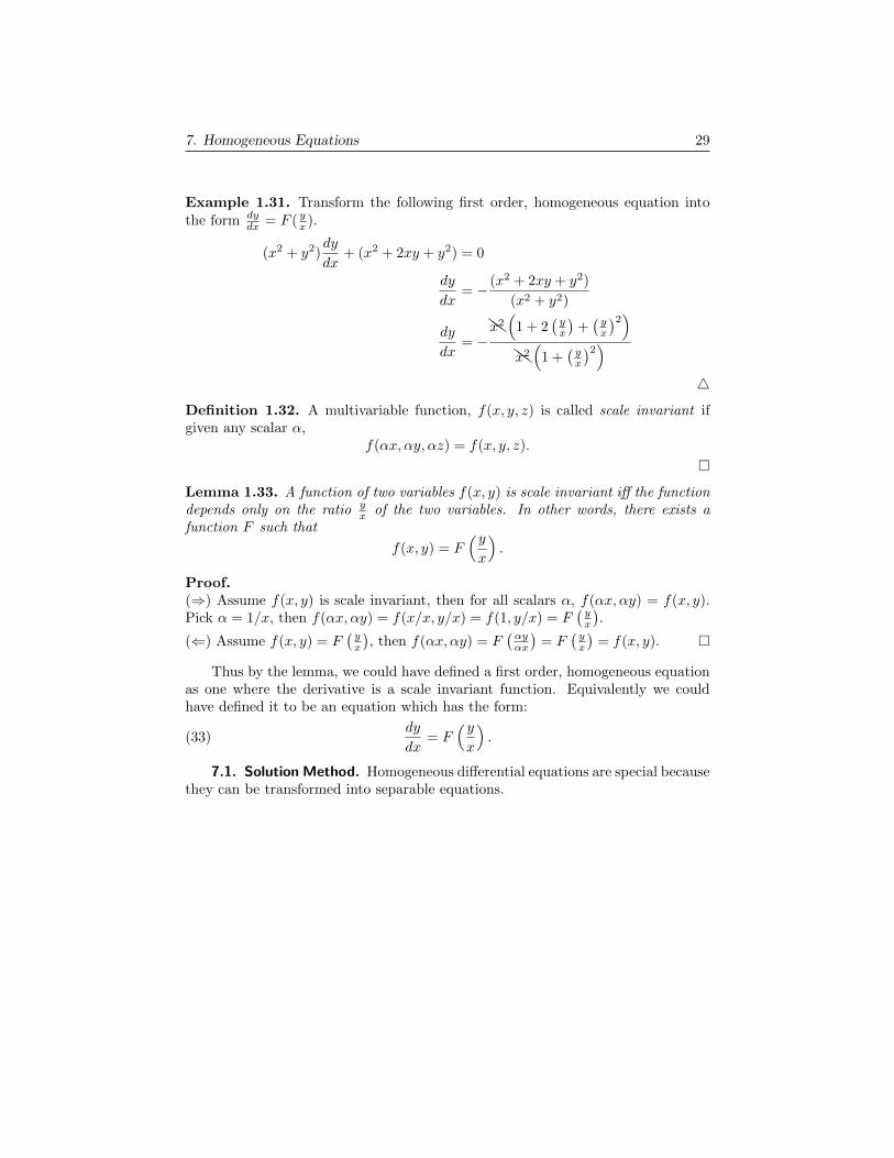
Example 1.31. Transform the following first order, homogeneous equation intothe form dy
dx = F ( yx ).
(x2 + y2)dy
dx+ (x2 + 2xy + y2) = 0
dy
dx= − (x2 + 2xy + y2)
(x2 + y2)
dy
dx= −ZZx2(
1 + 2(yx
)+(yx
)2)ZZx2(
1 +(yx
)2)4
Definition 1.32. A multivariable function, f(x, y, z) is called scale invariant ifgiven any scalar α,
f(αx, αy, αz) = f(x, y, z).
Lemma 1.33. A function of two variables f(x, y) is scale invariant iff the functiondepends only on the ratio y
x of the two variables. In other words, there exists afunction F such that
f(x, y) = F(yx
).
Proof.(⇒) Assume f(x, y) is scale invariant, then for all scalars α, f(αx, αy) = f(x, y).Pick α = 1/x, then f(αx, αy) = f(x/x, y/x) = f(1, y/x) = F
(yx
).
(⇐) Assume f(x, y) = F(yx
), then f(αx, αy) = F
(αyαx
)= F
(yx
)= f(x, y).
Thus by the lemma, we could have defined a first order, homogeneous equationas one where the derivative is a scale invariant function. Equivalently we couldhave defined it to be an equation which has the form:
(33)dy
dx= F
(yx
).
7.1. Solution Method. Homogeneous differential equations are special becausethey can be transformed into separable equations.

Chapter 2
Models and NumericalMethods
1. Population Models
1.1. The Logistic Model. Our earlier population model suffered from the factthat eventually the population would “blow up” and grow at unrealistic rates. Thiswas due to the fact that the solution involved an exponential function. Recall themodel and solution:
dP
dt= kP(5)
P (t) = P0ekt.(16)
Bacteria in a petri dish can’t reproduce forever because they eventually run outof food and space. In our previous population model, the constant of proportionalitywas actually the birth rate minus the death rate: k = β − δ, where k and thereforealso β and δ have units of 1/time.
To make our model more realistic, we need the birth rate to taper off as the pop-ulation reaches a certain number or size. Perhaps the simplest way to accomplishthis is to have it decrease linearly with population size.
β(P ) = β0 − β1P
For this to make sense in the original equation, β0 must have units of 1/time, andβ1 must have units of 1/(population·time). Let’s incorporate this new, decreasingbirth rate into the original population model.
31

32 2. Models and Numerical Methods
dP
dt= [(β0 − β1P )− δ]P
= P [(β0 − δ)− β1P ]
= β1P
[β0 − δβ1
− P]
In order to get a simple, easy to remember equation, let’s let k = β1 and M = β0−δβ1
.
(34)dP
dt= kP (M − P )
Notice that M has units of population. We have specifically written equation 34,in the form at the bottom of the derivation because M has a special meaning, it isthe carrying capacity of the population.
Notice that equation 34 is separable, so we know how to go about solving it.However, before we solve the logistic model, let’s refresh our memory of solvingintegrals via partial fractions, because we will need to use this when solving thelogistic model. Let’s solve a simplified version of the logistic model, with k = 1 andM = 1.
(35)dx
dt= x(1− x)
∫1
x(1− x)dx =
∫dt∫ (
A
x+
B
(1− x)
)dx =
∫dt
A(1− x) +Bx = 1
x = 0 : A(1− 0) +B · 0 = 1⇒ A = 1
x = 1 : A(1− 1) +B · 1 = 1⇒ B = 1∫ (1
x+
1
(1− x)
)dx =
∫dt
ln |x| − ln |1− x| = t+ C0
ln
∣∣∣∣ x
1− x
∣∣∣∣ = t+ C0∣∣∣∣ x
1− x
∣∣∣∣ = et+C0 = C1et
∣∣∣∣ x
1− x
∣∣∣∣ =
x
1− xx
1− x≥ 0 0 ≤ x < 1
x
x− 1
x
1− x< 0 x < 0
⋃x > 1

1. Population Models 33
Let’s solve for x(t) for 0 ≤ x < 1:
x = (1− x)C1et
x+ C1xet = x0e
t
x(1 + C1et) = C1e
t
x =C1e
t
1 + C1et
x(t) =1
1 + Ce−t(36)
When x < 0 or x > 1, then we get:
(37) x(t) =1
1− Ce−t
The last solution occurs when x(t) = 1, because this forces dx/dt = 0.
Figure 1.1 shows some solution curves superimposed on the slope field plot forx′ = x(1−x). Notice that the solution x(t) = 1 seems to “attract” solution curves,but the solution x(t) = 0, “repels” solution curves.
Figure 1.1. Slope field plot and solution curves for x′ = x(1 − x).
Let us now use what we just learned to solve the logistic model, with an initialcondition.
(34)dP
dt= kP (M − P ) P (0) = P0

34 2. Models and Numerical Methods
∫1
P (M − P )dP =
∫k dt∫
1/M
P+
1/M
(M − P )dP =
∫k dt∫
1
P+
1
(M − P )dP =
∫kM dt
ln
∣∣∣∣ P
M − P
∣∣∣∣ = kMt+ C0∣∣∣∣ P
M − P
∣∣∣∣ = C1ekMt
∣∣∣∣ P
M − P
∣∣∣∣ =
P
M − P0 ≤ P < M
P
P −MP < 0
⋃P > M
If we solve for the first case, we find:
P = (M − P )C1ekMt
P + PC1ekMt = MC1e
kMt
P =MC1e
kMt
1 + C1ekMt· e−kMt
e−kMt
P =MC1
e−kMt + C1.(38)
Now we can plug in the initial condition to get a particular solution:
P0 =MC1
1 + C1
P0 + P0C1 = MC1
P0 = MC1 − P0C1
C1 =P0
M − P0
P (t) =M(
P0
M−P0
)e−kMt +
(P0
M−P0
)P (t) =
MP0
P0 + (M − P0)e−kMt.(39)
2. Equilibrium Solutions and Stability
Whenever the right hand side of a first order equation only involves the dependentvariable, then we can quickly determine the qualitative behavior of its solutions.

2. Equilibrium Solutions and Stability 35
For example, if a differential equation has the form:
(40)dy
dx= f(y).
Definition 2.1. When the independent variable does not appear explicitly in adifferential equation, we say that equation is autonomous.
Recall from section 3 how a computer makes a slope field plot. It simply gridsoff the xy–plane and then at each vertex of the grid draws a short bar with slopecorresponding to f(xi, yi), however if the right hand side function is only a functionof the dependent variable, y in this case, then the slope field does not depend onthe independent variable, i.e. location on the x–axis. This means that for anautonomous equation, the slopes which lie on a horizontal line such as y = 2 areall equivalent and thus parallel.
This means that if a solution curve is shifted (translated) left or right alongthe x-axis, then this shifted curve will also be a solution curve, because it willstill fit the slope field. We have established an important property of autonomousequations, namely translation invariance.
2.1. Phase Diagrams. Consider the following autonomous differential equa-tion:
(41) y′ = y(y − 2).
Notice that the two constant functions y(x) = 0, and y(x) = 2 are solutionsto equation 41. In fact any time you have an autonomous equation, any constantfunction which makes the right hand side of the equation zero will be a solution.This is because constant functions have slope zero. Thus as long as this constantvalue of y is a root of the right hand side, then that particular constant functionwill satisfy the equation. Notice that other constant functions such as y(x) = 1and y(x) = 3 are not solutions of equation 41, because y′ = 1(1− 2) = −1 6= 0 andy′ = 3(3− 2) = 1 6= 0 respectively.
Definition 2.2. Given an autonomous first order equation: y′ = f(y), the solutionsof f(y) = 0 are called critical points of the equation.
So the critical points of equation 41 are y = 0 and y = 2.
Definition 2.3. If c is a critical point of the autonomous first order equationy′ = f(y), then y(x) ≡ c is an equilibrium solution of the equation.
So the equilibrium solutions of equation 41, are y(x) = 0 and y(x) = 2. Some-thing in equilibrium, is something that has settled and does not change with time,i.e. is contant.
To create the phase diagram for this function we pick y values surrounding thecritical points to determine whether the slope is positive or negative.
y = −1 : −1(−1− 2) = (−) (−) = +
y = 1 : 1(1− 2) = (+) (−) = −y = 3 : 3(3− 2) = (+) (+) = +

36 2. Models and Numerical Methods
Example 2.4. Create a phase diagram and plot several solution curves by handfor the differential equation: dx/dt = x3 − 7x2 + 10x.
We factor the right hand side to find the critical points and hence equilibriumsolutions.
x3 − 7x2 + 10x = 0
x(x2 − 7x+ 10) = 0
x(x− 2)(x− 5) = 0
The critical points are x = 0, 2, 5, and thus the equilibrium solutions are x(t) =0, x(t) = 2 and x(t) = 5.
Figure 2.1. Phase diagram for y′ = y(y − 2).
Figure 2.2. Phase diagram for x′ = x3 − 7x2 + 10x.
Figure 2.3. Hand drawn solution curves for x′ = x3 − 7x2 + 10x.
2. Equilibrium Solutions and Stability 37
4
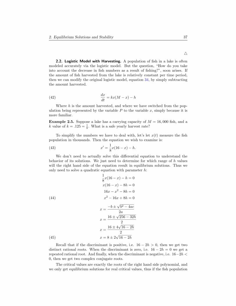
2.2. Logistic Model with Harvesting. A population of fish in a lake is oftenmodeled accurately via the logistic model. But the question, “How do you takeinto account the decrease in fish numbers as a result of fishing?”, soon arises. Ifthe amount of fish harvested from the lake is relatively constant per time period,then we can modify the original logistic model, equation 34, by simply subtractingthe amount harvested.
(42)dx
dt= kx(M − x)− h
Where h is the amount harvested, and where we have switched from the pop-ulation being represented by the variable P to the variable x, simply because it ismore familiar.
Example 2.5. Suppose a lake has a carrying capacity of M = 16, 000 fish, and ak value of k = .125 = 1
8 . What is a safe yearly harvest rate?
To simplify the numbers we have to deal with, let’s let x(t) measure the fishpopulation in thousands. Then the equation we wish to examine is:
(43) x′ =1
8x(16− x)− h.
We don’t need to actually solve this differential equation to understand thebehavior of its solutions. We just need to determine for which range of h valueswill the right hand side of the equation result in equilibrium solutions. Thus weonly need to solve a quadratic equation with parameter h:
1
8x(16− x)− h = 0
x(16− x)− 8h = 0
16x− x2 − 8h = 0
x2 − 16x+ 8h = 0(44)
x =−b±
√b2 − 4ac
2a
x =16±
√256− 32h
2
x =16± 4
√16− 2h
2
x = 8± 2√
16− 2h(45)
Recall that if the discriminant is positive, i.e. 16 − 2h > 0, then we get twodistinct rational roots. When the discriminant is zero, i.e. 16 − 2h = 0 we get arepeated rational root. And finally, when the discriminant is negative, i.e. 16−2h <0, then we get two complex conjugate roots.
The critical values are exactly the roots of the right hand side polynomial, andwe only get equilibrium solutions for real critical values, thus if the fish population
38 2. Models and Numerical Methods
(a) h = 10 (b) h = 8
(c) h = 7.5 (d) h = 6
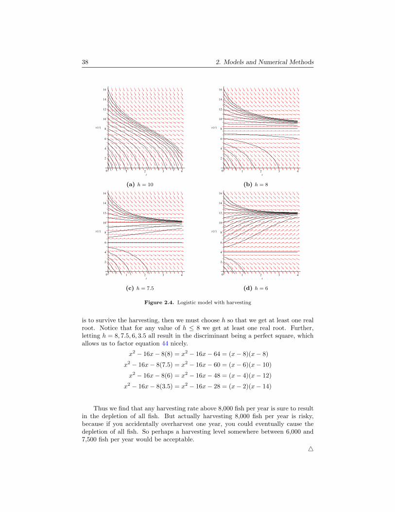
Figure 2.4. Logistic model with harvesting
is to survive the harvesting, then we must choose h so that we get at least one realroot. Notice that for any value of h ≤ 8 we get at least one real root. Further,letting h = 8, 7.5, 6, 3.5 all result in the discriminant being a perfect square, whichallows us to factor equation 44 nicely.
x2 − 16x− 8(8) = x2 − 16x− 64 = (x− 8)(x− 8)
x2 − 16x− 8(7.5) = x2 − 16x− 60 = (x− 6)(x− 10)
x2 − 16x− 8(6) = x2 − 16x− 48 = (x− 4)(x− 12)
x2 − 16x− 8(3.5) = x2 − 16x− 28 = (x− 2)(x− 14)
Thus we find that any harvesting rate above 8,000 fish per year is sure to resultin the depletion of all fish. But actually harvesting 8,000 fish per year is risky,because if you accidentally overharvest one year, you could eventually cause thedepletion of all fish. So perhaps a harvesting level somewhere between 6,000 and7,500 fish per year would be acceptable.
4

3. Acceleration–Velocity Models 39
3. Acceleration–Velocity Models
In section 2 we modeled a falling object, but we ignored the frictional force due towind resistance. Let’s fix that omission.
The force due to wind resistance can be modeled by positing that the force willbe in the opposite direction of motion, but proportional to velocity.
(46) FR = −kv
Recall from physics that Newton’s second law of motion: ΣF = ma = m(dv/dt),relates the sum of the forces acting on a body with its rate of change of momemtum.There are two forces acting on a falling body, one is the pull of gravity, and theother is a buoying force due to wind resistance. If we set up our y–axis with thepositive y direction pointing upward and let zero correspond to ground level, thenFR = −kv = −k(dy/dt). Note that this is an upward force because v is negative,thus the sum of the forces is:
(47) ΣF = FR + FG = −kv −mg.
Hence our governing IVP becomes:
mdv
dt= −kv −mg
dv
dt= − k
mv − g
dv
dt= −ρv − g v(0) = v0(48)
This is a separable, first–order equation. Let’s solve it.
∫1
ρv + gdv = −
∫dt
1
ρln |ρv + g| = −t+ C
ln |ρv + g| = −ρt+ C
eln|ρv+g| = e−ρt+C
|ρv + g| = Ce−ρt
ρv + g =
Ce−ρt ρv + g ≥ 0
−Ce−ρt ρv + g < 0
v(t) =
Ce−ρt − g
ρv ≥ −g
ρ
−Ce−ρt − g
ρv < −g
ρ

40 2. Models and Numerical Methods
Next, we plug in the initial condition v(0) = v0 to get a particular solution.
v0 = C − g
ρ
C = v0 +g
ρ
v(t) =
(v0 + g
ρ
)e−ρt − g
ρv ≥ −g
ρ
−(v0 + g
ρ
)e−ρt − g
ρv < −g
ρ
(49)
Notice that the limit as time goes to infinity of both solutions is the same.
(50) limt→∞
v(t) = limt→∞
±(v0 +
g
ρ
)e−ρt − g
ρ= −g
ρ= −mg
k
This limiting velocity is called terminal velocity. It is the fastest speed that adropped object can achieve. Notice that it is negative because it is a downwardvelocity.
The first solution of equation 49 handles the situation where the body is fallingmore slowly than terminal velocity. The second solution handles the case wherethe body or object is falling faster than terminal velocity, for example a projectileshot downward.
Example 2.6. In example 1.13 we calculated that it would take approximately5.59 seconds for an object to fall 500 feet, but we neglected the effects of windresistance. Compute how long it will take for an object to fall 500 feet if ρ = .16,and compute its final velocity.
Recall that v(t) = dy/dt, and since v(t) is only a function of the independentvariable, t, we can integrate the velocity to find the position as a function of time.Since we are dropping the object from 500 feet, y0 = 500 and v0 = 0.
y(t) =
∫dy
dtdt =
∫v(t) dt
y(t) =
∫ [(v0 +
g
ρ
)e−ρt − g
ρ
]dt
y(t) =
(v0 +
g
ρ
)∫e−ρt dt− g
ρ
∫dt
y(t) =
(v0 +
g
ρ
)(−1
ρ
)e−ρt −
(g
ρ
)t+ C
500 = −(
32
(.16)2
)+ C
C = 500 + 1250
C = 1750
y(t) = −1250e−.16t − 200t+ 1750(51)
As you can see in figure 3.1, when we model the force due to wind resistance itadds almost a full second to the amount of time that it takes for an object to fall

4. Numerical Solutions 41
Figure 3.1. Falling object with and without wind resistance
500 feet. In fact it takes approximately 6.56 seconds to reach the ground. Knowingthis, we can compute the final velocity.
v(6.56) = −1250e−.16(6.56) − 200(6.56) + 1750
= −1250e−.16(6.56) − 200(6.56) + 1750
≈ −130 ft/s
(60 mi/hr
88 ft/s
)≈ −89
mi
hr
Thus it takes almost a full second longer to reach the ground (6.56 s vs. 5.59 s)and will be travelling at approximately -89 miles per hour as opposed to -122 milesper hour.
4
4. Numerical Solutions
In actual real–world applications, more often than not, you won’t be able to findan analytic solution to the general first order IVP.
(13)dy
dx= f(x, y) y(a) = b
In this situation it often makes sense to approximate a solution via simulation.We will look at an algorithm for creating approximate solutions called Euler’sMethod, and named after Leonhard Euler, (pronounced like “oiler”). The algorithm

42 2. Models and Numerical Methods
is easier to explain if the independent variable is time, so let’s rewrite the generalfirst order equation above using time, t as the independent variable:
(13)dy
dt= f(t, y) y(t0) = y0.
The fundamental idea behind Euler’s Method and all numerical/simulationtechniques is discretization. Essentially the idea is to change the independent vari-able time, t, from something that can take on any real number, to a variable thatis only allowed to have values from a discrete, i.e. finite sequence. Each time valueis separated from the next by a fixed period of time, the “tick” of our clock. Thelength of this “tick” depends on how accurately we wish to approximate exactsolutions. Shorter tick lengths will result in more accurate approximations.
Normally a solution function must be continuous, and smooth, a.k.a. differ-entiable. Discretizing time forces us to relax the smoothness requirement. Theapproximate solution curves we create will be continuous, but not smooth. Theywill have small angular corners at each tick of the clock, i.e. at each time in thediscrete sequence of allowed time values.
The goal of the algorithm is to create a sequence of pairs (ti, yi) which whenplotted and connected by straight line segments will approximate exact solutioncurves. The method of generating this sequence is recursive, i.e. computing thenext pair in the sequence will require us to know the values of the previous pair inthe sequence. This recursion is written via two equations:
ti+1 = ti + ∆t
yi+1 = yi + ∆y,
where the subscript i+1 refers to the “next” value in the sequence, and the subscripti refers to the “previous” value in the sequence. There are two values in the aboveequations that we must compute, ∆t, and ∆y. ∆t is simply the length of each clocktick, which is a constant that we choose. ∆y on the other hand changes and mustbe computed using the discretized version of equation 13:
(52) ∆y = f(ti, yi)∆t y(t0) = y0
We start the clock at time t0, which we call time zero. This will often be zero,however any starting time will work. The time after one tick is labelled t1, and thetime after two ticks is labelled t2 and so on and so forth. We know from the initialcondition y(t0) = y0 what y value corresponds to time zero, and with equation 52we can approximate y1 as follows:
(53) y1 ≈ y0 + ∆y = y0 + f(t0, y0)∆t.
If we continue in this fashion, we can generate a table of (ti, yi) pairs which,as long as ∆t is “small” will approximate a particular solution through the point(t0, y0) in the ty plane. Generating the left hand column of our table of valuescouldn’t be easier. It is done via adding the same small time interval, ∆t to the
4. Numerical Solutions 43
current time, to get the next time, i.e.
t1 = t0 + ∆t
t2 = t1 + ∆t = t0 + 2∆t
t3 = t2 + ∆t = t0 + 3∆t
t4 = t3 + ∆t = t0 + 4∆t
...
tn+1 = tn + ∆t = t0 + (n+ 1)∆t(54)
Generating the yi values for this table is harder because unlike ∆t which staysconstant, ∆y depends on the previous time and y value.
y1 ≈ y0 + ∆y = y0 + f(t0, y0)∆t
y2 ≈ y1 + ∆y = y1 + f(t1, y1)∆t
y3 ≈ y2 + ∆y = y2 + f(t2, y2)∆t
y4 ≈ y3 + ∆y = y3 + f(t3, y3)∆t
...
yn+1 ≈ yn + ∆y = yn + f(tn, yn)∆t(55)
Equations 54 and 55, together with the initial condition y(t0) = y0 constitutethe numerical solution technique known as Euler’s Method.

Chapter 3
Linear Systems and Matrices
1. Linear and Homogeneous Equations
In order to understand solution methods for higher–order differential equations,we need to switch from discussing differential equations to discussing algebraicequations, specifically linear algebraic equations. However, since the phrase “linearalgebraic equation” is a bit of a mouthful, we will shorten it to the simpler “linearequation”.
Recall how we provisionally defined a linear differential equation in defini-tion 1.4 to be any differential equation where all of its solutions satisfy summabilityand scalability. If there is any justice in mathematical nomenclature, then linearequations should also involve summing and scaling, and indeed they do.
A linear equation is any equation that can be written as a finite sum of scaledvariables set equal to a scalar. For example, 2x+ 3y = 1 is an example of a linearequation in two variables, namely x and y. Another example is:
x− 2y + 3 = 7z − 11,
because this can be rearranged to the equivalent equation:
x− 2y − 7z = −14.
Notice that there is no restriction on the number of variables other than thatthere must be a finite number. So for example, 2x = 3 is an example of a linearequation in one variable, and 4w−x+3y+z = 0 is an example of a linear equationin four variables. Typically, once we go beyond four variables we begin to run outof the usual variable names, and thus switch to using subscripted variables andsubscripted coefficients as in the following definition.
Definition 3.1. A linear equation is a finite sum of scaled variables set equal toa scalar. More generally, a linear equation is any equation that can be written inthe form:
(56) a1x1 + a2x2 + a3x3 + · · ·+ anxn = b
45

46 3. Linear Systems and Matrices
In this case we would say that the equation has n variables, which stands forsome as yet undetermined but finite number of variables.
Notice the similarity between the definition of a linear equation given above anddefinition 1.25, which defined a linear differential equation as a differential equationthat can be written as a scaled sum of the derivatives of a function set equal toa scalar function. If you think of each derivative as a distinct variable, then theabove definition is very similar to our current definition for linear equations. Herewe reproduce the equation from each definition for comparison.
a1x1 + a2x2 + a3x3 + · · ·+ anxn = b(56)
an(x)y(n) + an−1(x)y(n−1) + · · ·+ a1(x)y′ + a0(x)y = f(x)(22)
We can add another variable and rearrange equation 56 to increase the similarity.
anxn + an−1xn−1 + · · ·+ a1x1 + a0x0 = b(56’)
an(x)y(n) + an−1(x)y(n−1) + · · ·+ a1(x)y′ + a0(x)y = f(x)(22)
The difference between these two equations is that we switch from scalar coef-ficients and variables to scalar coefficient functions and derivatives of a function.
Definition 3.2. A homogeneous equation is a linear equation where the righthand side of the equation is zero.
Every linear equation has an associated homogeneneous equation which can beobtained by changing the constant term on the right hand side of the equation to0. Later, we will see that undersanding the set of all solutions of a linear equation,what we will eventually call the solution space, will be facilitated by understandingthe solutions to the homogenous equation.
Homogeneous equations are special because they always have a solution, namelythe origin. For example the following homogeneous equation in three variables hassolution (0, 0, 0), as you can easily check.
2x− 7y − z = 0
There are an infinite number of other solutions as well, for example (0, 1,−7)or (1/2, 0, 1) or (7, 1, 7). The interesting thing to realize is that we can take anynumber of solutions and sum them together to get a new solution. For example,(0, 1,−7) + (1/2, 0, 1) + (7, 1, 7) = (15/2, 2, 1) is yet another solution. Thus homo-geneous equations have the summability property. And as you might guess, theyalso have the scalability property. For example 3 · (0, 1,−7) = (0, 3,−21) is again asolution to the above homogeneous equation.
Notice that summability and scalability do not hold for regular linear equations,just the homogeneous ones. For example
2x− 7y − z = 2
has solutions (7/2, 1,−2) and (1, 0, 0) but their sum, (9/2, 1,−2) is not a solution.Nor can we scale the two solutions above to get new solutions. At this point it is

2. Introduction to Linear Systems 47
natural to wonder why we call these equations “linear” at all if they don’t satisfythe summability or scalability properties.
The reason that we do classify these equations as linear is rather simple. Noticethat when we plug any solution to the homogeneous equation, i.e. equation 62, intothe left hand side of equation 1 we get zero. But if we add a solution to thehomogeneous equation to a solution to the non–homogeneous linear equation weget a new solution to the linear equation. For example, (7/2, 1,−2) is a solutionto the linear equation, and (7, 1, 7) is a solution to the corresponding homogeneousequation. Their sum,
(7/2, 1,−2) + (7, 1, 7) = (21/2, 2, 5),
is a solution to the linear equation:
2(21/2)− 7(2)− (5) = 21− 14− 5 = 2
The explanation for this situation is simple. It works because the distributiveproperty of multiplication over addition and subtraction holds. That is a(x+ y) =ax+ ay.
2(21/2)− 7(2)− (5) = 2(7/2 + 7)− 7(1 + 1)− (−2 + 7)
= 2(7/2) + 2(7)− 7(1)− 7(1)− (−2)− (7)
= [2(7/2) + 7(1)− (−2)] + [2(7)− 7(1)− (7)]
= 0 + 2 = 2
What the above calculation shows is that given a solution to any linear equation,we can always add to this solution any solution of the corresponding homogeneousequation to get a new solution. This is perhaps the fundamental concept of linearequations.
We will exploit this fact repeatedly when solving systems of linear equations,and later when we solve second order and higher order differential equations.
2. Introduction to Linear Systems
A linear system is a collection of one or more linear equations. For example,2x− 2y = −2
3x+ 4y = 11.
The above linear system is an example of a 2×2 sytem, prononunced “two by two”,because it has two equations in two unknowns, (x and y).
When a system has equations with two unknowns as is the case above, thenthe solution set will be the set of all pairs of real numbers, (x, y), that satisfy bothequations simultaneously. Geometrically, since each equation above is the equationof a line in the xy–plane, the solution set will be the set of all points in the xy–planethat lie on both lines.

48 3. Linear Systems and Matrices
2.1. Method of Elimination. Finding the solution set is done by the methodof elimination, which in the 2× 2 case has three steps:
(1) Add a multiple of equation (1) to equation (2) such that one of the variables,perhaps x, will sum to 0 and hence be eliminated.
(2) Solve the resulting equation for the remaining variable, in this case y.
(3) Back–substitute the value found in step two into either of the original twoequations, and solve for remaining variable, in this case x.
Example 3.3. Use the method of elimination to solve the following system.2x− 2y =−2 (1)3x+ 4y = 11 (2)
(1) Multiplying the first equation by −3/2 and adding to the second yields:
−3x+ 3y = 3 − 32 (1)
3x+ 4y = 11 (2)7y = 14 (1′)
(2) 7y = 14 implies y = 2.
(3) Now plug y = 2 into equation (1):
2x− 2(2) = −2
2x− 4 = −2
2x = 2
x = 1
The solution set is therefore (1, 2), which we’ll often simply report as the pair(1,2). 4
Notice that the method of elimination transformed a 2 × 2 system down to a1× 1 system, namely 7y = 14. In other words, the method works by transformingthe problem down to one that we already know how to solve. This is a commonproblem solving technique in math.
A natural question to ask at this point is: “What are the possible outcomes ofthe method of elimination when applied to a 2×2 system?” Since the transformationdown to a 1×1 system can always be performed this question is equivalent to asking,“What are the possible outcomes of solving a 1× 1 system?”
Let’s consider the following linear equation in the single variable x:
ax = b,
where a and b are real constants. We solve this system by multiplying both sidesof the equation by the multiplicative inverse of a, namely a−1 or equivalently 1
a , toyield:
x = a−1b =b
a.
However, upon a little reflection we realize that if a = 0, then we have a problembecause 0 has no mulitiplicative inverse, or equivalently, division by 0 is undefined.
2. Introduction to Linear Systems 49
So clearly not every 1× 1 system has a solution. There is also another interestingpossibility, if both a and b are zero, then we get
0 · x = 0,
and this equation is true for all possible values of x, or in other words it has infinitelymany solutions. Let’s summarize our findings regarding ax = b:
(1) a 6= 0: one unique solution.
(2) a = 0 and b 6= 0: no solution.
(3) a = 0 and b = 0: infinitely many solutions.
Thus we have shown that solving a two by two system may result in threedistinct possibilities. What do these three distinct possibilities correspond to geo-metrically? Recall that solving a two by two system corresponds to finding the setof all points in the intersection of two lines in the plane. The geometric analogiesare as follows:
(1) One unique solution :: two lines intersecting in a single point.
(2) No solution :: two parallel lines which never intersect.
(3) Infinitely many solutions :: two overlapping lines.
The method of elimination extends naturally to solving a 3× 3 system, that isa set of three linear equations in three unknowns. We will do one more exampleand then use the knowledge gained to generalize the method to n× n systems.
Example 3.4. Since we know how to solve a 2 × 2 system, we will transform a3×3 system down to a 2×2 system and proceed as we did in the previous example.Consider the following system, 3x− 2y + z =−1 (1)
x+ 5y + 2z = 11 (2)−x+ 2y − z = 3 (3)
The basic idea is to pick one equation and use it to eliminate a single variablefrom the other two equations. First we’ll use equation (2) to eliminate x fromequation (1), and number the resulting equation (1’).
3x− 2y + z = −1 (1)−3x− 15y − 6z =−33 −3(2)
− 17y − 5z =−34 (1′)
Now we use equation (2) to eliminate x from equation (3) and number the resultingequation (2′).
−x+ 2y − z = 3 (3)x+ 5y + 2z = 11 (2)
7y + z = 14 (2′)
Note, we could just as well have numbered the resulting equation (3′) since weeliminated x from equation (3). I numbered it (2′) because I like to think of it asthe second equation in a 2 × 2 system. You can use whichever numbering schemeyou prefer.

50 3. Linear Systems and Matrices
We see that we have reduced the problem down to a 2× 2 system:−17y − 5z =−34 (1′)
7y + z = 14 (2′)
Now we must pick the next variable to eliminate. Eliminating z from the abovesystem will be a little easier than eliminating y.
−17y − 5z =−34 (1′)35y + 5z = 70 5(2′)18y = 36 (1′′)
Equation (1′′) becomes y = 2. Now that we know one of the values in the singleprime system we can use either (1′) or (2′) to solve for z. Let’s use equation (1′).
−17(2) + 5z = −34
−34 + 5z = −34
5z = 0
z = 0
Finally, we can use any one of equations (1), (2) or (3) to solve for x, let’s useequation (1).
3x− 2(2) + (0) = −1
3x− 4 = −1
3x = 3
x = 1
The solution set to a 3 × 3 system is the set of all triples (x, y, z) that satisfyall three equations simultaneously. Geometrically, it is the set of all points at theintersection of three planes. For this problem the solution set is (1, 2, 0).
Clearly the point (1, 2, 0) is a solution of equation (1), but we should check thatit also satisfies equations (2) and (3).
(1) + 5(2) + 2(0)?= 11 X
−(1) + 2(2)− (0)?= 3 X
4
3. Matrices and Gaussian Elimination
The method of elimination for solving linear systems introduced in the previoussection can be streamlined. The method works well for small systems of equationssuch as a 3× 3 system, but as n grows, the number of variables one must write foran n×n system grows as n2. In addition, one must repeatedly write other symbolssuch as addition, “+”, and “=”. However, we could just use the columns as a proxyfor the variables and just retain the coefficients of the variables and the column ofconstants.
3. Matrices and Gaussian Elimination 51
Remark 3.5. The coefficients and column of constants encode all of the informa-tion in a linear system.
For example, a linear system can be represented as a grid of numbers, whichwe will call an augmented matrix. 3x− 2y + z = 2
5y + 2z = 16−x+ 2y − z = 0
←→
3 −2 1 20 5 2 16−1 2 −1 0
Gaussian Elimination is simply the method of elimination from the previous sectionapplied systematically to an augmented matrix. In short, the goal of the algorithmis to transform an augmented matrix until it can be solved via back–substitution.This corresponds to transforming the augmented matrix until the left side formsa descending staircase (echelon) of zeros. To be precise, we wish to transform theleft side of the augmented matrix into row–echelon form.
Definition 3.6 (Row–Echelon Form). A matrix is in row–echelon form if it satisfiesthe following two properties:
(1) Every row consisting of all zeros must lie beneath every row that has a nonzeroelement.
(2) In each row that contains a nonzero element, the leading nonzero element ofthat row must be strictly to the right of the leading nonzero element in therow above it.
Remark 3.7. The definition for row–echelon form is just a precise way of sayingthat the linear system has been transformed to a point where back–substitutioncan be used to solve the system.
The operations that one is allowed to use in transforming an augmented matrixto row–echelon form are called the elementary row operations, and there are threeof them.
Definition 3.8 (Elementary Row Operations). There are three elementary rowoperations, which can be used to transform a matrix to row–echelon form.
(1) Multiply any row by a nonzero constant.
(2) Swap any two rows.
(3) Add a constant multiple of any row to another row.
Example 3.9. Solve the following linear system:−x+ 2y − z =−22x− 3y + 4z = 12x+ 3y + z =−2−1 2 −1 −2
2 −3 4 12 3 1 −2
R2+2R1−→
−1 2 −1 −20 1 2 −32 3 1 −2
R3+2R1−→
52 3. Linear Systems and Matrices
−1 2 −1 −20 1 2 −30 7 −1 −6
R3−7R2−→
−1 2 −1 −20 1 2 −30 0 −15 15
At this point, the last augmented matrix is in row–echelon form, however we cando two more elementary row ops to make back–substitution easier.−1 2 −1 −2
0 1 2 −30 0 −15 15
−1R1−→−1/15R3
1 −2 1 20 1 2 −30 0 1 −1
The last augmented matrix corresponds to the linear system.x− 2y + z = 2
y + 2z =−3z =−1
Back–substituting z = −1 into the second equation yields:
y + 2(−1) = −3
y = −1
Back–substituting z = −1, y = −1 into the first equation yields:
x− 2(−1) + (−1) = 2
x+ 1 = 2
x = 1
Thus the solution set is: (1,−1,−1), which is just a single point of R3. 4
Definition 3.10. Two matrices are called row equivalent if one can be obtainedby a (finite) sequence of elementary row operations.
Theorem 3.11. If the augemented coefficient matrices of two linear systems arerow equivalent, then the two systems have the same solution set.
3.1. Geometric Interpretation of Row–Echelon Forms. Recall that an aug-mented matrix directly corresponds to a linear system. The solution set of a linearsystem has a geometric interpretation. In the tables which follow, the followingsymbols will have a special meaning.
∗ = any nonzero number
= any number
The number of n×n, row–echelon matrix forms follows a pattern. It follows thepattern found in Pascal’s triangle. Once you pick n, then just read the nth row ofPascal’s triangle from left to right to determine the number of n× n matrices thathave 0, 1, 2, . . . , n rows of all zeroes. So for example, when n = 4 there are exactly4 unique row–echelon forms that correspond to one row of all zeros, 6 unique row–echelon forms that correspond to two rows of all zeros, and 4 unique row–echelonforms that correspond to three rows of all zeros.

6. Matrices are Functions 53
Table 1. All possible 2 × 2, row–echelon matrix forms
All ZeroRows
Representative Matrices Solution Set
0
[∗ 0 ∗
]Unique point in R2
1
[∗ 0 0
] [0 ∗0 0
]Line of points in R2
2
[0 00 0
]All points in R2 plane
Table 2. All possible 3 × 3, row–echelon matrix forms
All ZeroRows
Representative Matrices Solution Set
0
∗ 0 ∗ 0 0 ∗
Unique point in R3
1
∗ 0 ∗ 0 0 0
∗ 0 0 ∗0 0 0
0 ∗ 0 0 ∗0 0 0
Line of points in R3
2
∗ 0 0 00 0 0
0 ∗ 0 0 00 0 0
0 0 ∗0 0 00 0 0
Plane of points in R3
3
0 0 00 0 00 0 0
All points in R3
4. Reduced Row–Echelon Matrices
5. Matrix Arithmetic and Matrix Equations
6. Matrices are Functions
It is conceptually advantageous to change our perspective from viewing matricesand matrix equations as devices for solving linear systems to functions in their ownright. Recall that the reason we defined matrix multiplication the way we did wasso that we could write a linear system with many equations into a single matrixequation.
That is, matrix multiplication allows us to write linear systems in a morecompact form. The following illustrates the equivalence of the two notations.

54 3. Linear Systems and Matrices
Table 3. Pascal’s Triangle
n = 0: 1
n = 1: 1 1
n = 2: 1 2 1
n = 3: 1 3 3 1
n = 4: 1 4 6 4 1
n = 5: 1 5 10 10 5 1
n = 6: 1 6 15 20 15 6 1
2x− y = 2x+ 3y = 1
←→[2 −11 3
] [xy
]=
[21
]If you squint a little bit, the above matrix equation evokes the notion of a
function. This function takes a pair of numbers as input and outputs a pair ofnumbers. A function f : R → R, often written f(x) is defined by some expressionsuch as
f(x) = x2 + x+ 5
When a function is defined in terms of an expression in x, then function applicationis achieved by replacing all occurences of the variable x in the definition with theinput value and evaluating. For example f(3) is computed by
f(3) = 32 + 3 + 5 = 17.
In the matrix case, the function definition is the matrix itself, and application toan input is achieved via matrix multiplication. For example,[
2 −11 3
] [45
]=
[319
]In general if A is an m× n matrix, then we can place any column vector with
n rows, i.e. a vector from Rn to the right of the matrix and multiplication will bedefined. Upon multiplication we will get a new vector with m rows, a vector fromRm. In other words an m×n matrix is a function from Rn to Rm. We often denotethis:
Am×n : Rn → Rm.
6.1. Matrix Multiplication is Function Composition. The real reason matrixmultiplication is defined the way it is, is so that it agrees with function composition.For example, if you have two n×n matrices, say A and B, then we know that,
A(B~x) = (AB)~x
because matrix multiplication is associative. But in the language of functions, theabove equation says that applying function B to your input vector, ~x, and then

6. Matrices are Functions 55
applying A to the result is the same as first composing (multiplying) A and B andthen applying the composite function (product) to the input vector.
Example 3.12. This example demonstrates that matrix multiplication does indeedcorrespond with function composition.
Let,
~u =
[10
],
~v =
[02
].
If we plot both of these vectors on coor-dinate axes then we get the “L” shapedfigure you see to the right.
Figure 6.1. ~u and ~v
The following matrix is called a rotation matrix, because it rotates all vectorsby θ radians (or degrees) in a counter–clockwise direction around the origin.
A =
[cos θ − sin θsin θ cos θ
]
Let θ = π/4, and apply A to both ~u and ~v.
A =
√2
2
[1 −11 1
].
A~u =
√2
2
[1 −11 1
] [10
]=
√2
2
[11
]A~v =
√2
2
[1 −11 1
] [02
]=√
2
[−11
]Figure 6.2. A~u and A~v
Next we introduce matrix B, which flips all vectors with respect to the y axis.Flipping with respect to the y axis simply entails changing the sign of the x com-ponent and leaving the y component untouched, and this is exactly what B does.
B =
[−1 00 1
]
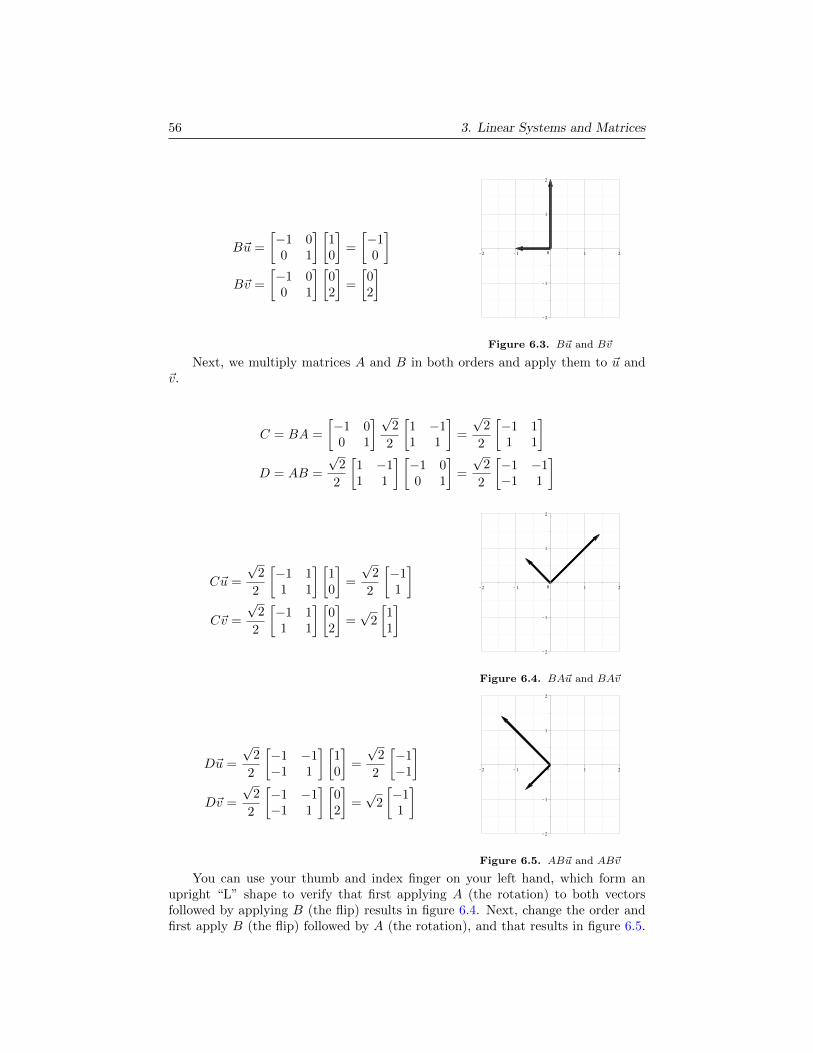
56 3. Linear Systems and Matrices
B~u =
[−1 00 1
] [10
]=
[−10
]B~v =
[−1 00 1
] [02
]=
[02
]
Figure 6.3. B~u and B~v
Next, we multiply matrices A and B in both orders and apply them to ~u and~v.
C = BA =
[−1 00 1
] √2
2
[1 −11 1
]=
√2
2
[−1 11 1
]D = AB =
√2
2
[1 −11 1
] [−1 00 1
]=
√2
2
[−1 −1−1 1
]
C~u =
√2
2
[−1 11 1
] [10
]=
√2
2
[−11
]C~v =
√2
2
[−1 11 1
] [02
]=√
2
[11
]
Figure 6.4. BA~u and BA~v
D~u =
√2
2
[−1 −1−1 1
] [10
]=
√2
2
[−1−1
]D~v =
√2
2
[−1 −1−1 1
] [02
]=√
2
[−11
]
Figure 6.5. AB~u and AB~v
You can use your thumb and index finger on your left hand, which form anupright “L” shape to verify that first applying A (the rotation) to both vectorsfollowed by applying B (the flip) results in figure 6.4. Next, change the order andfirst apply B (the flip) followed by A (the rotation), and that results in figure 6.5.
7. Inverses of Matrices 57
Recall that function application is read from left to right, so AB~u corresponds tofirst applyingB and then applyingA. Adding parentheses may help: AB~u = A(B~u)
4
7. Inverses of Matrices
Perhaps the most common problem in algebra is solving an equation. But you’veprobably never thought much about exactly what algebraic properties of arithmeticallow us to solve as simple an equation as 2x = 3. Undoubtedly, you can look at theequation and quickly arrive at an answer of x = 3/2, but what are the underlyingalgebraic principles which you are subconsciously employing to allow you to drawthat conclusion?
Suppose a, b are real numbers, can we always solve the equation:
ax = b
for any unknown x?
No, not always. For example if a = 0 and b 6= 0, then there is no solution. Thisis the only case that does not have a solution because 0 is the only real number thatdoes not have a multiplicative inverse. Assuming a 6= 0, you solve the equation inthe following manner:
ax = b
a−1(ax) = a−1b (existence of multiplicative inverses)
(a−1a)x = a−1b (associativity of multiplication)
1x = a−1b (multiplicative inverse property)
x = a−1b (multiplicative identity property)
Notice that we never needed to use the commutative property of multiplicationnor distributivity. Associativity, inverses, and identity form the core of any algebraicsystem.
Now we wish to solve matrix equations in a similar fashion, i.e. we wish tosolve matrix equations by multipying both sides of an equation by the inverse of amatrix, e.g.
A~x = ~b
A−1(A~x) = A−1~b
(A−1A)~x = A−1~b
I~x = A−1~b
~x = A−1~b
where A is a matrix and ~x and ~b are vectors. Since matrix multiplication isthe same as composition of maps (functions), this method of solution amounts to
finding the inverse of the map A and then applying it to the vector ~b.
However, not all matrices have an inverse.
58 3. Linear Systems and Matrices
7.1. Inverse of a General 2× 2 Matrix. In what follows, we will often need tocompute the inverse of 2×2 matrix. It will save time if we can generate a formula orsimple rule for determining when such a matrix is invertible and what the inverse is.To derive such a formula, we must compute the inverse of the matrix: A =
[a bc d
].
a b 1 0
c d 0 1
1aR1−→
1 ba
1a 0
c d 0 1
−→−cR1+R2
1 ba
1a 0
0 ad−bca − c
a 1
−→a
ad−bcR21 ba
1a 0
0 1 − cad−bc
aad−bc
− baR2+R1−→
1 0 dad−bc − b
ad−bc
0 1 − cad−bc
aad−bc
Thus the inverse of A is:
A−1 =1
ad− bc
[d −b−c a
]Clearly, we will not be able to invert A if ad − bc = 0, thus we have found thecondition for the genral 2×2 matrix which determines whether or not it is invertible.
8. Determinants
The determinant is a function which takes a square, n × n matrix and returns areal number. If we let Mn(R) denote the set of all n×n matrices with entries fromR, then the determinant function has the following signature:
det : Mn(R)→ R.We denote this function two ways, det(A) = |A|. The algorithm for computingthis function is defined recursively, similar to how the elimination algorithm wasdefined. Thus the first definition below, the definition for the minor of a matrixwill use the term determinant which is defined later. This is just the nature ofrecursive algorithms.
Definition 3.13. The ijth minor of a matrix A, denoted Mij , is the determinantof the matrix A with its ith row and jth column removed.
For example, if A is a 4× 4 matrix, then M23 is:
M23 =
∣∣∣∣∣∣∣∣a11 a12 a13 a14
a21 a22 a23 a24
a31 a32 a33 a34
a41 a42 a43 a44
∣∣∣∣∣∣∣∣ =
∣∣∣∣∣∣a11 a12 a14
a31 a32 a34
a41 a42 a44
∣∣∣∣∣∣Definition 3.14. The ijth cofactor of a matrix A, denoted Aij , is defined to be,
Aij = (−1)(i+j)Mij .
Notice that cofactors are defined in terms of minors. Next we define the deter-minant in terms of cofactors.
8. Determinants 59
Definition 3.15. The determinant function is defined recursively, so we need twocases, a base case and a recursive case.
• The determinant of a 1× 1 matrix or scalar is just the scalar.
• The determinant of a square, n× n matrix A, is
det(A) = a11A11 + a12A12 + · · ·+ a1nA1n.
Notice that a11, a12, . . . , a1n are just the elements in the first row of the matrixA. The A11, A12, . . . , A1n are cofactors of the matrix A. We call this a cofactorexpansion along the first row.
Let’s unwind the previous definitions to compute the determinant of the matrix,
A =
[a bc d
]det(A) = a11A11 + a12A12
= aA11 + bA12
= a(−1)(1+1)d+ b(−1)(1+2)c
= ad− bcNotice that this same quantity appeared when we found the inverse of A in theprevious section. This is no accident. The determinant is closely related to invert-ibility.
Example 3.16. Compute det(A), if A is the following matrix.
A =
1 0 30 −2 2−5 4 1
det(A) = a11A11 + a12A12 + a13A13
= a11(−1)1+1M11 + a12(−1)1+2M12 + a13(−1)1+3M13
= 1(−1)1+1
∣∣∣∣−2 24 1
∣∣∣∣+ 0(−1)1+2
∣∣∣∣ 0 2−5 1
∣∣∣∣+ 3(−1)1+3
∣∣∣∣ 0 −2−5 4
∣∣∣∣=
∣∣∣∣−2 24 1
∣∣∣∣+ 0 + 3
∣∣∣∣ 0 −2−5 4
∣∣∣∣Using the definition for the determinant of a 2 × 2 matrix found in the previoussection we get:
= −10 + 0 + 3(−10)
= −40
4
The recursive nature of the determinant makes it difficult to compute the deter-minants of large matrices even with computers. However, there are several key factsabout the determinant which make computations easier. Most computer systems
60 3. Linear Systems and Matrices
use the following theorem to make computing of determinants for large matricesfeasible.
Theorem 3.17 (Elementary Row Operations and the Determinant). Recall thereare three elementary row operations. They each affect the computation of |A| dif-ferently.
(1) Suppose B is obtained by swapping two rows of the matrix A, then
|B| = − |A| .(2) Suppose B is obtained by multiplying a row of matrix A by a nonzero constant
k, then|B| = k |A| .
(3) Suppose B is obtained by adding a multiple of one row to another row in matrixA, then
|B| = |A| .
Theorem 3.18 (Determinants of Matrix Products). If A and B are n×n matrices,then
|AB| = |A| |B|
Definition 3.19. The transpose of a matrix is obtained by changing its rows intocolumns, or vice versa, and keeping their order intact. The transpose of a matrixA is denoted AT .
Example 3.20. 2 1 00 0 72 −1 35 1 −2
T
=
2 0 2 51 0 −1 10 7 3 −2
4
Theorem 3.21 (Transpose Facts). The following properties of transposes are oftenuseful.
(1) (AT )T = A.
(2) (A+B)T = AT +BT
(3) (cA)T = c(AT )
(4) (AB)T = BTAT
Theorem 3.22 (Determinants of Transposed Matrices). If A is a square matrix,then det(AT ) = det(A).
8.1. Geometric Interpretation of Determinants.

Chapter 4
Vector Spaces
1. Basics
Definition 4.1. A vector is an ordered list of real numbers. Vectors will bedenoted by a lower case letter with an arrow over it, e.g. ~v = (
√2,−3, 0).
Definition 4.2 (n-space). Rn = (a1, a2, . . . , an) | ai ∈ R for i = 1 . . . n, whichin words reads: Rn (pronounced “r”, “n”) is the set of all vectors with n realcomponents.
Example 4.3. A vector in R2 is a pair of real numbers. For example (3, 2) is avector. We can interpret this pair in two ways:
(1) a point in the xy–plane, or
(2) an arrow whose tail is at the origin and whose tip is at (3, 2).
A vector in R3 is a triple of real numbers, and can be interpreted as a point(x, y, z) in space, or as an arrow whose tail is at (0, 0, 0) and whose tip is at (x, y, z)
4
We sometimes call a vector with n components an n–tuple. The “tuple” partof n–tuple comes from quadruple, quintuple, sextuple, septuple, etc..
In this chapter we will mostly use the arrow interpretation of vectors, i.e. thenotion of directional displacement. Since the arrow really only represents displace-ment, it doesn’t matter where we put the tail of the arrow. In fact you can translate(or move) a vector in R2 all around the plane and it remains the same vector, aslong as you don’t rotate it or scale it. Similarly for a vector with three componentsor any number of components for that matter. Thus the defining characteristic ofa vector is its direction and magnitude (or length).
Definition 4.4. The magnitude of a vector is the distance from the origin to thepoint in Rn the vector represents. Magnitude is denoted by |~v| and is computed
61
62 4. Vector Spaces
via the following generalization of the Pythagorean theorem:
|~v| =√v2
1 + v22 + · · ·+ v2
n =
(n∑i=1
v2i
) 12
Example 4.5. Given the vector ~v = (3,−2, 4) ∈ R3,
|~v| =√
32 + (−2)2 + 42 =√
29
4
Definition 4.6 (vector addition). Two vectors are added component–wise, mean-ing that given two vectors say, ~u = (u1, u2, . . . , un) and ~v = (v1, v2, . . . , vn), then
~u+ ~v = (u1 + v1, u2 + v2, . . . , un + vn).
Notice that this way of defining addition of vectors only makes sense if bothvectors have the same number of components.
Definition 4.7 (scalar multiplication). A vector can be scaled by any realnumber, meaning that if a ∈ R and ~u = (u1, u2, . . . , un), then
a~u = (au1, au2, . . . , aun).
Scaling literally corresponds to stretching or contracting the magnitude of thevector. Scaling by a negative number is scaling and reflecting. If the vector is apair, then the reflection corresponds to a reflection about the line y = −x whichwhen written in general form is x + y = 0. A reflection in 3–space corresponds toa reflection about the plane x+ y + z = 0, and so on and so forth.
Definition 4.8. A vector space is a nonempty set, V , of vectors, along with theoperations of vector addition, and scalar multiplication which satisfies the followingrequirements for all ~u,~v, ~w ∈ V , and for all scalars a, b ∈ R.
(1) ~u+ ~v = ~v + ~u (commutativity)
(2) (~u+ ~v) + ~w = ~u+ (~v + ~w) (additive associativity)
(3) ~v +~0 = ~v (additive identity)
(4) ~v +−~v = ~0 (additive inverses)
(5) a(~u+ ~v) = a~u+ a~v (distributivity over vector addition)
(6) (a+ b)~u = a~u+ b~u (distributivity over scalar addition)
(7) (ab)~u = a(b~u) (multiplicative associativity)
(8) 1~u = ~u (multiplicative identity)

1. Basics 63
Remark 4.9. Notice that the definition for a vector space does not require a wayof multiplying two vectors to yield another vector. If you studied multi–variablecalculus then you may be familiar with the cross product, which is a form of vectormultiplication, but the definition of a vector space does not mention the crossproduct. However, being able to scale vectors by real numbers is a vital piece ofthe vector space definition.
A vector space is probably your first introduction to a mathematical definitioninvolving a “set with structure”. The structure here is provided by the operationsof vector addition and scalar mulitplication, as well as the eight requirements thatthey must satisfy. We will see at the end of this chapter that a vector space isn’tdefined by the objects in the set as much as by the rigid relationships between theseobjects that the eight requirements enforce.
In short, a vector space is a nonempty set that is closed under vector additionand scalar multiplication. Here, “closed” means that if you take any two vectors inthe vector space and add them, then their sum will also be a vector in the vectorspace. Likewise if you scale any vector in the vector space, then the scaled versionwill also be an element of the vector space.
Definition 4.10. A linear combination of vectors is a scaled sum of vectors.For example, a linear combination of the vectors ~v1, ~v2, . . . , ~vn could be written:c1~v1 + c2~v2 + · · ·+ cn~vn, where c1, c2, . . . , cn are real numbers (scalars).
The concept defined above, of generating a new vector from other vectors is afoundational concept in the study of Linear Algebra. It will occur throughout therest of this book.
Given this definition, one can think of a vector space as a nonempty set ofvectors that is closed under linear combinations. Which is to say that any linearcombination of vectors from a vector space will again be an element of the vectorspace. You may be wondering why we make the requirement that a vector spacemust be a nonempty set. This is because every vector space must contain the zerovector, ~0. Since vector spaces are closed under scalar multiplication, any nonemptyvector space will necessarily contain the zero vector. This is because you can alwaystake any vector and scale it by the scalar, 0, to get the vector, ~0. As we developthe theory, you will see that it makes more sense for the set ~0 to be the smallestpossible vector space rather than the empty set . This is the reason for requiringvector spaces to be nonempty.
Linear combinations are important because they give us a new geometric per-spective on the calculations we did in the previous chapter.
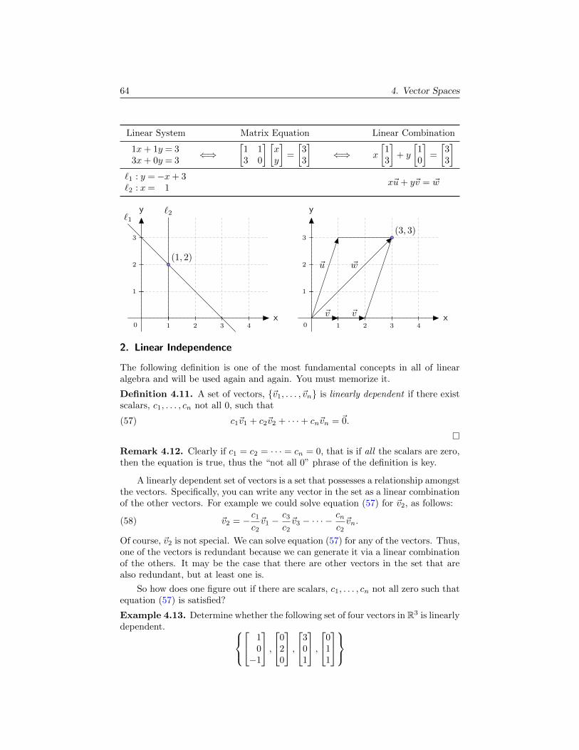
64 4. Vector Spaces
Linear System Matrix Equation Linear Combination
1x+ 1y = 33x+ 0y = 3
⇐⇒[1 13 0
] [xy
]=
[33
]⇐⇒ x
[13
]+ y
[10
]=
[33
]`1 : y =−x+ 3`2 : x= 1
x~u+ y~v = ~w
1 2 3 4x
1
2
3
y
0
`1`2
(1, 2)
1 2 3 4x
1
2
3
y
0
(3, 3)
~u
~v ~v
~w
2. Linear Independence
The following definition is one of the most fundamental concepts in all of linearalgebra and will be used again and again. You must memorize it.
Definition 4.11. A set of vectors, ~v1, . . . , ~vn is linearly dependent if there existscalars, c1, . . . , cn not all 0, such that
(57) c1~v1 + c2~v2 + · · ·+ cn~vn = ~0.
Remark 4.12. Clearly if c1 = c2 = · · · = cn = 0, that is if all the scalars are zero,then the equation is true, thus the “not all 0” phrase of the definition is key.
A linearly dependent set of vectors is a set that possesses a relationship amongstthe vectors. Specifically, you can write any vector in the set as a linear combinationof the other vectors. For example we could solve equation (57) for ~v2, as follows:
(58) ~v2 = −c1c2~v1 −
c3c2~v3 − · · · −
cnc2~vn.
Of course, ~v2 is not special. We can solve equation (57) for any of the vectors. Thus,one of the vectors is redundant because we can generate it via a linear combinationof the others. It may be the case that there are other vectors in the set that arealso redundant, but at least one is.
So how does one figure out if there are scalars, c1, . . . , cn not all zero such thatequation (57) is satisfied?
Example 4.13. Determine whether the following set of four vectors in R3 is linearlydependent.
10−1
,0
20
,3
01
,0
11
4. Affine Spaces 65
We must figure out if there exist scalars c1, c2, c3, c4 not all zero such that
(59) c1
10−1
+ c2
020
+ c3
301
+ c4
011
=
000
.Let’s rewrite the last equation by absorbing the scalars into the vectors and sum-ming them: 1 · c1 + 0 · c2 + 3 · c3 + 0 · c4
0 · c1 + 2 · c2 + 0 · c3 + 1 · c4−1 · c1 + 0 · c2 + 1 · c3 + 1 · c4
=
000
.The last equation corresponds to a linear system of three equations in four unknownsc1, . . . , c4! 1c1 + 0c2 + 3c3 + 0c4 = 0
0c1 + 2c2 + 0c3 + 1c4 = 0−1c1 + 0c2 + 1c3 + 1c4 = 0
And this system of equations can be written as a coefficient matrix times a columnvector of the unknowns:
(60)
1 0 3 00 2 0 1−1 0 1 1
c1c2c3c4
=
000
.Equations (59) and (60) are two different ways of writing the exact same thing!
In other words, multiplying a matrix by a column vector is equivalent to makinga linear combination of the columns of the matrix. The columns of the matrix inequation (60) are exactly the vectors of equation (59).
We can write this as an augmented matrix and perform elemetary row oper-ations to determine the solution set if any. However, since it is a homogeneoussystem, no matter what elementary row ops we apply, the rightmost column willalways remain as all zeros, thus there is no point in writing it. Instead we onlyneed to perform row ops on the coefficient matrix.
4
3. Vector Subspaces
4. Affine Spaces
There is an interesting connection between solutions to homogeneous and nonho-mogeneous linear systems.
Lemma 4.14. If ~u and ~v are both solutions to the nonhomogeneous equation,
(61) A~x = ~b,
then their difference ~y = ~u− ~v is a solution to the associated homogeneous system:
(62) A~x = ~0,

66 4. Vector Spaces
Proof. This is a simple consequence of the fact that matrix multiplication dis-tributes over vector addition.
A~y = A(~u− ~v)
= A~u−A~v
= ~b−~b
= ~0
This idea of the lemma is illustrated in figure 4.1 for the system:
(63)
[1 20 0
] [xy
]=
[120
],
which has the following associated homogeneous system:
(64)
[1 20 0
] [xy
]=
[00
].
−4 −2 2 4 6 8 10 12
x
−2
2
4
6
y
0
x+ 2y = 12
x+ 2y = 0
(4, 4)
~u (8, 2)
~v
(4,−2)
~v − ~u
(−4, 2)
~u− ~v
Figure 4.1. Affine solution space for equation 63 and vector subspace of
solutions to equation 64.
5. Bases and Dimension
We know that a vector space is simply a nonempty set of vectors that is closed undertaking linear combinations, a natural question to ask is, “Is there some subset ofvectors which allow us to generate (via linear combinations) every vector in thevector space?”. Since a set is always considered a subset of itself, the answer tothis question is clearly yes, because the vector space itself can generate any vectorin the vector space. But can we find a proper subset, or perhaps even a finite

6. Abstract Vector Spaces 67
subset from which we can generate all vectors in the vector space by taking linearcombinations?
The answer to this question is yes, in fact such a set exists for every vectorspace, although it might not always be finite.
6. Abstract Vector Spaces
When we first defined a vector, we defined it to be an ordered list of real numbers,and we noted that the definining characteristic was that a vector had a directionand a magnitude. We then proceeded to define a vector space as a set of objectsthat obeyed eight rules. These eight rules revolved around addition or summingand multiplication or scaling. Finally, we observed that all but one of these eightrules could be summed up by saying that a vector space is a nonempty set of vectorsthat is closed under linear combinations (scaled sums). Where “closed” meant thatif ~u,~v ∈ V , then ~u + ~v ∈ V and if c ∈ R, then c~v ∈ V . The one vector spacerequirement that this “definition” does not satisfy is the very first requirement thataddition must be commutative, i.e. ~u + ~v = ~v + ~u for all ~u,~v ∈ V . It turns outthat vector spaces are ubiquitous in mathematics. This section will give severalexamples.
Example 4.15 (Matrices as a Vector Space). Consider the set of m× n matriceswith real entries which we will denote, Mmn(R). This set is a vector space. To seewhy let A,B be elements of Mmn(R), and let c be any real number then
(1) Mmn(R) is not empty, specifically it contains an m × n matrix made of allzeros which serves as our zero vector.
(2) This set is closed under addition, A+B ∈Mmn(R).
(3) This set is closed under scalar multiplication, cA ∈Mmn(R).
(4) Matrix addition is commutative, A+B = B +A for all matrices in Mmn(R).
More concretely, consider M22(R), the set of 2×2 matrices with real entries. Whatsubset of M22(R), is a basis for this vector space? Well, whatever it is it must allowus to write any matrix as a linear combination of its elements. The simplest choiceis called the standard basis, and in this case the simplest choice is the set:
B =
[1 00 0
],
[0 10 0
],
[0 01 0
],
[0 00 1
]This allow us to write for example,[
a bc d
]= a
[1 00 0
]+ b
[0 10 0
]+ c
[0 01 0
]+ d
[0 00 1
]Is B really a basis? Clearly it spans the vector space M22(R), but is there perhaps asmaller set which still spans M22(R)? Also, how do we know that the four matricesin B are linearly independent? 4
Example 4.16 (Solution Space of Homogeneous, Linear Differential Equations).Consider the differential equation
(65) y′′ + y = 0.

68 4. Vector Spaces
You can check that both
y1 = cosx, and
y2 = sinx
are solutions. But also, any linear combination of these two solutions is again asolution. To see this let y = ay1 + by2 where a and b are scalars, then:
y = a cosx+ b sinx
y′ = −a sinx+ b cosx
y′′ = −a cosx− b sinx
So y′′ + y = (−a cosx − b sinx) + (a cosx + b sinx) = 0, and thus we see that theset of solutions is nonempty and closed under linear combinations and therefore avector space. 4
Notice that if equation (65) were not homogeneous, that is if the right handside of the equation were not zero, then the set of solutions would not form a vectorspace.
Example 4.17 (Solution Space of Nonhomogeneous, Linear Differential Equa-tions). Consider the differential equation
(66) y′′ + y = ex.
You can check that both
y1 = cosx+1
2ex, and
y2 = sinx+1
2ex
are solutions. However, linear combinations of these two solutions are not solutions.To see this let y = ay1 + by2 where a and b are scalars, then:
y = a
(cosx+
1
2ex)
+ b
(sinx+
1
2ex)
y′ = a
(− sinx+
1
2ex)
+ b
(cosx+
1
2ex)
y′′ = a
(− cosx+
1
2ex)
+ b
(− sinx+
1
2ex)
y′′ + y = a1
2ex + b
1
2ex + a
1
2ex + b
1
2ex
= (a+ b)ex
Thus y1 and y2 will only be solutions when a+ b = 1. 4

Chapter 5
Higher Order LinearDifferential Equations
1. Homogeneous Differential Equations
Similar to how homogeneous systems of linear equations played an important rolein developing the theory of vector spaces, a similar class of differential equationswill be instrumental in understanding the theory behind solving higher order lineardifferential equations.
Recall definition 1.25, which states that a differential equation is defined to belinear if it can be written in the form:
(22) an(x)y(n) + an−1(x)y(n−1) + · · ·+ a1(x)y′ + a0(x)y = f(x).
Definition 5.1. A linear differential equation is called homogeneous if f(x) = 0.That is if it can be written in the form:
(67) an(x)y(n) + an−1(x)y(n−1) + · · ·+ a1(x)y′ + a0(x)y = 0.
where the right hand side of the equation is exactly zero.
Similar to how the solution space of a homogeneous system of linear equationsformed a vector subspace of Rn, the solutions of linear, homogeneous differentialequations form a vector subspace of F the vector space of functions of a real variable.
Theorem 5.2. The set of solutions to a linear homogeneous differential equation(equation 67) form a vector subspace of F , the set of all functions of a real variable.
Proof. For sake of simplicity, we will only prove this for a general second order,homogeneous differential equation such as:
(68) a2(x)y′′ + a1(x)y′ + a0(x)y = 0.
The necessary modifications for a general nth order equation are left as an exercise.
69

70 5. Higher Order Linear Differential Equations
Let V be the set of all solutions to equation 68. We must show three things:1) V is nonempty, 2) V is closed under vector addition, 3) V is closed under scalarmultiplication.
(1) Clearly the function y(x) ≡ 0 is a solution to equation 68, thus V is nonempty.
(2) Let y1, y2 ∈ V and let y = y1 + y2. If we plug this into equation 68 we get:
a2(x)y′′ + a1(x)y′ + a0(x)y
= a2(x)(y1 + y2)′′ + a1(x)(y1 + y2)′ + a0(x)(y1 + y2)
= a2(x)(y′′1 + y′′2 ) + a1(x)(y′1 + y′2) + a0(x)(y1 + y2)
= [a2(x)y′′1 + a1(x)y′1 + a0(x)y1] + [a2(x)y′′2 + a1(x)y′2 + a0(x)y2]
= 0
(3) Let y1 ∈ V, α ∈ R and let y = αy1. If we plug y into equation 68 we get:
a2(x)(αy1)′′ + a1(x)(αy1)′ + a0(x)(αy1)
= αa2(x)y′′1 + αa1(x)y′1 + αa0(x)y1
= α[a2(x)y′′1 + a1(x)y′1 + a0(x)y1]
= 0
Now that we know that the set of solutions of a linear, homogeneous equationform a vector space, the next obvious thing to do is figure out a way to generate abasis for the solution space. Then we will be able to write the general solution asa linear combination of the basis functions. For example, suppose a basis containsthree functions y1(x), y2(x) and y3(x), then a general solution would have the form:
c1y1(x) + c2y2(x) + c3y3(x).
At this point we don’t even know how to determine the dimension of a basis forthe solution space let alone actual basis functions. Thus, it makes sense to imposesome simplifying assumptions. Instead of considering general nth order, linear,homogeneous equations like equation 67, let’s only consider second order equations.In fact, it will be advantageous to be even more restrictive, let’s only considerequations with constant coefficients. Thus let’s consider DEs of the form:
(69) y′′ + ay′ + by = 0,
where a and b are elements of R, the set of real numbers.
2. Linear Equations with Constant Coefficients
2.1. Linear Operators. If we let D = ddx , and let D2 = d2
dx2 , then we can writeequation 69 like so,
(70) D2y + aDy + by = 0.
Each term on the left now involves y, instead of different derivatives of y. Thisallows us to rewrite the equation as:
(71) (D2 + aD + b)y = 0.
2. Linear Equations with Constant Coefficients 71
Equation 71 deserves some explanation. It is analogous to the matrix equation:
(A2 + aA+ b)~v = A2~v + aA~v + b~v = ~0,
where we have replaced differention, (D) with a square matrix A and the functiony is replaced with the vector, ~v. The expression (D2 + aD + b) is a function withdomain F and codomain (range) also F . In other words it is a function on functions.You should already be familiar with the notion of the derivative as a function onfunctions. The only thing new we have introduced is combining multiple derivativesalong with scalars into a single function. Also, we are using multiplicative notationto denote function application. That is, we will usually forgo the parentheses in(D2 + aD + b)(y) in favor of (D2 + aD + b)y. Thus we can rewrite a second order,linear, homogeneous DE with constant coefficients in two equivalent ways:
y′′ + ay′ + by = 0 ⇐⇒ (D2 + aD + b)y = 0.
Finally, if we let
(72) L = D2 + aD + b,
then we can write equation 69 very compactly:
Ly = 0.
Solving this DE amounts to figuring out the set of functions which get mapped tothe zero function, by the linear operator L = D2 + aD + b.
Definition 5.3. A linear operator is a function often denoted L with signature:
L : F → F
that is, it is a function which maps functions to other functions such that
L(c1y1 + c2y2) = c1Ly1 + c2Ly2,
where c1, c2 are scalars and y1, y2 are functions.
Remark 5.4. The linear operator notation: (D2 +aD+ b) is simply shorthand fora function on functions. In other words it is a name for a function similar to how wemight associate the symbol f with the expression x2 + 1 by writing f(x) = x2 + 1.The difference is that the name also serves as the function definition.
Remark 5.5. The linear operator notation: (D2 + aD + b) does not representan expression that can be evaluated. Recall that this is analogous to the matrixequation A2 + aA + b, but although the sum A2 + aA is defined for square n × nmatrices the second sum, aA + b is not even defined. For example, it makes nosense to add a 2 × 2 matrix to a scalar. Similarly it makes no sense to add thederivative operator to a scalar. However it does make sense to add the derivativeof a function to a scalar multiple of a function.
Of course, this notation works for first order and higher order differential equa-tions as well. For example,
y′ − 3y = 0 ⇐⇒ (D − 3)y = 0,
y(4) + 6y′′ + 12y = 0 ⇐⇒ (D4 + 6D2 + 12)y = 0.
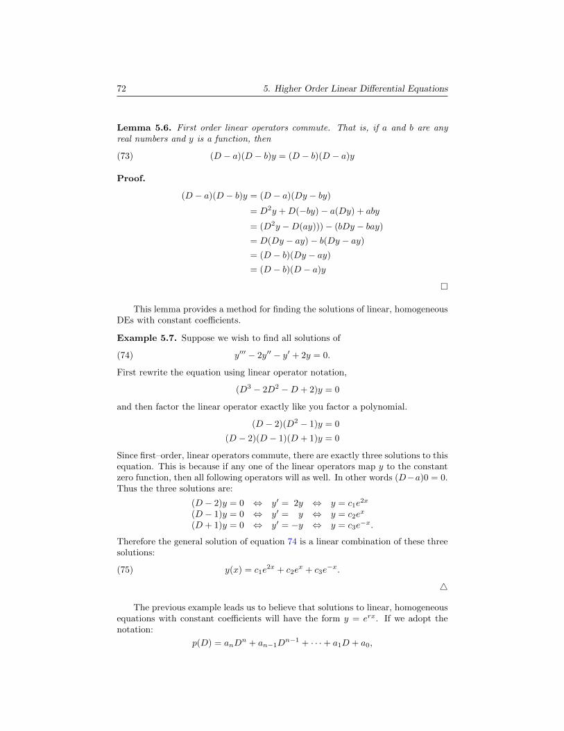
72 5. Higher Order Linear Differential Equations
Lemma 5.6. First order linear operators commute. That is, if a and b are anyreal numbers and y is a function, then
(73) (D − a)(D − b)y = (D − b)(D − a)y
Proof.
(D − a)(D − b)y = (D − a)(Dy − by)
= D2y +D(−by)− a(Dy) + aby
= (D2y −D(ay)))− (bDy − bay)
= D(Dy − ay)− b(Dy − ay)
= (D − b)(Dy − ay)
= (D − b)(D − a)y
This lemma provides a method for finding the solutions of linear, homogeneousDEs with constant coefficients.
Example 5.7. Suppose we wish to find all solutions of
(74) y′′′ − 2y′′ − y′ + 2y = 0.
First rewrite the equation using linear operator notation,
(D3 − 2D2 −D + 2)y = 0
and then factor the linear operator exactly like you factor a polynomial.
(D − 2)(D2 − 1)y = 0
(D − 2)(D − 1)(D + 1)y = 0
Since first–order, linear operators commute, there are exactly three solutions to thisequation. This is because if any one of the linear operators map y to the constantzero function, then all following operators will as well. In other words (D−a)0 = 0.Thus the three solutions are:
(D − 2)y = 0 ⇔ y′ = 2y ⇔ y = c1e2x
(D − 1)y = 0 ⇔ y′ = y ⇔ y = c2ex
(D + 1)y = 0 ⇔ y′ = −y ⇔ y = c3e−x.
Therefore the general solution of equation 74 is a linear combination of these threesolutions:
(75) y(x) = c1e2x + c2e
x + c3e−x.
4
The previous example leads us to believe that solutions to linear, homogeneousequations with constant coefficients will have the form y = erx. If we adopt thenotation:
p(D) = anDn + an−1D
n−1 + · · ·+ a1D + a0,

2. Linear Equations with Constant Coefficients 73
then we see that we can write a homogeneous linear equation as p(D)y = 0. In par-ticular, we can write second order, homogeneous, linear equations in the followingway
a2y′′ + a1y
′ + a0y = 0
(a2D2 + a1D + a0)y = 0
p(D)y = 0
This means that we can interpret p(D) as a linear operator.
2.2. Repeated Roots. What if our linear operator has a repeated factor? Forexample (D − r)(D − r)y = 0, does this mean that the differential equation
(76) (D − r)2y = 0 ⇐⇒ y′′ − 2ry′ + r2y = 0
only has solution y1 = erx? This is equivalent to saying that the solution space isone dimensional. But could the solution space still be two dimensional? Let’s guessthat there is another solution y2 of the form
y2 = u(x)y1,
where u(x) is some undetermined function, but with the restriction u(x) 6≡ c. Wemust not allow u(x) to be a constant function, otherwise y1 and y2 will be linearlydependent and will not form a basis for the solution space.
(D − r)2y2 = (D − r)2u(x)y1
= (D − r)2u(x)erx
= (D − r)[(D − r)u(x)erx]
= (D − r)[Du(x)erx − ru(x)erx]
= (D − r)[u′(x)erx + ru(x)erx − ru(x)erx]
= (D − r)[u′(x)erx]
= D[u′(x)erx]− ru′(x)erx
= u′′(x)erx + ru′(x)erx − ru′(x)erx
= u′′(x)erx
= [D2u(x)]erx = 0.
It follows that if y2 = u(x)y1(x) is to be a solution of equation 76, then:
D2u(x) = 0.
In other words u(x) must satisfy u′′(x) = 0. We already know that degree onepolynomials satisfy this constraint. Thus u(x) can be any linear polynomial, forexample:
u(x) = a0 + a1x.
Hence y2(x) = (a0 +a1x)erx and thus our general solution to equation 76 is a linearcombination of the two solutions y1 and y2:

74 5. Higher Order Linear Differential Equations
y = c1y1 + c2y2
= c1erx + c2(a0 + a1x)erx
= c1erx + c2 · a0e
rx + c2 · a1xerx
= (c1 + c2 · a0)erx + (c2 · a1)xerx
= (c∗1 + c∗2x)erx
Notice that the general solution is equivalent to y2 alone. Since y2 necessarily hastwo unknowns in it (a0 and a1 from the linear polynomial), this is reasonable. Hencethe general solution to a second order, linear equation with the single repeated rootr in its characteristic equation is given by:
y = (c1 + c2x)erx.
The steps above can be extended to the situation where a linear operator con-sists of a product of k equal first order linear operators.
Lemma 5.8. If the characteristic equation of a linear, homogeneous differentialequation with constant coefficients has a repeated root of multiplicity k, for example
(77) (D − r1)(D − r2) · · · (D − rn)(D − r)ky = 0,
then the part of the general solution corresponding to the root r has the form
(78) (c1 + c2x+ c3x2 + · · ·+ ckx
k−1)erx.
2.3. Complex Conjugate Roots.
3. Mechanical Vibrations
A good physical example of a second order, linear differential equation with constantcoefficients is provided by a mass, spring and dashpot setup as depicted below. Adashpot is simply a piston like device which provides resistance proportional to therate at which it is compressed or pulled. It is like the shock absorbers found incars. In this setup there are three separate forces acting on the mass.
mk c
Figure 3.1. Mass, spring, dashpot mechanical system
(1) Spring: Fs = −kx(2) Dashpot: Fd = −cx′
(3) Driving Force: F (t)
The spring provides a restorative force meaning that its force is proportional tobut in the opposite direction of the displacement of the mass. Similarly, the forcedue to the dashpot is proportional to the velocity of the mass, but in the oppositedirection. Finally, the driving force could correspond to any function we are capable
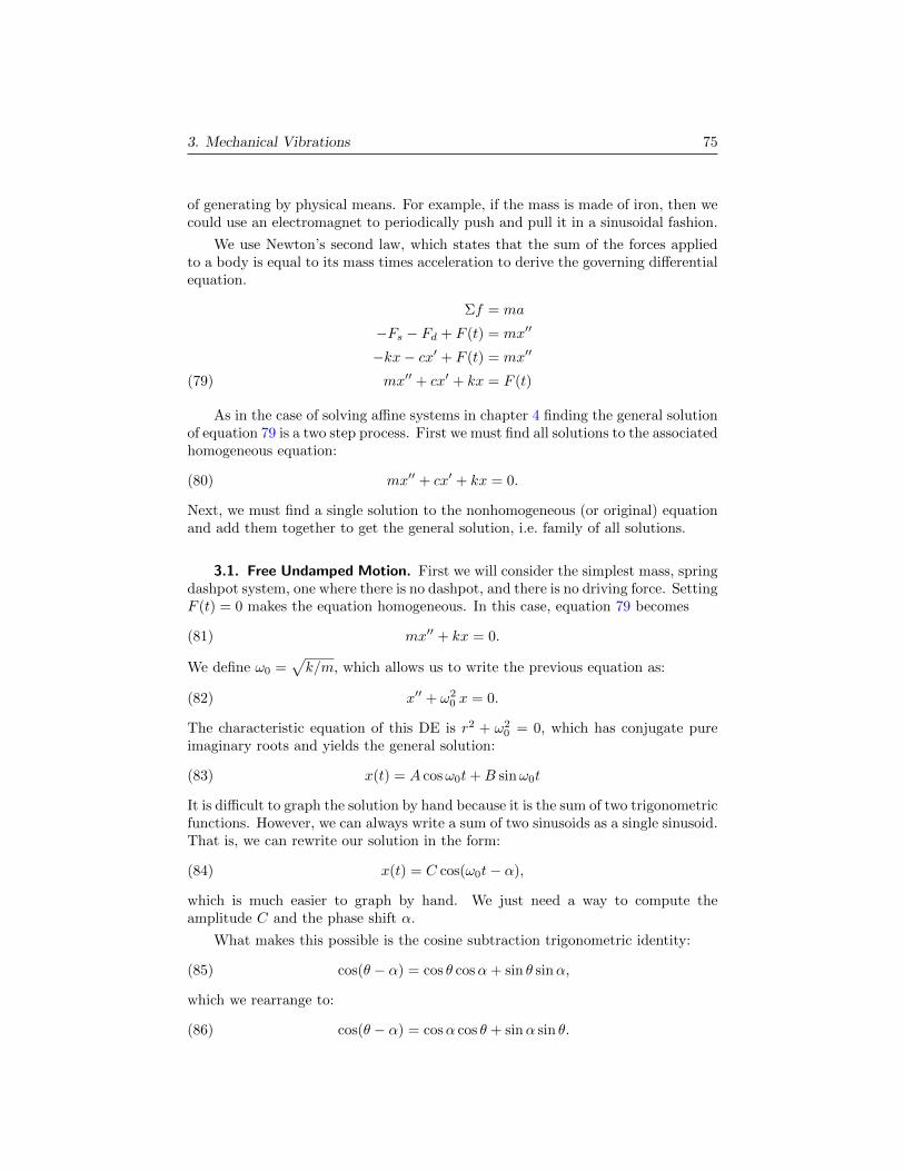
3. Mechanical Vibrations 75
of generating by physical means. For example, if the mass is made of iron, then wecould use an electromagnet to periodically push and pull it in a sinusoidal fashion.
We use Newton’s second law, which states that the sum of the forces appliedto a body is equal to its mass times acceleration to derive the governing differentialequation.
Σf = ma
−Fs − Fd + F (t) = mx′′
−kx− cx′ + F (t) = mx′′
mx′′ + cx′ + kx = F (t)(79)
As in the case of solving affine systems in chapter 4 finding the general solutionof equation 79 is a two step process. First we must find all solutions to the associatedhomogeneous equation:
(80) mx′′ + cx′ + kx = 0.
Next, we must find a single solution to the nonhomogeneous (or original) equationand add them together to get the general solution, i.e. family of all solutions.
3.1. Free Undamped Motion. First we will consider the simplest mass, springdashpot system, one where there is no dashpot, and there is no driving force. SettingF (t) = 0 makes the equation homogeneous. In this case, equation 79 becomes
(81) mx′′ + kx = 0.
We define ω0 =√k/m, which allows us to write the previous equation as:
(82) x′′ + ω20 x = 0.
The characteristic equation of this DE is r2 + ω20 = 0, which has conjugate pure
imaginary roots and yields the general solution:
(83) x(t) = A cosω0t+B sinω0t
It is difficult to graph the solution by hand because it is the sum of two trigonometricfunctions. However, we can always write a sum of two sinusoids as a single sinusoid.That is, we can rewrite our solution in the form:
(84) x(t) = C cos(ω0t− α),
which is much easier to graph by hand. We just need a way to compute theamplitude C and the phase shift α.
What makes this possible is the cosine subtraction trigonometric identity:
(85) cos(θ − α) = cos θ cosα+ sin θ sinα,
which we rearrange to:
(86) cos(θ − α) = cosα cos θ + sinα sin θ.
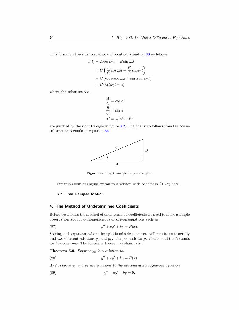
76 5. Higher Order Linear Differential Equations
This formula allows us to rewrite our solution, equation 83 as follows:
x(t) = A cosω0t+B sinω0t
= C
(A
Ccosω0t+
B
Csinω0t
)= C (cosα cosω0t+ sinα sinω0t)
= C cos(ω0t− α)
where the substitutions,
A
C= cosα
B
C= sinα
C =√A2 +B2
are justified by the right triangle in figure 3.2. The final step follows from the cosinesubtraction formula in equation 86.
A
BC
α
Figure 3.2. Right triangle for phase angle α
Put info about changing arctan to a version with codomain (0, 2π) here.
3.2. Free Damped Motion.
4. The Method of Undetermined Coefficients
Before we explain the method of undetermined coefficients we need to make a simpleobservation about nonhomogeneous or driven equations such as
(87) y′′ + ay′ + by = F (x).
Solving such equations where the right hand side is nonzero will require us to actullyfind two different solutions yp and yh. The p stands for particular and the h standsfor homogeneous. The following theorem explains why.
Theorem 5.9. Suppose yp is a solution to:
(88) y′′ + ay′ + by = F (x).
And suppose y1 and y2 are solutions to the associated homogeneous equation:
(89) y′′ + ay′ + by = 0.
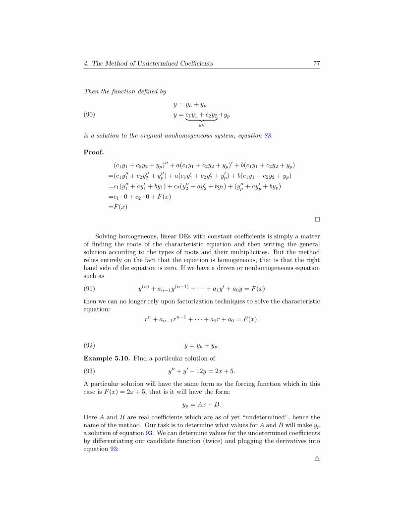
4. The Method of Undetermined Coefficients 77
Then the function defined by
y = yh + yp
y = c1y1 + c2y2︸ ︷︷ ︸yh
+yp(90)
is a solution to the original nonhomogeneous system, equation 88.
Proof.
(c1y1 + c2y2 + yp)′′ + a(c1y1 + c2y2 + yp)
′ + b(c1y1 + c2y2 + yp)
=(c1y′′1 + c2y
′′2 + y′′p ) + a(c1y
′1 + c2y
′2 + y′p) + b(c1y1 + c2y2 + yp)
=c1(y′′1 + ay′1 + by1) + c2(y′′2 + ay′2 + by2) + (y′′p + ay′p + byp)
=c1 · 0 + c2 · 0 + F (x)
=F (x)
Solving homogeneous, linear DEs with constant coefficients is simply a matterof finding the roots of the characteristic equation and then writing the generalsolution according to the types of roots and their multiplicities. But the methodrelies entirely on the fact that the equation is homogeneous, that is that the righthand side of the equation is zero. If we have a driven or nonhomogeneous equationsuch as
(91) y(n) + an−1y(n−1) + · · ·+ a1y
′ + a0y = F (x)
then we can no longer rely upon factorization techniques to solve the characteristicequation:
rn + an−1rn−1 + · · ·+ a1r + a0 = F (x).
(92) y = yh + yp.
Example 5.10. Find a particular solution of
(93) y′′ + y′ − 12y = 2x+ 5.
A particular solution will have the same form as the forcing function which in thiscase is F (x) = 2x+ 5, that is it will have the form:
yp = Ax+B.
Here A and B are real coefficients which are as of yet “undetermined”, hence thename of the method. Our task is to determine what values for A and B will make ypa solution of equation 93. We can determine values for the undetermined coefficientsby differentiating our candidate function (twice) and plugging the derivatives intoequation 93:
4

78 5. Higher Order Linear Differential Equations
5. The Method of Variation of Parameters
The method of undetermined coefficients examined in the previous section reliedupon the fact that the forcing function f(x) on the right hand side of the differentialequation had a finite number of linearly independent derivatives. What if this isn’tthe case? For example consider the equation
(94) y′′ + P (x)y′ +Q(x)y = tanx.
The derivatives of tanx are as follows:
sec2 x, 2 sec2 x tanx, 4 sec2 x tan2 x+ 2 sec4 x, . . .
These functions are all linearly independent. In fact, tanx has an infinite numberof linearly independent derivatives. Thus, clearly, the method of undeterminedcoefficients won’t work as a solution method for equation 94.
The method of variation of parameters can handle this situation. It is a moregeneral solution method, so in principle it can be used to solve any linear, non–homogeneous differential equation, but the method does force us to compute indef-inite integrals, so it does not always yield closed form solutions. However, it willallow us to solve linear equations with non–constant coefficients such as:
(95) y(n) + pn−1(x)y(n−1 + · · ·+ p2(x)y′′ + p1(x)y′ + p0(x)y = f(x)
Recall that the general solution to equation 95 will have the form
y = yh + yp
where yh is a solution to the associated homogeneous equation and is obtained viamethods explained previously if the coefficients are all constant. If they are notall constants, then your only recourse at this point will be trial and error. Thismethod assumes we already have a set of n linearly independent solutions to theassociated homogeneous equation. The method of variation of parameters is onlya method for finding a particular solution, yp.
For sake of simplicity, we first derive the formula for a general second orderlinear equation, such as:
(96) y′′ + P (x)y′ +Q(x)y = f(x).
We begin by assuming, or guessing that a particular solution might have the form
(97) yp = u1(x)y1 + u2(x)y2,
where u1, u2 are unknown functions, and y1 and y2 are known, linearly independentsolutions to the homogeneous equation associated with equation 96.
Our goal is to determine u1 and u2. Since we have two unknown functions,we will need two equations which these functions must satisfy. One equation isobvious, our guess for yp must satisfy equation 96, but there is no other obviousequation. However, when we plug our guess for yp into equation 96, then we willfind another equation which will greatly simplify the calculations.

5. The Method of Variation of Parameters 79
Before we can plug our guess for yp into equation 96 we need to compute twoderivatives of yp:
y′p = u′1y1 + u1y′1 + u′2y2 + u2y
′2
y′p = (u1y′1 + u2y
′2) + (u′1y1 + u′2y2).
Since we have the freedom to impose one more equation’s worth of restrictions onu1 and u2, it makes sense to impose the following condition:
(*) u′1y1 + u′2y2 = 0,
because then when we compute y′′p it won’t involve second derivatives of u1 or u2.This will make solving for u1 and u2 possible. Assuming condition (*), y′p and y′′pbecome:
y′p = u1y′1 + u2y
′2(98)
y′′p = u′1y′1 + u1y
′′1 + u′2y
′2 + u2y
′′2
y′′p = u′1y′1 + u′2y
′2 + u1y
′′1 + u2y
′′2
Recall that by assumption, y1 and y2 both satisfy the homogeneous version ofequation 96, thus we can write:
y′′i = −P (x)y′i −Q(x)yi for i = 1, 2.
Substituting this in for y′′1 and y′′2 in the equation above yields:
y′′p = u′1y′1 + u′2y
′2 + u1(−P (x)y′1 −Q(x)y1) + u2(−P (x)y′2 −Q(x)y2)
y′′p = u′1y′1 + u′2y
′2 − P (x)(u1y
′1 + u2y
′2)−Q(x)(u1y1 + u2y2).(99)
If we plug yp, y′p and y′′p found in equations 97, 98 and 99 into the governing
equation, 96, then we get:
y′′p = u′1y′1 + u′2y
′2((((
((((((
−P (x)(u1y′1 + u2y
′2)(((
(((((((−Q(x)(u1y1 + u2y2)
P (x)y′p = ((((((((
((+P (x)(u1y
′1 + u2y
′2)
+Q(x)yp =((((
((((((
+Q(x)(u1y1 + u2y2)
f(x) = u′1y′1 + u′2y
′2
The last line above is our second condition which the unknowns u1 and u2 mustsatisfy. Combining the above condition with the previous condition (*), we get thefollowing linear system of equations:
u′1y1 + u′2y2 = 0
u′1y′1 + u′2y
′2 = f(x)
Which when written as a matrix equation becomes:[y1 y2
y′1 y′2
] [u′1u′2
]=
[0
f(x)
]Notice that this system will have a unique solution if and only if the determinantof the 2×2 matrix is nonzero. This is the same condition as saying the Wronskian,W = W (y1, y2) 6= 0. Since y1 and y2 were assumed to be linearly independent this
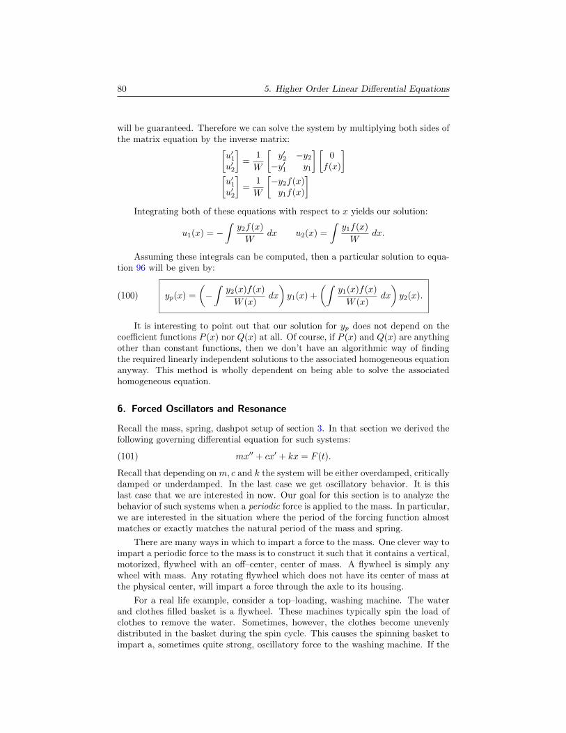
80 5. Higher Order Linear Differential Equations
will be guaranteed. Therefore we can solve the system by multiplying both sides ofthe matrix equation by the inverse matrix:[
u′1u′2
]=
1
W
[y′2 −y2
−y′1 y1
] [0
f(x)
][u′1u′2
]=
1
W
[−y2f(x)y1f(x)
]Integrating both of these equations with respect to x yields our solution:
u1(x) = −∫y2f(x)
Wdx u2(x) =
∫y1f(x)
Wdx.
Assuming these integrals can be computed, then a particular solution to equa-tion 96 will be given by:
(100) yp(x) =
(−∫y2(x)f(x)
W (x)dx
)y1(x) +
(∫y1(x)f(x)
W (x)dx
)y2(x).
It is interesting to point out that our solution for yp does not depend on thecoefficient functions P (x) nor Q(x) at all. Of course, if P (x) and Q(x) are anythingother than constant functions, then we don’t have an algorithmic way of findingthe required linearly independent solutions to the associated homogeneous equationanyway. This method is wholly dependent on being able to solve the associatedhomogeneous equation.
6. Forced Oscillators and Resonance
Recall the mass, spring, dashpot setup of section 3. In that section we derived thefollowing governing differential equation for such systems:
(101) mx′′ + cx′ + kx = F (t).
Recall that depending on m, c and k the system will be either overdamped, criticallydamped or underdamped. In the last case we get oscillatory behavior. It is thislast case that we are interested in now. Our goal for this section is to analyze thebehavior of such systems when a periodic force is applied to the mass. In particular,we are interested in the situation where the period of the forcing function almostmatches or exactly matches the natural period of the mass and spring.
There are many ways in which to impart a force to the mass. One clever way toimpart a periodic force to the mass is to construct it such that it contains a vertical,motorized, flywheel with an off–center, center of mass. A flywheel is simply anywheel with mass. Any rotating flywheel which does not have its center of mass atthe physical center, will impart a force through the axle to its housing.
For a real life example, consider a top–loading, washing machine. The waterand clothes filled basket is a flywheel. These machines typically spin the load ofclothes to remove the water. Sometimes, however, the clothes become unevenlydistributed in the basket during the spin cycle. This causes the spinning basket toimpart a, sometimes quite strong, oscillatory force to the washing machine. If the

6. Forced Oscillators and Resonance 81
basket is unbalanced in the right (wrong?) way, then the back and forth vibrationsof the machine might even knock the washing machine off its base.
Yet another way to force a mass, spring, dashpot system is to drive or force themass via an electromagnet. If the electromagnet has a controllable power source,then it can be used to drive the mass in numerous different ways, i.e. F (t) can takeon numerous shapes.
Undamped Forced Oscillations. If there is no frictional damping, that is ifc = 0, then the associated homogeneous equation for equation 101,
mx′′ + kx = 0,
always results in oscillatory solutions. In this case, we let ω20 = k/m and rewrite
the equation as:x′′ + ω2
0x = 0,
which has characteristic equation, r2 + ω20 = 0, and hence has solution xh(t) =
c1 cosω0t+ c2 sinω0t. Here, ω0 is the natural frequency of the mass spring system,or the frequency at which the system naturally vibrates if pushed out of equilibrium.
When we periodically force the system then we must find a particular solution,xp, in order to assemble the full solution x(t) = xh(t) + xp(t). The method ofundetermined coefficients tells us to make a guess for xp which matches the forcingfunction F (t) and any of its linearly independent derivatives. If the periodic forcingfunction is modeled by:
F (t) = F0 cosωt ω 6= ω0,
then our guess for xp should be: xp = A cosωt + B sinωt, however since the gov-erning equation does not have any first derivatives, B will necessarily be zero, thuswe guess: xp = A cosωt. Plugging this into equation 101, still with c = 0 yields:
−mω2A cosωt+ kA cosωt = F0 cosωt
so
A =F0
k −mω2=
F0/m
ω20 − ω2
.
Thus the solution to equation 101, without damping, i.e. c = 0 is:
x(t) = xh(t) + xp(t)
x(t) = c1 cosω0t+ c2 sinω0t+F0/m
ω20 − ω2
cosωt.
Which with the technique from section 3 can be rewritten:
(102) x(t) = C cos(ω0t− α) +F0/m
ω20 − ω2
cos(ωt).
This is an important result because it helps us to understand the roles of the homo-geneous and particular solutions! In words, this equation says that the response ofa mass spring system to being periodically forced is a superposition of two separateresponses. Recall that C =
√c21 + c22, and similarly α only depends on c1 and c2
which in turn only depend on the initial conditions. Also ω0 is simply a function ofthe properties of the mass and spring, thus the function on the left of (102), i.e. xhrepresents the system’s response to the initial conditions. Notice that the function

82 5. Higher Order Linear Differential Equations
on the right of (102) depends on the driving amplitude (F0), driving frequency (ω)and also m and k, but not at all on the initial conditions. That is, the function onthe right, i.e. xp is the system’s response to being driven or forced.
The homogeneous solution is the system’s response to being disturbed fromequilibrium. The particular solution is the system’s response to being periodicallydriven. The interesting thing is that these two functions are not intertwined insome complicated way. This observation is common to all linear systems, that is, asolution function to any linear system will consist of a superposition of the system’sresponse to intitial conditions and the system’s response to being driven.
Beats. In the previous solution, we assumed that ω 6= ω0. We had to do thisso that xp would be linearly independent from xh. Now we will examine whathappens as ω → ω0, that is if we let the driving frequency (ω) get close to thenatural frequency of oscillation for the mass and spring, (ω0). Clearly, as we letthese two frequencies get close, the amplitude of the particular solution blows up!
limω→ω0
A(ω) = limω→ω0
F0/m
ω20 − ω
=∞.
We will solve for this situation exactly in the next subsection. But what can wesay about the solution when ω ≈ ω0?
This is easiest to analyze if we impose the initial conditions, x(0) = x′(0) = 0on the solution in (102). If we do so, then it is easy to compute the three unknowns:
c1 = − F0
m(ω20 − ω2)
c2 = 0 α = π + tan−1 0 = π.
Recall that cos(ωt− π) = − cos(ωt), hence
xh = C cos(ω0t− π) =F0
m(ω20 − ω2)
cos(ω0t− π) = − F0
m(ω20 − ω2)
cosω0t.
Therefore, the solution to the IVP is:
x(t) =F0
m(ω20 − ω2)
[cosωt− cosω0t]
=F0
m(ω20 − ω2)
[cos(
12 (ω0 + ω)− 1
2 (ω0 − ω))t− cos
(12 (ω0 + ω) + 1
2 (ω0 − ω))t]
=F0
m(ω20 − ω2)
[cos(A−B)− cos(A+B)]
=F0
m(ω20 − ω2)
[2 sinA sinB]
=2F0
m(ω20 − ω2)
[sin 1
2 (ω0 + ω)t sin 12 (ω0 − ω)t
]=
[2F0
m(ω20 − ω2)
sin 12 (ω0 − ω)t
]sin 1
2 (ω0 + ω)t
= A(t) sin 12 (ω0 + ω)t.
Here we have used a trigonometric substitution, so that we could write the solutionas the product of two sine waves. We renamed the expression in large square brack-ets to A(t) which is suggestive of amplitude. Notice that A(t) varies sinusoidally,
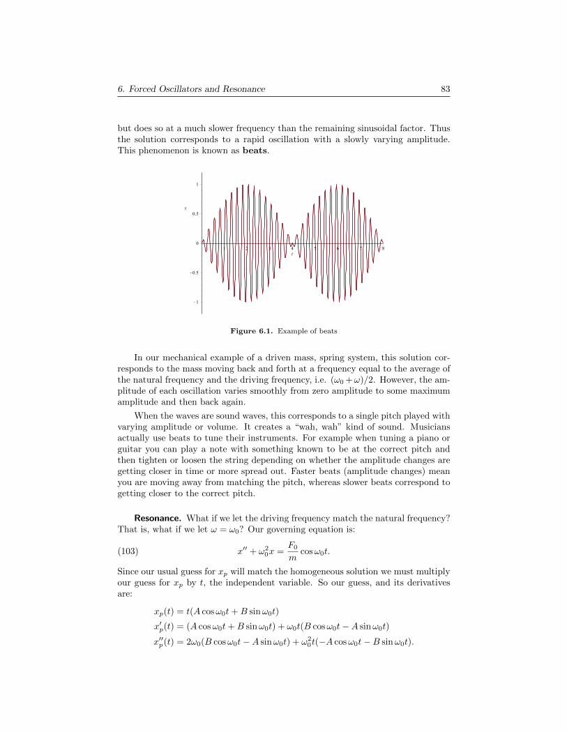
6. Forced Oscillators and Resonance 83
but does so at a much slower frequency than the remaining sinusoidal factor. Thusthe solution corresponds to a rapid oscillation with a slowly varying amplitude.This phenomenon is known as beats.
Figure 6.1. Example of beats
In our mechanical example of a driven mass, spring system, this solution cor-responds to the mass moving back and forth at a frequency equal to the average ofthe natural frequency and the driving frequency, i.e. (ω0 +ω)/2. However, the am-plitude of each oscillation varies smoothly from zero amplitude to some maximumamplitude and then back again.
When the waves are sound waves, this corresponds to a single pitch played withvarying amplitude or volume. It creates a “wah, wah” kind of sound. Musiciansactually use beats to tune their instruments. For example when tuning a piano orguitar you can play a note with something known to be at the correct pitch andthen tighten or loosen the string depending on whether the amplitude changes aregetting closer in time or more spread out. Faster beats (amplitude changes) meanyou are moving away from matching the pitch, whereas slower beats correspond togetting closer to the correct pitch.
Resonance. What if we let the driving frequency match the natural frequency?That is, what if we let ω = ω0? Our governing equation is:
(103) x′′ + ω20x =
F0
mcosω0t.
Since our usual guess for xp will match the homogeneous solution we must multiplyour guess for xp by t, the independent variable. So our guess, and its derivativesare:
xp(t) = t(A cosω0t+B sinω0t)
x′p(t) = (A cosω0t+B sinω0t) + ω0t(B cosω0t−A sinω0t)
x′′p(t) = 2ω0(B cosω0t−A sinω0t) + ω20t(−A cosω0t−B sinω0t).
84 5. Higher Order Linear Differential Equations
Upon plugging these derivatives into equation (103), we get:
x′′p= 2ω0(B cosω0t−A sinω0t) +((((
(((((((
((ω2
0t(−A cosω0t−B sinω0t)
+ω20xp=((((
((((((((
ω20t(A cosω0t+B sinω0t)
F0
mcosω0t= 2ω0(B cosω0t−A sinω0t)
Thus A = 0 and B = F0/2mω0, and our particular solution is:
(104) xp(t) =F0
2mω0t sinω0t.
Figure 6.2. An example of resonance. Functions plotted are:xp(t) = t sin(πt) and the lines x(t) = ±t.
Figure 6.2 shows the graph of xp(t) for the values F0 = ω0 = π,m = 12 . Notice
how the amplitude of oscillation grows linearly without bound, this is resonance.Physically, the mass spring system has a natural frequency at which it changeskinetic energy to potential energy and vice versa. When a driving force matchesthat natural frequency, work is done on the system and hence its total energyincreases.
7. Damped Driven Oscillators


Chapter 6
Laplace Transforms
The Laplace transform is an integral transform that can be used to solve IVPs.Essentially, it transforms a differential equation along with initial values into arational function. Whereupon the task will be to rewrite the rational function intoits partial fractions decomposition. After rewriting the rational function in thissimplified form, you can then perform the inverse Laplace transform to find thesolution.
Just as with all other solution methods for higher–order, linear, differentialequations, the Laplace transform method reduces the problem to an algebraic one,in this case a partial fractions decomposition problem.
Unfortunately, the Laplace transform method typically requires more work, orcomputation than the previous methods of undetermined coefficients and variationof parameters. But the Laplace method is more powerful. It will allow us to solveequations with more complicated forcing functions than before. It is especiallyuseful for analyzing electric circuits where the power is periodically switched onand off.
1. The Laplace Transform
Definition 6.1. If a function f(t) is defined for t ≥ 0, then its Laplace transformis denoted F (s) and defined by the integral:
F (s) = L f(t) =
∫ ∞0
e−stf(t) dt
for all values of s for which the improper integral converges.
Notice that the last sentence of the above definition reminds us that improperintegrals do not necessarily converge, i.e. equal a finite number. Thus when comput-ing Laplace transforms of functions, we must be careful to state any assumptionson s which we make to ensure convergence. Another way to think of this is that the
87

88 6. Laplace Transforms
domain of a transformed function, say F (s) is almost never the whole real numberline.
Example 6.2. L k =k
s
Recall that both the integral and the limit operator are linear, so we can pullconstants outside of these operations.
L k =
∫ ∞0
e−stk dt
= k limb→∞
∫ b
0
e−st dt
= k limb→∞
[−1
se−st
]t=bt=0
= k limb→∞
*0
−1
se−sb +
1
s
s > 0
=k
sfor s > 0.
4
Example 6.3. Leat
=1
s− a
Leat
=
∫ ∞0
e−steat dt
=
∫ ∞0
e(−s+a)t dt let u = (−s+ a)t du = −(s− a)dt
=
∫ ∞0
−eu
s− adu
= limb→∞
[−e−(s−a)t
s− a
]t=bt=0
= limb→∞
*0
−e−(s−a)b
s− a+
1
s− a
s > a
=1
s− afor s > a.
4
Notice that the integral in the previous example diverges if s ≤ a, thus we mustrestrict the domain of the transformed function to s > a.
Example 6.4. L t =1
s2
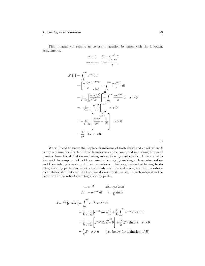
1. The Laplace Transform 89
This integral will require us to use integration by parts with the followingassignments,
u = t dv = e−st dt
du = dt v =−e−st
s.
L t =
∫ ∞0
e−stt dt
=
[−te−st
s
]t=∞t=0
−∫ ∞
0
−e−st
sdt
= limb→∞
*0[
−be−sb
s
]−∫ ∞
0
−e−st
sdt s > 0
= − limb→∞
[e−st
s2
]t=bt=0
s > 0
= − limb→∞
0
e−sb
s2− 1
s2
s > 0
=1
s2for s > 0.
4
We will need to know the Laplace transforms of both sin kt and cos kt where kis any real number. Each of these transforms can be computed in a straightforwardmanner from the definition and using integration by parts twice. However, it isless work to compute both of them simultaneously by making a clever observationand then solving a system of linear equations. This way, instead of having to dointegration by parts four times we will only need to do it twice, and it illustrates anice relationship between the two transforms. First, we set up each integral in thedefinition to be solved via integration by parts.
u= e−st dv= cos kt dt
du= −se−st dt v=1
ksin kt
A = L cos kt =
∫ ∞0
e−st cos kt dt
=1
klimb→∞
[e−st sin kt
]b0
+s
k
∫ ∞0
e−st sin kt dt
=1
klimb→∞
[
:0e−sb sin k − 0
]+s
kL sin kt s > 0
=s
kB s > 0 (see below for definition of B)

90 6. Laplace Transforms
u= e−st dv= sin kt dt
du= −se−st dt v= −1
kcos kt
B = L sin kt =
∫ ∞0
e−st sin kt dt
= −1
klimb→∞
[e−st cos kt
]b0− s
k
∫ ∞0
e−st cos kt dt
= −1
klimb→∞
[
:0e−sb cos kb− 1
]− s
kL cos kt s > 0
=1
k− s
kA s > 0
Thus we have the following system:
A− s
kB = 0
s
kA+B =
1
k,
which upon solving and recalling A = L cos kt and B = L sin kt yields:
L cos kt= s
s2 + k2
L sin kt= k
s2 + k2
Theorem 6.5. Linearity of the Laplace Transform
If a, b ∈ R are constants, and f and g are any two functions whose Laplacetransforms exist, then:
(105) L af(t) + bg(t) = aL f(t)+ bL g(t) = aF (s) + bG(s),
for all s such that the Laplace transforms of both functions f and g exist.
Proof. Recall that both the integral and the limit operators are linear, thus:
L af(t) + bg(t) =
∫ ∞0
e−st[af(t) + b g(t)] dt
= limc→∞
∫ c
0
e−st[af(t) + b g(t)] dt
= a limc→∞
∫ c
0
e−stf(t) dt+ b limc→∞
∫ c
0
e−stg(t) dt
= aL f(t)+ bL g(t)= aF (s) + bG(s)

1. The Laplace Transform 91
Example 6.6. L cosh kt =s
s2 − k2
L cosh kt = L
ekt + e−kt
2
=
1
2
[Lekt
+ Le−kt
]=
1
2
[1
s− k+
1
s+ k
]=
1
2
[s+ k + s− ks2 − k2
]=
s
s2 − k2
4
Example 6.7. L sinh kt =k
s2 − k2
L sinh kt = L
ekt − e−kt
2
=
1
2
[Lekt−L
e−kt
]=
1
2
[1
s− k− 1
s+ k
]=
1
2
[s+ k − s+ k
s2 − k2
]=
k
s2 − k2
4
Theorem 6.8. Translation on the s-Axis
If the Laplace transform of y(t) exists for s > b, then
Leaty(t)
= Y (s− a) for s > a+ b.
Proof.
Leaty(t)
=
∫ ∞0
e−steaty(t) dt
=
∫ ∞0
e−(s−a)ty(t) dt
= Y (s− a)
We have computed Laplace transforms of a few different functions, but thequestion naturally arises, can we compute a Laplace transform for every function?
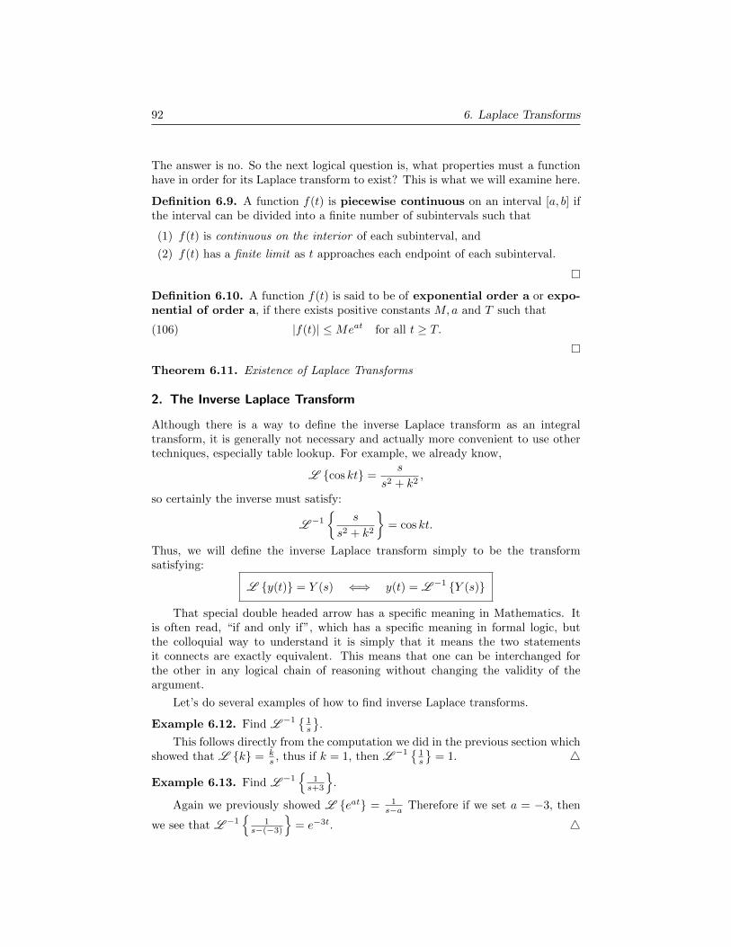
92 6. Laplace Transforms
The answer is no. So the next logical question is, what properties must a functionhave in order for its Laplace transform to exist? This is what we will examine here.
Definition 6.9. A function f(t) is piecewise continuous on an interval [a, b] ifthe interval can be divided into a finite number of subintervals such that
(1) f(t) is continuous on the interior of each subinterval, and
(2) f(t) has a finite limit as t approaches each endpoint of each subinterval.
Definition 6.10. A function f(t) is said to be of exponential order a or expo-nential of order a, if there exists positive constants M,a and T such that
(106) |f(t)| ≤Meat for all t ≥ T.
Theorem 6.11. Existence of Laplace Transforms
2. The Inverse Laplace Transform
Although there is a way to define the inverse Laplace transform as an integraltransform, it is generally not necessary and actually more convenient to use othertechniques, especially table lookup. For example, we already know,
L cos kt =s
s2 + k2,
so certainly the inverse must satisfy:
L −1
s
s2 + k2
= cos kt.
Thus, we will define the inverse Laplace transform simply to be the transformsatisfying:
L y(t) = Y (s) ⇐⇒ y(t) = L −1 Y (s)
That special double headed arrow has a specific meaning in Mathematics. Itis often read, “if and only if”, which has a specific meaning in formal logic, butthe colloquial way to understand it is simply that it means the two statementsit connects are exactly equivalent. This means that one can be interchanged forthe other in any logical chain of reasoning without changing the validity of theargument.
Let’s do several examples of how to find inverse Laplace transforms.
Example 6.12. Find L −1
1s
.
This follows directly from the computation we did in the previous section whichshowed that L k = k
s , thus if k = 1, then L −1
1s
= 1. 4
Example 6.13. Find L −1
1s+3
.
Again we previously showed L eat = 1s−a Therefore if we set a = −3, then
we see that L −1
1s−(−3)
= e−3t. 4

2. The Inverse Laplace Transform 93
Example 6.14. Find L −1
ss2+5
.
This matches the formula L cos kt = ss2+k2 with k =
√5 so that k2 = 5,
thus L −1
ss2+5
= cos
√5t. 4
Example 6.15. Find L −1s+1s2−4
.
After a simple rewrite, we see that the transforms of cosh kt and sinh kt apply.
L −1
s+ 1
s2 − 4
= L −1
s
s2 − 4
+ L −1
1
s2 − 4
= cosh 2t+ L −1
1
2
(2
s2 − 4
)= cosh 2t+
1
2L −1
2
s2 − 4
= cosh 2t+
1
2sinh 2t
4
Example 6.16. Find L −1
s(s−2)2+9
.
This example will rely on the translation on the s-axis theorem, or theorem 6.8from the previous section, which summarized says:
Leaty(t)
= Y (s− a)
eaty(t) = L −1 Y (s− a)
L −1
s
(s− 2)2 + 9
= L −1
s− 2 + 2
(s− 2)2 + 9
= L −1
(s− 2)
(s− 2)2 + 9
+ L −1
2
(s− 2)2 + 9
= e2t cos 3t+ L −1
2
3
(3
(s− 2)2 + 9
)= e2t cos 3t+
2
3L −1
(3
(s− 2)2 + 9
)= e2t cos 3t+
2
3e2t sin 3t
4
Example 6.17. Find L −1
1s2+4s+8
.
First we complete the square in the denominator.
1
s2 + 4s+ 8=
1
(s2 + 4s+ 4)− 4 + 8=
1
(s+ 2)2 + 4
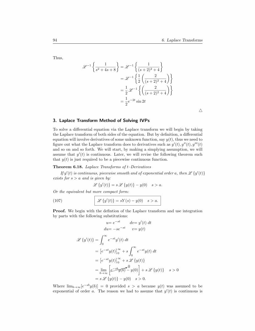
94 6. Laplace Transforms
Thus,
L −1
1
s2 + 4s+ 8
= L −1
1
(s+ 2)2 + 4
= L −1
1
2
(2
(s+ 2)2 + 4
)=
1
2L −1
(2
(s+ 2)2 + 4
)=
1
2e−2t sin 2t
4
3. Laplace Transform Method of Solving IVPs
To solve a differential equation via the Laplace transform we will begin by takingthe Laplace transform of both sides of the equation. But by definition, a differentialequation will involve derivatives of some unknown function, say y(t), thus we need tofigure out what the Laplace transform does to derivatives such as y′(t), y′′(t), y′′′(t)and so on and so forth. We will start, by making a simplying assumption, we willassume that y′(t) is continuous. Later, we will revise the following theorem suchthat y(t) is just required to be a piecewise continuous function.
Theorem 6.18. Laplace Transforms of t–Derivatives
If y′(t) is continuous, piecewise smooth and of exponential order a, then L y′(t)exists for s > a and is given by:
L y′(t) = sL y(t) − y(0) s > a.
Or the equivalent but more compact form:
(107) L y′(t) = sY (s)− y(0) s > a.
Proof. We begin with the defintion of the Laplace transform and use integrationby parts with the following substitutions:
u= e−st dv= y′(t) dt
du= −se−st v= y(t)
L y′(t) =
∫ ∞0
e−sty′(t) dt
=[e−sty(t)
]∞0
+ s
∫ ∞0
e−sty(t) dt
=[e−sty(t)
]∞0
+ sL y(t)
= limb→∞
[
:0e−sby(b)− y(0)
]+ sL y(t) s > 0
= sL y(t) − y(0) s > 0.
Where limb→∞[e−sby(b)] = 0 provided s > a because y(t) was assumed to beexponential of order a. The reason we had to assume that y′(t) is continuous is
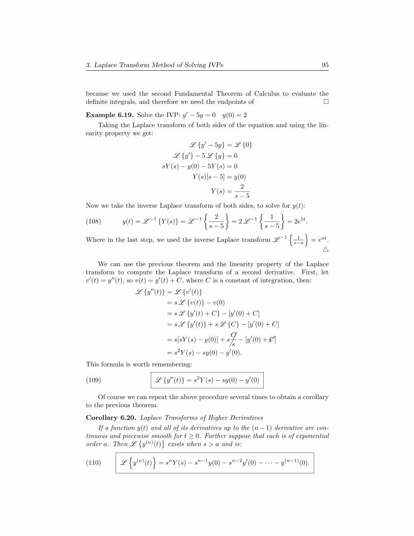
3. Laplace Transform Method of Solving IVPs 95
because we used the second Fundamental Theorem of Calculus to evaluate thedefinite integrals, and therefore we need the endpoints of
Example 6.19. Solve the IVP: y′ − 5y = 0 y(0) = 2
Taking the Laplace transform of both sides of the equation and using the lin-earity property we get:
L y′ − 5y = L 0L y′ − 5 L y = 0
sY (s)− y(0)− 5Y (s) = 0
Y (s)[s− 5] = y(0)
Y (s) =2
s− 5
Now we take the inverse Laplace transform of both sides, to solve for y(t):
(108) y(t) = L −1 Y (s) = L −1
2
s− 5
= 2 L −1
1
s− 5
= 2e5t.
Where in the last step, we used the inverse Laplace transform L −1
1s−a
= eat.
4
We can use the previous theorem and the linearity property of the Laplacetransform to compute the Laplace transform of a second derivative. First, letv′(t) = y′′(t), so v(t) = y′(t) + C, where C is a constant of integration, then:
L y′′(t) = L v′(t)= sL v(t) − v(0)
= sL y′(t) + C − [y′(0) + C]
= sL y′(t)+ sL C − [y′(0) + C]
= s[sY (s)− y(0)] + sC
s− [y′(0) +C]
= s2Y (s)− sy(0)− y′(0).
This formula is worth remembering:
(109) L y′′(t) = s2Y (s)− sy(0)− y′(0)
Of course we can repeat the above procedure several times to obtain a corollaryto the previous theorem.
Corollary 6.20. Laplace Transforms of Higher Derivatives
If a function y(t) and all of its derivatives up to the (n− 1) derivative are con-tinuous and piecewise smooth for t ≥ 0. Further suppose that each is of exponentialorder a. Then L
y(n)(t)
exists when s > a and is:
(110) Ly(n)(t)
= snY (s)− sn−1y(0)− sn−2y′(0)− · · · − y(n−1)(0).

96 6. Laplace Transforms
If you examine all three results for Laplace transforms of derivatives in thissection, you will notice that if the graph of a function passes through the origin,that is if y(0) = 0, and assuming y(t) meets the hypotheses of theorem 6.18, thendifferentiating in the t domain corresponds to multiplication by s in the s domain,or L y′(t) = sY (s). We can sometimes exploit this to our advantage as the nextexample illustrates.
Example 6.21. Lteat
=
1
(s− a)2
Let y(t) = teat, then y(0) = 0, thus
L y′(t) = Leat + teat
= L
eat
+ Lateat
=
1
s− a+ aY (s)
Now using theorem 6.18, y(0) = 0 and the result just calculated, we get:
sY (s) =1
s− a+ aY (s)
(s− a)Y (s) =1
s− a
Y (s) =1
(s− a)2
4
The previous example exploited the fact that if y(0) = 0, then the Laplacetransform of the derivative of y(t) is obtained simply by multiplying the Laplacetransform of y(t) by s. In symbols this can be concisely stated:
L y′(t) = sY (s) y(0) = 0.
Thus multiplying by s in the s domain corresponds to differentiating with respectto t in the t domain, under the precise circumstance y(0) = 0. It is natural towonder whether the inverse operation of multiplying by s, namely dividing by scorresponds to the inverse of the derivative namely integrating in the t domain.And it does!
Theorem 6.22. Laplace Transforms of Integrals
If y(t) is a piecewise continuous function and is of exponential order a fort ≥ T , then:
L
∫ t
0
y(τ) dτ
=
1
sL y(t) =
1
sY (s) s > a.
The inverse transform way to interpret the previous theorem is simply:∫ t
0
y(τ) dτ = L −1
1
sY (s)
.

3. Laplace Transform Method of Solving IVPs 97
Example 6.23. Use theorem 6.22 to find L −1
1s(s2+1)
.
L −1
1
s(s2 + 1)
=
∫ t
0
L −1
1
s2 + 1
dτ
=
∫ t
0
sin τ dτ
= [− cos τ ]t0
= − cos t−− cos 0
= 1− cos t
4
Example 6.24. Solve the following IVP: y′ + y = sin t y(0) = 1
First we take the Laplace transform of both sides of the equation.
L y′(t) + y(t) = L sin t
L y′(t)+ L y(t) =1
s2 + 1by theorem 6.5
sY (s)− y(0) + Y (s) =1
s2 + 1by theorem 6.18
sY (s)− 1 + Y (s) =1
s2 + 1applied initial condition y(0) = 1
(s+ 1)Y (s) =1
s2 + 1+ 1
Y (s) =1
(s+ 1)(s2 + 1)+
1
s+ 1
Now if we apply the inverse Laplace transform to both sides of the last equation,we will get y(t) on the left, which is the solution function we seek! But in order tocompute the inverse Laplace transform of the right hand side, we need to recognizeit as the Laplace transform of some function or sum of functions. Since 1
s+1 =1
s−(−1) the term on the right has inverse Laplace transform e−t, (recall L eat =1s−a ). But the term on the left has no obvious inverse Laplace transform. Sincethe denominator is a product of irreducible factors, we can do a partial fractionsdecomposition. That is,
1
(s+ 1)(s2 + 1)=
A
s+ 1+Bs+ C
s2 + 1
1
(s+ 1)(s2 + 1)=A(s2 + 1) + (Bs+ C)(s+ 1)
(s+ 1)(s2 + 1)
Equating just the numerators yields,
1 = A(s2 + 1) + (Bs+ C)(s+ 1)
1 = As2 +A+Bs2 +Bs+ Cs+ C
1 = (A+B)s2 + (B + C)s+ (A+ C)

98 6. Laplace Transforms
By equating the coefficients of powers of s on both sides we get three equations inthe three unknowns, A,B and C.
A +B = 0
B+C= 0
A +C= 1
Which you can check by inspection has solution A = 1/2, B = −1/2, C = 1/2.Thus,
Y (s) =12
s+ 1+− 1
2s+ 12
s2 + 1+
1
s+ 1
Y (s) =1
2
(1
s+ 1
)− 1
2
(s− 1
s2 + 1
)+
1
s+ 1
Y (s) =3
2
(1
s+ 1
)− 1
2
(s
s2 + 1
)+
1
2
(1
s2 + 1
)y(t) =
3
2L −1
1
s+ 1
− 1
2L −1
s
s2 + 1
+
1
2L −1
1
s2 + 1
y(t) =
3
2e−t − 1
2cos t+
1
2sin t
4
Example 6.25. Solve the following IVP: y′′(t)+y(t) = cos 2t y(0) = 0, y′(0) = 1.
We proceed by taking the Laplace transform of both sides of the equation anduse the linearity property of the Laplace transform (theorem 6.5).
L y′′(t) + y(t) = L cos 2t
L y′′(t)+ L y(t) =s
s2 + 4
s2Y (s)− sy(0)− y′(0) + Y (s) =s
s2 + 4
s2Y (s)− 1 + Y (s) =s
s2 + 4
(s2 + 1)Y (s)− 1 =s
s2 + 4
(s2 + 1)Y (s) =s
s2 + 4+s2 + 4
s2 + 4
Y (s) =s2 + s+ 4
(s2 + 1)(s2 + 4)
Now we must do a partial fractions decomposition of this rational function.
s2 + s+ 4
(s2 + 1)(s2 + 4)=As+B
s2 + 1+Cs+D
s2 + 4
s2 + s+ 4 = (As+B)(s2 + 4) + (Cs+D)(s2 + 1)
s2 + s+ 4 = (As3 + 4As+Bs2 + 4B) + (Cs3 + Cs+Ds2 +D)
s2 + s+ 4 = (A+ C)s3 + (B +D)s2 + (4A+ C)s+ (4B +D)

3. Laplace Transform Method of Solving IVPs 99
1 0 1 00 1 0 14 0 1 00 4 0 1
ABCD
=
0114
=⇒
ABCD
=
1/31−1/3
0
Y (s) =
1
3
s
s2 + 1− 1
3
s
s2 + 4+
1
s2 + 1Finally, we apply the inverse Laplace transform to both sides to yield:
y(t) =1
3cos t+ sin t− 1
3cos 2t.
4
3.1. Electrical Circuits. A series electrical RLC circuit is analogous to a mass,spring, dashpot system. The resistor with resistance R measured in ohms (ω)is like the dashpot because it resists the flow of electrons. The capacitor withcapacitance C measured in Farads is like the spring, because it converts electronflow into potential energy similar to how a spring converts kinetic energy intopotential energy. Finally, the inductor with inductance L measured in Henries islike the mass, because it resists the flow of electrons initially, but once the currentreaches its maximum, the inductor also resists any decrease in current.
If we sit at some point in the circuit and count the amount of charge whichpasses as a function of time, and denote this by q(t), then Kirchoff’s Current Lawand Kirchoff’s Voltage Law yield the following equation for a series RLC circuit.
(111) Lq′′ +Rq′ +1
Cq = e(t)
By definition the current i(t) is the time rate of change of charge q(t), thus:
i(t) =dq
dt= q′(t) =⇒ q(t) =
∫ t
0
i(τ) dτ.
This allows us to rewrite equation 111, in the following way.
(112) Li′ +Ri+1
C
∫ t
0
i(τ) dτ = e(t)
V0 sin(ωt)
Is
C
L
R
(a) Series RLC circuit
V0 sin(ωt)
Ip
C
IC
L
IL
R
IR
(b) Parallel RLC Circuit
Figure 3.1. RLC Circuits: a Series RLC configuration. b Parallel RLC configuration
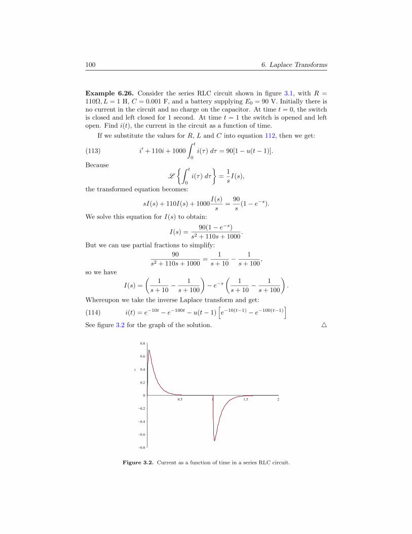
100 6. Laplace Transforms
Example 6.26. Consider the series RLC circuit shown in figure 3.1, with R =110Ω, L = 1 H, C = 0.001 F, and a battery supplying E0 = 90 V. Initially there isno current in the circuit and no charge on the capacitor. At time t = 0, the switchis closed and left closed for 1 second. At time t = 1 the switch is opened and leftopen. Find i(t), the current in the circuit as a function of time.
If we substitute the values for R, L and C into equation 112, then we get:
(113) i′ + 110i+ 1000
∫ t
0
i(τ) dτ = 90[1− u(t− 1)].
Because
L
∫ t
0
i(τ) dτ
=
1
sI(s),
the transformed equation becomes:
sI(s) + 110I(s) + 1000I(s)
s=
90
s(1− e−s).
We solve this equation for I(s) to obtain:
I(s) =90(1− e−s)
s2 + 110s+ 1000.
But we can use partial fractions to simplify:
90
s2 + 110s+ 1000=
1
s+ 10− 1
s+ 100,
so we have
I(s) =
(1
s+ 10− 1
s+ 100
)− e−s
(1
s+ 10− 1
s+ 100
).
Whereupon we take the inverse Laplace transform and get:
(114) i(t) = e−10t − e−100t − u(t− 1)[e−10(t−1) − e−100(t−1)
]See figure 3.2 for the graph of the solution. 4
Figure 3.2. Current as a function of time in a series RLC circuit.

4. Switching 101
4. Switching
Definition 6.27. The unit step function corresponds to an “on switch”. It isdefined by
(115) ua(t) = u(t− a) =
0 t < a
1 t > a
−1 1 2 3 4t
−1
1
2
u(t− 2)
0 −1 1 2 3 4t
−1
1
2
2u(t− 1)
0
Figure 4.1. Examples of step functions
This function acts like a switch for turning something on. For example, if youwant to turn on the function f(t) = t2 at time t = 1, then you could multiply f(t)by u(t− 1). But more likely, you would probably like the function f(t) = t2 to actas if time begins at time t = 1. This is accomplished by first shifting the input tof , for example f(t− 1), and then multiplying by u(t− 1).
−1 1 2 3 4t
−1
1
2
t2 · u(t− 1)
0 −1 1 2 3 4t
−1
1
2
(t− 1)2 · u(t− 1)
0
Figure 4.2. Switching on t2 versus (t− 1)2 via the step function u(t− 1)
We can also repurpose the unit step function as a way to turn things off.
Lemma 6.28. The unit step function, u(t − a), changes to a “switch off at timea” function when its input is multiplied by -1.
u(a− t) =
1 t < a
0 t > a
Proof. The unit step function is defined to be
u(t− a) =
0 t < a
1 t > a⇐⇒ u(t− a) =
0 t− a < 0
1 t− a > 0
102 6. Laplace Transforms
Multiplying the input by (-1) requires us to flip the inequalities in the above defi-nition yielding:
u(a− t) =
0 a− t > 0
1 a− t < 0⇐⇒ u(a− t) =
0 t > a
1 t < a
5. Convolution
Definition 6.29. Let f(t), g(t) be piecewise continuous functions for t ≥ 0. Theconvolution of f with g denoted by f ∗ g is defined by
(116) (f ∗ g)(t) =
∫ t
0
f(τ)g(t− τ) dτ.
Theorem 6.30 (Convolution is Commutative). Let f(t) and g(t) be piecewise con-tinuous on [0,∞), then
f ∗ g = g ∗ f.
Proof. We can rewrite the convolution integral using the following substitution:
v = t− τ ⇐⇒ τ = t− v =⇒ dτ = −dv.
f ∗ g =
∫ t
0
f(τ)g(t− τ) dτ
=
∫ τ=t
τ=0
f(t− v)g(v) (−dv)
When τ = 0, v = t− 0 = t and when τ = t, v = t− t = 0.
= −∫ 0
t
f(t− v)g(v) dv
=
∫ t
0
g(v)f(t− v) dv
= g ∗ f
Theorem 6.31 (The Convolution Theorem). If f(t) and g(t) are piecewise con-tinuous and of exponential order c, then the Laplace transform of f ∗ g exists fors > c and is given by
(117) L f(t) ∗ g(t) = F (s) ·G(s),
or equivalently,
(118) L −1 F (s) ·G(s) = f(t) ∗ g(t).

5. Convolution 103
Proof. We start with the definitions of the Laplace transform and of convolutionand get the iterated integral:
L f(t) ∗ g(t) =
∫ ∞0
e−st[∫ t
0
f(τ)g(t− τ) dτ
]dt.
Next, notice that we can change the bounds of integration on the second integral ifwe multiply the integrand by the unit step function u(t−τ), where τ is the variableand t is the switch off time (see lemma 6.28):
L f(t) ∗ g(t) =
∫ ∞0
e−st[∫ ∞
0
f(τ)u(t− τ)g(t− τ) dτ
]dt,
Reversing the order of integration gives
L f(t) ∗ g(t) =
∫ ∞0
f(τ)
[∫ ∞0
e−stu(t− τ)g(t− τ) dt
]dτ,
The integral in square brackets can be rewritten by theorem ?? as e−sτG(s), giving
L f(t) ∗ g(t) =
∫ ∞0
f(τ)e−sτG(s)dτ = G(s)
∫ ∞0
e−sτf(τ)dτ = F (s) ·G(s).
Definition 6.32. The transfer function, H(s), of a linear system is the ratio ofthe Laplace transform of the output function to the Laplace transform of the inputfunction when all initial conditions are zero.
H(s) =X(s)
F (s).
Definition 6.33. The function h(t) = L −1 H(s), is called the impulse responsefunction. It is called this because it is the system’s response to receiving a unitimpulse of force at time zero.
The impulse response function is also the unique solution to the following un-driven (homogeneous) IVP:
mx′′ + cx′ + kx = 0; x(0) = 0, x′(0) =1
m.
m
s2X(s)− s*0
x(0)−*
1m
x′(0)
+ c
[sX(s)−*
0x(0)
]+ kX(s) = 0
m
[s2X(s)− 1
m
]+ csX(s) + kX(s) = 0
(ms2 + cs+ k)X(s) = 1
X(s) =1
ms2 + cs+ k
The importance of the impulse response function, h(t) is that once we knowhow the system responds to a unit impulse, then we can convolve that response

104 6. Laplace Transforms
with any forcing function, f(t), to determine the system’s response to being drivenin any manner.

Chapter 7
Eigenvalues and Eigenvectors
In the next chapter, we will see how some problems are more naturally modeledvia a system or collection of differential equations. We will solve these systems ofequations by first transforming the system into a matrix equation, then finding theeigenvalues and eigenvectors which belong to that matrix and finally constructinga solution from those eigenvalues and eigenvectors.
We will also develop a simple algorithm to transform a single, higher order,linear, differential equation into a system of first order equations. For example, athird order, linear equation will transform into a system of three first order, linearequations. In general, an n–th order, linear differential equation can always betransformed into a system of n, first order, linear, differential equations. This sys-tem can be solved via eigenvalues and eigenvectors and then the reverse algorithmtranslates the matrix solution back to the context of the original problem.
Thus the theory behind eigenvalues and eigenvectors has direct applicationto solving differential equations, but it actually does much more! In chapter 9,eigenvalues and eigenvectors will allow us to understand differential equations froma geometric perspective. Perhaps most surprising is that although the theory arisesfrom a study of linear systems, it will also allow us to qualitatively understandnonlinear systems!
A very large number of problems in science and engineering eventually distilldown to “the eigenvalue problem”. From web search to petroleum exploration toarchiving fingerprints to modeling the human heart, the variety of applications ofthis theory are so myriad that it would be a daunting task to try to enumeratethem.
1. Introduction to Eigenvalues and Eigenvectors
Let’s start with a square n×n matrix. Recall that such a matrix can be thought ofas a function which maps Rn to itself. Unfortunately, even for the simplest case ofa 2× 2 matrix, we can’t graph this function like we did the functions in Calculus.
105

106 7. Eigenvalues and Eigenvectors
This is because the graph would have to exist in a four dimensional space. Thegraph of a 3× 3 matrix requires a six dimensional space, and in general the graphof an n × n matrix requires a 2n dimensional space. Since direct visualization ofmatrix mappings is not possible, we must get clever!
A mapping takes an input and maps it to an output. That is, it changesone thing into another. But sometimes a mapping maps an input back to itself.Matrices map input vectors to output vectors. Some matrices have special vectorswhich get mapped exactly back to themselves, but usually this is not the case.However, many matrices do map certain vectors to scalar multiples of themselves.This situation is very common. A vector ~v which gets mapped to a scalar multipleof itself under the matrix A is called an eigenvector of A. In symbols we write:
(119) A~v = λ~v.
In the above equation, the symbol, λ (pronounced “lambda”), is the scalarmultiplier of ~v. We call λ the eigenvalue associated with the eigenvector, ~v. Aneigenvalue can be any real number, even zero. However, since ~v = ~0 is always asolution to equation (119) we will disallow the zero vector from being called aneigenvector. In other words we are only interested in the nontrival, i.e. non zero–vector solutions.
Example 7.1. Consider the matrix A =
[3 −1−1 3
].
The vector ~v1 =
[11
]is an eigenvector of A with eigenvalue λ1 = 2, because:
A~v1 =
[3 −1−1 3
] [11
]=
[22
]= 2
[11
]= λ1~v1.
The vector ~v2 =
[−1
1
]is an eigenvector of A with eigenvalue λ2 = 4, because:
A~v2 =
[3 −1−1 3
] [−1
1
]=
[−4
4
]= 4
[−1
1
]= λ2~v2.
Any scalar multiple of an eigenvector is again an eigenvector corresponding to thesame eigenvalue. For example,
1
2~v1 =
1
2
[11
]=
[1/21/2
]is an eigenvector because:
A(1/2)~v1 =
[3 −1−1 3
] [1/21/2
]=
[11
]= 2
[1/21/2
]= λ1(1/2)~v1.
4
The fact that a scalar multiple of an eigenvector is again an eigenvector cor-responding to the same eigenvalue is simply a consequence of the fact that scalar

2. Algorithm for Computing Eigenvalues and Eigenvectors 107
multiplication of matrices and hence vectors commutes. That is, if λ,~v form aneigenvalue, eigenvector pair for the matrix A, and c is any scalar, then
A~v = λ~v
cA~v = cλ~v
A(c~v) = λ(c~v).
2. Algorithm for Computing Eigenvalues and Eigenvectors
Given a square n × n matrix, A, how can we compute its eigenvalues and eigen-vectors? We need to solve equation (119): A~v = λ~v, but this equation has twounknowns: λ which is a scalar and ~v which is a vector. The trick is to transformthis equation into a homogeneous equation and use our knowledge of linear systems.First we rewrite equation (119) as
A~v − λ~v = ~0.
Notice that both terms on the left hand side involve ~v so let’s factor ~v out:
(A− λ)~v = ~0.
The last equation is problematic because it makes no sense to subtract the scalarλ from the matrix A! However there is an easy fix. Recall that the identity matrixI is called the identity exactly because it maps all vectors to themselves. That is,I~v = ~v for all vectors ~v. Thus we can rewrite the previous two equations as follows:
A~v − λI~v = ~0
(A− λI)~v = ~0.(120)
Now the quantity in parentheses makes sense because λI is an n×n matrix just likeA. This last linear system is homogeneous and thus at least has solution ~v = ~0, butby definition we disallow the zero vector from being an eigenvector simply becauseit is an eigenvector for every matrix, and thus provides no information about A.Instead we are interested in the nonzero vectors which solve equation (120).


Chapter 8
Systems of DifferentialEquations
1. First Order Systems
A system of differential equations is simply a set or collection of DEs. A first ordersystem is simply a set of first order, linear DEs. For example,
dx
dt= 3x− y
dy
dt=−x+ 3y
Solving a first order system is usually not as simple as solving two individual firstorder DEs. Notice that in the system above, we cannot solve for x(t) withoutalso simultaneously solving for y(t). This is because dx/dt depends on two varyingquantities. When at least one of the equations in a system depends on more thanone variable we say the system is coupled.
This system can be rewritten as an equivalent matrix equation:
(121)
[x′
y′
]=
[3 −1−1 3
] [xy
]which in turn can be written in the very compact form:
(122) ~x ′ = A~x
where ~x ′ =
[x′
y′
], A =
[3 −1−1 3
]and ~x =
[xy
].
When we wish to emphasize the fact that both ~x ′ and ~x are vectors of functionsand not just constant vectors, we will write equation (122) in the following way:
(122) ~x ′(t) = A~x(t)
109

110 8. Systems of Differential Equations
Our method of solution will closely parallel that of chapter 5, where we guessedwhat form the solution might take and then plugged that guess into the governingDE to determine constaints on our guess.
For a system of n first order equations, we guess that solutions have the form
(123) ~x(t) = ~veλt
where λ is a scalar (possibly complex), and where ~v is an n–dimensional vector ofscalars (again, possibly complex). To be clear we are assuming that ~x(t) can bewritten in the following way:
~x(t) = ~veλtx1(t)x2(t)
...xn(t)
=
v1
v2
...vn
eλtx1(t)x2(t)
...xn(t)
=
v1e
λt
v2eλt
...vne
λt
If the vector–valued function ~x(t) = ~veλt is to be a solution to equation (122) thenits derivative must equal A~x. Computing its derivative yields:
~x ′(t) =d
dt
(~veλt
)x′1(t)x′2(t)
...x′n(t)
=
λv1e
λt
λv2eλt
...λvne
λt
x′1(t)x′2(t)
...x′n(t)
= λ
v1e
λt
v2eλt
...vne
λt
~x ′(t) = λ~veλt
~x ′(t) = λ~x(t)(124)
Equating the right hand sides of equation (122) and equation (124) gives:
(125) A~x(t) = λ~x(t)
which is the eigenvalue–eigenvector equation from chapter 7. The only differencebeing that now the eigenvector is a vector of functions of t as opposed to justscalars. Since the solutions of equation (125) are actually vector–valued functionswe will usually refer to them as eigenfunctions rather than eigenvectors, howeverit is common to just say eigenvector as well.

1. First Order Systems 111
Guessing that our solution has the form ~x(t) = ~veλt forces our solution tosatisfy equation (125). Thus, solving a system of first order DEs is equivalentto computing the eigenvalues and eigenvectors of the matrix A which encodes thesalient features of the system. We know from chapter 7 that if A is an n×n matrix,then it will have n linearly independent eigenvectors. The set of eigenpairs,
λ1, ~v1, λ2, ~v2, . . . , λn, ~vn
allow us to form a basis of eigenfunctions,~x1(t) = ~v1e
λ1t, ~x2(t) = ~v2eλ2t, . . . , ~xn(t) = ~vne
λnt
which span the solution space of equation (125). Since the eigenfunctions form abasis for the solution space, we can express the solution ~x(t) as a linear combinationof them,
~x(t) = c1~x1(t) + c2~x2(t) + · · ·+ cn~xn(t)(126)
~x(t) = c1~v1eλ1t + c2~v2e
λ2t + · · ·+ cn~vneλnt
Example 8.1. Let’s solve the example system from the beginning of the chapter,which we reproduce here, but let’s also add initial values. Since we have two firstorder DEs, we need two initial values.
(121)
[x′
y′
]=
[3 −1−1 3
] [xy
]x(0) = 6, y(0) = 0
For convenience we will refer to the coefficient matrix above as A. Computing theeigenvalues of matrix A yields two distinct eigenvalues λ1 = 2 and λ2 = 4, because
|A− λI| =∣∣∣∣3− λ −1−1 3− λ
∣∣∣∣ = (3− λ)2 − 1
= (λ− 3)2 − 1
= λ2 − 6λ+ 8
= (λ− 2)(λ− 4) = 0.
Solving the eigenvector equation, (A− λI)~v = ~0 for each eigenvalue yields
• λ1 = 2 : A− 2I =
[1 −1−1 1
]∼[1 −10 0
]=⇒ ~v1 =
[11
]• λ2 = 4 : A− 4I =
[−1 −1−1 −1
]∼[1 10 0
]=⇒ ~v2 =
[1−1
]Thus the general solution is
~x(t) = c1~v1eλ1t + c2~v2e
λ2t[x(t)y(t)
]= c1
[11
]e2t + c2
[1−1
]e4t
Plugging in the initial values of x(0) = 6, y(0) = 0 yields the following linear system[x(0)y(0)
]= c1
[11
]+ c2
[1−1
]=
[1 11 −1
] [c1c2
]=
[60
]
112 8. Systems of Differential Equations
This system has solution c1 = 3 and c2 = 3, so the solution functions are:
x(t) = 3e2t + 3e4t
y(t) = 3e2t − 3e4t.
4
2. Transforming a Linear DE Into a System of First Order DEs
The eigenvalue method can also be applied to second and higher order linear DEs.We start with a simple example.
Example 8.2. Consider the homogeneous, linear second order DE,
(127) y′′ + 5y′ + 6y = 0.
Suppose y(t) represents the displacement (position) of a mass in an undriven,damped, mass–spring system, then it is natural to let v(t) = y′(t) represent thevelocity of the mass. Of course, v′(t) = y′′(t) and this allows us to rewrite equa-tion (127) as follows:
v′ + 5v + 6y = 0 =⇒ v′ = −6y − 5v.
Combining our substitution, v = y′ and our rewrite of equation (127) togetheryields the following system of first–order equations
y′ = vv′ =−6y − 5v
=⇒[y′
v′
]=
[0 1−6 −5
] [yv
]The coefficient matrix has eigenvalues λ1 = −2 and λ2 = −3, since
|A− λI| =∣∣∣∣0− λ 1−6 −5− λ
∣∣∣∣ = λ(λ+ 5) + 6
= λ2 + 5λ+ 6
= (λ+ 2)(λ+ 3) = 0.
Notice that the eigenvalue equation is exactly the characteristic equation which westudied in chapter 5. Solving the eigenvector equation, (A − λI)~v = ~0 for eacheigenvalue yields
• λ1 = −2 : A− (−2)I =
[2 1−6 −3
]∼[2 10 0
]=⇒ ~v1 =
[1−2
]• λ2 = −3 : A− (−3)I =
[3 1−6 −2
]∼[3 10 0
]=⇒ ~v2 =
[1−3
]The general solution follows the pattern ~x(t) = c1~v1e
λ1t + c2~v2eλ2t and is thus[
y(t)v(t)
]= c1
[1−2
]e−2t + c2
[1−3
]e−3t
But we are only interested in y(t). That is, the general solution to equation (127)is just:
y(t) = c1e−2t + c2e
−3t.
Notice that v(t) is of course just y′(t) and is superfluous information in this case. 4

3. Complex Eigenvalues and Eigenvectors 113
Clearly this method of solution requires more work than the method of chap-ter 5, so it would appear that there is no advantage to transforming a linear equationinto a system of first order equations. However, we will see in the next chapter,that this method allows us to study linear DEs geometrically. In the case of sec-ond order, linear DEs, the graphical methods of the next chapter will allow us tounderstand mechanical systems and RLC circuits in a whole new way.
3. Complex Eigenvalues and Eigenvectors
Recall that our method of solving the linear system
(122) ~x ′(t) = A~x(t),
involves guessing that the solution will have the form
(123) ~x(t) = ~veλt.
This forces ~x(t) to satisfy the eigenvalue–eigenvector equation:
(125) A~x(t) = λ~x(t).
The eigenfunctions which satisfy this equation form a basis for the solution spaceof equation (122). Thus the general solution of the system is a linear combinationof the eigenfunctions:
(126) ~x(t) = c1~v1eλ1t + c2~v2e
λ2t + · · ·+ cn~vneλnt
However if any eigenvalue, λi in the general solution is complex, then the solu-tion will be complex–valued. We want real–valued solutions. The way out of thisdilemma is to realize that a single eigenpair, λi, ~vi where both λi and ~vi arecomplex–valued can actually yield two real–valued eigenfunctions.
Suppose ~veλt satisfies equation (125) and both ~v and λ are complex–valued.Then we can expand ~v and λ yielding:
~veλt =
a1 + ib1a2 + ib2
...an + ibn
e(p+iq)t
=
a1
a2
...an
+ i
b1b2...bn
ept
(cos qt+ i sin qt
)
= ept
a1
a2
...an
cos qt−
b1b2...bn
sin qt
+ i ept
a1
a2
...an
sin qt+
b1b2...bn
cos qt
= ept
(~a cos qt−~b sin qt
)︸ ︷︷ ︸
~x1(t)
+ i ept(~a sin qt+~b cos qt
)︸ ︷︷ ︸
~x2(t)
114 8. Systems of Differential Equations
The above just demonstrates that we can break up any complex–valued functioninto its real and imaginary parts. That is, we can rewrite ~veλt as:
~veλt = Re[~veλt
]+ i Im
[~veλt
]= ~x1(t) + i ~x2(t),
where both ~x1(t) and ~x2(t) are real–valued functions. Since ~veλt satisfies equa-tion (125) so does ~x1(t) + i ~x2(t), but due to the fact that a matrix is a linearoperator (i.e. matrix multiplication distributes over linear combinations), theyboth individually satisfy it as well.
A~veλt = λ~veλt
A[~x1(t) + i ~x2(t)
]= λ
[~x1(t) + i ~x2(t)
]A~x1(t) + i A~x2(t) = λ~x1(t) + i λ~x2(t)
Equating the real and imaginary parts of both sides yields the desired result:
A~x1(t) = λ~x1(t),
A~x2(t) = λ~x2(t).
In practice, you don’t need to memorize any formulas. The only thing fromabove that you need to remember is that when confronted with a pair of com-plex conjugate eigenvalues, pick one of them and find its corresponding complexeigenvector, then with this eigenpair form the eigenfunction ~x(t) = ~veλt. The realand imaginary parts of this eigenfunction will be real–valued eigenfunctions of thecoefficient matrix. That is find the two eigenfunctions:
~x1(t) = Re[~veλt
]and ~x2(t) = Im
[~veλt
].
Then form the general solution by making a linear combination of all the eigen-functions which correspond with the coefficient matrix:
~x(t) = c1~x1(t) + c2~x2(t) + · · ·+ cn~xn(t).
Example 8.3. Consider the first–order, linear system:x′1 = 2x1 − 3x2
x′2 = 3x1 + 2x2⇐⇒
[x′1x′2
]=
[2 −33 2
]︸ ︷︷ ︸
A
[x1
x2
]
|A− λI| =∣∣∣∣2− λ −3
3 2− λ
∣∣∣∣ = (2− λ)(2− λ) + 9 = 0
(λ− 2)2 = −9
(λ− 2) = ±3i
λ = 2± 3i
A− λI =
[2− (2 + 3i) −3
3 2− (2 + 3i)
]=
[−3i −3
3 −3i
]Next, we need to solve the eigenvector equation: (A − λI)~v = ~0, but elementaryrow ops preserve the solution space and it is easier to solve the equation when the

4. Second Order Systems 115
matrix A−λI is in reduced row–echelon form (RREF) or at least row–echelon form(REF).[
−3i −33 −3i
]R1+iR2−→
[0 03 −3i
]R1↔R2−→
[3 −3i0 0
](1/3)R1−→
[1 −i0 0
][1 −i0 0
] [i1
]=
[00
]=⇒ ~v =
[i1
]Now that we have an eigenpair, we can form a complex–valued eigenfunction whichwe rearrange into real and imaginary parts:
~veλt =
[i1
]e(2+3i)t
=
[i1
]e2t(cos 3t+ i sin 3t)
= e2t
[i cos 3t− sin 3tcos 3t+ i sin 3t
]= e2t
[− sin 3t
cos 3t
]︸ ︷︷ ︸
~x1(t)
+i e2t
[cos 3tsin 3t
]︸ ︷︷ ︸
~x2(t)
Finally, we form the general solution:
~x(t) = c1x1(t) + c2x2(t)[x1(t)x2(t)
]= c1e
2t
[− sin 3t
cos 3t
]+ c2e
2t
[cos 3tsin 3t
]x1(t) = −c1e2t sin 3t+ c2e
2t cos 3t
x2(t) = c1e2t cos 3t+ c2e
2t sin 3t
4
4. Second Order Systems
Consider two masses connected with springs as shown in figure 4.1. Since this isa mechanical system, Newton’s laws of motion apply, specifically the second lawma =
∑F .
m1 m2
k1 k2 k3
Figure 4.1. Two mass system
Since each mass is attached to two springs, there are two forces which act uponeach mass. Let’s derive the equation of motion for mass one, m1. If we displacem1 a small amount to the right then spring one, labelled k1, will pull it back. Theforce, according to Hooke’s law will be equal to −k1x1. The negative sign simplyindicates that the force will be in the negative direction.
The force on m1 due to spring two is complicated by the fact that both m1 andm2 can be displaced simultaneously. However, a simple thought experiment will
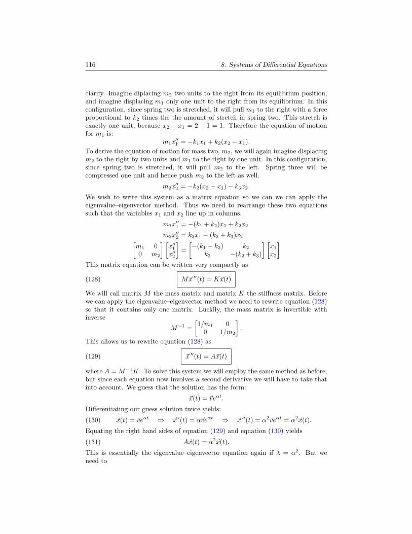
116 8. Systems of Differential Equations
clarify. Imagine diplacing m2 two units to the right from its equilibrium position,and imagine displacing m1 only one unit to the right from its equilibrium. In thisconfiguration, since spring two is stretched, it will pull m1 to the right with a forceproportional to k2 times the the amount of stretch in spring two. This stretch isexactly one unit, because x2 − x1 = 2 − 1 = 1. Therefore the equation of motionfor m1 is:
m1x′′1 = −k1x1 + k2(x2 − x1).
To derive the equation of motion for mass two, m2, we will again imagine displacingm2 to the right by two units and m1 to the right by one unit. In this configuration,since spring two is stretched, it will pull m2 to the left. Spring three will becompressed one unit and hence push m2 to the left as well.
m2x′′2 = −k2(x2 − x1)− k3x2.
We wish to write this system as a matrix equation so we can we can apply theeigenvalue–eigenvector method. Thus we need to rearrange these two equationssuch that the variables x1 and x2 line up in columns.
m1x′′1 = −(k1 + k2)x1 + k2x2
m2x′′2 = k2x1 − (k2 + k3)x2[
m1 00 m2
] [x′′1x′′2
]=
[−(k1 + k2) k2
k2 −(k2 + k3)
] [x1
x2
]This matrix equation can be written very compactly as
(128) M~x ′′(t) = K~x(t)
We will call matrix M the mass matrix and matrix K the stiffness matrix. Beforewe can apply the eigenvalue–eigenvector method we need to rewrite equation (128)so that it contains only one matrix. Luckily, the mass matrix is invertible withinverse
M−1 =
[1/m1 0
0 1/m2
].
This allows us to rewrite equation (128) as
(129) ~x ′′(t) = A~x(t)
where A = M−1K. To solve this system we will employ the same method as before,but since each equation now involves a second derivative we will have to take thatinto account. We guess that the solution has the form:
~x(t) = ~veαt.
Differentiating our guess solution twice yields:
(130) ~x(t) = ~veαt ⇒ ~x ′(t) = α~veαt ⇒ ~x ′′(t) = α2~veαt = α2~x(t).
Equating the right hand sides of equation (129) and equation (130) yields
(131) A~x(t) = α2~x(t).
This is essentially the eigenvalue–eigenvector equation again if λ = α2. But weneed to
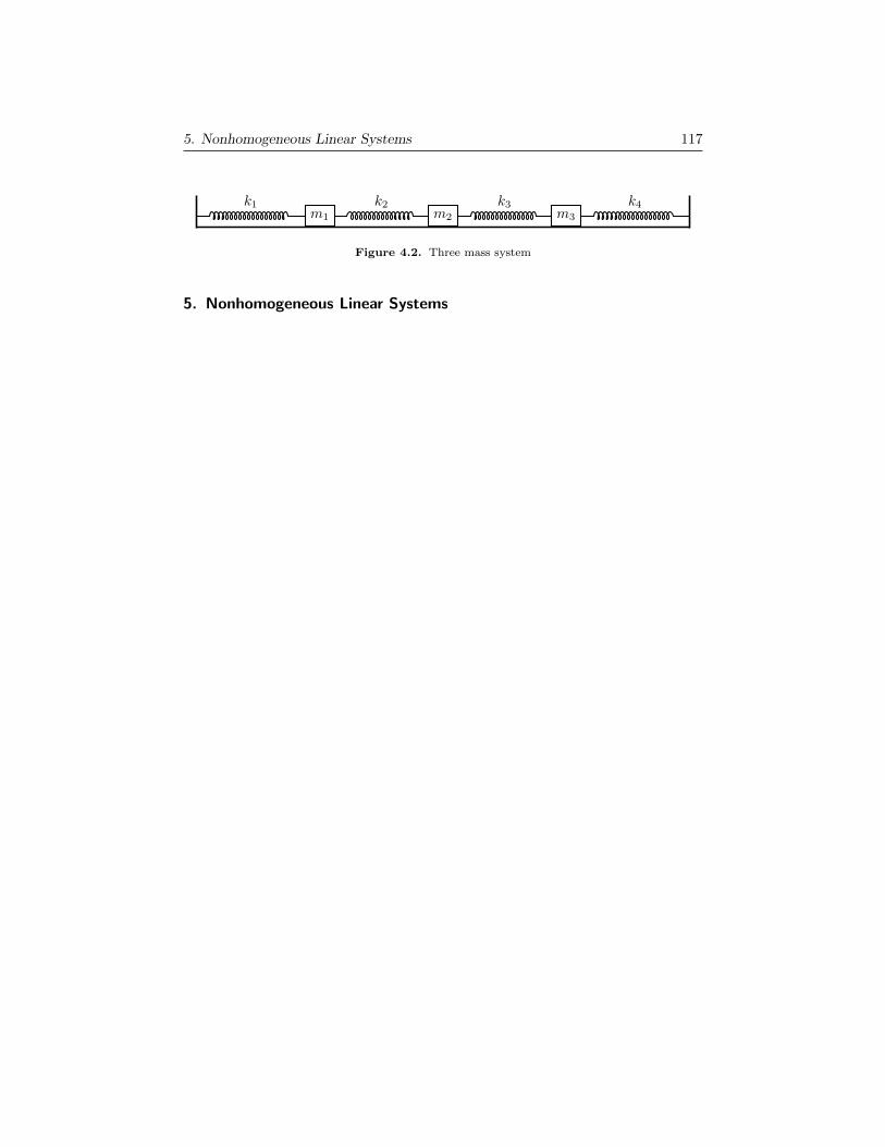
5. Nonhomogeneous Linear Systems 117
m1 m2 m3
k1 k2 k3 k4
Figure 4.2. Three mass system
5. Nonhomogeneous Linear Systems