di erential geometry of curves and...
TRANSCRIPT

Differential Geometryof Curves and Surfaces
Luis Fernandez
Department of Mathematics
University of Bath

Chapter 0
Introduction and preliminaries
The name of this course is Differential Geometry of Curves and Surfaces. Let us analyse each word
to see what it is about.
Geometry is the part of mathematics that studies the ‘shape’ of objects. The name geometry comes
from the greek geo, earth, and metria, measure; in the dawn of mathematics, geometry was the
science of measuring the earth, which has been very important all along history (how can you sell
or buy land if you cannot measure it?). It is, hence, one of the oldest branches of mathematics.
What do we mean by ‘shape’? The Oxford English Dictionary defines shape as ‘External form
or contour; that quality of a material object (or geometrical figure) which depends on constant
relations of position and proportionate distance among all the points composing its outline or its
external surface; a particular variety of this quality.’
So shape is a quality that depends on distances among all points of the object. This implicity says
that when we talk about the shape of an object we do not take into account where it is located
in space: a bottle’s shape is the same whether it is in the rubbish bin or on a table, since the
distances and positions among all points of the bottle do not change.
For our purposes, shape will mean those characteristics of an object that are independent of
position. In other words, if I take a surface, and I rotate it and/or translate it, the surface I obtain
has the same shape as the original one. These movements of in space (rotations and translations)
are called rigid motions.
In this course we will deal with curves living in the plane and in three-dimensional space as well
as with surfaces living in three-dimensional space. A curve in space is essentially the shape that a
wire would take. A surface is the shape that soap film, for example, takes.
It only remains to explain the word ‘differential’. In order to measure the length of curves that live,
say, in a surface, we need to give a meaning to the concept of velocity. Velocity is exactly what we
express with the derivative (or ‘differential’), as you may know from early calculus courses. So it
means that in this course we will study the shape of curves making heavy use, among other things,
of derivatives and concepts that are studied in calculus courses.
The curves and surfaces we will study are expressed with formulas; for example, a circle of radius 2
in the plane can be expressed as the set of points (x, y) ∈ R2 such that x2 + y2 = 4. Alternatively
it can be expressed as the image of the map α : R → R2 given by
α(t) = (2 cos t, 2 sin t).
A sphere of radius 1 can be expressed as the set of points (x, y, z) ∈ R3 such that x2 + y2 + z2 = 1.
3
4 CHAPTER 0. INTRODUCTION AND PRELIMINARIES
Alternatively, it can be seen as the image of the map. σ : R2 → R
3 given by
σ(θ, φ) = (cos φ cos θ, cosφ sin θ, sin φ).
These examples show that there are several ways to describe geometrical objects. We will use both
ways, although most times the second, i.e. expressing the object as the image of a map, will be more
suitable for calculations. This way of expressing geometric objects is called a ‘parametrization’,
which gets this name from the fact that it introduces parameters (t in the example of the circle
and φ and θ in the example of the sphere).
Since our geometric objects will live in the plane (R2) or in the space (R3), let us first review some
facts about the vector space Rn.
0.0.1 Review of geometry and linear algebra
The set Rn is the set of all n-tuples of real numbers. With the usual componentwise addition and
multiplication by scalars it has the structure of a vector space, so its elements are called vectors. We
will often also call them points, depending on whether we want to emphasise a direction (vectors,
denoted like ~v) or a location (points, denoted like p). It should not be forgotten that both ~v and
p are elements of Rn. [Strictly speaking, points are elements of R
n when we think of it as affine
space, which is something like a vector space not necessarily having a 0, i.e. without a reference
point. Rn is an affine space too.]
Length, norms and scalar (dot) product
• The length or norm or module of a vector ~v = (v1, v2, . . . , vn) is defined as
‖~v‖ =√
v21 + v2
2 + · · · + v2n.
• The distance between two points p and q in Rn is the module of their difference, i.e.
d(p, q) = ‖p − q‖.
• The scalar (or dot) product of two vectors ~u,~v ∈ Rn is
~u · ~v = u1v1 + u2v2 + · · · + unvn.
The dot product is often also denoted as 〈~u,~v〉. Note that ‖~v‖2 = ~v · ~v.
• Note that if we think of vectors in Rn as n by 1 matrices (i.e. column vectors), then
~u · ~v = ~u t ~v, where the t denotes ‘transpose’ and the product on the right term is matrix
multiplication.
If A is a matrix and we denote its column vectors as ~a1,~a2, . . . ,~an (so that A could be written
as (~a1,~a2, . . . ,~an)) then we have
At A = (~a1,~a2, . . . ,~an)t(~a1,~a2, . . . ,~an) =
(~a1 · ~a1) (~a1 · ~a2) · · · (~a1 · ~an)(~a2 · ~a1) (~a2 · ~a2) · · · (~a2 · ~an)
......
. . ....
(~an · ~a1) (~an · ~a2) · · · (~an · ~an)
• The scalar product satisfies |~u · ~v| = ‖~u‖‖~v‖ cos θ, where θ is the angle between ~u and ~v.
• The standard basis of Rn will be denoted by {~e1, ~e2, . . . , ~en}. Recall that ~ei is an n-tuple of
all 0’s with a 1 in the ith position. In R3 the notation {~ı,~, ~k} is also common and we may
use it at times.
5
• A basis {~v1, ~v2, . . . , ~vn} is called orthonormal if ~vi · ~vj = δij . (Recall that δij is Kronecker’s
delta, i.e. a function with two integer entries (i and j) that takes the value 0 if i 6= j and 1
if i = j.)
• If {~v1, ~v2, . . . , ~vn} is an orthonormal basis and ~u is any vector, then we can express ~u in terms
of the basis as
~u = (~u · ~v1) ~v1 + (~u · ~v2) ~v2 + · · · + (~u · ~vn) ~vn.
Vector (cross) product
The vector or cross product of two vectors, ~u = (u1, u2, u3) and ~v = (v1, v2, v3) in R3 is defined as
~u × ~v = (u2v3 − u3v2, u3v1 − u1v3, u1v2 − u2v1).
The vector product of two vectors is only defined in R3. It has the following properties.
• ~u × ~v = −~v × ~u
• ~u × ~v = ~0 ⇐⇒ ~u and ~v are linearly dependent (i.e. parallel or one of them is ~0).
• ~u × ~v is perpendicular to both ~u and ~v.
• ‖~u×~v‖ = ‖~u‖‖~v‖ sin θ (θ is the angle between ~u and ~v) and this quantity also gives the area
of the parallelogram spanned by the vectors ~u and ~v.
• (~u × ~v) · ~w is the determinant of the matrix whose columns are the components of ~u, ~v and
~w in this order. The absolute value of this number gives the volume of the parallelepiped
spanned by ~u, ~v and ~w.
• An orthonormal basis {~v1, ~v2, ~v3} of R3 is positively oriented if ~v3 = ~v1 × ~v2, and negatively
oriented if ~v3 = −~v1 ×~v2 (note that these are the only two possibilities since ~v3 and −~v3 are
the only two unit vectors othogonal to both ~v1 and ~v2). Note that the standard basis of R3
is positively oriented.
Linear maps and matrices
A linear map L : Rn → R
m is one that satisfies L(a~u + b~v) = aL(~u) + bL(~v) for ~u,~v ∈ Rn and
a, b ∈ R. In terms of bases of Rn and R
m, linear maps are represented by matrices.
DEFINITION 0.0.1 A matrix A is orthogonal if it is a square matrix that satisfies A At = At A =
I, where the superscript t stands for the transpose and I is the identity matrix.
A linear map L : Rn → R
n is orthogonal if its matrix in terms of the standard bases of Rn and
Rm is orthogonal.
If A is an orthogonal matrix, det(A)2 = det(A) det(At) = det(A At) = det(I) = 1, so det(A) is
either 1 or −1. The set of orthogonal n by n matrices is denoted O(n, R); the set of orthogonal n
by n matrices with determinant 1 is denoted SO(n, R).
If A is an orthogonal matrix,
• (A~u) · (A~v) = (~u)tAtA~v = (~u)t~v = ~u · ~v. This implies that orthogonal maps leave lengths
invariant: ‖A~v‖ = ‖~v‖.
6 CHAPTER 0. INTRODUCTION AND PRELIMINARIES
• (A~u) × (A~v) = det(A) A (~u × ~v). This can be proved as follows: if ~w ∈ R3 is any vector,
~w · (A~u) × (A~v) = [ (AA−1 ~w)] · [(A~u) × (A~v)]
= det[A (At ~w), A~u, A~v]
= det(A) det(At ~w, ~u,~v)
= det(A) ((At ~w) · (~u × ~v))
= det(A) ((At ~w)t(~u × ~v))
= det(A) (~wt A (~u × ~v))
= det(A) (~w · (A(~u × ~v))
Reordering we have
~w · [((A~u) × (A~v)) − det(A) (A(~u × ~v))] = 0
for any vector ~w. Therefore,
((A~u) × (A~v)) − det(A) A(~u × ~v) = 0,
as desired.
• If { ~u1, ~u2, ~u3} and {~v1, ~v2, ~v3} are orthonormal bases of R3 then there is a unique orthogonal
matrix A with A ~u1 = ~v1, A ~u2 = ~v2, A ~u3 = ~v3. [In fact this matrix is, writing all vectors as
columns in terms of the standard basis, (~v1, ~v2, ~v3) ( ~u1, ~u2, ~u3)t.] This matrix has determinant
1 if both bases are have the same orientation (either positive or negative) and determinant
−1 if they have different orientations. (This is in general for Rn although we only stated it
for R3).
DEFINITION 0.0.2
• A translation in Rn is a map T : R
n → Rn of the form T (p) = p + ~v for some vector ~v in
Rn. It is just moving all points of R
n by the vector ~v.
• A rigid motion in Rn is the composition of a translation and an orthogonal transformation
of determinant 1.
• An isometry of Rn is a map from R
n to Rn that preserves distance between points. This is,
G is an isometry if and only if ‖G(p) − G(q)‖ = ‖p − q‖.
It is an important theorem that we will not prove that the only isometries of Rn are compositions
of translations and orthogonal transformations.
0.0.2 Calculus
The most general definition of differentiability is the following.
DEFINITION 0.0.3 A map f : U ⊂ Rn → R
m is differentiable at a point p ∈ U if there exists a
linear function Dfp : Rn → R
m such that
lim~h→~0
f(p + ~h) − f(p) − Dfp(~h)
‖~h‖= 0
The linear map Dfp is called the derivative of f at p. The matrix associated to Dfp when we
write it in terms of the standard basis is denoted Jfp (the Jacobian matrix).
7
Recall that the partial derivative of a function at the point p with respect to its kth entry, denoted
Dkfp, is the derivative of the function with respect to that entry when we consider all the other
entries as constants. If the kth entry is called xk, this is traditionally denoted as
∂f
∂xk
(p) or∂f
∂xk p
.
Although you may not be used to it, the notation Dkfp is generally better than the traditional
one because it does not assume any predefined name of the variables. We had to assume that the
kth variable was called xk in order to use the traditional notation. This often leads to errors when
using the chain rule.
When f is a function of a single variable, we normally use the notation f ′(p) for the derivative of
f at p.
The entry at position (ij) of the matrix Jfp is given by (using traditional notation)
(Jfp)ij =∂fi
∂xjp
.
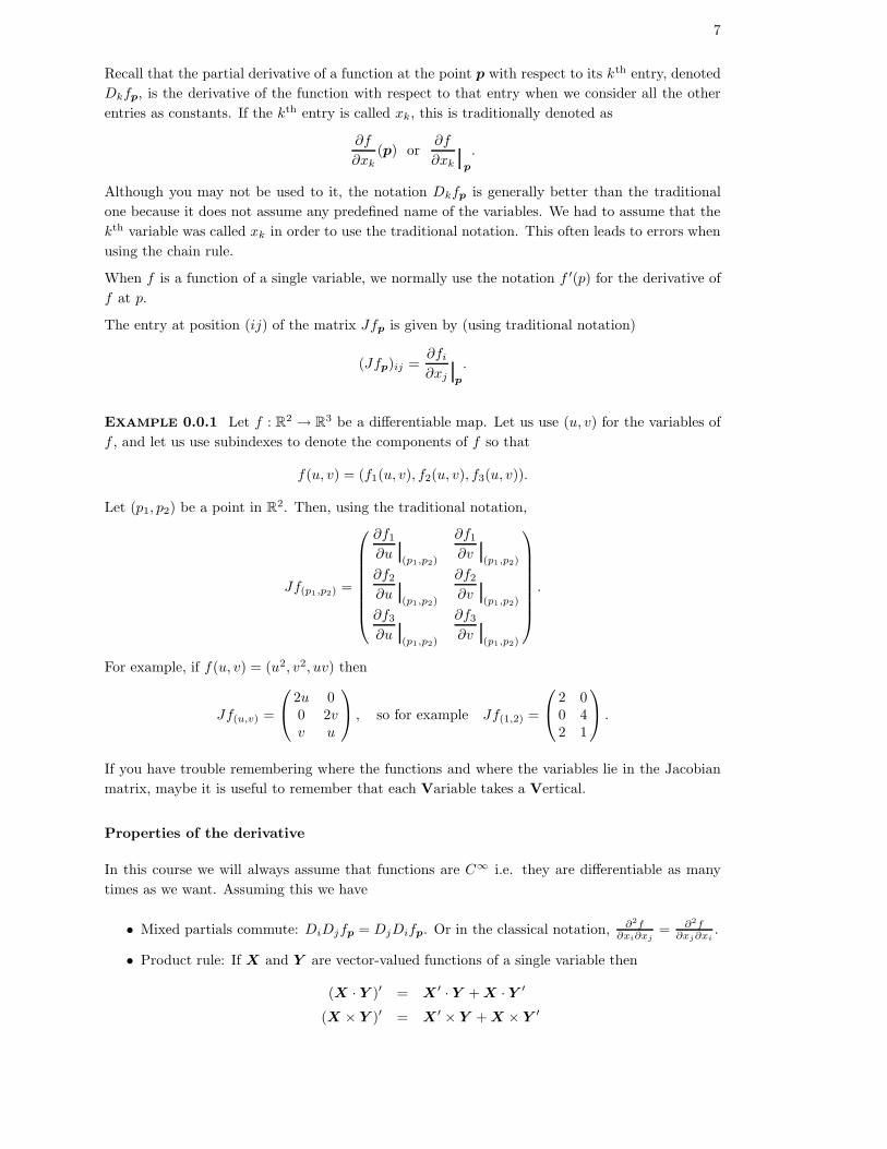
EXAMPLE 0.0.1 Let f : R2 → R
3 be a differentiable map. Let us use (u, v) for the variables of
f , and let us use subindexes to denote the components of f so that
f(u, v) = (f1(u, v), f2(u, v), f3(u, v)).
Let (p1, p2) be a point in R2. Then, using the traditional notation,
Jf(p1,p2) =
∂f1
∂u(p1,p2)
∂f1
∂v(p1,p2)
∂f2
∂u(p1,p2)
∂f2
∂v(p1,p2)
∂f3
∂u(p1,p2)
∂f3
∂v(p1,p2)
.
For example, if f(u, v) = (u2, v2, uv) then
Jf(u,v) =
2u 00 2vv u
, so for example Jf(1,2) =
2 00 42 1
.
If you have trouble remembering where the functions and where the variables lie in the Jacobian
matrix, maybe it is useful to remember that each Variable takes a Vertical.
Properties of the derivative
In this course we will always assume that functions are C∞ i.e. they are differentiable as many
times as we want. Assuming this we have
• Mixed partials commute: DiDjfp = DjDifp. Or in the classical notation, ∂2f∂xi∂xj
= ∂2f∂xj∂xi
.
• Product rule: If X and Y are vector-valued functions of a single variable then
(X · Y )′ = X ′ · Y + X · Y ′
(X × Y )′ = X ′ × Y + X × Y ′

8 CHAPTER 0. INTRODUCTION AND PRELIMINARIES
• Chain rule: In terms of linear maps, D(f ◦ g)p = Dfg(p) ◦ Dgp. In terms of matrices,
J(f ◦g)p = Jfg(p) Jgp (product of matrices in the last term). In terms of partial derivatives,
in classical notation, using y’s to denote the entries of f and x’s to denote the entries of g,
we have∂(fi ◦ g)
∂xj p
=∑
k
∂fi
∂yk g(p)
∂gk
∂xj p
.
An interpretation of the linear map Dfp is as follows. If we are travelling along a curve α(t) with
velocity vector ~v at time t0 (so α′(t0) = ~v) then, if we suddenly get ‘teletransported’ via the map
f we will be moving with velocity vector equal to
(f ◦ α)′(t0) = Dfα(t0)(α′(t0)) = Dfα(t0)(~v).
So Dfp tells us how velocities in p transform when we apply the function f .
For the purposes of this course we will need the following.
DEFINITION 0.0.4 A map f : Rn → R
m is called regular at a point p if Dfp has maximal rank
or, in terms of matrices, the matrix Jfp has maximal rank. Recall that this means that, if m ≥ n,
the n columns of Jfp are linearly independent, and if m < n, the m rows of Jfp are linearly
independent.
A map f is said to be a regular map if it is regular at all the points of its domain.
We will be primarily interested in maps f : R2 → R
3. In this case, f will be regular at a point p
if and only if the vectors D1fp and D2fp in R3 are linearly independent. Since two vectors in R
3
are linearly independent if and only if their cross product is not zero, this can also be expressed as
D1fp × D2fp 6= ~0
or, in the traditional notation, using u and v as the variables of f ,
∂f
∂up
× ∂f
∂vp
6= ~0.
0.0.3 Topology
Topology is the branch of mathematics concerned with continuous functions and everything that
does not change under continuous deformations. We only need a few definitions.
DEFINITION 0.0.5
• An open ball centered at p with radius r in Rn is a set of the form
Br(p) = {x ∈ Rn : ‖x − p‖ < r},
i.e. it consists of all points at a distance less than r from p.
• A subset U of Rn is called open if about every point of U there is an open ball containing the
point that is completely contained in U .
• Given a subset M of Rn, a subset V of M is called open if it has the form V = M ∩U , where
U is an open subset of Rn.

9
This definition is quite technical, as you can see, and will be studied in more detail in further
courses. You just need to think of an open set as one in which, given a point, we can get to
this point from nearby points in all possible directions without leaving the set. For example, the
interval (0, 1] (i.e. 1 is included), is not open: we cannot reach 1 from the right without leaving
the set.
Now we define continuity.
DEFINITION 0.0.6 Let M and N be subsets of Rm and R
n, respectively. A map f : M → N is
• Continuous at p if
limx→p
f(x) = f(p).
(Roughly this means that if we get close to p while staying in M , then the value of f will be
close to f(p) regardless of the way in which we get close to p)
If the map f is continuous at every point, then it is just called continuous.
• A homeomorphism if
– It is continuous.
– It is bijective (i.e. one-to-one and onto).
– Its inverse is also continuous.
Two sets are called homeomorphic if there exists a homeomorphism between them.
Roughly speaking, two sets are homeomorphic if we can deform one into the other without breaking
or glueing anything. For example, a circle and an ellipse are homeomorphic.
NOTE: These definitions are rather technical and difficult. We will only need a general idea of
these concepts for the rest of the course. They are here for the sake of completeness—without
them we would not be able to give a rigorous definition of surfaces, for example. But we do not
want to spend much time on them, as you will learn all about topology in more advanced courses.

10 CHAPTER 0. INTRODUCTION AND PRELIMINARIES
Chapter 1
Curves
1.1 Regular curves and parametrised curves
DEFINITION 1.1.1 A parametrised curve is a smooth map α : (a, b) → Rn, where −∞ ≤ a <
b ≤ ∞ (i.e. a can be −∞ and/or b can be ∞).
A parametrised curve α is called regular if in addition the derivative of α is never 0.
Recall that ‘smooth’ means ‘infinitely differentiable’, i.e. we can take as many derivatives of α
as we desire. We could have defined parametrised curves without this smoothness condition, but
then we would have extremely messy objects about which not many general facts can be said.
So in general all the parametrised curves in this course will be smooth (i.e. infinitely
differentiable) maps.
The (regularity) condition α′ 6= 0 in the definition of parametrised regular curve is added to avoid
cusps and corners.
Note that the above is not the way we think of curves in life. We never think of curves as maps,
rather as a set of points in space. This is why we put the modifier ‘parametrised’ in the previous
definition. Following this idea, a curve would be more likely defined as follows:
DEFINITION 1.1.2 A regular curve is a subset C of Rn such that, for every p ∈ S there is an
open set U ⊂ Rn, with p ∈ U , and there is a smooth, one-to-one and onto map α : (a, b) → C ∩ U
whose derivative is never 0.
Let us unrevel the definition of a regular curve. It is a subset of space, which is intuitively the
way we think of curves. The rest of the definition means that, locally (i.e. about any point of the
curve), the curve is a parametrised regular curve as defined before.
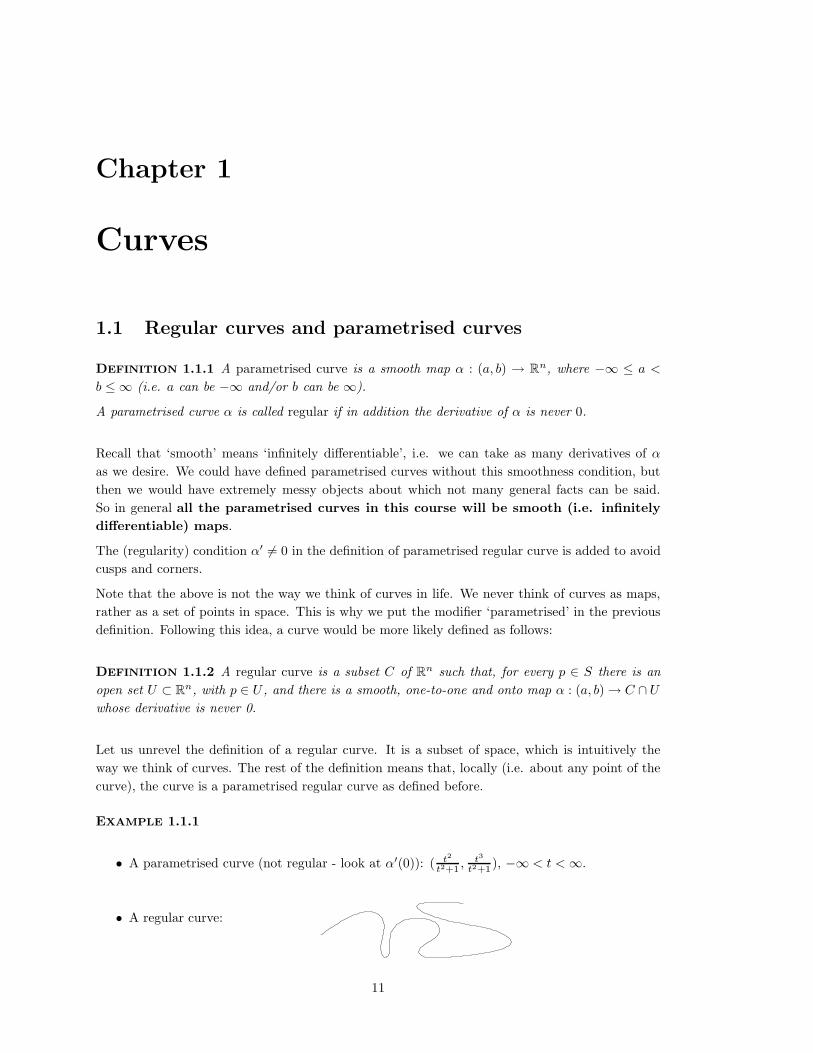
EXAMPLE 1.1.1
• A parametrised curve (not regular - look at α′(0)): ( t2
t2+1 , t3
t2+1 ), −∞ < t < ∞.
• A regular curve:
11

12 CHAPTER 1. CURVES
Note that regular curves cannot have self-intersections: if they did, about the point of intersection
the curve would look like an X, and there cannot be a one-to-one and onto smooth map from an
interval to an X. Parametrised curves, instead, can have self intersections.
EXAMPLE 1.1.2
• A regular parametrised curve with a self intersection: (sin t, sin 2t), −∞ < t < ∞.
The difference between parametrized curves and regular curves is not very important, since every
regular curve can be seen as the image of a parametrised curve, so our study will concentrate in
parametrised curves.
Note that if we have a parametrised curve α and we pre-compose it with a function φ from R to
R, we obtain a different parametrised curve α = α ◦ φ with the same ‘trace’ as the original one.
Then α will be called a reparametrization of α. For example, given the curve
α(t) = (cos t, sin t, t), for −∞ < t < ∞
we can compose it with the function φ(s) = 3s to obtain the parametrised curve
α(s) = (cos 3s, sin 3s, 3s).
The trace of both α and α is the same: a ‘helix’.
In our study of the ‘shape’ of curves we would like to think of curves with
the same trace as equal. If the image of the maps is the same, why should
we think of them as different? Hence all the properties that we will study
will be independent of reparametrization.
DEFINITION 1.1.3 Let α : (a, b) → Rn be a parametrised curve, and let φ : (a′, b′) → (a, b) be a
differentiable bijective function whose derivative is never 0. The parametrised curve α : (a′, b′) →R
n defined by α(t) = α(φ(t)) is called a reparametrisation of α.
1.2 Velocity vector
Given a parametrised curve α : (a, b) → Rn, its derivative α′(t) at some t ∈ (a, b) will be a vector
in Rn that gives the velocity of α at t. We can think of α′(t) as a vector anchored at the point
α(t):
(t)α α ’(t)
The tangent line to α at the point α(t0) is the line
`(s) = α(t0) + sα′(t0).
While a reparametrisation of a curve leaves the trace of the curve invariant, what does it do to the
velocity? Since the velocity is the derivative, we only have to take derivatives to α and apply the
chain rule:
α′(t) = α′(φ(t)) φ′(t).
1.3. ARC LENGTH 13
Thus the velocity vector will be multiplied by φ′(t). In other words, if we are travelling along α(s),
where we think of the parameter s as the time, we will do the same trajectory as if we travel along
α(t) but we will be at different places in different moments, and our speed is likely to be different
at each point of the curve. Note that we used different parameters t and s, related by s = φ(t),
only to emphasise the fact that our time frame is different in each case.
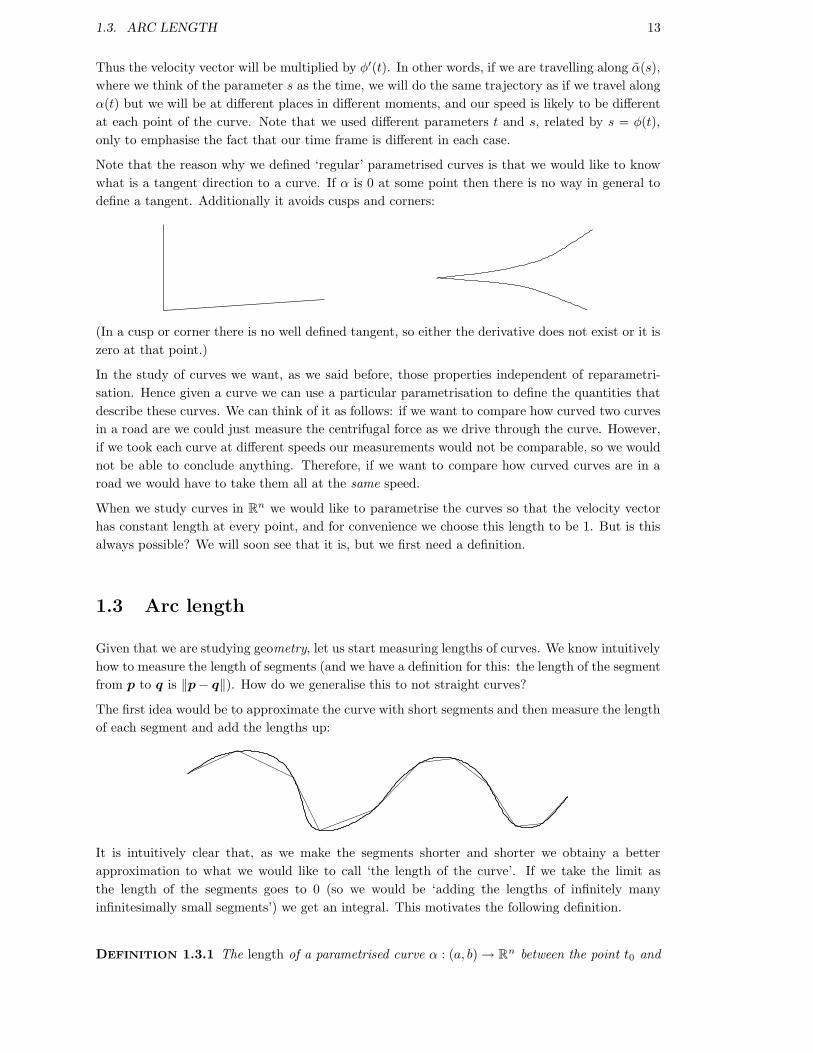
Note that the reason why we defined ‘regular’ parametrised curves is that we would like to know
what is a tangent direction to a curve. If α is 0 at some point then there is no way in general to
define a tangent. Additionally it avoids cusps and corners:
(In a cusp or corner there is no well defined tangent, so either the derivative does not exist or it is
zero at that point.)
In the study of curves we want, as we said before, those properties independent of reparametri-
sation. Hence given a curve we can use a particular parametrisation to define the quantities that
describe these curves. We can think of it as follows: if we want to compare how curved two curves
in a road are we could just measure the centrifugal force as we drive through the curve. However,
if we took each curve at different speeds our measurements would not be comparable, so we would
not be able to conclude anything. Therefore, if we want to compare how curved curves are in a
road we would have to take them all at the same speed.
When we study curves in Rn we would like to parametrise the curves so that the velocity vector
has constant length at every point, and for convenience we choose this length to be 1. But is this
always possible? We will soon see that it is, but we first need a definition.
1.3 Arc length
Given that we are studying geometry, let us start measuring lengths of curves. We know intuitively
how to measure the length of segments (and we have a definition for this: the length of the segment
from p to q is ‖p− q‖). How do we generalise this to not straight curves?
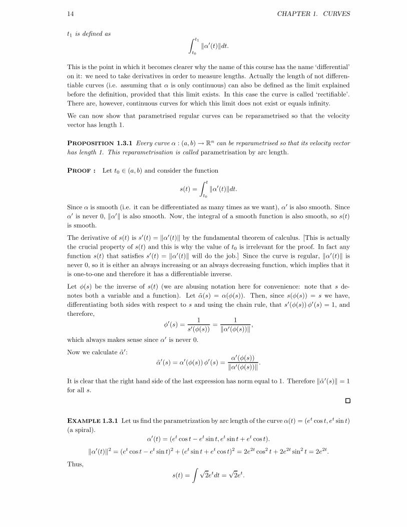
The first idea would be to approximate the curve with short segments and then measure the length
of each segment and add the lengths up:
It is intuitively clear that, as we make the segments shorter and shorter we obtainy a better
approximation to what we would like to call ‘the length of the curve’. If we take the limit as
the length of the segments goes to 0 (so we would be ‘adding the lengths of infinitely many
infinitesimally small segments’) we get an integral. This motivates the following definition.
DEFINITION 1.3.1 The length of a parametrised curve α : (a, b) → Rn between the point t0 and
14 CHAPTER 1. CURVES
t1 is defined as∫ t1
t0
‖α′(t)‖dt.
This is the point in which it becomes clearer why the name of this course has the name ‘differential’
on it: we need to take derivatives in order to measure lengths. Actually the length of not differen-
tiable curves (i.e. assuming that α is only continuous) can also be defined as the limit explained
before the definition, provided that this limit exists. In this case the curve is called ‘rectifiable’.
There are, however, continuous curves for which this limit does not exist or equals infinity.
We can now show that parametrised regular curves can be reparametrised so that the velocity
vector has length 1.
PROPOSITION 1.3.1 Every curve α : (a, b) → Rn can be reparametrised so that its velocity vector
has length 1. This reparametrisation is called parametrisation by arc length.
PROOF : Let t0 ∈ (a, b) and consider the function
s(t) =
∫ t
t0
‖α′(t)‖dt.
Since α is smooth (i.e. it can be differentiated as many times as we want), α′ is also smooth. Since
α′ is never 0, ‖α′‖ is also smooth. Now, the integral of a smooth function is also smooth, so s(t)
is smooth.
The derivative of s(t) is s′(t) = ‖α′(t)‖ by the fundamental theorem of calculus. [This is actually
the crucial property of s(t) and this is why the value of t0 is irrelevant for the proof. In fact any
function s(t) that satisfies s′(t) = ‖α′(t)‖ will do the job.] Since the curve is regular, ‖α′(t)‖ is
never 0, so it is either an always increasing or an always decreasing function, which implies that it
is one-to-one and therefore it has a differentiable inverse.
Let φ(s) be the inverse of s(t) (we are abusing notation here for convenience: note that s de-
notes both a variable and a function). Let α(s) = α(φ(s)). Then, since s(φ(s)) = s we have,
differentiating both sides with respect to s and using the chain rule, that s′(φ(s)) φ′(s) = 1, and
therefore,
φ′(s) =1
s′(φ(s))=
1
‖α′(φ(s))‖ ,
which always makes sense since α′ is never 0.
Now we calculate α′:
α′(s) = α′(φ(s)) φ′(s) =α′(φ(s))
‖α′(φ(s))‖ .
It is clear that the right hand side of the last expression has norm equal to 1. Therefore ‖α′(s)‖ = 1
for all s.
EXAMPLE 1.3.1 Let us find the parametrization by arc length of the curve α(t) = (et cos t, et sin t)
(a spiral).
α′(t) = (et cos t − et sin t, et sin t + et cos t).
‖α′(t)‖2 = (et cos t − et sin t)2 + (et sin t + et cos t)2 = 2e2t cos2 t + 2e2t sin2 t = 2e2t.
Thus,
s(t) =
∫ √2etdt =
√2et.
1.4. CURVATURE 15
[Note that here we wrote an improper integral to define s(t). As we said before we only need that
s(t) be an antiderivative of ‖α′(t)‖; for example, we could have also chosen s(t) =√
2et +C, where
C is some constant.] The inverse of s(t) is φ(s) = log(s/√
2), so a reparametrization by arc length
of α is
α =
(
s√2
cos(log(s/√
2)),s√2
sin(log(s/√
2))
)
.
Parametrisations by arc length are not unique, as we saw above. But they only depend on the
‘origin of time’ and the ‘direction of time’, as follows:
LEMMA 1.3.1 If α and β are two reparametrisations by arc length of the same parametrised curve
γ, then either α(s) = β(s + c) or α(s) = β(−s + c), where the letter c stands for some constant.
In the first case we say that the two parametrizations have the same orientation and in the second
we say that they have opposite orientation (the curve is traced in opposite directions).
PROOF : Since α and β are reparametrisations of γ, we must have that α is also a reparametri-
sation of β, this is, α(s) = β(φ(s)) for some smooth bijective function φ. Taking derivatives in
both sides and using the chain rule we obtain
α′(s) = β′(φ(s))φ′(s),
and taking norms we find
1 = ‖α′(s)‖ = ‖β′(φ(s))‖ |φ′(s)| = |φ′(s)|.
Hence either φ′(s) = 1 for all s, which implies φ(s) = s + c for some constant c, and therefore
α(s) = β(s + c) or φ′(s) = −1 for all s, which implies φ(s) = −s + c for some constant c, and
therefore α(s) = β(−s + c). Note that these are the only cases: φ′(s) cannot be 1 for some values
of s and −1 for others since it is a continuous function.
Great! So now we can start measuring things in curves without worrying about whether what we
define is dependent on speed or not: we just take everything to have speed 1 (in these notes, speed
will mean the length of the velocity vector, as it is usually understood).
1.4 Curvature
Our next goal is to make mathematical sense to the question ‘How curved is a curve?’ As we
discussed before, when we are riding in a car we would say that, at same speed, the more curved is
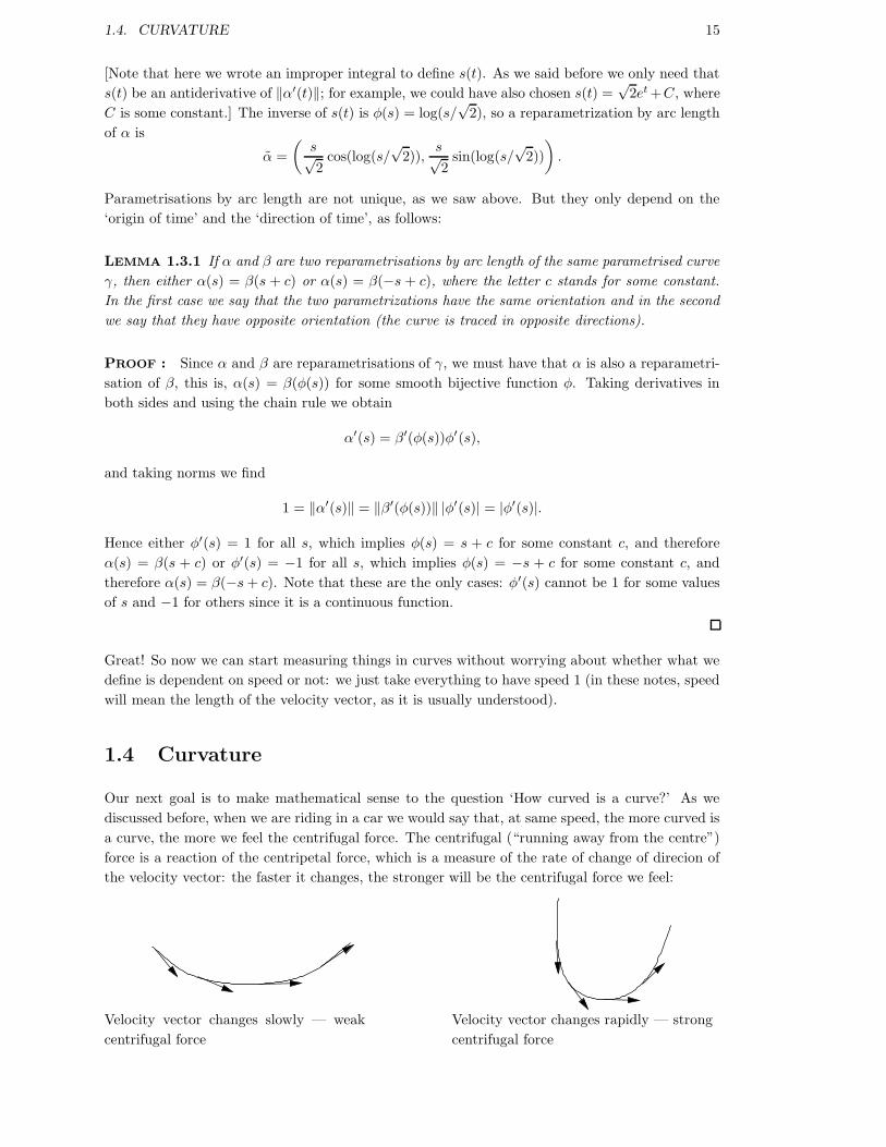
a curve, the more we feel the centrifugal force. The centrifugal (“running away from the centre”)
force is a reaction of the centripetal force, which is a measure of the rate of change of direcion of
the velocity vector: the faster it changes, the stronger will be the centrifugal force we feel:
Velocity vector changes slowly — weak
centrifugal force
Velocity vector changes rapidly — strong
centrifugal force

16 CHAPTER 1. CURVES
DEFINITION 1.4.1 Let α : (a, b) → Rn be a parametrised curve, parametrised by arc length (i.e.
‖α′(s)‖ = 1 for all s). The curvature of α at the point α(s) is the function
κ(s) = ‖α′′(s)‖.
It is traditionally denoted by the greek letter κ (kappa).
The curvature of a parametrised curve in general is defined as the curvature of any reparametrisa-
tion by arc length of that curve.
Of course this definition only makes sense if the number ‖α′′(s)‖ is independent of the arc length
parametrization of α. But it is easy to see that it is the case: if α and β are reparametrizations
by arc length of the same curve, then by Lemma 1.3.1 we have that α(s) = β(±s + c), so α′(s) =
±β′(±s + c) and α′′(s) = β′′(±s + c). Therefore, ‖α′′(s)‖ = ‖β′′(±s + c)‖ and κ will be equal at
each point of the curve independently of whether it is defined using α or β.
EXAMPLE 1.4.1 Let us find the curvature of the curve α(t) = (et cos t, et sin t) of example 3.1.
The parametrization by arc length of α is α = (√
s cos(log√
s),√
s sin(log√
s)). Hence
κ(s) = ‖α′′(s)‖ =
∥
∥
∥
∥
∥
(
−cos(log(s/√
2)) + sin(log(s/√
2))√2 s
,cos(log(s/
√2)) − sin(log(s/
√2))√
2 s
)∥
∥
∥
∥
∥
=1
s
EXAMPLE 1.4.2 Let us find the curvature of a regular curve in R2 lying in a circumference of
radius R centred at a point p.
Let α be the curve and assume that it is parametrised by arc length. Since it lies in the circum-
ference of radius R centred at a point p, we have
‖α(s) − p‖ = R.
We write the last equation as (α(s) − p) · (α(s) − p) = R2 and we take derivatives in both sides
(remember: if you do not know what to do, take derivatives!). We obtain
2α′(s) · (α(s) − p) = 0,
so α′(s) and (α(s) − p) are perpendicular. Differentiating again,
2α′′(s) · (α(s) − p) + 2α′(s) · α′(s) = 0 so α′′(s) · (α(s) − p) = −α′(s) · α′(s).
On the other hand, α is parametrised by arc length so
‖α′(s)‖2 = α′(s) · α′(s) = 1.
Differentiating the last equation we obtain
2α′(s) · α′′(s) = 0,
and therefore α′′(s) must also be perpendicular to α′(s). Since we are in R2, two vectors per-
pendicular to a given one must be parallel, so (α(s) − p) and α′′(s) must be parallel. Thus we
have
|α′′(s) · (α(s) − p)| = ‖α′′(s)‖ ‖(α(s) − p)‖ = ‖α′(s) · α′(s)‖ = | − 1| = 1.
Since ‖(α(s) − p)‖ = R, we finally obtain
k(s) = ‖α′′(s)‖ =1
R.
1.5. FRENET FRAMES, CURVATURE AND TORSION 17
1.5 Frenet frames, curvature and torsion
If we are riding in a roller coaster all the forces we feel are taken from the point of view of our
reference system, which is riding with us in the roller coaster. So it makes sense to describe relevant
quantities in a curve with a reference frame that is moving with the curve.
Let α be a parametrised regular curve. We define T as the unit tangent vector to α pointing
towards the direction of movement of α. Hence, if α is parametrised by arc length,
T (s) = α′(s).
Although T is a function of the parameter s, we normally think of it as a function on the points
α(s) of the curve. In fact. . .
IMPORTANT NOTE ABOUT ‘ADDRESSES’: all the quantities or vectors we define over the
curves (or over the surfaces in the future) will be considered as defined over the curve itself (i.e.
a function on the points that form the curve). However, each of this points can be addressed, via
a one-to-one parametrization, by a value of the parameter. So although we could use the rather
cumbersome notation T (α(s)), we write the equivalent shorter notation T (s).
When α is not parametrised by arc length, we define T (t) = α′(t)/‖α′(t)‖.Now note the following: if α is parametrised by arc length, then
α′(s) · α′(s) = ‖α′(s)‖2 = 1.
Taking derivatives in both sides we obtain
2α′(s) · α′′(s) = 0.
This implies that either α′′(s) = 0 or is perpendicular to α′(s).
In order to define our moving frame of reference we need three vectors. We already have T . A
good choice for another vector would be the unit vector pointing in the direction of α′′(s). However
we can only do this if α′′(s) 6= 0. So let us restrict our study to curves that satisfy this condition.
DEFINITION 1.5.1 A parametrised regular curve α : (a, b) → Rn, parametrised by arc length, is
called biregular if α′′(s) 6= 0 for all s ∈ (a, b).
A parametrised regular curve α : (a, b) → Rn, NOT necessarily parametrised by arc length, is
called biregular if it has a reparametrization by arc length that is biregular (and hence all its
reparametrizations by arc length will also be biregular—see the remark before example 4.1).
LEMMA 1.5.1 A curve α : (a, b) → Rn is biregular if and only if α′(t) and α′′(t) are linearly
independent for all t.
PROOF : Let α(s) = α(φ(s)) be a reparametrization by arc length of α. Then
α′(s) = α′(φ(s)) φ′(s),
and
α′′(s) = α′′(φ(s)) (φ′(s))2 + α′(φ(s)) φ′′(s).
If α is biregular then α′(s) · α′′(s) = 0 and α′′(s) 6= 0, so α′(s) and α′′(s) must be linearly
independent. But looking at the expressions above this implies that α′(φ(s)) and α′′(φ(s)) must
also be linearly independent; otherwise α′′(φ(s)) would be a multiple of α′(φ(s)) so both α′′(s)
and α′(s) would be multiples of α′(φ(s)), contradicting their linear independence.
Conversely, if α′(t) and α′′(t) are linearly independent then α′′(s) cannot be 0 since it is a linear
combination of α′(t) and α′′(t) with nonzero coefficients (since φ′(s) is never 0).

18 CHAPTER 1. CURVES
Given a parametrised biregular curve, parametrised by arc length, we define
N(s) =α′′(s)
‖α′′(s)‖ .
Note that N has length 1 and is perpendicular to T . Also, by definition of κ, T and N , we have
the formula
T ′ = κN .
Up to this point everything we have done is for curves in Rn, without specifying the values of n.
From now on we have to make a distinction. First, in this course we will only study curves in R2
and R3. The same ideas work, however, for any value of n.
1.5.1 Curves in R2
We have defined the perpendicular vectors T and N that move with the curve. Therefore we
already have a frame of reference for R2, given, for each value of the parameter s, by {T (s), N(s)}.
We already know that T ′(s) = κ(s)N(s). What is the derivative of N?
Since N has length 1, using the same calculation we did for α′, we have that N ′ must be perpen-
dicular to N , and therefore it must be a multiple of T . Now we use the following ‘trick’, which is
important in many calculations about curves:
0 = (T · N)′ = T ′ · N + T · N ′.
Since T ′ = κN , we have
T · N ′ = −κ (N · N) = −κ,
and therefore
N ′ = −κT .
This gives the Frenet-Serret formulas for curves in R2:
{
T ′ = κN
N ′ = −κT
If we think of the vectors T and N as column vectors in R2, written in some basis, then these
equations can be written in matrix form as
(T , N)′ = (T , N)
(
0 −κκ 0
)
.
It turns out that κ characterises completely the shape of biregular curves in R2. In other words,
if we know κ, then we can describe the curve completely (although we will not know where it is
located in the plane). But this is a consequence of a similar theorem in R3, so let us first study
curves in R3.
1.5.2 Curves in R3
A reference frame in space consists of three vectors. Given a biregular parametrised curve α we
already defined the perpendicular unit vectors T and N . A sensible choice for a third vector, so
that it is unit and perpendicular to both T and N is
B = T × N ,
1.5. FRENET FRAMES, CURVATURE AND TORSION 19
where × is the cross product in R3.
The frame {T , N , B} is called the Frenet frame of α. Note that it is positively oriented, i.e. in
the same way as the standard coordinate vectors in R3.
Let us calculate the derivative of B. This calculation is a good example of how to calculate
derivatives of vector fields over a curve. First, let us express B ′ in the frame {T , N , B}:
B′ = (B′ · T ) T + (B′ · N) N + (B′ · B) B.
As before, since B · B = 1, differentiating both sides we find that B ′ · B = 0.
On the other hand, B = T × N , so differentiating both sides we obtain
B′ = T ′ × N + T × N ′ = κN × N + T × N ′ = T × N ′.
Hence B′ is perpendicular to T , and therefore B′ ·T = 0. Therefore we have that B′ is a multiple
of N , so we write
B′ = −τN ,
where τ = −B′ ·N . There is no clear reason for the minus sign, it is just custom. The function τ
is called the torsion.
We already know T ′ and B′. Let us now find N ′, using the same strategy as before. We write
N ′ = (N ′ · T ) T + (N ′ · N) N + (N ′ · B) B.
As before, N ′ · N = 0 since N has length 1. To find T · N ′ we do
0 = (T · N)′ = T ′ · N + T · N ′ = κN · N + T · N ′ = κ + T · N ′.
Therefore we have T · N ′ = −κ.
Doing the same with B instead of T we find
0 = (B · N)′ = B′ · N + B · N ′ = −τN · N + B · N ′ = −τ + B · N ′.
Therefore we have B · N ′ = τ .
We can summarise these results in the following
THEOREM 1.5.1 (Frenet-Serret equations) Let α be a biregular curve in R3, parametrised by arc
length. Let T = α′, κ = ‖T ′‖, N = T ′/κ, B = T × N and τ = B · N ′. Then we have
T ′ = κN
N ′ = −κT + τB
B′ = −τN
If we think of the vectors T , N and B as column vectors in R3 written in some basis then these
equations can be written in matrix form as
(T , N , B)′ = (T , N , B)
0 −κ 0κ 0 −τ0 τ 0
.
REMARK 1.5.1 The Frenet-Serret equations for curves in the plane are a particular case of those
in space, as follows.
Given a plane curve in R2 we can embed this R
2 in R3 as the xy-plane to obtain a curve in space.
The vectors T and N will then lie in the xy-plane. Since B is perpendicular to both T and N ,
20 CHAPTER 1. CURVES
it must be perpendicular to the xy-plane. Since it is also unitary, it has to be either (0, 0, 1) or
(0, 0,−1). But then we have
B′ = (0, 0,±1)′ = 0,
which implies that the torsion, τ , is 0, so the Frenet-Serret equations read
T ′ = κN
N ′ = −κT
B′ = 0,
which say exactly the same about T and N as the Frenet-Serret equations in R2.
This will imply that all local properties of curves in R2 can be deduced as a particular case of
curves in R2.
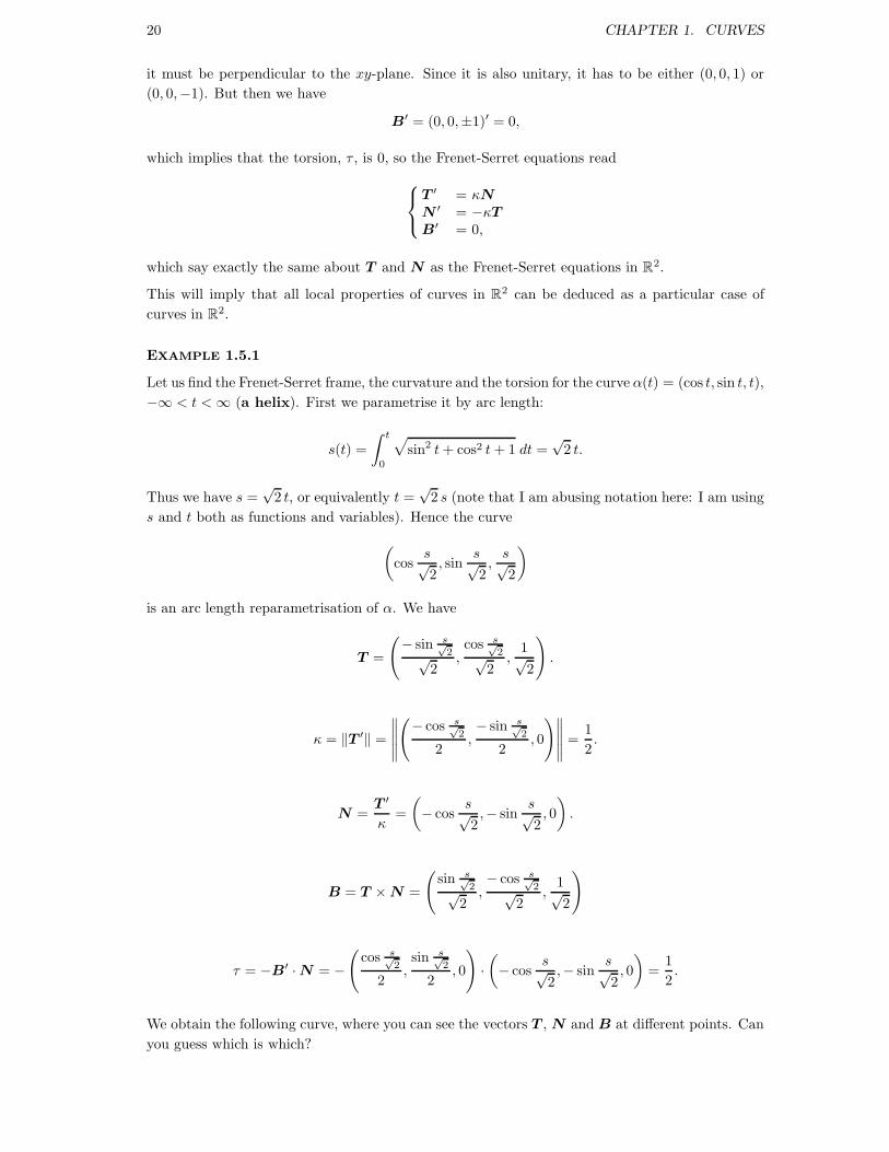
EXAMPLE 1.5.1
Let us find the Frenet-Serret frame, the curvature and the torsion for the curve α(t) = (cos t, sin t, t),
−∞ < t < ∞ (a helix). First we parametrise it by arc length:
s(t) =
∫ t
0
√
sin2 t + cos2 t + 1 dt =√
2 t.
Thus we have s =√
2 t, or equivalently t =√
2 s (note that I am abusing notation here: I am using
s and t both as functions and variables). Hence the curve
(
coss√2, sin
s√2,
s√2
)
is an arc length reparametrisation of α. We have
T =
(
− sin s√2√
2,cos s√
2√2
,1√2
)
.
κ = ‖T ′‖ =
∥
∥
∥
∥
∥
(
− cos s√2
2,− sin s√
2
2, 0
)∥
∥
∥
∥
∥
=1
2.
N =T ′
κ=
(
− coss√2,− sin
s√2, 0
)
.
B = T × N =
(
sin s√2√
2,− cos s√
2√2
,1√2
)
τ = −B′ · N = −(
cos s√2
2,sin s√
2
2, 0
)
·(
− coss√2,− sin
s√2, 0
)
=1
2.
We obtain the following curve, where you can see the vectors T , N and B at different points. Can
you guess which is which?

1.5. FRENET FRAMES, CURVATURE AND TORSION 21
1.5.3 Formulas for curves not parametrised by arc length
To find the curvature and torsion in the last example we had to first reparametrise the curve by arc
length. This is annoying and sometimes extremely hard, since we have to integrate. The following
are general formulas that are valid for any parametrisation of the curve.
PROPOSITION 1.5.1 Let α : (a, b) → R3 be a biregular parametrised curve. Let Sp(t) = ‖α′(t)‖
(the speed of α). Then
α′ = Sp T α′′ = Sp′ T + Sp2 κ N
α′′′ = (Sp′′ − κ2 Sp3) T + (3 Sp Sp′ κ + Sp2 κ′) N + Sp3 κ τ B,
where all the derivatives are taken with respect the parameter t.
PROOF : Let α(s) be a reparametrization by arc length of α so that α(t) = α(s(t)), where s(t)
is the arc length function of α. We have s′(t) = ‖α′(t)‖ = Sp(t). We take derivatives carefully
applying the chain rule and patiently simplify:
α′(t) = α′(s(t)) s′(t) = Sp(t) T (s(t)).
α′′(t) = [Sp(t)]2 T ′(s(t)) + Sp′(t) T (s(t)) = Sp′(t) T (s(t)) + [Sp(t)]2 κ(t) N(s(t)).
α′′′(t) = Sp′′(t) T (s(t)) + Sp(t) Sp′(t) T ′(s(t)) + 2Sp(t) Sp′(t) κ(t) N(s(t))
+[Sp(t)]2 κ′(t) N(s(t)) + [Sp(t)]3 κ(t) N ′(s(t))
= Sp′′(t) T (s(t)) + 3 Sp(t) Sp′(t) κ(t) N(s(t)) + [Sp(t)]2 κ′(t) N(s(t))
+[Sp(t)]3 κ(t)(
−κ(t) T (s(t)) + τ(t) B(s(t)))
=(
Sp′′(t) − [Sp(t)]3 [κ(t)]2)
T (s(t)) +(
3 Sp(t) Sp′(t) κ(t) + [Sp(t)]2 κ′(t))
N(s(t))
+[Sp(t)]3 κ(t) τ(t) B(s(t))
PROPOSITION 1.5.2 Let α : (a, b) → R3 be a biregular parametrised curve. Then
T (t) =α′(t)
Sp(t)B(t) =
α′(t) × α′′(t)
‖α′(t) × α′′(t)‖ N = B × T κ =‖α′ × α′′‖‖α′‖3
τ =(α′ × α′′) · α′′′
‖α′ × α′′‖2.
22 CHAPTER 1. CURVES
PROOF : The first equation is immediate from Propositon 1.5.1. Also from Propositon 1.5.1 we
obtain
α′ × α′′ = Sp3 κ2 T × N = Sp3 κ2 B.
Since Sp3 κ2 > 0, ‖α′ × α′′‖ = Sp3 κ2 and we obtain the desired expression.
N = B × T since by definition B = T × N .
For the expression for κ, using Propositon 1.5.1 we have
α′ × α′′ = Sp3 κ T × N .
Taking norms we obtain
κ =‖α′ × α′′‖
Sp3=
‖α′ × α′′‖‖α′‖3
.
The expression for τ comes from calculating (α′ × α′′) · α′′′ and using Proposition 1.5.1:
(α′ × α′′) · α′′′ = Sp3 κ (T × N) · α′′′
= Sp6 κ2 τ (B · B) (the other terms dissapear)
= ‖α′‖6
(‖α′ × α′′‖‖α′‖3
)2
τ,
from where we get the desired expression.
1.5.4 What are curvature and torsion good for?
We still have not justified our interest in the curvature and torsion. It turns out that these two
functions tell us everything about the shape of the curve. Before proving this fact, we will prove a
few results that are enlightening for understanding what curvature and torsion mean geometrically.
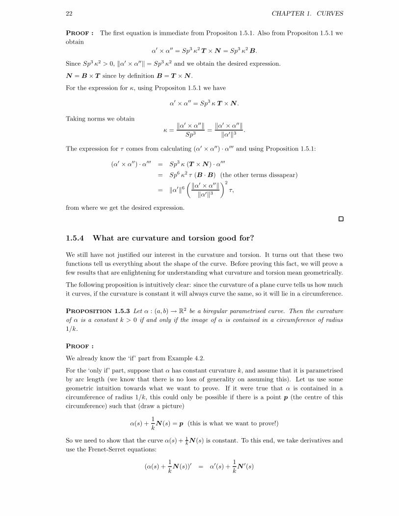
The following proposition is intuitively clear: since the curvature of a plane curve tells us how much
it curves, if the curvature is constant it will always curve the same, so it will lie in a circumference.
PROPOSITION 1.5.3 Let α : (a, b) → R2 be a biregular parametrised curve. Then the curvature
of α is a constant k > 0 if and only if the image of α is contained in a circumference of radius
1/k.
PROOF :
We already know the ‘if’ part from Example 4.2.
For the ‘only if’ part, suppose that α has constant curvature k, and assume that it is parametrised
by arc length (we know that there is no loss of generality on assuming this). Let us use some
geometric intuition towards what we want to prove. If it were true that α is contained in a
circumference of radius 1/k, this could only be possible if there is a point p (the centre of this
circumference) such that (draw a picture)
α(s) +1
kN(s) = p (this is what we want to prove!)
So we need to show that the curve α(s) + 1kN(s) is constant. To this end, we take derivatives and
use the Frenet-Serret equations:
(α(s) +1
kN(s))′ = α′(s) +
1
kN ′(s)
1.5. FRENET FRAMES, CURVATURE AND TORSION 23
= T (s) +1
k(−k T (s))
= T (s) − T (s)
= 0
Thus the function α(s) + 1kN(s) must be a constant which we will denote by p, and we have
α(s) +1
kN(s) = p,
as desired. Reordering and taking norms we obtain
‖α(s) − p‖ =
∥
∥
∥
∥
1
kN(s)
∥
∥
∥
∥
=1
k,
which implies that the curve lies in a circumference centred at p with radius 1/k.
In fact it is an exercise in differential equations to show that α(s) must be of the form p+(cos(ωs+
c), sin(ωs + c)) for some constants ω and c. We will not do it here.
It would also make sense now that a curve with zero curvature would lie in a straight line (say, lies
in a circle with infinite radius, i.e. a line). This is also true for curves in space even though the
previous proposition is not (look at the helix of Example 5.1).
PROPOSITION 1.5.4 A regular curve with zero curvature lies in a straight line.
PROOF : Since the curvature is 0, we have α′′(s) = 0. Integrating twice we obtain α(s) = p+ s~v
for some point p and some vector ~v.
The following result gives us an interpretation of the torsion.
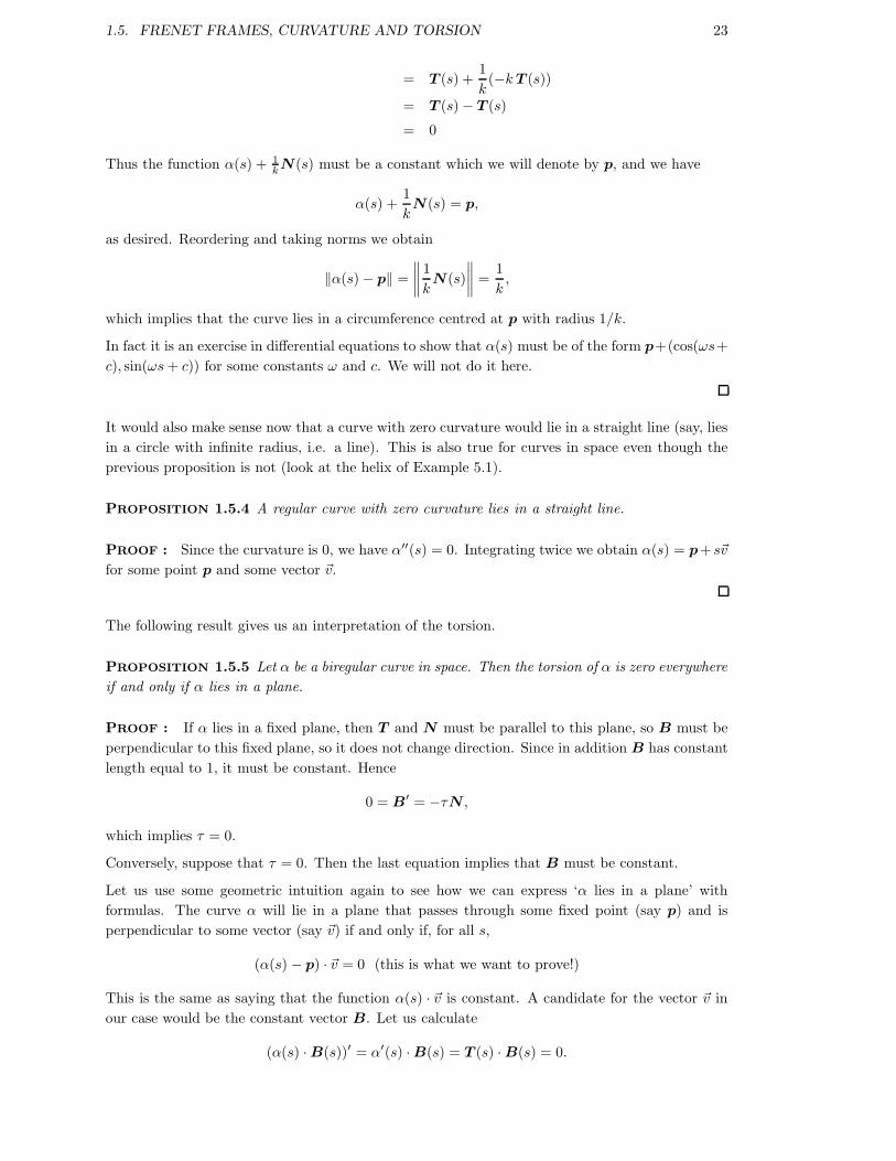
PROPOSITION 1.5.5 Let α be a biregular curve in space. Then the torsion of α is zero everywhere
if and only if α lies in a plane.
PROOF : If α lies in a fixed plane, then T and N must be parallel to this plane, so B must be
perpendicular to this fixed plane, so it does not change direction. Since in addition B has constant
length equal to 1, it must be constant. Hence
0 = B′ = −τN ,
which implies τ = 0.
Conversely, suppose that τ = 0. Then the last equation implies that B must be constant.
Let us use some geometric intuition again to see how we can express ‘α lies in a plane’ with
formulas. The curve α will lie in a plane that passes through some fixed point (say p) and is
perpendicular to some vector (say ~v) if and only if, for all s,
(α(s) − p) · ~v = 0 (this is what we want to prove!)
This is the same as saying that the function α(s) · ~v is constant. A candidate for the vector ~v in
our case would be the constant vector B. Let us calculate
(α(s) · B(s))′ = α′(s) · B(s) = T (s) · B(s) = 0.
24 CHAPTER 1. CURVES
Thus (α(s) · B(s)) is constant. If s0 is some fixed value of s in the domain of α(s), we have
α(s) · B(s) = α(s0) · B(s0)
for all s, and therefore
(α(s) − α(s0)) · B(s) = 0,
which expresses the fact that α lies in the plane passing through α(s0) that is perpendicular to
the (constant) vector B(s).
This proposition gives a geometrical interpretation of the torsion: it is a measure of how much a
curve fails to be in a plane. We give now a more physical interpretation.
Suppose that you are riding in a roller coaster so that your head is always pointing in the direction
of the normal N of the curve described by the roller coaster (this is the safest choice: the centrifugal
force will only push us up or down, not to the sides, so it is more difficult to fall). If you stretch
your arms in a cross then one arm will go up and the other will go down. The speed at which they
move is the torsion.
And a most enlightening view of curvature and torsion is the following.
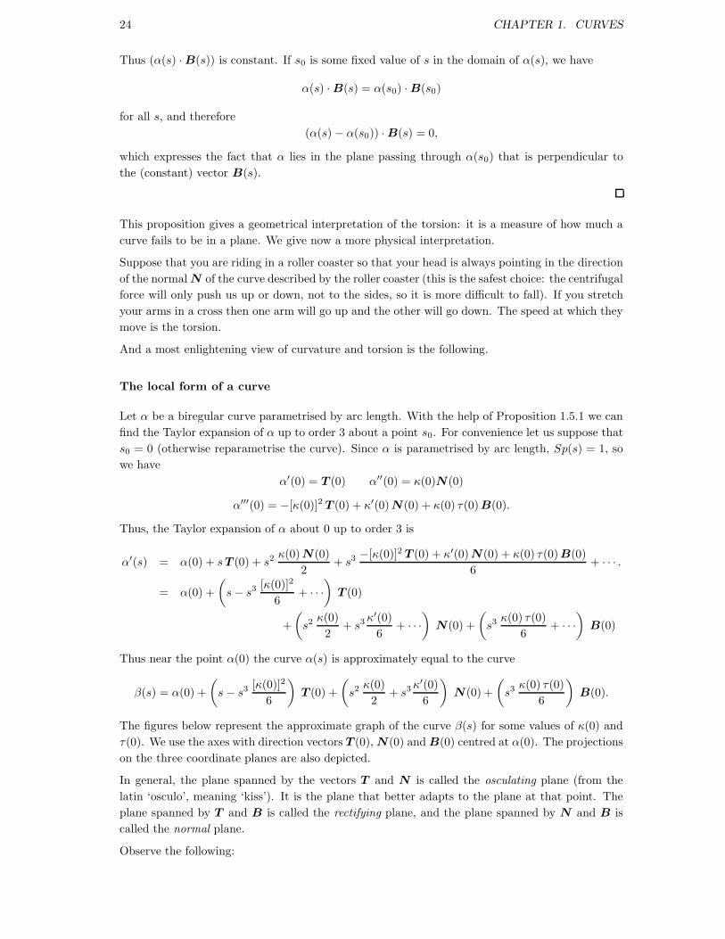
The local form of a curve
Let α be a biregular curve parametrised by arc length. With the help of Proposition 1.5.1 we can
find the Taylor expansion of α up to order 3 about a point s0. For convenience let us suppose that
s0 = 0 (otherwise reparametrise the curve). Since α is parametrised by arc length, Sp(s) = 1, so
we have
α′(0) = T (0) α′′(0) = κ(0)N(0)
α′′′(0) = −[κ(0)]2 T (0) + κ′(0) N(0) + κ(0) τ(0) B(0).
Thus, the Taylor expansion of α about 0 up to order 3 is
α′(s) = α(0) + s T (0) + s2 κ(0) N(0)
2+ s3 −[κ(0)]2 T (0) + κ′(0) N(0) + κ(0) τ(0) B(0)
6+ · · · .
= α(0) +
(
s − s3 [κ(0)]2
6+ · · ·
)
T (0)
+
(
s2 κ(0)
2+ s3 κ′(0)
6+ · · ·
)
N(0) +
(
s3 κ(0) τ(0)
6+ · · ·
)
B(0)
Thus near the point α(0) the curve α(s) is approximately equal to the curve
β(s) = α(0) +
(
s − s3 [κ(0)]2
6
)
T (0) +
(
s2 κ(0)
2+ s3 κ′(0)
6
)
N(0) +
(
s3 κ(0) τ(0)
6
)
B(0).
The figures below represent the approximate graph of the curve β(s) for some values of κ(0) and
τ(0). We use the axes with direction vectors T (0), N(0) and B(0) centred at α(0). The projections
on the three coordinate planes are also depicted.
In general, the plane spanned by the vectors T and N is called the osculating plane (from the
latin ‘osculo’, meaning ‘kiss’). It is the plane that better adapts to the plane at that point. The
plane spanned by T and B is called the rectifying plane, and the plane spanned by N and B is
called the normal plane.
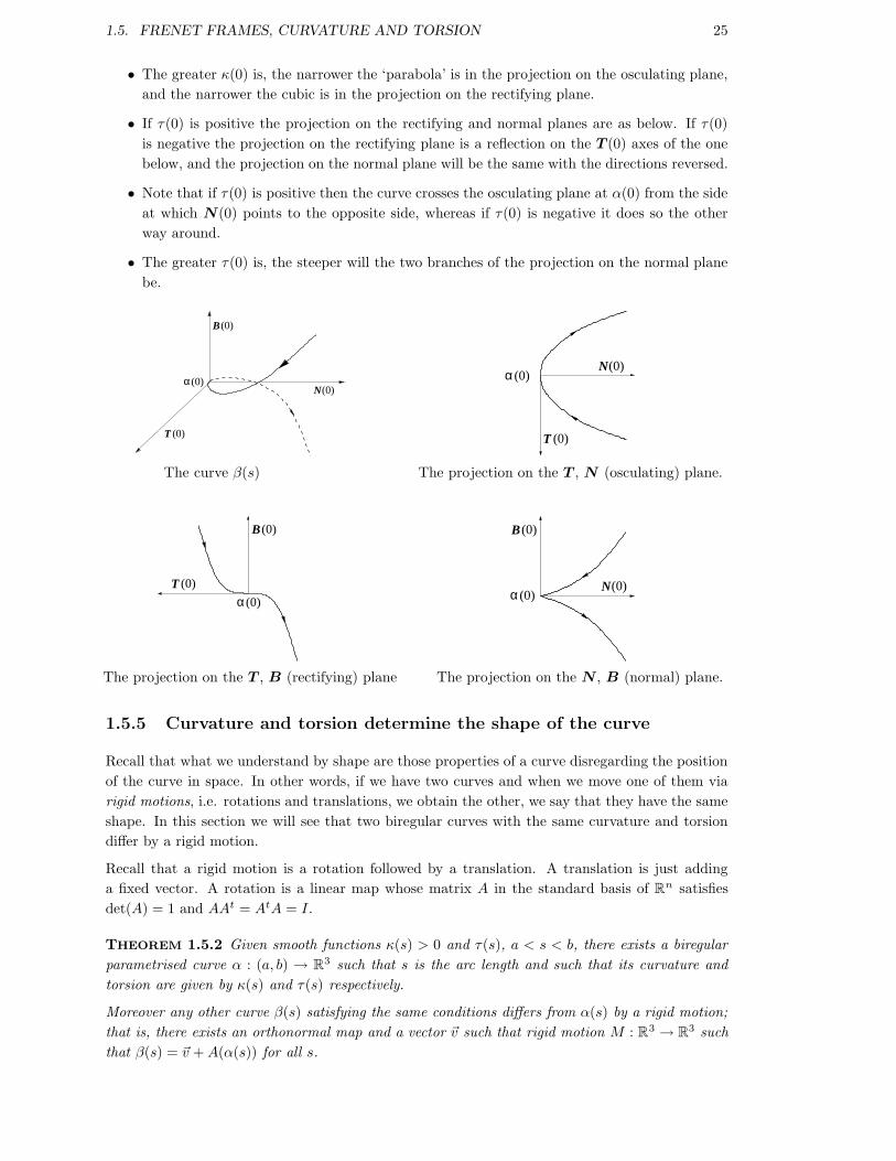
Observe the following:
1.5. FRENET FRAMES, CURVATURE AND TORSION 25
• The greater κ(0) is, the narrower the ‘parabola’ is in the projection on the osculating plane,
and the narrower the cubic is in the projection on the rectifying plane.
• If τ(0) is positive the projection on the rectifying and normal planes are as below. If τ(0)
is negative the projection on the rectifying plane is a reflection on the T (0) axes of the one
below, and the projection on the normal plane will be the same with the directions reversed.
• Note that if τ(0) is positive then the curve crosses the osculating plane at α(0) from the side
at which N(0) points to the opposite side, whereas if τ(0) is negative it does so the other
way around.
• The greater τ(0) is, the steeper will the two branches of the projection on the normal plane
be.
N(0)
B(0)
T (0)
α(0)N(0)
T (0)
α(0)
The curve β(s) The projection on the T , N (osculating) plane.
α(0)
B(0)
T (0)α(0)
N(0)
B(0)
The projection on the T , B (rectifying) plane The projection on the N , B (normal) plane.
1.5.5 Curvature and torsion determine the shape of the curve
Recall that what we understand by shape are those properties of a curve disregarding the position
of the curve in space. In other words, if we have two curves and when we move one of them via
rigid motions, i.e. rotations and translations, we obtain the other, we say that they have the same
shape. In this section we will see that two biregular curves with the same curvature and torsion
differ by a rigid motion.
Recall that a rigid motion is a rotation followed by a translation. A translation is just adding
a fixed vector. A rotation is a linear map whose matrix A in the standard basis of Rn satisfies
det(A) = 1 and AAt = AtA = I .
THEOREM 1.5.2 Given smooth functions κ(s) > 0 and τ(s), a < s < b, there exists a biregular
parametrised curve α : (a, b) → R3 such that s is the arc length and such that its curvature and
torsion are given by κ(s) and τ(s) respectively.
Moreover any other curve β(s) satisfying the same conditions differs from α(s) by a rigid motion;
that is, there exists an orthonormal map and a vector ~v such that rigid motion M : R3 → R
3 such
that β(s) = ~v + A(α(s)) for all s.
26 CHAPTER 1. CURVES
The proof of this theorem needs some important results. First of all we need the following theorem
from ODE that we state without proof.
THEOREM 1.5.3 Let A : (a, b) → Mn×n(R) be a smooth function, where Mn×n(R) denotes the
set of n by n matrices with real entries. Let t0 ∈ (a, b) and x0 ∈ Rn.
Then there exists a unique function x : (a, b) → Rn such that
x′(t) = A(t)x(t) and x(t0) = x0.
Using this theorem we state and prove a refined version of the first half of Theorem 1.5.2.
PROPOSITION 1.5.6 Let κ(s) > 0 and τ(s), a < s < b, be smooth functions. Let s0 ∈ (a, b) be
a fixed number, let p ∈ R3 be a point in R
3 and let {~e1, ~e2, ~e3}, with ~e3 = ~e1 × ~e2, be a positively
oriented orthonormal frame.
Then there exists a unique biregular parametrised curve α : (a, b) → R3 such that α is parametrised
by arc length, such that its curvature and torsion are given by κ(s) and τ(s) respectively, and such
that α(s0) = p, T (s0) = ~e1, N(s0) = ~e2 and B(s0) = ~e3.
PROOF :
Set the following system of differential equations (in R12):
α′(s) = T (s)T ′(s) = κ(s)N(s)N ′(s) = −κ(s)T (s) + τ(s)B(s)B′(s) = −τ(s)N(s)
with the conditions
α(s0) = p
T (s0) = ~e1
N(s0) = ~e2
B(s0) = ~e3
(These equations are just the definition of T and the Frenet-Serret equations.) It can be written
in the form specified in the hypotheses of the last theorem, so this implies that there is a unique
solution satisfying the given condition. It only remains to prove that the functions T , N and B
form the Frenet frame of the curve α(s). The proof of this fact is not trivial.
Suppose that α(s), T (s), N(s) and B(s) are a solution of the system of equations above. Then
the dot products of the vectors T , N and B must implicitly satisfy the following (this is a matter
of applying the product rule in the derivatives of the dot products and using the expression for T ′,
N ′ and B′ above):
(T (s) · T (s))′ = 2κ(s) (T (s) · N(s))(T (s) · N(s))′ = κ(s) (N(s) · N(s)) − κ(s) (T (s) · T (s)) + τ(s) (T (s) · B(s))(T (s) · B(s))′ = τ(s) (T (s) · N(s)) − κ(s) (N(s) · B(s))(N(s) · N(s))′ = −2κ(s) (N(s) · T (s)) + 2τ(s) (N(s) · B(s))(N(s) · B(s))′ = −κ(s) (T (s) · B(s)) − τ(s) (N(s) · N(s)) + τ(s) (B(s) · B(s))(N(s) · N(s))′ = −2τ(s) (N(s) · B(s))
with initial conditons
T (s0) · T (s0) = 1N(s0) · N(s0) = 1B(s0) · B(s0) = 1T (s0) · N(s0) = 0T (s0) · B(s0) = 0N(s0) · B(s0) = 0
1.5. FRENET FRAMES, CURVATURE AND TORSION 27
Note that this is not a system on the vectors T , N and B but on all their possible pairwise dot
products. The previous theorem guarantees that the system has a unique solution. But note that
T (s) · T (s) = 1N(s) · N(s) = 1B(s) · B(s) = 1T (s) · N(s) = 0T (s) · B(s) = 0N(s) · B(s) = 0
is ‘also’ a solution (this needs to be checked - we leave it for the reader). Thus it must be the
solution. Therefore the frame formed by the vectors T , N and B is orthonormal. In addition,
since B has length one and is perpendicular to both T and N , it must be either equal to T × N
or −T × N . It cannot be one of them for some values of the parameter and the other one for
other values because this would contradict continuity of B. Since at s0 we have T × N = B,
we must thus have that this equation is true for all values of the parameter. Therefore the frame
formed by T , N and B must be the Frenet frame for α(s) since it satisfies T = α′, N = T ′/κ
and B = T × N .
Now we are ready to prove the second part of Theorem 1.5.2.
PROOF : Suppose that α(s) and β(s) have the same curvature κ(s) and the same torsion τ(s)
for every s. Let s0 be a point in the domain of α and β, and let {Tα(s0), Nα(s0), Bα(s0)} and
{Tβ(s0), Nβ(s0), Bβ(s0)} be the Frenet frames at the point s0 of α and β, respectively. Let A be
a 3 by 3 orthogonal matrix with determinant 1 that satisfies
A Tα(s0) = Tβ(s0)
A Nα(s0) = Nβ(s0)
A Bα(s0) = Bβ(s0)
(Note that both Frenet frames are orthonormal and positively oriented so such an orthogonal map
must exist—check Chapter 0.) Let us calculate the curvature κ(s) and torsion τ (s) of the curve
α(s) = ~v + A(α(s)), where ~v = β(s0) − A(α(s0)). First we have
α′(s) = DAα(s)(α′(s)) = A(α′(s)),
since the derivative of a linear function is itself, and also
α′′(s) = DAα′(s)(α′′(s)) = A(α′′(s)),
α′′′(s) = DAα′′(s)(α′′′(s)) = A(α′′′(s)).
Let us use the formulas in section 5.3.
κ(s) =‖α′(s) × α′′(s)‖
‖α′(s)‖3
=‖A(α′(s)) × A(α′′(s))‖
‖A(α′(s))‖3
=‖ det(A)A(α′(s) × α′′(s))‖
‖A(α′(s))‖3
=‖α′(s) × α′′(s)‖
‖α′(s)‖3
= κ(s),
28 CHAPTER 1. CURVES
since A preserves norms and has determinant 1 since it is orthonormal.
τ (s) =(α′(s) × α′′(s)) · α′′′(s)
‖α′(s) × α′′(s)‖2
=[A(α′(s)) × A(α′′(s))] · A(α′′′(s))
‖A(α′(s)) × A(α′′(s))‖2
=det(A) ((α′(s) × α′′(s)) · α′′′(s))
‖ det(A) A(α′(s) × α′′(s))‖2
=(α′(s) × α′′(s)) · α′′′(s)
‖α′(s) × α′′(s)‖2
= τ(s)
To finish the proof, note that α(s) and β(s) have the same curvature and torsion, and the same
Frenet frame at the common point β(s0) (note that α(s0) = β(s0)). Then, by the uniqueness part
of the last proposition, they must be the same curve. Hence , writing p = β(s0) − A(α(s0)), we
have
β(s) = ~v + A(α(s)) for all s ∈ (a, b),
so α and β differ by a rigid motion, as claimed.

Chapter 2
Surfaces
2.1 What is a surface?
2.1.1 Regular surfaces and parametrised surfaces
As in the case of curves, we make two definitions of the concept of surface. One of them (regular
surface) emphasizes the fact that a surface, as we think of it, is a set of points. The other
(parametrised surface) emphasizes the parametrization of the surface. While these two concepts
were similar in the case of curves (every regular curve can be covered with a single parametrization,
so it is a parametrised regular curve), they are different for surfaces: a sphere, for example, is a
regular surface, but not a parametrised regular surface.
From now on we specialise for the case of surfaces in R3. For the definitions for surfaces in R
n,
any n, just substitute 3 for n.
DEFINITION 2.1.1 A parametrised surface is a smooth map σ : U ⊂ R2 → R
3, where U is open
in R2. The surface is called regular parametrised surface if the map σ is regular.
The regularity condition is there to guarantee that the image of σ is indeed what we intuitively
understand as a surface (otherwise, taking σ constant—so not regular—we would have that a point
is a surface, which is counterintuitive).
DEFINITION 2.1.2 A regular surface S is a subset of R3 such that for every point p ∈ S there is
an open set V ∈ R3, an open set U ∈ R2 and a map σ : U → S ∩ V ⊂ R
3 satisfying
• σ is a homeomorphism.
• σ is smooth.
• σ is regular.
Each map σ : U → S ∩ V ⊂ R3 of this sort is called
a surface patch or parametrization; σ−1 is often called a chart.
This second definition probably looks complicated.
Let us explain what it means. First let us do a picture.
V Sp
V
σ
UR2
29
30 CHAPTER 2. SURFACES
The situation depicted above is for each p in S. In other words, a surface is some subset of R3
that can be covered by surface patches. Each surface patch looks like a (maybe deformed) piece
of R2.
A set of surface patches covering S is called an atlas.
Think of the surface patches as if they were maps (in the cartographic sense) of parts of the surface,
and an atlas as a collection of all these maps (like an ‘atlas of the world’ but with the surface).
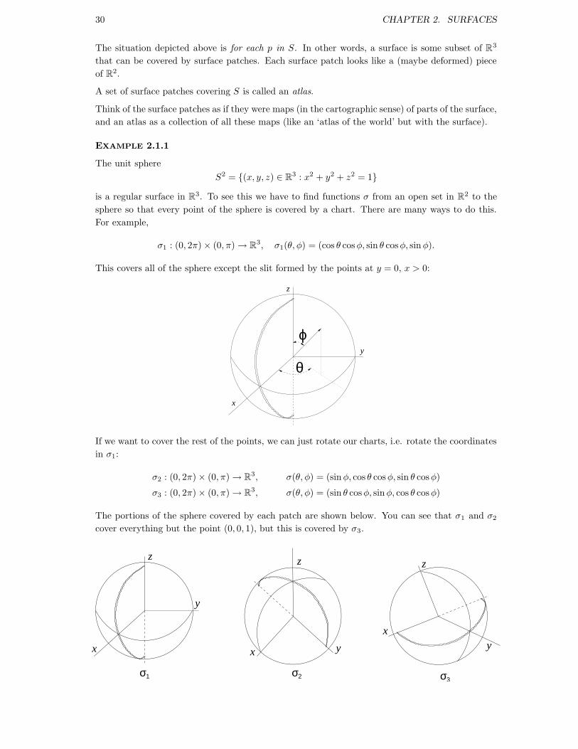
EXAMPLE 2.1.1
The unit sphere
S2 = {(x, y, z) ∈ R3 : x2 + y2 + z2 = 1}
is a regular surface in R3. To see this we have to find functions σ from an open set in R
2 to the
sphere so that every point of the sphere is covered by a chart. There are many ways to do this.
For example,
σ1 : (0, 2π) × (0, π) → R3, σ1(θ, φ) = (cos θ cosφ, sin θ cosφ, sin φ).
This covers all of the sphere except the slit formed by the points at y = 0, x > 0:
ϕ
θ
x
y
z
If we want to cover the rest of the points, we can just rotate our charts, i.e. rotate the coordinates
in σ1:
σ2 : (0, 2π) × (0, π) → R3, σ(θ, φ) = (sin φ, cos θ cosφ, sin θ cosφ)
σ3 : (0, 2π) × (0, π) → R3, σ(θ, φ) = (sin θ cosφ, sin φ, cos θ cosφ)
The portions of the sphere covered by each patch are shown below. You can see that σ1 and σ2
cover everything but the point (0, 0, 1), but this is covered by σ3.
σ1 σ2 σ3
x x
x
y
z z z
y y

2.1. WHAT IS A SURFACE? 31
In the case of curves, all regular curves were parametrised regular curves, or equivalently they
were covered by a single coordinate patch, this is not the case for surfaces. For example, a sphere
cannot be covered by a single coordinate patch (think of wrapping a ball with paper; then when
you try to close it many points of the wrapping will cover very few points of the sphere. At these
points the coordinate patch will not be regular). On the other hand parametrised regular surfaces
with a self intersection will not be regular surfaces (at the self intersection they do not look like a
piece of the plane, as regular surfaces should).
So it may seem that we should treat these two cases separately. However, note that the portion of
a regular surface parametrised by a single patch is a regular parametrised surface, so the study of
local properties of surfaces is essentially the same for both cases.
In any case, in this course we will concentrate our study in regular surfaces, i.e. we will exclude
surfaces with self-intersections.
2.1.2 How to see that something is a surface
It would be very annoying if we had to check all the properties in Definition 1.2 to see that
something is a surface. Fortunately we have some simpler criteria.
PROPOSITION 2.1.1 If f : U ∈ R2 → R is smooth, then the graph of f is a regular surface that
is covered by a single patch.
PROOF :
Recall that the graph of a function f is the set of points of the form {(x, y, f(x, y)) : x, y ∈ U}.So let σ : U → R
3 be defined as σ(u, v) = (u, v, f(u, v)) (we could use x and y as variables but for
some reason it is customary to use u and v). Let us check that σ is an acceptable patch.
First by definition of the graph of f , σ covers all of it, so it is onto. It is also injective since different
(u, v) will give different (u, v, f(u, v)), so σ is bijective.
σ is continuous and smooth because u, v and f(u, v) are. The inverse of σ is just the projection
π(u, v, f(u, v)) = (u, v), which is also continuous.
Finally,
Dσ(u,v) =
1 00 1
fu(u, v) fv(u, v)
,
which has rank 2, and therefore it is regular.
Another useful criterion is
PROPOSITION 2.1.2 Let F : R3 → R be a smooth function. Consider the set S = {(x, y, z) :
F (x, y, z) = 0}. If ∇F 6= 0 at every point of S, then S is a regular surface.
PROOF : (sketch) This is a consequence of the implicit function theorem, that essentially says
that given an equation of the form F (x, y, z) = 0 with F regular then one can always solve for one
of the variables, at least locally. So to fix ideas suppose that we can solve for z, i.e. we can write
F (x, y, z) = 0 ⇐⇒ z = f(x, y).
Then S will be locally the graph of the function f .
Note that we cannot expect all of S to be the graph of a function, as the following example shows.
32 CHAPTER 2. SURFACES
EXAMPLE 2.1.2
Consider F (x, y, z) = x2+y2+z2−1. Then ∇f = (2x, 2y, 2z) which is not zero when F (x, y, z) = 0
(since if x2 + y2 + z2 − 1 = 0 then either x, y or z is not 0). So the set of points where F is 0 is a
regular surface—a sphere as you know—normally denoted as S2.
Let us try to patch S2 with graphs of functions:
• The graph of z =√
1 − x2 − y2 covers the top open hemisphere.
• The graph of z = −√
1 − x2 − y2 covers the bottom open hemisphere.
• The graph of y =√
1 − x2 − z2 covers the right open hemisphere.
• The graph of y = −√
1 − x2 − z2 covers the left open hemisphere.
• The graph of x =√
1 − y2 − z2 covers the front open hemisphere.
• The graph of x = −√
1 − y2 − z2 covers the back open hemisphere.
These six patches cover all of S2. Note that neither of these patches can only be defined when
whatever is inside the square root is greater than 0, and cannot be extended any further.
EXAMPLE 2.1.3
Surfaces of revolution: consider the surface M obtained by rotating a curve (f(v), 0, g(v)),
v ∈ (a, b) lying in the xz-plane about the z-axes. To guarantee regularity of M we assume that
the curve is regular and that f(v) > 0 for all v.
A patch for M will be
σ(u, v) = (f(v) cosu, f(v) sin u, g(v)), 0 < u < 2π, a < v < b.
σ covers all of M except for the slit corresponding to the original curve (f(v), 0, g(v)). In order to
cover this slit let
τ(u, v) = (f(v) cosu, f(v) sinu, g(v)), −π < u < π, a < v < b.
Then σ and τ together cover all of M .
Note that σ is regular (for τ is the same computation):
σu = (−f(v) sin u, f(v) cosu, 0) and σv = (f ′(v) cos u, f ′(v) sin u, g′(v)).
σu × σv = (f(v)g′(v) cosu, f(v)g′(v) sin u,−f(v)f ′(v)),
which is never 0 since f(v) > 0 and f ′(v) or g′(v) cannot both be 0 (the original curve is regular).
Of course we could have started with a curve in any vertical plane instead of the xz-plane; it works
the same way. We could also have rotated a curve about any of the other axes, provided that the
original curve is chosen accordingly.
2.2. THE TANGENT PLANE 33
2.2 The tangent plane
DEFINITION 2.2.1 Let M be a regular surface and p ∈ M . The tangent plane of M at p is
TpM = {α′(t0) where α : (a, b) → M smooth curve and α(t0) = p}
In other words, TpM is the set of all possible tangent vectors to curves in M at the point p.
LEMMA 2.2.1 Let σ : U ⊂ R2 → M be a surface patch with p = σ(u0, v0). Then
TpM = span {σu(u0, v0), σv(u0, v0)}
PROOF : First we show that TpM ⊃ span {σu(u0, v0), σv(u0, v0)}. Consider the curve
α(t) = σ(u0 + at, v0 + bt),
where a and b are arbitrary numbers. Now, α(0) = σ(u0, v0) = p, so α′(0) ∈ TpM . However, the
chain rule gives
α′(0) =∂σ
∂u(u0, v0) a +
∂σ
∂v(u0, v0) b = aσu(u0, v0) + bσv(u0, v0),
proving that TpM ⊃ span {σu(u0, v0), σv(u0, v0)}.Now we prove that TpM ⊂ span {σu(u0, v0), σv(u0, v0)}. If α : (a, b) → M is a curve with
α(t0) = p then for t in some subinterval (a′, b′) the curve will lie in σ(U), and hence we can write
α(t) = σ(β(t)) for some curve β(β1(t), β2(t)) : (a′, b′) → U ⊂ R2. (We take as given the fact that
β is smooth; this is a consequence of the inverse function theorem.) Then, using the chain rule,
α′(t0) = β′1(t0) σu(u0, v0) + β′
2(t0) σv(u0, v0) ∈ span {σu(u0, v0), σv(u0, v0)}.
REMARK 2.2.1
Since TpM is the span of two vectors, it must be a vector subspace of R3.
Strictly speaking, TpM should be defined as the space of pairs (p, α′(t0)) ∈ R3 × R
3, where
α : (a, b) → M is a curve such that α(t0) = p. The vector addition and multiplication by scalars
in TpM would be then defined as λ(p,~v) + (p, ~w) = (p, λ~v + ~w). We will not use this formalism to
avoid complication with notation.
However, it is always convenient to think of TpM as the vector space specified in the definition
but ‘anchored at the point p’. Geometrically we could think of it as the plane that is ‘tangent’ to
M at p, but then this plane would not pass, in general, through the 0 of R3, so it would not be a
vector space. So think of TpM as a vector space, again, ‘anchored’ at p, or if you want, with a tag
indicating that it is tangent at the point p.
EXAMPLE 2.2.1 The tangent space to M parametrised by σ(u, v) = (u, v, u2 + v2) at the point
p = (1, 1, 2) = σ(1, 1) is the subspace of R3 given by
{a σu(1, 1) + b σv(1, 1)} =
a
102
+ b
012
.

34 CHAPTER 2. SURFACES
2.3 Functions on surfaces
DEFINITION 2.3.1 Let M and N be a regular surfaces. A function f : M → Rn is said to be
differentiable if f ◦ σ : U → Rn is differentiable for every surface patch σ : U → M of M .
A function f : M → N ⊂ R3 is differentiable (as a function from M to N) if it is differentiable as
a function from M to R3.
Given charts σ : U → M and τ : V → N the expression
τ−1 ◦ f ◦ σ : U → V
(wherever it is defined) is called ‘local expression of f in the patches σ to τ ’. It turns out that f is
differentiable if and only if the local expression in any patches is differentiable.
σfτ−1
σ τ
f
M N
(U)σ
τ(V)
VU
2.4 Vector fields
DEFINITION 2.4.1 Let M ⊂ R3 be a regular surface. A vector field in M is a map
X : M → R3
p → Xp
where we think of the value of X at a point p as a vector in R3 ‘anchored’ at p (whatever this may
mean. . . ). To emphasize this fact we normally write Xp instead of X(p) for the value of X at p
(although we will use both notations).
A vector field is tangent if Xp ∈ TpM ∀p, and normal if Xp ⊥ TpM ∀p.
REMARK 2.4.1
Let TR3 be the set of pairs (p, v) ⊂ R
3 × R3 with addition and multiplication by scalars defined
by λ(p, v) + (p, w) = (p, λv + w). Then, strictly speaking, a vector field is a map from M to TR3
that satisfies X(p) = (p, Xp).
This view of vector fields is certainly more correct but for our present purposes would only com-
plicate matters, so we will think of vector fields just as maps from M to R3.
2.5. NORMAL VECTOR FIELDS AND ORIENTABILITY 35
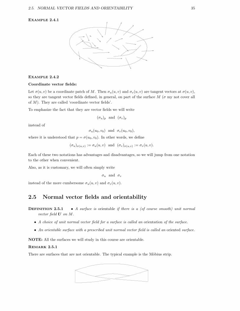
EXAMPLE 2.4.1
EXAMPLE 2.4.2
Coordinate vector fields:
Let σ(u, v) be a coordinate patch of M . Then σu(u, v) and σv(u, v) are tangent vectors at σ(u, v),
so they are tangent vector fields defined, in general, on part of the surface M (σ my not cover all
of M). They are called ‘coordinate vector fields’.
To emphasize the fact that they are vector fields we will write
(σu)p and (σv)p
instead of
σu(u0, v0) and σv(u0, v0),
where it is understood that p = σ(u0, v0). In other words, we define
(σu)σ(u,v) := σu(u, v) and (σv)σ(u,v) := σv(u, v).
Each of these two notations has advantages and disadvantages, so we will jump from one notation
to the other when convenient.
Also, as it is customary, we will often simply write
σu and σv
instead of the more cumbersome σu(u, v) and σv(u, v).
2.5 Normal vector fields and orientability
DEFINITION 2.5.1 • A surface is orientable if there is a (of course smooth) unit normal
vector field U on M .
• A choice of unit normal vector field for a surface is called an orientation of the surface.
• An orientable surface with a prescribed unit normal vector field is called an oriented surface.
NOTE: All the surfaces we will study in this course are orientable.
REMARK 2.5.1
There are surfaces that are not orientable. The typical example is the Mobius strip.

36 CHAPTER 2. SURFACES
REMARK 2.5.2
Given a local patch σ on an oriented surface M , we have
either Uσ(u, v) =σu × σv
‖σu × σv‖or Uσ(u, v) = − σu × σv
‖σu × σv‖.
EXAMPLE 2.5.1
For the surface parametrised by σ(u, v) = (u, v, u2 + v2), σu = (1, 0, 2u), σv = (0, 1, 2v), so
σu × σv = (−2u,−2v, 1) and therefore
Uσ(u,v) =(−2u,−2v, 1)√4u2 + 4v2 + 1
or Uσ(u,v) =(2u, 2v,−1)√4u2 + 4v2 + 1
.
REMARK 2.5.3
For the rest of the course many things will depend on the choice of the unit normal vector. Both
choices of normal are perfectly admissible and many of the quantities we will define using U will
not be invariant under a change of orientation, so before an orientation is chosen there will be a
degree of ambiguity in our definitions.
2.6 Differentiation on surfaces
To be able to study the shape of surfaces we will have to differentiate functions and vector fields
that are only defined on a surface, and not on an open set of R3. In this and previous courses
you have seen the definition of derivative for functions defined on an open set in Rn, but not for
functions defined in surfaces. Hence we have to define the derivative on surfaces.
The derivative measures the rate of change of some quantity when another quantity changes. Note
that in a surface we have many directions in which to measure these rates of change, so we need to
define derivatives with respect to a direction (actually with respect to a vector). These are called
directional derivatives.
DEFINITION 2.6.1 Let M be a regular surface, f : M → Rn a function and X : M → R
3 a
vector field.
The directional derivative of f or X with respect to ~w ∈ TpM is defined, respectively, as
D~wf(p) =d
dtt0
f(α(t)) or D~wXp =d
dtt0
X(α(t)),
where α : (a, b) → M is a curve such that α(t0) = p and α′(t0) = ~w.
(Note that the definition for f and X is exactly the same; a distinction is made just because of
the ‘vector field character’ of X : Xp is thought of as ‘anchored’ at p.)
How can we calculate these objects in a painless way?
PROPOSITION 2.6.1 Let f : M ⊂ R3 → R
n be a function and X be a vector field in M .
• If f is defined not only on M but on an open subset of R3 containing M , then
D~wf(p) = Dfp(~w),
where Dfp is the usual derivative of f at p.
2.6. DIFFERENTIATION ON SURFACES 37
• If ~w = a(σu)p + b(σv)p ∈ TpM then
D~wXp = a∂(X ◦ σ)
∂u(u0,v0)
+ b∂(X ◦ σ)
∂v(u0,v0)
,
where (u0, v0) are such that p = σ(u0, v0). Note that in particular,
DσuXp =
∂(X ◦ σ)
∂u(u0,v0)
and DσvXp =
∂(X ◦ σ)
∂u(u0,v0)
.
PROOF :
• Let α : (a, b) → M be a smooth curve with α(t0) = p, α′(t0) = ~w. Using the chain rule,
D~wf(p) =d
dtt0
f(α(t)) = Dfα(t0)(α′(t0)) = Dfp(~w).
• Consider the curve α(t) = σ(u0 + at, v0 + bt). Then α(0) = σ(u0, v0) = p and α′(0) =
a(σu)p + b(σv)p = ~w. Hence, using the chain rule,
D~wXp =dX ◦ σ(u0 + at, v0 + bt)
dtt=0
=∂(X ◦ σ)
∂uα(0)
d(u0 + at)
dt+
∂(X ◦ σ)
∂uα(0)
d(v0 + bt)
dt
= a∂(X ◦ σ)
∂u(u0,v0)
+ b∂(X ◦ σ)
∂v(u0,v0)
.
Some properties of the directional derivative
PROPOSITION 2.6.2 The directional derivative satisfies
• For ~w1, ~w2 ∈ TpM ,
Da1 ~w1+a2 ~w2Xp = a1D~w1
Xp + a2D~w2Xp.
• For X and Y vector fields,
D~w(X · Y )(p) = (D~wXp) · Yp + Xp · (D~wYp).
This also holds if we substitute · with ×.
• If σ is a surface patch about p, then
(Dσuσv)p = (Dσv
σu)p.
PROOF :
• Write ~w1 and ~w2 in the basis given by σu and σv , collect terms and apply the last statement
of the previous proposition.
• If α : (a, b) → M is such that α(t0) = p and α′(t0) = ~w then
D~w(X · Y )(p) =X(α(t)) · Y (α(t))
dtt0
=
(
X(α(t))
dtt0
)
· Y + X ·(
Y (α(t))
dtt0
)
= (D~wXp) · Yp + Xp · (D~wYp).
The proof for × is the same.

38 CHAPTER 2. SURFACES
• Use the last statement of the previous proposition:
(Dσuσv)p =
∂(σv)σ(u,v)
∂u= σuv = σvu =
∂(σu)σ(u,v)
∂v= (Dσv
σu)p.
Chapter 3
Local geometry of surfaces
Now we have the tools from calculus we need in order to start studying the shape of surfaces.
For curves we differentiated the tangent vector in order to obtain the curvature. We could do the
same in surfaces, except that we do not quite have a tangent vector but a tangent plane. Now,
each tangent plane is completely characterised by the unit normal vector, so our strategy will be
to differentiate the normal in order to obtain information about the shape of a surface.
3.1 The shape operator
DEFINITION 3.1.1 Let M be an regular oriented surface with unit normal U . The shape operator
on M is the linear transformation
Sp : TpM → TpM
defined by
Sp(~w) = −D~wUp.
REMARK 3.1.1
Note that S is actually something like a ‘field’ of linear transformations: S gives a linear map Sp
for each p ∈ M .
Observe also that there is no reason a priori that −D ~wUp will actually lie in TpM . We prove this
in the following lemma.
LEMMA 3.1.1 Let M be an oriented surface and p ∈ M . Then we have
• Sp is well defined as a map into TpM in the sense that Sp(~w) ∈ TpM .
• Sp is linear.
• Sp is symmetric, in the sense that Sp(~v) · ~w = ~v · Sp(~w).
PROOF :
• Since U · U = 1, we have 0 = D~w(U · U)(p) = 2(D~wUp) · Up. Therefore SpD~wUp is
perpendicular to Up so it lies in TpM .
• Using the properties of the directional derivative, we have Sp(a~v + b~w) = −Da~v+b~wU =
−− aD~vU − bD~wU = aSp(~v) + bSp(~w).
39
40 CHAPTER 3. LOCAL GEOMETRY OF SURFACES
• Let σ be a surface patch about p. Then we can write ~v = a1(σu)p + a2(σv)p and ~w =
b1(σu)p + b2(σv)p. Thus we have (we remove the subscript p in σu and σv for easier reading)
Sp(~v) · ~w = Sp(a1σu + a2σv) · (b1σu + b2σv)
= (a1Sp(σu) + a2Sp(σv)) · (b1σu + b2σv)
= a1b1(Sp(σu) · σu) + a1b2(Sp(σu) · σv) + a2b1(Sp(σv) · σu)
+a2b2(Sp(σv) · σv).
Similarly,
~v · Sp(~w) = a1b1(Sp(σu) · σu) + a1b2(Sp(σv) · σu) + a2b1(Sp(σu) · σv)
+a2b2(Sp(σv) · σv).
Comparing the two expressions it becomes clear that it suffices to show that Sp(σv) · σu =
Sp(σu) · σv . Now, observe that since (σu · U) = 0, we have
0 = Dσu(σv · U)(p) = Dσu
σv · Up + σv · DσuUp = σuv · U + σv · Dσu
Up.
Similarly,
0 = Dσv(σu · U)(p) = σvu · U + σu · Dσv
Up.
Since σuv = σvu we finally have
Sp(σu) · σv = −σv · DσuU = σuv · U = −σu · Dσv
Up = Sp(σv) · σu.
NOTATION: Given a surface patch σ, the matrix expression of Sp in the basis {(σu)p, (σv)p}will be denoted by [Sp]σ .
DEFINITION 3.1.2 The symmetric bilinear function
IIp : TpM × TpM → R
defined by
IIp(~v, ~w) = Sp(~v) · ~w
is called the second fundamental form.
It is clear by the last statement of the last proposition that IIp is symmetric in the sense that
II(~v, ~w) = II(~w,~v).
LEMMA 3.1.2 Let σ be a surface patch about p. Then
IIp(a1σu + a2σv , b1σu + b2σv) = ( a1 a2 )
(
e ff g
)(
b1
b2
)
,
where
e = σuu · Up f = σuv · Up g = σvv · Up.
PROOF :
By bilinearity we have
IIp(a1σu + a2σv , b1σu + b2σv) = a1b1 II(σu, σu) + (a1b2 + a2b1) II(σu, σv) + a2b2 II(σv , σv),
3.1. THE SHAPE OPERATOR 41
and from the proof of Lemma 3.1.1 we know that
II(σu, σu) = σuu · Up II(σv , σu) = σuv · Up II(σv , σv) = σvv · Up.
so the only thing that remains to be checked is that
a1b1 e + (a1b2 + a2b1) f + a2b2 g = ( a1 a2 )
(
e ff g
)(
b1
b2
)
,
but this is straightforward.
NOTATION: For a surface patch σ, we will use the notation
[IIp]σ =
(
e ff g
)
.
(Note that the coefficients e, f, g certainly depend on the surface patch chosen.)
What is the relation between [Sp]σ and the matrix [IIp]σ? We need to make another very important
definition that will also be very important when we talk about length and area in a surface.
DEFINITION 3.1.3 The symmetric bilinear function
Ip : TpM × TpM → R
defined by
Ip(~v, ~w) = ~v · ~w
is called the first fundamental form.
LEMMA 3.1.3 Let σ be a surface patch about p. Then
Ip(a1σu + a2σv , b1σu + b2σv) = ( a1 a2 )
(
E FF G
)(
b1
b2
)
,
where
E = σu · σu F = σu · σv G = σv · σv .
PROOF :
By bilinearity we have
Ip(a1σu + a2σv, b1σu + b2σv) = a1b1 (σu · σu) + (a1b2 + a2b1) (σu · σv) + a2b2 (σv · σv),
so the result follows.
REMARK 3.1.2
It may look strange to give a new name and a new symbol to our good old dot product. The
reason for this is that the dot product is defined in all of R3, whereas the first fundamental form
is defined only on the tangent planes of the surface. So in a way is the gadget we would use if we
lived in the surface without knowing we actually lived in R3. We will see more of this later.
NOTATION: For a surface patch σ, we will use the notation
[Ip]σ =
(
E FF G
)
.
(Note that the coefficients E, F, G certainly depend on the surface patch chosen.)
42 CHAPTER 3. LOCAL GEOMETRY OF SURFACES
PROPOSITION 3.1.1 For σ a surface patch about p we have
[IIp]σ = [Ip]σ [Sp]σ .
PROOF :
Let ~v = a1σu + a2σv and ~w = b1σu + b2σv . Then, by definition,
IIp(~w,~v) = ~w · Sp(~v) = Ip(~w, Sp(~v)).
In terms of matrices this can be written as
( w1 w2 ) [IIp]σ
(
v1
v2
)
= ( w1 w2 ) [Ip]σ [Sp]σ
(
v1
v2
)
.
Since the last equality holds for all w1, w2, v1, v2, the result follows.
REMARK 3.1.3
The previous proposition is very useful for calculations: finding [Ip]σ and [IIp]σ is a routine matter,
whereas finding [Sp]σ directly can be messier. So we will often use the formula
[Sp]σ = [Ip]−1σ [IIp]σ .
3.2 Curvature
It is maybe intuitively clear that the shape operator gives us a lot of information about the shape
of a surface, as it says how the normal moves as we move along the surface. But Sp is a linear
operator, and we would like to have some numbers that summarise the information that Sp may
give. Certainly the matrix expression for Sp in a patch σ does not do the job since Sp does not
depend on σ but [Sp]σ does, as the matrix of a linear transformation depends on the basis chosen.
However, neither the determinant or the trace depend on the basis chosen, and furthermore they
determine Sp completely. The eigenvalues and eigenvectors of Sp are also independent of any basis
chosen. This motivates the following definitions.
DEFINITION 3.2.1 Let M be an oriented regular surface with shape operator S.
• The Gaussian curvature of M at p is defined by
K(p) = det Sp.
• The mean curvature of M at p is defined by
H(p) =Trace(Sp)
2.
• The principal curvatures at p are the eigenvalues of Sp.
• The principal directions at p are the eigenvectors of Sp.
• The asymptotic directions are the vectors ~v ∈ TpM such that IIp(~v,~v) = 0.
REMARK 3.2.1

3.2. CURVATURE 43
• The linear transformation Sp can be diagonalised because it is symmetric. Furthermore,
there is always an orthonormal basis of eigenvectors. This is a standard result in linear
algebra.
• We therefore have that, if the principal curvatures are different, then the principal direc-
tions are always perpendicular.
• If the principal curvatures at p are equal then every vector in TpM will be a principal
direction. So in particular we could choose two perpendicular principal directions.
Before going into calculating all these quantities in a concrete example, let us derive some properties
and formulas for the objects we just defined.
The following is a standard result in linear algebra.
LEMMA 3.2.1 Let ~w ∈ TpM such that ~w · ~w = 1 (or Ip(~w, ~w) = 1—it is the same thing). Let k1
and k2 denote the principal curvatures at p and assume that k2 ≤ k1. Then
k2 ≤ II(~w, ~w) ≤ k1.
PROOF :
Let {~v1, ~v2} be an orthonormal basis of eigenvectors of Sp so that ~v1 has eigenvalue k1 and ~v2 has
eigenvalue k2. We can then write ~w = a~v1 + b ~v2 for some coefficients a, b satisfying a2 + b2 = 1
(since ~w · ~w = 1). Then, by bilinearity and using the fact that Sp(~v1) = k1 ~v1 and Sp(~v2) = k2 ~v2,
we have
IIp(~w, ~w) = a2 Sp(~v1) · ~v1 + 2ab Sp(~v1) · ~v2 + b2 Sp(~v2) · ~v2
= a2k1~v1 · ~v1 + 2abk1~v1 · ~v2 + b2k2~v2 · ~v2
= k1a2 + k2b
2.
Now, since k2 ≤ k1,
k2 = k2(a2 + b2) = k2a
2 + k2b2 ≤ k1a
2 + k2b2 ≤ k1a
2 + k1b2 = k1(a
2 + b2) = k1,
as desired.
PROPOSITION 3.2.1 (Some formulas)
• If k1 and k2 are the principal curvatures then K(p) = k1k2 and H(p) = (k1 + k2)/2.
• If K and H are the Gaussian and mean curvatures, respectively, then the principal curvatures
are given by H ±√
H2 − K.
• If σ is a surface patch and [Ip]σ =
(
E FF G
)
and [IIp]σ =
(
e ff g
)
then
K(p) =eg − f2
EG − F 2and H(p) =
Trace(Sp)
2=
Ge + Eg − 2Ff
2(EG − F 2).
PROOF :
• In a basis given by principal directions (i.e. eigenvectors of Sp), the matrix of Sp has the
form
(
k1 00 k2
)
, so the result follows.

44 CHAPTER 3. LOCAL GEOMETRY OF SURFACES
• Solve the system of equations given by K = k1k2 and H = (k1 + k2)/2: multiply H by 2k1
to obtain 2Hk1 = k21 + k1k2 = k2
1 + K. Thus k21 − 2Hk1 + K = 0, so completing the square
we get (k1 − H)2 + K = H2, and the result follows.
• Since [Sp]σ = [Ip]−1σ [II]σ, we have K(p) = det([Sp]σ) = det([Ip]
−1σ ) det([II]σ) = (eg −
f2)/(EF − G2).
To find the formula for H , we have
[Sp]σ = [Ip]−1σ [IIp]σ
=
(
E FF G
)−1(e ff g
)
=1
EG − F 2
(
G −F−F E
)(
e ff g
)
=1
EG − F 2
(
Ge − Ff Gf − FgEf − Fe Eg − Ff
)
.
Therefore
H(p) =Trace(Sp)
2=
Ge + Eg − 2Ff
2(EG − F 2).
EXAMPLE 3.2.1
Let us calculate all these objects for the torus of external radius R and internal radius r, with
R > r.
Recall that a patch for the torus that covers most of it is
σ(u, v) = ((R + r cos v) cosu, (R + r cos v) sin u, r sin v), 0 < u, v < 2π.
We have
σu = (R + r cos v)(− sin u, cosu, 0) σv = (−r sin v cosu,−r sin v sin u, r cos v)
σuu = (R + r cos v)(− cosu,− sinu, 0) σuv = (r sin v sinu,−r sin v cosu, 0)
σvv = (−r cos v cosu,−r cos v sin u,−r sin v).
Therefore a choice of normal unit vector is
U =σu × σv
‖σu × σv‖=
r(R + r cos v)(cosu cos v, sin u cos v, sin v)
r(R + r cos v)= (cosu cos v, sin u cos v, sin v).
Denoting by p a generic point σ(u, v) we have
Sp(σu) = −DσuU = −∂U
∂u= (sin u cos v,− cosu cos v, 0) =
− cos v
R + r cos vσu
Sp(σv) = −DσvU = −∂U
∂v= (sin v cosu, sin v sin u,− cos v) =
−σv
r.
Therefore the matrix expression of Sp in the basis {σu, σv} is
[Sp]σ =
− cos v
R + r cos v0
0−1
r
.
Therefore we have
K(p) =cos v
r(R + r cos v)H(p) =
− cos v
2(R + r cos v)+
−1
2r.

3.3. LENGTH AND AREA 45
Since [Sp]σ is already diagonalised, the principal curvatures are
− cos v
2(R + r cos v)with principal direction σu and
−1
2rwith principal direction σv.
Now we calculate [Ip]σ . We have E = σu ·σu = (R+r cos v)2, F = σu ·σv = 0 and G = σv ·σv = r2.
Therefore
[Ip]σ =
(
(R + r cos v)2 00 r2
)
.
And now we find [IIp]σ. We have e = σuu · U = −(R + r cos v) cos v, f = σuv · U = 0 and
g = σvv · U = −r. Therefore
[IIp]σ =
(
−(R + r cos v) cos v 00 −r
)
.
Note that the formula [Ip]σ [Sp]σ = [II]σ is clearly satisfied.
Finally we find the asymptotic directions. Let ~w = aσu + bσv . Then
II(~w, ~w) = ( a b )
(
−(R + r cos v) cos v 00 −r
) (
ab
)
= −a2(R + r cos v) cos v − b2r.
Therefore we have to solve the equation (R + r cos v) cos va2 + rb2 = 0. This has solutions only
when (R + r cos v) cos v < 0, i.e. when cos v ≤ 0, which means that π ≤ v ≤ 3π/2. In this case,
b = ±a√
−(R + r cos v) cos v/r. Therefore the asymptotic directions are
σu ±√
−(R + r cos v) cos v/r σv .
So far we have only done the calculations without further interpretation of the quantities we obtain.
We will do this in due course, but first we need to introduce some more concepts.
3.3 Length and area
Suppose that you are a 2-dimensional being living in a 2-dimensional surface M in R3. First of all,
there is no apparent way that you could know that you live in a space of higher than 2 dimensions.
All your study of your universe would be based in measurements made in the surface where you
live. How much will you be able to know about your world?
Since we are (only!) 3-dimensional beings, we can hopefully help these ‘poor’ creatures. They can
certainly measure angles and lengths on the surface, so they do know the first fundamental form I
at each point p of their world. In fact this is why it is called ‘first fundamental form’: it is exactly
what you can measure if you are a 2D living in the surface. However they do not know that this
very fundamental form actually comes from a dot product in a space of 3 dimensions.
It is clear that these 2D beings can measure lengths of curves: if α is a curve in the surface, you
just have to integrate√
I(α′(t), α′(t)).
Now, can they measure area? Yes: break the surface in small rectangles, measure the lengths of
the sides of each rectangle, multiply the lengths and add up over all the rectangles. What is an
analytic formula for this?
Recall the following definition.
DEFINITION 3.3.1 Let M be a surface and let σ : U → M be a surface patch. Then
Area(σ(U)) =
∫∫
U
‖σu × σv‖ dv du.

46 CHAPTER 3. LOCAL GEOMETRY OF SURFACES
REMARK 3.3.1 If M is covered by a single surface patch σ except maybe for some small subsets
of M (such as curves in the surface) then Area(M) = Area(σ(U)), so the previous definition
applies.
The interesting fact is that area is independent of parametrization, and in fact we can find a
formula in terms of the first fundamental form only:
PROPOSITION 3.3.1 Let σ : U → M be a surface patch. Then
‖σu × σv‖ =√
det([I]σ).
Therefore, using E, F and G to denote the entries of the matrix [I]σ as usual,
Area(σ(U)) =
∫∫
U
√
EG − F 2 dv du.
PROOF :
Recall the formula (~u× ~v)× ~w = (~u · ~w)~v − (~v · ~w) ~u and the formula (~u× ~v) · ~w = (~w × ~u) · ~v. We
have
(σu × σv) · (σu × σv) = ((σu × σv) × σu) · σv = ((σu · σu) σv − (σu · σv) σu) · σv
= (σu · σu)(σv · σv) − (σu · σv)(σu · σv) = EG − F 2.
3.4 Curves in surfaces
We continue with our discussion of two dimensional beings in M . They can certainly measure
velocity. They can also measure acceleration, but they only feel those components of acceleration
that lie in their 2 dimensional world. In other words, 2D’s do not feel any components of acceler-
ation that are normal to the surface, they do not exist for them. We know they do exist, but let
us see what the 2D’s would measure as acceleration.
DEFINITION 3.4.1 Let α(t) be a regular curve in an oriented regular surface M with normal
U . Let T (t) and N(t) be the tangent and normal vectors of α and let κ(t) be its curvature. The
function
κn(t) = κ(t) N(t) · Uα(t)
is called the normal curvature of the curve α in M , and the function
κg(t) = κ(t) N(t) · (Uα(t) × T (t))
is called the geodesic curvature of the curve α in M .
PROPOSITION 3.4.1
κ(t)N(t) = κn(t) Uα(t) + κg(t) (Uα(t) × T (t)).
PROOF : Let p = α(t) and denote T (t) simply by T , etc. Note that the vectors U , T and U ×T
form an orthonormal basis (U and T are perpendicular because T ∈ TpM and U is perpendicular
to TpM). Note that U × T ∈ TpM since it is perpendicular to U .
Since N · T = 0, we have
κN = (κN · T ) T + (κN · U) U + (κN · (U × T )) U × T = κnU + κg(U × T ).
3.4. CURVES IN SURFACES 47
COROLLARY 3.4.1
κ2 = κ2n + κ2
g .
PROOF :
Clear since {U , T , U × T } form an orthonormal basis.
REMARK 3.4.1
Suppose that a 2D inhabitant of M rides her motorcycle at constant speed 1 along some curve in
M . What centrifugal forces will he feel?
We can parametrise this movement by a curve α parametrised by arc length. We then have
α′′(s) = κ(s)N(s) = κn(s) Uα(s) + κg(s) (Uα(s) × T (s)).
However, 2D inhabitants of M do not feel normal directions because the normal is in an extra
dimension they do not comprehend. Therefore they will never feel the normal component of the
centripetal acceleration κnU ; they will only feel the tangent component κg(U × T ).
In other words:
• κn is the normal component of acceleration, not felt by 2D’s living in the surface.
• κg is the tangent component of acceleration, felt by 2D’s living in the surface.
In particular, a curve in M will be the equivalent of a straight line if it has no acceleration at all
as measured from the point of view of the surface, i.e. if κg = 0.
In order to relate these concepts with the principal curvatures we need the following very important
fact.
PROPOSITION 3.4.2 Let α be a regular curve in an oriented surface M with normal U . Then
the normal curvature of α in M is given by
κn(t) = IIα(t)(T (t), T (t)),
where T (t) is the tangent vector to α.
PROOF :
Since α′(t) ∈ Tα(t)M , α′(t) · Uα(t) = 0. Differentiating and applying the definition of directional
derivative for U we obtain
α′′(t) · Uα(t) + α′(t) · Dα′(t)Uα(t) = 0.
Note that by definition −α′(t) · Dα′(t)Uα(t) = α′(t) · Sα(t)(α′(t)) = IIα(t)(α
′(t), α′(t)).
Recall that we have
α′′(t) = Sp′(t)T (t) + [Sp(t)]2κ(t)N(t).
Since T · U = 0 we have
α′′(t) · Uα(t) = [Sp(t)]2 κ(t) N(t) · Uα(t),
and therefore, since Sp(t) = ‖α′(t)‖ and IIp is bilinear,
κn(t) =IIα(t)(α
′(t), α′(t))
[Sp(t)]2= IIα(t)
(
α(t)
‖α(t)‖ ,α(t)
‖α(t)‖
)
= IIα(t)(T (t), T (t)).

48 CHAPTER 3. LOCAL GEOMETRY OF SURFACES
PROPOSITION 3.4.3 If α is a regular curve in an oriented surface M and k1 ≥ k2 are the
principal curvatures of M then at every point of the curve we have
k2 ≤ κn ≤ k1.
PROOF :
Immediate from Lemma 3.2.1 and Proposition 3.4.2.
REMARK 3.4.2
The last proposition tells us what the principal curvatures are: they are the (normal) curvatures of
the most curved curves in the surface, with positive or negative sign depending of how they curve
with respect to the normal:
k 1 > 0κ nk 2 < 0κ n
Principal directions
U
==
κ n N U point in the same direction) and > 0 (
N
U
U
N
κ n N U point in the opposite directions) and < 0 (
DEFINITION 3.4.2 Let M be a regular oriented surface. A regular curve α : (a, b) → M is
• A line of curvature if α′(t) is a principal direction at every point α(t).
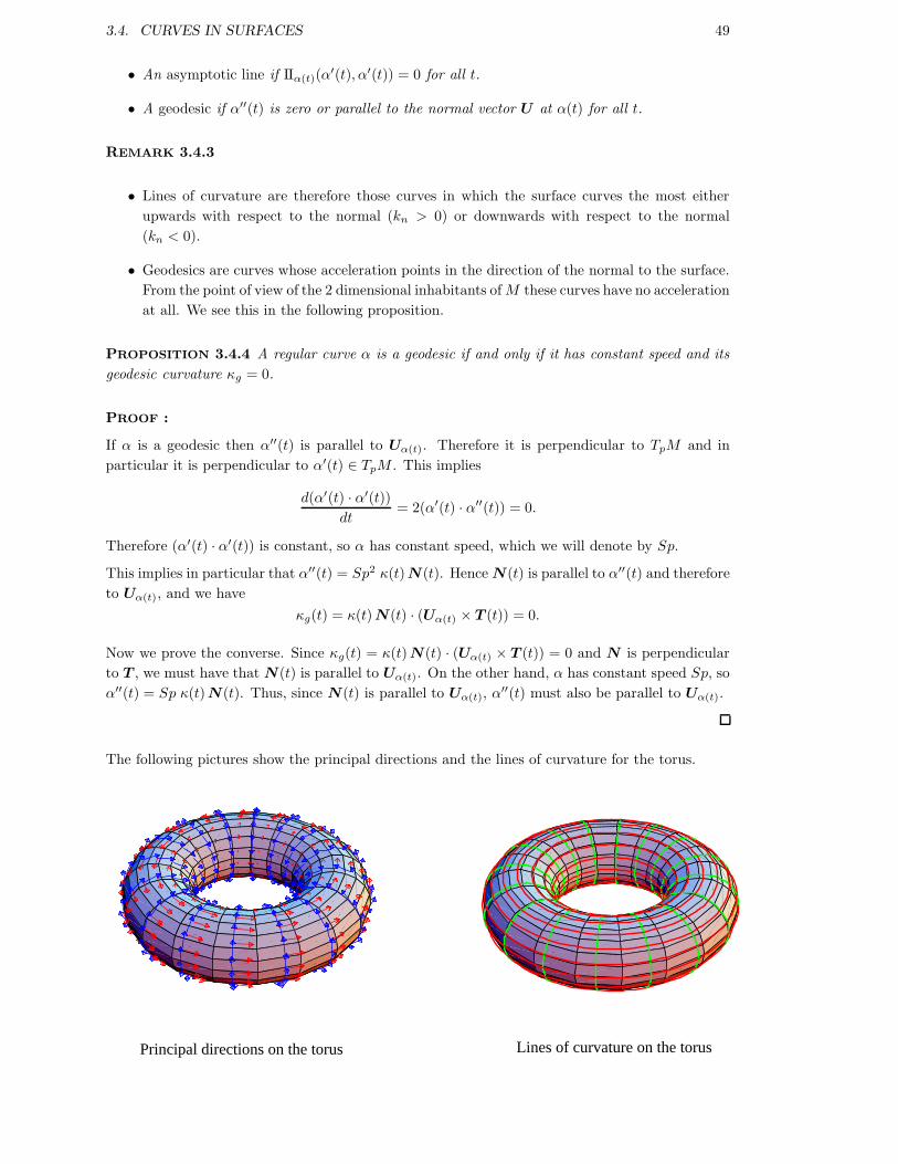
3.4. CURVES IN SURFACES 49
• An asymptotic line if IIα(t)(α′(t), α′(t)) = 0 for all t.
• A geodesic if α′′(t) is zero or parallel to the normal vector U at α(t) for all t.
REMARK 3.4.3
• Lines of curvature are therefore those curves in which the surface curves the most either
upwards with respect to the normal (kn > 0) or downwards with respect to the normal
(kn < 0).
• Geodesics are curves whose acceleration points in the direction of the normal to the surface.
From the point of view of the 2 dimensional inhabitants of M these curves have no acceleration
at all. We see this in the following proposition.
PROPOSITION 3.4.4 A regular curve α is a geodesic if and only if it has constant speed and its
geodesic curvature κg = 0.
PROOF :
If α is a geodesic then α′′(t) is parallel to Uα(t). Therefore it is perpendicular to TpM and in
particular it is perpendicular to α′(t) ∈ TpM . This implies
d(α′(t) · α′(t))
dt= 2(α′(t) · α′′(t)) = 0.
Therefore (α′(t) · α′(t)) is constant, so α has constant speed, which we will denote by Sp.
This implies in particular that α′′(t) = Sp2 κ(t) N(t). Hence N(t) is parallel to α′′(t) and therefore
to Uα(t), and we have
κg(t) = κ(t) N(t) · (Uα(t) × T (t)) = 0.
Now we prove the converse. Since κg(t) = κ(t) N(t) · (Uα(t) × T (t)) = 0 and N is perpendicular
to T , we must have that N(t) is parallel to Uα(t). On the other hand, α has constant speed Sp, so
α′′(t) = Sp κ(t) N(t). Thus, since N(t) is parallel to Uα(t), α′′(t) must also be parallel to Uα(t).
The following pictures show the principal directions and the lines of curvature for the torus.
Principal directions on the torus Lines of curvature on the torus
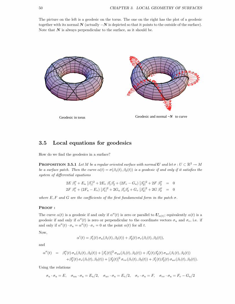
50 CHAPTER 3. LOCAL GEOMETRY OF SURFACES
The picture on the left is a geodesic on the torus. The one on the right has the plot of a geodesic
together with its normal N (actually −N is depicted so that it points to the outside of the surface).
Note that N is always perpendicular to the surface, as it should be.
Geodesic in torus −NGeodesic and normal to curve
3.5 Local equations for geodesics
How do we find the geodesics in a surface?
PROPOSITION 3.5.1 Let M be a regular oriented surface with normal U and let σ : U ⊂ R2 → M
be a surface patch. Then the curve α(t) = σ(β1(t), β2(t)) is a geodesic if and only if it satisfies the
system of differential equations
2E β′′1 + Eu [β′
1]2 + 2Ev β′
1β′2 + (2Fv − Gu) [β′
2]2 + 2F β′′
2 = 0
2F β′′1 + (2Fu − Ev) [β′
1]2 + 2Gu β′
1β′2 + Gv [β′
2]2 + 2G β′′
2 = 0
where E, F and G are the coefficients of the first fundamental form in the patch σ.
PROOF :
The curve α(t) is a geodesic if and only if α′′(t) is zero or parallel to Uα(t); equivalently α(t) is a
geodesic if and only if α′′(t) is zero or perpendicular to the coordinate vectors σu and σv , i.e. if
and only if α′′(t) · σu = α′′(t) · σv = 0 at the point α(t) for all t.
Now,
α′(t) = β′1(t) σu(β1(t), β2(t)) + β′
2(t) σv(β1(t), β2(t)),
and
α′′(t) = β′′1 (t) σu(β1(t), β2(t)) + [β′
1(t)]2 σuu(β1(t), β2(t)) + β′
1(t)β′2(t) σuv(β1(t), β2(t))
+β′′2 (t) σv(β1(t), β2(t)) + [β′
2(t)]2 σvv(β1(t), β2(t)) + β′
1(t)β′2(t) σuv(β1(t), β2(t)).
Using the relations
σu · σu = E, σuu · σu = Eu/2, σuv · σu = Ev/2, σv · σu = F, σvv · σu = Fv − Gu/2
3.6. AN INTERPRETATION OF GAUSSIAN CURVATURE 51
σuu · σv = Fu − Ev/2, σvv · σv = Gv/2, σuv · σv = Gu/2, σv · σv = G
we find
2α′′(t) · σu(β1(t), β2(t)) = 2Eβ′′1 + Eu[β′
1]2 + 2Evβ′
1β′2 + (2Fv − Gu)[β′
2]2 + 2Fβ′′
2
and
2α′′(t) · σv(β1(t), β2(t)) = 2Fβ′′1 + (2Fu − Ev)[β′
1]2 + 2Guβ′
1β′2 + Gv [β′
2]2 + 2Gβ′′
2
Hence α = σ(β1(t), β2(t)) is a geodesic if and only if β1 and β2 satisfy the following system of
second order differential equations.
2E β′′1 + Eu [β′
1]2 + 2Ev β′
1β′2 + (2Fv − Gu) [β′
2]2 + 2F β′′
2 = 0
2F β′′1 + (2Fu − Ev) [β′
1]2 + 2Gu β′
1β′2 + Gv [β′
2]2 + 2G β′′
2 = 0
In general it is difficult to solve these equations. Note that, being a system of 2 second order
equations, we need 4 initial conditions, normally the value of the curve α at some point and its
velocity at that point.
Facts about geodesics: We list some important and interesting facts that we shall not prove.
• Given two different points in a surface there is always a geodesic passing through these points.
• Among all the geodesics through two given points, there is one that has shortest length. In
fact, this shortest geodesic gives the shortest path to get from one point to the other
while staying in the surface. In other words, it is for the 2D inhabitants of the surface what
a straight line is for us.
3.6 An interpretation of Gaussian curvature
Gaussian curvature turns out to be the main invariant of surfaces, in the sense that two surfaces
with the same first fundamental form will have the same Gaussian curvature (we will see this fact
later). But we have not quite given a geometric interpretation of curvature yet.
Note that, although the shape operator, the second fundamental form, the principal curvatures and
the mean curvature change sign when we change the orientation of the surface, Gaussian curvature
does not since the determinant of a 2 by 2 matrix is equal to the determinant of minus that matrix.
DEFINITION 3.6.1 Let M be a regular surface. A point p in M is called
• Elliptic if K(p) > 0.
• Hiperbolic if K(p) < 0.
• Parabolic if K(p) = 0 but one of the principal curvatures at p is not 0 (or equivalently Sp is
not 0).
• Planar if the principal curvatures at p are both 0 (or equivalently Sp is 0).
• Umbillic if the principal curvatures at p are equal.
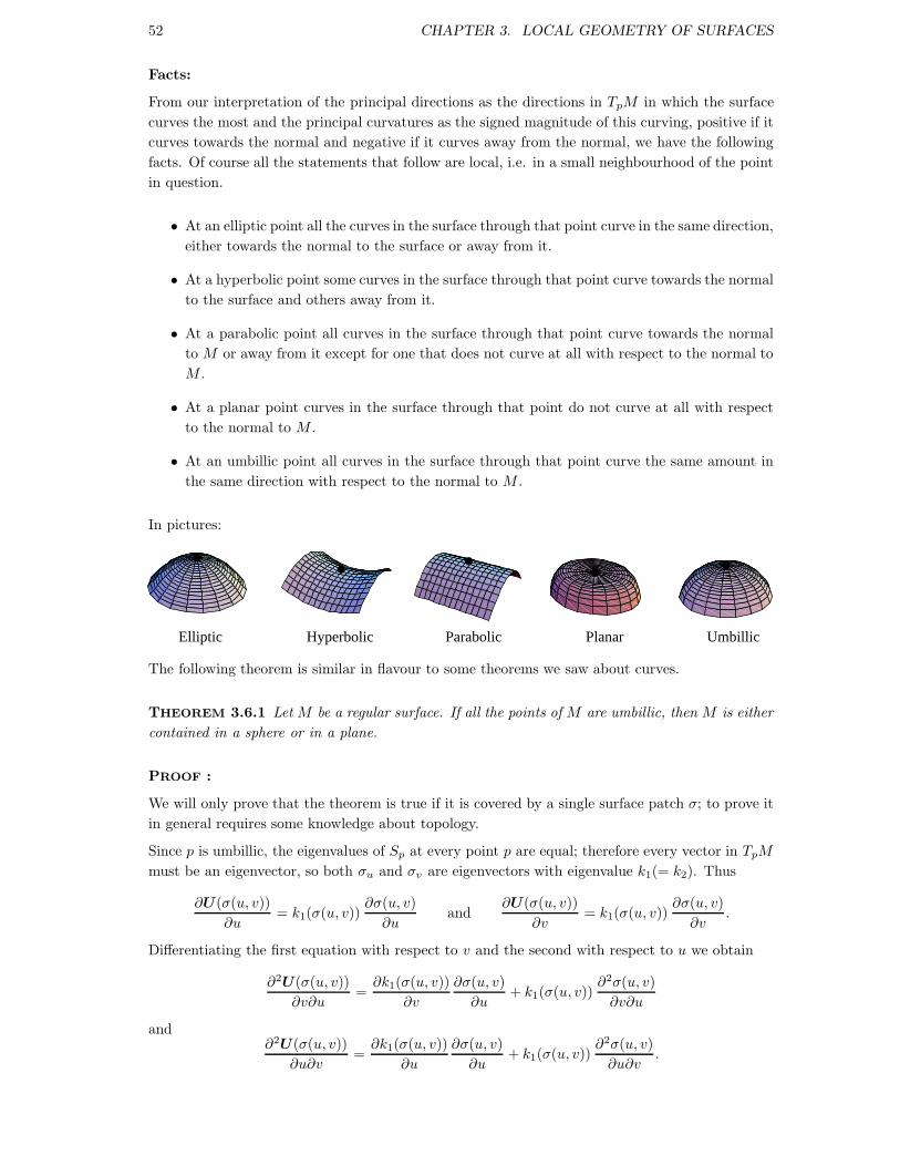
52 CHAPTER 3. LOCAL GEOMETRY OF SURFACES
Facts:
From our interpretation of the principal directions as the directions in TpM in which the surface
curves the most and the principal curvatures as the signed magnitude of this curving, positive if it
curves towards the normal and negative if it curves away from the normal, we have the following
facts. Of course all the statements that follow are local, i.e. in a small neighbourhood of the point
in question.
• At an elliptic point all the curves in the surface through that point curve in the same direction,
either towards the normal to the surface or away from it.
• At a hyperbolic point some curves in the surface through that point curve towards the normal
to the surface and others away from it.
• At a parabolic point all curves in the surface through that point curve towards the normal
to M or away from it except for one that does not curve at all with respect to the normal to
M .
• At a planar point curves in the surface through that point do not curve at all with respect
to the normal to M .
• At an umbillic point all curves in the surface through that point curve the same amount in
the same direction with respect to the normal to M .
In pictures:
Elliptic Hyperbolic Parabolic Planar Umbillic
The following theorem is similar in flavour to some theorems we saw about curves.
THEOREM 3.6.1 Let M be a regular surface. If all the points of M are umbillic, then M is either
contained in a sphere or in a plane.
PROOF :
We will only prove that the theorem is true if it is covered by a single surface patch σ; to prove it
in general requires some knowledge about topology.
Since p is umbillic, the eigenvalues of Sp at every point p are equal; therefore every vector in TpM
must be an eigenvector, so both σu and σv are eigenvectors with eigenvalue k1(= k2). Thus
∂U(σ(u, v))
∂u= k1(σ(u, v))
∂σ(u, v)
∂uand
∂U(σ(u, v))
∂v= k1(σ(u, v))
∂σ(u, v)
∂v.
Differentiating the first equation with respect to v and the second with respect to u we obtain
∂2U(σ(u, v))
∂v∂u=
∂k1(σ(u, v))
∂v
∂σ(u, v)
∂u+ k1(σ(u, v))
∂2σ(u, v)
∂v∂u
and∂2U(σ(u, v))
∂u∂v=
∂k1(σ(u, v))
∂u
∂σ(u, v)
∂u+ k1(σ(u, v))
∂2σ(u, v)
∂u∂v.
3.7. EXAMPLE: SURFACES OF REVOLUTION 53
Since second derivatives commute we have
∂k1(σ(u, v))
∂vσu =
∂k1(σ(u, v))
∂uσv ,
and since σu and σv are linearly independent, we must have
∂k1(σ(u, v))
∂v=
∂k1(σ(u, v))
∂u= 0,
proving that k1 is constant.
Now we integrate the equations
∂U(σ(u, v))
∂u= k1
∂σ(u, v)
∂uand
∂U(σ(u, v))
∂v= k1
∂σ(u, v)
∂v,
obtaining
U(σ(u, v)) = k1σ(u, v) + ~p0
for some constant vector ~p0.
If k1 = 0 then U is constant. Let σ(u0, v0) be a point in M , and consider the function
g(u, v) = (σ(u, v) − σ(u0, v0)) · U .
Then, since U is constant, gu(u, v) = σu · U = 0 and gv(u, v) = σv · U = 0, which implies that
f(u, v) is constant. Since f(u0, v0) = 0 we must have
f(u, v) = (σ(u, v) − σ(u0, v0)) · U = 0 for all u, v,
which expresses the fact that the image of σ lies in the plane through σ(u0, v0) perpendicular to
the constant vector U .
If k1 6= 0, then
σ(u, v) +~p0
k1=
U(σ(u, v))
k1,
and therefore∥
∥
∥
∥
σ(u, v) −(
−~p0
k1
)∥
∥
∥
∥
=1
|k1|which means that the image of σ lies in a sphere centred at −~p0/k1 with radius 1/k1.
3.7 Example: Surfaces of revolution
A surface of revolution is the surface obtained when a curve is rotated around an axes. Suppose
that the rotation axes is the z-axes and let the curve be (0, r(s), h(s)) for s ∈ (a, b); without loss
of generality we assume that the curve is parametrised by arc length (so (r′)2 + (h′)2 = 1). For
the surface to be regular we need to assume that r > 0.
A patch of the surface is
σ(u, v) = (r(v) cos u, r(v) sin u, h(v)), 0 < u < 2π, a < v < b.
σ covers all the surface except for a curve, but changing the domain of σ all the surface gets
covered. So we will do all calculations using σ.
We have
σu = (−r(v) sin u, r(v) cos, 0) σv = (r′(v) cos u, r′(v) sin u, h′(v)).

54 CHAPTER 3. LOCAL GEOMETRY OF SURFACES
Therefore
[I]σ =
(
[r(v)]2 00 1
)
, so E = [r(v)]2, F = 0, G = 1.
We have σu × σv = r(v) (h′(v) cos u, h′(v) sin u,−r′(v)); this has norm r(v), so we will take
U = (h′(v) cos u, h′(v) sin u,−r′(v))
as the unit normal. The matrix expression of the second fundamental form (recall that the coeffi-
cients are given by e = σuu · U , f = σuu · U , g = σvv · U) is
[II]σ =
(
−r(v)h′(v) 00 r′′(v)h′(v) − r′(v)h′′(v)
)
.
Since (r′)2 + (h′)2 = 1, r′r′′ = −h′h′′, so r′′h′ − r′h′′ = r′′h′ + (r′)2r′′/h′ = r′′/h′. Thus,
[II]σ =
(
−r(v)h′(v) 00 r′′(v)/h′(v)
)
.
Therefore the matrix expression for the shape operator in the patch σ is
[S]σ = [I]−1σ [II]σ =
−h′(v)
r(v)0
0 r′′(v)/h′(v)
.
We immediately obtain that
• The principal directions are σu and σv with corresponding principal curvatures −h′(v)/r(v)
and r′′(v)h′(v) − r′(v)h′′(v).
• Therefore the parallels σ(t, v0) and the meridians σ(u0, t) are lines of curvature.
• The gaussian curvature is K(σ(u, v)) = − r′′(v)
r(v).
This means that the sign of K depends only on the concavity or
convexity of r(v).
K > 0
K < 0
K < 0
Now we find the geodesics. We have
E = [r(v)]2, F = 0, G = 1, Eu = 0, Ev = 2r(v)r′(v), Fu = Fv = Gu = Gv = 0.
We use Proposition 3.5.1. we have that α(t) = σ(β1(t), β2(t)) is a geodesic if and only if (to
simplify the notation, let us write β1(t) = u and β2(t) = v; we will not write the argument ‘t’ but
we should not forget that u and v are functions of t, and that all the dashes are derivatives with
respect to t; the subscripts v mean derivatives with respect to v.)
2[r(v)]2 u′′ + 4 r(v) rv(v) u′ v′ = 0
−r(v) rv(v) [u′]2 + 2v′′ = 0
The first equation can be written as
( [r(v)]2 u′ )′ = 0,
and therefore
[r(v)]2 u′ = c
for some constant c. Now we know that a geodesic has constant speed Sp, so
α′(t) · α′(t) = (u′σu + v′σv) · (u′σu + v′σv) = E(u′)2 + 2Fu′v′ + G(v′)2 = Sp2.

3.7. EXAMPLE: SURFACES OF REVOLUTION 55
Therefore,
[r(v)]2(u′)2 + (v′)2 = Sp2.
Now substitute [r(v)]2 u′ = c in the previous equation to obtain
c2 + [r(v)]2(v′)2 = Sp2[r(v)]2.
This equation can be integrated to obtain v and then the equation [r(v)]2 u′ = c can be integrated
to obtain u.
The main interesting point in this discussion is the following. It is clear from the parametrization
that σu is tangent to a parallel of the surface (i.e. σu is parallel to the xy-plane). Now observe
that
α′(t) · σu = (u′σu + v′σv) · σu = Eu′ = [r(v)]2 u′ = c.
Since α′(t) · σu = ‖α′(t)‖ ‖σu‖ cos θ = Sp r(v) cos θ, where θ is the angle between α′(t) and a
parallel, we obtain Sp r(v) cos θ = c. Since Sp is constant, we can rewrite this as (Clairaut’s
relation):
r(v) cos θ = constant.
In other words, the cosine of the angle that a geodesic makes with the horizontal is
inversely proportional to the distance to the axis of rotation.
There are some geodesics that are easy to find. The meridians σ(u0, t) are geodesics since in
this case we have u′ = 0 and v′ = 1, so the system of equations above is clearly satisfied.
Are the parallels α(t) = σ(t, v0) geodesics? Not in general. Let us see the conditions for a parallel
to be a geodesic. Plugging in u = t, v = v0 in the equations above we see that the first equation
is satisfied (since both u′′ and v′ are 0). Since u′ = 1 and v′′ = 0, the second equation becomes
−r(v0) r′(v0) = 0.
Since r is never 0, this implies that a parallel σ(t, v0) is a geodesic if and only if r′(v0) = 0; in
other words, the only parallels of a surface of revolution that are geodesics are the ‘waists’ and the
‘hips’.
It is immediate to check that any meridian parametrised with constant speed is also a geodesic as
the equations are clearly satisfied (plug in, for example, u = u0 and v = t).
In pictures:
Geodesics

56 CHAPTER 3. LOCAL GEOMETRY OF SURFACES
3.8 Gauss Theorema Egregium
In this section we look at Gauss’ remarkable theorem that says that the Gaussian curvature only
depends on the first fundamental form. This is extraordinary: it means that by means of mea-
surements only on the surface one should be able to figure out how curved the surface is. In other
words, the 2 dimensional inhabitants of a surface are able to find out, for example, whether they
are standing in an elliptic, hyperbolic o parabolic point.
Recall that for curves we differentiated the tangent in order to obtain information about the shape
of the curve. So far for surfaces we have differentiated the normal. One reason for this is that
there is not one tangent vector but a whole plane of them.
Let us try to do a similar analysis. Take a coordinate patch σ in a regular oriented surface M .
Then {σu, σv , U} form a basis of R3 at each point σ(u, v) of the surface. This is kind of the Frenet
frame that we had for surfaces except for the very important fact that it is not an orthonormal
basis.
Let us differentiate these three vectors in the direction of σu and σv as we did in the case of curves
for the Frenet frame. First, the normal is easy:
DσuU = −s11σu − s21σv , Dσv
U = −s12σu − s22σv ,
where the sij are the coefficients of the matrix representation of the shape operator in the basis
σu and σv , i.e.
[S]σ =
(
s11 s12
s21 s22
)
.
The other derivatives can be written as
Dσuσu = Γ1
11σu + Γ211σv + L1U
Dσuσv = Γ1
12σu + Γ212σv + L2U
Dσvσv = Γ1
22σu + Γ222σv + L3U
Where Γ111, Γ
211, Γ
112, Γ
212, Γ
122, Γ
222 are some coefficients, called the Christoffel symbols. We do not
calculate Dσvσu because it is equal to Dσu
σv .
Note that L1 = (Dσuσu) ·U = −σu ·Dσu
U = II(σu, σu) = e in the traditional notation. Similarly,
L2 = f and L3 = g. So our complete set of equations is
Dσuσu = Γ1
11σu + Γ211σv + eU
Dσuσv = Γ1
12σu + Γ212σv + fU
Dσvσv = Γ1
22σu + Γ222σv + gU
DσuU = −s11σu − s21σv
DσvU = −s12σu − s22σv
To find the Christoffel symbols, dot-multiply each equation by σu and σv to obtain
Γ111E + Γ2
11F = σuu · σu = Eu/2
Γ111F + Γ2
11G = σuu · σv = Fu − Ev/2
Γ112E + Γ2
12F = σuv · σu = Ev/2
Γ112F + Γ2
12G = σuv · σv = Gu/2
Γ122E + Γ2
22F = σvv · σu = Fv − Gu/2
Γ122F + Γ2
22G = σvv · σv = Gv/2
3.8. GAUSS THEOREMA EGREGIUM 57
where we have used the relations
σu · σu = E, σuu · σu = Eu/2, σuv · σu = Ev/2, σv · σu = F, σvv · σu = Fv − Gu/2
σuu · σv = Fu − Ev/2, σvv · σv = Gv/2, σuv · σv = Gu/2, σv · σv = G
The point is that we have six equations for six variables Γ111, Γ
211, Γ
112, Γ
212, Γ
122, Γ
222. Therefore the
Christoffel symbols can be obtained in terms of the coefficients E, F, G of the first
fundamental form. Now it turns out that the curvature can be found in terms of these symbols,
as we will now see.
We complicate things further: note that since multiple derivatives commute we have relations of
the sort
DσvDσu
σu = σvuu = σuvu = DσuDσv
σu
DσvDσv
σu = σvvu = σvuv = DσvDσu
σv
DσvDσu
U = DσuDσv
U
and many more (although it turns out that the rest of the relations do not add any more information—
these are it!). These equations can be rewritten as
0 = DσvDσu
σu − DσuDσv
σu
0 = DσvDσv
σu − DσvDσu
σv
0 = DσvDσu
U − DσuDσv
U .
If now we plug in the original equations into these ones (formidable task!) we will get many
relations. It turns out that all the possible relations get summarised into three equations. The
first is the following, called the Gauss equation. The subscripts u or v mean, as usual, derivatives
with respect to u or v:
(Γ212)u − (Γ2
11)v + Γ112Γ
211 + Γ2
12Γ212 − Γ2
11Γ222 − Γ1
11Γ212 = −E
eg − f2
EG − F 2= −E K.
This implies in particular that K can be obtained solely from the coefficients of the first
fundamental form and no further information. This is
THEOREM 3.8.1 (Gauss Theorema Egregium) The Gaussian curvature K of a surface depends
only on the first fundamental form. Therefore if we change the surface while preserving lengths
and angles in the surface the curvature does not change.
The two other relations are the Codazzi-Mainardi equations:
ev − fu = eΓ112 + f(Γ2
12 − Γ111 − gΓ2
11)
fv − gu = eΓ122 + f(Γ2
22 − Γ112 − gΓ2
12)
Remember that for curves we had a theorem that said that given functions κ > 0 and τ there
was a unique curve with curvature κ and torsion τ up to rigid motion. For surfaces we have an
equivalent theorem:
THEOREM 3.8.2 (Bonnet) Given functions E, F, G and e, f, g defined in an open set in R2 with
E > 0, G > 0 and EG−F 2 > 0 that satisfy the Gauss formula and the Codazzi-Mainardi equations
there is a parametrised surface σ(V ) ⊂ R3 whose coefficients of the first and second fundamental
form are the given E, F, G and e, f, g; furthermore, any two surfaces with these characteristics
differ only by a rigid motion.