diagnosis and fault detection in electrical machines and

Department of Electrical, Electronic, and Information Engineering “Guglielmo Marconi”

Ph.D thesis of:

Yasser Gritli

Ph.D. in Electrical Engineering XXVI Cycle

Power Electronics, Electrical Machines and Drives (ING-IND/32)

Diagnosis and Fault Detection in Electrical Machines and Drives

based on Advanced Signal Processing Techniques

Tutor :

Prof. Fiorenzo Filippetti

Final dissertation on March 2014

Ph.D. Coordinator:

Prof. Domenico Casadei

i

CONTENT

Content ..................................................................................................................................................... i Liste of figures ...................................................................................................................................... iv

List of tables ........................................................................................................................................... x

Nomenclature ........................................................................................................................................ xi Preface .................................................................................................................................................... 1 Chapter 1 : State of art in diagnostic for electrical machines ............................................ 4 1.1 Introduction .............................................................................................................................. 5 1.2 Stator related-faults .................................................................................................................. 6

1.2.1 Stator faults physics .......................................................................................................... 6 1.2.2 Stator fault components propagation ........................................................................... 7

1.3 Rotor related-faults .................................................................................................................. 9 1.3.1 Rotor faults physics .......................................................................................................... 9 1.3.2 Rotor fault components propagation ........................................................................ 11

1.4 Signal processing techniques for electrical machines diagnosis ................................... 12 1.5 Conclusion ............................................................................................................................. 15

References ........................................................................................................................................... 16 Chapter 2 : Developed approach for diagnosing electrical machines .......................... 23 2.1 Introduction ........................................................................................................................... 24 2.2 Signals and processing tools for faults characterization ................................................ 24

2.2.1 Signals selection for processing................................................................................... 24 2.2.2 Signal Processing tools ................................................................................................. 25

2.2.2.1 Fourier Transform ............................................................................................. 25 2.2.2.2 Short Time Fourier Transform ....................................................................... 26 2.2.2.3 Wavelet Transform ............................................................................................ 27

2.3 Problematic and developed Diagnosis approach............................................................ 30 2.4 Proposed diagnostic approach ........................................................................................... 34 2.5 Conclusion ............................................................................................................................. 39 References ............................................................................................................................................ 40 Chapter 3 : Analysis of stator and rotor faults in wound rotor induction machines44 3.1 Introduction ........................................................................................................................... 45 3.2 System description ................................................................................................................ 45

3.2.1 WRIM Control system ................................................................................................. 45 3.2.2 Experimental system ..................................................................................................... 49

3.3 Results ..................................................................................................................................... 51

ii

3.3.1 Fault detection under speed-varying condition........................................................ 51 3.3.1.1 Stator dissymmetry detection .......................................................................... 52 3.3.1.2 Rotor dissymmetry detection .......................................................................... 55

3.3.2 Fault detection under fault-varying conditions ........................................................ 56 3.3.2.1 Stator progressive dissymmetry detection ..................................................... 58 3.3.2.2 Rotor progressive dissymmetry detection ..................................................... 60

3.4 Fault quantification ............................................................................................................... 60 3.5 Conclusion ............................................................................................................................. 65 References ............................................................................................................................................ 66 Chapter 4 : Analysis of rotor faults squirrel cage induction machines........................ 68 4.1 Introduction ........................................................................................................................... 69 4.2 Analysis of rotor fault in single cage induction machine ............................................... 69

4.2.1 System description ......................................................................................................... 69 4.2.2 Results .............................................................................................................................. 70

4.2.2.1 Fault detection under speed-varying conditions .......................................... 70 4.2.2.2 Fault quantification ............................................................................................ 74

4.3 Analysis of rotor fault in double cage induction machine ............................................ 76 4.3.1 Motor Current Signature Analysis .............................................................................. 78

4.3.1.1 System description ............................................................................................. 78 4.3.1.2 Results .................................................................................................................. 78

4.3.2 Motor Vibration Signature Analysis ........................................................................... 83 4.3.2.1 System description ............................................................................................. 84 4.3.2.2 Results .................................................................................................................. 85

4.4 Conclusion ............................................................................................................................. 90

References ........................................................................................................................................... 91 Chapter 5 : Fault diagnosis extension for multiphase electrical machines................. 94 5.1 Introduction ........................................................................................................................... 95 5.2 Characterization of Rotor Demagnetization in Five-Phase Surface–Mounted Permanent Magnet Generator .......................................................................................................... 95

5.2.1 System description ......................................................................................................... 95 5.2.1.1 Results ................................................................................................................ 102 5.2.1.2 Fault quantification .......................................................................................... 104

5.3 Characterization of stator fault in seven-phase induction machine .......................... 104 5.3.1 System description ....................................................................................................... 105 5.3.2 Results ............................................................................................................................ 106

5.4 Conclusion ........................................................................................................................... 109

References ......................................................................................................................................... 110 Conclusions ...................................................................................................................................... 112

Appendix. 1: WRIM Model .......................................................................................................... 114

Appendix. 2: Multiple Space Vector representation ............................................................... 117

iv

LISTE OF FIGURES

Fig. 1.1 Distribution of failures by motor component ........................................................ 5

Fig. 1.2 Pareto of problems resulting in reduced motor efficiency (increased

electrical losses) in electrical distribution systems. ................................................ 7

Fig. 1.3 Frequency domain propagation of a stator fault. ................................................... 9

Fig. 1. 4 Rotor fault repartition in squirrel cage induction motors. .................................. 10

Fig. 1. 5 Example of 3.3 kV, 800kW double cage induction motor failure due to

outer cage damage: (a) outer bar damage, (b) stator end-winding insulation

failure due to broken copper fragments from outer bar ....................................... 11

Fig. 1.6 Frequency domain propagation of a rotor fault. .................................................. 12

Fig. 1.7 Block topology of signal-based diagnostic procedure ....................................... 13

Fig. 2. 1 Constant resolution in time-frequency plane using Short-time Fourier

Transform .............................................................................................................. 27

Fig. 2. 2 Multiresolution in time-frequency plane using Wavelet Transform ................. 28

Fig. 2. 3 Wavelet Transform using a filter banks ............................................................. 29

Fig. 2. 4 Percentage of wavelet applications for different power system areas ............... 30

Fig. 2. 4 Experimental results: Rotor modulating signal spectrum for large speed

transient under healthy (red line) and stationary stator High-resistance

connection (blue line). ........................................................................................... 32

Fig. 2. 5 Experimental results: Rotor modulating signal spectrum for intermittent

stator High-resistance connection ......................................................................... 32

Fig. 2. 7 High-level wavelet signals resulting from the DWT of the startup current

for: (a) healthy machine and (b) machine with two broken bars. ........................ 33

Fig. 2. 8 Time-frequency propagation of a stator fault. The minus sign (–) identifies

current inverse sequence components .................................................................. 35

Fig. 2. 9 Time-frequency propagation of a rotor fault. The minus sign (–) identifies

current inverse sequence components .................................................................. 35

Fig. 2. 10 The DWT filtering process for decomposition of signal into

predetermined frequency bands ............................................................................ 37

v

Fig. 2. 11 Principle of time interval calculation as a function of the Time Interval

Number (TIN) ........................................................................................................ 38

Fig. 3. 1 Block-scheme representation of the complete WRIM control system ............. 48

Fig. 3. 2 Experimental set-up. a) Power converter cabinet. b) WRIM and prime

mover. c) Schematic diagram of the test bench and position of the current

and voltage sensors. ............................................................................................... 50

Fig. 3. 3 Discrete WT of krsslI and krs

slV in healthy condition (Radd=0) under speed

transient.................................................................................................................. 53


slV in faulty condition (Radd=Rs) under speed

transient.................................................................................................................. 54



transient (experimental results) ............................................................................. 54


slV in faulty condition (Radd=Rs) under speed


Fig. 3. 7 DWT of the signals krrslI and krr


transient (simulation results) ................................................................................. 56


slV in faulty condition (Radd=Rr) under speed

transient (simulation results) ................................................................................. 57





slV in faulty condition (Radd=Rr) under speed


Fig. 3. 11 Discrete WT of krsslV under progressive stator unbalance condition

(simulation results) ................................................................................................ 59


(experimental results) ............................................................................................ 59

Fig. 3. 13 Discrete WT of krrslV under progressive rotor unbalance condition

(simulation results) ................................................................................................ 61


(experimental results) ............................................................................................ 61

vi

Fig. 3. 15 Values of the fault indicator mPa8 (as a function of the Time Interval

Number) resulting from the 8th wavelet decomposition under stator

unbalance for large speed variation (simulation results): a) ( )rsslI t - b) ( )rs

slV t ........ 62


Number) resulting from the 8th wavelet decomposition under stator

unbalance for large speed variation (experimental results): a) ( )rsslI t - b) ( )rs

slV t .... 63


Number) resulting from the 8th wavelet decomposition under rotor

unbalance for large speed variation (simulation results): a) ( )rrslI t - b) ( )rr

slV t ......... 63


Number) resulting from the 8th wavelet decomposition under rotor

unbalance for large speed variation (experimental results): a) ( )rrslI t - b) ( )rr

slV t ..... 64

Fig. 3. 19 Values of the fault indicator mPa8 resulting from the 8th wavelet

decomposition of ( )rsslV t and ( )rr

slV t under progressive winding fault: a) stator

-b) rotor .................................................................................................................. 64

Fig. 4. 1 Test bed photo (left). The faulty rotor with one drilled rotor bar (right) ........... 70

Fig. 4. 2 Instantaneous values of a-b) speed and c-d) stator phase currents under

healthy and one rotor broken bar respectively ..................................................... 71

Fig. 4. 3 DWT analysis of stator phase current under speed-varying condition, for

tracking the fault component (1-2s)f ; Healthy condition .................................... 72


tracking the fault component (1-2s)f ; One Broken Bar ....................................... 73


tracking the fault component (1+2s)f ; Healthy condition ................................... 73


tracking the fault component (1+2s)f ; One Broken Bar ..................................... 74

Fig. 4. 7 Cyclic values of the fault indicator mPa9, resulting from the 9th wavelet

decomposition level of the signals Isl under healthy and rotor bar broken (red

and blue) during the tracking of (1-2s)f component ............................................. 75

Fig. 4. 8 Cyclic values of the fault indicator mPa9, resulting from the 9th wavelet

decomposition level of the signals Isl under healthy and rotor bar broken (red

and blue) during the tracking of (1+2s)f component ........................................... 75

vii

Fig. 4. 9 Electrical equivalent circuit representation of a double squirrel cage

induction motor ..................................................................................................... 77

Fig. 4. 10 Experimental measurements of broken bar component, frffc, with on-line

MCSA under rated load for 0-3/44 broken bars for (left) single cage deep

bar Al die cast rotor; (right) double cage fabricated brass-Cu separate end

ring rotor [7] .......................................................................................................... 77

Fig. 4. 11 Custom designed fabricated copper separate end ring double cage rotor

sample with brass outer cage and copper inner cage(a), and the

corresponding rotor lamination (b) ....................................................................... 78

Fig. 4. 12 DWT analysis of stator current under transient operating condition (10%-

90% rated load):a) speed profile, b) phase current, c) fl component, and d) fr

component under healthy conditions .................................................................... 80


90% rated load):a) speed profile, b) phase current, c) fl component, and d) fr

componentwith3 broken outer cage bars .............................................................. 81


50%-90% rated load): a) speed profile, b) phase current, c) fl component,

and d) fr component under healthy conditions ..................................................... 81


50%-90% rated load):a) speed profile, b) phase current, c) fl component, and

d) fr component with3 broken outer cage bars ..................................................... 82

Fig. 4. 16 Values of the fault indicators: normalized Find (Black line)resulting

from the 6th wavelet decomposition level of the stator current under healthy

and faulty (3 broken outer cage bars) conditions with speed-varying

conditions. Left side component (Blue line), and right side component (Red

line) 83

Fig. 4. 17 Photos of the healthy and drilled broken bar (left), and details of the

test-bed (right) ....................................................................................................... 84

Fig. 4. 18 Instantaneous values of speed (a), and axial vibration signal (b)

under healthy conditions ....................................................................................... 85

Fig. 4. 19 Instantaneous values of speed (a), and axial vibration signal (b)

under broken bar .................................................................................................... 85

Fig. 4. 20 Instantaneous values of axial vibration signal (a), and its

corresponding Wavelet analysis (b) under healthy condition .............................. 87

viii


corresponding Wavelet analysis (b) under rotor broken bar. ............................... 87


corresponding Wavelet analysis (b) under healthy condition .............................. 88


corresponding Wavelet analysis (b) under rotor broken bar. ............................... 88

Fig. 4. 24 Cyclic values of the mPa6 fault indicator calculation issued from

the approximation signal a6, under healthy (Red) and rotor broken bar

(Blue) conditions. .................................................................................................. 89

Fig. 4. 25 Cyclic values of the mPa7 fault indicator calculation issued from

the approximation signal a7, under healthy (Red) and rotor broken bar

(Blue) conditions. .................................................................................................. 90

Fig. 5. 1 Schematic draw of a pair of surface-mounted permanent magnets in

healthy and fault conditions .................................................................................. 97

Fig. 5. 2 Harmonic amplitude variation in the flux density distribution as a function

of the magnet pole arc reduction in electrical radians..................................... 98

Fig. 5. 3 Cross-section of the five-phase PMSG, with a superimposed flux plot

obtained by FEA, in healthy no-load conditions. ............................................... 101

Fig. 5. 4 Instantaneous values of the electrical speed (a), and the corresponding

back-emfs under faulty conditions ...................................................................... 102

Fig. 5. 5 Instantaneous values of the electrical speed (a), and the third

approximation signal (a3) issued from Wavelet analysis of the α3-β3

components of the back-emf space vector under healthy conditions. ............... 103

Fig. 5. 6 Instantaneous values of the electrical speed (a), and the third

approximation signal (a3) issued from Wavelet analysis of the α3-β3

components of the back-emf space vector under local rotor magnet

demagnetization conditions................................................................................. 103

Fig. 5. 7 Values of the fault indicator mPa3 (eS3), corresponding to the 7th inverse

harmonic component, resulting from the approximation signal a3 under

large speed transient, for healthy and local rotor demagnetization (15°)

conditions. ........................................................................................................................... 104

Fig. 5. 8 Experimental set-up. a) Schematic diagram of the test bench and position

of the current and voltage sensors. b) Seven phase induction machine. c)

Seven phase inverter ......................................................................................................... 106

ix

Fig. 5. 9 - Experimental result. Behavior of the drive in healthy condition. a)

Behavior of 3Si . b) Spectrum of 3Si . c) Trajectory of the components of 3Si at

25 Hz ................................................................................................................. 107

Fig. 5. 10 Experimental result. Behavior of the drive in healthy condition. a)

Behavior of 5Si . b) Spectrum of 5Si . c) Trajectory of the components of 5Si at

25 Hz ................................................................................................................. 107

Fig. 5. 11 Experimental result. Behavior of the drive when an additional resistance

is in series with phase 1. a) Behavior of 3Si . b) Spectrum of 3Si . c) Trajectory

of the components of 3Si at 25 Hz. ................................................................... 108



of the components of 5Si at 25 Hz. ................................................................... 108



of the components of 3Si at 25 Hz .................................................................... 108



of the components of 5Si at 25 Hz .................................................................... 109

x

LIST OF TABLES

Table. 2. 1 Fault harmonics Classification in term of Adopted input signals for

processing .............................................................................................................. 24

Table. 2. 2 Fault harmonics Frequency Bandwidth Repartition....................................... 36

Table. 3. 1 WRIM parameters .......................................................................................... 50

Table. 3. 2 Back-to-Back Converter Parameters ............................................................. 51

Table. 3. 3 Sensors ............................................................................................................ 51

Table. 4. 1 Single Cage Induction Motor parameters ....................................................... 70

Table. 4. 2 Frequency bands of approximation and detail signals .................................. 79

Table. 4. 3 Data of the double rotor cage motor .............................................................. 84

Table. 4. 4 Frequency bands at each level of decomposition .......................................... 86

Table. 5. 1 Five-Phase PMSG Parameters (FEA) ............................................................ 97

Table. 5. 2 Frequency band of each level ...................................................................... 103

Table. 5. 3 Parameters of the Seven-Phase Machine ..................................................... 105

xi

NOMENCLATURE

f Stator frequency

s Slip

ωr Rotor speed

θr Rotor position angle

θ Stator-flux phase angle

Rs Stator resistance

Rr Rotor resistance

Radd Additional resistance used during the tests

vds,vqs d−q components of the stator voltage vector in the synchronous reference

frame

ids,iqs d−q components of the stator current vector in the synchronous reference

frame

fsam Sampling frequency

flow,fup Lower and upper limits of the instantaneous fault frequency evolution

fkss,fkrs Frequencies of the kth stator and rotor harmonic components due to a stator

fault

fksr,fkrr Frequencies of the kth stator and rotor harmonic components due to a rotor

fault

Lm Mutual inductance between stator and rotor windings

Ls,Lr Stator and rotor self-inductances

idms,iqms d−q components of the magnetizing current in the synchronous reference

frame

ias,ibs,ics Stator phase currents

iar,ibr,icr Rotor phase currents

vas,vbs,vcs Stator phase voltage

vdr,vqr d−q components of the rotor modulating signals in the synchronous reference

frame

fsl Sliding frequency

mPaj Mean power value of approximation signal.

1

PREFACE

Condition monitoring leading to fault diagnosis and prediction of electrical machines

and drives has attracted researchers in the past few years because of its considerable

influence on the operational continuation of many industrial processes. Reducing

maintenance costs and preventing unscheduled downtimes, which result in lost

production and financial income, are the priorities of electrical drive manufacturers and

operators. In fact, correct diagnosis and early detection of incipient faults result in fast

unscheduled maintenance and short downtime for the process under consideration. They

also avoid harmful, sometimes devastating, consequences and reduce financial loss. An

ideal diagnostic procedure should take the minimum measurements necessary from a

machine and by analysis extract a diagnosis, so that its condition can be inferred to give

a clear indication of incipient failure modes in a minimum time. During the last years

there has been a considerable amount of research into the creation of new condition

monitoring techniques for induction motors and drives, overcoming the drawbacks of

traditional methods. More specifically, there has been a transition from techniques

suitable for machines in steady state conditions to machines operating in time-varying

conditions.

In the current thesis, a new diagnosis technique for electrical machines operating in

time-varying conditions is presented, where the validity under speed-varying condition

or fault-varying condition is validated.

The presented work was elaborated in five chapters organized as follows:

In the first chapter, the considered faults (stator, rotor electrical/mechanical faults) are

introduced, and a literature review of the corresponding diagnosis techniques are

presented and discussed.

The problematic of signal processing techniques used for electrical machine diagnosis

operating in time-varying conditions is firstly presented in the second chapter. Then, the

proposed approch is completely described and systematized in order to overcome limits

of existing techniques.

The proposed diagnosis technique is validated for the detection of electrical faults in

three-phase wound-rotor induction machines in the third chapter, where stator and rotor

electrical faults were investigated under time-varying conditions.

2

In the fourth chapter, the proposed diagnosis technique is validated for the detection of

rotor broken bars in single and double squirrel cage induction motors under time-

varying conditions.

Finally, the detection of rotor demagnetization, in five-phase surface-mounted

permanent magnet synchronous generators under time-varying conditions is

investigated in the fifth chapter, where stator fault detection and localization in seven-

phase induction machine is also investigated in time and frequency domains.

4

CHAPTER 1 : STATE OF ART IN

DIAGNOSTIC FOR ELECTRICAL

MACHINES

1.1 Introduction .............................................................................................................................. 5 1.2 Stator related-faults .................................................................................................................. 6

1.2.1 Stator faults physics .......................................................................................................... 6 1.2.2 Stator fault components propagation ........................................................................... 7

1.3 Rotor related-faults .................................................................................................................. 9 1.3.1 Rotor faults physics .......................................................................................................... 9 1.3.2 Rotor fault components propagation ........................................................................ 11

1.4 Signal processing techniques for electrical machines diagnosis ................................... 12 1.5 Conclusion ............................................................................................................................. 15

References ........................................................................................................................................... 16

5

1.1 Introduction

Condition monitoring of electrical machines has become a very important

technology in the field of electrical systems maintenance, mainly for its potential

functions of failure prediction, fault identification, and dynamic reliability estimation. In

this thesis, we make reference to induction machine, even if the discussed and proposed

diagnostic technique can be extended and applied also to other kind of machines. For

example to the permanent magnet machine as we can see in the following chapters.

Electrical machines are subject to different sorts of faults. Stator winding faults

including: turn to turn, coil to coil, open circuit, phase to phase, or coil to ground,

generally initiated by high-resistance connections. Rotor electrical faults which include

rotor open phase, rotor unbalance due to short circuits or high-resistance connections for

wound rotor machines, or rotor magnet demagnetization that can be caused by an over

current on the stator windings. Rotor mechanical faults such as broken bar(s) or cracked

end-ring for squirrel-cage machines, cracked rotor magnet, bearing damage,

static/dynamic eccentricity, and misalignment. The aforementioned failure modes can

potentially affect the good operating condition of any industrial system [1]-[4]. A recent

reliability study [4] has revealed the distribution of failures in induction motors as

illustrated in Fig. 1.1.

Fig. 1.1 Distribution of failures by motor component

During the last years there has been a considerable amount of research into the

creation of new condition monitoring techniques for induction motors and drives,

overcoming the drawbacks of traditional methods. In this context, different efficient and

non-invasive diagnosis techniques have been developed which investigate easily

measured electrical or mechanical quantities like for example current, external magnetic

Bearing69%

Stator Winding21%

Rotor bars7%

Shaft/Coupling3%

6

field, speed and vibrations, in order to detect the above listed failure modes at incipient

stage of degradation. [5]-[8]. The topic is becoming far more attractive and critical as the

population of electric machines has largely increased in recent years: the number of

operating machines is about 16.1 billion in 2011, with a growth of about 50% in the last

five years [9].

In this chapter, the considered faults (stator, rotor electrical/mechanical faults) are

introduced, and a literature review of the corresponding diagnosis techniques are

presented and discussed.

1.2 Stator related-faults

1.2.1 Stator faults physics

According to a recent reliability study, stator winding faults are of 21% ovrall

distribution of failures by motor component [4]. This category of faults can be observed

in different forms in electrical machines such as: turn to turn, coil to coil, open circuit,

phase to phase, or coil to ground. Obviously consequences on the performances

operating of the motor are different. In case of asymmetry in the stator windings such as

an open-phase failure or high-resistance connection, the machine can operate, but with

reduced torque. But in case of short-circuit of a few turns in a phase winding, the fault

evolve rapidly in time, and leads to catastrophic damages.

It is universally known, that an electrical or magnetic non rotational asymmetry of

induction machine or an asymmetry in the supply voltages can be detected through the

stator current negative sequence. The machine behavior is not the ideal one but no

drastic action must be taken in case of small asymmetries. A strong electric asymmetry,

as an open phase, causes a negative sequence of similar magnitude compared with the

positive one. This failure mode can be is therefore easily detected, and the protection

system is triggered.

Winding short circuit is well known as one of the most difficult faults to detect at

incipient stage. The standard protection might not work or the motor might keep on

running while the heating in the shorted turns would soon cause critical insulation

breakdown. If left undetected, turn faults will propagate, leading to phase to ground or

phase to phase faults.

Then it is important to note that this failure mode is generally initiated by high-

resistance connections caused by a combination of poor workmanship, thermal cycling

7

and vibration, or damage of the contact surfaces due to pitting, corrosion or

contamination.

The increase in the resistance due to poor contacts can cause overheating to reach

an unacceptable level, which can eventually leads to open-circuit failures due to the

melting of copper conductors. Eventually, excessive overheating in the contact points

can also deteriorate insulation and expose the copper conductor to serious damages such

as short-circuit failures between conductors or to the ground.

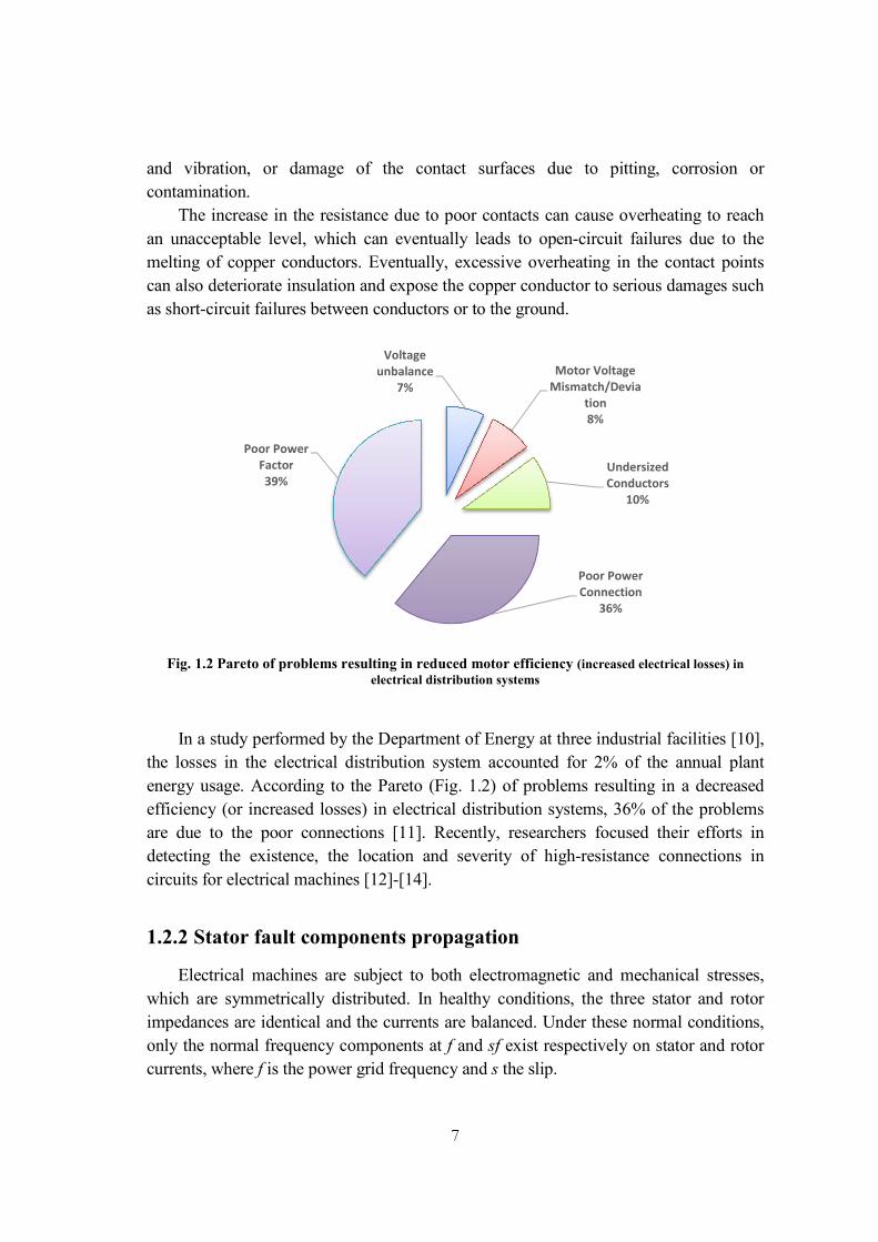
Fig. 1.2 Pareto of problems resulting in reduced motor efficiency (increased electrical losses) in electrical distribution systems

In a study performed by the Department of Energy at three industrial facilities [10],

the losses in the electrical distribution system accounted for 2% of the annual plant

energy usage. According to the Pareto (Fig. 1.2) of problems resulting in a decreased

efficiency (or increased losses) in electrical distribution systems, 36% of the problems

are due to the poor connections [11]. Recently, researchers focused their efforts in

detecting the existence, the location and severity of high-resistance connections in

circuits for electrical machines [12]-[14].

1.2.2 Stator fault components propagation

Electrical machines are subject to both electromagnetic and mechanical stresses,

which are symmetrically distributed. In healthy conditions, the three stator and rotor

impedances are identical and the currents are balanced. Under these normal conditions,

only the normal frequency components at f and sf exist respectively on stator and rotor

currents, where f is the power grid frequency and s the slip.

Voltage unbalance

7%

Motor Voltage Mismatch/Devia

tion8%

Undersized Conductors

10%

Poor Power Connection

36%

Poor Power Factor39%

8

If the stator is damaged, the stator symmetry of the machine is lost and a reverse

rotating magnetic field is produced. Let us assume that the stator and rotor voltages are

not altered by the fault and that the machine speed is free to vary. Then, a frequency

component appears in the stator current at frequency –f. This inverse sequence is

reflected on the rotor side and produces the frequency component (s-2)f, which induces

a pulsating torque and a speed oscillation at frequency 2f. This frequency generates both

a reaction current at frequency (s-2)f and a new component at frequency (s+2)f. The

latter produces new components in the stator currents at frequencies ±3f, and the process

starts again. In conclusion, it leads to a set of new components at frequencies expressed

by (1.1) and (1.2), in the stator and rotor currents respectively.

0,1,2,( 1 2 )kss kf k f (1. 1)

0,1,2,( 2 )krs kf s k f (1. 2)

Fig. 1.3 gives a graphical interpretation of the aforementioned propagation

mechanism of the fault harmonics. It is worth noting that this interpretation is just

qualitative and may help the reader to understand the effect of a fault, but does not

provide either a quantitative or an accurate description of all the phenomena involved

[15].

Generally, the main focus are on the detection of fault dominant frequency

components in stator signals at the frequency −sf and at the frequency (s−2)f in rotor

signals. Fig. 1.3 shows the stator fault propagation in frequency domain. This fault can

be monitored and detected in a variety of methods. In fact, the equivalent parameters of

the machine are changed, the currents are not balanced, and all the quantities linked to

the currents are affected by the faults. But in closed-loop operation the control system

ensures a safe operation even under an unbalance in stator windings. Therefore, the

typical rotor current fault frequency components is reduced by the compensating action

of the control system. However, under these conditions the fault-related frequencies are

reflected in the voltages that can be used for fault detection [15-16].

9

Frequency domain

sf

2f

±3f

Rotorfrequencies

Statorfrequencies

Mechanicalspeed

frequencies

± f

(s -2)f

(s+2)f

Fig. 1.3 Frequency domain propagation of a stator fault. The minus sign (–) identifies current inverse sequence components

1.3 Rotor related-faults

1.3.1 Rotor faults physics

Different faults can affect the rotor part of induction motors, which were

repartitioned in [17] and illustrated by Fig. 1.4. Squirrel cage machines can be classified

in two different types of cage rotors for induction motors: cast (up to 3000-kW rating)

and fabricated. Fabricated cages are used for higher ratings and special application

machines, where possible failure events occur on bars and end-ring segment. Cast rotors

are almost impossible to repair after bar breakage or cracks, although they are more

durable and rugged than fabricated cages. Typically, they are used in laboratory tests to

validate diagnostic procedures for practical reasons. Broken bar and cracked end ring

faults share only 7 % of induction machine faults, but the detection of these events is a

key item. In case of stator faults machine operation after the fault is limited to a short

time, but in case of rotor faults the machine operation after the fault is not restricted

apart from suitable caution during maintenance. On the other side the current in the rotor

bar adjacent to the faulty one increases remarkably, up to 50 % of nominal current,

while in the stator faulty winding the current variation is a few percent of the nominal

current. Another special and interesting case is for double-cage induction motors.

Doubly squirrel cage induction motors (DCIMs) are commonly used for applications in

which high starting torque and efficient steady state operation are required, such as

conveyors, pulverizers, or mills [18]. In these applications, DCIMs are subject to fatigue

10

failure of the outer (“starting”) cage, due to the cyclic thermal/mechanical stress caused

by frequent starts and long startup time [19]-[22].

Fig. 1. 4 Rotor fault repartition in squirrel cage induction motors.

Failure of outer cage bars tends to spread to neighboring bars as the currents of the

damaged bars are distributed into them. This could eventually result in startup failure

due to insufficient startup torque [23]. An example of a DCIM failure with outer cage

bar damage is shown in Fig. 1.5. This 800 kW, 3.3kV pulp stirrer motor recently failed

in a paper mill in Korea. The inner cage was in good condition. On the contrary, the

excessive thermal and thermo-mechanical stress due to outer cage damage resulted in

“melting” and “fracture” of the outer bars (the temperature exceeded 200°C) [22]. This

produced copper bar fragments that caused stator end winding insulation and core

damage, and led to irreversible motor failure.

For wound-rotor machines, the physics of rotor fault is similar to stator fault and it

results either in an increase of rotor resistance or in short and open circuits. In case of

increased resistance, the machine can operate also after the fault occurrence, while in

case of short and open circuits, after fault operation is limited to a short time. For wound

rotor machines it is reasonable to assume that the percentage of stator windings and

rotor windings faults can be divided in equal parts. In fact the rotor circuits of wound

motors are usually poorly protected even in presence of adjunctive components (slip-

ring connections, resistors connected to the slip rings).

Cage50%

Shaft20%

Magnetic circuit20%

Others 10%

11

(a) (b)

Fig. 1. 5 Example of 3.3 kV, 800kW double cage induction motor failure due to outer cage damage: (a) outer bar damage, (b) stator end-winding insulation

failure due to broken copper fragments from outer bar

1.3.2 Rotor fault components propagation

An electrical machine is subject to both electromagnetic and mechanical forces

which are symmetrically distributed. In healthy conditions, the equivalent windings

impedances are identical and consequently the stator and rotor currents are balanced.

Under these normal conditions, only normal frequency components at f and sf exist

respectively on stator and rotor currents, where f is the power grid frequency and s the

slip.

If the rotor is damaged, the rotor symmetry of the machine is lost, the equivalent

rotor windings impedances are no longer equal, and a reverse rotating magnetic field is

produced. Consequently, an inverse frequency component appears in the rotor current at

the frequency −sf. This component produces a fault frequency (1−2s)f in the stator

currents which causes a pulsating torque and a speed oscillation at the frequency 2sf.

This frequency induces both a reaction current at frequency (1−2s)f and a new

component at frequency (1+2s)f. The last frequency produces new components in the

stator currents at frequencies ±3sf. As a consequence, a set of new frequency

components defined as (1.3) appear in the spectrum of stator currents and a set of new

frequency components expressed as (1.4) appear in spectra of rotor currents [15], [16].

0,1,2,...

1 2ksr kf ks f

(1. 3)

12

0,1,2,...

1 2krr kf k sf

(1. 4)

Usually, the diagnostic techniques are focused on the detection of fault dominant

frequency components in stator signals at the frequency (1±2s)f and at the frequency −sf

in rotor signals. Fig. 1.6 shows the rotor fault propagation in frequency and in time. This

fault can be monitored and detected in a variety of methods. In fact, the equivalent

parameters of the machine are changed, the currents are not balanced, and all the

quantities linked to the currents are affected by the faults. The choice of the best method

for a specific application can be made according to the following priorities: simplicity,

sensitivity, ruggedness and reliability. Moreover, in closed-loop operation the control

system ensures a safe operation even under an unbalance in both stator and rotor

windings. Consequently, the typical rotor current fault frequency components is reduced

by the compensating action of the control system. However, under these conditions the

fault-related frequencies are reflected in the voltages that can be used for fault detection

[24].

Fig. 1.6 Frequency domain propagation of a rotor fault. The minus sign (–) identifies current inverse sequence components

1.4 Signal processing techniques for electrical machines

diagnosis

Fault detection is efficient only when fault evolution is characterized by a time constant

of the order of days or greater, so that suitable action can take place. In any case, a key

item for the detection of any fault is proper signal conditioning and processing. With

13

advances in digital technology over the last few years, adequate data processing

capability is now available on cost-effective hardware platforms. They can be used to

enhance the features of diagnostic systems on a real-time basis in addition to the normal

machine protection functions.

Fig. 1.7 Block topology of signal-based diagnostic procedure

Signal-based diagnosis looks for the known fault signatures in quantities sampled from

the actual machine. Then, the signatures are monitored by suitable signal processing

(Fig. 1.7). Typically, frequency analysis is used, although advanced methods and/or

decision-making techniques can be of interest. Here, signal processing plays a crucial

role as it can be used to enhance signal-to-noise ratio and to normalize data in order to

isolate the fault from other phenomena and to decrease the sensitivity to operating

conditions.

Different diagnosis techniques for electrical machines can be found in literature. In the

category of time-domain analysis technique there are: the time-series averaging method,

which consist in extracting a periodic component of interest from a noisy compound

signal, the signal enveloping method, and the Kurtosis method, and the spike energy

method [6], [25]-[28].

In [26], the oscillation of the electric power in the time domain becomes mapped in a

discrete waveform in an angular domain. Data-clustering techniques are used to extract

an averaged pattern that serves as the mechanical imbalance indicator. The maximum

covariance method is another technique that is based on the computation of the

covariance between the signal and the reference tones in the time domain [27].

Spectral frequency estimation techniques were widely adopted in machine diagnosis, as

frequency domain tool analysis. These approaches are based on the Fourier analysis

(FA) for investigating the signals being analyzed. Unluckily, electrical machines operate

mostly in time-varying conditions. In this context, slip and speed vary unpredictably,

and the classical application of FA for processing the voltage set points or the measured

currents fails, as shown in [29]–[31]. In fact, the bandwidth of the fault frequency

components is related to the speed variation. Among different solutions, the signal

demodulation [29], the high-resolution frequency estimation [32], and the discrete

14

polynomial-phase transform [33] have been developed to reduce the effect of the non-

periodicity of the analyzed signals or to detect multiple faults [34]. These FA-based

techniques give high-quality discrimination between healthy and faulty conditions, but

they cannot provide any time-domain information.

This shortcoming in the FA-based techniques can be reduced by analyzing a small

interval of the signal by means of the short-time Fourier transform. This method has

been widely used to detect both stator and rotor failures in electrical motors. However,

the fixed width of the window and the high computational cost required to obtain a good

resolution still remain major drawbacks of this technique [35]–[37]. Based on the

instantaneous frequencies issued from the intrinsic mode functions, the Hilbert–Huang

transform was proposed for motor diagnosis and has shown quite interesting

performances in terms of fault severity evaluation [38]–[41]. Other quadratic transforms,

such as the Wigner–Ville distribution (WVD), suffer from the same constraint [42]. This

limitation can be overcome by new advanced time–frequency distributions such as

smoothed pseudo-WVDs [42], Choi–Williams distribution [42], [43], and Zhao–Atlas–

Marks distribution [44]. However, the removal of cross-terms leads generally to

reducing the joint time–frequency resolution and the signal energy.

Being a linear decomposition, wavelet transform (WT) provides a good resolution in

time for high-frequency components of a signal and a good resolution in frequency for

low-frequency components. In this sense, wavelets have a window that is automatically

adjusted to give the appropriate resolution developed by its approximation and detail

signals. Motivated by the aforementioned proprieties, in recent years, some authors have

pointed out the effectiveness of WT for tracking fault frequency components under non-

stationary conditions. WT was used with different approaches for monitoring motors.

The related techniques are the undecimated discrete WT [45], the wavelet ridge method

[46], the wavelet coefficients analysis [47], [48], or the direct use of wavelet signals

[48]–[50] for stator- and rotor-fault detection. Recently, fractional Fourier transform has

been proposed in [51], providing an innovative graphical representation of rotor-fault

components issued from discrete WT in the time–frequency domain. More intensive

research efforts have been focused on the usage of both approximation and detail signals

for tracking different failure modes in motors, such as broken bars [35], [49]- [50], [52]-

[53] interturn short circuits [35], [51], [54], mixed eccentricity, [49], [52], [55], and

increasing resistance in a stator phase [15], [45], [56] or in a rotor phase [15], [37], [57].

Most of the reported contributions are based on wavelet analysis of currents during the

start-up phase or during any load variation. In this context, the frequency components

are spread in a wide bandwidth as the slip and the speed change considerably. The

situation is more complex under rotor-fault conditions due to the proximity of the fault

components to the fundamental frequency. These facts justify the usage of multidetail

15

or/and approximation signals resulting from the wavelet decomposition [35], [48]–[50],

[52]. Moreover, the different decomposition levels are imposed by the sampling

frequency. However, the dependence on the choice of the sampling frequency and on

the capability of tracking multiplefault frequency components makes difficult to

interpret the fault pattern coming from wavelet signals and increases the diagnosis

complexity. Moreover, the usage of large frequency bandwidths exposes the detection

procedure to erroneous interpretations due to a possible confusion with other frequencies

related to gearbox or bearing damages [58].

In order to quantify the fault severity, the energy of approximation and/or detail signals

resulting from wavelet decomposition has been already used [35], [49]. However, this

attempt reduces each time–frequency band to a single value. In this way, the time-

domain information could be lost.

1.5 Conclusion

Potential failure modes in electrical machines, as stator and rotor electrical/mechanical

faults, which are investigated in this thesis, were exhaustively analyzed. A literature

review of the corresponding diagnosis techniques were also presented.

Finally, an important issue deduced particularly from section (1.4), which is the need to

develop new diagnostic approaches for electrical machines operating in time-varying

conditions, with possible improvements that can be formulated as follows:

1) Capability of monitoring the fault evolution continuously over time under any transient operating condition;

2) No requirement for speed/slip measurement or estimation;

3) Higher accuracy in filtering frequency components around the fundamental;

4) Reduction in the likelihood of false indications by avoiding confusion with other fault harmonics (the contribution of the most relevant fault frequency components under speed-varying conditions are clamped in a single frequency band);

5) Low memory requirement due to low sampling frequency;

6) Reduction in the latency of time processing (no requirement of repeated sampling operation).

Effectively, in the present thesis, an effective method to solve the aforementioned open points in time-varying conditions is presented. A complete description which systematizes the use of the developed approach is presented in Chapter 2, and experimental results showing the validity of the presented technique are presented and exhaustively commented in the next chapters.

16

REFERENCES

[1] A.H. Bonnet, and G.C. Soukup, ‘‘Cause and analysis of stator and rotor failures

in three-phase squirrel cage induction motors,” IEEE Transactions on Industry

Applications, Vol. 28, N°4, pp. 921–937, 1992.

[2] Nandi, S., Toliyat, H.A.; Xiaodong Li, "Condition monitoring and fault

diagnosis of electrical motors-a review," Energy Conversion, IEEE

Transactions on, vol.20, no.4, pp.719,729, Dec. 2005

[3] R. M. Tallam, S. B. Lee, G. C. Stone, G. B. Kliman, J. Yoo, T. G. Habetler, and

R. G. Harley, “A survey of methods for detection of stator-related faults in

induction machines,” IEEE Transactions on Industry Applications, vol. 43, no.

4, pp. 920–933, Jul./Aug. 2007.

[4] A.H. Bonnett, C. Yung, ‘‘Increased Efficiency Versus Increased Reliability,”

IEEE Industry Application Magazine, Vol. 14, N°1, pp. 29–36, 2008.

[5] G.K. Singh, S.A.S. Al Kazzaz, ‘‘Induction machine drive condition monitoring

and diagnostic research-a survey,” Journal of Electric Power Systems Research,

Vol. 64, N°2, pp. 145–158, 2003.

[6] A. Bellini, F. Filippetti, C. Tassoni and G.-A. Capolino, ‘‘Advances in

Diagnostic Techniques for Induction Machines,” IEEE Transactions on

Industrial Electronics, Vol. 55, N°12, pp. 4109–4126, 2008.

[7] F. Filippetti, A. Bellini, G-A. Capolino, “Condition monitoring and diagnosis of

rotor faults in induction machines: State of art and future perspectives”, IEEE

Workshop on Electrical Machines Design Control and Diagnosis

(WEMDCD’2013), pp. 196-209, Paris, 2013.

[8] S.H. Kia, H. Henao, G. Capolino, “Efficient digital signal processing techniques

for induction machines fault diagnosis”, IEEE Workshop on Electrical Machines

Design Control and Diagnosis (WEMDCD’2013), pp. 232-246, Paris, 2013.

[9] H. A. Toliyat, S. Nandi, S. Choi, and H. Meshgin-Kelk, Electric Machines,

Modeling, condition monitoring and Fault diagnosis. CRC Press, 2012.

[10] “Energy tips—Motor systems,”Motor Systems Tip Sheet #8, Sep. 2005,

Washington, DC: U.S. Dept. Energy. [Online]. Available: http://www1

eere.energy.gov/industry/saveenergynow/database/index.asp?filter=4

[11] Electrical Distribution System Tune-Up, Bonneville Power Administration,

Portland, OR, Jan. 1995.

17

[12] J. Bockstette, E. Stolz, and E.J.Wiedenbrug, “Upstream impedance diagnostics

for three phase induction machines,” Proc. of IEEE SDEMPED, Cracow,

Poland, 2007, pp. 411-414.

[13] Y. Jangho, C. Jintae, B.L. Sang and Y. Jiyoon, ‘‘On-line Detection of High-

Resistance Connections in the Incoming Electrical Circuit for Induction

Motors,” IEEE Transactions on Industry Applications, Vol. 45, N°2, pp. 694–

702, 2009.

[14] J. Yun, J. Cho, S.B. Lee, J. Yoo,“On-line detection of high-resistance

connections in the incoming electrical circuit for induction motors,” IEEE

Transactions on Industry Applications, Vol. 45, Issue 2, pp. 694-702, 2009.

[15] A. Stefani, A. Yazidi, C. Rossi, F. Filippetti, D. Casadei and G.A. Capolino,

‘‘Doubly Fed Induction Machines Diagnosis Based on Signature Analysis of

Rotor Modulating Signals,” IEEE Transactions on Industry Applications, Vol.

44, N°6, pp.1711–1721, Nov./Dec. 2008.

[16] D. Casadei, F. Filippetti, C. Rossi, A. Stefani, A. Yazidi et G. A.Capolino,

‘‘Diagnostic technique based on rotor modulating signals signature analysis for

doubly fed induction machines in wind generator systems,” Conference Record

of the 41st IAS-IEEE Annual Meeting in Industry Applications Conference,

Tampa, Oct.2006.

[17] Vaag Thorsen, M. Dalva, “Failure ldentificatinn and Analysis for High-Voltage

Induction Motors in the Petrochemical Industry”, IEEE Transactions on

Indusbry Applications, Vol. 35, No.4, July/August 1999, pp. 810- 819.

[18] Motors and generators, NEMA standards pub. MG 1-2006, 2006.

[19] P.L. Alger, and J.H. Wray, “Double and triple squirrel cages for polyphase

induction motors,” AIEE Transactions Part III – Power Apparatus and Systems,

vol. 78, no.2, pp. 637-645, Jan. 1953.

[20] G. Kovacs, “Starting disc rotor for high-output two-pole induction motors”, in

Proc. IEEE IAS, pp. 8-12, vol. 1, 1990.

[21] H.A. Toliyat, G.B. Kliman, Handbook of electric motors, 2nd edition, Marcel

Dekker, 2004.

[22] J. Mroz, “Temperature field distribution of a double squirrel-cage rotor during

startup,” IEE Proceedings – Electric Power Applications, vol. 152, no. 6, pp.

1531-1538, Nov. 2005.

18

[23] W.Schuisky, “Starting losses in windings of double squirrel-cage motors,”

Electrical Engineers - Part II: Journal of Power Engineering, vol. 95, N° 45, pp.

325 – 327, 1948.

[24] D. Casadei, F. Filippetti, C. Rossi and A. Stefani, "Closed Loop

Bandwidth Impact on Doubly Fed Induction Machine Asymmetries Detection

Based on Rotor Voltage Signature Analysis", 43rd UPEC’08, Padova-Italy,

Sept. 2008.

[25] A. Dimarogonas, Vibration for Engineers. Englewood Cliffs, NJ: Prentice-Hall,

1996.

[26] C. Kral, T. G. Habetler, and R. G. Harley, “Detection of mechanical

imbalances of induction machines without spectral analysis of time-domain

signals. IEEE Transactions on Industrial Application, Vol. 40, No. 4, pp. 1101-

1106, 2004.

[27] A. Bellini, G. Franceschini, and C. Tassoni, “Monitoring of induction machines

by maximum covariance method for frequency tracking,” IEEE Trans. Ind.

Appl., vol. 42, no. 1, pp. 69–78, Jan./Feb. 2006.

[28] J. Lin., “An integrated time domain averaging scheme for gearbox diagnosis.

IEEE Proceeding: 8th International Conference on Reliability, Maintainability

and Safety, Pages: 808-812, 2009.

[29] A. Stefani, F. Filippetti, and A. Bellini, “Diagnosis of induction machines in

time-varying conditions,” IEEE Trans. Ind. Electron., vol. 56, no. 11 , pp. 4548–

4556, Nov. 2009.

[30] Y. Gritli, C. Rossi, L. Zarri, F. Filippetti, A. Chatti, D. Casadei, and A. Stefani,

“Double frequency sliding and wavelet analysis for rotor fault diagnosis in

induction motors under time-varying operating condition,” in Proc. IEEE Int.

Symp. Diagn. Elect. Mach., Power Electron. Drives, Bologna, Italy, Sep. 5–8,

2011, pp. 676–683.

[31] B. Akin, S. Choi, U. Orguner, and H. A. Toliyat, “A simple real-time fault

signature monitoring tool for motor-drive-embedded fault diagnosis system,”

IEEE Trans. Ind. Electron., vol. 58, no. 5, pp. 1990–2001 , May 2011.

[32] S. H. Kia, H. Henao, and G. A. Capolino, “A high-resolution frequency

estimation method for three-phase induction machine fault detection,” IEEE

Trans. Ind. Electron., vol. 54, no. 4, pp. 2305–2314, Aug. 2007.

[33] M. Pineda-Sanchez, M. Riera-Guasp, J. Roger-Folch, J. A. AntoninoDaviu, J.

Perez-Cruz, and R. Puche-Panadero, “Diagnosis of induction motor faults in

19

time-varying conditions using the polynomial-phase transform of the current,”

IEEE Trans. Ind. Electron., vol. 58, no. 4, pp. 1428 – 1439, Apr. 2011.

[34] A. Garcia-Perez, R. de Jesus Romero-Troncoso, E. Cabal-Yepez, and R. A.

Osornio-Rios, “The application of high-resolution spectral analysis for

identifying multiple combined faults in induction motors,” IEEE Trans. Ind.

Electron., vol. 58, no. 5, pp. 2002–2010, May 2011.

[35] J. Cusido, L. Romeral, J.A. Ortega, J.A. Rosero et A. G. Espinosa, ‘‘Fault

Detection in Induction Machines Using Power Spectral Density in Wavelet

Decomposition,” IEEE Transactions on Industrial Electronics, Vol. 55, N°2, pp.

633–643, 2008.

[36] S. H. Kia, H. Henao, and G.-A. Capolino, “Torsional vibration assessment using

induction machine electromagnetic torque estimation,” IEEE Trans. Ind.

Electron., vol. 57, no. 1, pp. 209–219, Jan. 2010.

[37] I. P. Tsoumas, G. Georgoulas, E. D. Mitronikas, and A. N. Safacas,

“Asynchronous machine rotor fault diagnosis technique using complex

wavelets,” IEEE Trans. Energy Convers., vol. 23, no. 2, pp. 444–459 , Jun.

2008.

[38] R. Yan and R. X. Gao, “Hilbert–Huang transform-based vibration signal

analysis for machine health monitoring,” IEEE Trans. Instrum. Meas., vol. 55,

no. 6, pp. 2320–2329, Dec. 2006.

[39] J. Antonino-Daviu, P. J. Rodriguez, M. Riera-Guasp, A. Arkkio, J. Roger-Folch,

and R. B. Perez, “Transient detection of eccentricity related components in

induction motors through the Hilbert–Huang transform,” Energy Convers.

Manage., vol. 50, no. 7, pp. 1810–1820 , Jul. 2009.

[40] A. Espinosa, J. Rosero, J. Cusido, L. Romeral, and J. Ortega, “Fault detection by

means of Hilbert–Huang transform of the stator current in a PMSM with

demagnetization,” IEEE Trans. Energy Convers., vol. 25 , no. 2, pp. 312–318,

Jun. 2010.

[41] R. Puche-Panadero, M. Pineda-Sanchez, M. Riera-Guasp, J. Roger-Folch, E.

Hurtado-Perez, and J. Peres-Cruz, “Improved resolution of the MCSA method

via Hilbert transform, enabling the diagnosis of rotor asymmetries at very low

slip,” IEEE Trans. Energy Convers., vol. 24, no. 1, pp. 52 –59, Mar. 2009.

[42] S. Rajagopalan, J. M. Aller, J. A. Restrepo, T. G. Habetler, and R. G. Harley,

“Detection of rotor faults in brushless DC motors operating under non-stationary

conditions,” IEEE Trans. Ind. Appl., vol. 42, no. 6 , pp. 1464–1477, Nov./Dec.

2006.

20

[43] S. Rajagopalan, J. A. Restrepo, J. M. Aller, T. G. Habetler, and R. G. Harley,

“Non-stationary motor fault detection using recent quadratic time–frequency

representations,” IEEE Trans. Ind. Appl., vol. 44, no. 3 , pp. 735–744, May/Jun.

2008.

[44] Y. Zhao, L. E. Atlas, and R. J. Marks II, “The use of cone-shaped kernels for

generalized time–frequency representations of nonstationary signals,” IEEE

Trans. Acoust., Speech, Signal Process., vol. 38, no. 7, pp. 1084 – 1091, Jul.

1990.

[45] W. G. Zanardelli, E. G. Strangas, and S. Aviyente, “Identification of intermittent

electrical and mechanical faults in permanent-magnet AC drives based on time–

frequency analysis,” IEEE Trans. Ind. Appl., vol. 43, no. 4 , pp. 971–980,

Jul./Aug. 2007.

[46] S. Rajagopalan, J. M. Aller, J. A. Restrepo, T. G. Habetler, and R. G. Harley,

“Analytic wavelet ridge-based detection of dynamic eccentricity in brushless

direct current (BLDC) motors functioning under dynamic operating conditions,”

IEEE Trans. Ind. Electron., vol. 54, no. 3 , pp. 1410–1419, Jun. 2007.

[47] O. A. Mohammed, N. Y. Abed, and S. Ganu, “Modeling and characterization of

induction motor internal faults using finite-element and discrete wavelet

transforms,” IEEE Trans. Magn., vol. 42, no. 10, pp. 3434–3436, Oct. 2006.

[48] A. Ordaz-Moreno, R. J. Romero-Troncoso, J. A. Vite-Frias, J. R. Rivera-Gillen,

and A. Garcia-Perez, “Automatic online diagnosis algorithm for broken-bar

detection on induction motors based on discrete wavelet transform for FPGA

implementation,” IEEE Trans. Ind. Electron., vol. 55, no. 5, pp. 2193–2202,

May 2008.

[49] M. Riera-Guasp, J. A. Antonino-Daviu, M. Pineda-Sanchez, R. Puche-Panadero,

and J. Perez-Cruz, “A general approach for the transient detection of slip-

dependent fault components based on the discrete wavelet transform,” IEEE

Trans. Ind. Electron., vol. 55, no. 12, pp. 4167–4180, Dec. 2008.

[50] A. Bouzida, O. Touhami, R. Ibtiouen, A. Belouchrani, M. Fadel, and A.

Rezzoug, “Fault diagnosis in industrial induction machines through discrete

wavelet transform,” IEEE Trans. Ind. Electron., vol. 58, no. 9, pp. 4385–4395,

Sep. 2011.

[51] M. Pineda-Sanchez, M. Riera-Guasp, J. A. Antonino-Daviu, J. Roger-Folch, J.

Perez-Cruz, and R. Puche-Panadero, “Diagnosis of induction motor faults in the

fractional Fourier domain,” IEEE Trans. Instrum. Meas., vol. 59, no. 8, pp.

2065–2075, Aug. 2010.

21

[52] J. Antonino-Daviu, P. Jover Rodriguez, M. Riera-Guasp, M. Pineda Sanchez,

and A. Arkkio, “Detection of combined faults in induction machines with stator

parallel branches through the DWT of the startup current,” Mech. Syst. Signal

Process., vol. 23, no. 7, pp. 2336–2351, Oct. 2009.

[53] J. Pons-Llinares, J. A. Antonino-Daviu, M. Riera-Guasp, M. Pineda-Sanchez,

and V. Climente-Alarcon, “Induction motor diagnosis based on a transient

current analytic wavelet transform via frequency B-splines,” IEEE Trans. Ind.


[54] A. Gandhi, T. Corrigan, and L. Parsa, “Recent advances in modeling and online

detection of stator interturn faults in electrical motors,” IEEE Trans. Ind.


[55] W. Yang, P. J. Tavner, C. J. Crabtree, and M. Wlikinson, “Cost-effective

condition monitoring for wind turbines,” IEEE Trans. Ind. Electron., vol. 57, no.

1, pp. 263–271, Jan. 2010.

[56] Y. Gritli, A. Stefani, C. Rossi, F. Filippetti, and A. Chatti, “Experimental

validation of doubly fed induction machine electrical faults diagnosis under

time-varying conditions,” Elect. Power Syst. Res., vol. 81, no. 3, pp. 751–766,

Mar. 2011.

[57] Y. Gritli, A. Stefani, C. Rossi, F. Filippetti, and A. Chatti, “Advanced rotor fault

diagnosis for DFIM based on frequency sliding and wavelet analysis under time-

varying condition,” in Proc. IEEE ISIE, Bari, Italy, Jul. 2010, pp. 2607–2614.

[58] W. T. Thomson and M. Fenger, “Current signature analysis to detect induction

motor faults,” IEEE Ind. Appl. Mag., vol. 7, no. 4, pp. 26–34, Jul./Aug. 2001.

23

CHAPTER 2 : DEVELOPED

APPROACH FOR DIAGNOSING

ELECTRICAL MACHINES

2.1 Introduction ........................................................................................................................... 24 2.2 Signals and processing tools for faults characterization ................................................ 24

2.2.1 Signals selection for processing................................................................................... 24 2.2.2 Signal Processing tools ................................................................................................. 25

2.2.2.1 Fourier Transform ............................................................................................. 25 2.2.2.2 Short Time Fourier Transform ....................................................................... 26 2.2.2.3 Wavelet Transform ............................................................................................ 27

2.3 Problematic and developed Diagnosis approach............................................................ 30 2.4 Proposed diagnostic approach ........................................................................................... 34 2.5 Conclusion ............................................................................................................................. 39 References ............................................................................................................................................ 40

24

2.1 Introduction

In the present chapter, the problematic of signal processing techniques used for electrical

machine diagnosis operating in time-varying conditions is firstly analyzed: limits of

Fourier analysis, the use of multi-frequency bands for tracking single fault component,

and latency of calculation with direct use of Discrete Wavelet Transform (DWT). Then,

a new effective method is completely described and systematized in order to achieve the

different open points established in the previous chapter.

2.2 Signals and processing tools for faults characterization

2.2.1 Signals selection for processing

Under normal operating conditions, electrical machines are subject to electromagnetic and

mechanical stresses symmetrically distributed. Once the motor is affected by stator/rotor

faults, the symmetry is lost, and the impact of this dissymmetry is reflected on the electrical and

mechanical quantities: currents, voltages, torque, magnetic fluxes, or vibrations.

In fact, many contributions can be found in literature dealing with stator or rotor faults diagnosis

of electrical machines, based on monitoring of available electrical or mechanical signals. Fault

harmonics classification in term of adopted input signals for processing is illustrated by Table.

2.1. Since most bearing vibrations are periodical movements, vibration signature analysis was

widely investigated for these purposes [1]-[3].

Table. 2. 1 Fault harmonics Classification in term of Adopted input signals for processing

Fault Signal Characteristic Frequency

Stator asymmetry Stator current (fkss=(1-k)f)k=0,1,2,…

Rotor current/voltages (fkrs=(s±2k)f)k=0,1,2,…

Rotor asymmetry

Stator current (fksr=(12ks)f)k=0,1,2,…

Rotor

currents/voltages (fkrr=(1+2k)sf)k=0,1,2,…

Vibration fkvr=(6-2ks)f)k=1,2,3,…

Mixed eccentricity Stator current fks=|fkfr|k=1,2,3,…

Bearing outer race Stator current fmob=|fmfv|m=1,2,3,…

Vibration fvob=(N/2).fr.(1-bbcos()/dp)

Bearing cage Vibration fvcb=(1/2).fr.(1-dbcos()/dc

Bearing inner raceway Vibration fvib=(Nb/2).fr.(1+dbcos()/dc

Bearing ball Vibration fvbb=(dc/db).fr.(1-

(dbcos()/dc)2)

Magnet

demagnetization Back-emf (fkdem=f(1k/p)) k=0,1,2,…

… … …

25

Leakage flux was successfully applied to monitor machine conditions [4]-[5] provided

that a suitable shield was available to prevent the influence of external sources.

Measured or observed electromagnetic torque was widely investigated for diagnosing

mechanical faults [6]-[7].

For conventional machines, the available quantities are three line currents (ia, ib, ic) and

three line-to-line voltages (vab, vbc, vca). Actual quantities are usually transformed in

order to obtain equations with time-invariant coefficients. Moreover, the transformation

reduces the number of dimensions of the state variables, and a suitable reference frame

may be retrieved in order to simplify the machine model according to the desired

operations. For example, in field-oriented control, the right choice of the reference frame

results in decoupling of flux and torque.

Another issue in closed-loop operation, is that the control itself affects the behavior of electrical

variables, and so new diagnostic procedures are necessary for machine monitoring. In [8], the

impact of currents regulators was evidenced and a new approach based on the analysis of rotor

modulating signals was proposed for stator and rotor fault diagnosis in steady state conditions

[9]. One of the main objectives of this thesis is to extend this approach to time varying operating

conditions, using new signal processing technique for investigating the control variables in this

context. Also vibration signals will be considered for diagnosing rotor mechanical faults, in

order to evaluate the performances of the proposed approach.

2.2.2 Signal Processing tools

Different signal processing techniques for diagnosing electrical machines can be found

in literature which can be classified in three categories: time-domain analysis, frequency

domain analysis, and time-frequency domain analysis. As already introduced in chapter.

1, the main focus in this thesis is the extension of frequency-domain signature faults to

optimal time-frequency domain analysis. In the following, a detailed discussion showing

the necessity and advantages of migration from frequency domain analysis (represented

by Fourier transform), to time-frequency domain analysis (represented by Wavelet

Transform), [10]-[13].

2.2.2.1 Fourier Transform

Fourier analysis breaks down a signal in its constituting sinusoids of different

frequencies. In other words, the view of the signal changes from time-base to frequency-

base. This technique decomposes a signal into orthogonal trigonometric basis functions.

The Fourier transform of a continuous signal x(t) is defined as:

2.FT j ftX f x t e dt

(2.1)

26

This transformation gives the global frequency distribution of the original time-

domain signal x(t) . Most experimentally obtained signals are not continuous in time, but

sampled as discrete time intervals ∆T. Furthermore they are of finite length with a total

measurement time T, divided into N = T/∆T intervals. These kind of signals can be

analyzed in the frequency domain using the discrete Fourier transform (DFT), defined in

(2.2). Due to the sampling of the signal, the frequency spectrum becomes periodic, so

the frequencies that can be analyzed are finite. The DFT is evaluated at discrete

frequencies fn = n/T, n = 0, 1, 2, . . . , N − 1.

1

2

0

1.

NDFT j k T

nk

X f x k eN

(2.2)

The calculation of the DFT can become very time-consuming for large signals (large

N). The fast Fourier transform (FFT) algorithm does not take an arbitrary number of

intervals N , but only the intervals N = 2m, m ∈ N. The reduction in the number of

intervals makes the FFT very fast. A drawback compared to the ordinary DFT is that the

signal must have 2m samples, this is however in general no problem.

FFT was widely used for electrical machines diagnosis, and has shown efficient ability

to discriminate healthy from faulty operating conditions. Intersting results in

diagnosisng electrical and mechanical faults, based on FFT can be found in [4]-[5], [8]-

[9].

However, the calculation of the FFT suffer from two limits and has a big drawback

for any fault detection procedure. First since only a small part of the signal x(t) on the

interval 0 ≤ t ≤ T is used, leakage can occur. Leakage is caused by the discontinuities

introduced by periodically extending the signal. Leakage causes energy of fundamental

frequencies to leak out to neighboring frequencies. A solution to prevent signal leakage

is by applying a window to the signal which makes the signal more periodic in the time

interval. A disadvantage is that the window itself has a contribution in the frequency

spectrum. The second problem is the limited number of discrete signal values, this can

lead to aliasing. Aliasing causes fundamental frequencies to appear as different

frequencies in the frequency spectrum and is closely related to the sampling rate of the

original signal. Aliasing can be prevented if the sampling theorem of Shannon is

fulfilled. The theorem of Shannon states that no information is lost by the discretization

if the sample time ∆T equals or is smaller than ∆T = 2/fmax. Finally, the major drawback

of this technique is the lost of the time information, as it is not possible to determine

when a particular event, such a discontinuity or a transient, takes place.

2.2.2.2 Short Time Fourier Transform

In order to analyze small sections of a signal, Denis Gabor developed a technique, the

STFT that consists in the calculation of the Fourier transform of the original signal

multiplied by a window function that is nonzero for only a short period of time as in

27

(2.3). More specifically, a signal x(t) is windowed by a window g(t) of limited extend,

centered at time τ . The * denotes the complex conjugated. From the windowed signal a

FT is taken, giving the frequency content of the signal in the windowed time interval.

2, . *( ).TFCT j ftX f x t g t e dt

(2.3)

As illustrated by Fig. 2.1, the STFT maps a signal into a two-dimensional function of

time (i.e., the position of the window) and frequency. Since the size of the time window

is the same for all frequencies, the STFT has a fixed resolution. A short window gives a

good time resolution, but different frequencies are not identified very well.

f

t Fig. 2. 1 Constant resolution in time-frequency plane using Short-time Fourier Transform

This method was widely used to detect stator and rotor failures in induction motors.

However the fixed size of the chosen window, the difficulties in quantifying the faults

extent and the high computational cost required to obtain a good resolution still remain

the major drawbacks of this technique[14]-[15].

However, practically all electrical or mechanical signals candidates to analysis for

faults diagnosis require a more flexible approach, since it would be preferable to use

wide time windows for the analysis of low-frequency signals, and narrow time windows

for high-frequency signals. This behavior has been obtained by the development of

Wavelet Transform.

2.2.2.3 Wavelet Transform

Wavelet analysis consists of breaking up a signal into shifted and scaled versions of an

original wavelet, usually called mother wavelet. A wavelet is a special function of

limited duration, with asymmetric waveform, that has an average value of zero. As can

be seen, a wavelet is quite different from a sinusoidal wave, which is infinite, smooth

and symmetric.

28

The Continuous Wavelet Transform (CWT) of f(t) is defined as the integral over time

of the signal, multiplied by scaled and shifted versions of the wavelet function Ψ, and

calculates how much similar they are.

dtpositionscaletfpositionscaleC ),()(),( . (2.4)

The wavelet coefficients are the result of the CWT. Multiplying each coefficient by the

appropriately scaled and shifted wavelet yields the constituent wavelet of the original

signal (in the same way, multiplying a Fourier coefficient by a sinusoid of appropriate

frequency, yields the constituent sinusoidal component of the original signal). Scaling,

as a mathematical operation, either dilates or compresses a signal. According to the

traditional definition of wavelet transform, the relation between scale and frequency is

that low scales correspond to high frequencies and high scales to low frequencies.

Consequently, it is possible to analyze a signal at different frequencies with different

resolutions. Fig. 2.2 illustrates the aforementioned multiresolution in time-frequency

plane.

f

t

Fig. 2. 2 Multiresolution in time-frequency plane using Wavelet Transform

Calculating the wavelets coefficients at every possible scale and position is a demanding

work. As a consequence, a subset of scales and positions, based on power of two is

usually chosen (dyadic choice) [11]. In this case, the constituent wavelets of a signal can

be found by recursively applying low-pass and high-pass filtering procedures as

illustrated by Fig. 2.3.

The choice of the filter determines the shape of the used wavelet and therefore it is very

important for the quality and accuracy of the analysis. The low-frequency component of

the signal is usually called "approximation signal", whereas the high-frequency

component is referred to as "detail signal". However, these two filters produce twice the

initial amount of data (if the input signal is composed of N input samples, the output

signals of the low-pass and hi-pass filters will have N samples each), although the total

information has not changed. To correct this behavior, the filtering outputs are down-

sampled, so that the approximation and detail signals have N/2 samples each.

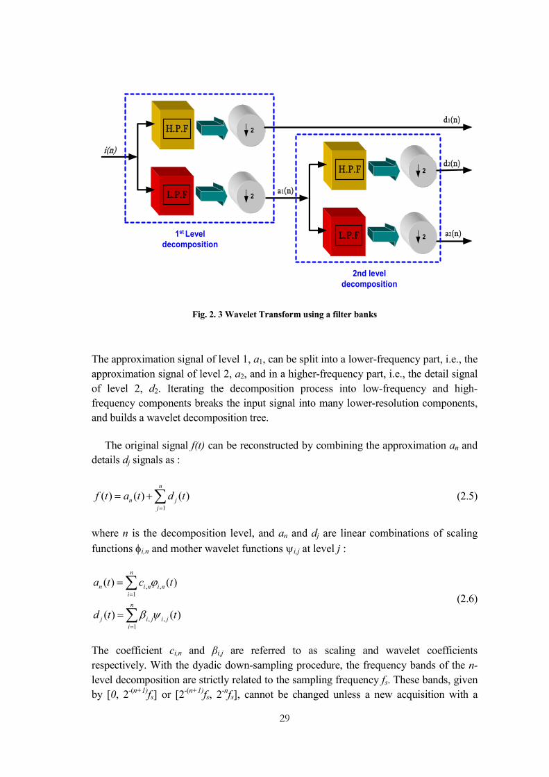
29

2

2

H.P.F

L.P.F

2

2

H.P.F

L.P.F

d1(n)

a1(n)

a2(n)

d2(n)

i(n)

1st Leveldecomposition

2nd leveldecomposition

Fig. 2. 3 Wavelet Transform using a filter banks

The approximation signal of level 1, a1, can be split into a lower-frequency part, i.e., the

approximation signal of level 2, a2, and in a higher-frequency part, i.e., the detail signal

of level 2, d2. Iterating the decomposition process into low-frequency and high-

frequency components breaks the input signal into many lower-resolution components,

and builds a wavelet decomposition tree.

The original signal f(t) can be reconstructed by combining the approximation an and

details dj signals as :

1

( ) ( ) ( )n

n jj

f t a t d t

(2.5)

where n is the decomposition level, and an and dj are linear combinations of scaling

functions i,n and mother wavelet functions i,j at level j :

, ,1

, ,1

( ) ( )

( ) ( )

n

n i n i ni

n

j i j i ji

a t c t

d t t

(2.6)

The coefficient ci,n and βi,j are referred to as scaling and wavelet coefficients

respectively. With the dyadic down-sampling procedure, the frequency bands of the n-

level decomposition are strictly related to the sampling frequency fs. These bands, given

by [0, 2-(n+1)fs] or [2-(n+1)fs, 2-nfs], cannot be changed unless a new acquisition with a

30

different sampling frequency is made, which penalize the memory and latency of

processing.

Discrete Wavelet Transform (DWT) provides greater resolution in time for high

frequency components, and greater resolution in frequency for low frequency

components. So it is particularly suitable for the analysis of transient signals.

Motivated by the above proprieties, DWT have spread in different areas, especially in

the last ten years for power systems quality and protections. Fig. 2.4 show the repartition

of wavelet applications for different power system areas [16].

Fig. 2. 4 Percentage of wavelet applications for different power system areas

2.3 Problematic and developed Diagnosis approach

As already established in chapter 1, the need to develop a new diagnostic approach for

electrical machines operating in time-varying conditions can be formulated with the

following possible improvements over existing techniques: 1) Capability of monitoring

the fault evolution continuously over time under any transient operating condition; 2)

No requirement for speed/slip measurement or estimation; 3) Higher accuracy in

filtering frequency components around the fundamental; 4) Reduction in the likelihood

of false indications by avoiding confusion with other fault harmonics (the contribution

of the most relevant fault frequency components under speed-varying conditions are

clamped in a single frequency band); 5) Low memory requirement due to low sampling

Others 12%

Load forcasting3%

Power system transients

11%

Power system protection

36%

Power system measurement

2%

Power quality32%

Partial discharge4%

31

frequency; 6) Reduction in the latency of time processing (no requirement of repeated

sampling operation).

Electrical machines operate mostly in time-varying conditions. In this context, slip and

speed vary unpredictably, and then chains of fault components related to stator or rotor

faults, such as (fkrs=(s±2k)f)k=0,1,2,…, or (fksr=(12ks)f)k=0,1,2,…, …, are spread in frequency

bands proportional to the speed variation.

In order to carry out a preliminary frequency domain characterization of a stator fault in

time-varying conditions, the fault configuration was emulated in a non-destructive way

using a wound rotor induction machine (WRIM), experimentally mounted in the

laboratory for wind energy application. Since the common effect of both faults is the

unbalance of the corresponding winding impedances, the fault configuration was

emulated by inserting additional resistances in series to the stator phase winding (Radd).

FFT was used to carry out a preliminary characterisation of the stator fault in speed-

varying conditions, to detect experimentally the contribution of the fault components (2-

s)f and (2+s)f under healthy and faulty (Radd=Rs) cases.

Fig. 2.4 shows the experimental rotor modulating signal spectra for large speed transient

under healthy (red line) and stationary stator High-resistance connection (blue line).

Comparing the spectra of the modulating signals, it is evident that a stator asymmetry

produces increments in magnitudes of the components (2-s)f and (2+s)f. Moreover,

being dependent on slip values, under speed varying conditions, the magnitudes of the

above fault components are spread in a bandwidth proportional to the speed variation.

Consequently, the use of Fourier transform in these conditions can lead to an erroneous

diagnosis.

On the other hand, under intermittent stator fault conditions, where the variation of

speed is induced by the degree of the stator unbalance, which justifies the spreading

effect (distortions) observed in Fig. 2.5.

Consequently, the use of Fourier transform in these conditions can lead also to an

erroneous diagnosis. Moreover, time domain information is lost, and then the first point

of the planned improvements “1)” cannot be achieved with this technique.

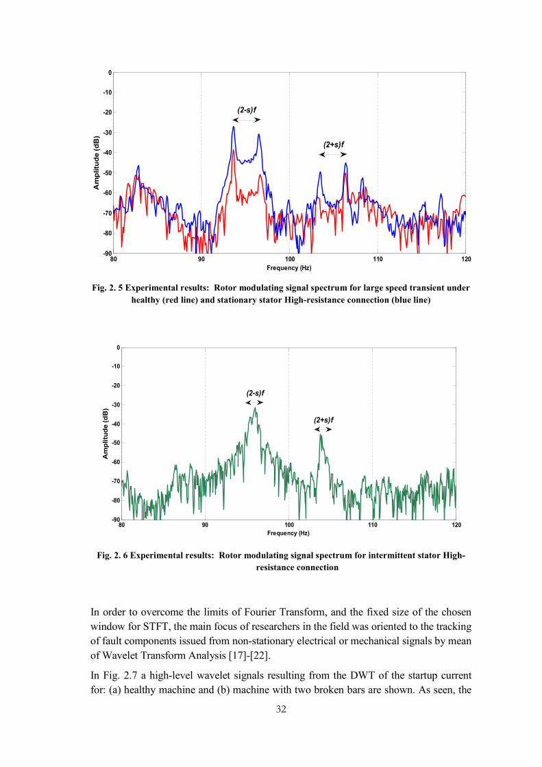
32

Fig. 2. 5 Experimental results: Rotor modulating signal spectrum for large speed transient under

healthy (red line) and stationary stator High-resistance connection (blue line)

Fig. 2. 6 Experimental results: Rotor modulating signal spectrum for intermittent stator High-

resistance connection

In order to overcome the limits of Fourier Transform, and the fixed size of the chosen

window for STFT, the main focus of researchers in the field was oriented to the tracking

of fault components issued from non-stationary electrical or mechanical signals by mean

of Wavelet Transform Analysis [17]-[22].

In Fig. 2.7 a high-level wavelet signals resulting from the DWT of the startup current

for: (a) healthy machine and (b) machine with two broken bars are shown. As seen, the

80 90 100 110 120-90

-80

-70

-60

-50

-40

-30

-20

-10

0

Frequency (Hz)

Am

plitu

de (

dB

)

(2+s)f

(2-s)f

80 90 100 110 120-90

-80

-70

-60

-50

-40

-30

-20

-10

0

Frequency (Hz)

Am

plitu

de (

dB

)

(2-s)f

(2+s)f

33

diagnosis process is based on the comparative study of the different wavelet analysis

under healthy and faulty conditions induced by the spreading effect of the left side band

(1-2s)f characteristic of this fault.

Most of the reported contributions are based on wavelet analysis of currents during the

start-up phase or during any load variation. In this context, the frequency components

are spread in a wide bandwidth as the slip and the speed change considerably. This fact

justify the usage of multi-detail or/and approximation signals resulting from the wavelet

decomposition [20]–[22].

In fact, the different decomposition levels are imposed by the sampling frequency.

However, the dependence on the choice of the sampling frequency and on the capability

of tracking multiple fault frequency components makes difficult to interpret the fault

pattern coming from wavelet signals and increases the diagnosis complexity.

Another issue is that the use of multi-frequency bands for tracking single fault

component subject the process of diagnosis to confusions with other fault components

and then the last four points of the planned improvements “3)-6)”, in the previous

chapter cannot be achieved with a direct use of Discrete Wavelet Transform.

Fig. 2. 7 High-level wavelet signals resulting from the DWT of the startup current for: (a) healthy

machine and (b) machine with two broken bars.

34

Then, a more appropriate technique is needed for providing a reliable diagnosis

procedure to discriminate healthy from faulty conditions under speed or fault varying

conditions.

In the next section, a simple and effective new technique is proposed, providing reliable

information in time-frequency domain for diagnosing electrical machines under time-

varying operating conditions.

2.4 Proposed diagnostic approach

The principal feature of wavelet analysis is its High Multiresolution Analysis HMRA

capability. Wavelet analysis is signal decomposition, using successive combination of

approximation and detail signals. The procedure is repeated until the original signal is

decomposed to a pre-defined J level decomposition. With the well known dyadic down

sampling procedure, frequency bands of each level of decomposition are related to the

sampling frequency. Hence, these bands can’t be changed unless a new acquisition with

different sampling frequency is made. This fact complicates any fault detection based on

DWT, particularly in time-varying condition.

As already analysed in Section 1.2.2, stator fault in induction machines leads to a set of

new components at frequencies (fkss=(1-2k)f)k=0,1,2,… in the stator currents and

(fkrs=(s±2k)f)k=0,1,2,… in the rotor currents (in case of WRIM where rotor quantities are

accessible). Then typically, in case of stator faults, the amplitudes of the sideband

components of a phase current are monitored in order to sense their variation in steady

state conditions. Fig. 2.8 illustrates an extension of the propagation mechanism

corresponding to the evolution of the aforementioned fault components in frequency

domain (Section 1.2.2), to time-frequency domain. The periods of the fault harmonics

are shown on the x-axis, ordered according to the propagation mechanism, whereas the

corresponding frequencies are shown on the y-axis.

Similar considerations can be done for a rotor dissymmetry. In this case, a set of fault

components at frequencies (fksr=(12ks)f)k=0,1,2,… appears in the spectrum of the stator

currents and new fault components at frequencies (fkrr=(1+2k)sf)k=0,1,2,… appear in the

spectrum of rotor currents. The corresponding extension of the propagation

mechanism from frequency (section 2.2.2) to time frequency domain is illustrated by

Fig. 2.9.

35

Fig. 2. 8 Time-frequency propagation of a stator fault. The minus sign (–) identifies current inverse

sequence components

Fig. 2. 9 Time-frequency propagation of a rotor fault. The minus sign (–) identifies current

inverse sequence components

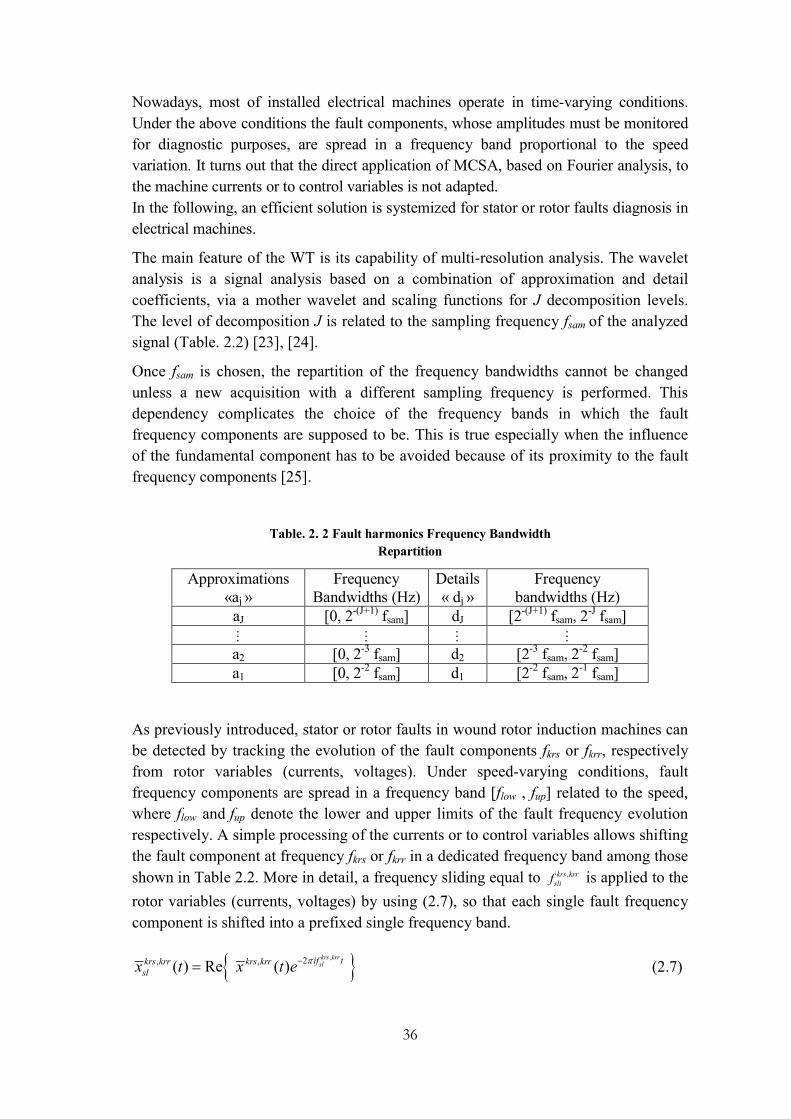
36

Nowadays, most of installed electrical machines operate in time-varying conditions.

Under the above conditions the fault components, whose amplitudes must be monitored

for diagnostic purposes, are spread in a frequency band proportional to the speed

variation. It turns out that the direct application of MCSA, based on Fourier analysis, to

the machine currents or to control variables is not adapted.

In the following, an efficient solution is systemized for stator or rotor faults diagnosis in

electrical machines.

The main feature of the WT is its capability of multi-resolution analysis. The wavelet

analysis is a signal analysis based on a combination of approximation and detail

coefficients, via a mother wavelet and scaling functions for J decomposition levels.

The level of decomposition J is related to the sampling frequency fsam of the analyzed

signal (Table. 2.2) [23], [24].

Once fsam is chosen, the repartition of the frequency bandwidths cannot be changed

unless a new acquisition with a different sampling frequency is performed. This

dependency complicates the choice of the frequency bands in which the fault

frequency components are supposed to be. This is true especially when the influence

of the fundamental component has to be avoided because of its proximity to the fault

frequency components [25].

Table. 2. 2 Fault harmonics Frequency Bandwidth

Repartition

Approximations «aj »

Frequency Bandwidths (Hz)

Details « dj »

Frequency bandwidths (Hz)

aJ [0, 2-(J+1) fsam] dJ [2-(J+1) fsam, 2-J fsam]

a2 [0, 2-3 fsam] d2 [2-3 fsam, 2-2 fsam] a1 [0, 2-2 fsam] d1 [2-2 fsam, 2-1 fsam]

As previously introduced, stator or rotor faults in wound rotor induction machines can

be detected by tracking the evolution of the fault components fkrs or fkrr, respectively

from rotor variables (currents, voltages). Under speed-varying conditions, fault

frequency components are spread in a frequency band [flow , fup] related to the speed,

where flow and fup denote the lower and upper limits of the fault frequency evolution

respectively. A simple processing of the currents or to control variables allows shifting

the fault component at frequency fkrs or fkrr in a dedicated frequency band among those

shown in Table 2.2. More in detail, a frequency sliding equal to ,krs krrslif is applied to the

rotor variables (currents, voltages) by using (2.7), so that each single fault frequency

component is shifted into a prefixed single frequency band.

,2, ,( ) Re ( )krs krr

slif tkrs krr krs krrslx t x t e (2.7)

37

where ,krs krrx is the rotor current or voltage space vector, to be analyzed. Then, the

discrete WT is applied to the resulting signal ,krs krrslx to extract the fault signature in the

frequency band that has been chosen.

As illustrated by Fig. 2.10, the DWT divides the frequency content of the original

signal into logarithmically spaced frequency bands. The approximation aJ and detail dJ

have the same frequency bandwidth, equal to fsam/2J+1. Thanks to its proximity to 0 Hz,

the approximation aJ is less subject to overlapping effect than detail signals and hence is

more suitable for fault analysis [23], [26]. Consequently, the frequency bands

]2,0[ )1(sam

J f are chosen to track the main fault components.

an

dn

dn-1

d1

[0:fs/2n+1] [f

s/2n+1:f

s/2n] [f

s/2n:f

s/2n-1] [f

s/22:f

s/2]

Freq. (Hz)

Fig. 2. 10 The DWT filtering process for decomposition of signal into predetermined frequency bands

Being related to the sampling frequency fsam, the level J of decomposition has to be

chosen in such a way to satisfy the following criterion:

( 1)2 Jup low samf f f (2.8)

Condition (2.8) means that the size of the frequency bandwidth in which the fault

frequency component evolves should be smaller than the bandwidth related to the

approximation signal aJ. Since flow and fup may be affected by uncertainties due to speed

ripples or noise, it is convenient to introduce a tolerance factor , slightly greater than

one, to avoid false alarms after the fault quantification process.

Thus, the level of decomposition is chosen in order to satisfy the following constraint:

log /1

log(2)

sam up lowf f fJ

(2.9)

Once the decomposition level has been chosen, the value of the sliding frequency fsli can

be computed as follows:

12 / 2J

sli low up samf f f f (2.10)

38

With regard to the type of mother wavelet, the use of a low-order Daubechies mother

wavelet (db10) has already provided satisfactory results.

Recently, a high order mother wavelet has been recommended to minimize the

overlapping effect between adjacent frequency bandwidths, and it has already been

tested for rotor broken bars detection [24], [26]. Several types of mother wavelets such

as Daubechies, Coiflet, and Symlet have been tested. Regardless of different properties,

the qualitative analysis of the results has shown that no significant advantages appeared

[27]. The 40th order Daubechies mother wavelet (db40) was adopted in order to

minimize the overlapping effect between adjacent frequency bands related to detail d8

and approximation a8.

Once the state of the machine has been diagnosed, a quantitative evaluation of the fault

degree is necessary. For this purpose, the fault indicator mPaj at different resolution

levels j has been introduced:

2

1

1( , ) ( )

n

j jn

mPa I V a nn

(2.11)

where aj(n) is the approximation signal of interest, Δn denotes the number of samples and j the decomposition level.

The fault indicator is periodically calculated over time, every n sampling period and

over a time interval including the latter n samples. This process is shown in Fig. 2.11.

The values of n and n were chosen according to the desired time sensitivity needed to observe the fault evolution. When the fault occurs, the signal energy distribution changes due to the presence of the fault frequency component. Hence, the energy excess confined in the approximation signal may be considered as a fault indicator in case of stator or rotor unbalances.

''a

j''

sign

al

Time

Samples

n

n

TIN=1

TIN=2

TIN=3

''a

j''

sig

na

lse

qu

en

ces

Fig. 2. 11 Principle of time interval calculation as a function of the Time Interval Number (TIN)

39

2.5 Conclusion

The problematic of signal processing techniques used for electrical machine diagnosis

operating in time-varying conditions was firstly analyzed in this chapter. Then, a new

effective method is completely described and systematized in order to achieve the

different open points established in the previous chapter providing:

- Capability of monitoring the fault evolution continuously over time under any

transient operating condition;

- Speed/slip measurement or estimation is not required;

- Higher accuracy in filtering frequency components around the fundamental;

- Reduction in the likelihood of false indications by avoiding confusion with other

fault harmonics (the contribution of the most relevant fault frequency components

under speed-varying conditions are clamped in a single frequency band);

- Low memory requirement due to low sampling frequency;

- Reduction in the latency of time processing (no requirement of repeated sampling

operation).

40

REFERENCES

[1] T. Chow and S. Hai, "Induction machine fault diagnostic analysis using wavelet

technique", IEEE Transactions Industrial Electronics, Vol. 51, N°. 3, pp. 558–

565, Jun. 2004.

[2] Hua Su, Kil To Chong, "Induction Machine Condition Monitoring Using Neural

Network Modeling'', IEEE Transactions Industrial Electronics, Vol. 54, Issue 1,

pp. 241 – 249, Feb. 2007.

[3] R.J. Romero-Troncoso, R.A. Osornio-Rios, E. Cabal-Yepez, J.J. Rangel-

Magdaleno and L.M. Contreras-Medina, "Novel Methodology for Online Half-

Broken-Bar Detection on Induction Motors", IEEE Transactions on

Instrumentation and Measurement, Vol. 58, N°. 5, May. 2009.

[4] H. Henao, C. Martis, G.A. Capolino, "An Equivalent Internal Circuit of the

Induction Machine for Advanced Spectral Analysis", IEEE Transactions on

Industry Applications, Vol. 40, N°. 3, May/June 2004.

[5] K. Bacha, H. Henao, M. Gossa, G.A. Capolino, "Induction machine fault

detection using stray flux EMF measurement and neural network-based

decision", Electric Power Systems Research, Vol. 78, pp. 1247–1255, 2008.

[6] J. S. Hsu, "Monitoring of defects in induction motors through airgap torque

observation", IEEE Trans. Ind. Appl., vol. 31, no. 5, pp. 1016–1021, Sep./Oct.

1995.

[7] C. Kral, R. S. Wieser, F. Pirker, and M. Schagginger, "Sequences of field-

oriented control for the detection of faulty rotor bars in induction machines-the

Vienna Monitoring Method", IEEE Transactions Industrial Electronics, Vol. 47,

N°. 5, pp. 1042–1050, Oct. 2000.

[8] D. Casadei, F. Filippetti, C. Rossi, A. Stefani "Closed Loop Bandwidth Impact

on Doubly Fed Induction Machine Asymmetries Detection Based on Rotor

Voltage Signature Analysis", 43rd International Universities Power Engineering

Conference, UPEC 2008.


"Doubly Fed Induction Machines Diagnosis Based on Signature Analysis of

Rotor Modulating Signals", IEEE Transactions on Industry Application, Vol. 44,

N° 6, Nov/Dec 2008.

[10] Frédéric Truchetet, « Ondelettes pour le signal numérique », Hermes, Paris

1998, ISBN 2-86601-672-6.

[11] S.G. Mallat, "A Theory for Multiresolution Signal Decomposition: The Wavelet

Representation", IEEE Transactions on pattern analysis and machine

intelligence. Vol. II, N°. 7. July 1989.

41

[12] R.J.E. Merry, “Wavelet Theory and Applications A literature study”, DCT

2005.53, Eindhoven, June 7, 2005.

[13] I. Daubechies, "Where do Wavelets Come From? A personal Point of view",

Proceedings of the IEEE, Vol. 84, N°. 4, April 1996.

[14] G.T. Heydet, P.S. Fjeld, C.C. Liu, D. Piercel, L. TU, G. Hensley, "Applications

of the windowed FFT to Electric power quality assessment", IEEE Transactions

on Power Delivery, Vol. 14, N° 4, pp.1411-1416, Oct. 1999.

[15] R. Pineda-Sanchez, M. Riera-Guasp, M. Roger-Folch, J. Hurtado-Perez, E.

Perez-Cruz, J. ''Improved Resolution of the MCSA Method Via Hilbert

Transform, Enabling the Diagnosis of Rotor Asymmetries at Very Low Slip'',

IEEE Transactions on Energy Conversion Vol. 24, Issue 1, pp. 52 – 59, March

2009.

[16] R. de C. Fernandez, H. N. Diaz Rojas, "An overview of wavelet transforms

application in power systems", 14th Power Systems Computation Conference,

Session 1, paper 6, Seville, 2002.

[17] J. Antonino-Daviu, P. Jover Rodriguez, M. Riera-Guasp, M. Pineda Sanchez,

and A. Arkkio, “Detection of combined faults in induction machines with stator

parallel branches through the DWT of the startup current,” Mech. Syst. Signal

Process., vol. 23, no. 7, pp. 2336–2351, Oct. 2009.

[18] J. Pons-Llinares, J. A. Antonino-Daviu, M. Riera-Guasp, M. Pineda-Sanchez,

and V. Climente-Alarcon, “Induction motor diagnosis based on a transient

current analytic wavelet transform via frequency B-splines,” IEEE Trans. Ind.


[19] A. Gandhi, T. Corrigan, and L. Parsa, “Recent advances in modeling and online

detection of stator interturn faults in electrical motors,” IEEE Trans. Ind.


[20] A. Ordaz-Moreno, R. J. Romero-Troncoso, J. A. Vite-Frias, J. R. Rivera-Gillen,

and A. Garcia-Perez, “Automatic online diagnosis algorithm for broken-bar

detection on induction motors based on discrete wavelet transform for FPGA

implementation,” IEEE Trans. Ind. Electron., vol. 55, no. 5, pp. 2193–2202,

May 2008.




Sep. 2011.

[22] J. Antonino-Daviu, S. Aviyente, E. G. Strangas, and M. Riera-Guasp, “Scale

Invariant Feature Extraction Algorithm for the Automatic Diagnosis of Rotor

Asymmetries in Induction Motors”, IEEE Trans. Ind. Inf., vol. 9, no. 1, pp. 100–

108, Feb. 2013.

42

[23] T. K. Sarkar, C. Su, R. Adve, M. S. Palma, L. G. Castillo, and R. Boix, “A

tutorial on wavelets from an electrical engineering perspective, Part 1: Discrete

wavelet techniques,” IEEE Antennas Propag. Mag., vol. 40, no. 5, pp. 49–68,

Oct. 1998.

[24] M. Riera-Guasp, J.A. Antonino, J. Roger-Folch, M.P. Molina, “The use of the

wavelet approximation signal as a tool for the Diagnosis and quantification of

Rotor Bar Failures, ” IEEE Trans. Ind. App., vol. 44, no. 3, pp. 716–726,

May./Jun. 2008.

[25] M.R. Guasp, J.A. Daviu, M.P. Sanchez, R.P. Panadero, J.P. Cruz, “A general

approach for the transient detection of slip-dependent fault components based on

the discrete wavelet transform,” IEEE Trans. Ind. Elec., vol. 55, no. 12, pp.

4167–4180 Dec. 2008.

[26] S. H. Kia, H. Henao, and G. A. Capolino, “Diagnosis of broken-bar fault in

induction machines using discrete wavelet transform without slip estimation,”

IEEE Trans. Ind. Appl., vol. 45, no. 4, pp. 1395–1404, Jul./Aug. 2009.

[27] J. Antonino-Daviu, M. Riera-Guasp, J. Roger-Folch, F. Martínez-Giménez, A.

Peris, “Application and optimization of the discrete wavelet transform for the

detection of broken rotor bars in induction machines,” Appl. Comp. Harmon.

Anal., vol. 21, no. 2, pp. 268–279, Sep. 2006.

44

CHAPTER 3 : ANALYSIS OF STATOR

AND ROTOR FAULTS IN WOUND

ROTOR INDUCTION MACHINES

3.1 Introduction ........................................................................................................................... 45 3.2 System description ................................................................................................................ 45

3.2.1 WRIM Control system ................................................................................................. 45 3.2.2 Experimental system ..................................................................................................... 49

3.3 Results ..................................................................................................................................... 51 3.3.1 Fault detection under speed-varying condition........................................................ 51

3.3.1.1 Stator dissymmetry detection .......................................................................... 52 3.3.1.2 Rotor dissymmetry detection .......................................................................... 55

3.3.2 Fault detection under fault-varying conditions ........................................................ 56 3.3.2.1 Stator progressive dissymmetry detection ..................................................... 58 3.3.2.2 Rotor progressive dissymmetry detection ..................................................... 60

3.4 Fault quantification ............................................................................................................... 60 3.5 Conclusion ............................................................................................................................. 65 References ............................................................................................................................................ 66

45

3.1 Introduction

In this chapter, the proposed diagnosis technique presented in Chapter 2 is validated for

the detection of electrical faults in three-phase wound-rotor induction machines

(WRIMs). In the considered application, the rotor windings are supplied by a static

converter for the control of active and reactive power flows exchanged between the

machine and the electrical grid. In this application, the proposed diagnosis approach was

applied for processing the rotor-voltage commands under time-varying conditions. Thus,

the time evolution of fault components can be effectively analyzed. Moreover, the

relevance of the fault components computed from rotor voltages in comparison to those

coming from rotor currents under closed-loop operation is evaluated. Results issued

from the quantitative evaluation process of the fault extend issued from the wavelet

analysis are presented showing accurate stator- or rotor-fault detection. Simulation and

experimental results show the validity of the proposed method, leading to an effective

diagnosis procedure for both stator and rotor electrical faults in WRIMs.

3.2 System description

3.2.1 WRIM Control system

In this application, the wound-rotor induction machine is fed by a back-to-back

converter on the rotor side and with the stator directly connected to the grid. A Stator

Flux Oriented Control (SFOC) system is implemented to regulate rotor currents, in order

to control separately the active and reactive power on the stator side [1]-[3]. In the dq

reference frame rotating synchronously with the stator flux, the stator voltages and

fluxes can be written as follows:

dsds s ds qs

dv R i

dt

(3.1)

qs

qs s qs ds

dv R i

dt

(3.2)

ds s ds m drL i L i (3.3)

0qs s qs m qrL i L i (3.4)

The above equations mean that the d-axis is in phase with stator-flux vector. In steady-

state conditions, by neglecting the stator-phase resistance and by introducing the

magnetizing current /ms s mi L the stator voltage and current components become:

0dsv (3.5)

46

qs s dsv v (3.6)

mds dms dr

s

Li i i

L (3.7)

mqs qr

s

Li i

L (3.8)

The active and reactive power are expressed as:

3

2s ds ds qs qsP v i v i . (3.9)

3

2s qs ds ds qsQ v i v i . (3.10)

By introducing (3.5)–(3.8) in (3.9) and (3.10), it is possible to rewrite the active and

reactive power as function of stator-voltage and rotor-current components as:

3

2m

s s qr

s

LP v i

L (3.11)

3

2 2sm

s s dr

s m

vLQ v i

L f L

(3.12)

Using (3.11) and (3.12) and assuming constant stator-voltage magnitude |V S| and

frequency f, it is possible to consider the stator active power proportional to the q-axis

rotor-current component iqr and the stator reactive power related to the d-axis rotor-

current component idr.

The DFIM control system (Fig. 3.1) is based on two cascaded loops. The outer loop is

dedicated to the stator active and reactive power control, whereas the inner loop is

related to the control of the dq components of the rotor current. Since the control system

is symmetrical, the PI regulators have the same parameters for the d- and the q-axes

loops.

The two PI regulators of the outer loop are used to determine the dq components of the

rotor-current references on the basis of the active and reactive power errors.

The two PI regulators of the inner loop are used to determine the dq components of the

rotor modulating signals using the dq rotor-current errors as input variables.

The transformations from three-phase quantities in a dq stationary reference frame and

the inverse transformations are performed by the blocks D and D−1, respectively. Being

θ and θr, the stator-flux-phase and the rotor-position angles, respectively, the block T(θ)

represents the transformation from a stationary reference frame to a synchronous

rotating reference frame, as well as the block T(θ − θr) represents the transformation

47

from a rotor reference frame to a synchronous reference frame. The blocks T−1(θ) and

T−1(θ − θr) represent the corresponding inverse transformations.

The control algorithm computes the phase angle θ of the stator-flux vector using the

components of the magnetizing current space vector isdms, is

qms in the stator reference

frame as:

arctansqms

sdms

i

i

(3.13)

In order to increase the accuracy in the computation of the angle θ, a complex digital

filter is applied to detect the fundamental frequency component of the magnetizing-

current space vector smsi .

The transfer function of the digital filter in terms of Laplace transform is derived as

follows.

In the synchronous reference frame which rotates at a constant angular speed 2πf, the

filtered magnetizing-current vector ( )ms fili is obtained by applying a first-order low-pass

filter to the magnetizing-current vector msi , yielding

( )

1

1ms fil msi i

s

(3.14)

where τ is the low-pass-filter time constant. The magnetizing-current vector in the

synchronous reference frame is related to the magnetizing-current vector in the

stationary reference frame by the following relationship:

sjsms msi i e (3.15)

By introducing (3.15) in (3.14), the equation of the filtered magnetizing-current vector

in the stationary reference frame becomes:

( )

1

1 ss s

ms fil msi ij

(3.16)

where ω is the stator-flux angular frequency, assumed constant and equal to 2πf[rad/s].

Then, the dq components of the magnetizing-current vector can be derived from (3.16),

yielding:

( ) 2 2 2

1 s

1 s

s smsd qmss

msd fil

i ii

(3.17)

( ) 2 2 2

1 s

1 s

s sdms qmss

qms fil

i ii

(3.18)

48

Equations (3.13), (3.17) and (3.18) are implemented in the block msi of Fig. 3.1.

The block Act–React of Fig. 3.1 calculates the active and reactive power by using (3.9)

and (3.10).

For computer simulations, an analytical three-phase model of the WRIM and its control

system has been implemented in Matlab-Simulink. As detailed in Appendix.1 a transient

general model was adopted for wind power generation systems. In this model,

coordinate transformations are not utilized and equations are written for every stator and

rotor phase. Moreover stator variables and parameters are referred to the stator reference

frame, whereas rotor variables and parameters are referred to the rotor reference frame.

This means that every parameter present in the model is the true physical parameter of

every single phase winding. This choice was done since in a wound rotor induction

machines both rotor and stator terminals are accessible allowing the measurement of all

the necessary phase parameters [3]-[4]. The model was modified in order to manage all

the machine parameters for emulating different configurations of stator or rotor fault

varying conditions.

Fig. 3. 1 Block-scheme representation of the complete WRIM control system

DFIM

D-1

back-to-back

D

T-1(-r)

T(r)-1

T()

Ims-

PI

PI

PI

PI

T(-r)

Act-React

*arV*brV*crV

asi

bsi

csi

s

1

r

rqrV

rdrV

rqri

rdri

sqsi

sdsi

sqri

sdri

m

s

L

L

sqmsi

sdmsi

r r

*qrV

*drV

r

*qri

*dri

qri

dri

*sP

*sQ

qsi

sP sQ

sP sQ

r

D T()

sqsv

sdsv

asv

bsv

csv

qsv

dsv

dsi

m

s

L

L

D

ari

bri

cri

49

3.2.2 Experimental system

The experimental setup (Fig. 3.2) consists of a 5.5-kW 220- V/ 380-V 50-Hz four-pole

WRIM connected to a pulse width modulated back-to-back power converter on the rotor

side. The generator is driven by a 9-kW dc motor fed by a commercial speed-controlled

dc/dc converter. The field-oriented control for the WRIM has been implemented on a

dSPACE DS1103 board. Since the speed of the WRIM is not fixed by the control

system (because the WRIM set points are the active and reactive powers), the rotor

speed is determined by the dc motor and can be varied by acting on the corresponding

set point.

For the assessment of the fault diagnosis algorithm, the grid voltages, the rotor-side line

currents, the reference rotor voltages, the rotor and stator currents, and the rotor speed

are sampled at 3.2 kHz with a data acquisition window of 10 s. Finally, the frequency

bandwidth of the current loops has been set to 100 Hz. Other parameters of the

experimental setup, used also for the simulations, have been reported in Tables. 3.1-3.3.

Since the common effect of both stator and rotor faults is the imbalance of the

corresponding winding impedances, the fault configurations have been emulated in a

nondestructive way by increasing the stator or the rotor phase resistances with additive

components (Radd). During the tests, active and reactive power set points at the stator

side are kept equal to 5.5 kW and 4.1 kVA, respectively.

(a)

50

(b)

c)

Fig. 3. 2 Experimental set-up. a) Power converter cabinet. b) WRIM and prime mover. c)

Schematic diagram of the test bench and position of the current and voltage sensors.

Table. 3. 1 WRIM parameters

Parameter Value

Rated power kW 5.5

Rated stator/ rotor voltage V 380/186

Rated frequency Hz 50

Rated speed rpm 1400

Stator phase resistance Ω 0.531

Rotor phase resistance Ω 0.310

Stator inductance H 0.083

Rotor inductance H 0.019

Mutual inductance H 0.038

Pole pairs 2

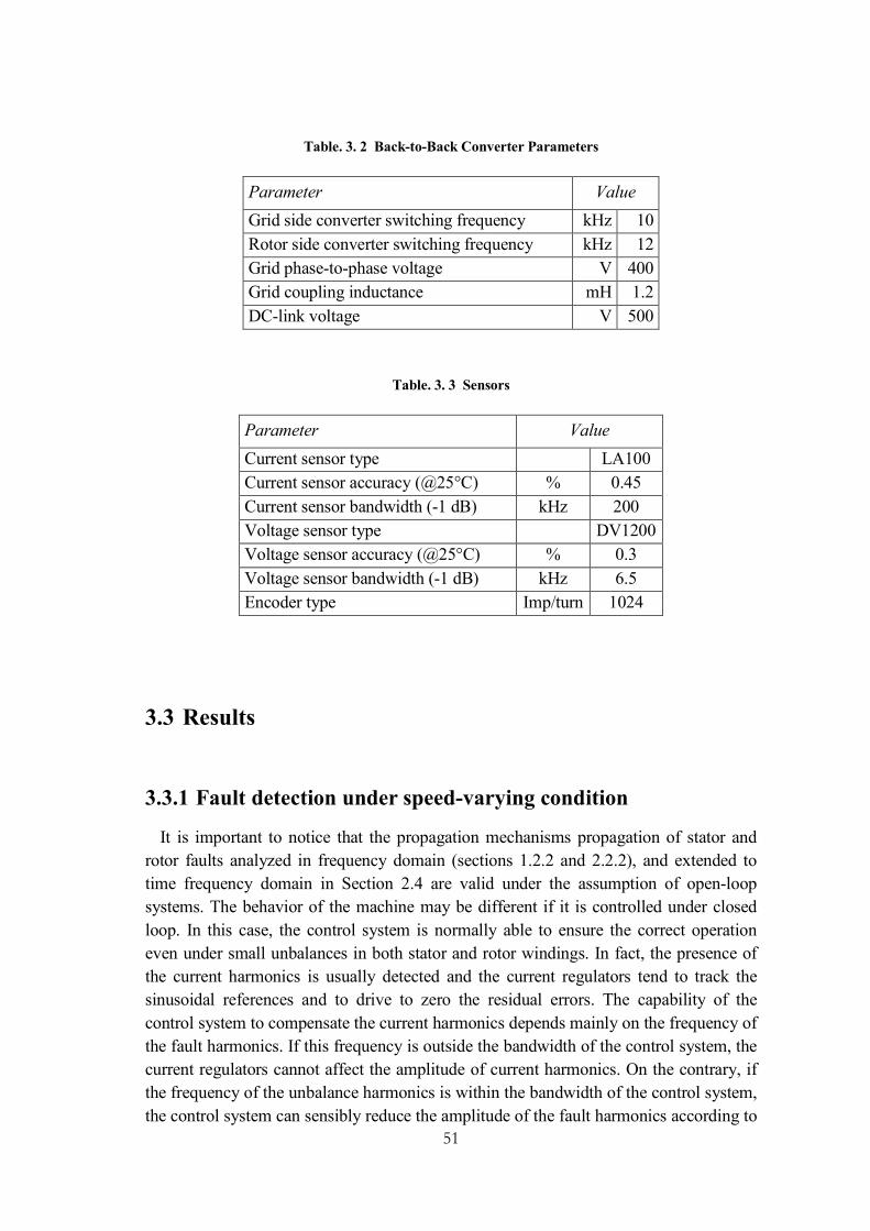
51

Table. 3. 2 Back-to-Back Converter Parameters

Parameter Value

Grid side converter switching frequency kHz 10

Rotor side converter switching frequency kHz 12

Grid phase-to-phase voltage V 400

Grid coupling inductance mH 1.2

DC-link voltage V 500

Table. 3. 3 Sensors

Parameter Value

Current sensor type LA100

Current sensor accuracy (@25°C) % 0.45

Current sensor bandwidth (-1 dB) kHz 200

Voltage sensor type DV1200

Voltage sensor accuracy (@25°C) % 0.3

Voltage sensor bandwidth (-1 dB) kHz 6.5

Encoder type Imp/turn 1024

3.3 Results

3.3.1 Fault detection under speed-varying condition

It is important to notice that the propagation mechanisms propagation of stator and

rotor faults analyzed in frequency domain (sections 1.2.2 and 2.2.2), and extended to

time frequency domain in Section 2.4 are valid under the assumption of open-loop

systems. The behavior of the machine may be different if it is controlled under closed

loop. In this case, the control system is normally able to ensure the correct operation

even under small unbalances in both stator and rotor windings. In fact, the presence of

the current harmonics is usually detected and the current regulators tend to track the

sinusoidal references and to drive to zero the residual errors. The capability of the

control system to compensate the current harmonics depends mainly on the frequency of

the fault harmonics. If this frequency is outside the bandwidth of the control system, the

current regulators cannot affect the amplitude of current harmonics. On the contrary, if

the frequency of the unbalance harmonics is within the bandwidth of the control system,

the control system can sensibly reduce the amplitude of the fault harmonics according to

52

the gain of the control loop at those frequencies. This behavior is due to the current

regulators that naturally applies suitable voltage harmonics to cancel the corresponding

current harmonics. At the same time, torque and speed oscillations are accordingly

damped.

Since the bandwidth of the current loops is usually quite wide, the reduction effect on

the main fault frequencies may be remarkable, and the fault frequencies are expected to

appear in the voltage set-points at the output of the current regulators [5].

In the case of the WRIM-based system of Fig. 3.1, the rotor-current fault frequency

components may become less notable due to the compensating action of the control

system. However, these fault-related frequencies become clearly visible in the

modulating signals of the rotor voltages, which can be considered as a new effective

diagnostic index. In other words, a stator fault is expected to generate a relevant

harmonic at (s-2)f in the spectrum of the rotor voltages, whereas a rotor fault is expected

to generate a negative sequence harmonic at -sf. The detection of the inverse sequence

frequency components at (s-2)f and -sf is possible only by analyzing the rotor voltage

space vector. Initially, the performance of the WRIM has been verified in healthy

condition during a speed transient from 1395 to 1305 r/min. With a sampling frequency

fsam of 3.2 kHz, an eighth-level decomposition (J = 8) has been chosen to track the

components frs = (s − 2)f and frr = −sf in the time domain. The computed values of

frequency sliding are 98.125 and 8.125 Hz, respectively.

3.3.1.1 Stator dissymmetry detection

This fault configuration has been simulated by means of an additional resistance Radd

connected in series with one stator phase winding and equal to the phase resistance Rs.

Rotor currents and voltages, used for space vectors (ir,Vr)rs computation under healthy

and faulty conditions, have been recorded. Simulation results are shown in Figs. 3.3 and

3.4, which compare the WRIM operation in both healthy and fault conditions. Figs. 3.5

and 3.6 show the behavior of the WRIM during the experimental tests under the same

operating conditions.

The contribution of the stator fault component at frequency (s–2)f must be extracted

from both rotor current and voltage space vectors. The 8th-level approximations coming

from the discrete WT of ( )rsslI t and ( )rs

slV t in healthy and fault conditions have been

computed under the assumption of a sliding frequency krsslif equal to 98.125 Hz. In

healthy condition, the approximation a8 does not show any variation. This fact indicates

the absence of any fault component at frequency (s-2)f, in both rotor currents and

voltages, thus leading to diagnose the healthy condition of the WRIM even under speed-

varying operation.

In the case of stator unbalance (Radd=Rs), the approximation a8 issued from rotor

currents analysis does not show any significant change. This is mainly due to the

compensating action of the control system under fault condition [5]. However, for the

53

same stator unbalance, large oscillations appear in the approximation a8 issued from the

rotor voltages. These oscillations have a constant magnitude depending on the unbalance

degree (Radd=Rs). The frequency variations of the oscillations during the transient is due

to the slip-dependency of the fault component at (s-2)f .

As can be seen, this behavior is confirmed not only by the simulation results, but also by

the experimental tests (Figs. 3.5 and 3.6), although in some cases the magnitude

variations have been even greater in the experimental tests compared to what has been

observed in the simulations.

In particular, Fig. 3.6 shows that the ratio between the amplitude of the approximation

signal a8 ( 0.5A) and the amplitude of the current ( 29A) is less than 0.017, whereas

the ratio between the amplitude of the approximation signal a8 (1.2V) and the amplitude

of the voltage (27V before the speed step and 40 V after the speed step) varies from

0.044 to 0.030. In other words, the effect of the unbalance is from two to three times

more visible in the voltage signals than in the current signals.


slV in healthy condition (Radd=0) under speed transient

(simulation results)

0 2 4 6 8 101280

1330

1380

1420- a -

Sp

ee

d (

rpm

)

0 2 4 6 8 101280

1330

1380

1420- b -

Sp

ee

d (

rpm

)

0 2 4 6 8 10

-0.5

0

0.5

- e -

Time (s)

a8

(A

)

0 2 4 6 8 10-3

0

3- f -

Time (s)

a8

(V

)

0 2 4 6 8 10-50

0

50- c -

Cu

rre

nt (A

)

0 2 4 6 8 10-50

0

50- d -

Vo

lta

ge

(V

)

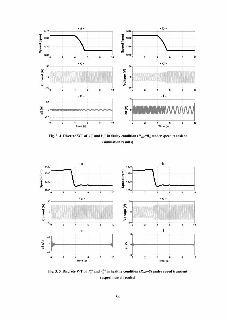
54


slV in faulty condition (Radd=Rs) under speed transient




(experimental results)

0 2 4 6 8 101280

1330

1380

1420- a -

Sp

ee

d (rp

m)

0 2 4 6 8 101280

1330

1380

1420- b -

Sp

ee

d (rp

m)

0 2 4 6 8 10

-0.5

0

0.5

- e -

Time (s)

a8

(A

)

0 2 4 6 8 10-3

0

3- f -

Time (s)a

8 (V

)

0 2 4 6 8 10-50

0

50- c -

Cu

rre

nt

(A)

0 2 4 6 8 10-50

0

50- d -

Vo

lta

ge

(V

)

0 2 4 6 8 101280

1330

1380

1420- a -

Sp

ee

d (

rpm

)

0 2 4 6 8 101280

1330

1380

1420- b -

Sp

ee

d (

rpm

)

0 2 4 6 8 10

-0.5

0

0.5

- e -

Time (s)

a8

(A

)

0 2 4 6 8 10-3

0

3- f -

Time (s)

a8

(V

)

0 2 4 6 8 10-50

0

50- c -

Cu

rre

nt

(A)

0 2 4 6 8 10-50

0

50- d -

Vo

lta

ge

(V

)

55


slV in faulty condition (Radd=Rs) under speed transient


3.3.1.2 Rotor dissymmetry detection

The same process has been repeated for the analysis of a rotor unbalance simulated

by an additive resistance connected in series with a rotor phase and equal to its own

resistance. In order to detect such a fault, the contribution of the rotor fault component at

frequency -sf has to be extracted from the rotor current and voltage space vectors. Rotor

currents and voltages have been recorded for the computation of the space vectors

(ir,Vr)rr in healthy and faulty conditions. The simulation results, shown in Figs. 3.7 and

3.8, show a good agreement with the corresponding experimental tests, shown in Figs.

3.9 and 3.10. With similar considerations as for the stator fault, the signals ( )rrslI t and

( )rrslV t have been computed by using krs

slif =8.125 Hz. The aim of this pre-processing

operation is to identify the contribution of the negative sequence frequency -sf in the

frequency band of the 8th approximation signal. Approximations a8 coming from the

discrete WT of signals ( )rrslI t and ( )rr

slV t under both healthy and faulty conditions have

been computed. In healthy condition, the approximation a8 does not show any

oscillation since the fault components at frequency -sf in both rotor currents and voltages

are not involved. This fact indicates a reliable diagnosis of healthy condition for the

WRIM under speed-varying operation.

Under rotor unbalance (Radd=Rr), the same conclusion as for a stator unbalance has been

obtained. The approximation a8 coming from the rotor voltages shows large amplitude

0 2 4 6 8 101280

1330

1380

1420- a -

Sp

ee

d (

rpm

)

0 2 4 6 8 101280

1330

1380

1420- b -

Sp

ee

d (

rpm

)0 2 4 6 8 10

-0.5

0

0.5

- e -

Time (s)

a8

(A

)

0 2 4 6 8 10-3

0

3- f -

Time (s)a

8 (

V)

0 2 4 6 8 10-50

0

50- c -

Cu

rre

nt

(A)

0 2 4 6 8 10-50

0

50- d -

Vo

lta

ge

(V

)

56

variations reflecting the presence of the fault frequency component -sf. Despite the

speed transient, the oscillations reproducing the fault frequency evolution -sf are still

significant. On the contrary, the variation of a8 calculated for the rotor currents is small

compared to the amplitude of the currents (Fig. 3.8). Experimental results under healthy

and faulty (Rradd=Rr) conditions have confirmed this behavior (Figs. 3.9 and 3.10). More

accurately, the contribution of the negative sequence at the frequency -sf under a rotor

unbalance coming from the rotor voltages is more important than the corresponding one

coming from rotor currents.

In conclusion, the experimental results are in total agreement with the simulation, thus

proving the effectiveness of the proposed approach for the diagnosis of electrical rotor

faults in a WRIM.




3.3.2 Fault detection under fault-varying conditions

The results obtained in Section IV prove that the wavelet signal a8 is sensitive enough to

diagnose either stator or rotor winding unbalances in any WRIM operating conditions.

This fact confirms the validity of the proposed technique applied to rotor voltages even

in presence of slip variations.

In this section, the sensitivity of the proposed diagnostic technique is evaluated by the

analysis of progressive stator and rotor winding unbalances. These fault configurations

have been simulated through a ramp of resistance increment from Radd =0 to Radd=1.3Rs

or Radd=1.3Rr under stator or rotor progressive unbalance respectively. The experimental

0 2 4 6 8 101280

1330

1380

1420- a -

Sp

ee

d (

rpm

)

0 2 4 6 8 101280

1330

1380

1420- b -

Sp

ee

d (

rpm

)

0 2 4 6 8 10-50

0

50- c -

Cu

rre

nt

(A)

0 2 4 6 8 10-50

0

50- d -

Vo

lta

ge

(V

)

0 2 4 6 8 10

-0.5

0

0.5

- e -

Time (s)

a8

(A

)

0 2 4 6 8 10-3

0

3- f -

Time (s)

a8

(V

)

57

set-up has been designed to emulate these situations by inserting an external variable

resistance in series to a stator or a rotor phase. For the above listed tests, the WRIM

operates in steady-state condition at the rated speed of 1400rpm.


slV in faulty condition (Radd=Rr) under speed transient





0 2 4 6 8 101280

1330

1380

1420- a -

Sp

eed

(rp

m)

0 2 4 6 8 101280

1330

1380

1420- b -

Sp

eed

(rp

m)

0 2 4 6 8 10-50

0

50- c -

Cu

rren

t (A

)

0 2 4 6 8 10-50

0

50- d -

Vo

lta

ge

(V

)

0 2 4 6 8 10

-0.5

0

0.5

- e -

Time (s)

a8

(A

)

0 2 4 6 8 10-3

0

3- f -

Time (s)

a8

(V

)

0 2 4 6 8 101280

1330

1380

1420- a -

Sp

eed

(rp

m)

0 2 4 6 8 101280

1330

1380

1420- b -

Sp

eed

(rp

m)

0 2 4 6 8 10-50

0

50- c -

Cu

rren

t (A

)

0 2 4 6 8 10-50

0

50- d -

Vo

ltag

e (

V)

0 2 4 6 8 10

-0.5

0

0.5

- e -

Time (s)

a8

(A

)

0 2 4 6 8 10-3

0

3- f -

Time (s)

a8

(V

)

58


slV in faulty condition (Radd=Rr) under speed transient


3.3.2.1 Stator progressive dissymmetry detection

The stator resistance has been linearly varied in simulation from Radd=0 to Radd=1.3Rs.

At rated speed, the value of krsslif used for the computation of ( )sr

slV t is -99.79 Hz. The

simulation result of Fig. 3.11 has been confirmed by experimental tests in the same

conditions (Fig. 3.12). During the first time interval (from t=0s to t ≈ 2s) under healthy

condition, the three-phase rotor voltages are balanced and sinusoidal. For this time

interval, the 8th approximation signal, representative of the stator fault component at

the frequency (s-2)f, does not show any variation. During the ramp variation of the

stator resistance emulating the winding fault, the rotor phase voltages are balanced,

although progressive distortions appear, which indicate the increasing contribution of

the fault component at frequency (s-2)f. As can be seen, the progressive stator

unbalance is visible in the approximation signal a8, showing a proportional increase of

its magnitude. Hence, the trend of the approximation signal is related to the fault

component evolution at frequency (s-2)f. The experimental tests corroborate the

simulation result and prove the effectiveness of the proposed technique.

0 2 4 6 8 101280

1330

1380

1420- a -

Sp

eed

(rp

m)

0 2 4 6 8 101280

1330

1380

1420- b -

Sp

eed

(rp

m)

0 2 4 6 8 10-50

0

50- c -

Cu

rren

t (A

)

0 2 4 6 8 10-50

0

50- d -

Vo

ltag

e (

V)

0 2 4 6 8 10

-0.5

0

0.5

- e -

Time (s)

a8

(A

)

0 2 4 6 8 10-3

0

3- f -

Time (s)

a8

(V

)

59

Fig. 3. 11 Discrete WT of krsslV under progressive stator unbalance condition (simulation results)



0 1 2 3 4 5 6 7 8 9 10-40

0

40- a -

Vo

lta

ge

s (

V)

0 1 2 3 4 5 6 7 8 9 10

-4

-2

0

2

4

- b -

Time (s)

a8

(V

)

0 0.1 0.2 0.3 0.4 0.5-40

0

40

9.5 9.6 9.7 9.8 9.9 10-40

0

40

0 1 2 3 4 5 6 7 8 9 10-40

0

40- a -

Vo

lta

ge

s (

V)

0 1 2 3 4 5 6 7 8 9 10

-4

-2

0

2

4

- b -

Time (s)

a8 (

V)

0 0.1 0.2 0.3 0.4 0.5-40

0

40

9.5 9.6 9.7 9.8 9.9 10-40

0

40

60

3.3.2.2 Rotor progressive dissymmetry detection

The rotor resistance has been progressively varied in simulation from Radd=0 to

Radd=1.3Rr. At rated speed, the value of krrslif to compute ( )rs

slV t is -6.45 Hz. The

simulation result (Fig. 3.13) has been confirmed by experimental tests in the same

conditions (Fig. 3.14). As it can be seen, in healthy condition (from t=0s to t ≈ 2s) the

three-phase rotor voltages are quite balanced and sinusoidal. The corresponding

approximation signal a8 does not show any particular oscillation during the two first

seconds. When the rotor fault occurs, the three-phase rotor voltages are almost

sinusoidal but become progressively unbalanced as long as the contribution of the fault

frequency component -sf increases. This is clearly reflected by the progressive distortion

of the approximation a8, allowing to diagnose the rotor windings degradation. In

conclusion, the experimental results are in complete agreement with the simulations.

3.4 Fault quantification

Once the state of the machine has been diagnosed, a quantitative evaluation of the

fault degree is necessary. The fault indicator is periodically calculated over time, every

δn sampling period, and over a time interval including the latter Δn samples. This

process is illustrated by Fig. 2.11.

During the experimental tests, the time interval between two consecutive calculations of

the fault indicator was 125 ms, and the length of the time window for the calculation of

the fault indicator was 2000 ms. Since the sample frequency was 3200 Hz, the number

of samples between two consecutive calculations of the fault indicator was δn = 125

10−3 · 3200 = 400, and the length of the sequence of samples was Δn = 2000 10−3 · 3200

= 6400. The values of δn and Δn were chosen according to the desired time sensitivity to

observe the fault evolution.

When the fault occurs, the signal energy distribution changes due to the presence of

the fault frequency component. Hence, the energy excess confined in the

approximation signal may be considered as a fault indicator in case of stator or rotor

unbalances.

The trends of the fault indicators mPa8(I) and mPa8(V) corresponding to the

simulation results depicted in Figs. 3.3 and 3.4 were computed under healthy and faulty

conditions and are shown in Fig. 3.15. In healthy conditions (Radd=0), and under large

range of speed variations, mPa8(I) and mPa8(V) are practically constant. Consequently,

the indicator values for the healthy WRIM can be assumed as a baseline to set the

threshold to discriminate healthy from stator unbalance conditions.

Under faulty condition (Radd=Rs), mPa8(I) does not show any significant variation. As

previously discussed, this is due to the compensating effect of the control system.

However, mPa8(V) shows a significant increase. The large energy deviation observed in

faulty condition proves the effectiveness of the proposed approach, since the WRIM

speed transient does not affect the indicator accuracy. The trend of the fault indicators

61

shown in Fig. 3.16, and corresponding to the wavelet analysis shown in Figs. 3.5 and

3.6, confirms the behavior of the computer simulations.





0 1 2 3 4 5 6 7 8 9 10-40

0

40- a -

Vo

ltag

es (

V)

0 1 2 3 4 5 6 7 8 9 10

-4

-2

0

2

4

- b -

Time (s)

a8

(V

)

0 0.1 0.2 0.3 0.4 0.5-40

0

40

9.5 9.6 9.7 9.8 9.9 10-40

0

40

0 1 2 3 4 5 6 7 8 9 10-40

0

40- a -

Vo

lta

ge

s (

V)

0 1 2 3 4 5 6 7 8 9 10

-4

-2

0

2

4

- b -

Time (s)

a8

(V

)

0 0.1 0.2 0.3 0.4 0.5-40

0

40

9.5 9.6 9.7 9.8 9.9 10-40

0

40

62

Figs. 3.17 and 3.18 show the trend of the fault indicators mPa8(V) and mPa8(I) during

the same large speed transients analyzed in Figs. 3.7-3.10. According to the qualitative

analysis in Section V-B, mPa8(V) is expected to show variations that are more

remarkable than the ones of mPa8(I), and the experimental results confirm this forecast.

At the same time, mPa8(V) turns out to be less sensitive to speed variations than mPa8

(I).

The trend of the fault indicator mPa8(V) applied to ( )rsslV t under progressive stator

unbalance is shown in Fig. 3.19-a. When the stator asymmetry occurs progressively,

the fault indicator clearly shows the fault evolution. In the same way, under a

progressive rotor unbalance (Fig. 3.19-b), the fault indicator related to ( )rrslV t shows a

trend proportional to the fault severity.

The discrepancy observed in Fig. 3.19 between simulation and experimental results is

mainly due to the inherent motor asymmetry and to measurements errors that are not

considered in the analytical model. However, once the proposed technique is

implemented, there is no need to know the effect of the above non idealities. In fact, a

diagnosis criterion for the proposed technique typically consists in checking if the fault

indicator exceeds a threshold value, which is chosen experimentally according to the

accuracy of the measurements, the desired sensitivity and the behavior of the healthy

machine.

In addition, the proposed fault indicator could be used also to build more complex

diagnosis criteria. For example, datasets built by means of the proposed fault indicator

may be used to train clustering or fuzzy techniques, neural networks or others AI

methods.

Fig. 3. 15 Values of the fault indicator mPa8 (as a function of the Time Interval Number) resulting

from the 8th wavelet decomposition under stator unbalance for large speed variation (simulation

results): a) ( )rsslI t - b) ( )rs

slV t

0 10 20 30 40 50 60 70 800

0.5

1

1.5

2- a -

TIN

mP

a8(I)

0 10 20 30 40 50 60 70 800

0.5

1

1.5

2- b -

TIN

mP

a8(V

)

Healthy (Radd=0)

Faulty (Radd=Rs)

Healthy (Radd=0)

Faulty (Radd=Rs)

63


from the 8th wavelet decomposition under stator unbalance for large speed variation (experimental

results): a) ( )rsslI t - b) ( )rs

slV t


from the 8th wavelet decomposition under rotor unbalance for large speed variation (simulation

results): a) ( )rrslI t - b) ( )rr

slV t

0 10 20 30 40 50 60 70 800

0.5

1

1.5

2- a -

TIN

mP

a8(I)

0 10 20 30 40 50 60 70 800

0.5

1

1.5

2- b -

TIN

mP

a8(V

)

Healthy (Radd=0)

Faulty (Radd=Rs)

Healthy (Radd=0)

Faulty (Radd=Rs)

0 10 20 30 40 50 60 70 800

0.01

0.02

0.03

0.04

0.05

0.06- a -

TIN

mP

a8

(I)

0 10 20 30 40 50 60 70 800

0.5

1

1.5

2- b -

TIN

mP

a8

(V)

Healthy (Radd=0)

Faulty (Radd=Rr)

Healthy (Radd=0)

Faulty (Radd=Rr)

64


from the 8th wavelet decomposition under rotor unbalance for large speed variation (experimental

results): a) ( )rrslI t - b) ( )rr

slV t

Fig. 3. 19 Values of the fault indicator mPa8 resulting from the 8th wavelet decomposition of ( )rsslV t

and ( )rrslV t under progressive winding fault: a) stator -b) rotor

0 10 20 30 40 50 60 70 800

0.01

0.02

0.03

0.04

0.05

0.06- a -

TIN

mP

a8

(I)

0 10 20 30 40 50 60 70 800

0.5

1

1.5

2- b -

TIN

mP

a8(V

)

Healthy (Radd=0)

Faulty (Radd=Rr)

Healthy (Radd=0)

Faulty (Radd=Rr)

0 10 20 30 40 50 60 70 800

2

4

6

8

10

12- a -

TIN

mP

a8

(V

)

0 10 20 30 40 50 60 70 800

2

4

6

8

10

12- b -

TIN

mP

a8

(V

)

Simulation

Experimental

Simulation

Experimental

Radd=0 (pu)

Radd=0 (pu)

Radd=0 to 1.3 (pu)

Radd=0 to 1.3 (pu)

65

3.5 Conclusion

In this chapter, the proposed diagnosis technique presented in Chapter 2 was validated

for the detection of electrical faults in three-phase wound-rotor induction machines

(WRIMs). In this application, the proposed diagnosis approach was applied for

processing the rotor-voltage commands, thus the time evolution of fault components

were efficiently tracked under time-varying conditions:

- Speed-varying conditions ; - Fault-varying conditions.

Moreover, the relevance of the fault components computed from rotor voltages in

comparison to those coming from rotor currents under closed-loop operation was

evidenced under time-varying conditions.

Results issued from the quantitative evaluation process of the fault extend issued from

the wavelet analysis were presented showing accurate stator- or rotor-fault detection

under time-varying conditions.

Simulation and experimental results show the validity of the proposed method, leading

to an effective diagnosis procedure for both stator and rotor electrical faults in WRIMs.

66

REFERENCES

[1] A. Tapia, G. Tapia, J. X. Ostolaza, and J. R. Saenz, “Modeling and control of a

wind turbine driven doubly fed induction generator”, IEEE Trans. on Energy

Conversion, vol. 18, n° 2, June 2003, pp. 194-204.

[2] E. Bogalecka and Z. Kzreminski, “Control system of a doubly-fed induction

machine supplied by current controlled voltage source inverter,” in Proc. Inst.

Elec. Eng. of Sixth Int. Conf. on Electrical Machines and Drives, London, U.K.,

1993.


"Doubly Fed Induction Machines Diagnosis Based on Signature Analysis of

Rotor Modulating Signals", IEEE Transactions on Industry Application, Vol. 44,

N° 6, Nov/Dec 2008.

[4] A. Yazidi, H. Henao, G. A. Capolino, D. Casadei, and F. Filippetti, “Double-fed

three-phase induction machine abc model for simulation and control purposes,”

in Proc. 24th Annu. IEEE IECON, Raleigh, NC, Nov. 6–10, 2005, pp. 2560–

2565.

[5] D. Casadei, F. Filippetti, C. Rossi, A. Stefani "Closed Loop Bandwidth Impact

on Doubly Fed Induction Machine Asymmetries Detection Based on Rotor

Voltage Signature Analysis", 43rd International Universities Power Engineering

Conference, UPEC 2008.

68

CHAPTER 4 : ANALYSIS OF ROTOR

FAULTS SQUIRREL CAGE

INDUCTION MACHINES

4.1 Introduction ........................................................................................................................... 69 4.2 Analysis of rotor fault in single cage induction machine ............................................... 69

4.2.1 System description ......................................................................................................... 69 4.2.2 Results .............................................................................................................................. 70

4.2.2.1 Fault detection under speed-varying conditions .......................................... 70 4.2.2.2 Fault quantification ............................................................................................ 74

4.3 Analysis of rotor fault in double cage induction machine ............................................ 76 4.3.1 Motor Current Signature Analysis .............................................................................. 78

4.3.1.1 System description ............................................................................................. 78 4.3.1.2 Results .................................................................................................................. 78 4.3.1.3 Rotor Fault detection ........................................................................................ 78 4.3.1.4 Fault quantification ............................................................................................ 82

4.3.2 Motor Vibration Signature Analysis ........................................................................... 83 4.3.2.1 System description ............................................................................................. 84 4.3.2.2 Results .................................................................................................................. 85 4.3.2.3 Rotor Fault detection ........................................................................................ 85 4.3.2.4 Fault quantification ............................................................................................ 89

4.4 Conclusion ............................................................................................................................. 90

References ........................................................................................................................................... 91

69

4.1 Introduction

In this chapter, the proposed diagnosis technique is validated for the detection of

rotor broken bars in squirrel cage induction motors. The diagnosis of rotor faults in

induction machine is commonly carried out by means of Motor Current Signature

Analysis (MCSA), i.e., by classical spectrum analysis of the input currents. However

MCSA has some drawbacks that are still under investigation. The main concern is that

an efficient frequency transformation cannot be made for induction machines

operating in speed–varying condition, since slip and speed vary and so does the

sideband frequencies.

Another important issue related to double squirrel cage induction motors (DCIMs),

subject to higher misdetection of outer cage damage in time-varying load applications,

such as conveyor belts, pulverizers, etc., for which DCIMs are frequently employed.

This is because the magnitude of the rotor fault frequency components (RFFCs) in the

current spectrum of faulty DCIMs are small due to the low magnitude current

circulation in the outer cage under steady state operation. In case of load variation, the

small RFFCs are spread in a bandwidth proportional to the speed variation, which

makes them even more difficult to detect.

In this chapter, the proposed diagnosis technique is firstly applied for rotor broken

bars detection for single cage induction machine, by investigating MCSA. The second

part of this chapter is focused on the detection of rotor outer cage bar faults for double

cage motors. An experimental study on a custom-built fabricated Cu double cage rotor

induction motor shows that the proposed diagnosis technique can provide improved

detection of outer cage faults particularly used in time-varying load applications.

Experimental results show the validity of the developed approach, leading to an

effective diagnosis method for broken bars in induction machines.

4.2 Analysis of rotor fault in single cage induction machine

4.2.1 System description

In order to validate the results obtained in simulations a test bed was realized. A 7.5

kW, 2 poles pair induction machine was used (Table. 4.1). Two rotors are available, one

healthy and one with a drilled rotor bar. The induction machine is coupled to a 9kW

separately excited DC machine controlled in speed. This allows to reproduce the

simulated speed transients. Photos of the experimental test bed are shown in Fig. 4.1.

Machine currents and speed are sampled at 3.2 kHz with a time duration of 10 seconds.

A smaller number of points could be used without affecting the performances of the

proposed procedure.

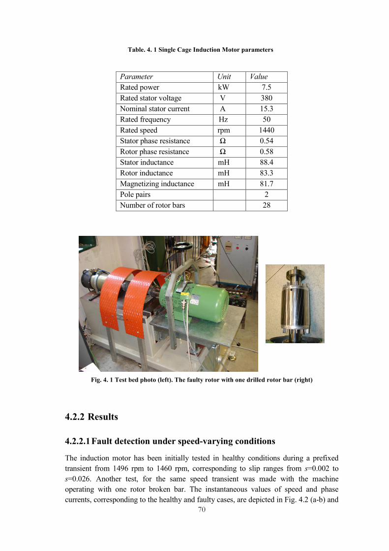
70

Table. 4. 1 Single Cage Induction Motor parameters

Parameter Unit Value

Rated power kW 7.5

Rated stator voltage V 380

Nominal stator current A 15.3



Stator phase resistance Ω 0.54

Rotor phase resistance Ω 0.58

Stator inductance mH 88.4

Rotor inductance mH 83.3

Magnetizing inductance mH 81.7

Pole pairs 2

Number of rotor bars 28

Fig. 4. 1 Test bed photo (left). The faulty rotor with one drilled rotor bar (right)

4.2.2 Results

4.2.2.1 Fault detection under speed-varying conditions

The induction motor has been initially tested in healthy conditions during a prefixed

transient from 1496 rpm to 1460 rpm, corresponding to slip ranges from s=0.002 to

s=0.026. Another test, for the same speed transient was made with the machine

operating with one rotor broken bar. The instantaneous values of speed and phase

currents, corresponding to the healthy and faulty cases, are depicted in Fig. 4.2 (a-b) and

71

Fig. 4.2 (c-d) respectively. For the considered speed range, approximation a9 was chosen

for extracting the contribution of the fault components (1-2s)f and (1+2s)f .Therefore the

choice of fsl is made to shift these fault components inside the frequency interval [0,

3.125] Hz corresponding to approximation. For the sake of clarity only the a9 signal will

be reported. In healthy condition, the 9th approximation signal a9, resulting from the

wavelet decomposition of the stator phase current, does not show any kind of variation

(Fig. 4.3). This indicates the absence of the fault component (1-2s)f, leading to diagnose

the healthy condition of the motor under speed-varying condition.

Fig. 4. 2 Instantaneous values of a-b) speed and c-d) stator phase currents under healthy and one

rotor broken bar respectively

However, in faulty condition (one rotor broken bar) approximation a9 shows significant

variation in magnitude observed in Fig. 4.4. During the first time period (t=0s to t=2s),

under a constant speed of 1496 rpm, the 9th approximation signal, representative of the

(1-2s)f frequency component, do not show any important variations. This is due to the

fact that at low load level (under 4% of the nominal torque) the fault frequencies are

practically superimposed to the fundamental and magnitudes are not detectable. During

deceleration (around t=2s), a9 shows particular magnitude escalation proportional to the

abrupt deceleration until reaching a quasi steady-state magnitude (under 66% of the

nominal torque).

0 2 4 6 8 101450

1460

1470

1480

1490

1500

1510- a -

Time (s)

Sp

eed

(rp

m)

0 2 4 6 8 101450

1460

1470

1480

1490

1500

1510- b -

Time (s)

Sp

eed

(rp

m)

0 2 4 6 8 10

-20

-10

0

10

20

- c -

Time (s)

Cu

rre

nt

(A)

0 2 4 6 8 10

-20

-10

0

10

20

- d -

Time (s)

Cu

rre

nt

(A)

72

More in detail, the oscillations observed in the signal a9, with quasi-constant amplitude,

follow a characteristic pattern that fits the evolution in frequency of the fault component

(1-2s)f, during the speed transient.

The second rotor fault signature tracked is related to the fault component at frequency

(1+2s)f. The corresponding experimental results, under healthy and rotor broken bar are

presented in Fig. 4.5 and Fig. 4.6. The same observations as for the signature of the side

band (1-2s)f under the considered rotor unbalance, are reached; the comparison of the

approximation signal a9, issued from wavelet decomposition of the stator phase current,

under healthy (Fig. 4.5-b) and rotor broken bar (Fig. 4.6-b) reproduce clearly the

magnitude evolution of the fault component (1+2s)f dynamically over time.

If we confine our attention on the approximation signal a9 depicted in Fig. 4.4-b and Fig.

4.6-b, we can notice that the rotor fault signature issued from the fault component (1-2s)f

is more relevant than the corresponding one related to the (1+2s)f component. This is

mainly due to the the machine-load inertia effect on high order rotor fault harmonics.

The 9th approximation signal obtained from the experimental results shows the

sensitivity and the effectiveness of this particular signal a9 to reproduce the contribution

of the frequency components (1-2s)f and (1+2s)f under large speed varying conditions.

Fig. 4. 3 DWT analysis of stator phase current under speed-varying condition, for tracking the

fault component (1-2s)f ; Healthy condition

0 1 2 3 4 5 6 7 8 9 10

-20

-10

0

10

20

- a -

Time (s)

Cu

rre

nt

(A)

0 1 2 3 4 5 6 7 8 9 10-1.2

-0.8

-0.4

0

0.4

0.8

1.2- b -

Time (s)

a9

73


fault component (1-2s)f ; One Broken Bar


fault component (1+2s)f ; Healthy condition

0 1 2 3 4 5 6 7 8 9 10

-20

-10

0

10

20

- a -

Time (s)

Cu

rren

t (A

)

0 1 2 3 4 5 6 7 8 9 10-1.2

-0.8

-0.4

0

0.4

0.8

1.2- b -

Time (s)

a9

0 1 2 3 4 5 6 7 8 9 10

-20

-10

0

10

20

- a -

Time (s)

Cu

rren

t (A

)

0 1 2 3 4 5 6 7 8 9 10-1.2

-0.8

-0.4

0

0.4

0.8

1.2- b -

Time (s)

a9

74


fault component (1+2s)f ; One Broken Bar

4.2.2.2 Fault quantification

Once the machine is qualitatively diagnosed, the fault indicator based on a cyclic mean

power calculation of the approximation a9, resulting from the wavelet decomposition

applied to one stator current, has been processed to evaluate quantitatively the degree

of the fault extent.

The cyclic evolution of the fault indicator mPa9, representative of the contributions of

the fault components components (1-2s)f and (1+2s)f , issued from the experimental

tests (Figs. 4.3-4.6), under healthy and rotor broken bar conditions are depicted in Fig.

4.7 and Fig. 4.8 respectively. In healthy condition, and under large range of speed

variations, mPa9 does not show any significant change. Consequently, the indicator

values for the healthy motor are considered as a baseline to set the threshold for

discriminating healthy from faulty conditions. Under rotor broken bar condition the

calculated mPa9 indicator shows a noteworthy increase. The large energy deviation

observed in faulty condition proves the effectiveness of the proposed approach, since

the transient speed motor operation does not disturb the fault assessment, in

comparison with the healthy case.

0 1 2 3 4 5 6 7 8 9 10

-20

-10

0

10

20

- a -

Time (s)

Cu

rre

nt (A

)

0 1 2 3 4 5 6 7 8 9 10-1.2

-0.8

-0.4

0

0.4

0.8

1.2- b -

Time (s)

a9

75

Fig. 4. 7 Cyclic values of the fault indicator mPa9, resulting from the 9th wavelet decomposition level

of the signals Isl under healthy and rotor bar broken (red and blue) during the tracking of (1-2s)f

component

Fig. 4. 8 Cyclic values of the fault indicator mPa9, resulting from the 9th wavelet decomposition level

of the signals Isl under healthy and rotor bar broken (red and blue) during the tracking of (1+2s)f

component

0 10 20 30 40 50 60 70 800

0.05

0.1

0.15

0.2

0.25

0.3

0.35

0.4

0.45

0.5

TIN

mP

a9

Healthy Broken bar

0 10 20 30 40 50 60 70 800

0.05

0.1

0.125

TIN

mP

a9

Healthy Broken bar

76

4.3 Analysis of rotor fault in double cage induction machine

Successful detection of outer cage faults in DCIMs requires understanding

similarities and differences with single cage broken bars phenomenon. The main

similarity between these two classes of motors in case of rotor fault is the existence of

interbar currents [1]-[5], and the chain of fault harmonics that appears in stator line-

currents [6]-[8].

For large or double squirrel cage motors, as long as the contact impedance between

the rotor bars and iron core is small or the copper bars are directly inserted into the

laminated iron slots, the broken bars are no longer a physical condition ensuring an open

circuit, since inter-bar or cross path currents can flow. If the resistance between the bars

and the iron core is low, currents will start to flow between the bars through the

lamination, which increases the stray-load losses in the machine and affect the torque

during the start-up [3]-[4]. Subsequently, these currents interact with the radial

component of the air-gap magnetic field, and compensate the rotor asymmetry caused

by rotor bar breakage and leads to axial vibrations [1],[4] and to temperature increase

[9]. In DCIMs these interactions can reduce significantly the amplitudes of rotor fault

components.

Another typical behavior of induction motors with rotor broken bars is the existence of

sideband components in the line currents at frequencies (12s)f whose amplitudes are

usually monitored for rotor diagnostic. The main difference between DCIMs and single

cage motors in case of broken bars is related to the inherent structure of the double cages

[10]. Double cage motors have two squirrel cages shorted with a common end ring or

with separate end rings. The schematic and the electrical equivalent circuit of the double

cage rotor are shown in Fig. 4.9. The outer cage is usually composed of small high

resistivity material bars, while the inner cage is made of larger, low-resistance bars [11].

The iron between the outer cage and the inner cage, together with the proximity of the

outer cage with the stator windings, causes the outer cage leakage reactance to be low.

Conversely, the leakage inductance of the inner cage is large since the magnetic

reluctance of flux path closing through the inner bar is low (Fig. 4.9).

Therefore, the rotor current is mainly confined to the high resistance outer cage at high

slip (i.e., startup) due to the dominance of the leakage inductance, thus obtaining high

startup torque. When steady state operation is reached, the leakage inductance is

negligible (low slip) and the outer cage resistance is dominant, which causes the current

to flow mainly in the low resistance inner cage. The rotor operates as a normal low-

resistance rotor, and the sensitivity of detecting the rotor fault from stator current is

significantly reduced. Considering that the depth of flux penetration into the rotor is

inversely proportional to the square root of the rotor frequency, the inner cage can be

nearly disregarded during the startup or during any abrupt slip increase due to load

transients.

77

Fig. 4. 9 Electrical equivalent circuit representation of a double squirrel cage induction motor

The sensitivity of MCSA has been experimentally evaluated in [7], [12] for single cage

and double cage rotor machines. It can be seen in Fig. 4.10 that the sensitivity of MCSA

for outer cage damage in double cage rotors under rated load is significantly lower than

that of the single cage rotor under identical conditions. The fl component is relatively

lower by 18 ~ 22dB for the double cage design, which corresponds to a decrease in

sensitivity by a factor of 10. The situation is worse for time-varying loads since the fault

components spread out resulting in lower peak magnitude. Considering that the default

fault alarm level for broken bars is set at -45~-35dB in commercial MCSA products (to

avoid false alarms) [12]-[13], outer cage faults of double cage motors are unlikely to be

detected unless a method dedicated to double cage motors is used.

Fig. 4. 10 Experimental measurements of broken bar component, frffc, with on-line MCSA under rated load for 0-3/44 broken bars for (left) single cage deep bar Al die cast rotor; (right) double cage

fabricated brass-Cu separate end ring rotor [7]

78

4.3.1 Motor Current Signature Analysis

4.3.1.1 System description

Experimental verification of the proposed method was performed on a 380V, 7.5 Hp,

12 A induction motor with a custom-made double cage rotor. A fabricated copper

separate end ring double cage rotor, shown in Fig. 4.11, was constructed to fit the stator

of an aluminum die cast induction motor, already available. The outer cage was made of

brass, which is common in large motors for obtaining high starting torque. The custom-

made rotor is designed and built so that it allows testing of the proposed method on a

motor representative of large motors.

The tests were performed for the healthy rotor and a faulty rotor after cutting 3 of 44

rotor bars at the bar end ring joint. The MCSA results shown for the double cage rotor in

Fig. 4.10 are obtained with the same test rotor. The motor load was controlled by

adjusting the field voltage of a 30 Hp DC generator coupled to the motor. Commercial

current sensors and a 16 bit DAQ board were used to measure the stator-line current isa

(the sampling frequency fs was 960 Hz) over a data acquisition window of 10 seconds

under load transient conditions from 10% to 90% of the full load. The second series of

tests was carried out during an acquisition time interval of 25 seconds under a load

profile from 10% to 50% then to 90% of the full load.

(a) (b)

Fig. 4. 11 Custom designed fabricated copper separate end ring double cage rotor sample with brass outer cage and copper inner cage(a), and the corresponding rotor lamination (b)

4.3.1.2 Results

4.3.1.2.1 Rotor Fault detection

A six level decomposition (n=6) was chosen to cover the frequency bands of the fault

79

components, as shown in Table 4.2. The proposed diagnosis approach was applied to the

stator current with lslf =52.10 Hz and then with r

slf =60.39 Hz, to isolate the contribution

of the fault components fl and fr, respectively. The first series of tests were conducted

under a large speed transient during 10 seconds, as reported by the speed profiles in

Figs. 4.12-a and 4.13-a, for healthy rotor and for three rotor outer cage broken bars,

respectively. The corresponding stator currents are shown in Figs. 4.12-b and 4.13-b.

The sixth-level approximation signals resulting from the DWT of )(ti lsl in healthy and

faulty conditions, computed under the assumption of a sliding frequency lslf =52.10Hz,

are depicted in Figs. 4.12-c and 4.13-c respectively.

Table. 4. 2 Frequency bands of approximation and detail signals

Approximation

signal, aj

Frequency

bands (Hz) Detail Signal, dj

Frequency

bands (Hz)

a6 [0 – 7.5] d6 [7.5 – 15]

a5 [0 – 15] d5 [15 – 30]

a4 [0 – 30] d4 [30 – 60]

In healthy condition, it can be observed that the approximation signal a6 (Fig. 4.12-c)

does not show any variation. This fact indicates that the fault component fl is absent in

the stator current (Fig. 4.12-b), which leads to the diagnosis of “healthy” condition of

the DCIM.

On the contrary, a significant variation in the amplitude of the approximation signal a6

can be observed under a fault condition with three broken outer cage bars, as shown in

Fig. 4.13-c. In steady state, under light load conditions (10% rated load), important

variations in la6 cannot be observed between 0~4 s. This is due to the fact that fault

components with small magnitude, superimposed on the fundamental, are not detectable

under light load conditions. However, during the deceleration transient due to the load

variation around t≈4s, an escalation in the magnitude of la6 proportional to the rate of

deceleration can be observed, as shown in Fig. 4.13-c.

The increase in the 6th approximation signal can be observed until reaching a quasi

steady-state magnitude at 90% rated load. The oscillations observed in the signal la6

with quasi-constant amplitude are the consequence of the time evolution of the

component fl issued from the stator current (Fig. 4.13-b) during the speed transient.

The second rotor fault signature tracked is related to the right sideband component at

frequency fr.

The corresponding experimental results, under healthy and three broken outer cage bars

are presented in Figs. 4.12-d and 4.13-d, respectively.

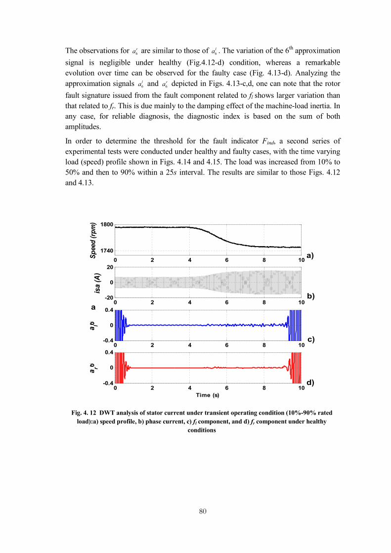
80

The observations for ra6 are similar to those of la6 . The variation of the 6th approximation

signal is negligible under healthy (Fig.4.12-d) condition, whereas a remarkable

evolution over time can be observed for the faulty case (Fig. 4.13-d). Analyzing the

approximation signals la6 and ra6 depicted in Figs. 4.13-c,d, one can note that the rotor

fault signature issued from the fault component related to fl shows larger variation than

that related to fr. This is due mainly to the damping effect of the machine-load inertia. In

any case, for reliable diagnosis, the diagnostic index is based on the sum of both

amplitudes.

In order to determine the threshold for the fault indicator Find, a second series of

experimental tests were conducted under healthy and faulty cases, with the time varying

load (speed) profile shown in Figs. 4.14 and 4.15. The load was increased from 10% to

50% and then to 90% within a 25s interval. The results are similar to those Figs. 4.12

and 4.13.

Fig. 4. 12 DWT analysis of stator current under transient operating condition (10%-90% rated

load):a) speed profile, b) phase current, c) fl component, and d) fr component under healthy

conditions

0 2 4 6 8 10

1740

1800

Sp

eed

(rp

m)

a0 2 4 6 8 10

-20

0

20

isa (

A)

0 2 4 6 8 10-0.4

0

0.4

al6

0 2 4 6 8 10-0.4

0

0.4

Time (s)

ar6

a)

b)

c)

d)

81

Fig. 4. 13 DWT analysis of stator current under transient operating condition (10%-90% rated

load):a) speed profile, b) phase current, c) fl component, and d) fr componentwith3 broken outer

cage bars

Fig. 4. 14 DWT analysis of stator current under transient operating condition (10%-50%-90%

rated load): a) speed profile, b) phase current, c) fl component, and d) fr component under

healthy conditions

0 2 4 6 8 10

1740

1800

Sp

eed

(rp

m)

a0 2 4 6 8 10

-20

0

20is

a (

A)

0 2 4 6 8 10-0.4

0

0.4

al6

0 2 4 6 8 10-0.4

0

0.4

Time (s)

ar6

a)

b)

c)

d)

0 5 10 15 20 25

1740

1800

Sp

eed

(rp

m)

a)

d)

b

b)

c)

0 5 10 15 20 25-20

0

20

isa

(A

)

0 5 10 15 20 25-0.4

0

0.4

al6

0 5 10 15 20 25-0.4

0

0.4

Time (s)

ar6

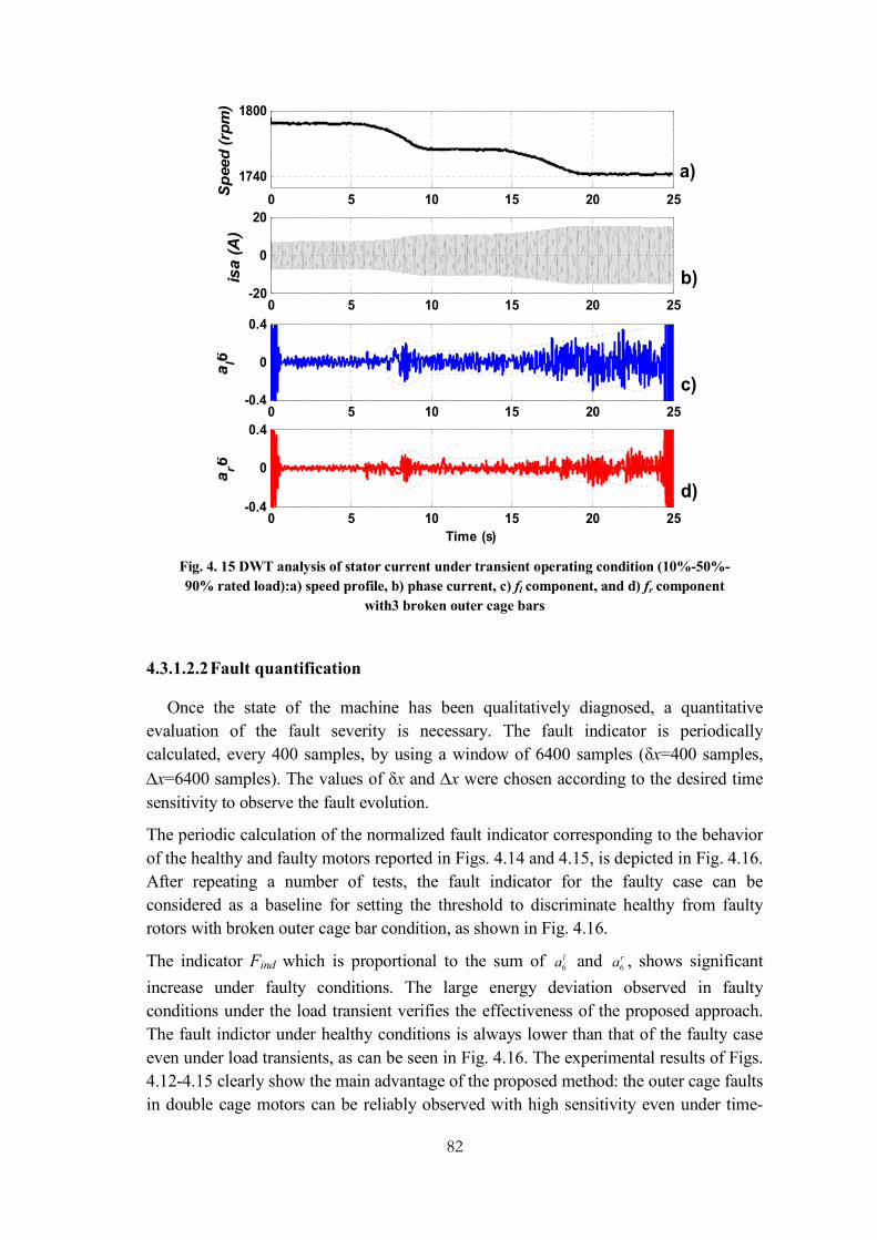
82

Fig. 4. 15 DWT analysis of stator current under transient operating condition (10%-50%-

90% rated load):a) speed profile, b) phase current, c) fl component, and d) fr component

with3 broken outer cage bars

4.3.1.2.2 Fault quantification

Once the state of the machine has been qualitatively diagnosed, a quantitative

evaluation of the fault severity is necessary. The fault indicator is periodically

calculated, every 400 samples, by using a window of 6400 samples (δx=400 samples,

x=6400 samples). The values of δx and x were chosen according to the desired time

sensitivity to observe the fault evolution.

The periodic calculation of the normalized fault indicator corresponding to the behavior

of the healthy and faulty motors reported in Figs. 4.14 and 4.15, is depicted in Fig. 4.16.

After repeating a number of tests, the fault indicator for the faulty case can be

considered as a baseline for setting the threshold to discriminate healthy from faulty

rotors with broken outer cage bar condition, as shown in Fig. 4.16.

The indicator Find which is proportional to the sum of la6 and ra6 , shows significant

increase under faulty conditions. The large energy deviation observed in faulty

conditions under the load transient verifies the effectiveness of the proposed approach.

The fault indictor under healthy conditions is always lower than that of the faulty case

even under load transients, as can be seen in Fig. 4.16. The experimental results of Figs.

4.12-4.15 clearly show the main advantage of the proposed method: the outer cage faults

in double cage motors can be reliably observed with high sensitivity even under time-

0 5 10 15 20 25

1740

1800

Sp

eed

(rp

m)

a)

d)

b

b)

c)

0 5 10 15 20 25-20

0

20is

a (

A)

0 5 10 15 20 25-0.4

0

0.4

al6

0 5 10 15 20 25-0.4

0

0.4

Time (s)

ar6

83

varying load transients as the assessment is not disturbed for a healthy machine under

load transients.

Fig. 4. 16 Values of the fault indicators: normalized Find (Black line)resulting from the 6th

wavelet decomposition level of the stator current under healthy and faulty (3 broken outer

cage bars) conditions with speed-varying conditions. Left side component (Blue line), and

right side component (Red line)

4.3.2 Motor Vibration Signature Analysis

In healthy conditions only the fundamental frequency f exists in stator currents of a

double cage induction machine. If the rotor part is damaged, the rotor symmetry of the

machine is lost producing a reverse rotating magnetic field related to an inverse

sequence component at frequency −sf. This inverse sequence is reflected on the stator

side, producing the frequency (1−2s)f. These frequency components generate

electromagnetic and mechanical interactions between stator and rotor parts.

Consequently torque and speed ripple effects are generated at frequency 2sf, which

modulate the rotating magnetic flux [6].

This modulation produces two current components, i.e., an additional left-side

component at (1−2s)f and a right side component at (1+2s)f. Following this interaction

process, the frequency content of the stator currents show series of fault components at

the following frequencies ((1±2ks)f)k=1,2,3,…). More specifically, for large or double

squirrel-cage motors, as long as the contact impedance between the rotor bars and iron

core is small or the copper bars are directly inserted into the laminated iron slots, the

broken bar is no longer a physical condition ensuring an open circuit and inter bar or

cross-path currents can flow. As a consequence, these inter bar transverse currents

interact with the radial stator flux density, generating axial forces. These facts lead

mainly to the presence of a first chain of fault frequency components at

(fmec±2ksf)k=1,2,3,…, and a second one at ((6-2ks)f)k=1,2,3,…, in radial and axial vibration

0 10 20 30 40 50 6010

-4

10-3

10-2

10-1

100

101

TIN

[%]

mPa6l (3outer cage BRB)

mPa6r (healthy)

mPa6r (3outer cage BRB)

mPa6l (healthy)

Find

(healthy)

Find

(3outer cage BRB)Threshold for 3outer cage BRB detection

84

directions (fmec denotes the mechanical speed of the motor) [15]- [18]. In the following,

the focus will be exclusively on tracking the most relevant fault components of the

harmonic chains((6-2ks)f)k=1,2,3,… and (fmec±2ksf)k=1,2,3,…, issued from axial vibrations.

4.3.2.1 System description

In order to evaluate the performances of the proposed approach, two double cage

induction motors are available; one healthy, and the second with a drilled broken bar

(the bar was completely disconnected from the common end-ring). The characteristics of

the double cage induction motors used for experiments are presented in Table 4.3. A

three-phase autotransformer of 30 kVA, 0-380 V is used as motor regulated supply. A

four quadrants 7,83 kW dc electrical drive is adopted to reach the different planned load

conditions. One piezoelectric accelerometers Brüel & Kjær model 4507 B 005, was

mounted for measuring axial vibrations of the core motors. Fig. 4.17 shows detailed

photos of the healthy and drilled rotor (left), and details of the test-bed (right). In Fig.

4.18 and Fig. 4.19 instantaneous values of rotor speed and axial vibration signals are

depicted for healthy and faulty conditions respectively. All signals reported have been

recorded during 20 seconds. The tests were carried out considering a speed transient

from 0% to 70% of full load.

Table. 4. 3 Data of the double rotor cage motor

Data Value

Rated Power kW 5.5

Rated stator voltage V 400

Rated current A 13



Rotor diameter mm 110

Axial length of the rotor mm 90

Air gap length mm 0.5

Number of stator slots 36

Number of rotor slots 30

Fig. 4. 17 Photos of the healthy and drilled broken bar (left), and details of the test-bed (right)

85

Fig. 4. 18 Instantaneous values of speed (a), and axial vibration signal (b) under healthy

conditions

Fig. 4. 19 Instantaneous values of speed (a), and axial vibration signal (b) under broken bar

4.3.2.2 Results

4.3.2.2.1 Rotor Fault detection

With a sampling frequency fs=2.0kHz, a six level decomposition (J=6) was chosen in

order to cover the frequency bands in which we can track the contribution of the first

chain of harmonic ((6-2ks)f)k=1,2,3,…. The second chain of fault component

0 2 4 6 8 10 12 14 16 18 202850

2900

2950

3000

3050- a -

Time (s)

Sp

eed

(rp

m)

0 2 4 6 8 10 12 14 16 18 20-1

-0.5

0

0.5

1- b -

Time (s)

Accele

rati

on

(m

/s2)

0 2 4 6 8 10 12 14 16 18 202850

2900

2950

3000

3050- a -

Time (s)

Sp

ee

d (

rp

m)

0 2 4 6 8 10 12 14 16 18 20-1

-0.5

0

0.5

1- b -

Time (s)

Accele

rati

on

(m

/s2)

86

(fmec±2ksf)k=1,2,3,…, will be tracked in a frequency band corresponding to seven level

decomposition (J=6). The frequency band repartition corresponding to the above

decompositions are detailed in Table. 4.4. The chains of fault components ((6-

2ks)f)k=1,2,3,… and (fmec±2ksf)k=1,2,3,…, will be tracked in the frequency bands [0: 15.625]

and [0: 7.812] respectively, after appropriate frequency sliding applied to axial vibration

signals. All signals reported have been recorded during 10 seconds.

Table. 4. 4 Frequency bands at each level of decomposition

Approximations «aj »

Frequency bands (Hz)

Details « dj »

Frequency bands (Hz)

a7 : [0 – 7.812] d7 : [7.812 – 15.625] a6 : [0 – 15.625] d6 : [15.625 – 31.25] a5 : [0 – 31.25] d5 : [31.25 – 62.5] a4 : [0 – 62.5] d4 : [62.5 – 125] a3 : [0 – 125] d3 : [125 – 250] a2 : [0 – 250] d2 : [250 – 500] a1 : [0 – 500] d1 : [500 – 1000]

The wavelet decompositions of the axial vibration signals (vax) in healthy condition, for

each chain or rotor fault components, are used as references in comparison to the faulty

cases.

During the considered transient conditions, the investigated axial vibration signals under

healthy and one drilled broken bar are depicted in Figs. (4.20-a, 4.22-a) and Figs. (4.21-

a, 4.24-a) respectively. After a frequency sliding of 286.16 Hz applied to the axial

vibration signals vax under healthy and one rotor broken bar condition, the resulting

signals Vsl were analysed by DWT thereby. The corresponding Wavelet Analysis results

(a6), under healthy and faulty conditions are reported in Fig. 4.20-b and Fig.4.21-b

respectively.

In healthy condition, the approximation signal of interest (a6), depicted in Figure 4.20-b,

shows very low variations. This indicates the absence of the chain of rotor fault

component ((6-2ks)f)k=1,2,3,… , leading to diagnose the healthy condition of the motor

under speed-varying conditions. Under faulty condition, the contribution of the chain of

fault components ((6-2ks)f)k=1,2,3,… , observed on the 6th approximation signal, is very

relevant in comparison to the healthy case (Fig. 4.21-b). More in detail, the oscillations

observed in the signal a6, with quasi-constant amplitude, follow a characteristic pattern

that fits the evolution in frequency of the considered chain of fault components. The

same observations are valuable for the contribution of the chain of rotor fault component

(fmec±2ksf)k=1,2,3,…, observed under healthy and faulty conditions, in Fig. 4.22-b and Fig.

4.24-b respectively. The variations observed in the approximation signal a7 are evident

in faulty case (Fig. 4.22-b) in comparison to the healthy one (Fig. 4.24-b), leading to a

87

clear discrimination between healthy and faulty conditions, through the evolution of the

wavelet signal a7.

Fig. 4. 20 Instantaneous values of axial vibration signal (a), and its corresponding Wavelet

analysis (b) under healthy condition


analysis (b) under rotor broken bar.

0 2 4 6 8 10 12 14 16 18 20-1.5

-1

-0.5

0

0.5

1

1.5- a -

Time (s)

Acc

ele

rati

on

(m

/s2

)

0 2 4 6 8 10 12 14 16 18 20-0.05

0

0.05- b -

Time (s)

a6

0 2 4 6 8 10 12 14 16 18 20-1.5

-1

-0.5

0

0.5

1

1.5- a -

Time (s)

Ac

ce

lera

tio

n (

m/s

2)

0 2 4 6 8 10 12 14 16 18 20-0.05

0

0.05- b -

Time (s)

a6

88


analysis (b) under healthy condition


analysis (b) under rotor broken bar.

0 2 4 6 8 10 12 14 16 18 20-1.5

-1

-0.5

0

0.5

1

1.5- a -

Time (s)

Acce

lera

tio

n (m

/s2)

0 2 4 6 8 10 12 14 16 18 20-0.05

0

0.05- b -

Time (s)

a7

0 2 4 6 8 10 12 14 16 18 20-1.5

-1

-0.5

0

0.5

1

1.5- a -

Time (s)

Ac

ce

lera

tio

n (

m/s

2)

0 2 4 6 8 10 12 14 16 18 20-0.05

0

0.05- b -

Time (s)

a7

89

4.3.2.2.2 Fault quantification

After the above qualitative analysis of the fault, a quantitative evaluation of the fault

extend was conducted. The fault indicator is periodically calculated (every 400 samples)

using a window of 6400 samples, where δn=150 samples and Δn=6400 samples.

The mean power calculation results, issued from the approximation signal a6, which

have been obtained in Figs. 4.20-b and 4.21-b, are depicted in Fig. 4.24. In healthy

condition, the calculated mPa6 indicator don’t show any significant changes.

Consequently, the indicator values for the healthy motor response are considered as a

baseline to set the threshold for discriminating healthy from rotor broken bar conditions.

In faulty conditions the calculated mPa6 indicator shows significant increase. The large

energy deviation observed in faulty conditions reflect the presence of the chain of rotor

fault components ((6-2ks)f)k=1,2,3,…, leading to an effective diagnosis procedure for

broken bars in double squirrel cage induction machine.

The above conclusions are valid also for the quantification process related to the

contribution of the chain of rotor fault components (fmec±2ksf)k=1,2,3,…, and depicted in

Fig. 4.25 for the healthy and faulty cases. Other fault components could be treated in the

same way for improving the quantification process.

Fig. 4. 24 Cyclic values of the mPa6 fault indicator calculation issued from the approximation

signal a6, under healthy (Red) and rotor broken bar (Blue) conditions.

0 20 40 60 80 100 120 140 160 180 2000

1

2

3

4

5

6

7

8x 10

-4

TIN

mP

a6

90

Fig. 4. 25 Cyclic values of the mPa7 fault indicator calculation issued from the approximation

signal a7, under healthy (Red) and rotor broken bar (Blue) conditions.

4.4 Conclusion

In this chapter, the proposed diagnosis technique was validated for the detection of

rotor broken bars in squirrel cage induction motors. As first application, the proposed

diagnosis technique was successfully applied for rotor broken bars detection for single

cage induction machine, by investigating MCSA. The second part of this chapter is

focused on the detection of rotor outer cage bar faults for double cage motors. Using

the proposed diagnosis technique, motor current signature analysis and motor

vibration signature analysis were successfully applied to the detection of outer cage

faults, and for motors operating under time-varying conditions.

0 20 40 60 80 100 120 140 160 180 2000

1

2

x 10-4

TIN

mP

a7

91

REFERENCES

[1] R.F. Walliser and C. F. Landy, "Assessment of interbar currents in double cage

induction motors with broken bars," IEEE Trans. Energy Convers., vol. 9, no. 1,

pp. 159–164, Mar. 1994.

[2] R. Carlson, C.A. da Silva, N. Sadowski, Y. Lefevre, and M. Lajoie-Mazenc,

“Analysis of the Effect of Inter-Bar Currents on the Performance of Polyphase

Cage-Induction Motors, ” IEEE Trans. Ind. Appl., vol. 39, no. 6, pp. 1674–1680,

Nov./Dec. 2003.

[3] D.G. Dorrell , P.J. Hollik, C.B. Rasmussen, ”Analysis and Effects of Inter-Bar

Current and Skew on a Long Skewed-Rotor Induction Motor for Pump

Applications”, IEEE Trans. on Magn.,vol. 43, no. 6, pp. 2534-2536, 2007.

[4] D.G. Dorrell, T.J.E. Miller, C.B. Rasmussen, “Inter-bar currents in induction

machines”, IEEE Trans. Ind. Appl., vol. 39, no. 3, pp. 676–684, May/Jun. 2003.

[5] I. Kerszenbaum, C.F. Landy, “The existence of inter-bar currents in three phase

squirrel cage motors with rotor-bar and end-ring faults,” IEEE Trans. Pow.

Appar. and Syst., vol. PAS-103, no. 7, pp. 1854-1862, July 1984.

[6] A. Bellini, F. Filippetti, C. Tassoni, and G. A. Capolino, "Advances in diagnostic

techniques for induction machines", IEEE Trans. Ind. Electron., Vol.55, N° 12,

Dec. 2008.

[7] J. Park, B. Kim, J. Yang, K. Lee, S.B. Lee, E.J. Wiedenbrug, M. Teska, and S.

Han, " Evaluation of the detectability of broken rotor bars for double squirrel

cage rotor induction motors," Proc. of IEEE ECCE, pp. 2493-2500, Sept. 2010.

[8] J. A. Daviu, M. R. Guasp, J. P. Linares, J. Park, S.B. Lee, J. Yoo, C. Kral,

"Detecion of broken outer cage bars for double cage induction motors under the

startup transient", IEEE Trans. Ind. Appl., vol. 48, no. 5, pp. 1539–1548,

Sep./Oct. 2012.

[9] J. Mroz, “Temperature field distribution of a double squirrel-cage rotor during

startup,” IEE Proceedings – Electric Power Applications, vol. 152, no. 6, pp.

1531-1538, Nov. 2005.

[10] Motors and generators, NEMA standards pub. MG 1-2006, 2006.

[11] P.L. Alger, and J.H. Wray, “Double and triple squirrel cages for polyphase

induction motors,” AIEE Transactions Part III – Power Apparatus and Systems,

vol. 78, no.2, pp. 637-645, Jan. 1953.

[12] G.C. Stone, and I. Culbert, “The testing tools,” IEEE Industry Applications

Magazine, no. 14, vol. 6, pp. 48-53, Nov./Dec. 2008.

[13] EXP 4000 Users Manual, Baker Instrument Company – An SKF Group

Company, Fort Collins, CO, Feb. 2010.

92




Sep. 2011.

[15] G. H. Muller and C. F. Landy, "A novel method to detect broken rotor bars in

squirrel cage induction motors when interbar currents are present, " IEEE Trans.

on Energy Conversion, Vol. 18, N° 1, pp. 71-79, Mar. 2003.

[16] C. Concari, G. Franceschini, and C. Tassoni, " Differential Diagnosis Based on

Multivariable Monitoring to Assess Induction Machine Rotor Conditions", IEEE

Trans. on Ind. Electronics, Vol. 55, N° 12, Dec. 2008.

[17] J. J. Rangel-Magdaleno, R. J. Romero-Troncoso, R. A. Osornio-Rios, E. Cabal-

Yepez, and L. M. Contreras-Medina, "Novel Methodology for Online Half-

Broken-Bar Detection on Induction Motors", IEEE Trans. on Inst. and Meas.,

Vol. 58, N° 5, May. 2009.

[18] A. Sadoughi, M. Ebrahimi, M. Moalem, and S. Sadri, "Intelligent Diagnosis of

Broken Bars in Induction Motors Based on New Features in Vibration

Spectrum", The IEEE-SDEMPED’07, pp. 106-111. Sep. 2007.

94

CHAPTER 5 : FAULT DIAGNOSIS

EXTENSION FOR MULTIPHASE

ELECTRICAL MACHINES

5.1 Introduction ........................................................................................................................... 95 5.2 Characterization of Rotor Demagnetization in Five-Phase Surface–Mounted Permanent Magnet Generator .......................................................................................................... 95

5.2.1 System description ......................................................................................................... 95 5.2.2 Results ............................................................................................................................ 102 5.2.3 Fault quantification...................................................................................................... 104

5.3 Characterization of stator fault in seven-phase induction machine .......................... 104 5.3.1 System description ....................................................................................................... 105 5.3.2 Results ............................................................................................................................ 106

5.4 Conclusion ........................................................................................................................... 109

References ......................................................................................................................................... 110

95

5.1 Introduction

In this chapter, the proposed diagnosis technique is extended to faults detection in

Multiphase electrical machines. Multiphase Permanent-Magnet Generators are an

attractive alternative to induction machines for a variety of applications owing to their

reliability and dynamic performance, suited for emerging applications such as

automotive or traction systems. In this context, diagnosing the status of the rotor

magnets is crucial for improving the reliability of the generators. This Chapter is

firstly focused on the demagnetization of the rotor magnet trailing edges, due to large

stator currents, in five-phase surface-mounted permanent magnet synchronous

generators under Time-varying conditions. Consequently, the classical application of

Fourier analysis for processing the back-emf induced in the α-β planes fails as the fault

components intended to be monitored to assess the magnets status are spread in a

bandwidth proportional to the speed variation. In this context, the back-emf induced in

the α-β planes is analyzed by the proposed diagnosis technique for the detection of

rotor demagnetization in multiphase surface-mounted permanent magnet generator

under speed-varying conditions. The proposed methodology is validated by means of

two dimensional (2-D) Finite Element Analysis (FEA) and numerical simulations.

Moreover, a cyclic quantification of the fault extent over time was introduced for

accurate rotor fault detection.

The second subpart of this section investigates the behavior of multiphase induction

machines with an odd number of phases in investigated under the assumption that the

stator winding is unbalanced owing to a fault or an incipient damage. The analysis

leads to a method to assess the unbalance condition of the machine, based on the

calculation of the space vectors of the stator currents in the available α-β planes.

Experimental results for the analysis established in time and frequency domains show

interesting results to be extended to time-frequency domain.

5.2 Characterization of Rotor Demagnetization in Five-Phase

Surface–Mounted Permanent Magnet Generator


The numerical modeling of the used five-phase surface-mounted PMSG is developed for healthy and local magnet demagnetization conditions. Multiple space vector theory is considered to represent the five-phase system by two space vectors and a zero- sequence component as detailed in Appendix.2. Under the assumptions usually adopted for the analysis of ac machines, the magnetic field produced by the stator windings in the air gap can be expressed in a stator reference frame in terms of stator current space vectors in the following compact form:

96

3 7 9* *3 7 91 1 3 3 1

5,

2 3 7 9S S S Sj j j jS wS wS wS

S S e wS S S S S

N K K Kh t K i e i e i e i e

p

(5. 1)

where, NS is the number of series-connected conductors per phase, is the air gap

length, p the number of pairs of poles, e the real part operator, KwS the -th winding

coefficient, S a stationary angular coordinate in electrical radians whose origin is

aligned with the magnetic axis of phase 1, whereas 1Si and 3Si are the stator current

space vectors.

The symbol “*” identifies the complex conjugate quantities. Besides the fundamental

component, (5.1) takes into account the third, the seventh and the ninth spatial

harmonics, and is expressed in terms of the instantaneous values of the stator current

vectors. It is worth noting that the fifth spatial harmonic is null, since it can be

generated only by the zero-sequence component of the stator currents, which is zero

owing to the star connection of the windings.

With the usually adopted control strategy for PMSGs, the air gap distribution of the

stator MMF is maximum along the quadrature axis. In this way, one half of each

magnet is reverse magnetized. This can lead to a local demagnetization of the rotor

magnets, which is reproduced by simply removing part of the magnetic material from

the trailing edge.

The magnetic field produced by the rotor magnets in the air gap, in a rotor reference

frame, can be written as:

3 53 53 5

7 97 97 9

2,

1 1

3 5

1 1

7 9

R

R R

R R

j jjMR R e

j jj jj j

j jj jj j

Hh t e e e

e e e e e e

e e e e e e

(5. 2)

where, R is an angular coordinate in electrical radians in the rotor reference frame, -

2 is the pole arc of the surface-mounted permanent magnets, and identifies the

demagnetized portion of the magnets (Fig. 5.1).

By neglecting the slot opening effect, and assuming a unitary relative recoil

permeability of the magnets, the value of HM can be expressed as:

0

M RM

BH

, (5. 3)

where, M is the magnet thickness, and BR is the residual flux density of the magnet

material.

97

m

R

Stator

Rotor

Fig. 5. 1 Schematic draw of a pair of surface-mounted permanent magnets in

healthy and fault conditions

Besides the fundamental component, (5.2) takes into account the third, the fifth, the

seventh and the ninth spatial harmonics. Fig. 5.2 shows the amplitude variation of

every single spatial harmonic in the flux density distribution as a function of the pole

arc reduction in electrical radians for the considered machine (Table.5.1).

Table. 5. 1 Five-Phase PMSG Parameters (FEA)

Rated torque 12 Nm

Torque over current ratio 2.4 Nm/A

Rated speed 3000 rpm

Phase resistance 0.55 Ohm

Phase reactance (100 Hz) 4.5 Ohm

Pole number 4

Stator inner radius 40 mm

Stator outer radius 68 mm

Stack length 100 mm

Slot number 40

Slot opening width 1.8 mm

Slot opening depth 0.5 mm

Stator winding pitch 9/10

Radius of the rotor surface 36 mm

Magnet-arc to pole-pitch ratio 77.14 / 90

Magnet radial thickness 3 mm

Magnet remanence 1.3 T

Relative recoil permeability 1.13

Magnetization type Radial

98

The amplitudes are normalized by the amplitude of the fundamental. It is a matter of

fact that a reduction of the pole arc leads to a variation of the harmonic content in the

flux linkage, and thus in the back-emf. In the present work, and as it is detailed below,

the focus is exclusively on tracking the contribution of the ninth and seventh inverse

harmonics issued from the back-emf.

To evaluate the stator linkage fluxes, it is necessary to consider the contributions of

the air gap magnetic field and of the leakage fluxes. The air gap magnetic field

contribution can be derived by means of (5.1) and (5.2).

Fig. 5. 2 Harmonic amplitude variation in the flux density distribution as a function of the

magnet pole arc reduction in electrical radians

The contribution of the leakage fluxes can be easily described by introducing two

leakage inductances (the leakage inductances LSd1 and LSd3 for the - and -

planes, respectively).

In conclusion, the mathematical model of the surface-mounted PMSG, written in terms of multiple space vectors, can be written as follows:

00

SS

dv

dt

, (5. 4)

11 1

SS S S

dv R i

dt

, (5. 5)

33 3

SS S S

dv R i

dt

, (5. 6)

0 1 20.26170

0.2

0.4

0.6

0.8

1

Magnet pole arc reduction (rad)

No

rmalized

Harm

on

ic A

mp

litu

des

1st Harmonic

3rd Harmonic

5th Harmonic

7th Harmonic

9th Harmonic

Reduced pole arc

99

where the zero-sequence and the - and -space vectors of the linkage fluxes are given by

50 5

jS e M e , (5. 7)

91 1 1 1 9

j jS S S M ML i e e , (5. 8)

3 73 3 3 3 7

j jS S S M ML i e e . (5. 9)

In (5.7)-(5.9), is the rotor position in electrical radians, whereas LS1 and LS3 are the

- and -synchronous inductances, which can be expressed as

22 9

1 1 181

wSS Sd SS wS

KL L L K

, (5. 10)

2 23 7

3 39 49wS wS

S Sd SS

K KL L L

, (5. 11)

where

20

2

5

2S

SS

L NL

p

, (5. 12)

and is the pole pitch.

The space vectors of the fluxes linked with the stator windings due to the permanent

magnet field harmonics, can be expressed as follows:

1 1

j jm M wSK e e (5. 13)

3 333

9

j jwSm M

Ke e

(5. 14)

7 777

49

j jwSm M

Ke e

(5. 15)

9 999

81

j jwSm M

Ke e

(5. 16)

where

02

2 S MM

L N H

(5. 17)

The electromagnetic torque Tem assumes the following form:

,1 ,3 ,7 ,9em em em em emT T T T T (5. 18)

where

100

,1 1 1

5

2

j j jem wS M ST p K i j e e e

(5. 19)

3 3 33,3 3

5

2 3

j j jwSem M S

KT p i j e e e

(5. 20)

7* 7 77,7 3

5

2 7

j j jwSem M S

KT p i j e e e

(5. 21)

9* 9 99,9 1

5

2 9

j j jwSem M S

KT p i j e e e

(5. 22)

As can be seen, four torque contributions are present, each one identified by the order

of the related spatial harmonic in the air gap.

Contributions Tem,1 and Tem,3 can be ripple free owing to the synchronization of 1Si with je , and 3Si with 3je . On the contrary, contributions Tem,7 and Tem,9 are oscillating,

because *3Si is not synchronized with 7je , as well as *

1Si is not synchronized with 9je .

Note that the stator current space vector 3Si is usually kept equal to zero by the control

system in a standard five-phase drive. A non-zero value of 3Si is used only in high

torque density motor drives, as discussed in [1]-[4]. In the present investigation, a null

value of 3Si is assumed. Consequently, only the contribution Tem,9 has to be minimized

in order to reduce the torque ripple. This goal can be obtained either by an opportune

choice of the permanent magnet pole arc or by suitable short-pitch stator windings.

Taking into account (5.5), (5.6), (5.8), (5.9), (5.13), (5.14), (5.16) and (5.17), the space

vectors 1Se and 3Se of the back-emf, can be expressed as shown in (5.23) and (5.24),

which emphasize the low order harmonic content of the back-emf space vectors.

21 1

999 2

2 cos2

2 9cos 9

9 2

jj

S M wS

jjM wS

e j K e e

j Ke e

(5. 23)

333 2

3

777 2

2 3cos 3

3 2

2 7cos 7

7 2

jjM wS

S

jjM wS

j Ke e e

j Ke e

(5. 24)

In order to validate the theoretical analysis of the emf harmonic content under speed

varying-conditions, the simulation of a five-phase surface-mounted PMSG has been

carried out using FEA. The parameters of the generator are summarized in Table 5.1.

A double-layer stator winding, having two slots per pole and per phase, with 9/10 coil

pitch, is considered (KwS9 = 0.024). The pole arc for the surface-mounted permanent

magnet has been reduced of one seventh in respect to the polar pitch in order to

eliminate the seventh harmonic in the resulting emf. The cross-section of the five-

phase PMSG, with a superimposed flux plot obtained by FEA, in healthy no-load

101

conditions, is shown in Fig. 5.3.

The simulations have been performed in no-load conditions under speed varying

conditions (from 1500rpm to 3000rpm), firstly with healthy magnets ( = 0°) and,

then, with magnets having a reduced pole arc ( = 15°) in order to reproduce a

demagnetization on the trailing edges. By means of the FEA simulations, the linkage

fluxes with the five stator phases have been determined as function of the rotor

position. For the analysis of the sensitivity to the fault, the emfs have been divided by

the rotor speed (expressed in electrical radians) obtaining the so called ‘normalized

emf’.

Fig. 5. 3 Cross-section of the five-phase PMSG, with a superimposed flux plot obtained by FEA,

in healthy no-load conditions.

The large speed transient profile adopted during the simulations under healthy and faulty

conditions is depicted in Fig. 5.4-a. The corresponding back-emfs under faulty

conditions are depicted in Fig. 5.4-b. All signals reported have been recorded during 15

seconds, with a sampling frequency of 3.2 kHz.

102

Fig. 5. 4 Instantaneous values of the electrical speed (a), and the corresponding back-emfs under

faulty conditions

5.2.1.1 Results

With reference to the machine whose parameters are reported in Table 5.1, the

sampling frequency fs is chosen equal to 3.2kHz and a three-level decomposition (J=3)

is adopted to cover the frequency bands in which the frequency component

characteristics of the fault can be tracked (see Table 5.2).

As explained in Section III, the contribution of 7th inverse harmonic component of the

normalized back-emf space vector /3Se can be observed in the approximation signal a3

after appropriate sliding frequency. In order to isolate the contribution of the 7th inverse

harmonic fault component in the frequency band of the approximation signal a3, a

sliding frequency fsl = -(7fS+12.5 Hz) was chosen to shift the α3-β3 components of the

normalized back-emfs under healthy and faulty conditions. As already explained, the

sliding frequency is chosen in such a way that the expected fault harmonic is shifted in

the middle of the frequency band of the approximation signal a3. The results of this

analysis are shown in Figs. 5.5-5.6. The wavelet decomposition obtained when the

machine is healthy should be compared with the one obtained in the case of faulty rotor.

The absence of amplitude variations in a3 (Fig. 5.5-b) is due to the low contribution of

the 7th harmonic in healthy conditions, which allows one to diagnose the healthy state of

the machine. By contrast, under a local demagnetization (Fig. 5.6-b) , it is possible to

notice an amplitude increase in the approximation signal a3, in comparison to the

healthy case (Fig. 5.5-b). This result means a clear detection of rotor demagnetization.

0 5 10 15

150

200

250

300

350

Time (s)

Ele

ctr

ical sp

eed

(ra

d/s

)

0 5 10 15-100

-50

0

50

100

Time (s)

[ V

. ]

back-emf1

back-emf2

back-emf3

back-emf4

back-emf5

10 10.005 10.01-100

-50

0

50

100

103

Table. 5. 2 Frequency band of each level

Approximations

«aj »

Frequency

bands (Hz)

Details

« dj »

Frequency

bands (Hz)

a3 : [0 – 200] d3 : [200 – 400]

a2 : [0 – 400] d2 : [400 – 800]

a1 : [0 – 800] d1 : [800– 1600]

Fig. 5. 5 Instantaneous values of the electrical speed (a), and the third approximation signal (a3)

issued from Wavelet analysis of the α3-β3 components of the back-emf space vector under healthy

conditions.

Fig. 5. 6 Instantaneous values of the electrical speed (a), and the third approximation signal (a3)

issued from Wavelet analysis of the α3-β3 components of the back-emf space vector under local

rotor magnet demagnetization conditions.

0 5 10 15

150

200

250

300

350

Time (s)

Ele

ctr

ica

l S

pe

ed

[ra

d/s

]

- a -

0 5 10 15

-5

0

5

Time (s)

a3

- b -

0 5 10 15

150

200

250

300

350

Time (s)

Ele

ctr

ical S

peed

[ra

d/s

]

- a -

0 5 10 15

-5

0

5

Time (s)

a3

- b -

104

5.2.1.2 Fault quantification

Once the state of the machine has been qualitatively diagnosed, a quantitative evaluation

of the fault severity is necessary. The fault indicator is periodically calculated, every 400

samples, by using a window of 6400 samples (δx=400 samples, x=6400 samples). The

values of δx and x were chosen according to the desired time sensitivity to observe the

fault evolution. Fig. 5.7 shows the shapes of the corresponding fault indicators in faulty

and healthy conditions respectively. These results mean that the proposed methodology

leads to a clear detection of rotor demagnetization.

Fig. 5. 7 Values of the fault indicator mPa3 (eS3), corresponding to the 7th inverse harmonic component, resulting from the approximation signal a3 under large speed transient, for healthy

and local rotor demagnetization (15°) conditions.

5.3 Characterization of stator fault in seven-phase induction

machine

Multiphase drives are receiving an increasing attention by the research community in high power applications. In this section, the behavior of seven-phase induction machine is investigated under incipient stator unbalance. The analysis leads to a method to assess the unbalance condition of the machine, based on the calculation of

the space vectors of the stator currents in the available - planes. The analytical model of a multiphase induction motor with unbalanced stator winding is completely developed in [5] . The investigation of the current stator space vectors in the available

- planes has shown interesting results for stator fault detection and localization. Results are confirmed by experimental tests.

0 20 40 60 80 100 1200

2

4

6

8

10

12

TIN

mP

a3

Demagnetized magnets (15°)

Healthy

105


Multiphase machines are usually fed by a multiphase inverter, whose command signals are calculated by a control system within a closed-loop scheme. Nevertheless it is of some interest to analyze the behavior of machine under the assumption that the control scheme is an open loop, such as the constant V/Hz control scheme. The main reason is that the understanding of such control schemes is the starting point for more complex cases.

A complete drive system has been built and some experimental tests have been realized. The experimental set-up consists of a 7-phase IGBT inverter and a 4 kW, 7-phase, 4-pole squirrel cage induction motor. The parameters of the motors are shown in Table 5.3. A schematic diagram and some pictures of the experimental set-up are shown in Fig. 5.8. The control algorithm is very simple, without any form of compensation of the voltage drop on the stator impedance.

All the tests have been carried out by feeding the motor with 80 V at 25 Hz. The resulting motor speed in healthy conditions is around 700 rpm, and the load has been adjusted so that the torque produced by the motor is 15 Nm, i.e., about two third of the rated torque.

During the experimental tests, an extern resistor has been added in series with the machine phases to reproduce a fault condition in a non-destructive way.

Table. 5. 3 Parameters of the Seven-Phase Machine

Trated = 24 Nm LS1 = 180 mH

Is,max = 7.5 A(peak) LR1 = 180 mH

IS1d,rated = 3.6 A(peak) M1 = 175 mH

frated = 50 Hz LS3 = 24 mH

RS = 1.3 LR3 = 24 mH

RR1 = 1.0 M3 = 19 mH

RR3 = 0.8 LS5 = 10 mH

RR5 = 0.6 LR5 = 10 mH

p = 2 M5 = 7mH

Laboratory controllable 3-ph

AC source (50 Hz) DC-link voltage

3-P Rectifier

…

7 Phases

7-P IM LOAD

…

Stator currents

(6 sensors)

7 PWM leg signals

Control system (DSP TI -TMS320F2812)

7-P Inverter dc-link

Additional resistance

Speed and torque sensors

a)

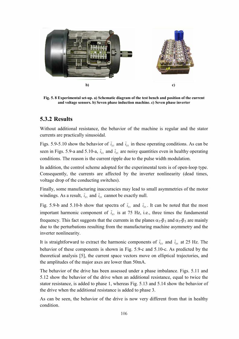
106

b) c)

Fig. 5. 8 Experimental set-up. a) Schematic diagram of the test bench and position of the current

and voltage sensors. b) Seven phase induction machine. c) Seven phase inverter

5.3.2 Results

Without additional resistance, the behavior of the machine is regular and the stator

currents are practically sinusoidal.

Figs. 5.9-5.10 show the behavior of 3Si and 5Si in these operating conditions. As can be

seen in Figs. 5.9-a and 5.10-a, 3Si and 5Si are noisy quantities even in healthy operating

conditions. The reason is the current ripple due to the pulse width modulation.

In addition, the control scheme adopted for the experimental tests is of open-loop type.

Consequently, the currents are affected by the inverter nonlinearity (dead times,

voltage drop of the conducting switches).

Finally, some manufacturing inaccuracies may lead to small asymmetries of the motor

windings. As a result, 3Si and 5Si cannot be exactly null.

Fig. 5.9-b and 5.10-b show that spectra of 3Si and 5Si . It can be noted that the most

important harmonic component of 3Si is at 75 Hz, i.e., three times the fundamental

frequency. This fact suggests that the currents in the planes 3-3 and 5-5 are mainly

due to the perturbations resulting from the manufacturing machine asymmetry and the

inverter nonlinearity.

It is straightforward to extract the harmonic components of 3Si and 5Si at 25 Hz. The

behavior of these components is shown in Fig. 5.9-c and 5.10-c. As predicted by the

theoretical analysis [5], the current space vectors move on elliptical trajectories, and

the amplitudes of the major axes are lower than 50mA.

The behavior of the drive has been assessed under a phase imbalance. Figs. 5.11 and

5.12 show the behavior of the drive when an additional resistance, equal to twice the

stator resistance, is added to phase 1, whereas Fig. 5.13 and 5.14 show the behavior of

the drive when the additional resistance is added to phase 3.

As can be seen, the behavior of the drive is now very different from that in healthy

condition.

107

The magnitudes of 3Si and 5Si are now sensibly greater and can be easily detected.

Their spectra confirm that the most important harmonic components are at 25 Hz, in

perfect agreement with the theoretical analysis.

When the fault is in phase 1, the directions of the major axes of the ellipses in Fig.

5.11-c and 5.12-c coincide with that of the -axis, as expected.

When the fault is in phase 3, the major axis of the ellipse of Fig. 5.11-c forms an angle

of -50 degrees with the -axis (an angle of -51.42 degrees was expected), whereas the

major axis of the ellipse of Fig. 5.14-c forms an angle of 158 degrees (an angle of 154

degrees was expected). As can be seen from these results, there is a good agreement

between theoretical predictions and experimental tests. Actual investigations are in

progress for extending the developed technique based on time and frequency domain

informations to time-frequency domain using the diagnosis technique validated in this

thesis.

Component (A)

Com

ponen

t

(A

)

-1 0 1-1.5

-1

-0.5

0

0.5

1

1.5

Frequency (Hz)

Am

pli

tud

e (A

)

-100 -50 0 50 100

0.02

0.04

0.06

0.08

0.1

0.12

0.14

Component (A) C

ompo

nent

(

A)

-1 -0.5 0 0.5 1-1

-0.5

0

0.5

1

a) b) c)

Fig. 5. 9 - Experimental result. Behavior of the drive in healthy condition. a) Behavior of 3Si . b)

Spectrum of 3Si . c) Trajectory of the components of 3Si at 25 Hz

Component (A)

Com

ponen

t

(A

)

-1 0 1-1.5

-1

-0.5

0

0.5

1

1.5

Frequency (Hz)

Am

pli

tud

e (A

)

-100 -50 0 50 1000

0.02

0.04

0.06

0.08

0.1

Component (A)

Com

pone

nt

(A

)

-1 -0.5 0 0.5 1-1

-0.5

0

0.5

1

a) b) c)

Fig. 5. 10 Experimental result. Behavior of the drive in healthy condition. a) Behavior of 5Si . b)

Spectrum of 5Si . c) Trajectory of the components of 5Si at 25 Hz

108

Component (A)

Com

ponen

t

(A

)

-1 0 1-1.5

-1

-0.5

0

0.5

1

1.5

Frequency (Hz)

Am

pli

tude

(A)

-100 -50 0 50 100

0.1

0.2

0.3

0.4

0.5

0.6

Component (A)

Com

pone

nt

(A

)

-1 -0.5 0 0.5 1-1

-0.5

0

0.5

1

a) b) c)

Fig. 5. 11 Experimental result. Behavior of the drive when an additional resistance is in

series with phase 1. a) Behavior of 3Si . b) Spectrum of 3Si . c) Trajectory of the

components of 3Si at 25 Hz.

Component (A)

Com

ponen

t

(A

)

-1 0 1-1.5

-1

-0.5

0

0.5

1

1.5

Frequency (Hz)

Am

pli

tud

e (A

)

-100 -50 0 50 100

0.1

0.2

0.3

0.4

0.5

Component (A)

Com

pone

nt

(A

)

-1 -0.5 0 0.5 1-1

-0.5

0

0.5

1

a) b) c)


is in series with phase 1. a) Behavior of 5Si . b) Spectrum of 5Si . c) Trajectory of the

components of 5Si at 25 Hz.

Component (A)

Com

ponen

t

(A

)

-1 0 1-1.5

-1

-0.5

0

0.5

1

1.5

Frequency (Hz)

Am

pli

tud

e (A

)

-100 -50 0 50 100

0.1

0.2

0.3

0.4

0.5

Component (A)

Com

pone

nt

(A

)

-1 -0.5 0 0.5 1-1

-0.5

0

0.5

1

a) b) c)

Fig. 5. 13 Experimental result. Behavior of the drive when an additional resistance is

in series with phase 1. a) Behavior of 3Si . b) Spectrum of 3Si . c) Trajectory of the

components of 3Si at 25 Hz

109

Component (A)

Com

ponen

t

(A

)

-1 0 1-1.5

-1

-0.5

0

0.5

1

1.5

Frequency (Hz)

Am

pli

tude

(A)

-100 -50 0 50 100

0.1

0.2

0.3

0.4

0.5

0.6

Component (A)

Com

pone

nt

(A

)

-1 -0.5 0 0.5 1-1

-0.5

0

0.5

1

a) b) c)

Fig. 5. 14 Experimental result. Behavior of the drive when an additional resistance is

in series with phase 1. a) Behavior of 5Si . b) Spectrum of 5Si . c) Trajectory of the

components of 5Si at 25 Hz

5.4 Conclusion

The proposed diagnosis technique was extended to the detection of rotor demagnetization, in five-phase surface-mounted permanent magnet synchronous generators under time-varying conditions. The proposed methodology was validated by means of two dimensional (2-D) Finite Element Analysis (FEA) and numerical simulations. Moreover, a cyclic quantification of the fault extent over time was introduced for accurate rotor fault detection.

Another important issue of stator fault detection and localization in multiphase induction machines with an odd number of phases was experimentally investigated. The analysis leads to a method to assess the unbalance condition of the machine, based on the calculation of the space vectors of the stator currents in the available α-β planes. The issued results in time and frequency domains are under investigation to be extended to time-frequency domain.

110

REFERENCES

[1] L. Parsa, H. A. Toliyat, “Five-phase permanent-magnet motor drives,” IEEE

Trans. on Ind. Appl., Vol. 41, No. 1, Jan./Feb. 2005, pp. 30-37.

[2] L. Parsa, N. Kim, H. Toliyat, “Field weakening operation of a high torque

density five phase permanent magnet motor drive,” in Proc. of the IEEE-

IEMDC’05, 15-18 May 2005, pp. 1507 - 1512.

[3] L. Parsa, H. A. Toliyat, "Sensorless direct torque control of five-phase interior

permanent-magnet motor drives, " IEEE Trans. on Ind. Appl., Vol. 43, No. 4,

July/Aug. 2007.

[4] C. Olivieri, G. Fabri, M. Tursini, "Sensorless control of five-phase brushless dc

motors", SLED’10, 9-10 July 2010, Padova, Italy, pp. 24-31.

[5] L. Zarri, M. Mengoni, Y. Gritli, A. Tani, F. Filippetti, G. Serra, D. Casadei,

“Behavior of multiphase induction machines with unbalanced stator windings,”

Proc. of SDEMPED11, Bologna, Italy, Sept. 5-8, pp. 84-91.

112

CONCLUSIONS

In the current thesis, a new diagnosis technique for electrical machines operating in

time-varying conditions has been presented, where the validity under speed-varying

condition or fault-varying condition was experimentally validated.

After an exhaustive analysis of the potential failure modes in electrical machines, such

as stator and rotor electrical/mechanical faults, investigated in this thesis, a literature

review of the corresponding diagnosis techniques was firstly established leading to the

following possible improvements achieved by the proposed diagnosis technique in this

thesis:also presented leading .

1) Capability of monitoring the fault evolution continuously over time under any

transient operating condition;

2) No requirement for speed/slip measurement or estimation;

3) Higher accuracy in filtering frequency components around the fundamental;

4) Reduction in the likelihood of false indications by avoiding confusion with other

fault harmonics (the contribution of the most relevant fault frequency components

under speed-varying conditions are clamped in a single frequency band);

5) Low memory requirement due to low sampling frequency;

6) Reduction in the latency of time processing (no requirement of repeated sampling

operation).

The effectiveness of the proposed diagnosis technique was then experimentally

evaluated for the detection of rotor broken bars in single and then in double squirrel cage

induction motors under speed-varying conditions. Results issued from motor current

signature analysis and vibration signature analysis using the proposed technique have

shown high reliability fault indexes.

Finally, the detection of rotor demagnetization, in five-phase surface-mounted

permanent magnet synchronous generators under time-varying conditions was

investigated in the fifth chapter showing the high accuracy of detection for this

category of fault. An important issue of stator fault detection and localization in

multiphase induction machines with an odd number of phases was experimentally

investigated. The issued results in time and frequency domains are under investigation

to be extended to time-frequency domain using the developed technique.

Possible improvements of the presented technique can be by combining electrical and

mechanical signature analysis for improving the relevance of the fault index. This

issue can be also achieved by the use of AI techniques planned for future works.

114

APPENDIX. 1: WRIM MODEL

Representing motor variables in two different reference frames will make the impedance

matrix dependent on the rotor electrical angle. Anyway on the hypothesis of null

homopolar current component the equations number is reduced to six, i.e. four voltage

equations and two mechanicals. For the derivation of the mathematical model the

following assumptions are considered: infinite iron permeability, smooth air gap, and

three-phase symmetry of stator and rotor windings with sinusoidal distribution of the air

gap flux density.

Fig. A.1 Wound rotor induction machine simplified scheme

Starting from the equation in the time domain for every single stator and rotor winding

we can write, with reference to Fig. A.1, the following equations using concise matrix

notation:

][]][[][ ABCSABCSABCSABCSdt

dirv (A.1. 1)

][]][[][ abcrabcrabcrabcrdt

dirv (A.1. 2)

Where uppercase letters and the subscript S stand for stator quantities, lowercase letters

and subscript r stand for rotor quantities, [v] represents the three phase voltages vector,

[i] represents the three phase currents vector, [r] is a 3x3 diagonal matrix containing the

three phase winding resistances and [λ] is the flux linkages vector of the three phase

winding.

As axis

Bs axis

Cs axis

ar axis

br axis

cr axis

As

A's

Bs

B's

Cs

C'sar

a'r

b'r

br

cr

c'r

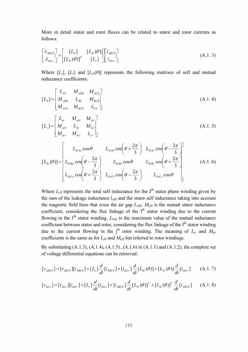
115

More in detail stator and rotor fluxes can be related to stator and rotor currents as

follows:

abcr

ABCS

rT

Sr

SrS

abcr

ABCS

i

i

LL

LL

][)]([

)]([][

(A.1. 3)

Where [Ls], [Lr] and [Lsr(θ)] represents the following matrixes of self and mutual

inductance coefficients:

CSBCSACS

BCSBSABS

ACSABSAS

S

LMM

MLM

MML

L ][ (A.1. 4)

crbcracr

bcrbrabr

bcrabrar

r

LMM

MLM

MML

L ][ (A.1. 5)

cos3

2cos

3

2cos

3

2coscos

3

2cos

3

2cos

3

2coscos

)]([

SrCcSrCbSrCa

SrBcSrBbSrBa

SrAcSrAbSrAa

Sr

LLL

LLL

LLL

L (A.1. 6)

Where LJS represents the total self inductance for the Jth stator phase winding given by

the sum of the leakage inductance lJdS and the stator self inductance taking into account

the magnetic field lines that cross the air gap LJSS. MIJS is the mutual stator inductance

coefficient, considering the flux linkage of the Ith stator winding due to the current

flowing in the Jth stator winding. LSrIj is the maximum value of the mutual inductance

coefficient between stator and rotor, considering the flux linkage of the Ith stator winding

due to the current flowing in the jth rotor winding. The meaning of Ljr and Mijr

coefficients is the same as for LJS and MIJS but referred to rotor windings.

By substituting (A.1.3), (A.1.4), (A.1.5) , (A.1.6) in (A.1.1) and (A.1.2), the complete set

of voltage differential equations can be retrieved:

][)]([)]([][][][]][[][ abcrSrSrabcrABCSsABCSABCSABCS idt

dLL

dt

dii

dt

dLirv (A.1. 7)

][)]([)]([][][][]][[][ ABCST

SrT

SrABCSabcrrabcrabcrabcr idt

dLL

dt

dii

dt

dLirv (A.1. 8)

116

On the hypothesis of null homopolar stator and rotor currents and considering line to

line voltages instead of phase voltages, the six equations (A.1.7) and (A.1.8) can be

reduced to four equations:

br

ar

BS

AS

br

ar

BS

AS

bcr

acr

BCS

ACS

i

i

i

i

dt

dB

i

i

i

i

A

v

v

v

v

)(),( (A.1. 9)

Where matrix [A(θ,ω)] contains all the e.m.f. motional terms, whereas all the

transformer terms are confined in [B(θ)]. For the sake of brevity these two matrixes are

not presented here since they do not add a lot to the discussion, anyway they can be

easily derived from equations (A.1.7) and (A.1.8).

For the simulation of the transient electromechanical state also the two mechanical

equations:

2

em l a

J dT T K

P dt P

(A.1. 10)

d

dt

(A.1. 11)

where J is the moment of inertia Tl is the load torque and the Tem the electromagnetic

torque, has to be added to the system where the Tem can be computed as follows:

][)]([

][ abcrSrT

ABCSem id

LdiT

(A.1. 12)

Once the set of differential equations (A.1.9) has been expressed in the explicit form (i.e.

in the input state output form), and the two mechanical equations (A.1.10) and (A.1.11).

are taken into account, the entire model presents:

• Five inputs, i.e. two stator line to line voltages, two rotor line to line voltages and

the load torque.

• six state variables, i.e. two stator currents, two rotor currents, and two

mechanical variables, the electrical rotor speed and angle.

• six outputs, i.e. the two stator currents in the stator reference frame, two rotor

currents in the rotor reference frame, the electrical rotor speed and the

electromagnetic torque.

It’s worth noting that, since the voltage equations are written in two different reference

frames, the impedance matrixes in (A.1.9) are dependent on the rotor electrical position

angle. Thus to obtain the explicit form of the voltage differential equations set the

matrix [B(θ)] has to be inversed at each simulation step.

117

APPENDIX. 2: MULTIPLE SPACE VECTOR REPRESENTATION

For a given set of 5 real variables 1 5,..., ,...,kx x x a new set of complex variables

0 1 3, ,y y y can be obtained by means of the following symmetrical linear

transformations:

5

01

1

5k

k

y x

(A.2. 1)

5

1

1

2

5

k

kk

y x

, (ρ = 1, 3) (A.2. 2)

where exp 2 / 5j .

Relationships (A.2.1) and (A.2.2) lead to a real variable 0y (zero-sequence

component) and two complex variables 1 3,y y (multiple space vectors).

The inverse transformations are

1

01,3

k

kx y y

, (k = 1, 2, ..., 5) (A.2. 3)

where the symbol “.” represents the scalar product.

According to (A.2.1)-(A.2.3), a general five-phase system can be represented by two

space vectors and the zero-sequence component. The two space vectors are mutually

independent and move arbitrarily in the corresponding α-β planes.

diagnosis and fault detection in electrical machines and

Documents