diapycnal transport and mixing efficiency in stratified ... · diapycnal transport and mixing...
TRANSCRIPT

Diapycnal Transport and Mixing Efficiency in Stratified Boundary Layers nearSloping Topography
LARS UMLAUF AND HANS BURCHARD
Leibniz-Institute for Baltic Sea Research, Warnemunde, Germany
(Manuscript received 28 January 2010, in final form 8 September 2010)
ABSTRACT
The interaction of shear, stratification, and turbulence in boundary layers on sloping topography is in-
vestigated with the help of an idealized theoretical model, assuming uniform bottom slope and homogeneity
in the upslope direction. It is shown theoretically that the irreversible vertical buoyancy flux generated in the
boundary layer is directly proportional to the molecular destruction rate of small-scale buoyancy variance,
which can be inferred, for example, from microstructure observations. Dimensional analysis of the equations
shows that, for harmonic boundary layer forcing and no rotation, the problem is governed by three non-
dimensional parameters (slope angle, roughness number, and ratio of forcing and buoyancy frequencies).
Solution of the equations with a second-moment closure model for the turbulent fluxes reveals the periodic
generation of gravitationally unstable boundary layers during upslope flow, consistent with available obser-
vations. Investigation of the nondimensional parameter space with the help of this model illustrates a sys-
tematic increase of the bulk mixing efficiencies for (i) steep slopes and (ii) low-frequency forcing. Except for
very steep slopes, mixing efficiencies are substantially smaller than the classical value of G 5 0.2.
1. Introduction
Since Munk (1966) suggested that processes near
sloping topography may significantly contribute to basin-
scale mixing, numerous investigations in the ocean, in
lakes, and in the laboratory have provided support for
this idea. Early observations of detached boundary
layers advecting into the ocean’s interior (Armi 1978,
1979a) showed indirect evidence for the effect of bound-
ary mixing that was later supported by turbulence mi-
crostructure measurements, revealing strongly enhanced
dissipation levels in the bottom boundary layer (BBL)
for various sites in the ocean (e.g., Nash et al. 2007;
Rudnick et al. 2003; Lueck and Mudge 1997) and in lakes
(Lemckert et al. 2004; Wuest and Lorke 2003; Gloor et al.
2000). The probably most direct demonstration of the
basin-scale importance of boundary mixing, however,
came from tracer experiments conducted in stratified
basins of different scales, suggesting a dramatic increase
of the vertical spreading rates of the tracer after it had
touched the boundaries (Goudsmit et al. 1997; Ledwell
and Bratkovich 1995; Ledwell and Hickey 1995).
Breaking and shoaling internal waves and bottom
friction caused by near-bottom currents are believed to
be the major energy sources for BBL mixing in strati-
fied basins (Thorpe 2005; Wuest and Lorke 2003). Near
sloping topography, an interesting phenomenon related
to the oscillating shear caused by internal waves or in-
ternal seiching motions has been revealed by a number
of recent measurements in lakes (Lorke et al. 2005,
2008). These data suggest that differential advection due
to the near-bottom vertical shear acting on the upslope
density gradient during upslope flow may create un-
stable stratification, with considerable implications for
turbulence and mixing in the BBL. Similar occurrences
of gravitationally unstable BBLs were found in the
idealized numerical simulations of Slinn and Levine
(1997), who studied mixing caused by cross-slope tidal
currents on sloping topography at low latitudes. Al-
though these studies have clearly shown that convec-
tion provides an important additional energy source for
turbulence with a yet unknown impact on basin-scale
mixing, an investigation of this effect and its implica-
tions for mixing over a broader parameter range is still
lacking.
Corresponding author address: Lars Umlauf, Leibniz-Institute
for Baltic Sea Research, Seestrasse 15, 18119 Warnemunde, Ger-
many.
E-mail: [email protected]
FEBRUARY 2011 U M L A U F A N D B U R C H A R D 329
DOI: 10.1175/2010JPO4438.1
� 2011 American Meteorological Society

Idealized theoretical models of boundary mixing, as-
suming constant diffusivities and homogeneity in the
upslope direction (Phillips 1970; Wunsch 1970; Thorpe
1987), and laboratory experiments (Phillips et al. 1986)
have illustrated that mixing near a sloping boundary
inevitably leads to a tilting of near-bottom isopycnals,
thus setting up an internal pressure gradient that drives
a residual or ‘‘secondary’’ circulation. Garrett (1990, 1991)
recognized that this secondary circulation could have a
crucial feed back on mixing in the BBL in at least two
respects. First, he pointed out that the secondary circu-
lation has a tendency to create stable stratification in the
BBL, thus providing a mechanism for restratification
without requiring an exchange of fluid between the BBL
and the interior. This effect is likely to result in a higher
mixing efficiency and thus in a larger buoyancy flux.
Second, however, as shown by Garrett (1990, 1991), the
vertical advective buoyancy flux associated with the sec-
ondary circulation is expected to be countergradient, thus
reducing the net vertical buoyancy flux. This puzzling
situation is further complicated by the fact that mixing
parameters are tightly coupled to changes in shear and
stratification.
Our aim here is to derive a framework for estimating
the total vertical buoyancy flux in a sloping BBL from
microstructure observations and numerical simulations
that includes the shear-induced generation and destruc-
tion of stratification and its effect on net mixing. Fol-
lowing previous theoretical work (Phillips 1970; Thorpe
1987; Garrett 1990) and idealized modeling studies
(Ramsden 1995a,b), the theory will be based on an ide-
alized geometry with an infinite slope, ignoring flow
variations in the upslope direction. The latter assump-
tion eliminates any ‘‘tertiary’’ flow (e.g., intrusions), re-
sulting from the upslope divergence of the secondary flow,
as one potentially important mechanism for boundary
layer restratification (Garrett et al. 1993; McDougall
1989; Phillips et al. 1986). Nevertheless, the investigations
mentioned above have demonstrated that important in-
sights into the basic mechanisms of boundary mixing can
be gained in particular with such simplified models.
From the equations governing the problem, we will
identify the key nondimensional parameters and explore
the parameter space with the help of a second-moment
turbulence model, similarly to previous boundary mixing
studies by Weatherly and Martin (1978) and Middleton
and Ramsden (1996) that have focused on the effect of
rotation. Because here we focus on the derivation of the
general theoretical framework, the presentation of the
basic mixing mechanisms, and the role of gravitationally
unstable boundary layers for net mixing, we leave the
additional complications due to rotational effects to fu-
ture work.
2. Geometry and governing equations
a. Geometry
We investigate a Boussinesq fluid periodically moving
up and down a uniform slope with slope angle a in an
infinitely deep basin with variable stratification,
N2 5›b
›z, (1)
where z is the vertical coordinate and
b 5�gr � r
0
r0
(2)
is the buoyancy, with r denoting the density, r0 denoting
a constant reference density, and g denoting the accel-
eration of gravity (Fig. 1a). Outside the BBL, we assume
constant vertical stratification (N 5 N‘) and horizontal
isopycnals. Because rotation is ignored, the flow remains
in a plane spanned by the geopotential coordinates x
and z (Fig. 1a).
The geometrical key simplification results from the
assumption that all gradients in the upslope direction are
negligible, except the upslope buoyancy gradient, which
is assumed to be constant (Garrett et al. 1993). Defining
a rotated coordinate system with the x axis pointing up-
slope and the z axis directed normal to the slope (Fig. 1),
we find that the upslope buoyancy gradient is related to
the interior stratification according to
›b
›x5 N2
‘ sina. (3)
The buoyancy gradient normal to the slope,
N2
[›b
›z, (4)
converges to the constant value
N25
›b‘
›z5 N2
‘ cosa for z!‘ (5)
outside the BBL, where b‘ denotes the buoyancy that
would be observed for perfectly horizontal isopycnals
throughout the domain. As indicated in Fig. 1, in general
the isolines of b and b‘ coincide only outside the BBL.
For the given geometry, it is straightforward to derive
a relation between the different forms of the buoyancy
frequency,
N2 5 N2‘ sin2a1 N2 cosa. (6)
330 J O U R N A L O F P H Y S I C A L O C E A N O G R A P H Y VOLUME 41

Because in a perfectly well-mixed BBL the buoyancy
gradient normal to the slope vanishes by definition
(N2[ 0), we conclude from (6) that N2 5 N‘
2 sin2a in the
BBL, illustrating that the terms well mixed and un-
stratified do not coincide (contrary to the situation in
a basin with flat bottom). Outside the BBL, we find
N2
5 N2‘ cosa, which may be inserted into (6) to recover
the trivial case N2 5 N‘2.
b. Governing equations
Under the assumptions mentioned above, the Reynolds-
averaged Boussinesq equations in rotated coordinates
adopt the following simple form:
›u
›t5� 1
r0
›p
›x1 b sina�
›tx
›z,
0 5� 1
r0
›p
›z1 b cosa,
›b
›t1 u
›b
›x5�›G
›z, (7)
where u is the upslope velocity and p is the pressure
minus the pressure in a reference state of rest (Garrett
et al. 1993). The turbulent flux of momentum, tx
5 u9w9
(w is the velocity normal to the slope, the prime denotes
a fluctuating quantity, and the bar denotes the ensemble
average), and the turbulent buoyancy flux, G 5 w9b9,
are computed from a second-moment turbulence model
as described in detail below.
The upslope pressure gradient in (7) can be eliminated
by taking the x derivative of the second relation in (7),
inserting ›b/›x 5 tana ›b‘ /›z obtained from combining
(3) and (5), and integrating with respect to z. This yields
›u
›t5 (b� b
‘)sina 1
›u‘
›t�
›tx
›z,
›b
›t5�uN2
‘ sina� ›G
›z, (8)
where in the buoyancy equation we have used (3) to
express the constant upslope buoyancy gradient (Garrett
et al. 1993), and assume
u 5 0,›b
›z5 0 for z 5 0 (9)
at the lower boundary. The new integration constant
›u‘ /›t appearing in (8) is a function of time, and it plays
the role of a prescribed interior pressure gradient gov-
erning the evolution of the flow outside the BBL. Iden-
tifying this term with a periodic function of time will serve
below as a simple representation of the oscillating pres-
sure gradient due to internal waves. This approach is
completely analogous to that used by Mellor (2002) to
describe BBL turbulence driven by surface waves; to be
valid, waves are required to be long enough to be com-
patible with our assumption of upslope homogeneity.
The first term on the right-hand side of the momentum
budget in (8) represents the internal pressure gradient,
Ip 5 ~b sina, ~b 5 (b� b‘
), (10)
arising from the tendency of tilted isopycnals to relax
back toward their equilibrium positions (indicated by
the gray lines in Fig. 1).
The evolution of the equilibrium buoyancy b‘ appearing
in (8) is computed from the special case of zero mixing,
›b‘
›t1 u
‘N2
‘ sina 5 0, (11)
where the integration starts from a linearly stratified
buoyancy profile corresponding to N 5 N‘ throughout
the domain. The system described by (8), (9), and (11) is
valid for arbitrary slopes in the range 0 # a , p/2 and
provides three equations for the three unknowns u, b,
and b‘.
FIG. 1. Schematic view of a stratified basin with uniform slope.
The thin lines illustrate isopycnals for the case of mixing (black)
and no mixing (gray) in the BBL. The double arrow indicates the
direction of the bottom-parallel oscillating flow. Shown is the sys-
tem (a) in geopotential coordinates and (b) in rotated, bottom-
parallel coordinates.
FEBRUARY 2011 U M L A U F A N D B U R C H A R D 331
3. Description of turbulence and mixing
a. Turbulent fluxes
The turbulent fluxes of momentum and buoyancy
appearing in (8) are computed from the second-moment
turbulence closure model by Canuto et al. (2001), ex-
tended here by two prognostic equations for the turbu-
lent kinetic energy (TKE) k and the dissipation rate «,
as described in Umlauf and Burchard (2005). This model
is particularly suited for our study because (i) it does not
contain dimensional parameters, which is a crucial re-
quirement for the derivation of the nondimensional
expressions discussed in section 4, and (ii) it does not
contain any assumptions about the vertical structure of
the bottom boundary layer. For these reasons, a number
of frequently used parameterizations for ocean mixing
are not applicable here (e.g., Durski et al. 2004; Large
et al. 1994; Pacanowsci and Philander 1981).
From previous comparison with LES and laboratory
data (Umlauf and Burchard 2005; Umlauf 2009) and
turbulence measurements in entraining boundary layer
flows (e.g., Arneborg et al. 2007; Umlauf et al. 2010), we
expect that the model used here reproduces the basic
interaction mechanisms between shear, stratification, and
turbulence and thus yields credible estimates and correct
trends for the mixing parameters.
It should be emphasized that the derivation of the
second-moment equations for geophysical boundary layers
typically involves two assumptions that conflict with the
applicability of the resulting models for arbitrary slopes:
(i) horizontal gradients of mean quantities in the second-
moment equations are ignored, and (ii) the mean shear
and gravity vectors are assumed to be aligned and vertical
(Mellor and Yamada 1982; Canuto et al. 2001; Umlauf
et al. 2005). Clearly, for the given geometry, these ap-
proximations are justified only for a� 1. Therefore, we
restrict our following investigations to a # 0.1, which
does, however, not impose a serious constraint for the
typical slopes observed in the ocean and in lakes.
Under these conditions, the turbulent fluxes are com-
puted from
tx
5 u9w9 5�ntS, G 5 w9b9 5�nb
t N2,
B 5 w9b9 5�nbt N2, (12)
where S 5 ›u/›z is the shear and nt and vtb are the tur-
bulent diffusivities computed from the second-moment
turbulence model. We distinguish between vertical (B)
and slope-normal (G) buoyancy fluxes, which is essential
for the correct timing of the transition from weakly stable
stratification to convection. Note that, by construction,
the boundary layer turbulence model used here does not
provide an expression for the upslope diffusivity, which
we therefore ignore in the following. This is justified
because (i) shear dispersion as an important upslope
transport mechanism is taken into account and (ii) the
vertical component of the upslope turbulent flux is
likely to be negligible for the small slopes considered
here (a� 1) unless stratification is extremely weak or
the upslope diffusivity is extremely large (Garrett et al.
1993).
The second-moment equations lead to the following
expressions for the turbulent diffusivities (Canuto et al.
2001; Umlauf and Burchard 2005):
nt5 c
m
k2
«, nb
t 5 cbm
k2
«, (13)
where, using the ‘‘quasi equilibrium’’ assumption of
Galperin et al. (1988), the stability functions, cm and cmb
can be shown to depend only on the dimensionless
buoyancy number Nk/«.
Different from Canuto et al. (2001), we do not as-
sume that the TKE equation is in equilibrium, and we
solve the full transport equation,
›k
›t� ›
›z
nt
sk
›k
›z
� �5 P 1 B� «, (14)
where P 5 ntS2 denotes the shear production. The dis-
sipation rate is computed from a transport equation of
the form
›«
›t� ›
›z
nt
s«
›«
›z
� �5
«
k(c
1P 1 c
3B� c
2«), (15)
with all model parameters summarized in Table 1.
Using the boundary conditions ›k/›z 5 0 and « 5 uf3/
(kz0) at z 5 0, where uf2 5 jtxjz50 denotes the square of
the friction velocity, z0 denotes the bottom roughness
length, and k denotes the von Karman constant (see
Table 1), it can be shown that the velocity follows the
expected logarithmic wall profile,
juj5u
f
kln
z 1 z0
z0
� �, z! 0. (16)
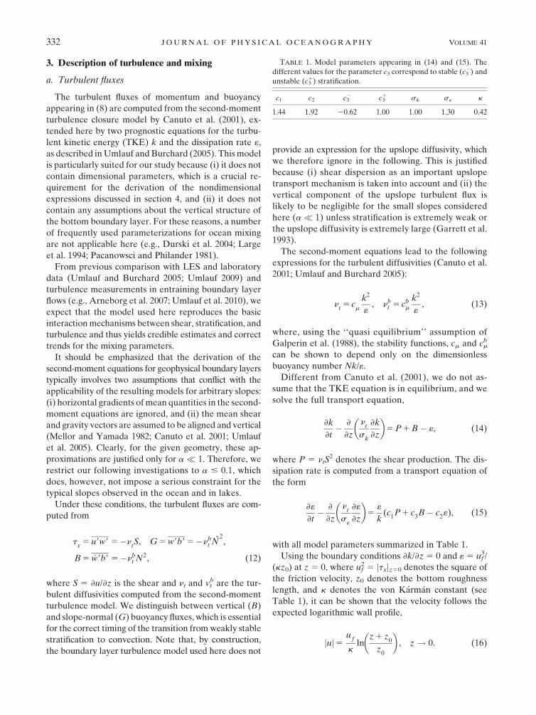
TABLE 1. Model parameters appearing in (14) and (15). The
different values for the parameter c3 correspond to stable (c32) and
unstable (c31) stratification.
c1 c2 c32 c3
1 sk s« k
1.44 1.92 20.62 1.00 1.00 1.30 0.42
332 J O U R N A L O F P H Y S I C A L O C E A N O G R A P H Y VOLUME 41

Note that all boundary conditions are imposed at the
‘‘virtual origin’’ (z 5 0) of the logarithmic profile in (16),
where u 5 0 consistent with (9). Details and numerical
implementation are described, for example, in Burchard
et al. (2005).
b. Quantification of mixing
To derive the framework for a precise definition of mix-
ing, we start from the equation for the variance of turbulent
buoyancy fluctuations b92 (Tennekes and Lumley 1972;
Umlauf and Burchard 2005). With the geometrical con-
straints described in section 2 (but without any turbulence
modeling assumptions), this equation can be written as
›b92
›t5�
›Fb
›z1 P
b� x
b, (17)
where Fb denotes the sum of the turbulent and viscous
transport terms [the exact form of Fb is given, e.g., in Eq.
(A.3) of Umlauf and Burchard 2005]. For our idealized
geometry, the production term is of the form
Pb
5�2u9b9›b
›x� 2w9b9
›b
›z
5 2u9b9N2‘ sin a� 2GN
2(18)
and the destruction of small-scale buoyancy variance by
molecular mixing is given by
xb
5 2nb›b9
›xi
›b9
›xi
, (19)
where nb is the molecular diffusivity of buoyancy (cor-
responding to that of either heat or salt), and we sum
over i 5 1, 2, 3 with the xi corresponding to some arbi-
trary orthogonal coordinate system. The destruction
rate xb in (19) is positive by definition and describes the
molecular, irreversible mixing of fluid with different
densities. This quantity is of central importance for the
following analysis because, as discussed in detail below,
it is closely related to the irreversible vertical buoyancy
flux in the BBL.
Finally, it is important to note that the turbulence
model by Canuto et al. (2001) used for our numerical
simulations employs the equilibrium version of (17):
Pb 5 xb. Consistent with the boundary layer approxi-
mation discussed in the previous section, the production
of buoyancy variance in (18) is dominated by vertical
stratification: that is, Pb 5 22BN2 (see Canuto et al.
2001), which is a good approximation for both the total
and slope-normal production as long as a � 1. With
these assumptions, the equilibrium form of (17) reduces
to the familiar Osborn–Cox model that is frequently
used for the interpretation of oceanic microstructure
data (Osborn and Cox 1972; Gregg 1987). It is worth
pointing out that the integral of the flux term Fb in (17)
vanishes because (i) there is no mixing outside the BBL
and (ii) it can be shown that Fb 5 0 at z 5 0 because
there is no buoyancy flux through the lower boundary
(Umlauf and Burchard 2005). Much of the following
analysis is based on time-averaged, vertically integrated
equations for periodic flows (for which the rate terms
vanish as well), such that the equilibrium assumption
does not imply any restrictions.
4. Nondimensional description
We start our nondimensional analysis from (8), re-
written in the form
›u
›t5 eb sina 1
›u‘
›t�
›tx
›z,
›eb›t
5�(u� u‘
)N2‘ sina� ›G
›z, (20)
where we used (11) to derive an equation for eb defined
in (10).
As a simple representation of internal-wave forcing,
we assume that the outer flow is purely harmonic,
u‘
5U sinvt, (21)
where U denotes a constant velocity scale and v denotes
the forcing frequency. This relationship introduces the
characteristic time scale v21 to the problem, which we
use to nondimensionalize the time according to
t* 5 tv, (22)
where here and in the following the asterisk denotes a
nondimensional variable. From (20), we identify the
slope angle a and the background stratification N‘ as
independent parameters. The parameters U and v are
introduced by the forcing term in (21), and the bottom
roughness z0 enters the problem via the boundary con-
dition for the dissipation rate discussed in the context
of (15).
With these parameters, we nondimensionalize the
vertical coordinate as
z* 5zN
‘
U(23)
and introduce the nondimensional variables
FEBRUARY 2011 U M L A U F A N D B U R C H A R D 333
u* 5u
U, eb* 5
ebUN
‘
, tx* 5
tx
U2, «* 5
«
U2N‘
,
G* 5G
U2N‘
. (24)
The nondimensional form of (20) is thus
V›u*
›t*5 eb* sina 1 V cos t*�
›tx*
›z*,
V›eb*
›t*5�(u*� sin t*)sina� ›G*
›z*, (25)
where we have defined the nondimensional frequency,
V 5v
N‘
. (26)
Using the nondimensional friction velocity uf* 5 uf /U,
the boundary condition for « becomes
«* 5(u
f*)3
kRfor z* 5 0, (27)
which introduces the last nondimensional key quantity:
the roughness parameter,
R 5z
0N
‘
U. (28)
For harmonic forcing, the parameter space is thus
spanned be three independent quantities, a, R, and V.
It is straightforward to show that the equations for the
turbulent quantities in (13), (14), and (15) can be made
dimensionless in a similar way without introducing any
new nondimensional parameters. Note that the exis-
tence of three independent nondimensional parameters
also follows directly from combining the five dimen-
sional parameters governing the problem (a, U, v, N‘,
and z0) into nondimensional products.
5. Properties
a. Shear-induced stratification
The effect of the shear, S 5 ›u/›z, on vertical strati-
fication inside the BBL is easiest understood from the
transport equation of the buoyancy frequency,
›N2
›t5 �SN2
‘ sina� ›2G
›z2
� �cosa, (29)
which is derived from the time derivative of (6), insert-
ing the z derivative of the buoyancy equation in (8).
From (29), negative near-bottom shear (downslope
flow) is seen to have a tendency to enhance stratification.
The impact of this effect on mixing is, however, not ob-
vious because there are two competing feedback mech-
anisms: (i) the suppression of turbulence due to the
generation of stable stratification and (ii) the enhance-
ment of mixing due to an increase of the mixing effi-
ciency (e.g., Shih et al. 2005). Conversely, for positive
near-bottom shear (upslope flow), stratification is de-
stroyed, which may ultimately lead to unstable stratifi-
cation, thus providing an additional energy source in
the TKE budget (14). The relative importance of these
effects will be studied in detail below.
b. Boundary layer resonance
An equation for the boundary layer velocity relative
to the interior flow, ~u 5 u� u‘
, can be obtained from
the time derivative of the momentum equation in (20),
inserting the buoyancy equation in (20) on the right-
hand side. After some rearrangement, this yields
›2 ~u
›t21 ~uN2
‘ sin2a 5�›G
›zsina�
›2tx
›z›t, (30)
where the left-hand side is recognized as that of a har-
monic oscillator with resonance at the critical frequency
vc 5 N‘sina. This generalizes a similar result derived
by Thorpe (1987) for piecewise constant diffusivities,
leading to the interesting conclusion that boundary layer
resonance is reached for the frequency at which internal
waves are critically reflected from the slope (e.g., Thorpe
and Umlauf 2002).
c. Residual transport
In the following, expressions for the residual volume
and buoyancy fluxes are obtained, either from periodic
averages for harmonic forcing or by integrating over an
arbitrary ‘‘mixing event’’ of finite duration, assuming that,
before the event (t , t1) and after (t . t2), the boundary
layer has fully restratified and returned to a state of rest
with u 5 0 and horizontal isopycnals (b 5 b‘).
Assuming negligible mixing outside the BBL, in-
tegration of the buoyancy equation in (8) from the
bottom to an arbitrary reference level, z 5 zr, outside
the BBL yields
d
dt
ðzr
0
b dz 5�QN2‘ sina, Q [
ðzr
0
u dz, (31)
where we have used the facts that G 5 0 at the bottom
and no mixing occurs outside the BBL. Integrating (31)
from t1 to t2 over a mixing event, the left-hand side
vanishes, and thus there is no net transport, irrespective
334 J O U R N A L O F P H Y S I C A L O C E A N O G R A P H Y VOLUME 41
of the nature of the event and the value of zr. Similarly,
for monochromatic forcing, (21), and fully periodic flow
we find
hQi5 1
T
ðt1T
t
Q(t) dt 5 0 (periodic flow), (32)
where we have introduced the symbol h� � �i to denote the
average over one period, T 5 2p/v. This generalizes the
result derived by Phillips (1970) for stationary flows with
zero mixing outside the BBL. Note that in (32) and all
following results, the averaging procedure removes any
dependency on the reference level zr.
For periodic flow, the vertical structure of the residual
currents follows from averaging the buoyancy equation
in (8),
hui5 h~ui5� 1
N2‘ sina
›hGi›z
(for periodic flow). (33)
Because hGi5 0 at the bottom, it is clear from (33) that,
for hGi , 0 near the bottom, the residual near-bottom
circulation will be upslope, consistent with the available
analytical solutions for constant or piecewise constant
diffusivities summarized by Garrett (1990, 1991) and
Garrett et al. (1993). Conversely, for hGi . 0 (i.e., con-
vection dominates), we expect a reversal of the near-
bottom circulation.
To obtain an expression for the residual upslope buoy-
ancy flux, we start from the evolution equation for the
square of the buoyancy b2, which is easily derived by
multiplying the buoyancy equation in (8) with b. The
result is integrated across the BBL and added to the
integral of the equation for the buoyancy variance, (17).
Using (18) for the production term and the fact that Fb
vanishes at the integration limits (see above), this finally
yields
d
dt
ðzr
0
(b2 1 b92) dz 5�2QbN2
‘ sina�H, (34)
where we have introduced
Qb
[
ðzr
0
(ub 1 u9b9) dz and H[
ðzr
0
xb
dz (35)
for the total (i.e., advective plus turbulent) upslope
buoyancy flux and the integrated mixing rate, respectively.
It is evident from (34) that the instantaneous upslope
buoyancy flux Qb results from mixing (last term on the
right-hand side), as well as from temporal variations
of the variance terms on the left-hand side. The latter
terms, however, vanish if integrated over an arbitrary
mixing event as described above, and (34) thus yields
ðt2
t1
Qb
dt 5
ðt2
t1
Qirrb dt, Qirr
b 5� H2N2
‘ sina# 0, (36)
relating the irreversible buoyancy flux to the mixing
rate. Similarly, for periodic forcing and fully periodic
flow, averaging (34) over one period yields
hQbi5 hQirr
b i,
hQirrb i5�
hHi2N2
‘ sina# 0, (for periodic flow). (37)
Note that the local buoyancy b is only known up to an
arbitrary constant b0, which implies that the averaged
advective buoyancy flux,
hu(b 1 b0)i5 hubi1 huib
0, (38)
contains an arbitrary component that is proportional
to the averaged speed hui. For fully periodic conditions,
however, hQbi becomes independent of the reference
buoyancy because the vertical integral of hui vanishes
according to (32).
It should be noted that both relations, (36) and (37),
imply that the irreversible buoyancy flux is strictly down-
slope and thus associated with an irreversible increase of
potential energy due to mixing. To quantify this important
conclusion, we exploit the fact that hQbi, the total upslope
buoyancy flux integrated over a line normal to the slope
coincides with the total vertical buoyancy flux integrated
over a horizontal line. To see this, we note that, analo-
gous to the derivation for stationary flows (Garrett 1991;
Garrett et al. 1993), for periodic flows it can be shown that
hQbi5ð0
�‘
hubisina dx 1
ð0
�‘
hGicosa dx
1
ð0
�‘
hu9b9isina dx, (39)
where we have arbitrarily chosen a position on the slope
that coincides with the origin of the coordinate systems
shown in Fig. 1. The terms on the right-hand side of (39)
are recognized as (i) the vertical advective flux, (ii) the
vertical component of the slope-normal turbulent flux,
and (iii) the vertical component of the upslope turbulent
flux. The sum of the latter two terms thus corresponds to
the total vertical turbulent flux, referred to as hQGi in
the following.
With the interpretation of hQbi as the total vertical
buoyancy flux, (36) and (37) form one of the key results
FEBRUARY 2011 U M L A U F A N D B U R C H A R D 335
of this paper, linking the molecular fluxes at the smallest
(Batchelor) scales of the flow to the large-scale net buoy-
ancy flux and thus to the change of background potential
energy (Winters et al. 1995). In this context, it is worth
pointing out that, based on an analysis of a similar prob-
lem in isopycnal coordinates, Garrett (2001) arrived at the
related conclusion that only the turbulent buoyancy flux
across mean isopycnals (i.e., the mean diapycnal flux) has
an effect on the net vertical buoyancy flux.
Note that no turbulence modeling assumptions are
involved in the derivation of these results. Also note that
(36) and (37) are valid also for rotating flows because the
momentum equation is not used in their derivation.
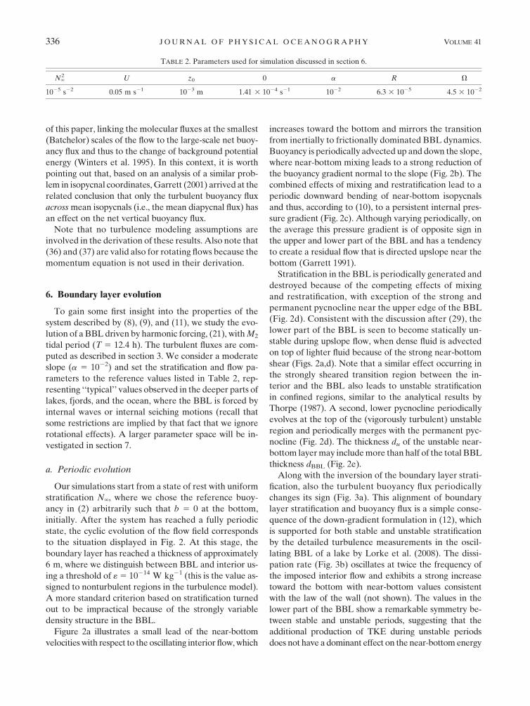
6. Boundary layer evolution
To gain some first insight into the properties of the
system described by (8), (9), and (11), we study the evo-
lution of a BBL driven by harmonic forcing, (21), with M2
tidal period (T 5 12.4 h). The turbulent fluxes are com-
puted as described in section 3. We consider a moderate
slope (a 5 1022) and set the stratification and flow pa-
rameters to the reference values listed in Table 2, rep-
resenting ‘‘typical’’ values observed in the deeper parts of
lakes, fjords, and the ocean, where the BBL is forced by
internal waves or internal seiching motions (recall that
some restrictions are implied by that fact that we ignore
rotational effects). A larger parameter space will be in-
vestigated in section 7.
a. Periodic evolution
Our simulations start from a state of rest with uniform
stratification N‘, where we chose the reference buoy-
ancy in (2) arbitrarily such that b 5 0 at the bottom,
initially. After the system has reached a fully periodic
state, the cyclic evolution of the flow field corresponds
to the situation displayed in Fig. 2. At this stage, the
boundary layer has reached a thickness of approximately
6 m, where we distinguish between BBL and interior us-
ing a threshold of « 5 10214 W kg21 (this is the value as-
signed to nonturbulent regions in the turbulence model).
A more standard criterion based on stratification turned
out to be impractical because of the strongly variable
density structure in the BBL.
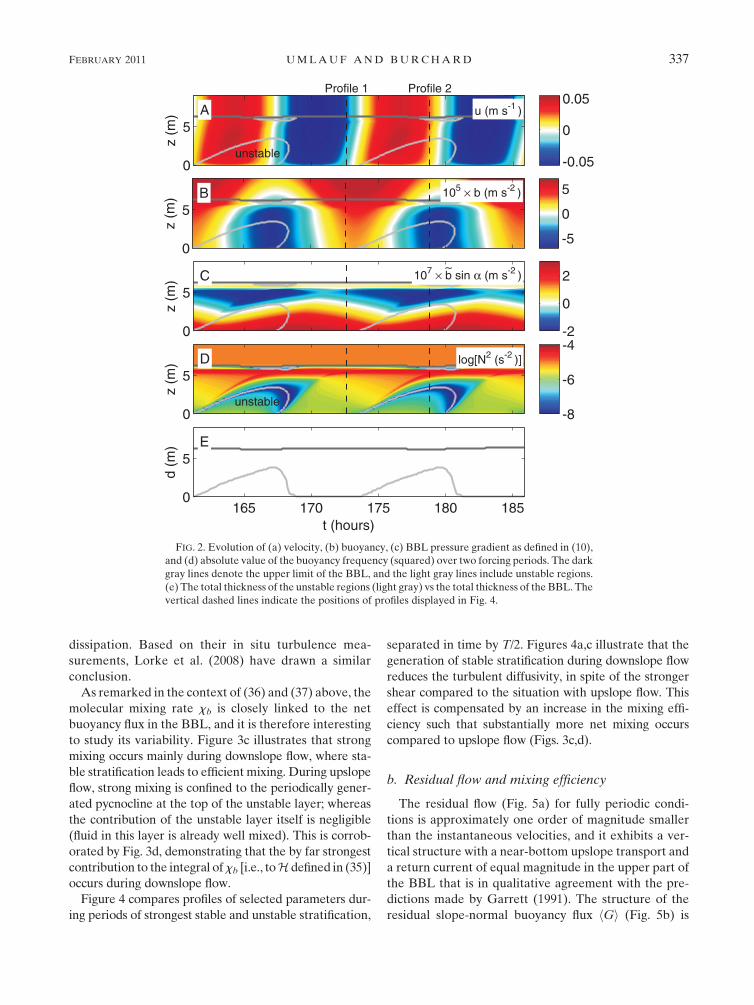
Figure 2a illustrates a small lead of the near-bottom
velocities with respect to the oscillating interior flow, which
increases toward the bottom and mirrors the transition
from inertially to frictionally dominated BBL dynamics.
Buoyancy is periodically advected up and down the slope,
where near-bottom mixing leads to a strong reduction of
the buoyancy gradient normal to the slope (Fig. 2b). The
combined effects of mixing and restratification lead to a
periodic downward bending of near-bottom isopycnals
and thus, according to (10), to a persistent internal pres-
sure gradient (Fig. 2c). Although varying periodically, on
the average this pressure gradient is of opposite sign in
the upper and lower part of the BBL and has a tendency
to create a residual flow that is directed upslope near the
bottom (Garrett 1991).
Stratification in the BBL is periodically generated and
destroyed because of the competing effects of mixing
and restratification, with exception of the strong and
permanent pycnocline near the upper edge of the BBL
(Fig. 2d). Consistent with the discussion after (29), the
lower part of the BBL is seen to become statically un-
stable during upslope flow, when dense fluid is advected
on top of lighter fluid because of the strong near-bottom
shear (Figs. 2a,d). Note that a similar effect occurring in
the strongly sheared transition region between the in-
terior and the BBL also leads to unstable stratification
in confined regions, similar to the analytical results by
Thorpe (1987). A second, lower pycnocline periodically
evolves at the top of the (vigorously turbulent) unstable
region and periodically merges with the permanent pyc-
nocline (Fig. 2d). The thickness du of the unstable near-
bottom layer may include more than half of the total BBL
thickness dBBL (Fig. 2e).
Along with the inversion of the boundary layer strati-
fication, also the turbulent buoyancy flux periodically
changes its sign (Fig. 3a). This alignment of boundary
layer stratification and buoyancy flux is a simple conse-
quence of the down-gradient formulation in (12), which
is supported for both stable and unstable stratification
by the detailed turbulence measurements in the oscil-
lating BBL of a lake by Lorke et al. (2008). The dissi-
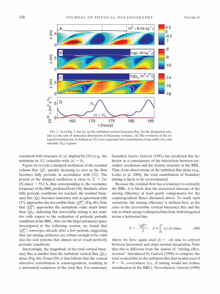
pation rate (Fig. 3b) oscillates at twice the frequency of
the imposed interior flow and exhibits a strong increase
toward the bottom with near-bottom values consistent
with the law of the wall (not shown). The values in the
lower part of the BBL show a remarkable symmetry be-
tween stable and unstable periods, suggesting that the
additional production of TKE during unstable periods
does not have a dominant effect on the near-bottom energy
TABLE 2. Parameters used for simulation discussed in section 6.
N‘2 U z0 0 a R V
1025 s22 0.05 m s21 1023 m 1.41 3 1024 s21 1022 6.3 3 1025 4.5 3 1022
336 J O U R N A L O F P H Y S I C A L O C E A N O G R A P H Y VOLUME 41
dissipation. Based on their in situ turbulence mea-
surements, Lorke et al. (2008) have drawn a similar
conclusion.
As remarked in the context of (36) and (37) above, the
molecular mixing rate xb is closely linked to the net
buoyancy flux in the BBL, and it is therefore interesting
to study its variability. Figure 3c illustrates that strong
mixing occurs mainly during downslope flow, where sta-
ble stratification leads to efficient mixing. During upslope
flow, strong mixing is confined to the periodically gener-
ated pycnocline at the top of the unstable layer; whereas
the contribution of the unstable layer itself is negligible
(fluid in this layer is already well mixed). This is corrob-
orated by Fig. 3d, demonstrating that the by far strongest
contribution to the integral of xb [i.e., toH defined in (35)]
occurs during downslope flow.
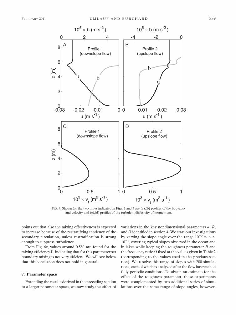
Figure 4 compares profiles of selected parameters dur-
ing periods of strongest stable and unstable stratification,
separated in time by T/2. Figures 4a,c illustrate that the
generation of stable stratification during downslope flow
reduces the turbulent diffusivity, in spite of the stronger
shear compared to the situation with upslope flow. This
effect is compensated by an increase in the mixing effi-
ciency such that substantially more net mixing occurs
compared to upslope flow (Figs. 3c,d).
b. Residual flow and mixing efficiency
The residual flow (Fig. 5a) for fully periodic condi-
tions is approximately one order of magnitude smaller
than the instantaneous velocities, and it exhibits a ver-
tical structure with a near-bottom upslope transport and
a return current of equal magnitude in the upper part of
the BBL that is in qualitative agreement with the pre-
dictions made by Garrett (1991). The structure of the
residual slope-normal buoyancy flux hGi (Fig. 5b) is
FIG. 2. Evolution of (a) velocity, (b) buoyancy, (c) BBL pressure gradient as defined in (10),
and (d) absolute value of the buoyancy frequency (squared) over two forcing periods. The dark
gray lines denote the upper limit of the BBL, and the light gray lines include unstable regions.
(e) The total thickness of the unstable regions (light gray) vs the total thickness of the BBL. The
vertical dashed lines indicate the positions of profiles displayed in Fig. 4.
FEBRUARY 2011 U M L A U F A N D B U R C H A R D 337
consistent with structure of hui implied by (33) (e.g., the
minimum in hGi coincides with hui 5 0).
Figure 6a reveals a damped oscillation of the residual
volume flux hQi, quickly decaying to zero as the flow
becomes fully periodic in accordance with (32). The
period of the damped oscillation is close to Tc 5 2p/
(N‘sina) 5 55.2 h, thus corresponding to the resonance
frequency of the BBL predicted from (30). Similarly, when
fully periodic conditions are reached, the residual buoy-
ancy flux hQbi becomes stationary and, in agreement with
(37), approaches the irreversible limit, hQirrb i (Fig. 6b). Note
that hQirrb i approaches the asymptotic value much faster
than hQbi, indicating that irreversible mixing is not sensi-
tive with respect to the realization of perfectly periodic
conditions in the BBL. Also, for the larger parameter space
investigated in the following section, we found that
hQirrb i converges already after a few periods, suggesting
that our mixing estimates are robust enough to be valid
also for real systems that almost never reach perfectly
periodic conditions.
Interestingly, the magnitude of the total vertical buoy-
ancy flux is smaller than the turbulent vertical flux hQGialone (Fig. 6b). From (39), it thus follows that the vertical
advective contribution is countergradient, resulting in
a substantial reduction of the total flux. For stationary
boundary layers, Garrett (1991) has predicted this be-
havior as a consequence of the interaction between sec-
ondary circulation and the density structure in the BBL.
Thus, from observations of the turbulent flux alone (e.g.,
Lorke et al. 2008), the total contribution of boundary
mixing is likely to be overestimated.
Because the residual flow has a tendency to restratify
the BBL, it is likely that the associated increase of the
mixing efficiency at least partly compensates for the
countergradient fluxes discussed above. To study such
variations, the mixing efficiency is defined here as the
ratio of the irreversible vertical buoyancy flux and the
rate at which energy is dissipated into heat, both integrated
across a horizontal line:
G 5�hQirrb iE , E[
ð‘
0
h«i dz/sina, (40)
where we have again used dz 5 �dx sina to convert
between horizontal and slope-normal integration. Note
that this is different from the notion of ‘‘mixing effec-
tiveness’’ introduced by Garrett (1990) to compare the
total vertical flux to the turbulent flux that would occur if
N 5 N‘ everywhere (i.e., if mixing would not reduce
stratification in the BBL). Nevertheless, Garrett (1990)
FIG. 3. As in Fig. 2, but for (a) the turbulent vertical buoyancy flux, (b) the dissipation rate,
and (c) the rate of molecular destruction of buoyancy variance. (d) The evolution of the in-
tegrated mixing rateH defined in (35), here separated into contributions from stable (Hs) and
unstable (Hu) regions.
338 J O U R N A L O F P H Y S I C A L O C E A N O G R A P H Y VOLUME 41
points out that also the mixing effectiveness is expected
to increase because of the restratifying tendency of the
secondary circulation, unless restratification is strong
enough to suppress turbulence.
From Fig. 6c, values around 0.5% are found for the
mixing efficiency G, indicating that for this parameter set
boundary mixing is not very efficient. We will see below
that this conclusion does not hold in general.
7. Parameter space
Extending the results derived in the preceding section
to a larger parameter space, we now study the effect of
variations in the key nondimensional parameters a, R,
and V identified in section 4. We start our investigations
by varying the slope angle over the range 1023 # a #
1021, covering typical slopes observed in the ocean and
in lakes while keeping the roughness parameter R and
the frequency ratio V fixed at the values given in Table 2
(corresponding to the values used in the previous sec-
tion). We resolve this range of slopes with 200 simula-
tions, each of which is analyzed after the flow has reached
fully periodic conditions. To obtain an estimate for the
effect of the roughness parameter, these experiments
were complemented by two additional series of simu-
lations over the same range of slope angles, however,
FIG. 4. Shown for the two times indicated in Figs. 2 and 3 are (a),(b) profiles of the buoyancy
and velocity and (c),(d) profiles of the turbulent diffusivity of momentum.
FEBRUARY 2011 U M L A U F A N D B U R C H A R D 339

with R one order of magnitude larger and smaller than
the value mentioned in Table 2. For each simulation, we
computed the irreversible buoyancy flux Qirrb
� �from
(37). As theoretically shown in (37) and numerically
verified in Fig. 6b, for periodic conditions Qirrb
� �con-
verges to the total vertical buoyancy flux hQbi. The
contribution of the upslope turbulent flux in (39) turned
out to be negligible in all our simulations. Note that we
do not discuss model predictions in the immediate vi-
cinity of the critical value for BBL resonance (gray-
shaded areas in Figs. 7, 8) because there (i) fully periodic
conditions are reached only after an unrealistically large
number of periods and (ii) near-critical reflection of
internal waves occurring for a ’ ac is hardly compatible
with the geometric assumptions outlined in section 2.
As illustrated in Figs. 7a,b, the nondimensional total
and turbulent buoyancy fluxes, hQb*i 5 hQbi/U3 and
hQG*i 5 hQGi/U3, show a systematic increase for in-
creasing roughness numbers R over the whole spectrum
of slopes. However, given that both R and a vary by two
orders of magnitude, the overall variability of the non-
dimensional buoyancy fluxes is surprisingly small with
typical values on the order of hQb*i ’ 1023, except near
the critical slope, where both fluxes collapse.
For a , ac, we find that the magnitude of the total flux
hQb*i is generally smaller than the magnitude of the
turbulent flux hQG*i. Similar to the observations made
in the context of Fig. 6b, this implies that the vertical
advective flux is countergradient and may lead to a sub-
stantial reduction of the total flux. Because the two-layer
structure of the secondary circulation remains qualita-
tively similar to that shown in Fig. 5a for subcritical slopes,
FIG. 5. Residual profiles of (a) the upslope velocity and (b) the slope-normal turbulent buoy-
ancy flux, with both shown for fully periodic conditions.
FIG. 6. Time series of (a) the volume flux, (b) different contribu-
tions to the vertical buoyancy flux, and (c) bulk mixing efficiency. All
quantities are averaged over one period. The gray-shaded areas
correspond to the period shown in Figs. 2 and 3.
340 J O U R N A L O F P H Y S I C A L O C E A N O G R A P H Y VOLUME 41

these results support the suggestion of Garrett (1990,
1991) that the advective contribution of the secondary
circulation results in a reduction of the total vertical
buoyancy flux. For supercritical slopes, a , ac, however,
we observe a reversal of the secondary circulation (not
shown), with the consequence that both the turbulent
and the advective vertical fluxes change their signs (Figs.
7a,b).
As shown in Figs. 7c,d, the nondimensional dissipa-
tion rate hE*i 5 hEi/U3 and the bulk mixing efficiency G
defined in (40) are weak functions of the roughness pa-
rameter R but exhibit strong, opposing trends for in-
creasing slope angle a. The strong decrease of the
dissipation rate over the range of slopes investigated
here can be understood from the following argument:
The dissipation rate integrated in the slope-normal di-
rection across the BBL can be expressed as CDU3, where
CD is a (not necessarily constant) dimensionless drag
coefficient. Thus, using (40), we find a simple non-
dimensional relationship of the form hE*i sina 5 CD,
where the appearance of the trigonometric factor mir-
rors the conversion from horizontal to slope-normal in-
tegration. The drag coefficient exhibits little variability
in our simulations, which can be explained from the
fact that most of the dissipation rate occurs very close to
the bottom in a region that is not strongly affected by
stratification (see Fig. 3b). Hence, for constant CD, an
inverse relationship between hE*i and the slope angle is
expected.
This is largely consistent with the behavior of hE*idisplayed in Fig. 7c, from which we also infer CD 5
O(1023), slightly variable for different roughness num-
bers but well inside the range of accepted values. The
mixing efficiency increases from values less than G 5
1023 for mild slopes up to efficiencies larger than 1% for
slope angles exceeding a 5 (1–2) 3 1022. This trend is
consistent with the observations of Gloor et al. (2000),
who carefully analyzed the energy budget of a small lake
and reported increasing mixing efficiencies for steeper
slopes.
The role played by the secondary circulation in this
process can be understood from averaging the evolution
FIG. 7. Nondimensional, periodically averaged parameters as
functions of the slope angle a for V 5 4.5 3 1022 and roughness
numbers R 5 6.3 3 1026 (dotted lines), R 5 6.3 3 1025 (dashed
lines), and R 5 6.3 3 1024 (solid lines). Increasing values of R are
indicated by the arrow. Shown are (a) total vertical buoyancy flux,
(b) turbulent vertical buoyancy flux, (c) integrated dissipation rate,
(d) bulk mixing efficiency, and (e) standard deviation of secondary
circulation. Vertical dashed lines mark the critical slope with gray
area indicating the near-critical region 0.9ac # a # 1.1ac.
FIG. 8. Nondimensional, periodically averaged parameters as
functions of the nondimensional frequency V for a 5 1022 and R 5
6.3 3 1025. Shown are (a) total (solid line) and turbulent (dashed
line) vertical buoyancy flux, (b) bulk mixing efficiency, (c) total
BBL and unstable layer thicknesses, and (d) standard deviation of
secondary circulation. The vertical dashed lines mark the critical
frequency with gray area indicating the near-critical region 0.9Vc #
V # 1.1Vc.
FEBRUARY 2011 U M L A U F A N D B U R C H A R D 341

equation for N2 in (29) over one period. Assuming pe-
riodic conditions, the rate term vanishes, and the shear
and mixing terms on the right-hand side must balance.
Because negative residual shear, hSi, 0, is seen to have
a tendency to generate stable stratification (here in the
core of the BBL; see Fig. 5a), a compensation by the
second term on the right-hand side of (29) (i.e., by mix-
ing) is required to insure that hN2i remains constant.
However, because the shear term in (29) is proportional
to the upslope buoyancy gradient, N‘2 sin a, we expect
that the generation of stable stratification occurs at a
higher rate for steeper slopes. The magnitude of the sec-
ondary circulation, defined here as the (nondimensional)
standard deviation of the residual flow su* 5 su/U, is on
the order of a few percent of the interior flow and shows
relatively little variability for varying slope angles (Fig.
7e). The rate at which stable stratification inside the
BBL is generated thus depends to a large extent on the
upslope density gradient, which increases for steeper
slopes.
The net stabilizing effect of the secondary circulation
is mirrored in an increased mixing efficiency (Fig. 7d) but,
as shown by our results, also in a suppression of turbu-
lence (Fig. 7c) for steeper slopes. Both effects nearly can-
cel, and the net impact on the total buoyancy flux (Fig. 7a)
is comparatively small. This is one of the key results of
this section.
Similarly to the above analysis, we isolate the effects
of variable forcing frequency V for fixed R and a (see
Table 2) with 200 simulations spanning a range of two
orders of magnitude around the reference value for V
given in Table 2. Values outside this range are either too
close to the upper limit for internal waves (v 5 N) to be
compatible with the geometrical assumptions made in
section 2 or describe wave frequencies that are too small
to reach fully periodic conditions on realistic time scales.
The key information obtained from these simulations
is that both the buoyancy flux (Fig. 8a) and the mixing
efficiency (Fig. 8b) become vanishingly small in the high-
frequency limit. This behavior can be understood by re-
calling from the discussion of Figs. 3c,d that mixing is
mainly associated with phases of downslope flow, where
shear-induced stable stratification leads to more efficient
mixing. For high-frequency forcing, however, increasingly
shorter periods of downslope flow inhibit the full devel-
opment of this process.
The nondimensional thickness, hdu*i 5 hduiN‘/U, of
the unstable layer is only a small fraction of the total
layer thickness, hd*BBLi 5 hd
BBLiN
‘/U, but convection
is seen to occur for all frequencies (Fig. 8c). In fact, in all
our simulations we observed periods with unstable
boundary layers, suggesting that this phenomenon is an
intrinsic component of the BBL dynamics, at least in the
nonrotating case. The secondary circulation (Fig. 8e)
remains in the range of 1%–3% of the interior flow U
over the whole frequency spectrum and is thus compa-
rable to the values observed in Fig. 7e. For supercritical
V, we find again that the advective buoyancy flux asso-
ciated with the secondary circulation leads to a re-
duction of the magnitude of the total flux (Fig. 8a).
8. Discussion and conclusions
Consistent with recent observations of mixing on
sloping topography in lakes (Lorke et al. 2005, 2008) and
numerical simulations of internal tides near ocean ridges
(Slinn and Levine 1997), our results demonstrate that the
frictional shear caused by oscillating currents may peri-
odically generate gravitationally unstable BBLs. In spite
of the additional source of TKE due to convection, the
contribution of unstable regions to net mixing in the BBL
was found to be negligible because these regions are
already rather well mixed. Conversely, strong mixing
occurred during periods of downslope flow, when shear-
induced periodic stabilization of the boundary layer
leads to efficient mixing.
The molecular mixing rate xb of small-scale buoyancy
variance was identified as the key parameter deter-
mining the net (i.e., advective plus turbulent) vertical
buoyancy flux in the boundary layer. This result does not
involve any turbulence modeling assumptions, is valid
for both rotating and nonrotating flows, and is consistent
with the isopycnal view of boundary mixing suggested by
Garrett (2001) and the energetic interpretation of mixing
by Winters et al. (1995). The parameter xb has the ad-
vantage that it can be estimated directly and rather pre-
cisely from turbulence microstructure profiles (Lueck
et al. 2002; Luketina and Imberger 2001; Gregg 1999) and
that it is the only parameter that fully captures the com-
bined effects of turbulence and stratification for mixing.
From dimensional analysis of the equations of motion
we showed that only three nondimensional parameters
(slope angle, roughness parameter, and nondimensional
forcing frequency) govern the problem for harmonically
forced, nonrotating boundary layers. Numerical simu-
lations suggest that the solutions most strongly depend
on the slope angle a for the physically interesting range
1023 # a # 1021. For this range, the bulk mixing effi-
ciency G varies by approximately two orders of magni-
tude, whereas the nondimensional buoyancy flux hQb*i’
1023 only exhibits a small variability. The latter result
is rather surprising, because it suggests that the net di-
mensional buoyancy flux is roughly proportional to U3
and only weakly sensitive to other parameters like the
slope angle or the value of the background stratification.
This forms one of the main conclusions of the paper.
342 J O U R N A L O F P H Y S I C A L O C E A N O G R A P H Y VOLUME 41

Using these results and following previous suggestions
by Armi (1979a) and Garrett (1979, 1990), it is possible
to quantify the basin-scale effect of boundary layer
mixing with an ‘‘effective’’ diffusivity neff. This quantity
is computed from the assumption that, at any given
depth, the apparent vertical buoyancy flux across a hor-
izontal surface with area A corresponds to the vertical
buoyancy flux generated inside the BBL on the sur-
rounding topography. If the length of the surrounding
depth contour is denoted by L, this approach amounts to
identifying the apparent vertical flux neff N‘2 A with the
total vertical flux in the boundary layer hQirrb iL. Ex-
pressing the total vertical buoyancy flux in the BBL in
terms of the integrated mixing rate H as in (37), our
model predicts the effective diffusivity as
neff
5L
A
hHi2N4
‘ sina, (41)
where all effects associated with the variability of the
mixing efficiency, the dissipation rate, and the secondary
circulation are implicitly taken into account. This model
is applicable also for rotating flows, because the momen-
tum equation is not involved in its derivation. Moreover,
following the discussion around (36), it is legitimate to in-
terpret Hh i appearing in (41) more generally as the mixing
rate averaged over a series of arbitrary mixing events, which
are estimated, for example, from microstructure measure-
ments at different locations along a given depth contour.
If such measurements are not available, a similar ap-
proach can be used to express neff in terms of the non-
dimensional buoyancy flux, hQb*i5 hQbiU23, which yields
neff
5 hQb*iL
A
U3
N2‘
. (42)
Using hQb*i ’ 1023 (see above), order-of-magnitude
estimates for the basin-scale diffusivity can be obtained
from (42). Note, however, that the exchange of fluid
between BBL and interior is not taken into account in our
simple one-dimensional modeling approach. This clearly
conflicts with the frequently reported evidence for in-
trusions, advecting mixed BBL fluid toward the interior
near sloping topography (Armi 1978, 1979a; Phillips et al.
1986; Wain and Rehmann 2010). This additional mech-
anism for boundary layer restratification is likely to lead
to more efficient mixing in the BBL (Wain and Rehmann
2010; Gloor et al. 2000; Armi 1979b), and we expect that
(42) only provides a lower bound for the basin-scale
diffusivity.
It is worth pointing out that Garrett (1990), summa-
rizing different approaches to compute the basin-scale
mixing rate, arrived at an expression similar to (42).
Assuming that a constant fraction G of the vertically
integrated dissipation rate, modeled as CDU3, reappears
as an increase in basin-scale potential energy, Garrett
(1990) suggests
neff
5GC
DU3
N2‘
Ab
dBBL
A5
GCD
sina
L
A
U3
N2‘
, (43)
where Ab is the horizontal area covered by a BBL of
thickness dBBL. In the second step in (43), we have used
the geometric relations Ab 5 WL (W is the lateral width
of the BBL) and dBBL 5 W sina. For constant CD, the
expressions in (42) and (43) are consistent only if vari-
ations in the bottom slope are compensated by changes
in the mixing efficiency G. Evidently, this condition
cannot be satisfied for any constant G. One of the main
conclusions is thus that the mixing efficiency increases
with the slope angle and is much smaller than the ca-
nonical value G 5 0.2 for interior mixing.
For typical values of the deep-water stratification
(N‘2 5 1026 to 1025 s22), typical internal seiching ve-
locities in lakes (U 5 5 3 1022 m s21), assuming a cir-
cular topography (L/A 5 2/r) with radius r 5 10 km, (42)
predicts neff 5 0.25–2.5 3 1025 m2 s21, using the order-
of-magnitude estimate hQb*i ’ 1023. These values in-
clude the range of measured basin-scale diffusivities in
small to medium-sized lakes (Wuest and Lorke 2003).
Using a similar computation for large-scale ocean basins,
however, it is easy to show that the processes discussed
here cannot explain the canonical value neff 5 1024 m2 s21.
Previous investigations suggest that boundary mixing in
the abyssal ocean is more likely to be related to the near-
critical reflection of internal waves in regions extending
far beyond the well-mixed BBL, where stratification is
strong and mixing is efficient (e.g., Klymak et al. 2008;
Nash et al. 2007; Lueck and Mudge 1997; Toole et al.
1997). As a simple consequence of the one-dimensional
nature of our model, any processes related to internal-
wave motions are not taken into account. Finally, the
effect of rotation may significantly change the simple
pictured developed here by adding the complications of
an along-slope flow component and associated upslope or
downslope Ekman transports (Middleton and Ramsden
1996; Garrett et al. 1993). Future work is required to
clarify the role of these additional processes for the
mixing in stratified bottom boundary layers.
Acknowledgments. This work was funded by the
German Research Foundation (DFG) as part of the ShIC
project (UM79/3-1). We are grateful for the helpful and
constructive comments by Chris Garrett and two anony-
mous reviewers. Computations have been performed
FEBRUARY 2011 U M L A U F A N D B U R C H A R D 343

with a modified version of the turbulence modeling tool
box GOTM (available online at http://www.gotm.net).
REFERENCES
Armi, L., 1978: Some evidence for boundary mixing in the deep
ocean. J. Geophys. Res., 83 (C4), 1971–1979.
——, 1979a: Effects of variations in eddy diffusivity on property
distributions in the oceans. J. Mar. Res., 37, 515–530.
——, 1979b: Reply to comments by C. Garrett. J. Geophys. Res., 84
(C8), 5097–5098.
Arneborg, L., V. Fiekas, L. Umlauf, and H. Burchard, 2007: Gravity
current dynamics and entrainment: A process study based on
observations in the Arkona Basin. J. Phys. Oceanogr., 37, 2094–
2113.
Burchard, H., E. Deleersnijder, and G. Stoyan, 2005: Some nu-
merical aspects of turbulence-closure models. Marine Turbu-
lence: Theories, Observations and Models, H. Z. Baumert,
J. H. Simpson, and J. Sundermann, Eds., Cambridge Univer-
sity Press, 197–206.
Canuto, V. M., A. Howard, Y. Cheng, and M. S. Dubovikov, 2001:
Ocean turbulence. Part I: One-point closure model—
Momentum and heat vertical diffusivities. J. Phys. Oceanogr.,
31, 1413–1426.
Durski, S. M., S. M. Glenn, and D. B. Haidvogel, 2004: Vertical
mixing schemes in the coastal ocean: Comparison of the level
2.5 Mellor-Yamada scheme with an enhanced version of
the K profile parameterisation. J. Geophys. Res., 109, C01015,
doi:10.1029/2002JC001702.
Galperin, B., L. H. Kantha, S. Hassid, and A. Rosati, 1988: A quasi-
equilibrium turbulent energy model for geophysical flows.
J. Atmos. Sci., 45, 55–62.
Garrett, C., 1979: Comment on ‘Some evidence for boundary
mixing in the deep ocean’ by Laurence Armi. J. Geophys. Res.,
84 (C8), 5095.
——, 1990: The role of secondary circulation in boundary mixing.
J. Geophys. Res., 95 (C3), 3181–3188.
——, 1991: Marginal mixing theories. Atmos.—Ocean, 29, 313–339.
——, 2001: An isopycnal view of near-boundary mixing and asso-
ciated flows. J. Phys. Oceanogr., 31, 138–142.
——, P. MacCready, and P. Rhines, 1993: Boundary mixing and
arrested Ekman layers: Rotating stratified flow near a sloping
bottom. Annu. Rev. Fluid Mech., 25, 291–323.
Gloor, M., A. Wuest, and D. M. Imboden, 2000: Dynamics of
mixed bottom layers and its implications for diapycnal trans-
port in a stratified, natural water basin. J. Geophys. Res., 105
(C5), 8629–8646.
Goudsmit, G.-H., F. Peeters, M. Gloor, and A. Wuest, 1997: Bound-
ary versus internal diapycnal mixing in stratified natural wa-
ters. J. Geophys. Res., 102 (C13), 27 903–27 914.
Gregg, M. C., 1987: Diapycnal mixing in the thermocline: A review.
J. Geophys. Res., 92 (C5), 5249–5286.
——, 1999: Uncertainties and limitations in measuring � and xt.
J. Atmos. Oceanic Technol., 16, 1483–1490.
Klymak, J. M., R. Pinkel, and L. Rainville, 2008: Direct breaking of
the internal tide near topography: Kaena Ridge, Hawaii.
J. Phys. Oceanogr., 38, 380–399.
Large, W. G., J. C. McWilliams, and S. C. Doney, 1994: Oceanic
vertical mixing: A review and a model with nonlocal boundary
layer parameterisation. Rev. Geophys., 32, 363–403.
Ledwell, J. R., and A. Bratkovich, 1995: A tracer study of mixing
in the Santa Cruz Basin. J. Geophys. Res., 100, 20 681–20 704.
——, and B. M. Hickey, 1995: Evidence for enhanced boundary
mixing in the Santa Monica Basin. J. Geophys. Res., 100,
20 665–20 679.
Lemckert, C. J., J. P. Antenucci, A. Saggio, and J. Imberger, 2004:
Physical properties of turbulent benthic boundary layers gen-
erated by internal waves. J. Hydraul. Eng., 130, 58–69.
Lorke, A., F. Peeters, and A. Wuest, 2005: Shear-induced con-
vective mixing in bottom boundary layers on slopes. Limnol.
Oceanogr., 50, 1612–1619.
——, V. Mohrholz, and L. Umlauf, 2008: Stratification and mix-
ing on sloping boundaries. Geophys. Res. Lett., 35, L14610,
doi:10.1029/2008GL034607.
Lueck, R. G., and T. D. Mudge, 1997: Topographically induced
mixing around a shallow seamount. Science, 276, 1831–
1833.
——, F. Wolk, and H. Yamazaki, 2002: Oceanic velocity micro-
structure measurements in the 20th century. J. Oceanogr., 58,
153–174.
Luketina, D. A., and J. Imberger, 2001: Determining turbulent
kinetic energy dissipation from Batchelor curve fitting. J. At-
mos. Oceanic Technol., 18, 100–113.
McDougall, T. J., 1989: Dianeutral advection. Parameterization of
Small-Scale Processes: Proc. ‘Aha Huliko‘a Hawaiian Winter
Workshop, Honolulu, HI, University of Hawaii at Manoa,
289–315.
Mellor, G., 2002: Oscillatory bottom boundary layers. J. Phys.
Oceanogr., 32, 3075–3088.
——, and T. Yamada, 1982: Development of a turbulence closure
model for geophysical fluid problems. Rev. Geophys. Space
Phys., 20, 851–875.
Middleton, J. F., and D. Ramsden, 1996: The evolution of the
bottom boundary layer on the sloping continental shelf:
A numerical study. J. Geophys. Res., 101 (C8), 18 061–
18 077.
Munk, W. H., 1966: Abyssal recipes. Deep-Sea Res., 13, 207–230.
Nash, J. D., M. H. Alford, E. Kunze, K. Martini, and S. Kelly,
2007: Hotspots of deep ocean mixing on the Oregon conti-
nental slope. Geophys. Res. Lett., 34, L01605, doi:10.1029/
2006GL028170.
Osborn, T. R., and C. S. Cox, 1972: Oceanic fine structure. Geo-
phys. Fluid Dyn., 3, 321–345.
Pacanowsci, R. C., and S. G. H. Philander, 1981: Parameterization
of vertical mixing in numerical models of tropical oceans.
J. Phys. Oceanogr., 11, 1443–1451.
Phillips, O. M., 1970: On flows induced by diffusion in a stably
stratified fluid. Deep-Sea Res., 17, 435–443.
——, J.-H. Shyu, and H. Salmun, 1986: An experiment on bound-
ary mixing: Mean circulation and transport rates. J. Fluid Mech.,
173, 473–499.
Ramsden, D., 1995a: Response of an oceanic bottom boundary
layer on a slope to interior flow. Part I: Time-independent
interior flow. J. Phys. Oceanogr., 25, 1672–1687.
——, 1995b: Response of an oceanic bottom boundary layer on
a slope to interior flow. Part II: Time-dependent interior flow.
J. Phys. Oceanogr., 25, 1688–1695.
Rudnick, D. L., and Coauthors, 2003: From tides to mixing along
the Hawaiian Ridge. Science, 301, 355–357.
Shih, L. H., J. R. Koseff, G. N. Ivey, and J. H. Ferziger, 2005: Pa-
rameterization of turbulent fluxes and scales using homog-
enous sheared stably stratified turbulence simulations. J. Fluid
Mech., 525, 193–214.
Slinn, D. N., and M. D. Levine, 1997: Modeling internal tides and
mixing over ocean ridges. Near-Boundary Processes and Their
344 J O U R N A L O F P H Y S I C A L O C E A N O G R A P H Y VOLUME 41
Parameterization: Proc. ‘Aha Huliko‘a Hawaiian Winter Work-
shop, Honolulu, HI, University of Hawaii at Manoa, 59–68.
Tennekes, H., and J. L. Lumley, 1972: A First Course in Turbulence.
MIT Press, 300 pp.
Thorpe, S. A., 1987: Current and temperature variability on the
continental slope. Philos. Trans. Roy. Soc. London, 323A,
471–517.
——, 2005: The Turbulent Ocean. Cambridge University Press, 439 pp.
——, and L. Umlauf, 2002: Internal gravity wave frequencies and
wavenumbers from single point measurements over a slope.
J. Mar. Res., 60, 699–723.
Toole, J. M., R. W. Schmitt, K. L. Polzin, and E. Kunze, 1997: Near-
boundary mixing above the flanks of a midlatitude seamount.
J. Geophys. Res., 102, 947–959, doi:10.1029/96JC03160.
Umlauf, L., 2009: A note on the description of mixing in stratified
layers without shear in large-scale ocean models. J. Phys.
Oceanogr., 39, 3032–3039.
——, and H. Burchard, 2005: Second-order turbulence closure
models for geophysical boundary layers. A review of recent
work. Cont. Shelf Res., 25, 795–827.
——, ——, and K. Bolding, 2005: GOTM—Scientific documenta-
tion. Version 3.2, Leibniz-Institute for Baltic Sea Research
Marine Science Rep. 63, 274 pp. [Available online at http://
www.gotm.net.]
——, L. Arneborg, R. Hofmeister, and H. Burchard, 2010: En-
trainment in shallow rotating gravity currents: A modeling
study. J. Phys. Oceanogr., 40, 1819–1834.
Wain, D. J., and C. R. Rehmann, 2010: Transport by an intrusion
generated by boundary mixing in a lake. Water Resour. Res.,
46, W08517, doi:10.1029/2009WR008391.
Weatherly, G. L., and P. J. Martin, 1978: On the structure and dy-
namics of the oceanic bottom boundary layer. J. Phys. Oceanogr.,
8, 557–570.
Winters, K. B., P. N. Lombard, J. J. Riley, and E. A. D’Asaro, 1995:
Available potential energy and mixing in density-stratified
fluids. J. Fluid Mech., 289, 115–128.
Wuest, A., and A. Lorke, 2003: Small-scale hydrodynamics in lakes.
Annu. Rev. Fluid Mech., 35, 373–412, doi:10.1146/annurev.fluid.
35.101101.161220.
Wunsch, C., 1970: On oceanic boundary mixing. Deep-Sea Res., 17,
293–301.
FEBRUARY 2011 U M L A U F A N D B U R C H A R D 345

AMS Copyright Notice
© Copyright 199x American Meteorological Society (AMS). Permission to use figures, tables, and brief excerpts from this work in scientific and educational works is hereby granted provided that the source is acknowledged. Any use of material in this work that is determined to be "fair use" under Section 107 or that satisfies the conditions specified in Section 108 of the U.S. Copyright Law (17 USC, as revised by P.L. 94-553) does not require the Society's permission. Republication, systematic reproduction, posting in electronic form on servers, or other uses of this material, except as exempted by the above statements, requires written permission or license from the AMS. Additional details are provided in the AMS Copyright Policies, available from the AMS at 617-227-2425 or [email protected].
Permission to place a copy of this work on this server has been provided by the AMS. The AMS does not guarantee that the copy provided here is an accurate copy of the published work.