di˙erential topology - mathematicswsw/s05/dun.pdf · the appendix covering the bare essentials of...

Differential Topology

Bjørn Ian Dundas

26th June 2002

Contents

1 Preface 7

2 Introduction 9

2.1 A robot’s arm: . . . . . . . . . . . . . . . . . . . . . . . . . . . . . . . . . . 92.1.1 Question . . . . . . . . . . . . . . . . . . . . . . . . . . . . . . . . . 11

2.1.2 Dependence on the telescope’s length . . . . . . . . . . . . . . . . . 12

2.1.3 Moral . . . . . . . . . . . . . . . . . . . . . . . . . . . . . . . . . . 132.2 Further examples . . . . . . . . . . . . . . . . . . . . . . . . . . . . . . . . 14

2.2.1 Charts . . . . . . . . . . . . . . . . . . . . . . . . . . . . . . . . . . 142.2.3 Compact surfaces . . . . . . . . . . . . . . . . . . . . . . . . . . . . 15

2.2.8 Higher dimensions . . . . . . . . . . . . . . . . . . . . . . . . . . . 19

3 Smooth manifolds 21

3.1 Topological manifolds . . . . . . . . . . . . . . . . . . . . . . . . . . . . . . 21

3.2 Smooth structures . . . . . . . . . . . . . . . . . . . . . . . . . . . . . . . 24

3.3 Maximal atlases . . . . . . . . . . . . . . . . . . . . . . . . . . . . . . . . . 283.4 Smooth maps . . . . . . . . . . . . . . . . . . . . . . . . . . . . . . . . . . 30

3.5 Submanifolds . . . . . . . . . . . . . . . . . . . . . . . . . . . . . . . . . . 353.6 Products and sums . . . . . . . . . . . . . . . . . . . . . . . . . . . . . . . 39

4 The tangent space 43

4.0.1 Predefinition of the tangent space . . . . . . . . . . . . . . . . . . . 434.1 Germs . . . . . . . . . . . . . . . . . . . . . . . . . . . . . . . . . . . . . . 44

4.2 The tangent space . . . . . . . . . . . . . . . . . . . . . . . . . . . . . . . 47

4.3 Derivations . . . . . . . . . . . . . . . . . . . . . . . . . . . . . . . . . . . 52

5 Vector bundles 57

5.1 Topological vector bundles . . . . . . . . . . . . . . . . . . . . . . . . . . . 58

5.2 Transition functions . . . . . . . . . . . . . . . . . . . . . . . . . . . . . . . 625.3 Smooth vector bundles . . . . . . . . . . . . . . . . . . . . . . . . . . . . . 63

5.4 Pre-vector bundles . . . . . . . . . . . . . . . . . . . . . . . . . . . . . . . 665.5 The tangent bundle . . . . . . . . . . . . . . . . . . . . . . . . . . . . . . . 68

3

4 CONTENTS

6 Submanifolds 75

6.1 The rank . . . . . . . . . . . . . . . . . . . . . . . . . . . . . . . . . . . . . 756.2 The inverse function theorem . . . . . . . . . . . . . . . . . . . . . . . . . 776.3 The rank theorem . . . . . . . . . . . . . . . . . . . . . . . . . . . . . . . . 786.4 Regular values . . . . . . . . . . . . . . . . . . . . . . . . . . . . . . . . . . 816.5 Immersions and imbeddings . . . . . . . . . . . . . . . . . . . . . . . . . . 886.6 Sard’s theorem . . . . . . . . . . . . . . . . . . . . . . . . . . . . . . . . . 91

7 Partition of unity 93

7.1 Definitions . . . . . . . . . . . . . . . . . . . . . . . . . . . . . . . . . . . . 937.2 Smooth bump functions . . . . . . . . . . . . . . . . . . . . . . . . . . . . 947.3 Refinements of coverings . . . . . . . . . . . . . . . . . . . . . . . . . . . . 967.4 Existence of smooth partitions of unity on smooth manifolds. . . . . . . . . 987.5 Imbeddings in Euclidean space . . . . . . . . . . . . . . . . . . . . . . . . . 99

8 Constructions on vector bundles 101

8.1 Subbundles and restrictions . . . . . . . . . . . . . . . . . . . . . . . . . . 1018.2 The induced bundles . . . . . . . . . . . . . . . . . . . . . . . . . . . . . . 1058.3 Whitney sum of bundles . . . . . . . . . . . . . . . . . . . . . . . . . . . . 1088.4 More general linear algebra on bundles . . . . . . . . . . . . . . . . . . . . 109

8.4.1 Constructions on vector spaces . . . . . . . . . . . . . . . . . . . . 1098.4.2 Constructions on vector bundles . . . . . . . . . . . . . . . . . . . . 112

8.5 Riemannian structures . . . . . . . . . . . . . . . . . . . . . . . . . . . . . 1138.6 Normal bundles . . . . . . . . . . . . . . . . . . . . . . . . . . . . . . . . . 1158.7 Transversality . . . . . . . . . . . . . . . . . . . . . . . . . . . . . . . . . . 1178.8 Orientations . . . . . . . . . . . . . . . . . . . . . . . . . . . . . . . . . . . 1198.9 An aside on Grassmann manifolds . . . . . . . . . . . . . . . . . . . . . . . 120

9 Differential equations and flows 123

9.1 Flows and velocity fields . . . . . . . . . . . . . . . . . . . . . . . . . . . . 1249.2 Integrability: compact case . . . . . . . . . . . . . . . . . . . . . . . . . . . 1309.3 Local flows . . . . . . . . . . . . . . . . . . . . . . . . . . . . . . . . . . . . 1329.4 Integrability . . . . . . . . . . . . . . . . . . . . . . . . . . . . . . . . . . . 1349.5 Ehresmann’s fibration theorem . . . . . . . . . . . . . . . . . . . . . . . . . 1369.6 Second order differential equations . . . . . . . . . . . . . . . . . . . . . . 141

9.6.7 Aside on the exponential map . . . . . . . . . . . . . . . . . . . . . 142

10 Appendix: Point set topology 145

10.1 Topologies: open and closed sets . . . . . . . . . . . . . . . . . . . . . . . . 14510.2 Continuous maps . . . . . . . . . . . . . . . . . . . . . . . . . . . . . . . 14710.3 Bases for topologies . . . . . . . . . . . . . . . . . . . . . . . . . . . . . . 14810.4 Separation . . . . . . . . . . . . . . . . . . . . . . . . . . . . . . . . . . . 14810.5 Subspaces . . . . . . . . . . . . . . . . . . . . . . . . . . . . . . . . . . . 149

CONTENTS 5

10.6 Quotient spaces . . . . . . . . . . . . . . . . . . . . . . . . . . . . . . . . 15010.7 Compact spaces . . . . . . . . . . . . . . . . . . . . . . . . . . . . . . . . 15010.8 Product spaces . . . . . . . . . . . . . . . . . . . . . . . . . . . . . . . . 15210.9 Connected spaces . . . . . . . . . . . . . . . . . . . . . . . . . . . . . . . 15210.10 Appendix 1: Equivalence relations . . . . . . . . . . . . . . . . . . . . . . 15410.11 Appendix 2: Set theoretical stuff . . . . . . . . . . . . . . . . . . . . . . . 154

10.11.2De Morgan’s formulae . . . . . . . . . . . . . . . . . . . . . . . . . 154

11 Appendix: Facts from analysis 159

11.1 The chain rule . . . . . . . . . . . . . . . . . . . . . . . . . . . . . . . . . . 15911.2 The inverse function theorem . . . . . . . . . . . . . . . . . . . . . . . . . 16011.3 Ordinary differential equations . . . . . . . . . . . . . . . . . . . . . . . . . 160

12 Hints or solutions to the exercises 163

6 CONTENTS

Chapter 1

Preface

There are several excellent texts on differential topology. Unfortunately none of themproved to meet the particular criteria for the new course for the civil engineering studentsat NTNU. These students have no prior background in point-set topology, and many haveno algebra beyond basic linear algebra. However, the obvious solutions to these problemswere unpalatable. Most “elementary” text books were not sufficiently to-the-point, and itwas no space in our curriculum for “the necessary background” for more streamlined andadvanced texts.

The solutions to this has been to write a rather terse mathematical text, but provided withan abundant supply of examples and exercises with hints. Through the many examplesand worked exercises the students have a better chance at getting used to the language andspirit of the field before trying themselves at it. This said, the exercises are an essentialpart of the text, and the class has spent a substantial part of its time at them.

The appendix covering the bare essentials of point-set topology was covered at the be-ginning of the semester (parallel to the introduction and the smooth manifold chapters),with the emphasis that point-set topology was a tool which we were going to use all thetime, but that it was NOT the subject of study (this emphasis was the reason to put thismaterial in an appendix rather at the opening of the book).

The text owes a lot to Bröcker and Jänich’s book, both in style and choice of material. Thisvery good book (which at the time being unfortunately is out of print) would have beenthe natural choice of textbook for our students had they had the necessary backgroundand mathematical maturity. Also Spivak, Hirsch and Milnor’s books have been a sourceof examples.

These notes came into being during the spring semester 2001. I want to thank the listenersfor their overbearance with an abundance of typographical errors, and for pointing themout to me. Special thanks go to Håvard Berland and Elise Klaveness.

7

8 CHAPTER 1. PREFACE

Chapter 2

Introduction

The earth is round. At a time this was fascinating news and hard to believe, but we havegrown accustomed to it even though our everyday experience is that the earth is flat. Still,the most effective way to illustrate it is by means of maps: a globe is a very neat device,but its global(!) character makes it less than practical if you want to represent fine details.

This phenomenon is quite common: locally you can represent things by means of “charts”,but the global character can’t be represented by one single chart. You need an entire atlas,and you need to know how the charts are to be assembled, or even better: the charts overlapso that we know how they all fit together. The mathematical framework for working withsuch situations is manifold theory. These notes are about manifold theory, but before westart off with the details, let us take an informal look at some examples illustrating thebasic structure.

2.1 A robot’s arm:

To illustrate a few points which will be important later on, we discuss a concrete situationin some detail. The features that appear are special cases of general phenomena, andhopefully the example will provide the reader with some deja vue experiences later on,when things are somewhat more obscure.

Consider a robot’s arm. For simplicity, assume that it moves in the plane, has three joints,with a telescopic middle arm (see figure).

9

10 CHAPTER 2. INTRODUCTION

��

��

��

��

��

y

z

x

Call the vector defining the inner arm x, the second arm y and the third arm z. Assume|x| = |z| = 1 and |y| ∈ [1, 5]. Then the robot can reach anywhere inside a circle of radius7. But most of these positions can be reached in several different ways.

In order to control the robot optimally, we need to understand the various configurations,and how they relate to each other.

As an example let P = (3, 0), and consider all the possible positions that reach this point,i.e., look at the set T of all (x, y, z) such that

x + y + z = (3, 0), |x| = |z| = 1, and |y| ∈ [1, 5].

We see that, under the restriction |x| = |z| = 1, x and z can be chosen arbitrary, anddetermine y uniquely. So T is the same as the set

{(x, z) ∈ R2 ×R

2 | |x| = |z| = 1}We can parameterize x and z by angles if we remember to identify the angles 0 and 2π.So T is what you get if you consider the square [0, 2π]× [0, 2π] and identify the edges asin the picture below.

A

A

B B

2.1. A ROBOT’S ARM: 11

In other words: The set of all positions such that the robot reaches (3, 0) is the same asthe torus.

This is also true topologically: “close configurations” of the robot’s arm correspond topoints close to each other on the torus.

2.1.1 Question

What would the space S of positions look like if the telescope got stuck at |y| = 2?

Partial answer to the question: since y = (3, 0) − x − z we could try to get an idea ofwhat points of T satisfy |y| = 2 by means of inspection of the graph of |y|. Below is anillustration showing |y| as a function of T given as a graph over [0, 2π]× [0, 2π], and alsothe plane |y| = 2.

0

1

2

3

4

5

6

s

0

1

2

3

4

5

6

t

1

2

3

4

5

The desired set S should then be the intersection:


0

1

2

3

4

5

6

t

0 1 2 3 4 5 6s

It looks a bit weird before we remember that the edges of [0, 2π]×[0, 2π] should be identified.On the torus it looks perfectly fine; and we can see this if we change our perspective a bit.In order to view T we chose [0, 2π] × [0, 2π] with identifications along the boundary. Wecould just as well have chosen [−π, π] × [−π, π], and then the picture would have lookedlike the following:

It does not touch the boundary, so we do not need to worry about the identifications. Asa matter of fact, the set S is homeomorphic to the circle (we can prove this later).

2.1.2 Dependence on the telescope’s length

Even more is true: we notice that S looks like a smooth and nice picture. This will nothappen for all values of |y|. The exceptions are |y| = 1, |y| = 3 and |y| = 5. The values 1and 5 correspond to one-point solutions. When |y| = 3 we get a picture like the one below(it really ought to touch the boundary):

2.1. A ROBOT’S ARM: 13

–3

–2

–1

0

1

2

3

t

–3 –2 –1 0 1 2 3s

In the course we will learn to distinguish between such circumstances. They are qualita-tively different in many aspects, one of which becomes apparent if we view the examplewith |y| = 3 with one of the angles varying in [0, 2π] while the other varies in [−π, π]:

–3

–2

–1

0

1

2

3

t

0 1 2 3 4 5 6s

With this “cross” there is no way our solution space is homeomorphic to the circle. Youcan give an interpretation of the picture above: the straight line is the movement you getif you let x = z (like the wheels on an old fashioned train), while on the other x and zrotates in opposite directions (very unhealthy for wheels on a train).

2.1.3 Moral

The configuration space T is smooth and nice, and we got different views on it by changingour “coordinates”. By considering a function on it (in our case the length of y) we got thatwhen restricting to subsets of T that corresponded to certain values of our function, wecould get qualitatively different situations according to what values we were looking at.


2.2 Further examples

—“Phase spaces” in physics (e.g. robot example above);

—The surface of the earth;

—Space-time is a four dimensional manifold. It is not flat, and its curvature isdetermined by the mass distribution;

—If f : Rn → R is a map and y a real number, then the inverse image

f−1(y) = {x ∈ Rn|f(x) = y}

is often a manifold. Ex: f : R2 → R f(x) = |x|, then f−1(1) is the unit circle S1 (c.f.

the submanifold chapter);

—{All lines in R3 through the origin}= “The real projective plane” RP2 (see next

chapter);

—The torus (see above);

—The Klein bottle (see below).

2.2.1 Charts

Just like the surface of the earth is covered by charts, the torus in the robot’s arm wasviewed through flat representations. In the technical sense of the word the representationwas not a “chart” since some points were covered twice (just as Siberia and Alaska havea tendency to show up twice on some maps). But we may exclude these points from ourcharts at the cost of having to use more overlapping charts. Also, in the robot example wesaw that it was advantageous to operate with more charts.

Example 2.2.2 To drive home this point, please play Jeff Weeks’ “Torus Game” on

http://humber.northnet.org/weeks/TorusGames/

for a while.

The space-time manifold really brings home the fact that manifolds must be representedintrinsically: the surface of the earth is seen as a sphere “in space”, but there is no spacewhich should naturally harbor the universe, except the universe itself. This opens up thefascinating question of how one can determine the shape of the space in which we live.

2.2. FURTHER EXAMPLES 15

2.2.3 Compact surfaces

This section is rather autonomous, and may be read at leisure at a later stage to fill in theintuition on manifolds.

To simplify we could imagine that we were two dimensional beings living in a static closedsurface. The sphere and the torus are familiar surfaces, but there are many more. If youdid example 2.2.2, you were exposed to another surface, namely the Klein bottle. This hasa plane representation very similar to the Torus: just reverse the orientation of a singleedge.

a a

b

b

A plane repre-

sentation of the

Klein bottle:

identify along

the edges in

the direction

indicated.

A picture of the Klein bottle forced into our three-

dimensional space: it is really just a shadow since it

has self intersections. If you insist on putting this two-

dimensional manifold into a flat space, you got to have

at least four dimensions available.

Although this is an easy surface to describe (but frustrating to play chess on), it is toocomplicated to fit inside our three-dimensional space: again a manifold is not a space insidea flat space. It is a locally Euclidean space. The best we can do is to give an “immersed”(with self-intersections) picture.

As a matter of fact, it turns out that we can write down a list of all compact surfaces.First of all, surfaces may be diveded into those that are orientable and those that are not.Orientable means that there are no paths our two dimensional friends can travel and returnto home as their mirror images (is that why some people are left-handed?).


All connected compact orientable surfacescan be gotten by attaching a finite numberof handles to a sphere. The number of han-dles attached is referred to as the genus of thesurface.A handle is a torus with a small disk removed(see the figure). Note that the boundary ofthe holes on the sphere and the boundary ofthe hole on each handle are all circles, so weglue the surfaces together in a smooth manneralong their common boundary (the result ofsuch a gluing process is called the connectedsum, and some care is required).

A handle: ready to be attached to

another 2-manifold with a small disk

removed.

Thus all orientable compact surfaces are surfaces of pretzels with many holes.

An orientable surface of genus g is gotten by gluing g handles (the smoothening out

has yet to be performed in these pictures)

There are nonorientable surfaces too (e.g. theKlein bottle). To make them consider aMöbius band. Its boundary is a circle, andso cutting a hole in a surface you may glue ina Möbius band in. If you do this on a sphereyou get the projective plane (this is exercise2.2.6). If you do it twice you get the Kleinbottle. Any nonorientable compact surfacecan be obtained by cutting a finite numberof holes in a sphere and gluing in the corre-sponding number of Möbius bands.

A Möbius band: note that its bound-

ary is a circle.

The reader might wonder what happens if we mix handles and Möbius bands, and it is astrange fact that if you glue g handles and h > 0 Möbius bands you get the same as if


you had glued h + 2g Möbius bands! Hence, the projective plane with a handle attachedis the same as the Klein bottle with a Möbius band glued onto it. But fortunately this isit; there are no more identifications among the surfaces.

So, any (connected compact) surface can be gotten by cutting g holes in S2 and eithergluing in g handles or gluing in g Möbius bands. For a detailed discussion the reader mayturn to Hirsch’s book [H], chapter 9.

Plane models

If you find such descriptions elusive, you may find com-fort in the fact that all compact surfaces can be de-scribed similarly to the way we described the torus.If we cut a hole in the torus we get a handle. Thismay be represented by plane models as to the right:identify the edges as indicated.If you want more handles you just glue many of thesetogether, so that a g-holed torus can be represented bya 4g-gon where two and two edges are identified (see

http://www.it.brighton.ac.uk/staff/jt40/MapleAnimations/Torus.html

for a nice animation of how the plane model gets gluedand

http://www.rogmann.org/math/tori/torus2en.html

for instruction on how to sew your own two and tree-holed torus).

a

a

b

b

the boundary

a a

b

b

Two versions of a plane

model for the handle:

identify the edges as indi-

cated to get a torus with a

hole in.

a

a’

a

a’

b

b

b’

b’

A plane model of the orientable surface of genus two. Glue corresponding edges

together. The dotted line splits the surface up into two handles.


It is important to have in mind that the points on theedges in the plane models are in no way special: if wechange our point of view slightly we can get them tobe in the interior.We have plane model for gluing in Möbius bands too(see picture to the right). So a surface gotten by glu-ing h Möbius bands to h holes on a sphere can berepresented by a 2h-gon, where two and two edges areidentified.

Example 2.2.4 If you glue two plane models of theMöbius band along their boundaries you get the pic-ture to the right. This represent the Klein bottle, butit is not exactly the same plane representation we usedearlier.To see that the two plane models give the same sur-face, cut along the line c in the figure to the left below.Then take the two copies of the line a and glue themtogether in accordance with their orientations (this re-quires that you flip one of your trangles). The resultingfigure which is shown to the right below, is (a rotatedand slanted version of) the plane model we used beforefor the Klein bottle.

a a

the boundary

A plane model for the

Möbius band: identify the

edges as indicated. When

gluing it onto something

else, use the boundary.

a a

a’a’

Gluing two flat Möbius

bands together. The dot-

ted line marks where the

bands were glued together.

a a

a’a’

c a

a’

a’

c

c

Cutting along c shows that two Möbius bands glued together is the Klein bottle.

Exercise 2.2.5 Prove by a direct cut and paste argument that what you get by adding ahandle to the projective plane is the same as what you get if you add a Möbius band tothe Klein bottle.


Exercise 2.2.6 Prove that the real projective plane

RP2 = {All lines in R3 through the origin}

is the same as what you get by gluing a Möbius band to a sphere.

Exercise 2.2.7 See if you can find out what the “Euler number” (or “Euler characteristic”)is. Then calculate it for various surfaces using the plane models. Can you see that boththe torus and the Klein bottle have Euler number zero? The sphere has Euler number 2(which leads to the famous theorem V −E +F = 2 for all surfaces bounding a “ball”) andthe projective plane has Euler number 1. The surface of exercise 2.2.5 has Euler number−1. In general, adding a handle reduces the Euler number by two, and adding a Möbiusband reduces it by one.

2.2.8 Higher dimensions

Although surfaces are fun and concrete, next to no real-life applications are 2-dimensional.Usually there are zillions of variables at play, and so our manifolds will be correspondinglycomplex. This means that we can’t continue to be vague. We need strict definitions tokeep track of all the structure.

However, let it be mentioned at the informal level that we must not expect to have a sucha nice list of higher dimensional manifolds as we had for compact surfaces. Classificationproblems for higher dimensional manifolds is an extremely complex and interesting businesswe will not have occasion to delve into.

Chapter 3

Smooth manifolds

3.1 Topological manifolds

Let us get straight at our object of study. The terms used in the definition are explainedimmediately below the box. See also appendix 10 on point set topology.

Definition 3.1.1 An n-dimensional topological manifold M is

a Hausdorff topological space with a countable basis for the topology which is

locally homeomorphic to Rn.

The last point (locally homeomorphic to Rn) means

that for every point p ∈M there is

an open neighborhood U containing p,

an open set U ′ ⊆ Rn and

a homeomorphism x : U → U ′.

We call such an x a chart, U a chart domain.A collection of charts {xα} covering M (i.e., such that⋃Uα = M) is called an atlas.

Note 3.1.2 The conditions that M should be “Hausdorff” and have a “countable basis forits topology” will not play an important rôle for us for quite a while. It is tempting to justskip these conditions, and come back to them later when they actually are important. Asa matter of fact, on a first reading I suggest you actually do this. Rest assured that all

21

22 CHAPTER 3. SMOOTH MANIFOLDS

subsets of Euclidean space satisfies these conditions.

The conditions are there in order to exclude some pathological creatures that are locallyhomeomorphic to R

n, but are so weird that we do not want to consider them. We includethe conditions at once so as not to need to change our definition in the course of the book,and also to conform with usual language.

Example 3.1.3 Let U ⊆ Rn be an open subset. Then U is an n-manifold. Its atlas needs

only have one chart, namely the identity map id : U = U . As a sub-example we have theopen n-disk

En = {p ∈ Rn| |p| < 1}.

Example 3.1.4 The n-sphere

Sn = {p ∈ Rn+1| |p| = 1}

is an n-manifold.

We write a point in Rn+1 as an n+1 tuple as

follows: p = (p0, p1, . . . , pn). To give an atlasfor Sn, consider the open sets

Uk,0 ={p ∈ Sn|pk > 0},Uk,1 ={p ∈ Sn|pk < 0}

UU

U U

0,0 0,1

1,0 1,1

for k = 0, . . . , n, and let

xk,i : Uk,i → En

be the projection

(p0, . . . , pn) 7→(p0, . . . , pk, . . . , pn)

=(p0, . . . , pk−1, pk+1, . . . , pn)

(the “hat” in pk is a common way to indicatethat this coordinate should be deleted).

U

D1

1,0

[The n-sphere is Hausdorff and has a countable basis for its topology by corollary 10.5.6simply because it is a subspace of R

n+1.]

3.1. TOPOLOGICAL MANIFOLDS 23

Example 3.1.5 (Uses many results from the point set topology appendix). We shalllater see that two charts suffice on the sphere, but it is clear that we can’t make do withonly one: assume there was a chart covering all of Sn. That would imply that we had ahomeomorphism x : Sn → U ′ where U ′ is an open subset of R

n. But this is impossiblesince Sn is compact (it is a bounded and closed subset of R

n+1), and so U ′ = x(Sn) wouldbe compact (and nonempty), hence a closed and open subset of R

n.

Example 3.1.6 The real projective n-space RPn is the set of all straight lines throughthe origin in R

n+1. As a topological space, it is the quotient

RPn = (Rn+1 \ {0})/ ∼

where the equivalence relation is given by p ∼ q if there is a λ ∈ R \ {0} such that p = λq.Note that this is homeomorphic to

Sn/ ∼where the equivalence relation is p ∼ −p. The real projective n-space is an n-dimensionalmanifold, as we shall see below.

If p = (p0, . . . , pn) ∈ Rn+1 \ {0} we write [p] for its equivalence class considered as a point

in RPn.

For 0 ≤ k ≤ n, letUk = {[p] ∈ RPn|pk 6= 0}.

Varying k, this gives an open cover of RPn. Note that the projection Sn → RPn whenrestricted to Uk,0 ∪ Uk,1 = {p ∈ Sn|pk 6= 0} gives a two-to-one correspondence betweenUk,0 ∪ Uk,1 and Uk. In fact, when restricted to Uk,0 the projection Sn → RPn yields ahomeomorphism Uk,0 ∼= Uk.

The homeomorphism Uk,0 ∼= Uk together with the homeomorphism

xk,0 : Uk,0 → En = {p ∈ Rn| |p| < 1}

of example 3.1.4 gives a chart U k → En (the explicit formula is given by sending [p] to|pk|pk|p|

(p0, . . . , pk, . . . , pn)). Letting k vary we get an atlas for RP n.

We can simplify this somewhat: the following atlas will be referred to as the standard atlasfor RPn. Let

xk : Uk →Rn

[p] 7→ 1

pk(p0, . . . , pk, . . . , pn)

Note that this is a well defined (since 1pk

(p0, . . . , pk, . . . , pn) = 1λpk

(λp0, . . . , λpk, . . . , λpn)).

Furthermore xk is a bijective function with inverse given by

(xk)−1

(p0, . . . , pk, . . . , pn) = [p0, . . . , 1, . . . , pn]


(note the convenient cheating in indexing the points in Rn).

In fact, xk is a homeomorphism: xk is continuous since the composite Uk,0 ∼= Uk → Rn is;

and(xk)−1

is continuous since it is the composite Rn → {p ∈ R

n+1|pk 6= 0} → Uk wherethe first map is given by (p0, . . . , pk, . . . , pn) 7→ (p0, . . . , 1, . . . , pn) and the second is theprojection.

[That RPn is Hausdorff and has a countable basis for its topology is exercise 10.7.5.]

Note 3.1.7 It is not obvious at this point that RPn can be realized as a subspace of anEuclidean space (we will show in it can in theorem 7.5.1).

Note 3.1.8 We will try to be consistent in letting the charts have names like x and y.This is sound practice since it reminds us that what charts are good for is to give “localcoordinates” on our manifold: a point p ∈M corresponds to a point

x(p) = (x1(p), . . . , xn(p)) ∈ Rn.

The general philosophy when studying manifolds is to refer back to properties of Euclideanspace by means of charts. In this manner a successful theory is built up: whenever a defini-tion is needed, we take the Euclidean version and require that the corresponding propertyfor manifolds is the one you get by saying that it must hold true in “local coordinates”.

3.2 Smooth structures

We will have to wait until 3.3.4 for the official definition of a smooth manifold. The idea issimple enough: in order to do differential topology we need that the charts of the manifoldsare glued smoothly together, so that we do not get different answers in different charts.Again “smoothly” must be borrowed from the Euclidean world. We proceed to make thisprecise.

Let M be a topological manifold, and let x1 : U1 → U ′1 and x2 : U2 → U ′

2 be two charts onM with U ′

1 and U ′2 open subsets of R

n. Assume that U12 = U1 ∩ U2 is nonempty.

Then we may define a chart transformation

x12 : x1(U12)→ x2(U12)

by sending q ∈ x1(U12) to

x12(q) = x2x−11 (q)

3.2. SMOOTH STRUCTURES 25

(in function notation we get that

x12 = x2 ◦ x−11 |x1(U12)

where we recall that “|x1(U12)” means simply restrict the domain of definition to x1(U12)).

This is a function from an open subset of Rn to another, and it makes sense to ask whether

it is smooth or not.

The picture of the chart transformation above will usually be recorded more succinctly as

U12x1|U12

zzvvvv

vvvv

v x2|U12

$$HHH

HHHH

HH

x1(U12) x2(U12)

This makes things easier to remember than the occasionally awkward formulae.

Definition 3.2.1 An atlas for a manifold is differentiable (or smooth, or C∞) if all thechart transformations are differentiable (i.e., all the higher order partial derivatives existand are continuous).

Definition 3.2.2 A smooth map f between open subsets of Rn is said to be a diffeomor-

phism if it is invertible with a smooth inverse f−1.

Note 3.2.3 Note that if x12 is a chart transformation associated to a pair of charts in anatlas, then x12

−1 is also a chart transformation. Hence, saying that an atlas is smooth isthe same as saying that all the chart transformations are diffeomorphisms.


Example 3.2.4 Let U ⊆ Rn be an open subset. Then the atlas whose only chart is the

identity id : U = U is smooth.

Example 3.2.5 The atlas

U = {(xk,i, Uk,i)|0 ≤ k ≤ n, 0 ≤ i ≤ 1}

we gave on the n-sphere Sn is a smooth atlas. To see this, look at the example

x1,1(x0,0)−1 |x0,0(U0,0∩U1,1)

First we calculate the inverse: Let p =(p1, . . . , pn) ∈ En, then

(x0,0)−1

(p) =(√

1− |p|2, p1, . . . , pn

)

(the square root is positive, since we considerx0,0). Furthermore

x0,0(U0,0∩U1,1) = {(p1, . . . , pn) ∈ En|p1 < 0}

Finally we get that if p ∈ x0,0(U0,0 ∩U1,1) weget

x1,1(x0,0)−1

(p) =(√

1− |p|2, p1, p2, . . . , pn

)

This is a smooth map, and generalizing toother indices we get that we have a smoothatlas for Sn.

How the point p in x0,0(U0,0 ∩ U1,1

is mapped to x1,1(x0,0)−1(p).

Example 3.2.6 There is another useful smooth atlas on Sn, given by stereographic pro-jection. It has only two charts.

The chart domains are

U+ ={p ∈ Sn|p0 > −1}U− ={p ∈ Sn|p0 < 1}

and x+ is given by sending a point on Sn to the intersection of the plane

Rn = {(0, p1, . . . , pn) ∈ R

n+1}

and the straight line through the South pole S = (−1, 0, . . . , 0) and the point.

Similarly for x−, using the North pole instead. Note that both maps are homeomorphismsonto all of R

n

3.2. SMOOTH STRUCTURES 27

S

p

x (p)+

(p ,...,p )1 n

p0

p

(p ,...,p )1 n

p0

x (p)-

N

To check that there are no unpleasant surprises, one should write down the formulas:

x+(p) =1

1 + p0(p1, . . . , pn)

x−(p) =1

1− p0

(p1, . . . , pn)

We need to check that the chart transformations are smooth. Consider the chart transfor-mation x+ (x−)

−1defined on x−(U− ∩ U+) = R

n \ {0}. A small calculation yields that ifq = (q1, . . . , qn) ∈ R

n \ {0} then

(x−)−1

(q) =1

1 + |q|2 (|q|2 − 1, 2q)

(solve the equation x−(p) = q with respect to p), and so

x+(x−)−1

(q) =1

|q|2 q

which is smooth. Similar calculations for the other chart transformations yield that this isa smooth atlas.

Exercise 3.2.7 Check that the formulae in the stereographic projection example are cor-rect.

Note 3.2.8 The last two examples may be somewhat worrisome: the sphere is the sphere,and these two atlases are two manifestations of the “same” sphere, are they not? We


address this kind of questions in the next chapter: “when do two different atlases describethe same smooth manifold?” You should, however, be aware that there are “exotic” smoothstructures on spheres, i.e., smooth atlases on the topological manifold Sn which describesmooth structures essentially different from the one(s?) we have described (but only indimensions greater than six). Furthermore, there are topological manifolds which can notbe given smooth atlases.

Example 3.2.9 The atlas we gave the real projective space was smooth. As an exampleconsider the chart transformation x2 (x0)

−1: if p2 6= 0 then

x1(x0)−1

(p1, . . . , pn) =1

p2

(1, p1, p3, . . . , pn)

Exercise 3.2.10 Show in all detail that the complex projective n-space

CPn = (Cn+1 \ {0})/ ∼

where z ∼ w if there exists a λ ∈ C \ {0} such that z = λw, is a 2n-dimensional manifold.

Exercise 3.2.11 Give the boundary of the square the structure of a smooth manifold.

3.3 Maximal atlases

We easily see that some manifolds can be equipped with many different smooth atlases.An example is the circle. Stereographic projection gives a different atlas than what you getif you for instance parameterize by means of the angle. But we do not want to distinguishbetween these two “smooth structures”, and in order to systematize this we introduce theconcept of a maximal atlas.

Assume we have a manifold M together with a smooth atlas U on M .

Definition 3.3.1 Let M be a manifold and U a smooth atlas on M . Then we define D(U)as the following set of charts on M :

D(U) =

charts y : V → V ′ on M

∣∣∣∣∣∣∣∣∣∣∣∣

for all chartsx : U → U ′ in U

the mapsx ◦ y−1|y(U∩V ) andy ◦ x−1|x(U∩V )

are smooth

Lemma 3.3.2 Let M be a manifold and U a smooth atlas on M . Then D(U) is a differ-entiable atlas.

3.3. MAXIMAL ATLASES 29

Proof: Let y : V → V ′ and z : W →W ′ be two charts in D(U). We have to show that

z ◦ y−1|y(V ∩W )

is differentiable. Let q be any point in y(V ∩W ). We prove that z ◦ y−1 is differentiablein a neighborhood of q. Choose a chart x : U → U ′ in U with y−1(q) ∈ U .

We get that

z ◦ y−1|y(U∩V ∩W ) =z ◦ (x−1 ◦ x) ◦ y−1|y(U∩V ∩W )

=(z ◦ x−1)x(U∩V ∩W ) ◦ (x ◦ y−1)|y(U∩V ∩W )

Since y and z are in D(U) and x is in U we have by definition that both the maps in thecomposite above are differentiable, and we are done. �

The crucial equation can be visualized by the following diagram

U ∩ V ∩Wy|U∩V ∩W

uukkkkkkkkkkkkkk

x|U∩V ∩W

��

z|U∩V ∩W

))SSSSSSSSSSSSSS

y(U ∩ V ∩W ) x(U ∩ V ∩W ) z(U ∩ V ∩W )

Going up and down with x|U∩V ∩W in the middle leaves everything fixed so the two functionsfrom y(U ∩ V ∩W ) to z(U ∩ V ∩W ) are equal.

Note 3.3.3 A differential atlas is maximal if there is no strictly bigger differentiable atlascontaining it. We observe that D(U) is maximal in this sense; in fact if V is any differentialatlas containing U , then V ⊆ D(U), and so D(U) = D(V). Hence any differential atlas isa subset of a unique maximal differential atlas.


Definition 3.3.4 A smooth structure on a topological manifold is a maximal smooth atlas.A smooth manifold (M,U) is a topological manifold M equipped with a smooth structureU . A differentiable manifold is a topological manifold for which there exist differentialstructures.

Note 3.3.5 The following words are synonymous: smooth, differential and C∞.

Note 3.3.6 In practice we do not give the maximal atlas, but only a small practicalsmooth atlas and apply D to it. Often we write just M instead of (M,U) if U is clear fromthe context.

Exercise 3.3.7 Show that the two smooth structures we have defined on Sn are containedin a common maximal atlas. Hence they define the same smooth manifold, which we willsimply call the (standard smooth) sphere.

Exercise 3.3.8 Choose your favorite diffeomorphism x : Rn → R

n. Why is the smoothstructure generated by x equal to the smooth structure generated by the identity? Whatdoes the maximal atlas for this smooth structure (the only one we’ll ever consider) on R

n

look like?

Note 3.3.9 You may be worried about the fact that maximal atlases are frightfully big.If so, you may find some consolation in the fact that any smooth manifold (M,U) hasa countable smooth atlas determining its smooth structure. This will be discussed moreclosely in lemma 7.3.1, but for the impatient it can be seen as follows: since M is atopological manifold it has a countable basis B for its topology. For each (x, U) ∈ U withEn ⊆ x(U) choose a V ∈ B such that V ⊆ x−1(En). The set A of such sets V is a countablesubset of B, and A covers M , since around any point on M there is a chart containingEn in its image (choose any chart (x, U) containing your point p. Then x(U), being open,contains some small ball. Restrict to this, and reparameterize so that it becomes the unitball). Now, for every V ∈ A choose one of the charts (x, U) ∈ U with En ⊆ x(U) suchthat V ⊆ x−1(En). The resulting set V ⊆ U is then a countable smooth atlas for (M,U).

3.4 Smooth maps

Having defined smooth manifolds, we need to define smooth maps between them. Nosurprise: smoothness is a local question, so we may fetch the notion from Euclidean spaceby means of charts.

3.4. SMOOTH MAPS 31

Definition 3.4.1 Let (M,U) and (N,V) be smooth manifolds and p ∈ M . A continuousmap f : M → N is smooth at p (or differentiable at p) if for any chart x : U → U ′ ∈ U withp ∈ U and any chart y : V → V ′ ∈ V with f(p) ∈ V the map

y ◦ f ◦ x−1|x(U∩f−1(V )) : x(U ∩ f−1(V ))→ V ′

is differentiable at x(p).

We say that f is a smooth map if it is smooth at all points of M .

The picture above will often find a less typographically challenging expression: “go up,over and down in the picture

Wf |W−−−→ V

x|W

y y

yx(W ) V ′

where W = U ∩ f−1(V ), and see whether you have a smooth map of open subsets ofEuclidean spaces”. Note that x(U ∩ f−1(V )) = U ′ ∩ x(f−1(V )).

Exercise 3.4.2 The map R→ S1 sending p ∈ R to eip = (cos p, sin p) ∈ S1 is smooth.

Exercise 3.4.3 Show that the map g : S2 → R

4 given by

g(p0, p1, p2) = (p1p2, p0p2, p0p1, p20 + 2p2

1 + 3p22)

defines a smooth injective mapg : RP2 → R

4


via the formula g([p]) = g(p).

Exercise 3.4.4 Show that a map RPn →M is smooth iff the composite

Sn → RPn →M

is smooth.

Definition 3.4.5 A smooth map f : M → N is a diffeomorphism if it is a bijection,and the inverse is smooth too. Two smooth manifolds are diffeomorphic if there exists adiffeomorphism between them.

Note 3.4.6 Note that this use of the word diffeomorphism coincides with the one usedearlier in the flat (open subsets of R

n) case.

Example 3.4.7 The smooth map R → R sending p ∈ R to p3 is a smooth homeomor-phism, but it is not a diffeomorphism: the inverse is not smooth at 0 ∈ R.

Example 3.4.8 Note thattan: (−π/2, π/2)→ R

is a diffeomorphism (and hence all open intervals are diffeomorphic to the entire real line).

Note 3.4.9 To see whether f in the definition 3.4.1 above is smooth at p ∈M you do notactually have to check all charts! We do not even need to know that it is continuous! Weformulate this as a lemma: its proof can be viewed as a worked exercise.

Lemma 3.4.10 Let (M,U) and (N,V) be smooth manifolds. A function f : M → N issmooth at p ∈M if and only if there exist charts x : U → U ′ ∈ U and y : V → V ′ ∈ V withp ∈ U and f(p) ∈ V such that the map

y ◦ f ◦ x−1|x(U∩f−1(V )) : x(U ∩ f−1(V ))→ V ′

is differentiable at x(p).

Proof: The function f is continuous since y ◦ f ◦ x−1|x(U∩f−1(V )) is smooth (and so contin-uous), and x and y are homeomorphisms.

Given any other charts X and Y we get that

Y ◦ f ◦X−1(q) = (Y ◦ y−1) ◦ (y ◦ f ◦ x−1) ◦ (x ◦X−1)(q)

for all q close to p, and this composite is smooth since V and U are smooth. �

Exercise 3.4.11 Show that RP1 and S1 are diffeomorphic.

3.4. SMOOTH MAPS 33

Lemma 3.4.12 If f : (M,U) → (N,V) and g : (N,V) → (P,W) are smooth, then thecomposite gf : (M,U)→ (P,W) is smooth too.

Proof: This is true for maps between Euclidean spaces, and we lift this fact to smoothmanifolds. Let p ∈M and choose appropriate charts

x : U → U ′ ∈ U , such that p ∈ U ,

y : V → V ′ ∈ V, such that f(p) ∈ V ,

z : W → W ′ ∈ W, such that gf(p) ∈ W .

Then T = U ∩ f−1(V ∩ g−1(W )) is an open set containing p, and we have that

zgfx−1|x(T ) = (zgy−1)(yfx−1)|x(T )

which is a composite of smooth maps of Euclidean spaces, and hence smooth. �

In a picture, if S = V ∩ g−1(W ) and T = U ∩ f−1(S):

T

x|T��

f |T // S

y|S��

g|S //W

z|W��

x(T ) y(S) z(W )

Going up and down with y does not matter.

Exercise 3.4.13 Let f : M → N be a homeomorphism of topological spaces. If M is asmooth manifold then there is a unique smooth structure on N that makes f a diffeomor-phism.

Definition 3.4.14 Let (M,U) and (N,V) be smooth manifolds. Then we let

C∞(M,N) = {smooth maps M → N}

and

C∞(M) = C∞(M,R).

Note 3.4.15 A small digression, which may be disregarded by the categorically illiterate.The outcome of the discussion above is that we have a category C∞ of smooth manifolds:the objects are the smooth manifolds, and if M and N are smooth, then

C∞(M,N)


is the set of morphisms. The statement that C∞ is a category uses that the identity mapis smooth (check), and that the composition of smooth functions is smooth, giving thecomposition in C∞:

C∞(N,P )× C∞(M,N)→ C∞(M,P )

The diffeomorphisms are the isomorphisms in this category.

Definition 3.4.16 A smooth map f : M → N is a local diffeomorphism if for each p ∈Mthere is an open set U ⊆M containing p such that f(U) is an open subset of N and

f |U : U → f(U)

is a diffeomorphism.

Example 3.4.17 The projection Sn → RPn

is a local diffeomorphism.Here is a more general example: let M be asmooth manifold, and

i : M →M

a diffeomorphism with the property thati(p) 6= p, but i(i(p)) = p for all p ∈ M (suchan animal is called a fixed point free involu-tion).The quotient space M/i gotten by identify-ing p and i(p) has a smooth structure, suchthat the projection f : M → M/i is a localdiffeomorphism.We leave the proof of this claim as an exercise:

Small open sets in RP2 correspond

to unions U ∪ (−U) where U ⊆ S2 is

an open set totally contained in one

hemisphere.

Exercise 3.4.18 Show that M/i has a smooth structure such that the projection f : M →M/i is a local diffeomorphism.

Exercise 3.4.19 If (M,U) is a smooth n-dimensional manifold and p ∈ M , then there isa chart x : U → R

n such that x(p) = 0.

Note 3.4.20 In differential topology we consider two smooth manifolds to be the same ifthey are diffeomorphic, and all properties one studies are unaffected by diffeomorphisms.

The circle is the only compact connected smooth 1-manifold.

In dimension two it is only slightly more interesting. As we discussed in 2.2.3, you canobtain any compact (smooth) connected 2-manifold by punching g holes in the sphere S2

and glue onto this either g handles or g Möbius bands.

3.5. SUBMANIFOLDS 35

In dimension three and up total chaos reigns (and so it is here all the interesting stuff is).Well, actually only the part within the parentheses is true in the last sentence: there is alot of structure, much of it well understood. However all of it is beyond the scope of thesenotes. It involves quite a lot of manifold theory, but also algebraic topology and a subjectcalled surgery which in spirit is not so distant from the cutting and pasting techniques weused on surfaces in 2.2.3.

3.5 Submanifolds

We give a slightly unorthodox definition of submanifolds. The “real” definition will appearonly very much later, and then in the form of a theorem! This approach makes it possible todiscuss this important concept before we have developed the proper machinery to expressthe “real” definition. (This is really not all that unorthodox, since it is done in the sameway in for instance both [BJ] and [H]).

Definition 3.5.1 Let (M,U) be a smooth n+ k-dimensional smooth manifold.

An n-dimensional (smooth) submanifold inMis a subset N ⊆ M such that for each p ∈ Nthere is a chart x : U → U ′ in U with p ∈ Usuch that

x(U ∩N) = U ′ ∩Rn × {0} ⊆ R

n ×Rk.

In this definition we identify Rn+k with R

n ×Rk. We often write R

n ⊆ Rn ×R

k insteadof R

n×{0} ⊆ Rn×R

k to signify the subset of all points with the k last coordinates equalto zero.

Note 3.5.2 The language of the definition really makes some sense: if (M,U) is a smoothmanifold and N ⊆ M a submanifold, then we give N the smooth structure

U|N = {(x|U∩N , U ∩N)|(x, U) ∈ U}

Note that the inclusion N →M is smooth.

Example 3.5.3 Let n be a natural number. Then Kn = {(p, pn)} ⊆ R2 is a differentiable

submanifold.


We define a differentiable chart

x : R2 → R

2, (p, q) 7→ (p, q − pn)

Note that as required, x is smooth with smooth inverse given by

(p, q) 7→ (p, q + pn)

and that x(Kn) = R1 × {0}.

Exercise 3.5.4 Prove that S1 ⊂ R2 is a submanifold. More generally: prove that Sn ⊂

Rn+1 is a submanifold.

Example 3.5.5 Consider the subset C ⊆ Rn+1 given by

C = {(a0, . . . , an−1, t) ∈ Rn+1 | tn + an−1t

n−1 + · · ·+ a1t+ a0 = 0}

a part of which is illustrated for n = 2 in the picture below.

–2

–1

0

1

2

a0

–2

–1

0

1

2

a1

–2

–1

0

1

2

We see that C is a submanifold as follows. Consider the chart x : Rn+1 → R

n+1 given by

x(a0, . . . , an−1, t) = (a0 − (tn + an−1tn−1 + · · ·+ a1t), a1, . . . , an−1, t)

This is a smooth chart on Rn+1 since x is a diffeomorphism with inverse

x−1(b0, . . . , bn−1, t) = (tn + bn−1tn−1 + · · ·+ b1t + b0, b1, . . . , bn−1, t)

and we see that C = x(0×Rn). Permuting the coordinates (which also is a smooth chart)

we have shown that C is an n-dimensional submanifold.

Exercise 3.5.6 The subset K = {(p, |p|) | p ∈ R} ⊆ R2 is not a differentiable submani-

fold.

3.5. SUBMANIFOLDS 37

Note 3.5.7 If dim(M) = dim(N) then N ⊂ M is an open subset (called an open sub-manifold. Otherwise dim(M) > dim(N).

Example 3.5.8 Let MnR be the set of n × n matrices. This is a smooth manifold sinceit is homeomorphic to R

n2. The subset GLn(R) ⊆ MnR of invertible matrices is an open

submanifold. (since the determinant function is continuous, so the inverse image of theopen set R \ {0} is open)

Example 3.5.9 Let Mm×nR be the set of m × n matrices. This is a smooth manifoldsince it is homeomorphic to R

mn. Then the subset M rm×n(R) ⊆ MnR of rank r matrices

is a submanifold of codimension (n− r)(m− r).That a matrix has rank r means that it has an r × r invertible submatrix, but no largerinvertible submatrices. For the sake of simplicity, we cover the case where our matriceshave an invertible r × r submatrices in the upper left-hand corner. The other cases arecovered in a similar manner, taking care of indices.

So, consider the open set U of matrices

X =

[A BC D

]

with A ∈ Mr(R), B ∈ Mr×(n−r)(R), C ∈ M(m−r)×r(R) and D ∈ M(m−r)×(n−r)(R) suchthat det(A) 6= 0. The matrix X has rank exactly r if and only if the last n − r columnsare in the span of the first r. Writing this out, this means that X is of rank r if and onlyif there is an r × (n− r)-matrix T such that

[BD

]=

[AC

]T

which is equivalent to T = A−1B and D = CA−1B. Hence

U ∩M rm×n(R) =

{[A BC D

]∈ U

∣∣∣∣D − CA−1B = 0

}.

The map

U →Rmn ∼= R

rr ×Rr(n−r) ×R

(m−r)r ×R(m−r)(n−r)

[A BC D

]7→(A,B,C,D − CA−1B)

is a local diffeomorphism, and therefore a chart having the desired property that U ∩M r

m×n(R) is the set of points such that the last (m− r)(n− r) coordinates vanish.


Definition 3.5.10 A smooth map f : N →M is an imbedding if

the image f(N) ⊆M is a submanifold, and

the induced mapN → f(N)

is a diffeomorphism.

Exercise 3.5.11 The map

f : RPn →RPn+1

[p] = [p0, . . . , pn] 7→[p, 0] = [p0, . . . , pn, 0]

is an imbedding.

Note 3.5.12 Later we will give a very efficient way of creating smooth submanifolds,getting rid of all the troubles of finding actual charts that make the subset look like R

n inRn+k. We shall see that if f : M → N is a smooth map and q ∈ N then more often than

not the inverse image

f−1(q) = {p ∈M | f(p) = q}is a submanifold of M . Examples of such submanifolds are the sphere and the space oforthogonal matrices (the inverse image of the identity matrix under the map sending amatrix A to AtA).

Example 3.5.13 An example where we have the opportunity to use a bit of topology.Let f : M → N be an imbedding, where M is a (non-empty) compact n-dimensionalsmooth manifold and N is a connected n-dimensional smooth manifold. Then f is adiffeomorphism. This is so because f(M) is compact, and hence closed, and open since itis a codimension zero submanifold. Hence f(M) = N since N is connected. But since f isan imbedding, the map M → f(M) = N is – by definition – a diffeomorphism.

Exercise 3.5.14 (important exercise. Do it: you will need the result several times).Let i1 : N1 → M1 and i2 : N2 → M2 be smooth imbeddings and let f : N1 → N2 andg : M1 →M2 be continuous maps such that i2f = gi1 (i.e., the diagram

N1f−−−→ N2

i1

y i2

yM1

g−−−→ M2

commutes). Show that if g is smooth, then f is smooth.

3.6. PRODUCTS AND SUMS 39

3.6 Products and sums

Definition 3.6.1 Let (M,U) and (N,V) be smooth manifolds. The (smooth) product isthe smooth manifold you get by giving the product M ×N the smooth structure given bythe charts

x× y : U × V →U ′ × V ′

(p, q) 7→(x(p), y(q))

where (x, U) ∈ U and (y, V ) ∈ V.

Exercise 3.6.2 Check that this definition makes sense.

Note 3.6.3 The atlas we give the product is not maximal.

Example 3.6.4 We know a product manifold already: the torus S1 × S1.

The torus is a product. The bolder curves in the illustration try to indicate the

submanifolds {1} × S1 and S1 × {1}.

Exercise 3.6.5 Show that the projection

pr1 : M ×N →M(p, q) 7→p

is a smooth map. Choose a point p ∈M . Show that the map

ip : N →M ×Nq 7→(p, q)

is an imbedding.

Exercise 3.6.6 Show that giving a smooth map Z →M ×N is the same as giving a pairof smooth maps Z →M and Z → N . Hence we have a bijection

C∞(Z,M ×N) ∼= C∞(Z,M)× C∞(Z,N).


Exercise 3.6.7 Show that the infinite cylinder R1 × S1 is diffeomorphic to R

2 \ {0}.

Looking down into the infinite cylinder.

More generally: R1 × Sn is diffeomorphic to R

n+1 \ {0}.

Exercise 3.6.8 Let f : M →M ′ and g : N → N ′ be imbeddings. Then

f × g : M ×N →M ′ ×N ′

is an imbedding.

Exercise 3.6.9 Let M = Sn1 × · · ·×Snk . Show that there exists an imbedding M → RN

where N = 1 +∑k

i=1 ni

Exercise 3.6.10 Why is the multiplication of matrices

GLn(R)×GLn(R)→ GLn(R), (A,B) 7→ A ·Ba smooth map? This, together with the existence of inverses, makes GLn(R) a “Lie group”.

Exercise 3.6.11 Why is the multiplication

S1 × S1 → S1, (eiθ, eiτ ) 7→ eiθ · eiτ = ei(θ+τ)

a smooth map? This is our second example of a Lie Group.

Definition 3.6.12 Let (M,U) and (N,V) be smooth manifolds. The (smooth) disjointunion (or sum) is the smooth manifold you get by giving the disjoint union M

∐N the

smooth structure given by U ∪ V.

3.6. PRODUCTS AND SUMS 41

The disjoint union of two tori (imbedded in R3).

Exercise 3.6.13 Check that this definition makes sense.

Note 3.6.14 The atlas we give the sum is not maximal.

Example 3.6.15 The Borromean ringsgives an interesting example showing thatthe imbedding in Euclidean space is ir-relevant to the manifold: the borromeanrings is the disjoint union of three circlesS1∐S1∐S1. Don’t get confused: it is the

imbedding in R3 that makes your mind spin:

the manifold itself is just three copies of thecircle! Morale: an imbedded manifold issomething more than just a manifold thatcan be imbedded.

Exercise 3.6.16 Prove that the inclusion

inc1 : M ⊂ M∐

N

is an imbedding.

Exercise 3.6.17 Show that giving a smooth map M∐N → Z is the same as giving a

pair of smooth maps M → Z and N → Z. Hence we have a bijection

C∞(M∐

N,Z) ∼= C∞(M,Z)× C∞(N,Z).

Chapter 4

The tangent space

Given a submanifold M of Rn, it is fairly obvious what we should mean by the “tangent

space” of M at a point p ∈M .

In purely physical terms, the tangent space should be the following subspace of Rn: If a

particle moves on some curve in M and at p suddenly “looses the grip on M ” it will continueout in the ambient space along a straight line (its “tangent”). Its path is determined by itsvelocity vector at the point where it flies out into space. The tangent space should be thelinear subspace of R

n containing all these vectors.

A particle looses its grip on Mand flies out on a tangent A part of the space of all tangents

When talking about manifolds it is important to remember that there is no ambient spaceto fly out into, but we still may talk about a tangent space.

4.0.1 Predefinition of the tangent space

Let M be a differentiable manifold, and let p ∈M . Consider the set of all curves

γ : (−ε, ε)→M

43

44 CHAPTER 4. THE TANGENT SPACE

with γ(0) = p. On this set we define the following equivalence relation: given two curvesγ : (−ε, ε) → M and γ1 : (−ε1, ε1) → M with γ(0) = γ1(0) = p we say that γ and γ1 areequivalent if for all charts x : U → U ′ with p ∈ U

(xγ)′(0) = (xγ1)′(0)

Then the tangent space of M at p is the set of all equivalence classes.

There is nothing wrong with this definition, in the sense that it is naturally isomorphic tothe one we are going to give in a short while. But in order to work efficiently with ourtangent space, it is fruitful to introduce some language.

4.1 Germs

Whatever one’s point ofview on tangent vectorsare, it is a local concept.The tangent of a curvepassing through a givenpoint p is only dependentupon the behavior of thecurve close to the point.Hence it makes sense to di-vide out by the equivalencerelation which says that allcurves that are equal onsome neighborhood of thepoint are equivalent. Thisis the concept of germs.

��

If two curves are equal in a neighborhood of a point,then their tangents are equal.

Definition 4.1.1 Let M and N be differentiable manifolds, and let p ∈M . On the set

X = {f |f : Uf → N is smooth, and Uf an open neighborhood of p}

we define an equivalence relation where f is equivalent to g, written f ∼ g, if there is a anopen neighborhood Vfg ⊆ Uf ∩ Ug of p such that

f(q) = g(q), for all q ∈ Vfg

Such an equivalence class is called a germ, and we write

f : (M, p)→ (N, f(p))

for the germ associated to f : Uf → N . We also say that f represents f .

4.1. GERMS 45

Note 4.1.2 Germs are quite natural things. Most of the properties we need about germsare obvious if you do not think too hard about it, so it is a good idea to skip the rest ofthe section which spell out these details before you know what they are good for. Comeback later if you need anything precise.

Note 4.1.3 The only thing that is slightly ticklish with the definition of germs is thetransitivity of the equivalence relation: assume

f : Uf → N, g : Ug → N, and h : Uh → N

and f ∼ g and g ∼ h. Writing out the definitions, we see that f = g = h on the open setVfg ∩ Vgh, which contains p.

Lemma 4.1.4 There is a well defined composition of germs which has all the propertiesyou might expect.

Proof: Let

f : (M, p)→ (N, f(p)), and g : (N, f(p))→ (L, g(f(p)))

be two germs.

Let them be represented by

f : Uf → N , and g : Ug → L

Then we define the com-posite

g f

as the germ associated tothe composite

f−1(Ug)f |

f−1(Ug)−−−−−→ Ugg−−−→ L

(which is well defined sincef−1(Ug) is an open set con-taining p).

��

��

��

��

U UN

f g

f (U )-1

g

Lg

f

The composite of two germs: just remember to re-strict the domain of the representatives.

The “properties you might expect” are associativity and the fact that the germ associatedto the identity map acts as an identity. This follows as before by restricting to sufficientlysmall open sets.

We occasionally write gf instead of gf for the composite, even thought the pedants willpoint out that we have to adjust the domains before composing.


Definition 4.1.5 Let M be a smooth manifold and p a point in M . A function germ atp is a germ

φ : (M, p)→ (R, φ(p))

Letξ(M, p) = ξ(p)

be the set of function germs at p.

Example 4.1.6 In ξ(Rn, 0) there are some very special function germs, namely thoseassociated to the standard coordinate functions pri sending p = (p1, . . . , pn) to pri(p) = pifor i = 1, . . . , n.

Note 4.1.7 The set ξ(M, p) = ξ(p) of function germs forms a vector space by pointwiseaddition and multiplication by real numbers:

φ+ ψ = φ+ ψ where (φ+ ψ)(q) = φ(q) + ψ(q) for q ∈ Uφ ∩ Uψk · φ = k · φ where (k · φ)(q) = k · φ(q) for q ∈ Uφ

0 where 0(q) = 0 for q ∈M

It furthermore has the pointwise multiplication, making it what is called a “commutativeR-algebra”:

φ · ψ = φ · ψ where (φ · ψ)(q) = φ(q) · ψ(q) for q ∈ Uφ ∩ Uψ1 where 1(q) = 1 for q ∈ M

That these structures obey the usual rules follows by the same rules on R.

Definition 4.1.8 A germ f : (M, p)→ (N, f(p)) defines a function

f ∗ : ξ(f(p))→ ξ(p)

by sending a function germ φ : (N, f(p))→ (R, φf(p)) to

φf : (M, p)→ (R, φf(p))

(“precomposition”).

Lemma 4.1.9 If f : (M, p)→ (N, f(p)) and g : (N, f(p))→ (L, g(f(p))) then

f ∗g∗ = (gf)∗ : ξ(L, g(f(p)))→ ξ(M, p)

Proof: Both sides send ψ : (L, g(f(p)))→ (R, ψ(g(f(p)))) to the composite

(M, p)f−−−→ (N, f(p))

g−−−→ (L, g(f(p)))

ψ

y(R, ψ(g(f(p))))

4.2. THE TANGENT SPACE 47

i.e. f ∗g∗(ψ) = f ∗(ψg) = ψgf = (gf)∗(ψ).

The superscript ∗ may help you remember that it is like this, since it may remind you oftransposition in matrices.

Since manifolds are locally Euclidean spaces, it is hardly surprising that on the level offunction germs, there is no difference between (Rn, 0) and (M, p).

Lemma 4.1.10 There are isomorphisms ξ(M, p) ∼= ξ(Rn, 0) preserving all algebraic struc-ture.

Proof: Pick a chart x : U → U ′ with p ∈ U and x(p) = 0 (if x(p) 6= 0, just translate thechart). Then

x∗ : ξ(Rn, 0)→ ξ(M, p)

is invertible with inverse (x−1)∗ (note that idU = idM since they agree on an open subset(namely U) containing p).

Note 4.1.11 So is this the end of the subject? Could we just as well study Rn? No!

these isomorphisms depend on a choice of charts. This is OK if you just look at onepoint at a time, but as soon as things get a bit messier, this is every bit as bad as choosingparticular coordinates in vector spaces.

4.2 The tangent space

Definition 4.2.1 Let M be a differentiable n-dimensional manifold. Let p ∈M and let

Wp = {germs γ : (R, 0)→ (M, p)}

Two germs γ, ν ∈ Wp are said to be equivalent, written γ ≈ ν, if for all function germsφ : (M, p)→ (R, φ(p))

(φ ◦ γ)′(0) = (φ ◦ ν)′(0)

We define the (geometric) tangent space of M at p to be

TpM = Wp/ ≈

We write [γ] (or simply [γ]) for the ≈-equivalence class of γ.

We see that for the definition of the tangent space, it was not necessary to involve thedefinition of germs, but it is convenient since we are freed from specifying domains ofdefinition all the time.


Note 4.2.2 This definition needs somespelling out. In physical language it saysthat the tangent space at p is the set ofall curves through p with equal derivatives.In particular if M = R

n, then two curvesγ1, γ2 : (R, 0)→ (Rn, p) define the same tan-gent vector if and only if all the derivativesare equal:

γ′1(0) = γ′2(0)

(to say this I really have used the chain rule:

(φγ1)′(0) = Dφ(p) · γ′1(0),

so if (φγ1)′(0) = (φγ2)

′(0) for all functiongerms φ, then we must have γ′1(0) = γ′2(0),and conversely).

-1

0

1

2

3

-1 0 1 2 3 4x

Many curves give rise to the sametangent.

In conclusion we have:

Lemma 4.2.3 Let M = Rn. Then a germ γ : (R, 0)→ (M, p) is ≈-equivalent to the germ

represented by

t 7→ p + γ′(0)t

That is, all elements in TpRn are represented by linear curves, giving an isomorphism

TpRn ∼=R

n

[γ] 7→γ′(0)

Note 4.2.4 The tangent space is a vector space, and like always we fetch the structurelocally by means of charts.

Visually it goes like this:


Two curves onM is sent by achart x to

Rn, where they

are added, andthe sum

is sent back toM with x−1.

This is all well and fine, but would have been quite worthless if the vector space structuredepended on a choice of chart. Of course, it does not. But before we prove that, it ishandy to have some more machinery in place to compare the different tangent spaces.

Definition 4.2.5 Let f : (M, p)→ (N, f(p)) be a germ. Then we define

Tpf : TpM → Tf(p)N

byTpf([γ]) = [fγ]

Exercise 4.2.6 This is well defined.

Anybody recognize the next lemma? It is the chain rule!

Lemma 4.2.7 If f : (M, p)→ (N, f(p)) and g : (N, f(p))→ (L, g(f(p))) are germs, then

Tf(p)g Tpf = Tp(gf)

Proof: Let γ : (R, 0)→ (M, p), then

Tf(p)g(Tpf([γ])) = Tf(p)g([fγ]) = [gfγ] = Tpgf([γ])

That’s the ultimate proof of the chain rule! The ultimate way to remember it is: the twoways around the triangle

TpMTpf //

Tp(gf) $$III

IIIII

ITf(p)N

Tf(p)g

��Tgf(p)L


are the same (“the diagram commutes”).

The “flat chain rule” will be used to show that the tangent spaces are vector spaces andthat Tpf is a linear map, but if we were content with working with sets only, this proof ofthe chain rule would be all we’d ever need.

Note 4.2.8 For the categorists: the tangent space is an assignment from pointed manifoldsto vector spaces, and the chain rule states that it is a “functor”.

Lemma 4.2.9 If f : (Rm, p)→ (Rn, f(p)), then

Tpf : TpRm → Tf(p)R

n

is a linear transformation, and

TpRm Tpf−−−→ Tf(p)R

n

∼=

y ∼=

y

Rm D(f)(p)−−−−→ R

n

commutes, where the vertical isomorphisms are given by [γ] 7→ γ ′(0) and D(f)(p) is theJacobian of f at p (cf. analysis appendix).

Proof: The claim that Tpf is linear follows if we show that the diagram commutes (sincethe bottom arrow is clearly linear, and the vertical maps are isomorphisms). Starting witha tangent vector [γ] ∈ TpR

m, we trace it around both ways to Rn. Going down we get

γ′(0), and going across the bottom horizontal map we end up with D(f)(p) · γ ′(0). Goingthe other way we first send [γ] to Tpf [γ] = [fγ], and then down to (fγ)′(0). But the chainrule in the flat case says that these two results are equal:

(fγ)′(0) = D(f)(γ(0)) · γ ′(0) = D(f)(p) · (γ)′(0).

Lemma 4.2.10 Let M be a differentiable n-dimensional manifold and let p ∈ M . Letx : (M, p)→ (Rn, x(p)) be a germ associated to a chart around p. Then

Tpx : TpM → Tx(p)Rn

is an isomorphism of sets and hence defines a vector space structure on TpM . This structureis independent of x, and if

f : (M, p)→ (N, f(p))

is a germ, thenTpf : TpM → Tf(p)N

is a linear transformation.


Proof: To be explicit, let γ, ν : (R, 0) → (M, p), be germs and a, b ∈ R. The vector spacestructure given says that

a · [γ] + b · [ν] = (Tpx)−1(a · Tpx[γ] + b · Tpx[ν]) = [x−1(a · xγ + b · xν)]

If y : (M, p)→ (Rn, y(p)) is any other chart, then the diagram

TpMTpx

zzuuuuuuuuuTpy

$$IIIIIIIII

Tx(p)Rn

Tx(p)(yx−1)

// Ty(p)Rn

commutes by the chain rule, and T0(yx−1) is a linear isomorphism, giving that

(Tpy)−1(a · Tpy[γ] + b · Tpy[ν]) =(Tpy)

−1(a · Tx(p)(yx−1)Tpx[γ] + b · Tx(p)(yx−1)Tpx[ν])

=(Tpy)−1Tx(p)(yx

−1)(a · Tpx[γ] + b · Tpx[ν])=(Tpx)

−1(a · Tpx[γ] + b · Tpx[ν])

and so the vector space structure does not depend on the choice of charts.

To see that Tpf is linear, choose a chart germ z : (N, f(p)) → (Rn, zf(p)). Then thediagram diagram below commutes

TpMTpf−−−→ Tf(p)N

∼=

yTpx ∼=

yTf(p)z

T0Rm

Tx(p)(zfx−1)−−−−−−−→ Tzf(p)R

n

and we get that Tpf is linear since Tx(p)(zfx−1) is.

“so I repeat myself, at the risk of being crude”:

Corollary 4.2.11 Let M be a smooth manifold and p ∈ M . Then TpM is isomorphicas a vector space to R

n. Given a chart germ x : (M, p) → (Rm, x(p)) an isomorphismTpM ∼= R

n is given by [γ] 7→ (xγ)′(0).

If f : (M, p) → (N, f(p)) is a smooth germ, and y : (N, f(p)) → (Rn, yf(p)) is anotherchart germ the diagram below commutes

TpMTpf−−−→ Tf(p)N

∼=

y ∼=

y

Rm D(yfx−1)(x(p))−−−−−−−−−→ R

n

where the vertical isomorphisms are the ones given by x and y, and D(yfx−1) is the Jaco-bian matrix.


4.3 Derivations 1

Although the definition of the tangent space by means of curves is very intuitive andgeometric, the alternative point of view of the tangent space as the space of “derivations”can be very convenient. A derivation is a linear transformation satisfying the Leibnitz rule:

Definition 4.3.1 Let M be a smooth manifold and p ∈ M . A derivation (on M at p) isa linear transformation

X : ξ(M, p)→ R

satisfying the Leibnitz rule

X(φ · ψ) = X(φ) · ψ(p) + φ(p) ·X(ψ)

for all function germs φ, ψ ∈ ξ(M, p).

We let D|pM be the set of all derivations.

Example 4.3.2 Let M = R. Then φ 7→ φ′(p) is a derivation. More generally, if M = Rn

then all the partial derivatives φ 7→ Dj(φ)(p) are derivations.

Note 4.3.3 Note that the setD|pM of derivations is a vector space: adding two derivationsor multiplying one by a real number gives a new derivation. We shall later see that thepartial derivatives form a basis for the vector space D|pRn.

Definition 4.3.4 Let f : (M, p) → (N, f(p)) be a germ. Then we have a linear transfor-mation

D|pf : D|pM → D|f(p)N

given by

D|pf(X) = Xf ∗

(i.e. D|pf(X)(φ) = X(φf).).

Lemma 4.3.5 If f : (M, p)→ (N, f(p)) and g : (N, f(p))→ (L, g(f(p))) are germs, then

D|pMD|pf //

D|p(gf) %%JJJJJJJJJD|f(p)N

D|f(p)g

��D|gf(p)L

commutes.

1This material is not used in an essential way in the rest of the book. It is included for completeness,

and for comparison with other sources.

4.3. DERIVATIONS 53

Proof: Let X : ξ(M, p)→ R be a derivation, then

D|f(p)g(D|pf(X)) = D|f(p)g(Xf∗) = (Xf ∗)g∗ = X(gf)∗ = D|pgf(X).

Hence as before, everything may be calculated in Rn instead by means of charts.

Proposition 4.3.6 The partial derivatives {Di|0}i = 1, . . . , n form a basis for D|0Rn.

Proof: Assume

X =

n∑

j=1

vj Dj|0 = 0

Then

0 = X(pri) =

n∑

j=1

vjDj(pri)(0) =

{0 if i 6= j

vi if i = j

Hence vi = 0 for all i and we have linear independence.

The proof that the partial derivations span all derivations relies on a lemma from realanalysis: Let φ : U → R be a smooth map where U is an open subset of R

n containing theorigin. Then

φ(p) = φ(0) +n∑

i=1

pi · φi(p)

(or in function notation: φ = φ(0) +∑n

i=1 pri · φi) where

φi(p) =

∫ 1

0

Diφ(t · p) dt

which is a combination of the fundamental theorem and the chain rule. Note that φi(0) =Diφ(0).

If X ∈ D|0Rn is any derivation, let vi = X(pri). If φ is any function germ, we have that

φ = φ(0) +

n∑

i=1

pri · φi


and so

X(φ) =X(φ(0)) +

n∑

i=1

X(pri · φi)

=0 +n∑

i=1

(X(pri) · φi(0) + pri(0) ·X(φi)

)

=

n∑

i=1

(vi · φi(0) + 0 ·X(φi))

)

=n∑

i=1

viDiφ(0)

Thus, given a chart x : (M, p)→ (Rn, 0) we have a basis for D|pM , and we give this basisthe old-fashioned notation to please everybody:

Definition 4.3.7 Consider a chart x : (M, p)→ (Rn, x(p)). Define the derivation in TpM

∂

∂xi

∣∣∣∣p

= (D|px)−1(Di|x(p)

)

or in more concrete language: if φ : (M, p)→ (R, φ(p)) is a function germ, then

∂

∂xi

∣∣∣∣p

(φ) = Di(φx−1)(x(p))

Definition 4.3.8 Let f : (M, p) → (N, f(p)) be a germ, and let x : (M, p) → (Rm, x(p))and y : (N, f(p)) → (Rn, yf(p)) be germs associated to charts. The matrix associatedto the linear transformation D|pf : D|pM → D|f(p)N in the basis given by the partialderivatives of x and y is called the Jacobi matrix, and is written [D|pf ]. Its ij-entry is

[D|pf ]ij =∂(yif)

∂xj

∣∣∣∣p

= Dj(yifx−1)(x(p))

(where yi = priy as usual). This generalizes the notation in the flat case with the identitycharts.

Definition 4.3.9 Let M be a smooth manifold and p ∈ M . To every germ γ : (R, 0) →(M, p) we may associate a derivation Xγ : ξ(M, p)→ R by setting

Xγ(φ) = (φγ)′(0)

for every function germ φ : (M, p)→ (R, φ(p)).

4.3. DERIVATIONS 55

Note that Xγ(φ) is the derivative at zero of the composite

(R, 0)γ−−−→ (M, p)

φ−−−→ (R, φ(p))

Exercise 4.3.10 Check that the map TpM → D|pM sending [γ] to Xγ is well defined.

Using the definitions we get the following lemma, which says that the map T0Rn → D|0Rn

is surjective.

Lemma 4.3.11 If v ∈ Rn and γ the germ associated to the curve γ(t) = v · t, then [γ]

sent to

Xγ(φ) = D(φ)(0) · v =

n∑

i=0

viDi(φ)(0)

and so if v = ej is the jth unit vector, then Xγ is the jth partial derivative at zero.

Lemma 4.3.12 Let f : (M, p)→ (N, f(p)) be a germ. Then

TpMTpf−−−→ Tf(p)Ny

y

D|pMD|pf−−−→ D|f(p)N

commutes.

Proof: This is clear since [γ] is sent to Xγf∗ one way, and Xfγ the other, and if we apply

this to a function germ φ we get

Xγf∗(φ) = Xγ(φf) = (φfγ)′(0) = Xfγ(φ)

If you find such arguments hard: remember φfγ is the only possible composition of

these functions, and so either side better relate to this!

Proposition 4.3.13 The assignment [γ] 7→ Xγ defines a canonical isomorphism

TpM ∼= D|pM

between the tangent space TpM and the vector space of derivations ξ(M, p)→ R.

Proof: The term “canonical” in the proposition refers to the statement in lemma 4.3.12. Infact, we can use this to prove the rest of the proposition.


Choose a germ chart x : (M, p)→ (Rn, 0). Then lemma 4.3.12 proves that

TpMTpx−−−→∼=

T0Rn

yy

D|pMD|px−−−→∼=

D|0Rn

commutes, and the proposition follows if we know that the right hand map is a linearisomorphism.

But we have seen in 4.3.6 that D|0Rn has a basis consisting of partial derivatives, andwe noted in 4.3.11 that the map T0R

n → D|0Rn hits all the basis elements, and nowthe proposition follows since the dimension of T0R

n is n (a surjective linear map betweenvector spaces of the same (finite) dimension is an isomorphism).

Note 4.3.14 In the end, this all sums up to say that TpM and D|pM are one and thesame thing (the categorists would say that “the functors are naturally isomorphic”), and sowe will let the notation D slip quietly into oblivion, except if we need to emphasize thatwe think of the tangent space as a collection of derivations.

Chapter 5

Vector bundles

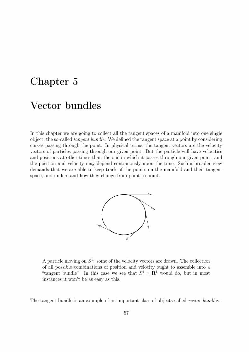
In this chapter we are going to collect all the tangent spaces of a manifold into one singleobject, the so-called tangent bundle. We defined the tangent space at a point by consideringcurves passing through the point. In physical terms, the tangent vectors are the velocityvectors of particles passing through our given point. But the particle will have velocitiesand positions at other times than the one in which it passes through our given point, andthe position and velocity may depend continuously upon the time. Such a broader viewdemands that we are able to keep track of the points on the manifold and their tangentspace, and understand how they change from point to point.

A particle moving on S1: some of the velocity vectors are drawn. The collectionof all possible combinations of position and velocity ought to assemble into a“tangent bundle”. In this case we see that S1 × R

1 would do, but in mostinstances it won’t be as easy as this.

The tangent bundle is an example of an important class of objects called vector bundles.

57

58 CHAPTER 5. VECTOR BUNDLES

5.1 Topological vector bundles

Loosely speaking, a vector bundle is a collection of vector spaces parameterized in a locallycontrollable fashion by some space.

vector spaces

topologicalspace

A vector bundle is a topological space to which a vector space is stuck at each point,

and everything fitted continuously together.

The easiest example is simply the product X × Rn, and we will have this as our localmodel.

The product of a space and an euclidean space is the local model for vector bundles.

The cylinder S1 ×R is an example.

5.1. TOPOLOGICAL VECTOR BUNDLES 59

Definition 5.1.1 An n-dimensional (real topological) vector bundle is a surjective contin-uous map

E

π

yX

such that for every p ∈ X

— the fiberπ−1(p)

has the structure of a real n-dimensional vector space

— there is an open set U ⊆ X containing p

— a homeomorphismh : π−1(U)→ U ×R

n

such that

π−1(U)h //

π|π−1(U) ##G

GGGG

GGGG

U ×Rn

prU{{ww

wwww

wwww

U

commutes, and such that for every q ∈ U the composite

hq : π−1(q)

h|π−1(q)−−−−−→ {q} ×R

n (q,t)7→t−−−−→ Rn

is a vector space isomorphism.

Example 5.1.2 The “unbounded Möbius band” given by

E = (R× [0, 1])/((p, 0) ∼ (−p, 1))

defines a 1-dimensional vector bundle by projecting onto the central circle E → [0, 1]/(0 ∼1) ∼= S1.


Restricting to an interval on the circle, we clearly see that it is homeomorphic to theproduct:

This bundle is often referred to as the canonical line bundle over S1, and is written η1 → S1.

Definition 5.1.3 Given an n-dimensional topological vector bundle π : E → X, we call

Eq = π−1(q) the fiber over q ∈ X,

E the total space and

X the base space of the vector bundle.

The existence of the (h, U)s is referred to as the local trivialization of the bundle (“thebundle is locally trivial ”), and the (h, U)s are called bundle charts. A bundle atlas is acollection B of bundle charts such that

X =⋃

(h,U)∈B

U

(B “covers” X).

Note 5.1.4 Note the correspondence the definition spells out between h and hq: for r ∈π−1(U) we have

h(r) = (π(r), hπ(r)(r))

It is (bad taste, but) not uncommon to write just E when referring to the vector bundleE → X.

Example 5.1.5 Given a topological space X, the projection onto the first factor

X ×Rn

prX

yX

is an n-dimensional topological vector bundle.

5.1. TOPOLOGICAL VECTOR BUNDLES 61

This example is so totally uninteresting that we call it the trivial bundle over X (or moredescriptively, the product bundle). More generally, any vector bundle π : E → X with abundle chart (h,X) is called trivial.

We have to specify the maps connecting the vector bundles. They come in two types,according to whether we allow the base space to change. The more general is:

Definition 5.1.6 A bundle morphism from one bundle π : E → X to another π ′ : E ′ → X ′

is a pair of maps

f : X → X ′ and f : E → E ′

such that

Ef−−−→ E ′

π

y π′

y

Xf−−−→ X ′

commutes, and such that

f |π−1(p) : π−1(p)→ (π′)−1(f(p))

is a linear map.

Definition 5.1.7 Let π : E → X be a vector bundle. A section to π is a continuous mapσ : X → E such that πσ(p) = p for all p ∈ X.

zero section

X

E

image of a section

image of the

Example 5.1.8 Every vector bundle π : E → X has a section, namely the zero section,which is the map σ0 : X → E that sends p ∈ X to zero in the vector space π−1(p). Asfor any section, the map onto its image X → σ0(X) is a homeomorphism, and we willoccasionally not distinguish between X and σ0(X) (we already did this when we talkedinformally about the unbounded Möbius band).


Example 5.1.9 The trivial bundle X ×Rn → X has

nonvanishing sections (i.e. a section whose image doesnot intersect the zero section), for instance p 7→ (p, 1)will do. The canonical line bundle η1 → S1 (the un-bounded Möbius band of example 5.1.2), however, doesnot. This follows by the intermediate value theorem:a function f : [0, 1]→ R with f(0) = −f(1) must havea zero.

1

0

The trivial bundle hasnonvanishing sections.

5.2 Transition functions

We will need to endow our bundles withsmooth structures, and in order to do thiswe will use the same trick as we used to de-fine manifolds: transport it down to an issuein Euclidean space. Given two overlappingbundle charts (h, U) and (g, V ), restricting toπ−1(U ∩ V ) both define homeomorphisms

π−1(U ∩ V )→ (U ∩ V )×Rn

which we may compose to give homeomor-phisms of (U ∩ V ) × R

n with itself. If thebase space is a smooth manifold, we may askwhether this map is smooth.

Two bundle charts. Restricting totheir intersection, how do the twohomeomorphisms to (U ∩V )×R

n

compare?

We need some names to talk about this construction.

Definition 5.2.1 Let π : E → X be an n-dimensional topological vector bundle, and letB be a bundle atlas. If (h, U), (g, V ) ∈ B then

gh−1|(U∩V )×Rn : (U ∩ V )×Rn → (U ∩ V )×R

n

are called the bundle chart transformations. The restrictions to each fiber

gqh−1q : R

n → Rn

are are linear isomorphisms (i.e. elements in GLn(R)) and the associated function

U ∩ V →GLn(R)

q 7→gqh−1q

are called transition functions.

5.3. SMOOTH VECTOR BUNDLES 63

Again, visually bundle chart transformations are given by going up and down in

π−1(U ∩ V )h|

π−1(U∩V )

vvmmmmmmmmmmmm g|π−1(U∩V )

((QQQQQQQQQQQQ

(U ∩ V )×Rn (U ∩ V )×R

n

Lemma 5.2.2 Let W be a topological space, and f : W → Mm×n(R) a continuous func-tion. Then the associated function

f∗ : W ×Rn →R

m

(w, v) 7→f(w) · v

is continuous iff f is. If W is a smooth manifold, then f∗ is smooth iff f is.

Proof: Note that f∗ is the composite

W ×Rn f×id−−−→ Mm×n(R)×R

n e−−−→ Rm

where e(A, v) = A · v. Since e is smooth, it follows that if f is continuous or smooth, thenso is f∗.

Conversely, considered as a matrix, we have that

[f(w)] = [f∗(w, e1), . . . , f∗(w, en)]

If f∗ is continuous (or smooth), then we see that each column of [f(w)] depends continuously(or smoothly) on w, and so f is continuous (or smooth).

So, requiring the bundle chart transformations to be smooth is the same as to require thetransition functions to be smooth, and we will often take the opportunity to confuse this.

Exercise 5.2.3 Show that any vector bundle E → [0, 1] is trivial.

Exercise 5.2.4 Show that any 1-dimensional vector bundle (also called line bundle) E →S1 is either trivial, or E ∼= η1. Show the analogous statement for n-dimensional vectorbundles.

5.3 Smooth vector bundles

Definition 5.3.1 Let M be a smooth manifold, and let π : E → M be a vector bundle.A bundle atlas is said to be smooth if all the transition functions are smooth.


Note 5.3.2 Spelling the differentiability out in full detail we get the following: Let (M,A)be a smooth n-dimensional manifold, π : E → M a k-dimensional vector bundle, and B abundle atlas. Then B is smooth if for all bundle charts (h1, U1), (h2, U2) ∈ B and all charts(x1, V1), (x2, V2) ∈ A, the composites going up over and across

π−1(U)h1|π−1(U)

xxppppppppppp h2|π−1(U)

&&NNNNNNNNNNN

U ×Rk

x1|U×id��

U ×Rk

x2|U×id��

x1(U)×Rk x2(U)×R

k

is a smooth function in Rn+k, where U = U1 ∩ U2 ∩ V1 ∩ V2.

Example 5.3.3 If M is a smooth manifold, then the trivial bundle is a smooth vectorbundle in an obvious manner.

Example 5.3.4 The canonical line bundle (unbounded Möbius strip) η1 → S1 is a smoothvector bundle. As a matter of fact, the trivial bundle and the canonical line bundle arethe only one-dimensional smooth vector bundles over the circle (see example 5.2.4 for thetopological case. The smooth case needs partitions of unity, which we will cover at a laterstage, see exercise 7.2.6).

Note 5.3.5 Just as for atlases of manifolds, we have a notion of a maximal (smooth)bundle atlas, and to each smooth atlas we may associate a unique maximal one in exactlythe same way as before.

Definition 5.3.6 A smooth vector bundle is a vector bundle equipped with a maximalsmooth bundle atlas.

We will often suppress the bundle atlas from the notation, so a smooth vector bundle(π : E → M,B) will occasionally be written simply π : E → M (or even worse E), if themaximal atlas B is clear from the context.

Definition 5.3.7 A smooth vector bundle (π : E →M,B) is trivial if its (maximal smooth)atlas B contains a chart (h,M) with domain all of M .

Lemma 5.3.8 The total space E of a smooth vector bundle (π : E →M,B) has a naturalsmooth structure, and π is a smooth map.

Proof: LetM be n-dimensional with atlasA, and let π be k-dimensional. Then the diagramin 5.3.2 shows that E is a smooth (n + k)-dimensional manifold. That π is smooth is the

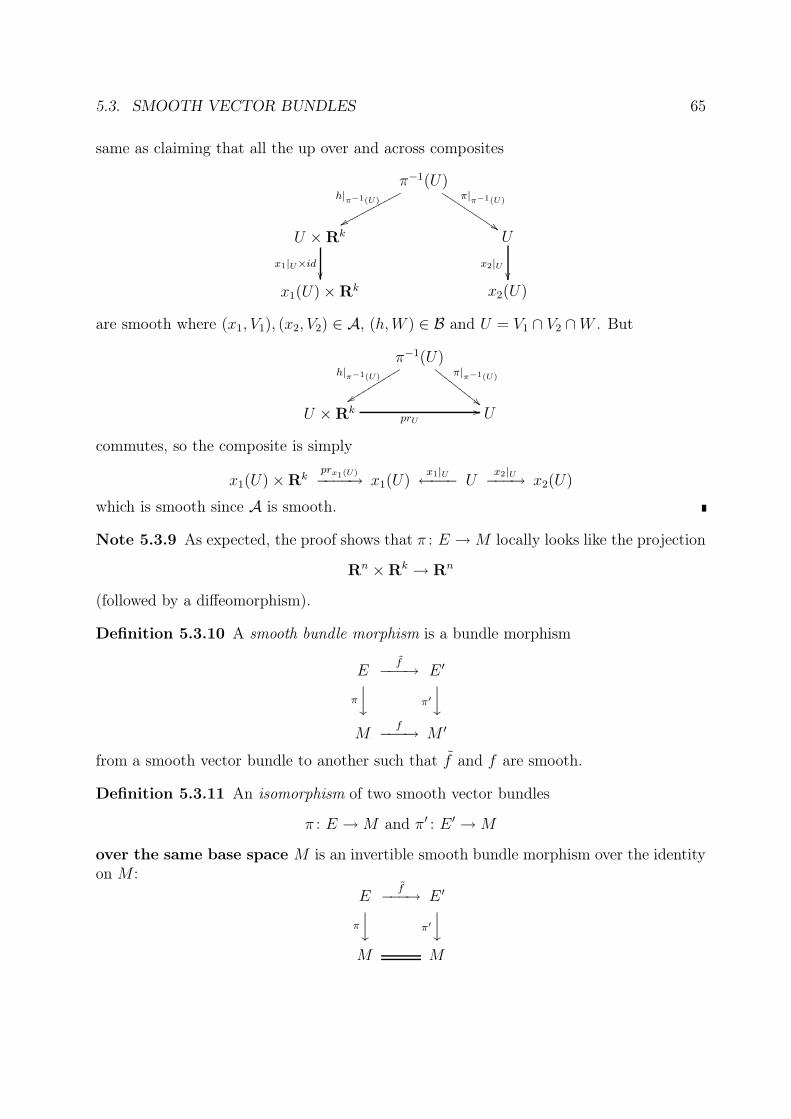
5.3. SMOOTH VECTOR BUNDLES 65

same as claiming that all the up over and across composites

π−1(U)h|

π−1(U)

xxppppppppppp π|π−1(U)

$$JJJJJJJJJJ

U ×Rk

x1|U×id��

U

x2|U��

x1(U)×Rk x2(U)

are smooth where (x1, V1), (x2, V2) ∈ A, (h,W ) ∈ B and U = V1 ∩ V2 ∩W . But

π−1(U)h|

π−1(U)

yyssssssssss π|π−1(U)

""FFF

FFFF

FF

U ×Rk

prU// U

commutes, so the composite is simply

x1(U)×Rk

prx1(U)−−−−→ x1(U)x1|U←−−− U

x2|U−−−→ x2(U)

which is smooth since A is smooth.

Note 5.3.9 As expected, the proof shows that π : E →M locally looks like the projection

Rn ×R

k → Rn

(followed by a diffeomorphism).

Definition 5.3.10 A smooth bundle morphism is a bundle morphism

Ef−−−→ E ′

π

y π′

y

Mf−−−→ M ′

from a smooth vector bundle to another such that f and f are smooth.

Definition 5.3.11 An isomorphism of two smooth vector bundles

π : E →M and π′ : E ′ →M

over the same base space M is an invertible smooth bundle morphism over the identityon M :

Ef−−−→ E ′

π

y π′

yM M


Checking whether a bundle morphism is an isomorphism reduces to checking that it is abijection:

Lemma 5.3.12 Let

Ef−−−→ E ′

π

y π′

yM M

be a smooth (or continuous) bundle morphism. If f is bijective, then it is a smooth (orcontinuous) isomorphism.

Proof: That f is bijective means that it is a bijective linear map on every fiber, or inother words: a vector space isomorphism on every fiber. Choose charts (h, U) in E and(h′, U) in E ′ around p ∈ U ⊆ M (may choose the U ’s to be the same). Then

h′fh−1 : U ×Rn → U ×R

n

is of the form (u, v) 7→ (u, αuv) where αu ∈ GLn(R) depends smoothly (or continuously)on u ∈ U . But by Cramer’s rule (αu)

−1 depends smoothly on αu, and so the inverse

(h′fh−1

)−1

: U ×Rn → U ×R

n, (u, v) 7→ (u, (αu)−1v)

is smooth (or continuous) proving that the inverse of f is smooth (or continuous).

5.4 Pre-vector bundles

A smooth or topological vector bundle is a very structured object, and much of its structureis intertwined very closely. There is a sneaky way out of having to check topologicalproperties all the time. As a matter of fact, the topology is determined by some of theother structure as soon as the claim that it is a vector bundle is made: specifying thetopology on the total space is redundant!.

5.4. PRE-VECTOR BUNDLES 67

Definition 5.4.1 A pre-vector bundle is

a set E (total space)

a topological space X (base space)

a surjective function π : E → X

a vector space structure on the fiber π−1(q) for each q ∈ X

a pre-bundle atlas B, i.e. a set of bijective functions

h : π−1(U)→ U ×Rn

with U ⊆ X open, such that

B covers X (i.e. X =⋃

(h,U)∈B U)

for every q ∈ Xhq : π

−1(q)→ Rn

is a linear isomorphism, and

the transition functions are continuous.

Definition 5.4.2 A smooth pre-vector bundle is a pre-vector bundle where the base spaceis a smooth manifold and the transition functions are smooth.

Lemma 5.4.3 Given a pre-vector bundle, there is a unique vector bundle with underlyingpre-vector bundle the given one. The same statement holds for the smooth case.


Proof: Let (π : E → X,B) be a pre-vectorbundle. We must equip E with a topologysuch that π is continuous and the bijections inthe bundle atlas are homeomorphisms. Thesmooth case follows then immediately fromthe continuous case.We must have that if (h, U) ∈ B, then π−1(U)is an open set in E (for π to be continuous).The family of open sets {π−1(U)}U⊆X open

covers E, so we only need to know what theopen subsets of π−1(U) are, but this followsby the requirement that the bijection h shouldbe a homeomorphism, That is V ⊆ π−1(U)is open if V = h−1(V ′) for some open V ′ ⊆U ×R

k. Ultimately, we get that

{h−1(V1 × V2)

∣∣∣∣ (h, U) ∈ B, V1 open in U,V2 open in R

k

}

is a basis for the topology on E.

A typical open set in π−1(U) got-ten as h−1 of the product of anopen set in U and an open set inRk

Exercise 5.4.4 Let

ηn ={([p], λp) ∈ RPn ×R

n+1 |p ∈ Sn, λ ∈ R}

Show that the projection

ηn → RPn

([p], λp) 7→ [p]

defines a non-trivial smooth vector bundle.

Exercise 5.4.5 Let p ∈ RPn and X = RPn \ {p}. Show that X is diffeomorphic to thetotal space ηn−1 of exercise 5.4.4.

5.5 The tangent bundle

We define the tangent bundle as follows:

5.5. THE TANGENT BUNDLE 69

Definition 5.5.1 Let (M,A) be a smooth n-dimensional manifold. The tangent bundleof M is defined by the following smooth pre-vector bundle

TM =∐

p∈M TpM (total space)

M (base space)

π : TM →M sends TpM to p

the pre-vector bundle atlas

BA = {(hx, U)|(x, U) ∈ A}

where hx is given by

hx : π−1(U)→U ×Rn

[γ] 7→(γ(0), (xγ)′(0))

Note 5.5.2 Since the tangent bundle is a smooth vector bundle, the total space TM is asmooth 2n-dimensional manifolds. To be explicit, its atlas is gotten from the smooth atlason M as follows.

If (x, U) is a chart on M ,

π−1(U)hx−−−→ U ×R

n x×id−−−→ x(U)×Rn

[γ]7→(xγ(0), (xγ)′(0))

is a homeomorphism to an open subset of Rn ×R

n. It is convenient to have an explicitformula for the inverse. Let (p, v) ∈ x(U)×R

n. Define the germ

γ(p, v) : (R, 0)→ (Rn, p)

by sending t (in a sufficiently small open interval containing zero) to p + tv. Then theinverse is given by sending (p, v) to

[x−1γ(p, v)] ∈ Tx−1(p)M

Lemma 5.5.3 Let f : (M,AM)→ (N,AN) be a smooth map. Then

[γ] 7→ Tf [γ] = [fγ]

defines a smooth bundle morphism

TMTf−−−→ TN

πM

y πN

y

Mf−−−→ N


Proof: Since Tf |π−1(p) = Tpf we have linearity on the fibers, and we are left with showingthat Tf is a smooth map. Let (x, U) ∈ AM and (y, V ) ∈ AN . We have to show that up,across and down in

π−1M (W )

Tf |−−−→ π−1N (V )

hx|W

y hy

yW ×R

m V ×Rn

x|W×id

y y×id

yx(W )×R

m y(V )×Rn

is smooth, where W = U ∩ f−1(V ) and Tf | is Tf restricted to π−1M (W ). This composite

sends (p, v) ∈ x(W )×Rm to [x−1γ(p, v)] ∈ π−1

M (W ) to [fx−1γ(p, v)] ∈ π−1N (V ) and finally

to (yfx−1γ(p, v)(0), (yfx−1γ(p, v))′(0) ∈ y(V )×Rn which is equal to

(yfx−1(p), D(yfx−1)(p) · v)

by the chain rule. Since yfx−1 is a smooth function, this is a smooth function too.

Lemma 5.5.4 If f : M → N and g : N → L are smooth, then

TgTf = T (gf)

Proof: It is the chain rule (made pleasant since the notation does not have to tell youwhere you are at all the time).

Note 5.5.5 The tangent space of Rn is trivial, since the identity chart induces a bundle

chart

hid : TRn →R

n ×Rn

[γ] 7→(γ(0), γ′(0))

Definition 5.5.6 A manifold is often said to be parallelizable if its tangent bundle istrivial.

Example 5.5.7 The circle is parallelizable. This is so since the map

S1 × T1S1 → TS1

(eiθ, [γ]) 7→ [eiθ · γ]

is a diffeomorphism (here (eiθ · γ)(t) = eiθ · γ(t)).

Exercise 5.5.8 The tree-sphere S3 is parallelizable


Exercise 5.5.9 All Lie groups are parallelizable. (A Lie group is a manifold with a smoothassociative multiplication, with a unit and all inverses: skip this exercise if this sounds tooalien to you).

Example 5.5.10 Let

E = {(p, v) ∈ Rn+1 ×R

n+1 | |p| = 1, p · v = 0}

Then

TSn →E[γ] 7→(γ(0), γ′(0))

is a homeomorphism. The inverse sends (p, v) ∈ E to the equivalence class of the germassociated to

t 7→ p+ tv

|p+ tv|

. pv

|p|=1

p v=0

A point in the tangent space of S2

may be represented by a unit vec-tor p together with an arbitraryvector v perpendicular to p.

–1

0

1

x

–1 –0.5 0 0.51y

–1

–0.5

0

0.5

1

z

We can’t draw all the tangentplanes simultaneously to illus-trate the tangent space of S2. Thedescription we give is in R

6.

More generally we have the following fact:

Lemma 5.5.11 Let f : M → N be an imbedding. Then Tf : TM → TN is an imbedding.

Proof: We may assume that f is the inclusion of a submanifold (the diffeomorphism partis taken care of by the chain rule which implies that Tf is a diffeomorphism if f is). Lety : V → V ′ be a chart on N such that y(V ∩ M) = V ′ ∩ (Rm × {0}). Since curves inRm × {0} have derivatives in R

m × {0} we see that

(y × id)hy(Tf(π−1M (W ∩M)) = (V ′ ∩ (Rm × {0}))×R

m × {0}⊆ R

m ×Rk ×R

m ×Rk


and by permuting the coordinates we have that Tf is the inclusion of a submanifold.

Corollary 5.5.12 If M ⊆ RN is the inclusion of a smooth submanifold of an Euclidean

space, then

TM ∼={

(p, v) ∈M×RN

∣∣∣∣v = γ′(0)

for some germ γ : (R, 0)→ (M, p)

}

(the derivation of γ happens in RN)

Exercise 5.5.13 There is an even groovier description of TSn: prove that

E =

{(z0, . . . , zn) ∈ C

n+1|n∑

i=0

z2 = 1

}

is the total space in a bundle isomorphic to TSn.

Definition 5.5.14 Let M be a smooth manifold. A vector field on M is a section in thetangent bundle.

Example 5.5.15 The circle has nonvanishing vector fields. Let [γ] 6= 0 ∈ T1S1, then

S1 → TS1, eiθ 7→ [eiθ · γ]

is a vector field (since eiθ · γ(0) = eiθ · 1) and does not intersect the zero section since(viewed as a vector in C)

|(eiθ · γ)′(0)| = |eiθ · γ′(0)| = |γ′(0)| 6= 0

The vector field spins around the circle with constant speed.

This is the same construction we used to show that S1 was parallelizable. This is a generalargument: an n dimensional manifold with n linearly independent vector fields has a trivialtangent bundle, and conversely.


Exercise 5.5.16 Construct three vector fields on S3 that are linearly independent in alltangent spaces.

Exercise 5.5.17 Prove that T (M ×N) ∼= TM × TN .

Example 5.5.18 We have just seen that S1 and S3 (if you did the exercise) both havenonvanishing vector fields. It is a hard fact that S2 does not: “you can’t comb the hair ona sphere”.

This has the practical consequence that when you want to confine the plasma in a fusionreactor by means of magnetic fields, you can’t choose to let the plasma be in the interior ofa sphere (or anything homeomorphic to it). At each point on the surface, the componentof the magnetic field parallel to the surface must be nonzero, or the plasma will leak out(if you remember your physics, there once was a formula saying something like F = qv×Bwhere q is the charge of the particle, v its velocity and B the magnetic field: hence anyparticle moving nonparallel to the magnetic field will be deflected).

This problem is solved by letting the plasma stay inside a torus S1 × S1 which does havenonvanishing vector fields (since S1 has and T (S1×S1) ∼= TS1×TS1 by the above exercise).

Although there are no nonvanishing vector fields on S2, there are certainly interesting onesthat have a few zeros. For instance “rotation around an axis” will give you a vector fieldwith only two zeros. The “magnetic dipole” defines a vector field on S2 with just one zero.

–1

–0.5

0.5

1

y

–1 –0.5 0.5 1x

A magnetic dipole on S2, seen by stereographic projection in a neighbourhoodof the only zero.

Chapter 6

Submanifolds

In this chapter we will give several important results regarding submanifolds. This willserve a twofold purpose. First of all we will acquire a powerful tool for constructing newmanifolds as inverse images of smooth functions. Secondly we will clear up the somewhatmysterious definition of submanifolds. These results are consequences of the rank theorem,which says roughly that smooth maps are – locally around “most” points – like linearprojections or inclusions of Euclidean spaces.

6.1 The rank

Definition 6.1.1 Let f : (M, p)→ (N, f(p)) be a smooth germ. The rank rkpf of f at pis the rank of the linear map Tpf . We say that a germ f has constant rank r if it has arepresentative f : Uf → N whose rank rkTqf = r for all q ∈ Uf . We say that a germ f hasrank ≥ r if it has a representative f : Uf → N whose rank rkTqf ≥ r for all q ∈ Uf .

Lemma 6.1.2 Let f : (M, p)→ (N, f(p)) be a smooth germ. If rkpf = r then there existsa neighborhood of p such that rkqf ≥ r for all q ∈ U .

Proof: Strategy: choose charts x and y, and use that the rank of the Jacobi matrix

[Dj(priyfx−1)(x(q))]

does not decrease locally. This is true since the Jacobi matrix at x(p) must contain an r×rsubmatrix which has determinant different from zero. But since the determinant functionis continuous, there must be a neighborhood around x(p) for which the determinant of ther×r submatrix stays nonzero, and hence the rank of the Jacobi matrix is at least r.

Note 6.1.3 As a matter of fact, we have shown that the subspace M rn(R) ⊆ Mn(R) of

rank r n×n matrices is a submanifold of codimension (n−r)2. Perturbing a rank r matrixmay kick you out of this manifold and into one of higher rank.

75

76 CHAPTER 6. SUBMANIFOLDS

Example 6.1.4 The map f : R→ R given by f(p) = p2 has Df(p) = 2p, and so

rkpf =

{0 p = 0

1 p 6= 0

Example 6.1.5 Consider the determinant det : M2(R)→ R with

det = a11a22 − a12a21, for A =

[a11 a12

a21 a22

]

Using the chart x : M2(R)→ R4 with

x(A) =

a11

a12

a21

a22

(and the identity chart on R) we have that

[D(det x−1)(x(A))] = [a22,−a21,−a12, a11]

(check this!) Thus we see that

rkAdet =

{0 A = 0

1 A 6= 0

By a bit of work we may prove this result also for det : Mn(R)→ R for all n.

Definition 6.1.6 Let f : M → N be a smooth map where N is n-dimensional. A pointp ∈ M is regular if Tpf is surjective (i.e. if rkpf = n). A point q ∈ N is a regular value ifall p ∈ f−1(q) are regular points. Synonyms for “non-regular” are critical or singular.

Note that a point q which is not in the image of f is a regular value since f−1(q) = ∅.

Note 6.1.7 We shall later see that these names are well chosen: the regular values are themost common ones (Sard’s theorem states this precisely, see theorem 6.6.1), whereas thecritical values are critical in the sense that they exhibit bad behavior. The inverse imagef−1(q) ⊆ M of a regular value q will turn out to be a submanifold, whereas inverse imagesof critical points usually are not.

Example 6.1.8 The names correspond to the normal usage in multi-variable calculus.

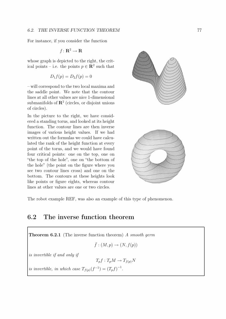
6.2. THE INVERSE FUNCTION THEOREM 77

For instance, if you consider the function

f : R2 → R

whose graph is depicted to the right, the crit-ical points – i.e. the points p ∈ R

2 such that

D1f(p) = D2f(p) = 0

– will correspond to the two local maxima andthe saddle point. We note that the contourlines at all other values are nice 1-dimensionalsubmanifolds of R

2 (circles, or disjoint unionsof circles).

In the picture to the right, we have consid-ered a standing torus, and looked at its heightfunction. The contour lines are then inverseimages of various height values. If we hadwritten out the formulas we could have calcu-lated the rank of the height function at everypoint of the torus, and we would have foundfour critical points: one on the top, one on“the top of the hole”, one on “the bottom ofthe hole” (the point on the figure where yousee two contour lines cross) and one on thebottom. The contours at these heights looklike points or figure eights, whereas contourlines at other values are one or two circles.

The robot example REF, was also an example of this type of phenomenon.

6.2 The inverse function theorem

Theorem 6.2.1 (The inverse function theorem) A smooth germ

f : (M, p)→ (N, f(p))

is invertible if and only ifTpf : TpM → Tf(p)N

is invertible, in which case Tf(p)(f−1) = (Tpf)−1.


Proof: Choose charts (x, U) and (y, V ) with p ∈ U and f(p) ∈ V . In the bases

∂

∂xi

∣∣∣∣p

, and∂

∂yj

∣∣∣∣f(p)

Tpf is given by the Jacobi matrix

[D(yfx−1)(x(p))] = [Dj(priyfx−1(x(p))]

so Tpf is invertible iff [D(yfx−1)(x(p))] is invertible. By the inverse function theorem 11.2.1in the flat case, this is the case iff yfx−1 is invertible in a neighborhood of x(p). As x andy are diffeomorphisms, this is the same as saying that f is invertible in a neighborhoodaround p.

Corollary 6.2.2 Let f : M → N be a smooth map between smooth n-manifolds. Then fis a diffeomorphism iff it is bijective and Tpf is of rank n for all p ∈M .

Proof: Since f is bijective it has an inverse function. A function has at most one inversefunction (!) so the smooth inverse functions existing locally by the inverse function theorem,must be equal to the globally defined inverse function which hence is smooth.

Exercise 6.2.3 Let G be a Lie group (a manifold with a smooth associative multiplication,with a unit and all inverses).

Show that

G→Gg 7→g−1

is smooth (some authors have this as a part of the definition, which is totally redundant).

6.3 The rank theorem

The rank theorem says that if the rank of a smooth map f : M → N is constant in aneighborhood of a point, then there are charts so that f looks like a a composite R

m →Rr ⊆ R

n, where the first map is the projection onto the first r < m coordinate directions,and the last one is the inclusion of the first r < n coordinates. So for instance, a map ofrank 1 between 2-manifolds looks locally like

R2 → R

2, (q1, q2) 7→ (q1, 0)

6.3. THE RANK THEOREM 79

Lemma 6.3.1 (The rank theorem) Let f : (M, p) → (N, f(p)) be a germ of rank ≥ r.Then there exist a chart germs

x : (M, p)→ (Rm, x(p)) and y : (N, f(p))→ (Rn, yf(p))

such thatprjyfx

−1(q) = qj for j = 1, . . . r

for all q = (q1, . . . , qm) sufficiently close to x(p). Furthermore, given any chart y we canachieve this by a choice of x, and permuting the coordinates in y.If f has constant rank r, then there exist chart germs


such thatyfx−1(q) = (q1, . . . , qr, 0, . . . , 0)

for all q = (q1, . . . , qm) sufficiently close to x(p).

Proof: If we start with arbitrary charts, we will fix them up so that we have the theorem.Hence we may just as well assume that (M, p) = (Rm, 0) and (N, f(p)) = (Rn, 0), thatf : (Rm, 0) → (Rn, 0) is a representative of the germ (if the representative you first chosewas not defined everywhere, restrict to a small ball close to zero, and use a chart to defineit on all of R

m), and that the Jacobian Df(0) has the form

Df(0) =

[A BC D

]

where A is an invertible r × r matrix (here we have used that we could permute thecoordinates).

Let fi = prif , and define x : (Rm, 0)→ (Rm, 0) by

x(t) = (f1(t), . . . , fr(t), tr+1, . . . , tm)

(where tj = prj(t)). Then

Dx(0) =

[A B0 I

]

and so detDx(0) = det(A) 6= 0. By the inverse function theorem, x is an invertible germwith inverse x−1. Choose a representative for x−1 which we by a slight abuse of notationwill call x−1. Since for sufficiently small t ∈M = R

m we have

(f1(t), . . . , fn(t)) = f(t) = fx−1x(t) = fx−1(f1(t), . . . , fr(t), tr+1, . . . , tm)

we see thatfx−1(q) = (q1, . . . , qr, fr+1x

−1(q), . . . , fnx−1(q))


and we have proven the first part of the rank theorem.

For the second half, assume rkDf(q) = r for all q. Since x is invertible

D(fx−1)(q) = Df(x−1(q))D(x−1)(q)

also has rank r for all q in the domain of definition. Note that

D(fx−1)(q) =

I 0. . . . . . . . . . . . . . . . . . . . . .[Dj(fix

−1)(q)] i=r+1,...,nj=1,...m

so since the rank is exactly r we must have that the lower right hand (n−r)×(m−r)-matrix

[Dj(fix

−1)(q)]r+1 ≤ i ≤ nr+1 ≤ j ≤ m

is the zero matrix (which says that “fix−1 does not depend on the last m− r coordinates

for i > r”). Define y : (Rn, 0)→ (Rn, 0) by setting

y(q) =(q1, . . . , qr, qr+1 − fr+1x

−1(q), . . . , qn − fnx−1(q))

where q = (q1, . . . , qr, 0, . . . , 0). Then

Dy(q) =

[I 0? I

]

so y is invertible and yfx−1 is represented by

q = (q1, . . . , qm) 7→(q1, . . . , qr, fr+1x

−1(q)− fr+1x−1(q), . . . , fnx

−1(q)− fnx−1(q))

=(q1, . . . , qr, 0, . . . , 0)

where the last equation holds since Dj(fix−1)(q) = 0 for r < i ≤ n and r < j ≤ m so

. . . , fnx−1(q)− fnx−1(q) = 0 for r < i ≤ n for q close to the origin.

The proof of the rank theorem has the following corollary. It treats the case when the rankis maximal (and hence constant). Note that the permutations have been removed from thefirst part. Also note that if f : M → N has rank dim(N), then dim(N) ≤ dim(M) and iff has rank dim(M) then dim(M) ≤ dim(N).

Corollary 6.3.2 Let M and N be smooth manifolds of dimension dim(M) = m anddim(N) = n.

Let f : (M, p)→ (N, f(p)) be a germ of rank n. Then there exist a chart germ

x : (M, p)→ (Rm, x(p))

6.4. REGULAR VALUES 81

such that for any chart germ

y : (N, f(p))→ (Rn, yf(p))

yfx−1(q) = (q1, . . . , qn)

for all q = (q1, . . . , qm) sufficiently close to x(p).

If f has rank m, then there exist chart germs


such that

yfx−1(q) = (q1, . . . , qm, 0, . . . , 0)

for all q = (q1, . . . , q(dim(M)) sufficiently close to x(p).

Exercise 6.3.3 Let f : M →M be smooth such that f ◦ f = f and M connected. Provethat f(M) ⊆ M is a submanifold. If you like point-set topology, prove that f(M) ⊆M isclosed.

6.4 Regular values

Since the rank can only increase locally, there are certain situations where constant rankis guaranteed, namely when the rank is maximal.

Definition 6.4.1 A smooth map f : M → N is

a submersion if rkTpf = dimN (that is Tpf is surjective)

an immersion if rkTpf = dimM (Tpf is injective)

for all p ∈M .

Note 6.4.2 To say that a map f : M → N is a submersion is equivalent to claiming thatall points p ∈ M are regular (Tpf is surjective), which again is equivalent to claiming thatall q ∈ N are regular values (values that are not hit are regular by definition).


Theorem 6.4.3 Letf : M → N

be a smooth map where M is n+ k-dimensional and N is n-dimensional. If q = f(p) is aregular value, then

f−1(q) ⊆ M

is a k-dimensional smooth submanifold.

Proof: We must display a chart (x,W ) such that x(W ∩ f−1(q)) = x(W ) ∩ (Rk × {0}).Since p is regular, the rank of f must be n in a neighborhood of p, so by the rank theorem6.3.1, there are charts (x, U) and (y, V ) around p and q such that x(p) = 0, y(q) = 0 and

yfx−1(t1, . . . , tn+k) = (t1, . . . , tn), for t ∈ x(U ∩ f−1(V ))

Let W = U ∩ f−1(V ), and note that f−1(q) = (yf)−1(0). Then

x(W ∩ f−1(q)) =x(W ) ∩(yfx−1

)−1(0)

={(0, . . . , 0, tn+1, . . . , tn+k) ∈ x(W )}=({0} ×R

k) ∩ x(W )

and so (permuting the coordinates) f−1(q) ⊆M is a k-dimensional submanifold as claimed.

Exercise 6.4.4 Give a new proof which shows that Sn ⊂ Rn+1 is a smooth submanifold.

Note 6.4.5 Not all submanifolds can be realized as the inverse image of a regular value ofsome map (e.g. the zero section in the canonical line bundle η1 → S1 can not, see 6.4.24),but the theorem still gives a rich source of important examples of submanifolds.

Example 6.4.6 The example 6.1.8 gives two examples illustrating the theorem. The robotexample is another example. In that example we considered a function

f : S1 × S1 → R1

and found three critical values.

To be more precise:f(eiθ, eiφ) = |3− eiθ − eiφ|

and so (using charts corresponding to the angles: conveniently all charts give the sameformulas in this example) the Jacobi matrix at (eiθ, eiφ) equals

1

f(eiθ, eiφ)[3 sin θ − cos φ sin θ + sinφ cos θ, 3 sinφ− cos θ sinφ+ sin θ cosφ]


(exercise: do this). The rank is one, unless both coordinates are zero, in which case we getthat we must have sin θ = sin φ = 0, which leaves the points

(1, 1), (−1,−1), (1,−1), and (−1, 1)

giving the critical values 1, 5 and (twice) 3.

Exercise 6.4.7 Fill out the details in the robot example. Then do it in three dimensions.

Example 6.4.8 Consider the special linear group

SLn(R) = {A ∈ GLn(R) | det(A) = 1}

We show that SL2(R) is a 3-dimensional manifold. The determinant function is given by

det : M2(R)→ R

A =

[a11 a12

a21 a22

]7→ det(A) = a11a22 − a12a21

and so with the obvious coordinates M2(R) ∼= R4 (sending A to [a11 a12 a21 a22]

t) we havethat

D(det)(A) =[a22 −a21 −a12 a11

]

Hence the determinant function has rank 1 at all matrices, except the zero matrix, and inparticular 1 is a regular value.

Exercise 6.4.9 Show that SL2(R) is diffeomorphic to S1 ×R2.

Exercise 6.4.10 If you have the energy, you may prove that SLn(R) is an (n2 − 1)-dimensional manifold.

Example 6.4.11 The subgroup O(n) ⊆ GLn(R) of orthogonal matrices is a submanifold

of dimension n(n−1)2

.

To see this, recall that A ∈ GLn(R) is orthogonal iff AtA = I. Note that AtA is alwayssymmetric. The space Sym(n) of all symmetric matrices is diffeomorphic to R

n(n+1)/2 (theentries on and above the diagonal are arbitrary). We define a map

f : GLn(R)→Sym(n)

A 7→AtA

which is smooth (since matrix multiplication and transposition is smooth), and such that

O(n) = f−1(I)

We must show that I is a regular value, and we offer two proofs, one computional usingthe Jacobi matrix, and one showing more directly that TAf is surjective for all A ∈ O(n).


We present both proofs, the first one since it is very concrete, and the second one since itis short and easy to follow.

First the Jacobian argument. We use the usual chart on GLn(R) ⊆ Mn(R) ∼= Rn2

bylisting the entries in lexicographical order, and the chart pr : Sym(n) ∼= R

n(n+1)/2 withprkl[aij] = akl (also in lexicographical order) only defined for 1 ≤ i ≤ j ≤ n. Thenprk<lf([aij]) =

∑nk+1 aikajk, and a straight forward calculation yields that if A = [aij] then

Dklpri<jf(A) =

ajl k = i < j

ail i < j = k

2ail i = j = k

0 otherwise

In particular

Dklpri<jf(I) =

1 k = i < j = l

1 l = i < j = k

2 i = j = k = l

0 otherwise

and rkDf(I) = n(n + 1)/2 since Df(I) is on echelon form, with no vanishing rows (ex.for n = 2 and n = 3 the Jacobi matrices are

21 1

2

, and

21 1

1 12

1 12

(in the first matrix the colums are the partial derivatives in the 11, 12, 21 and 22-variable,and the rows are the projection on the 11 12 and 22-factor. Likewise in the second one)).

For any A ∈ GLn(R) we define the diffeomorphism

LA : GLn(R)→ GLn(R)

by LA(B) = A ·B. Note that if A ∈ O(n) then

f(LA(B)) = f(AB) = (AB)tAB = BtAtAB = BtB = f(B)

and so by the chain rule and the fact that D(LA)(B) = A we get that

Df(I) = D(fLA)(I) = D(f)(LAI)D(LA)(I) = D(f)(A)A

implying that rkD(f)(A) = n(n + 1)/2 for all A ∈ O(n). This means that A is a regularpoint for all A ∈ O(n) = f−1(I), and so I is a regular value, and O(n) is an

n2 − n(n + 1)/2 = n(n− 1)/2


dimensional submanifold.

For the other proof of the fact that I is a regular value, notice that all tangent vectors inTAGLn(R) = TAMn(R) are in the equivalence class of a linear curve

νB(s) = A+ sB, B ∈Mn(R), s ∈ R

We have that

fνB(s) = (A+ sB)t(A + sB) = AtA+ s(AtB +BtA) + s2BtB

and so

TAf [νB] = [fνB] = [γB]

where γB(s) = AtA+ s(AtB +BtA). Similarly, all tangent vectors in TISym(n) are in theequivalence class of a linear curve

αC(s) = I + sC

for C a symmetric matrix. If A is orthogonal, we see that γ 12AC = αC , and so TAf [ν 1

2AC ] =

[αC ], and TAf is surjective. Since this is true for all A ∈ O(n) we get that I is a regularvalue.

Exercise 6.4.12 Consider the inclusion O(n) ⊆ Mn(R), giving a description of the tan-gent bundle og O(n) along the lines of corollary 5.5.12. Show that under the isomorphism

TMn(R) ∼= Mn(R)×Mn(R), [γ] � (γ(0), γ′(0))

the tangent bundle of O(n) corresponds to the projection on the first factor

E = {(g, A) ∈ O(n)×Mn(R)|At = −gtAgt} → O(n).

This also shows that O(n) is parallelizable, since we get an obvious bundle isomorphisminduced by

E → O(n)× {B ∈ Mn(R)|Bt = −Bt}, (g, A) 7→ (g, g−1A)

(a matrix B satisfying Bt = −Bt is called a skew matrix).

Note 6.4.13 The multiplication

O(n)×O(n)→ O(n)

is smooth (since multiplication of matrices is smooth in Mn(R) ∼= Rn2

, and 3.5.14), andso O(n) is a Lie group. The same of course applies to SLn(R).


Exercise 6.4.14 Prove that

C→M2(R)

x+ iy 7→[x −yy x

]

defines an imbedding. More generally it defines an imbedding

Mn(C)→Mn(M2(R)) ∼= M2n(R)

Show also that this imbedding sends “conjugate transpose” to “transpose” and “multiplica-tion” to “multiplication”.

Exercise 6.4.15 Prove that the unitary group

U(n) = {A ∈ GLn(C)|AtA = I}is a Lie group of dimension n2.

Exercise 6.4.16 Prove that O(n) is compact and has two connected components. Thecomponent consisting of matrices of determinant 1 is called SO(n), the special orthogonalgroup.

Note 6.4.17 SO(2) is diffeomorphic to S1 (prove this), and SO(3) is diffeomorphic to thereal projective 3-space (don’t prove that).

Note 6.4.18 It is a beautiful fact that if G is a Lie group (e.g. GLn(R)) and H ⊆ Gis a closed subset containing the identity, and which is closed under multiplication, thenH ⊆ G is a “Lie subgroup”. We will not prove this fact, (see e.g. Spivak’s book I, theorem10.15), but note that it implies that all matrix groups such as O(n) are Lie groups sinceGLn(R) is.

Exercise 6.4.19 A k-frame in Rn is a k-tuple of orthonormal vectors in R

n. Define aStiefeld manifold V k

n as the subset

V kn = {k-frames in R

n}

of Rnk. Show that V k

n is a compact smooth nk − k(k+1)2

-dimensional manifold.

Note 6.4.20 In the literature you will often find a different definition, where a k-frameis just a k-tuple of linearly independent vectors. Then the Stiefeld manifold is an opensubset of the Mn×k(R), and so is clearly a smooth manifold – but this time of dimensionnk.

A k-frame defines a k-dimensional linear subspace of Rn. The Grassmann manifold Gk

n

have as underlying set the set of k-dimensional linear subspaces of Rn, and is topologized

as the quotient space of the Stiefeld manifold. The Grassmann manifolds are importantsince they classify vector bundles.


Exercise 6.4.21 Let Pn be the space of degree n polynomials. Show that the space ofsolutions to the equation

(y′′)2 − y′ + y(0) + xy′(0) = 0

is a 1-dimensional submanifold of P3.

Exercise 6.4.22 Make a more interesting exercise along the lines of the previous, andsolve it.

Exercise 6.4.23 Let A ∈Mn(R) be a symmetric matrix. For what values of a ∈ R is thequadric

MAa = {p ∈ R

n | ptAp = a}an n− 1-dimensional smooth manifold?

Exercise 6.4.24 Consider the canonical line bundle

η1 → S1

Prove that there is no smooth map f : η1 → R such that the zero section is the inverseimage of a regular value of f .

More generally, show that there is no map f : η1 → N for any manifold N such that thezero section is the inverse image of a regular value of f .

Exercise 6.4.25 In a chemistry book I found van der Waal’s equation, which gives a rela-tionship between the temperature T , the pressure p and the volume V , which supposedlyis somewhat more accurate than the ideal gas law pV = nRT (n is the number of moles ofgas, R is a constant). Given the relevant positive constants a and b, prove that the set ofpoints (p, V, T ) ∈ (0,∞)× (nb,∞)× (0,∞) satisfying the equation

(p− n2a

V 2

)(V − nb) = nRT

is a smooth submainfold of R3.

Exercise 6.4.26 Consider the set LFn,k of labelled flexible n-gons in Rk. A labelled flexible

n-gon is what you get if you join n > 2 straight lines of unit length to a closed curve andlabel the vertices from 1 to n.

A labelled flexible 8-gon in R2.

Let n be odd and k = 2. Show that LFn,2 is a smooth submanifold of R2 × (S1)n−1 of

dimension n.

Exercise 6.4.27 Prove that the set of non-self-intersecting flexible n-gons in R2 is a

manifold.


6.5 Immersions and imbeddings

We are finally closing in on the promised “real” definition of submanifolds, or rather, ofimbeddings. The condition of being an immersion is a readily checked property, since weonly have to check the derivatives in every point. The rank theorem states that in somesense “locally” immersions are imbeddings. But how much more do we need? Obviously,an imbedding is injective.

Something more is needed, as we see from the following example

Example 6.5.1 Consider the injective smooth map

f : (0, 3π/4)→ R2

given by

f(t) = sin(2t)(cos t, sin t)

Then

Df(t) = [(1− 3 sin2 t) cos t, (3 cos2 t− 1) sin t]

is never zero and f is an immersion.

However,(0, 3π/4)→ im{f}

is not a homeomorphism where

im{f} = f((0, 3π/4)) ⊆ R2

has the subspace topology. For, if it were a homeo-morphism, then

f((π/4, 3π/4)) ⊆ im{f}

would be open (for the inverse to be continuous). Butany open ball around (0, 0) = f(π/2) in R

2 must con-tain a piece of f((0, π/4)), so f((π/4, 3π/4)) ⊆ im{f}is not open.Hence f is not an imbedding.

–0.6

–0.4

–0.2

0

0.2

0.4

0.6

0.2 0.4 0.6

The image of f is a sub-space of R

2.

Exercise 6.5.2 Let

R

∐R→ R

2

be defined by sending x in the first summand to (x, 0) and y in the second summand to(0, ey). This is an injective immersion, but not an imbedding.

6.5. IMMERSIONS AND IMBEDDINGS 89

Exercise 6.5.3 Let

R

∐S1 → C

be defined by sending x in the first summandto (1+ ex)eix and being the inclusion S1 ⊆ C

on the second summand. This is an injectiveimmersion, but not an imbedding.

–1

–0.5

0.5

1

–1 –0.5 0.5 1 1.5 2

The image is not a submanifold ofC.

But, strangely enough these examples exhibit the only thing that can go wrong: if aninjective immersion is to be an imbedding, the map to the image has got to be a homeo-morphism.

Theorem 6.5.4 Let f : M → N be an immersion such that the induced map

M → im{f}

is a homeomorphism where im{f} = f(M) ⊆ N has the subspace topology, then f is animbedding.

Proof: Let p ∈M . The rank theorem says that there are charts

x1 : U1 → U ′1 ⊆ R

n

and

y1 : V1 → V ′1 ⊆ R

n+k

with x1(p) = 0 and y1(f(p)) = 0 such that

y1fx−11 (t) = (t, 0) ∈ R

n ×Rk = R

n+k

for all t ∈ x1(U1 ∩ f−1(V1)).

Since V ′1 is open, it contains open rectangles around the origin. Choose one such rectangle

(see the picture below)

V ′2 = U ′ × B ⊆ ((U ′

1 ∩ x1f−1(V1))×R

k) ∩ V ′1 ⊆ R

n ×Rk


Let U = x−11 (U ′), x = x1|U and V2 = y−1

1 (V ′2).

Since M → f(M) is a homeomorphism, f(U) is an open subset of f(M), and since f(M)has the subspace topology, f(U) = W ∩ f(M) where W is an open subset of N (here isthe crucial point where complications as in example 6.5.1 are excluded: there are no other“branches” of f(M) showing up in W ).

Let V = V2 ∩W , V ′ = V ′2 ∩ y1(W ) and y = y1|V .

Then we see that f(M) ⊆ N is a submanifold (y(f(M)∩ V ) = yf(U) = (Rn×{0})∩ V ′),and M → f(M) is a bijective local diffeomorphism (the constructed charts show that bothf and its inverse are smooth around every point), and hence a diffeomorphism.

We note the following useful corollary:

Corollary 6.5.5 Let f : M → N be an injective immersion from a compact manifold M .Then f is an imbedding.

Proof: We only need to show that the continuous map M → f(M) is a homeomorphism.It is injective since f is, and clearly surjective. But from point set topology (theorem 10.7.8)we know that it must be a homeomorphism since M is compact and f(M) is Hausdorff(f(M) is Hausdorff since it is a subspace of the Hausdorff space N).

Exercise 6.5.6 Let a, b ∈ R, and consider the map

fa,b : R→ S1 × S1

t 7→ (eiat, eibt)

Show that fa,b is an immersion if either a or b is different from zero. Show that fa,b factorsthrough an imbedding S1 → S1 × S1 iff either b = 0 or a/b is rational.

6.6. SARD’S THEOREM 91

–3

–2

–1

0

1

2

3

–3

–2

–1

0

1

2

3

–1

0

1

Part of the picture if a/b = π (this goes on forever)

Exercise 6.5.7 Consider smooth maps

Mi−−−→ N

j−−−→ L

Show that if the composite ji is an imbedding, then i is an imbedding.

6.6 Sard’s theorem

For reference we cite Sard’s theorem, which says that regular values are the common stateof affairs (in technical language: critical values have “measure zero” while regular valuesare “dense”). Proofs can be found in many references, for instance in Milnor’s book [M].There are many verisons, but we list only the following simple form:

Theorem 6.6.1 Let f : M → N be a smooth map and U ⊆ N an open subset. Then Ucontains a regular value for f .

Chapter 7

Partition of unity

7.1 Definitions

In this chapter we define partitions of unity. They are smooth devices making it possible topatch together some types of local information into global information. They come in theform of “bump functions” such that around any given point there are only finitely many ofthem that are nonzero, and such that the sum of their values is 1.

This can be applied for instance to patch together the nice local structure of a manifold toan imbedding into an Euclidean space, construct sensible metrics on the tangent spaces (so-called Riemannian metrics), and in general to construct smooth functions with desirableproperties.

Definition 7.1.1 Let U be an open covering of a space X. We say that U is locally finiteif each p ∈ X has a neighborhood which intersects only finitely many sets in U .

Definition 7.1.2 Let X be a space. The support of a function f : X → R is the closureof the subset of X with nonzero values, i.e.

supp(f) = {x ∈ X|f(x) 6= 0}

93

94 CHAPTER 7. PARTITION OF UNITY

Definition 7.1.3 A family of continuous function

φα : X → [0, 1]

is called a partition of unity if

the collection of subsets { {p ∈ X|φα(p) 6= 0} } is a locally finite open covering of X,

for all p ∈ X the (finite) sum∑

α φα(p) = 1.

The partition of unity is said to be subordinate to a covering U of X if in addition

for every φα there is a member U of U such that supp(φα) ⊆ U .

Partitions of unity are used to patch together local structures to global ones.

Given a space that is not too big and complicated (for instance if it is a compact manifold)it may not be surprising that we can build a partition of unity on it. What is moresurprising is that on smooth manifolds we can build smooth partitions of unity (that is,all the φα’s are smooth).

In order to this we need smooth bump functions.

7.2 Smooth bump functions

Let λ : R→ R be defined by

λ(t) =

{0 for t ≤ 0

e−1/t2 for t > 0

This is a smooth function (note thatall derivatives in zero are zero: it isdefinitely not analytic) with valuesbetween zero and one.

0

0.2

0.4

0.6

0.8

1

–1 1 2 3t

Exercise 7.2.1 Prove that λ is smooth.

7.2. SMOOTH BUMP FUNCTIONS 95

For 0 < ε, let βε : R → R be givenby

βε(t) = λ(t) · λ(ε− t)For ε = 1 it looks like

0

2e–05

4e–05

6e–05

8e–05

0.0001

0.00012

0.00014

0.00016

0.00018

0.0002

0.00022

0.00024

0.00026

0.00028

0.0003

0.00032

0.00034

–1 1 2 3t

It is a small bump, but it is nonzerobetween 0 and ε, and so we may de-fine the function αε : R → R whichascends from zero to one smoothlybetween zero and ε by means of

αε(t) =

∫ x0βε(x) dx∫ ε

0βε(x) dx 0

0.2

0.4

0.6

0.8

1

–0.4 –0.2 0.2 0.4 0.6 0.8 1 1.2 1.4x

and finally the ultimate bump func-tion γ(r,ε) : R

n → R where 0 < rgiven by

γ(r,ε)(x) = 1− αε(|x| − r)

which is zero |x| ≥ r+ ε and one for|x| ≤ r.

0.2

0.4

0.6

0.8

1

–2 –1 1 2t

Example 7.2.2 Smooth bump functions are very handy, for instance if you want to joincurves in a smooth fashion (for instance if you want to design smooth highways!) Theyalso allow you to drive smoothly on a road with corners: the curve γ : R → R

2 given byγ(t) = (te−1/t2 , |te−1/t2 |) is smooth, although its image is not.


Exercise 7.2.3 Show that any function germ φ : (M, p)→ (R, φ(p)) has a smooth repre-sentative φ : M → R.

Exercise 7.2.4 Let M and N be smooth manifolds and f : M → N a continuous map.Show that f is smooth if for all smooth φ : N → R the composite φf : M → R is smooth.

Exercise 7.2.5 Show that any smooth vector bundle E → [0, 1] is trivial (smooth on theboundary means what you think it does: don’t worry).

Exercise 7.2.6 Show that any 1-dimensional smooth vector bundle (also called line bun-dle) E → S1 is either trivial, or E ∼= η1. Show the analogous statement for n-dimensionalvector bundles.

7.3 Refinements of coverings

If 0 < r let En(r) = {x ∈ Rn||x| < r} be the open n-dimensional ball of radius r centered

at the origin.

Lemma 7.3.1 Let M be an n-dimensional manifold. Then there is a countable atlas Asuch that x(U) = En(3) for all (x, U) ∈ A and such that

⋃

(x,U)∈A

x−1(En(1)) = M

If M is smooth all charts may be chosen to be smooth.

Proof: Let B be a countable basis for the topology on M . For every p ∈M there is a chart(x, U) with x(p) = 0 and x(U) = En(3). The fact that that B is a basis for the topologygives that there is a V ∈ B with

p ∈ V ⊆ x−1(En(1))

For each such V ∈ B choose just one such chart (x, U) with x(U) = En(3) and

x−1(0) ∈ V ⊆ x−1(En(1))

The set of these charts is the desired countable A.

If M were smooth we just append “smooth” in front of every “chart” in the proof above.

Lemma 7.3.2 Let M be a manifold. Then there is a sequence A1 ⊆ A2 ⊆ A3 ⊆ . . . ofcompact subsets of M such that for every i ≥ 1 the compact subset Ai is contained in theinterior of Ai+1 and such that

⋃iAi = M

7.3. REFINEMENTS OF COVERINGS 97

Proof: Let {(xi, Ui)}i=1,... be the countable atlas of the lemma above, and let

Ak =k⋃

i=1

x−1i (En(2− 1/k))

Definition 7.3.3 Let U be an open covering of a space X. We say that another cover Vis a refinement of U if every member of V is contained in a member of U .

Definition 7.3.4 Let M be a manifold and let U be an open cover of M . A good atlassubordinate to U is a countable atlas A on M such that

1) the cover {V }(x,V )∈A is a locally finite refinement of U ,

2) x(V ) = En(3) for each (x, V ) ∈ A and

3)⋃

(x,V )∈A x−1(En(1)) = M .

Theorem 7.3.5 Let M be a manifold and let U be an open cover of M . Then there existsa good atlas A subordinate to U . If M is smooth, then A may be chosen smooth too.

Proof: The remark aboutthe smooth situation willfollow by the same proof.Choose a a sequence

A1 ⊆ A2 ⊆ A3 ⊆ . . .

of compact subsets of Msuch that for every i ≥ 1the compact subset Ai iscontained in the interior ofAi+1 and such that

⋃iAi =

M .For every point

p ∈ Ai+1 − int(Ai)

choose a Up ∈ U withp ∈ Up and choose a chart(yp,Wp) such that p ∈ Wp

and yp(p) = 0.

The positioning of the charts

Since int(Ai+2)− Ai−1, yp(Wp) and Up are open there is an εp > 0 such that

En(εp) ⊆ yp(Wp), y−1p (En(εp)) ⊆ (int(Ai+2)− Ai−1) ∩ Up


Let Vp = y−1p (En(εp)) and

xp =3

εpyp|Vp

: Vp → En(3)

Then {x−1p (En(1))}p cover the compact set Ai+1 − int(Ai), and we may choose a finite set

of points p1, . . . , pk such that

{x−1pj

(En(1))}j=1,...,k

still cover Ai+1 − int(Ai).

Letting A consist of the (xpj, Vpj

) as i and j vary we have proven the theorem. �

7.4 Existence of smooth partitions of unity on smooth

manifolds.

Theorem 7.4.1 Let M be a differentiable manifold, and let U be a covering of M . Thenthere is a smooth partition of unity of M subordinate to U .

Proof: To the good atlas A = {(xi, Vi)} subordinate to U constructed in theorem 7.3.5 wemay assign functions {ψi} as follows

ψi(q) =

{γ(1,1)(xi(q)) for q ∈ Vi = x−1

i (En(3))

0 otherwise

The function ψi has support x−1i (En(2)) and is obviously smooth. Since {Vi} is locally

finite, around any point p ∈M there is an open set such there are only finitely many ψi’swith nonzero values, and hence the expression

σ(p) =∑

i

ψi(p)

defines a smooth function M → R with everywhere positive values. The partition of unityis then defined by

φi(p) = ψi(p)/σ(p)

�

7.5. IMBEDDINGS IN EUCLIDEAN SPACE 99

7.5 Application: every compact smooth manifold may

be imbedded in an Euclidean space

As an application, we will prove the easy version of Whitney’s imbedding theorem. Thehard version states that any manifold may be imbedded in the Euclidean space of thedouble dimension. We will only prove:

Theorem 7.5.1 Let M be a compact smooth manifold. Then there is an imbedding M →RN for some N .

Proof: Assume M has dimension m. Choose a finite good atlas

A = {xi, Vi}i=1,...,r

Define ψi : M → R and ki : M → Rm by

ψi(p) =

{γ(1,1)(xi(p)) for p ∈ Vi0 otherwise

ki(p) =

{ψi(p) · xi(p) for p ∈ Vi0 otherwise

Consider the map

f : M →r∏

i=1

Rm ×

r∏

i=1

R

p 7→ ((k1(p), . . . , kr(p)), (ψ1(p), . . . , ψr(p)))

We shall prove that this is an imbedding by showing that it is an immersion inducing ahomeomorphism onto its image.

Firstly, f is an immersion, because for every p ∈ M there is a j such that Tpkj has rankm.

Secondly, assume f(p) = f(q) for two points p, q ∈ M . Assume p ∈ x−1j (Em(1)). Then

we must have that q is also in x−1j (Em(1)) (since ψj(p) = ψj(q)). But then we have that

kj(p) = xj(p) is equal to kj(q) = xj(q), and hence p = q since xj is a bijection.

Since M is compact, f is injective (and so M → f(M) is bijective) and RN Hausdorff,

M → f(M) is a homeomorphism by theorem .

Techniques like this are used to construct imbeddings. However, occasionally it is importantto know when imbeddings are not possible, and then these techniques are of no use. Forinstance, why can’t we imbed RP2 in R

3? Proving this directly is probably very hard. Forsuch problems algebraic topology is needed.

Chapter 8

Constructions on vector bundles

8.1 Subbundles and restrictions

There are a variety of important constructions we need to address. The first of these havebeen lying underneath the surface for some time:

Definition 8.1.1 Let

π : E → X

be an n-dimensional vector bundle. A k-dimensional subbundle of this vector bundle isa subset E ′ ⊆ E such that around any pointthere is a bundle chart (h, U) such that

h(π−1(U) ∩ E ′) = U × (Rk × {0}) ⊆ U ×Rn

Note 8.1.2 It makes sense to call such a sub-set E ′ ⊆ E a subbundle, since we see that thebundle charts, restricted to E ′, define a vec-tor bundle structure on π|E′ : E ′ → X whichis smooth if we start out with a smooth atlas.

A one-dimensional subbundle in a

two-dimensional vector bundle: pick

out a one-dimensional linear sub-

space of every fiber in a continuous

(or smooth) manner.

Example 8.1.3 Consider the trivial bundle S1 × C → S1. The canonical line bundleη1 → RP1 ∼= S1 can be thought of as the subbundle given by

{(eiθ, teiθ/2) ∈ S1 ×C|t ∈ R} ⊆ S1 ×C.

Exercise 8.1.4 Spell out the details of the previous example. Also show that

ηn ={([p], λp) ∈ RPn ×R

n+1 |p ∈ Sn, λ ∈ R}⊆ RPn ×R

n+1

101

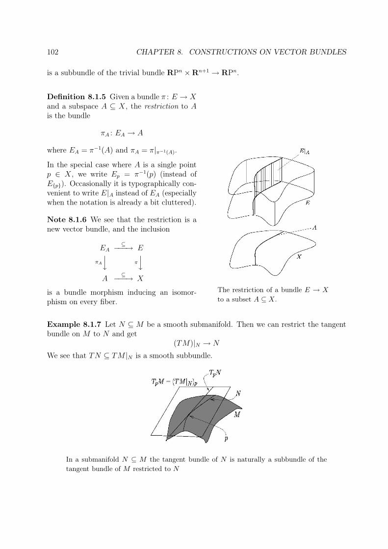
102 CHAPTER 8. CONSTRUCTIONS ON VECTOR BUNDLES

is a subbundle of the trivial bundle RPn ×Rn+1 → RPn.

Definition 8.1.5 Given a bundle π : E → Xand a subspace A ⊆ X, the restriction to Ais the bundle

πA : EA → A

where EA = π−1(A) and πA = π|π−1(A).

In the special case where A is a single pointp ∈ X, we write Ep = π−1(p) (instead ofE{p}). Occasionally it is typographically con-venient to write E|A instead of EA (especiallywhen the notation is already a bit cluttered).

Note 8.1.6 We see that the restriction is anew vector bundle, and the inclusion

EA⊆−−−→ E

πA

y π

y

A⊆−−−→ X

is a bundle morphism inducing an isomor-phism on every fiber.

The restriction of a bundle E → X

to a subset A ⊆ X.

Example 8.1.7 Let N ⊆M be a smooth submanifold. Then we can restrict the tangentbundle on M to N and get

(TM)|N → N

We see that TN ⊆ TM |N is a smooth subbundle.

In a submanifold N ⊆ M the tangent bundle of N is naturally a subbundle of the

tangent bundle of M restricted to N

8.1. SUBBUNDLES AND RESTRICTIONS 103

Definition 8.1.8 A bundle morphism

E1f−−−→ E2

π1

y π2

yX1 −−−→ X2

is said to be of constant rank r if restricted to each fiber f is a linear map of rank r.

Note that this is a generalization of our concept of constant rank of smooth maps.

Theorem 8.1.9 (Rank theorem for bundles) Consider a bundle morphism

E1f //

π1 AAA

AAAA

AE2

π2~~}}}}

}}}}

X

over a space X with constant rank r. Then around any point p ∈ X there are bundle charts(h, U) and (g, U) such that

E1|Uf |U−−−→ E2|U

h

y g

y

U ×Rm (u,(t1 ,...,tm))7→(u,(t1 ,...,tr ,0,...,0))−−−−−−−−−−−−−−−−−−−→ U ×R

n

commutes.

Furthermore if we are in a smooth situation, these bundle charts may be chosen to besmooth.

Proof: This is a local question, so translating via arbitrary bundle charts we may assumethat we are in the trivial situation

U ′ ×Rm

f //

prU′

$$III

IIII

III

U ′ ×Rn

prU′

zzuuuuuuuuu

U ′

with f(u, v) = (u, (f 1u(v), . . . , f

nu (v))), and rkfu = r. By a choice of basis on R

m and Rn

we may assume that fu is represented by a matrix

[A(u) B(u)C(u) D(u)

]


with A(p) ∈ GLr(R) and D(p) = C(p)A(p)−1B(p) (the last equation follows as the rankrkfp is r). We change the basis so that this is actually true in the standard basis.

Let p ∈ U ⊆ U ′ be the open set U = {u ∈ U ′|det(A(u)) 6= 0}. Then again D(u) =C(u)A(u)−1B(u) on U .

Leth : U ×R

m → U ×Rm, h(u, v) = (u, hu(v))

be the homeomorphism where hu is given by the matrix[A(u) B(u)

0 I

]

Letg : U ×R

n → U ×Rn, g(u, w) = (u, gu(w))

be the homeomorphism where gu is given by the matrix[

I 0−C(u)A(u)−1 I

]

Then gfh−1(u, v) = (u, (gfh−1)u(v)) where (gfh−1)u is given by the matrix

[I 0

−C(u)A(u)−1 I

] [A(u) B(u)C(u) D(u)

] [A(u) B(u)

0 I

]−1

=

[I 0

−C(u)A(u)−1 I

] [A(u) B(u)C(u) D(u)

] [A(u)−1 −A(u)−1B(u)

0 I

]

=

[I 0

−C(u)A(u)−1 I

] [I 0

C(u)A(u)−1 0

]

=

[I 00 0

]

as claimed (the right hand lower zero in the answer is really a 0 = −C(u)A(u)−1B(u) +D(u)).

Recall that if f : V → W is a linear map of vector spaces, then the kernel (or null space)is the subspace

ker{f} = {v ∈ V |f(v) = 0} ⊆ V

and the image (or range) is the subspace

im{f} = {w ∈ W |there is a v ∈ V such that w = f(v)}Corollary 8.1.10 If

E1f //

π1 AAA

AAAA

AE2

π2~~}}}}

}}}}

X

8.2. THE INDUCED BUNDLES 105

is a bundle morphism of constant rank, then the kernel

⋃

p∈X

ker{fp} ⊆ E1

and image ⋃

p∈X

im{fp} ⊆ E2

are subbundles.

Exercise 8.1.11 Let π : E → X be a vector bundle over a connected space X. Assumegiven a bundle morphism

Ef //

π @

@@@@

@@@ E

π~~~~

~~~~

~~

X

with f ◦ f = f . Prove that f has constant rank.

Exercise 8.1.12 Let π : E → X be a vector bundle over a connected space X. Assumegiven a bundle morphism

Ef //

π @

@@@@

@@@ E

π~~~~

~~~~

~~

X

with f ◦ f = idE. Prove that the space of fixed points

E{f} = {e ∈ E|f(e) = e}

is a subbundle of E.

8.2 The induced bundles

Definition 8.2.1 Assume given a bundle π : E → Y and a continuous map f : X → Y .Let the fiber product of f and π be the space

f ∗E = X ×Y E = {(x, e) ∈ X × E|f(x) = π(e)}

(topologized as a subspace of X × E), and let the induced bundle be the projection

f ∗π : f ∗E → X, (x, e) 7→ x

Note that the fiber over x ∈ X may be identified with the fiber over f(x) ∈ Y .


Lemma 8.2.2 If π : E → Y is a vector bundle and f : X → Y a continuous map, then

f ∗π : f ∗E → X

is a vector bundle and the projection f ∗E → E defines a bundle morphism

f ∗E −−−→ E

f∗π

y π

y

Xf−−−→ Y

inducing an isomorphism on fibers. If the input is smooth the output is smooth too.

Proof: Let p ∈ X and let (h, V ) be a bundle chart

h : π−1(V )→ V ×Rk

such that f(p) ∈ V . Then U = f−1(V ) is an open neighborhood of p. Note that

(f ∗π)−1(U) = {(u, e) ∈ X × E|f(u) = π(e) ∈ V }= {(u, e) ∈ U × π−1(V )|f(u) = π(e)}= U ×V π−1(V )

andU ×V (V ×R

k) ∼= U ×Rk

and we define

f ∗h : (f ∗π)−1(U) = U ×V π−1(V )→ U ×V (V ×Rk) ∼= U ×R

k

(u, e) 7→ (u, h(e))↔ (u, hπ(e)e)

Since h is a homeomorphism f ∗h is a homeomorphism (smooth if h is), and since hπ(e)e isan isomorphism (f ∗h) is an isomorphism on each fiber. The rest of the lemma now followsautomatically.

Theorem 8.2.3 Let

E ′ f−−−→ E

π′

y π

y

X ′ f−−−→ Xbe a bundle morphism.

Then there is a factorization

E ′ −−−→ f ∗E −−−→ E

π′

y f∗π

y π

y

X ′ X ′ f−−−→ X

8.2. THE INDUCED BUNDLES 107

Proof: Let

E ′ → X ′ ×X E = f ∗E

e 7→ (π′(e), f(e))

This is well defined since f(π′(e)) = π(f(e)). It is linear on the fibers since the composition

(π′)−1(p)→ (f ∗π)−1(p) ∼= π−1(f(p))

is nothing but fp.

Exercise 8.2.4 Let i : A ⊆ X be an injective map and π : E → X a vector bundle. Provethat the induced and the restricted bundles are isomorphic.

Exercise 8.2.5 Show the following statement: if

E ′ h−−−→ Eg−−−→ E

π′

y π

y π

y

X ′ X ′ f−−−→ X

is a factorization of (f, f), then there is a unique bundle map

E //

��???

????

?f ∗E

}}{{{{

{{{{

X

such that

E ′ //

!!CCC

CCCC

C E

�� !!BBB

BBBB

BB

f ∗E // E

commutes.

As a matter of fact, you could characterize the induced bundle by this property.

Exercise 8.2.6 Show that if E → X is a trivial vector bundle and f : Y → X a map,then f ∗E → Y is trivial.

Exercise 8.2.7 Let E → Z be a vector bundle and let

Xf−−−→ Y

g−−−→ Z

be maps. Show that ((gf)∗E → X) ∼= (f ∗(g∗E)→ X).

Exercise 8.2.8 Let π : E → X be a vector bundle, σ0 : X → E the zero section, andπ0 : E \σ0(X)→ X be the restriction of π. Construct a nonvanishing section on π∗

0E → X.


8.3 Whitney sum of bundles

Natural constructions you can perform on vector spaces, pass to to constructions on vectorbundles by applying the constructions on each fiber. As an example we here consider thesum. You should check that you believe the constructions, since we plan to be sketchieron future examples.

If V1 and V2 are vector spaces, then V1 ⊕ V2 = V1 × V2 is the vector space of pairs (v1, v2)with vj ∈ Vj. If fj : Vj →Wj is a linear map j = 1, 2, then

f1 ⊕ f2 : V1 ⊕ V2 →W1 ⊕W2

is the linear map which sends (v1, v2) to (f1(v1), f2(v2)).

Definition 8.3.1 Let (π1 : E1 → X,A1) and (π2 : E2 → X,A2) be vector bundles over acommon space X. Let

E1 ⊕ E2 =∐

x∈X

π−11 (x)⊕ π−1

2 (x)

and let π1⊕π2 : E1⊕E2 → X send all points in the x’th summand to x ∈ X. If (h1, U1) ∈ A1

and (h2, U2) ∈ A2 then

h1 ⊕ h2 : (π1 ⊕ π2)−1(U1 ∩ U2)→ (U1 ∩ U2)× (Rn1 ⊕R

n2)

is h1 ⊕ h2 on each fiber (i.e. over the point p ∈ X it is (h1)p ⊕ (h2)p : π−11 (p)⊕ π−1

2 (p) →Rn1 ⊕R

n2).

This defines a pre-vector bundle, and the associated vector bundle is called the Whitneysum of the two vector bundles.

If

Ejfj //

πj��@

@@@@

@@@

E ′j

π′

j��~~~~

~~~

X

are bundle morphisms over X, then

E1 ⊕ E2f1⊕f2 //

π1⊕π2 $$HHH

HHHH

HHH

E ′1 ⊕ E ′

2

π′

1⊕π′

2zzvvvvvvvvv

X

is a bundle morphism defined as f1 ⊕ f2 on each fiber.

Exercise 8.3.2 Check that if all bundles and morphisms are smooth, then the Whitneysum is a smooth bundle too, and that f1 ⊕ f2 is a smooth bundle morphism over X.

8.4. MORE GENERAL LINEAR ALGEBRA ON BUNDLES 109

Note 8.3.3 Although ⊕ = × for vector spaces, we must not mix them for vector bundles,since × is reserved for another construction: the product of two bundles E1×E2 → X1×X2.

Exercise 8.3.4 Let

ε = {(p, λp) ∈ Rn+1 ×R

n+1| |p| = 1, λ ∈ R}Show that the projection down to Sn defines a trivial bundle.

Definition 8.3.5 A bundle E → X is called stably trivial if there is a trivial bundle ε→ Xsuch that E ⊕ ε→ X is trivial.

Exercise 8.3.6 Show that the tangent bundle of the sphere TSn → Sn is stably trivial.

Exercise 8.3.7 Show that the sum of two trivial bundles is trivial. Also that the sum oftwo stably trivial bundles is stably trivial.

Exercise 8.3.8 Given three bundles πi : Ei → X, i = 1, 2, 3. Show that the set of pairs(f1, f2) of bundle morphisms

Eifi //

πi AAA

AAAA

E3

π3~~}}}}

}}}}

X

(i = 1, 2) is in one-to-one correspondence with the set of bundle morphisms

E1 ⊕ E2//

π1⊕π2 $$IIIIIIIII

E3

π3~~}}}}

}}}}

X

8.4 More general linear algebra on bundles

There are many constructions on vector spaces that pass on to bundles. We list a few.The examples 1-4 and 8-9 will be used in the text, and the others are listed for reference,and for use in exercises.

8.4.1 Constructions on vector spaces

1. The (Whitney) sum. If V1 and V2 are vector spaces, then V1 ⊕ V2 is the vector spaceof pairs (v1, v2) with vj ∈ Vj. If fj : Vj →Wj is a linear map j = 1, 2, then

f1 ⊕ f2 : V1 ⊕ V2 → W1 ⊕W2

is the linear map which sends (v1, v2) to (f1(v1), f2(v2)).


2. The quotient. If W ⊆ V is a linear subspace we may define the quotient V/W as theset of equivalence classes V/ ∼ under the equivalence relation that v ∼ v ′ if there isa w ∈ W such that v = v′ + w. The equivalence class containing v ∈ V is written v.We note that V/W is a vector space with

av + bv′ = av + bv′

If f : V → V ′ is a linear map with f(W ) ⊆ W ′ then f defines a linear map

f : V/W → V ′/W ′

via the formula f(v) = f(v) (check that this makes sense).

3. The hom-space. Let V and W be vector spaces, and let

Hom(V,W )

be the set of linear maps f : V → W . This is a vector space via the formula (af +bg)(v) = af(v) + bg(v). Note that

Hom(Rm,Rn) ∼= Mn×m(R)

Also, if R : V → V ′ and S : W →W ′ are linear maps, then we get a linear map

Hom(V ′,W )Hom(R,S)−−−−−−→ Hom(V,W ′)

by sending f : V ′ →W to

VR−−−→ V ′ f−−−→ W

S−−−→ W ′

(note that the direction of R is turned around!).

4. The dual space This is a special case of the example above: if V is a vector space,then the dual space is the vector space

V ∗ = Hom(V,R)

5. The tensor product. Let V and W be vector spaces. Consider the set of bilinearmaps from V ×W to some other vector space V ′. The tensor product

V ⊗W

is the vector space codifying this situation in the sense that giving a bilinear mapV ×W → V ′ is the same as giving a linear map V ⊗W → V ′. With this motivationit is possible to write down explicitly what V ⊗ W is: as a set it is the set of all

8.4. MORE GENERAL LINEAR ALGEBRA ON BUNDLES 111

finite linear combinations of symbols v ⊗ w where v ∈ V and w ∈ W subject to therelations

a(v ⊗ w) =(av)⊗ w = v ⊗ (aw)

(v1 + v2)⊗ w =v1 ⊗ w + v2 ⊗ wv ⊗ (w1 + w2) =v ⊗ w1 + v ⊗ w2

where a ∈ R, v, v1, v2 ∈ V and w,w1, w2 ∈ W . This is a vector space in the obviousmanner, and given linear maps f : V → V ′ and g : W →W ′ we get a linear map

f ⊗ g : V ⊗W → V ′ ⊗W ′

by sending∑k

i=1 vi ⊗ wi to∑k

i=1 f(vi)⊗ g(wi) (check that this makes sense!).

Note thatRm ⊗R

n ∼= Rmn

and that there are isomorphisms

Hom(V ⊗W,V ′){bilinear maps V ×W → V ′}The bilinear map associated to a linear map f : V ⊗W → V ′ sends (v, w) ∈ V ×Wto f(v ⊗ w). The linear map associated to a bilinear map g : V × W → V ′ sends∑vi ⊗ wi ∈ V ⊗W to

∑g(vi, wi).

6. The exterior power. Let V be a vector space. The kth exterior power ΛkV is definedas the quotient of the k-fold tensor product V ⊗ · · · ⊗ V by the subspace generatedby the elements v1 ⊗ v2 ⊗ · · · ⊗ vk where vi = vj for some i 6= j. The image ofv1 ⊗ v2 ⊗ · · · ⊗ vk in ΛkV is written v1 ∧ v2 ∧ · · · ∧ vk. Note that it follows thatv1 ∧ v2 = −v2 ∧ v1 since

0 = (v1 + v2) ∧ (v1 + v2) = v1 ∧ v1 + v1 ∧ v2 + v2 ∧ v1 + v2 ∧ v2 = v1 ∧ v2 + v2 ∧ v1

and similarly for more ∧-factors: swapping two entries changes sign.

Note that the dimension of ΛkRn is

(nk

). There is a particularly nice isomorphism

ΛnRn → R given by the determinant function.

7. The symmetric power. Let V be a vector space. The kth symmetric power SkV isdefined as the quotient of the k-fold tensor product V ⊗ · · · ⊗ V by the subspacegenerated by the elements v1 ⊗ v2 ⊗ · · · ⊗ vi ⊗ · · · ⊗ vj ⊗ · · · ⊗ vk − v1 ⊗ v2 ⊗ · · · ⊗vj ⊗ · · · ⊗ vi ⊗ · · · ⊗ vk.

8. Alternating forms. The space of alternating forms Altk(V ) on a vector space V isdefined to be

(ΛkV

)∗. That is Altk(V ) consists of the multilinear maps

V × · · · × V → R

in k V -variables which are zero on inputs with repeated coordinates.

The alternating forms on the tangent space is the natural home of the symbols likedxdydz you’ll find in elementary multivariable analysis.


9. Symmetric bilinear forms. Let V be a vector space. The space of SB(V ) symmetricbilinear forms is the space of bilinear maps f : V ×V → R such that f(v, w) = f(w, v).In other words, the space of symmetric bilinear forms is SB(V ) = (S2V )

∗.

8.4.2 Constructions on vector bundles

When translating these constructions to vector bundles, it is important not only to bear inmind what they do on each individual vector space but also what they do on linear maps.Note that some of the examples “turn the arrows around”. The Hom-space in 8.4.13 is aparticular example of this: it “turns the arrows around” in the first variable, but not in thesecond.

Instead of giving the general procedure for translating such constructions to bundles ingeneral, we do it on the Hom-space which exhibit all the potential difficult points.

Example 8.4.3 Let (π : E → X,B) and (π′ : E ′ → X,B′) be vector bundles of dimensionm and n. We define a pre-vector bundle

Hom(E,E ′) =∐

p∈X

Hom(Ep, E′p)→ X

of dimension mn as follows. The projection sends the pth summand to p, and given bundlecharts (h, U) ∈ B and (h′, U ′) ∈ B′ we define a bundle chart (Hom(h−1, h′), U ∩ U ′). Onthe fiber above p ∈ X,

Hom(h−1, h′)p : Hom(Ep, E′p)→ Hom(Rm,Rn) ∼= R

mn

is given by sending f : Ep → E ′p to

Rm h−1

p−−−→ Epf−−−→ E ′

p

h′p−−−→ Rn

Exercise 8.4.4 Let E → X and E ′ → X be vector bundles. Show that there is a one-to-one correspondence between bundle morphisms

Ef //

@@@

@@@@

@ E ′

~~}}}}

}}}}

X

and sections of Hom(E,E ′)→ X.

Exercise 8.4.5 Convince yourself that the construction of Hom(E,E ′) → X outlinedabove really gives a vector bundle, and that if

Ef //

��@@@

@@@@

@E1

~~}}}}

}}}}

X

, and E ′f ′ //

@@@

@@@@

@E ′

1

~~}}}}

}}}

X

8.5. RIEMANNIAN STRUCTURES 113

are bundle morphisms, we get another

Hom(E1, E′)

Hom(f,f ′) //

&&LLLLLLLLLLLHom(E,E ′

1)

yyrrrrrrrrrrr

X

Exercise 8.4.6 Write out the definition of the quotient bundle, and show that if

Ef //

@@@

@@@@

@ E ′

~~}}}}

}}}}

X

is a bundle map, F ⊆ E and F ′ ⊆ E ′ are subbundles such that im{f |F} ⊆ F ′, then we geta bundle morphism

E/Ff //

""DDD

DDDD

DE ′/F ′

||xxxxxxx

x

X

Exercise 8.4.7 Write out the definition of the bundle of alternating k-forms, and if youare still not bored stiff, do some more examples. If you are really industrious, find out onwhat level of generality these ideas really work, and prove it there.

Exercise 8.4.8 Let L→M be a line bundle (one-dimensional vector bundle). Show thatL⊗ L→M is trivial.

8.5 Riemannian structures

In differential geometry one works with more highly structured manifolds than in differ-ential topology. In particular, all manifolds should come equipped with metrics on thetangent spaces which vary smoothly from point to point. This is what is called a Rie-mannian manifold, and is crucial to many applications (for instance general relativity isall about Riemannian manifolds). In this section we will show that all smooth manifoldshave a structure of a Riemannian manifold. However, the reader should notice that thereis a huge difference between merely saying that a given manifold has some Riemannianstructure, and actually working with manifolds with a chosen Riemannian structure.

Definition 8.5.1 Let π : E → X be a vector bundle, and let SB(π) : SB(E)→ X be thebundle whose fiber above p ∈ X is given by the symmetric bilinear forms Ep × Ep → R

8.4.19 (that is, SB(E) = (S2E)∗ → X in the language of 8.4.14 and 8.4.17). A Riemannian


metric is a section g : X → SB(E), such that for every p ∈ X gp : Ep × Ep → R is(symmetric, bilinear and) positive definite. The Riemannian metric is smooth if E → Xand the section g are smooth.

Definition 8.5.2 A Riemannian manifold is a smooth manifold with a smooth Rieman-nian metric on the tangent bundle.

Theorem 8.5.3 Let M be a differentiable manifold and let E → M be an n-dimensionalsmooth bundle with bundle atlas B. Then there is a Riemannian structure on E →M

Proof: Choose a good atlas A = {(xi, Vi)}i∈N subordinate to {U |(h, U) ∈ B} and a smoothpartition of unity {φi : M → R} with supp(φi) ⊂ Vi as given by in the proof of theorem7.4.1.

Since for any of the Vi’s, there is a bundle chart (h, U) in B such that Vi ⊆ U , the bundlerestricted to any Vi is trivial. Hence we may choose a Riemannian structure, i.e. a section

σi : Vi → SB(E)|Vi

such that σi is (bilinear, symmetric and) positive definite on every fiber. For instance wemay let σi(p) ∈ SB(Ep) be the positive definite symmetric bilinear map

Ep × Ephp×hp−−−−→ R

n ×Rn (v,w)7→v·w=vTw−−−−−−−−−→ R

Let gi : M → SB(E) be defined by

gi(p) =

{φi(p)σi(p) if p ∈ Vi0 otherwise

and let g : M → SB(E) be given as the sum g(p) =∑i gi(p). The property “positive definite” is convex,

i.e. if σ1 and σ2 are two positive definite forms on avector space and t ∈ [0, 1], then tσ1 + (1− t)σ2 is alsopositive definite (since tσ1(v, v) + (1− t)σ2(v, v) mustobviously be nonennegative, and can be zero only ifσ1(v, v) = σ2(v, v) = 0). By induction we get that g(p)is positive definite since all the σi(p)’s were positivedefinite.

In the space of symmet-

ric bilinear forms, all the

points on the straight line

between two positive defi-

nite forms are positive def-

inite.

Corollary 8.5.4 All smooth manifolds possess Riemannian metrics.

8.6. NORMAL BUNDLES 115

8.6 Normal bundles

Definition 8.6.1 Given a bundle π : E → X with a chosen Riemannian metric g and asubbundle F ⊆ E, then we define the normal bundle with respect to g of F ⊆ E to be thesubset

F⊥ =∐

p∈X

F⊥p

given by taking the orthogonal complement of Fp ∈ Ep (relative to the metric g(p)).

Lemma 8.6.2 Given a bundle π : E → X with a Riemannian metric g and a subbundleF ⊂ E, then

1. the normal bundle F⊥ ⊆ E is a subbundle

2. the compositeF⊥ ⊆ E → E/F

is an isomorphism of bundles over X.

Proof: Choose a bundle chart (h, U) such that

h(F |U) = U × (Rk × {0}) ⊆ U ×Rn

Let vj(p) = h−1(p, ej) ∈ Ep for p ∈ U . Then (v1(p), . . . , vn(p)) is a basis for Ep whereas(v1(p), . . . , vk(p)) is a basis for Fp. We can then perform the Gram-Schmidt process withrespect to the metric g(p) to transform these bases to orthogonal bases (v ′1(p), . . . , v

′n(p))

for Ep, (v′1(p), . . . , v′k(p)) for Fp and (v′k+1(p), . . . , v

′n(p)) for F⊥

p .

We can hence define a new bundle chart (h′, U) given by

h′ : E|U → U ×Rn

n∑

i=1

aiv′i(p) 7→ (p, (a1, . . . , an))

(it is a bundle chart since the metric varies continuously with p, and so the basis changefrom {vi} to {v′i} is not only an isomorphism on each fiber, but a homeomorphism) whichgives F⊥|U as U × ({0} ×R

n−k).

For the second claim, observe that the dimension of F⊥ equal to the dimension of E/F ,and so the claim follows if the map F⊥ ⊆ E → E/F is injective on every fiber, but this istrue since Fp ∩ F⊥

p = {0}.

Note 8.6.3 Note that the bundle chart h′ produced in the lemma above is orthogonalon every fiber (i.e. g(x)(e, e′) = (h′(e)) · (h′(e′))). This means that all the transitionfunctions between maps produced in this fashion would be orthogonal, i.e. members of theorthogonal subgroup O(n) ⊆ GLn(R). In conclusion:


Proposition 8.6.4 Every (smooth) manifold posesses an atlas whose transition functionsare orthogonal.

Exercise 8.6.5 Consider a bundle E → X with a Riemannian metric and a subbundleF ⊆ E. Show that the morphism

F ⊕ F⊥ //

$$HHHHHHHHH

E

��

��

X

induced by the inclusions is an isomorphism.

Definition 8.6.6 Let N ⊆M be a smooth submanifold. The normal bundle ⊥N → N isdefined as the quotient bundle (TM |N)/TN → N (see exercise 8.4.6).

In a submanifold N ⊆ M the tangent bundle of N is naturally a subbundle of the

tangent bundle of M restricted to N , and the normal bundle is the quotient on each

fiber, or isomorphically in each fiber: the normal space

More generally, if f : N →M is an imbedding, we define the normal bundle ⊥fN → N tobe the bundle (f ∗TM)/TN → N .

Note 8.6.7 With respect to some Riemannian structure on M , we note that the normalbundle ⊥N → N of N ⊆M is isomorphic to (TN)⊥ → N .

Exercise 8.6.8 Let M ⊆ Rn be a smooth submanifold. Prove that ⊥M ⊕ TM → M is

trivial.

Exercise 8.6.9 Consider Sn as a smooth submanifold of Rn+1 in the usual way. Prove

that the normal bundle is trivial.

Exercise 8.6.10 Let M be a smooth manifold, and consider M as a submanifold byimbedding it as the diagonal in M ×M (i.e. as the set {(p, p) ∈ M ×M}: show thatit is a smooth submanifold). Prove that the normal bundle ⊥M → M is isomorphic toTM →M .

8.7. TRANSVERSALITY 117

8.7 Transversality

In theorem 6.4.3 we learned about regular values, and inverse images of these. Ofteninteresting submanifolds naturally occur not as inverse images of points, but as inverseimages of submanifolds. How is one to guarantee that the inverse image of a submanifoldis a submanifold? The relevant term is transversality.

Definition 8.7.1 let f : N → M be a smooth map and L ⊂ M a smooth submanifold.We say that f is transverse to L ⊂M if for all p ∈ f−1(L) the induced map

TpNTpf−−−→ Tf(p)M −−−→ Tf(p)M/Tf(p)L

is surjective.

Note 8.7.2 If L = {q} in the definition above, we recover the definition of a regular point.

Another common way of expressing transversality is to say that for all p ∈ f−1(L) theimage of Tpf and Tf(p)L together span Tf(p)M : this is easier to picture

The picture to the left is a typical transverse situation, whereas the situation to

the right definitely can’t be transverse since im{Tpf} and Tf(p)L only spans a one-

dimensional space. Beware that pictures like this can be misleading, since the sit-

uation to the left fails to be transverse if f slows down at the intersection so that

im{Tpf} = 0.

Note that the definition only talks about points in f−1(L), and so if f(N) ∩ L = ∅ thecondition is vacuous and f and L are transverse.


A map is always transverse to a submanifold its image does not intersect.

Furthermore if f is a submersion (i.e. Tpf is always surjective), then f is transverse to allsubmanifolds.

Theorem 8.7.3 Assume f : N →M is transverse to a k-codimensional submanifold L ⊆M and that f(N) ∩ L 6= ∅. Then f−1(L) ⊆ N is a k-codimensional manifold and there isan isomorphism

⊥f−1(L)∼= //

%%LLLLLLLLLLf ∗(⊥L)

yysssssss

sss

f−1(L)

Proof: Let q ∈ L and p ∈ f−1(q), and choose a chart (y, V ) around q such that y(q) = 0and

y(L ∩ V ) = y(V ) ∩ (Rn−k × {0})Let π : R

n → Rk be the projection π(t1, . . . , tn) = (tn−k+1, . . . , tn). Consider the diagram

TpNTpf−−−→ TqM −−−→ TqM/TpL

Tqy

y∼=

y∼=

T0Rn −−−→ T0R

n/T0Rn−k

∼=−−−→ T0Rk

The top horizontal composition is surjective by the transversality hypothesis, and thelower horizontal composite is defined as T0π. Then we get that p is a regular point to thecomposite

U = f−1(V )f |U−−−→ V

y−−−→ y(V )π|y(V )−−−→ R

k

and varying p in f−1(q) we get that 0 ∈ Rk is a regular value. Hence

(πyf |U)−1(0) = f−1y−1π−1(0) ∩ U = f−1(L) ∩ Uis a submanifold of codimension k in U , and therefore f−1(L) ⊆ N is a k-codimensionalsubmanifold.

Consider the diagram

T (f−1(L)) −−−→ TLyy

TN |f−1(L) −−−→ TM |Lyy

(TN |f−1(L))/T (f−1(L)) = ⊥f−1(L) −−−→ (TM |L)/TL = ⊥L

8.8. ORIENTATIONS 119

Transversality gives that the map from TN |f−1(L) to (TM |L)/TL is surjective on everyfiber, and so – for dimensional reasons – ⊥f−1(L)→ ⊥L is an isomorphism on every fiber.This then implies that ⊥f−1(L)→ f ∗(⊥L) must be an isomorphism by lemma 5.3.12.

Corollary 8.7.4 Consider a smooth map f : N → M and a regular value q ∈ M . Thenthe normal bundle ⊥f−1(q)→ f−1(q) is trivial.

Note 8.7.5 In particular, this gives yet another proof of the fact that the normal bundleof Sn ⊆ R

n+1 is trivial. Also it shows that the normal bundle of O(n) ⊆Mn(R) is trivial,and all the other manifolds we constructed in chapter 5 as the inverse image of regularvalues. A side effect of this is that the tangent bundles over the manifolds that are inverseimages of regular values of maps between euclidean spaces are stably trivial.

Exercise 8.7.6 Consider two smooth maps

Mf−−−→ N

g←−−− L

Define the fiber product

M ×N L = {(p, q) ∈ M × L|f(p) = g(q)}

(topologized as a subspace of the product M × L). Assume that for all (p, q) ∈ M ×N Lthe subspaces spanned by the images of TpM and TqL equals all of Tf(p)N . Show that thefiber product M ×N L may be given a smooth structure.

8.8 Orientations

The space of alternating forms Altk(V ) on a vector space V is defined to be(ΛkV

)∗=

Hom(ΛkV,R), or alternatively, Altk(V ) consists of the multilinear maps

V × · · · × V → R

in k V -variables which are zero on inputs with repeated coordinates.

In particular, if V = Rk we have the determinant function

det ∈ Altk(Rk)

given by sending v1 ∧ · · · ∧ vk to the determinant of the k× k-matrix [v1 . . . vk] you get byconsidering vi as the ith column.

In fact, det :∧k

Rk → R is an isomorphism.

Exercise 8.8.1 Check that the determinant actually is an alternating form and an iso-morphism.


Definition 8.8.2 An orientation on a k-dimensional vector space V is an equivalence classof bases on V , where (v1, . . . vk) and (w1, . . . wk) are equivalent if v1∧· · ·∧vk and w1∧· · ·∧wkdiffer by a positive scalar. The equivalence class, or orientation class, represented by abasis (v1, . . . vk) is written [v1, . . . vk].

Note 8.8.3 That two bases v1∧· · ·∧vk and w1∧· · ·∧wk in Rk define the same orientation

class can be formulated by means of the determinant:

det(v1 . . . vk)/det(w1 . . . wk) > 0

as a matter of fact, this formula is valid for any k-dimensional vector space if you choosean isomorphism V → R

k (the choice turns out not to matter).

Note 8.8.4 On a vector space V there are exactly two orientations. For instance, on Rk

the two orientations are [e1, . . . , ek] and [−e1, e2, . . . , ek] = [e2, e1, e3 . . . , ek].

Note 8.8.5 An isomorphism of vector spaces f : V → W sends an orientation O =[v1, . . . , vk] to the orientation fO = [f(v1), . . . , f(vk)].

Definition 8.8.6 An oriented vector space is a vector space together with a chosen orien-tation. An isomorphism of oriented vector spaces either preserve or reverse the orientation.

Definition 8.8.7 Let E → X be a vector bundle. An orientation on E → X is a familyO = {Op}p∈X such that Op is an orientation on the fiber Ep, and such that around anypoint p ∈ X there is a bundle chart (h, U) such that for all q ∈ U the isomorphism

hq : Eq → Rk

sends Oq to hpOp.

Definition 8.8.8 A vector bundle is orientable if it can be equipped with an orientation.

Example 8.8.9 A trivial bundle is orientable.

Example 8.8.10 Not all bundles are orientable, for instance, the canonical line bundleη1 → S1 is not orientable: start choosing orientations, run around the circle, and have aproblem.

Definition 8.8.11 A manifold M is orientable if the tangent bundle is orientable.

8.9 An aside on Grassmann manifolds

This section is not used anywhere else and may safely be skipped. It focuses on a partic-ularly interesting set of manifolds, namely the Grassmann manifolds. Their importance

8.9. AN ASIDE ON GRASSMANN MANIFOLDS 121

to bundle theory stem from the fact that in certain precise sense the bundles over a givenmanifold M is classified by a set of equivalence classes from M into Grassmann manifolds.This is really cool, but unfortunately beyond the scope of our current investigations.

Exercise 8.9.1 The following exercises are rather hard, so it is fully legal just to use themas vague orientation into interesting stuff we can’t pursue to the depths it deserves.

The Grassmann manifold Gkn is defined as a set to be the set of all k-dimensional linear

subspaces of Rn. This may be given the structure of a smooth manifold (note that the

case k = 1 is the real projective space).

First we identify Gkn with the quotient space of V k

n , where two k-frames F, F ′ ∈ Mnk(R)are said to be equivalent if there is an A ∈ O(k) such that F = F ′A. This gives a topologyon Gk

n (check that it is Hausdorff by using the distance from a k-plane to a point).

We have to make charts. Let g ∈ O(n), and let

yg : Mk×(n−k)(R) ∼= Rn(n−k) → Gk

n

A = [aij] 7→ span

{gei +

k∑

j=1

aijgej+k

}

and let Ug be the image of yg. These will be the inverses of our charts.

As a masochistic exercise in linear algebra you may prove that this defines a smoothmanifold structure on Gk

n.

Exercise 8.9.2 Define the canonical k-plane bundle over the Grassmann manifold

γkn → Gkn

by setting

γkn = {(E, v)|E ∈ Gkn, v ∈ E}

(note that γ1n = ηn → RPn = G1

n). (hint: use the charts in the previous exercise, and let

hg : π−1(Ug)→ Ug × Eg

send (E, v) to (E, prEgv)).

Note 8.9.3 The Grassmann manifolds are important because there is a neat way to de-scribe vector bundles as maps from manifolds into Grassmann manifolds, which makestheir global study much more transparent. We won’t have the occasion to study thisphenomenon, but we include the following example.


Exercise 8.9.4 Let M ⊆ Rn be a smooth k-dimensional manifold. Then we define the

generalized Gauss mapTM −−−→ γkny

yM −−−→ Gk

n

by sending p ∈M to TpM ∈ Gkn, and [γ] ∈ TM to (Tγ(0)M, [γ]). Check that it is a bundle

morphism.

Chapter 9

Differential equations and flows

Many applications lead to situations where you end up with a differential equation on somemanifold. Solving these are no easier than it is in the flat case. However, the language oftangent bundles can occasionally make it clearer what is going on, and where the messyformulas actually live.

Furthermore, the existence of solutions to differential equations are essential to showthat the deformations we naturally accept performed on manifolds actually make sensesmoothly. This is reflected in that the flows we construct are smooth.

Example 9.0.5 In the flat case, we are used to draw “flow charts”. E.g., given a first orderdifferential equation

[x′(t)y′(t)

]= f(x(t), y(t))

we associate to each point (x, y) the vector f(x, y). In this fashion a first order ordinarydifferential equation may be identified with a vector field. Each vector would be the velocityvector of a solution to the equation passing through the point (x, y). If f is smooth, thevectors will depend smoothly on the point (it is a smooth vector field), and the picturewould resemble a flow of a liquid, where each vector would represent the velocity of theparticle at the given point. The paths of each particle would be solutions of the differentialequation, and assembling all these solutions, we could talk about the flow of the liquid.

123

124 CHAPTER 9. DIFFERENTIAL EQUATIONS AND FLOWS

The vector field resulting from a sys-

tem of ordinary differential equa-

tions (here: a predator-prey system

with a stable equilibrium).

A solution to the differential equa-

tion is a curve whose derivative

equals the corresponding vector

field.

9.1 Flows and velocity fields

If we are to talk about differential equations on manifolds, the confusion of where thevelocity fields live (as opposed to the solutions) has to be sorted out. The place of velocityvectors is the tangent bundle, and a differential equation can be represented by a vectorfield, that is a section in the tangent bundle TM →M , and its solutions by a “flow”:

Definition 9.1.1 Let M be a smooth manifold. A (global) flow is a smooth map

Φ: R×M →M

such that for all p ∈M and s, t ∈ R

• Φ(0, p) = p

• Φ(s,Φ(t, p)) = Φ(s + t, p)

We are going to show that on a compact manifold there is a one-to-one correspondencebetween vector fields and global flows. In other words, first order ordinary differentialequations have unique solutions on compact manifolds. This statement is true also fornon-compact manifolds, but then we can’t expect the flows to be defined on all of R×Manymore, and we have to talk about local flows. We will return to this later, but first wewill familiarize ourselves with global flows.

9.1. FLOWS AND VELOCITY FIELDS 125

Definition 9.1.2 Let M = R, let

L : R×R→ R

be the flow given by L(s, t) = s+ t.

Example 9.1.3 Consider the map

Φ: R×R2 → R

2

given by (t,

[pq

])7→ e−t/2

[cos t sin t− sin t cos t

] [pq

]

Exercise 9.1.4 Check that this actually is a global flow!

For fixed p and q this is the solution to the initial value problem

[x′

y′

]=

[−1/2 1−1 −1/2

] [xy

],

[x(0)y(0)

]=

[pq

]

whose corresponding vector field was used in the figures in example 9.0.5.

A flow is a very structured representation of a vector field:

Definition 9.1.5 Let Φ be a flow on the smooth manifold M . The velocity field of Φ isdefined to be the vector field

→

Φ: M → TM

where→

Φ(p) = [t 7→ Φ(t, p)].

The surprise is that every vector field is the velocity field of a flow (see the integrabilitytheorems 9.2.2 and 9.4.2)

Example 9.1.6 Consider the global flow of 9.1.2. Its velocity field

→

L : R→ TR

is given by s 7→ [Ls] where Ls is the curve t 7→ Ls(t) = L(s, t) = s + t. Under thediffeomorphism

TR→ R×R, [ω] 7→ (ω(0), ω′(0))

we see that→

L is the non-vanishing vector field corresponding to picking out 1 in everyfiber.


Example 9.1.7 Consider the flow Φ in 9.1.3. Under the diffeomorphism

TR2 → R

2 ×R2, [ω] 7→ (ω(0), ω′(0))

the velocity field→

Φ: R2 → TR

2 corresponds to

R2 → R

2 ×R2,

[pq

]7→([pq

],

[−1/2 1−1 −1/2

] [pq

])

Definition 9.1.8 Let Φ be a global flow on a smooth manifold M , and p ∈M . The curve

R→M, t 7→ Φ(t, p)

is called the flow line of Φ through p. The image Φ(R, p) of this curve is called the orbitof p.

–0.5

0.5

1

1.5

2

2.5

–4 –3 –2 –1 1

The orbit of the point [ 10 ] of the flow of example 9.1.3.

The orbits split the manifold into disjoint sets:

Proposition 9.1.9 LetΦ: R×M →M

be a flow on a smooth manifold M . Then

p ∼ q ⇔ there is a t such that Φ(t, p) = q

defines an equivalence relation on M .

Proof: Symmetry (Φ(0, p) = p) and reflexivity (Φ(−t,Φ(t, p)) = p) are obvious, andtransitivity follows since if

pi+1 = Φ(ti, pi), i = 0, 1

thenp2 = Φ(t1, p1) = Φ(t1,Φ(t0, p0)) = Φ(t1 + t0, p0)


Example 9.1.10 The flow line through 0 of the flow L of definition 9.1.2 is the identityon R. The only orbit is R.

More interesting: the flow lines of the flow of example 9.1.3 are of two types: the constantflow line at the origin, and the spiralling flow lines filling out the rest of the space.

Note 9.1.11 (Contains important notation, and a reinterpretation of the term “globalflow”). Writing Φt(p) = Φ(t, p) we get another way of expressing a flow. To begin with wehave

• Φ0 = identity

• Φs+t = Φs ◦ Φt

We see that for each t the map Φt is a diffeomorphism (with inverse Φ−t) from M to M .The assignment t 7→ Φt sends sum to composition of diffeomorphisms and so defines a“group homomorphism”

R→ Diff(M)

from the additive group of real numbers to the group of diffeomorphism (under composi-tion) on M .

We have already used this notation in connection with the flow L of defintion 9.1.2: Ls(t) =L(s, t) = s+ t.

Lemma 9.1.12 Let Φ be a global flow on M and s ∈ R. Then the diagram

TMTΦs−−−→∼=

TM

→

Φ

x →

Φ

x

MΦs−−−→∼=

M

commutes.

Proof: One of the composites sends q ∈ M to [t 7→ Φ(s,Φ(t, q))] and the other sendsq ∈ M to [t 7→ Φ(t,Φ(s, q))].

Definition 9.1.13 Letγ : R→M

be a smooth curve on the manifold M . The velocity vector γ(s) ∈ Tγ(s)M of γ at s ∈ R isdefined as the tangent vector

γ(s) = Tγ→

L(s) = [γLs] = [t 7→ γ(s+ t)]


The velocity vector γ(s) of the curve γ at s lives in Tγ(s)M .

Note 9.1.14 The curve γLs is given by t 7→ γ(s + t). The term velocity vector becomeseasier to understand when we interpret it as a derivation: if φ : (M, γ(s))→ (R, φγ(s)) isa function germ, then the derivation corresponding to the velocity vector sends φ to

XγLs(φ) = (φγLs)

′(0) = (φγ)′(s)

The following diagram can serve as a reminder for the construction and will be used later:

TRTγ // TM

��R

→

L

OOγ

;;xxxxxxxxx γ //M

The velocity field and the flow are intimately connected, and the relation can be expressedin many ways. Here are some:

Lemma 9.1.15 Let Φ be a flow on the smooth manifold M , p ∈ M . Let φp be the flowline through p given by φp(s) = Φ(s, p). Then the diagrams

Rφp−−−→ M

Ls

y∼= Φs

y∼=

Rφp−−−→ M

and

TRTφp // TM

R

→

L

OOφp

;;xxxxxxxxx

φp

//M

→

Φ

OO

commutes. For future reference, we have for all s ∈ R that

φp(s) =→

Φ(φp(s))

= TΦs[φp]


Proof: All these claims are variations of the fact that

Φ(s + t, q) = Φ(s,Φ(t, q)) = Φ(t,Φ(s, q))

Proposition 9.1.16 Let Φ be a flow on a smooth manifold M , and p ∈M . If

γ : R→M

is the flow line of Φ through p (i.e., γ(t) = Φ(t, p)) then either

• γ is an injective immersion

• γ is a periodic immersion (i.e., there is a T > 0 such that γ(s) = γ(t) if and only ifthere is an integer k such that s = t+ kT ), or

• γ is constant.

Proof: Note that since TΦsγ(0) = TΦs[γ] = γ(s) and Φs is a diffeomorphism γ(s) is eitherzero for all s or never zero at all.

If γ(s) = 0 for all s, this means that γ is constant since for all function germs φ : (M, γ(s))→(R, φγ(s)) we get (φγ)′ = 0.

If γ(s) = Tγ[Ls] is never zero we get that Tγ is injective (since [Ls] 6= 0 ∈ TsR ∼= R),and so γ is an immersion. Either it is injective, or there are two numbers s > s′ such thatγ(s) = γ(s′). This means that

p = γ(0) = Φ(0, p) = Φ(s− s, p) = Φ(s,Φ(−s, p))= Φ(s, γ(−s)) = Φ(s, γ(−s′)) = Φ(s− s′, p)= γ(s− s′)

Since γ is continuous γ−1(p) ⊆ R is closed and not empty (it contains 0 and s − s′ > 0among others). As γ is an immersion it is a local imbedding, so there is an ε > 0 such that

(−ε, ε) ∩ γ−1(0) = {0}

HenceS = {t > 0|p = γ(t)} = {t ≥ ε|p = γ(t)}

is closed and bounded below. This means that there is a smallest positive number T suchthat γ(0) = γ(T ). Clearly γ(t) = γ(t + kT ) for all t ∈ R and any integer k.

On the other hand we get that γ(t) = γ(t′) only if t− t′ = kT for some integer k. For if(k−1)T < t−t′ < kT , then γ(0) = γ(kT −(t−t′)) with 0 < kT −(t−t′) < T contradictingthe minimality of T .


Note 9.1.17 In the case the flow line is a periodic immersion we note that γ must factorthrough an imbedding f : S1 →M with f(eit) = γ(tT/2π). That it is an imbedding followssince it is an injective immersion from a compact space.

In the case of an injective immersion there is no reason to believe that it is an imbedding.

Example 9.1.18 The flow lines in example 9.1.3 are either constant (the one at the origin)or injective immersions (all the others). The flow

Φ: R×R2 → R

2,

(t,

[xy

])7→[cos t − sin tsin t cos t

] [xy

]

has periodic flow lines (except at the origin).

Exercise 9.1.19 Display an injective immersion f : R→ R2 which is not the flow line of

a flow.

9.2 Integrability: compact case

A difference between vector fields and flows is that vector fields can obviously be added,which makes it easy to custom build vector fields for a particular purpose. That this is truealso for flows is far from obvious, but is one of the nice consequences of the integrabilitytheorem 9.2.2 below. The importance of the theorem is that we may custom-build flowsfor particular purposes simply by specifying their velocity fields.

Going from flows to vector fields is simple: just take the velocity field. The other way isharder, and relies on the fact that first order ordinary differential equations have uniquesolutions.

Definition 9.2.1 Let X : M → TM be a vector field. A solution curve is a curve γ : J →M (where J is an open interval) such that γ(t) = X(γ(t)) for all t ∈ J .

We note that the equation

φp(s) =→

Φ(φp(s))

of lemma 9.1.15 says that “the flow lines are solution curves to the velocity field”. This isthe key to proof of the integrability theorem:

Theorem 9.2.2 Let M be a smooth compact manifold. Then the velocity field gives anatural bijection between the sets

{global flows on M}� {vector fields on M}

9.2. INTEGRABILITY: COMPACT CASE 131

Proof: Given a vector field X on M we will produce a unique flow Φ whose vector field is→

Φ = X.

We problem hinges on a local question which we refer away to analysis (although the proofcontains nice topological stuff). Given a point p ∈ M choose a chart x = xp : U → U ′ withp ∈ U . Define f : U ′ → R

n as the composite given by the diagram

TUTx−−−→∼=

TU ′ −−−→∼=

U ′ ×Rn prRn−−−→ R

n

X|U

xU

x−−−→∼=

U ′

(here the topmost composite sends [ω] to (xω)′(0), and in particular γ(t) = [γLt] to(xγ)′(t)). Then we get that claiming that a curve γ : J → U is a solution curve to X,i.e. satisfies the equation

γ(t) = X(γ(t)),

is equivalent to claiming that(xγ)′(t) = f(xγ(t)).

By the existence and uniqueness theorem for first order differential equations cited in theanalysis appendix 11.3.1 there is a neighborhood Jp × V ′

p around (0, x(p)) ∈ R × U ′ forwhich there exists a smooth map

Ψ: Jp × V ′p → U ′

p

such that

• Ψ(0, q) = q for all q ∈ V ′p and

• ∂∂t

Ψ(t, q) = f(Ψ(t, q)) for all (t, q) ∈ Jp × V ′p .

and furthermore for each q ∈ V ′p the curve Ψ(−, q) : Jp → U ′

p is unique with respect to thisproperty.

The set of open sets of the form x−1p V ′

p is an open cover of M , and hence we may choosea finite subcover. Let J be the intersection of the Jp’s corresponding to this finite cover.Since it is a finite intersection J contains an open interval (−ε, ε) around 0.

This defines a smooth mapΦ : J ×M →M

by Φ(t, q) = x−1Ψ(t, xq) (this is well defined and smooth by the uniqueness of solutions).

Note that the uniqueness of solution also gives that

Φ(t, Φ(s, q)) = Φ(s+ t, q)


for |s|, |t| and |s+ t| less than ε.

But this also means that we may extend the domain of definition to get a map

Φ: R×M →M

since for any t ∈ R there is a natural number k such that |t/k| < ε, and we simply defineΦ(t, q) as Φt/k applied k times to q.

The condition that M was compact was crucial to this proof. A similar statement is truefor noncompact manifolds, and we will return to that statement later.

Exercise 9.2.3 Given two flows Φ and Ψ on the sphere S2. Why does there exist a flowwhich is Φ close to the North pole, and Ψ close to the South pole?

Exercise 9.2.4 Construct vector fields on the torus such that the solution curves are alleither

• imbedded circles, or

• dense immersions.

Exercise 9.2.5 Let O(n) be the orthogonal group, and recall from exercise 6.4.12 theisomorphism between the tangent bundle of O(n) and the projection on the first factor

E = {(g, A) ∈ O(n)×Mn(R)|At = −gtAgt} → O(n).

Choose a skew matrix A ∈Mn(R) (i.e. such that At = −A), and consider the vector fieldX : O(n)→ TO(n) induced by

O(n)→Eg 7→(g, gA)

Show that the flow associated to X is given by Φ(s, g) = gesA where the exponential isdefined as usual by eB =

∑∞j=0

Bn

n!.

9.3 Local flows

We now make the necessary modifications for the non-compact case.

On manifolds that are not compact, the concept of a flow is not the correct one. Thiscan be seen by considering a global field Φ on some manifold M and restricting it to someopen submanifold U . Then some of the flow lines may leave U after finite time. To get a“flow” ΦU on U we must then accept that ΦU is only defined on some open subset of R×Ucontaining {0} × U .

9.3. LOCAL FLOWS 133

Also, if we jump ahead a bit, and believe thatflows should correspond to general solutionsto first order ordinary differential equations(that is vector fields), you may consider thedifferential equation

y′ = y2, y(0) = y0

on M = R (the corresponding vector field isR→ TR given by s 7→ [t 7→ s+ s2t]).Here the solution is of the type

y(t) =

{1

1/y0−tif y0 6= 0

0 if y0 = 0

and the domain of the “flow”

Φ(t, p) =

{1

1/p−tif p 6= 0

0 if p = 0

isA = {(t, p) ∈ R×R|pt < 1}

The domain A of the “flow”. It con-

tains an open neighborhood around

{0} ×M

Definition 9.3.1 Let M be a smooth mani-fold. A local flow is a smooth map

Φ: A→M

where A ⊆ R×M is open and contains {0}×M , such that for each each p ∈M

Jp × {p} = A ∩ (R× {p})

is connected and such that

• Φ(0, p) = p

• Φ(s,Φ(t, p)) = Φ(s + t, p)

for all p ∈ M such that (t, p), (s + t, p) and(s,Φ(t, p)) are in A.For each p ∈ M we define −∞ ≤ ap < 0 <bp ≤ ∞ by Jp = (ap, bp).

The domain A of a local flow con-

tains {0}×M . For every p ∈M the

intersection Jp = A ∩ (R × {p}) is

connected.


Note 9.3.2 The definitions of the velocity field

→

Φ: M → TM

(the tangent vector→

Φ(p) = [t 7→ Φ(t, p)] only depends on the values of the curve in a smallneighborhood of 0), the flow lines

Φ(−, p) : Jp →M, t 7→ Φ(t, p)

and the orbitsΦ(Jp, p) ⊆M

and makes just as much sense for a local flow Φ.

However, we can’t talk about “the diffeomorphism Φt” since there may be p ∈M such that(t, p) 6= A, and so Φt is not defined on all of M .

Example 9.3.3 Check that the proposed flow

Φ(t, p) =

{1

1/p−tif p 6= 0

0 if p = 0

is a local flow with velocity field→

Φ: R→ TR given by s 7→ [t 7→ Φ(t, s)] (which under thestandard trivialization

TR[ω]7→(ω(0),ω′(0))−−−−−−−−−→ R×R

correspond to s 7→ (s, s2) – and so→

Φ(s) = [t 7→ Φ(t, s)] = [t 7→ s+ s2t]) with domain

A = {(t, p) ∈ R×R|pt < 1}

and so ap = 1/p for p < 0 and ap = −∞ for p ≥ 0. Note that Φt only makes sense fort = 0.

9.4 Integrability

Definition 9.4.1 A local flow Φ: A→M is maximal if there is no local flow Ψ: B →Msuch that A ( B and Ψ|A = Φ.

Theorem 9.4.2 Let M be a smooth manifold. Then the velocity field gives a naturalbijection between the sets

{maximal local flows on M}� {vector fields on M}

9.4. INTEGRABILITY 135

Proof: The essential idea is the same as in the compact case, but we have to worry abit more about the domain of definition of our flow. The local solution to the ordinarydifferential equation means that we have unique maximal solution curves

φp : Jp →M

for all p, and two solution curves agree on their intersection since the set of points wherethey agree is closed by continuity, but also open by the local uniqueness of solutions. Thisalso means that the curves t 7→ φp(s+ t) and t 7→ φφp(s)(t) agree, and we define

Φ: A→M

by setting

A =⋃

p∈M

Jp × {p}, and Φ(t, p) = φp(t)

The only questions are whether A is open and Φ is smooth. But this again follow fromthe local existence theorems: around any point in A there is a neighborhood on which Φcorrespond to the unique local solution (see [BJ] page 82 and 83 for more details).

Corollary 9.4.3 Let K ⊂M be a compact subset of a smooth manifold M , and let Φ be amaximal local flow on M such that bp <∞. Then there is an ε > 0 such that Φ(t, p) /∈ Kfor t > bp − ε.

Proof: Since K is compact there is an ε > 0 such that

[−ε, ε] ×K ⊆ A ∩ (R×K)

If Φ(t, p) ∈ K for t < T where T > bp − ε then we would have that Φ could be extendedto T + ε > bp by setting

Φ(t, p) = Φ(ε,Φ(t− ε, p))

for all T ≤ t < T + ε.

Note 9.4.4 Some readers may worry about the fact that we do not consider “time depen-dent” differential equations, but by a simple trick as in [S] page 226, these are covered byour present considerations.

Exercise 9.4.5 Find a nonvanishing vector field on R whose solution curves are onlydefined on finite intervals.


9.5 Ehresmann’s fibration theorem

We have studied quite intensely what consequences it has that a map f : M → N isan immersion. In fact, adding the point set topological property that M → f(M) is ahomeomorphism we got that f was an imbedding.

We are now ready to discuss submersions (which by definition said that all points wereregular). It turns out that adding a point set property we get that submersions are alsorather special: they look like vector bundles, except that the fibers are not vector spaces,but manifolds!

Definition 9.5.1 Let f : E → M be a smooth map. We say that f is a locally trivialfibration if for each p ∈M there is an open neighborhood U and a diffeomorphism

h : f−1(U)→ U × f−1(p)

such that

f−1(U)h //

f |f−1(U)

##GGG

GGGG

GGU × f−1(p)

prUyyssssssssss

U

commutes.

Over a small U ∈M a locally trivial fibration looks like the projection U×f−1(p)→ U

(the picture is kind of misleading, since the projection S1 × S1 → S1 is globally of

this kind).

9.5. EHRESMANN’S FIBRATION THEOREM 137

Example 9.5.2 The projection of the torusdown to a circle which is illustrated above iskind of misleading since the torus is globally aproduct. However, due to the scarcity of com-pact two-dimensional manifolds, the torus isthe only example which can be imbedded inR

3. However, there are nontrivial exampleswe can envision: for instance, the projectionof the Klein bottle onto its “central circle” (seeillustration to the right) is a nontrivial exam-ple.

a a

b

b

central circle

The projection from the Klein bottle

onto its “central circle” is a locally

trivial fibration

Definition 9.5.3 A continuous map f : X → Y is proper if the inverse image of compactsubsets are compact.

Theorem 9.5.4 (Ehresmann’s fibration theorem) Let f : E →M be a proper submersion.Then f is a locally trivial fibration.

Proof: Since the question is local in M , we may start out by assuming that M = Rn.

The theorem then follows from lemma 12 below.

Note 9.5.5 Before we start with the proof, it is interesting to see what the ideas are.

By the rank theorem a submersion looks locally (in E and M) as a projection

Rn+k → R

n × {0} ∼= Rn

and so locally all submersions are trivial fibrations. We will use flows to glue all thesepieces together using partitions of unity.


R

��

��

��R

n

k

Locally a submersion looks like the

projection from Rn+k down onto

Rn.

The "fiber direction"

q

The idea of the proof: make a “flow”

that flows transverse to the fibers:

locally ok, but can we glue these pic-

tures together?

The clue is then that a point (t, q) ∈ Rn × f−1(p) should correspond to what you get if

you flow away from q, first a time t1 in the first coordinate direction, then a time t2 in thesecond and so on.

Lemma 9.5.6 Let f : E → Rn be a proper submersion. Then there is a diffeomorphism

h : E → Rn × f−1(0) such that

Eh //

f

AAA

AAAA

ARn × f−1(0)

prRn

xxrrrrrrrrrr

Rn

commutes.

Proof: If E is empty, the lemma holds vacuously since then f−1(0) = ∅, and ∅ = Rn × ∅.

Disregarding this rather uninteresting case, let p0 ∈ E and r0 = f(p0) ∈ Rn. The first half

of the rank theorem guarantees that for all p ∈ f−1(r0) there are charts xp : Up → U ′p such

that

Upf |Up−−−→ R

n

xp

y∥∥∥

U ′p ⊆ R

n+k pr−−−→ Rn

9.5. EHRESMANN’S FIBRATION THEOREM 139

commutes (the map pr : Rn+k → R

n is the projection onto the first n coordinates. Thepermutations of coordinates that were allowed in the rank theorem are unnecessary sincen+ k ≥ n).

Choose a partition of unity (see theorem 7.4.1) {φj} subordinate to {Up}. For every jchoose p such that supp(φj) ⊆ Up, and let xj = xp (so that we now are left with onlycountably many charts).

Define the vector fields (the ith partial derivative in the jth chart)

Xi,j : Uj → TUj, i = 1, . . . , n

by Xi,j(q) = [ωi,j(q)] where

ωi,j(q)(t) = x−1j (xj(q) + eit)

and where ei ∈ Rn is the ith unit vector. Let

Xi =∑

j

φjXi,j : E → TE, i = 1, . . . , n

(a “global version” of the i-th partial derivative).

Notice that since f(u) = prxj(u) for u ∈ Uj we get that

fωi,j(q)(t) = fx−1j (xj(q) + eit) = pr xjx

−1j (xj(q) + eit) = pr (xj(q) + eit)

= f(q) + eit

(the last equality uses that i ≤ n). Since∑

j φj(q) = 1 for all q this gives that

TfXi(q) =∑

j

φj(q)[fωi,j(q)] =∑

j

φj(q)[t 7→ f(q) + eit]

= [t 7→ f(q) + eit]

for all i = 1, . . . , n.

Let the Φi : Ai → E be the local flow corresponding to Xi. Notice that

fΦi(t, q) = f(q) + eit

since both give flows with velocity field TfXi.

We want to show that Ai = R×E. Let Jq = Ai∩(R×{q}). Since fΦi(t, q) = f(q)+eit wesee that the image of a finite open interval under fΦi(−, q) must be contained in a compact,say K. Hence the image of the finite open interval under Φi(−, q) must be contained inf−1(K) which is compact since f is proper. But if Jq 6= R, then corollary 9.4.3 tells usthat Φi(−, q) will leave any given compact in finite time leading to a contradiciton.


Hence all the Φi defined above are global and we define the diffeomorphism

φ : M × f−1(r0)→ E

by

φ(t, q) = Φ1(t1,Φ2(t2, . . . ,Φn(tn, q) . . . )), t = (t1, . . . , tn) ∈ Rn = M, q ∈ f−1(r0)

The inverse is given by

E →M × f−1(r0)

q 7→ (f(q),Φn(−fn(q), . . . ,Φ1(−f1(q), q) . . . )).

Finally, we note that we have also proven that f is surjective, and so we are free in ourchoice of r0 ∈ R

n. Choosing r0 = 0 gives the formulation stated in the lemma.

Corollary 9.5.7 (Ehresmann’s fibration theorem, compact case) Let f : E →M be a sub-mersion of compact smooth manifolds. Then f is a locally trivial fibration.

Proof: We only need to notice that E being compact forces f to be proper: if K ⊂ Mis compact, it is closed (since M is Hausdorff), and f−1(K) ⊆ E is closed (since f iscontinuous). But a closed subset of a compact space is compact.

Exercise 9.5.8 Consider the projection

f : S3 → CP1

Show that f is a locally trivial fibration. Consider the map

` : S1 → CP1

given by sending z ∈ S1 ⊆ C to [1, z]. Show that ` is an imbedding. Use Ehresmann’sfibration theorem to show that the inverse image

f−1(`S1)

is diffeomorphic to the torus S1 × S1. (note: there is a diffeomorphism S2 → CP1 givenby (a, z) 7→ [1+ a, z], and the composite S3 → S2 induced by f is called the Hopf fibrationand has many important properties. Among other things it has the truly counterintuitiveproperty of detecting a “three-dimensional hole” in S2–which disappears if you give it asecond glance!)

Exercise 9.5.9 Let γ : R→ M be a smooth curve and f : E → M a proper submersion.Let p ∈ f−1(γ(0)). Show that there is a smooth curve σ : R→ E such that

E

��R

σ>>}}}}}}}} γ //M

commutes and σ(0) = p. Show that if the dimensions of E and M agree, then σ is unique.In particular, study the cases and Sn → RPn and S2n+1 → CPn.

9.6. SECOND ORDER DIFFERENTIAL EQUATIONS 141

9.6 Second order differential equations

For a smooth manifold M let πM : TM →M be the tangent bundle (just need a decorationon π to show its dependence on M).

Definition 9.6.1 A second order differential equation on a smooth manifoldM is a smoothmap

ξ : TM → TTM

such that

TTMTπM

zzuuuuuuuuu

πTM

$$IIIII

IIII

TM TM=oo = //

ξ

OO

TM

commutes.

Note 9.6.2 The πTMξ = idTM just says that ξ is a vector field on TM , it is the otherrelation (TπM)ξ = idTM which is crucial.

Exercise 9.6.3 The flat case: reference sheet. Make sense of the following remarks, writedown your interpretation and keep it for reference.

A curve in TM is an equivalence class of “surfaces” in M , for if β : J → TM then to eacht ∈ J we have that β(t) must be an equivalence class of curves, β(t) = [ω(t)] and we maythink of t 7→ {s 7→ ω(t)(s)} as a surface if we let s and t move simultaneously. If U ⊆ R

n

is open, then we have the trivializations

TU[ω]7→(ω(0),ω′(0))−−−−−−−−−→

∼=U ×R

n

with inverse (p, v) 7→ [t 7→ p+ tv] (the directional derivative at p in the vth direction) and

T (TU)[β]7→(β(0),β′(0))−−−−−−−−−→

∼=T (U)× (Rn ×R

n)

(β(0),β′(0)) 7→((ω(0,0),D2ω(0,0)),(D1ω(0,0),D2D1ω(0,0)))−−−−−−−−−−−−−−−−−−−−−−−−−−−−−−−−→∼=

(U ×Rn)× (Rn ×R

n)

with inverse (p, v1, v2, v3) 7→ [t 7→ [s 7→ ω(t)(s)]] with

ω(t)(s) = p+ sv1 + tv2 + stv3

Hence if γ : J → U is a curve, then γ correspond to the curve

Jt7→(γ(t),γ′(t))−−−−−−−−→ U ×R

n


and if β : J → TU corresponds to t 7→ (x(t), v(t)) then β corresponds to

Jt7→(x(t),v(t),x′(t),v′(t))−−−−−−−−−−−−−→ U ×R

n ×Rn ×R

n

This means that γ = ˙γ corresponds to

Jt7→(γ(t),γ′(t),γ′(t),γ′′(t))−−−−−−−−−−−−−−→ U ×R

n ×Rn ×R

n

Exercise 9.6.4 Show that our definition of a second order differential equation correspondto the usual notion of a second order differential equation in the case M = R

n.

Definition 9.6.5 Given a second order differential equation

ξ : TM → TTM

A curve γ : J → M is called a solution curve for ξ on M if γ is a solution curve to ξ “onTM ”.

Note 9.6.6 Spelling this out we have that

γ(t) = ξ(γ(t))

for all t ∈ J . Note the bijection

{solution curves β : J → TM}� {solution curves γ : J →M}, γ ← γβ 7→ πMβ

9.6.7 Aside on the exponential map

This section gives a quick definition of the exponential map from the tangent space to themanifold.

Exercise 9.6.8 (Hard: the existence of “geodesics”) The differential equation TRn →

TTRn corresponding to the map

Rn ×R

n → Rn ×R

n ×Rn ×R

n, (x, v) 7→ (x, v, v, 0)

has solution curves given by the straight line t 7→ x+ tv (a straight curve has zero secondderivative). Prove that you may glue together these straight lines by means of charts andpartitions of unity to get a second order differential equation

ξ : TM → TTM

with the property that

TTMTs−−−→ TTM

sξ

x ξ

xTM

s−−−→ TMfor all s ∈ R where s : TM → TM is multiplication by s in each fiber.

9.6. SECOND ORDER DIFFERENTIAL EQUATIONS 143

The significance of the diagram in the previous exercise on geodesics is that “you may speedup (by a factor s) along a geodesic, but the orbit won’t change”.

Exercise 9.6.9 (Definition of the exponential map). Given a second order differentialequation ξ : TM → TTM as in exercise 9.6.8, consider the corresponding local flow Φ: A→TM , define the open neighborhood of the zero section

T = {[ω] ∈ TM |1 ∈ A ∩ (R× {[ω]})}

and you may define the exponential map

exp : T →M

by sending [ω] ∈ TM to πMΦ(1, [ω]).

Essentially exp says: for a tangent vector [ω] ∈ TM start out in ω(0) ∈M in the directionon ω′(0) and travel a unit in time along the corresponding geodesic.

The exponential map depends on on ξ. Alternatively we could have given a definition ofexp using a choice of a Riemannian metric, which would be more in line with the usualtreatment in differential geometry.

Chapter 10

Appendix: Point set topology

I have collected a few facts from point set topology. The main focus of this note is to beshort and present exactly what we need in the manifold course. Point set topology maybe your first encounter of real mathematical abstraction, and can cause severe distress tothe novice, but it is kind of macho when you get to know it a bit better. However: keep inmind that the course is about manifold theory, and point set topology is only a means ofexpressing some (obvious?) properties these manifolds should possess. Point set topologyis a powerful tool when used correctly, but it is not our object of study.

If you need more details, consult any of the excellent books listed in the references. Thereal classics are [B] and [K], but the most widely used these days is [M]. There are alsomany online textbooks, some of which you may find by following links from the course’home page.

Most of the exercises are not deep and are just rewritings of definitions (which may behard enough if you are new to the subject) and the solutions short.

If I list a fact without proof, the result may be deep and its proof (much too) hard.

10.1 Topologies: open and closed sets

Definition 10.1.1 A topology is a family of sets U closed under finite intersection andarbitrary unions, that is if

if U, U ′ ∈ U , then U ∩ U ′ ∈ U

if I ⊆ U , then⋃U∈I U ∈ U .

145

146 CHAPTER 10. APPENDIX: POINT SET TOPOLOGY

Note 10.1.2 Note that the set X =⋃U∈U U and ∅ =

⋃U∈∅ U are members of U .

Definition 10.1.3 We say that U is a topology on X, that (X,U) is a topological space.Frequently we will even refer to X as a topological space when U is evident from thecontext.

Definition 10.1.4 The members of U are called the open sets of X with respect to thetopology U .

A subset C of X is closed if the complement X \ C = {x ∈ X|x /∈ C} is open.

Example 10.1.5 An open set on the real line R is a (possibly empty) union of openintervals. Check that this defines a topology on R. Check that the closed sets do not forma topology on R.

Definition 10.1.6 A subset of X is called a neighborhood of x ∈ X if it contains an openset containing x.

Lemma 10.1.7 Let (X, T ) be a topological space. Prove that a subset U ⊆ X is open ifand only if for all p ∈ U there is an open set V such that p ∈ V ⊆ U .

Proof: Exercise!

Definition 10.1.8 Let (X,U) be a space and A ⊆ X a subset. Then the interior intA ofA in X is the union of all open subsets of X contained in A. The closure A of A in X isthe intersection of all closed subsets of X containing A.

Exercise 10.1.9 Prove that intA is the biggest open set U ∈ U such that U ⊆ A, andthat A is the smallest closed set C in X such that A ⊆ C.

Example 10.1.10 If (X, d) is a metric space (i.e. a set X and a symmetric positivedefinite function

d : X ×X → R

satisfying the triangle inequality), then X may be endowed with the metric topology byletting the open sets be arbitrary unions of open balls (note: given an x ∈ X and a positivereal number ε > 0, the open ε-ball centered in x is the set B(x, ε) = {y ∈ X|d(x, y) < ε}).Exercise: show that this actually defines a topology.

Exercise 10.1.11 The metric topology coincides with the topology we have already de-fined on R.

10.2. CONTINUOUS MAPS 147

10.2 Continuous maps

Definition 10.2.1 A continuous map (or simply a map)

f : (X,U)→ (Y,V)

is a function f : X → Y such that for every V ∈ V the inverse image

f−1(V ) = {x ∈ X|f(x) ∈ V }

is in U

In

other words: f is continuous if the inverse images of open sets are open.

Exercise 10.2.2 Prove that a continuous map on the real line is just what you expect.More generally, if X and Y are metric spaces, considered as topological spaces by givingthem the metric topology: show that a map f : X → Y is continuous iff the correspondingε− δ-horror is satisfied.

Exercise 10.2.3 Let f : X → Y and g : Y → Z be continuous maps. Prove that thecomposite gf : X → Z is continuous.

Example 10.2.4 Let f : R1 → S1 be the map which sends p ∈ R

1 to eip = (cos p, sin p) ∈S1. Since S1 ⊆ R

2, it is a metric space, and hence may be endowed with the metrictopology. Show that f is continuous, and also that the image of open sets are open.

Definition 10.2.5 A homeomorphism is a continuous map f : (X,U) → (Y,V) with acontinuous inverse, that is a continuous map g : (Y,V) → (X,U) with f(g(y)) = y andg(f(x)) = x for all x ∈ X and y ∈ Y .

Exercise 10.2.6 Prove that tan: (−π/2, π/2)→ R is a homeomorphism.

Note 10.2.7 Note that being a homeomorphism is more than being bijective and con-tinuous. As an example let X be the set of real numbers endowed with the metric topology,and let Y be the set of real numbers, but with the “indiscrete topology”: only ∅ and Y areopen. Then the identity map X → Y (sending the real number x to x) is continuous andbijective, but it is not a homeomorphism: the identity map Y → X is not continuous.

Definition 10.2.8 We say that two spaces are homeomorphic if there exists a homeomor-phism from one to the other.


10.3 Bases for topologies

Definition 10.3.1 If (X,U) is a topological space, asubfamily B ⊆ U is a basis for the topology U if foreach x ∈ X and each V ∈ U with x ∈ V there is aU ∈ B such that

x ∈ U ⊆ V

��

��

xU

V

Note 10.3.2 This is equivalent to the condition that each member of U is a union ofmembers of B.

Conversely, given a family of sets B with the propertythat if B1, B2 ∈ B and x ∈ B1 ∩ B2 then there is aB3 ∈ B such that x ∈ B3 ⊆ B1 ∩B2, then B is a basisfor the topology on X =

⋃U∈B U given by declaring

the open sets to be arbitrary unions from B. We saythat the basis B generates the topology on X.

B1 B2

B 3

x

Exercise 10.3.3 The real line has a countable basis for its topology.

Exercise 10.3.4 The balls with rational radius and whose center have coordinates thatall are rational form a countable basis for R

n.

Just to be absolutely clear: a topological space (X,U) has a countable basis for its topologyiff there exist a countable subset B ⊆ U which is a basis.

Exercise 10.3.5 Let (X, d) be a metric space. Then the open balls form a basis for themetric topology.

Exercise 10.3.6 Let X and Y be topological spaces, and B a basis for the topology onY . Show that a function f : X → Y is continuous if f−1(V ) ⊆ X is open for all V ∈ B.

10.4 Separation

There are zillions of separation conditions, but we will only be concerned with the mostintuitive of all: Hausdorff spaces.

10.5. SUBSPACES 149

Definition 10.4.1 A topological space(X,U) is Hausdorff if for any two distinctx, y ∈ X there exist disjoint neighborhoodsof x and y.

Example 10.4.2 The real line is Hausdorff.

Example 10.4.3 More generally, the metrictopology is always Hausdorff.

xy

The two points x and y are con-tained in disjoint open sets.

10.5 Subspaces

Definition 10.5.1 Let (X,U) be a topolog-ical space. A subspace of (X,U) is a subsetA ⊂ X with the topology given letting theopen sets be {A ∩ U |U ∈ U}.

Exercise 10.5.2 Show that the subspacetopology is a topology.

Exercise 10.5.3 Prove that a map to a sub-space Z → A is continuous iff the composite

Z → A ⊆ X

is continuous.

X

U AU

A U

Exercise 10.5.4 Prove that if X has a countable basis for its topology, then so has A.

Exercise 10.5.5 Prove that if X is Hausdorff, then so is A.

Corollary 10.5.6 All subspaces of Rn are Hausdorff, and have countable bases for their

topologies.

Definition 10.5.7 If A ⊆ X is a subspace, and f : X → Y is a map, then the composite

A ⊆ X → Y

is called the restriction of f to A, and is written f |A.


10.6 Quotient spaces

Definition 10.6.1 Let (X,U) be a topological space, and consider an equivalence relation∼ on X. The quotient space space with respect to the equivalence relation is the set X/ ∼with the quotient topology. The quotient topology is defined as follows: Let

p : X → X/ ∼

be the projection sending an element to its equivalence class. A subset V ⊆ X/ ∼ is openiff p−1(V ) ⊆ X is open.

Exercise 10.6.2 Show that the subspace topology is a topology on X/ ∼.

V-1p (V)

X X/~

p

Exercise 10.6.3 Prove that a map from a quotient space (X/ ∼) → Y is continuous iffthe composite

X → (X/ ∼)→ Y

is continuous.

Exercise 10.6.4 The projection R1 → S1 given by p 7→ eip shows that we may view S1

as the set of equivalence classes of real number under the equivalence p ∼ q if there is aninteger n such that p = q+2πn. Show that the quotient topology on S1 is the same as thesubspace topology you get by viewing S1 as a subspace of R

2.

10.7 Compact spaces

Definition 10.7.1 A compact space is a space (X,U) with the following property: in anyset V of open sets covering X (i.e. V ⊆ U and

⋃V ∈V V = X) there is a finite subset that

also covers X.

10.7. COMPACT SPACES 151

Exercise 10.7.2 If f : X → Y is a continuous map and X is compact, then f(X) iscompact.

We list without proof the results

Theorem 10.7.3 (Heine–Borel) A subset of Rn is compact iff it is closed and of finite

size.

Example 10.7.4 Hence the unit sphere Sn = {p ∈ Rn+1| |p| = 1} (with the subspace

topology) is a compact space.

Exercise 10.7.5 The real projective space RPn is the quotient space Sn/ ∼ under theequivalence relation p ∼ −p on the unit sphere Sn. Prove that RPn is a compact Hausdorffspace with a countable basis for its topology.

Theorem 10.7.6 If X is a compact space, then a subset C ⊆ X is closed if and only ifC ⊆ X is a compact subspace.

Theorem 10.7.7 If X is a Hausdorff space and C ⊆ X is a compact subspace, thenC ⊆ X is closed.

A very important corollary of the above results is the following:

Theorem 10.7.8 If f : C → X is a continuous map where C is compact and X is Haus-dorff, then f is a homeomorphism if and only if it bijective.

Exercise 10.7.9 Prove 10.7.8 using the results preceding it

Exercise 10.7.10 Prove in three or fewer lines the standard fact that a continuous func-tion f : [a, b]→ R has a maximum value.

A last theorem sums up the some properties that are preserved under formation of quotientspaces (under favorable circumstances). It is not optimal, but will serve our needs. Youcan extract a proof from the more general statement given in [K, p. 148].

Theorem 10.7.11 Let X be a compact space, and let ∼ be an equivalence relation on X.Let p : X → X/ ∼ be the projection and assume that if K ⊆ X is closed, then p−1p(K) ⊆ Xis closed too.

If X is Hausdorff, then so is X/ ∼.

If X has a countable basis for its topology, then so has X/ ∼.


10.8 Product spaces

Definition 10.8.1 If (X,U) and (Y,V) are two topological spaces, then their product(X × Y,U × V) is the set X × Y = {(x, y)|x ∈ X, y ∈ Y } with a basis for the topologygiven by products of open sets U × V with U ∈ U and V ∈ V.

There are two projections prX : X × Y → X and prY : X × Y → Y . They are clearlycontinuous.

Exercise 10.8.2 A map Z → X × Y is continuous iff both the composites with theprojections

Z → X × Y →X, and

Z → X × Y →Y

are continuous.

Exercise 10.8.3 Show that the metric topology on R2 is the same as the product topology

on R1×R

1, and more generally, that the metric topology on Rn is the same as the product

topology on R1 × · · · ×R

1.

Exercise 10.8.4 If X and Y have countable bases for their topologies, then so has X×Y .

Exercise 10.8.5 If X and Y are Hausdorff, then so is X × Y .

10.9 Connected spaces

Definition 10.9.1 A space X is connected if the only subsets that are both open andclosed are the empty set and the set X itself.

Exercise 10.9.2 The natural generalization of the intermediate value theorem is “If f :X → Y is continuous and X connected, then f(X) is connected”. Prove this.

Definition 10.9.3 Let (X,U) and (Y,V) be topological spaces. The disjoint unionX∐Y

is the union of disjoint copies of X and Y , where an open set is a union of open sets in Xand Y .

Exercise 10.9.4 Show that the disjoint union of two nonempty spaces X and Y is notconnected.

10.9. CONNECTED SPACES 153

Exercise 10.9.5 A map X∐Y → Z is continuous iff both the composites with the

injections

X ⊆ X∐

Y →ZY ⊆ X

∐Y →Z

are continuous.


10.10 Appendix 1: Equivalence relations

This appendix is used in 10.6 Quotient spaces.

Definition 10.10.1 Let X be a set. An equivalence relation on X is a subset E of of theset X ×X = {(x1, x2)|x1, x2 ∈ X} satisfying the following three conditions

(reflexivity) (x, x) ∈ E for all x ∈ X(symmetry) If (x1, x2) ∈ E then (x2, x1) ∈ E

(transitivity) If (x1, x2) ∈ E (x2, x3) ∈ E then (x1, x3) ∈ E

We often write x1 ∼ x2 instead of (x1, x2) ∈ E.

Definition 10.10.2 Given an equivalence relation E on a set X we may for each x ∈ Xdefine the equivalence class of x to be the subset [x] = {y ∈ X|x ∼ y}.

This divides X into a collection of nonempty, mutually disjoint subsets.

The set of equivalence classes is written X/ ∼, and we have a surjective function

X → X/ ∼

sending x ∈ X to its equivalence class [x].

10.11 Appendix 2: Set theoretical stuff

Definition 10.11.1 Let A ⊆ X be a subset. The complement of A in X is the subset

X \ A = {x ∈ X|x /∈ A}

10.11.2 De Morgan’s formulae

Let X be a set and {Ai}i∈I be a family of subsets. Then

X \⋃

i∈I

Ai =⋂

i∈I

(X \ A)

X \⋂

i∈I

Ai =⋃

i∈I

(X \ A)

Apology: the use of the term family is just phony: to us a family is nothing but a set (soa “family of sets” is nothing but a set of sets).

10.11. APPENDIX 2: SET THEORETICAL STUFF 155

Definition 10.11.3 Let f : X → Y be a function. We say that f is injective (or one-to-one) if f(x1) = f(x2) implies that x1 = x2. We say that f is surjective (or onto) if forevery y ∈ Y there is an x ∈ X such that y = f(x). We say that f is bijective if it is bothsurjective and injective.

Definition 10.11.4 Let A ⊆ X be a subset and f : X → Y a function. The image of Aunder f is the set

f(A) = {y ∈ Y |∃a ∈ A s.t. y = f(a)}The subset f(X) ⊆ Y is simply called the image of f .

If B ⊆ Y is a subset, then the inverse image (or preimage) of B under f is the set

f−1(B) = {x ∈ X|f(x) ∈ B}

The subset f−1(Y ) ⊆ X is simply called the preimage of f .

Exercise 10.11.5 Prove that f(f−1(B)) ⊆ B and A ⊆ f−1(f(A)).

Exercise 10.11.6 Prove that f : X → Y is surjective iff f(X) = Y and injective iff for ally ∈ Y f−1({y}) consists of a single element.

Exercise 10.11.7 Let B1, B2 ⊆ Y and f : X → Y be a function. Prove that

f−1(B1 ∩ B2) =f−1(B1) ∩ f−1(B2) (10.1)

f−1(B1 ∪ B2) =f−1(B1) ∪ f−1(B2) (10.2)

f−1(Y \ B1) =X \ f−1(B1) (10.3)

If in addition A1, A2 ⊆ X then

f(A1 ∪ A2) =f(A1) ∪ f(A2) (10.4)

f(A1 ∩ A2) ⊆f(A1) ∩ f(A2) (10.5)

Y \ f(A1) ⊆f(X \ A1) (10.6)

B1 ∩ f(A1) =f(f−1(B1) ∩ A1) (10.7)

Bibliography

[B] Nicolas Bourbaki, Topologie générale

[HR] Per Holm og Jon Reed, Topologi

[K] John L. Kelley, General Topology

[M] James R. Munkres, Topology

157

158 BIBLIOGRAPHY

Chapter 11

Appendix: Facts from analysis

11.1 The chain rule

Definition 11.1.1 Let f : U → R be a function where U is an open subset of Rn con-

taining p = (p1, . . . pn). The ith partial derivative of f at p is the number (if it exists)

Dif(p) = Di|p (f) = limh→0

1

h(f(p+ hei)− f(p))

where ei is the ith unit vector ei = (0, . . . , 0, 1, 0, . . . , 0) (with a 1 in the ith coordinate).We also write

D(f)(p) = D|p(f) = (D1(f)(p), . . . , Dn(f)(p))

Note 11.1.2 Several problems appear when the partial derivatives are not continuousfunctions. We will only be interested in smooth functions (C∞: all higher order partialderivatives exist and are continuous), so we will ignore such difficulties.

Definition 11.1.3 If f = (f1, . . . , fm) : U → Rm is a function where U is an open subset

of Rn containing p = (p1, . . . pn), then the Jacobian matrix is the m× n-matrix

D(f)(p) = D|p(f) =

D(f1)(p)

...D(fm)(p)

In particular, if g = (g1, . . . gn) : (a, b)→ Rm we write

g′(c) = D(g)(c) =

g′1(c)

...g′n(c)

159

160 CHAPTER 11. APPENDIX: FACTS FROM ANALYSIS

Lemma 11.1.4 (The chain rule) Let g : (a, b) → U and f : U → R be smooth functionswhere U is an open subset of R

n and c ∈ (a, b). Then

(fg)′(c) =D(f)(g(c)) · g′(c)

=n∑

j=1

Djf(g(c)) · g′j(c)

Proof: For a proof, see e.g. [SC], or any decent book on multi-variable calculus.

11.2 The inverse function theorem

Theorem 11.2.1 If f : U1 → U2 is a differentiablefunction where U1, U2 ⊆ R

n. Let p ∈ U1 and assumethe the Jacobi matrix [Df(p)] is invertible in the pointp. Then there exists a neighborhood around p on whichf is smoothly invertible, i.e. there exists an open subsetU0 ⊆ U1 containing p such that

f |U0 : U0 → f(U0)

is a diffeomorphism. The inverse has Jacobi matrix

[D(f−1)(f(x))] = [Df(x)]−1 UU

p

0

Proof: For a proof, see e.g. [SC] Theorem 2.11, or any decent book on multi-variablecalculus.

11.3 Ordinary differential equations

We will have occasion to use the following theorem about the existence and uniqueness ofsolutions of first order ordinary differential equations.

Theorem 11.3.1 Let f : U → Rn be a smooth map where U ⊆ R

n is an open subset andp ∈ U .

• (Existence of solution) There is a neighborhood p ∈ V ⊆ U of p, a neighborhood J of0 ∈ R and a smooth map

Φ: J × V → U

such that

11.3. ORDINARY DIFFERENTIAL EQUATIONS 161

– Φ(0, q) = q for all q ∈ V and

– ∂∂t

Φ(t, q) = f(Φ(t, q)) for all (t, q) ∈ J × V .

• (Uniqueness of solution) If γi are smooth curves in U satisfying γ1(0) = γ2(0) = pand

γ′i(t) = f(γ(t)), i = 1, 2

then γ1 = γ2 where they both are defined.

Proof: The difficulty in proving these statements is taking care of the smoothness. For anice proof giving just continuity see Spivak’s book [S] chapter 5. For a real proof, see e.g.one of the analysis books of Lang.

162 CHAPTER 11. APPENDIX: FACTS FROM ANALYSIS

Chapter 12

Hints or solutions to the exercises

Below you will find hints for all the exercises. Some are very short, and some are almostcomplete solutions. Ignore them if you can, but if you are stuck, take a peek and see if youcan get some inspiration.

Chapter 2

Exercise 2.2.5

Draw a hexagon with identifications so that itrepresents a handle attached to a Möbius band.Try your luck at cutting and pasting this figureinto the a (funny looking) hexagon with iden-tifications so that it represents three Möbiusbands glued together (remember that the cutsmay cross your identified edges).

Exercise 2.2.6

See the first chapter of Spivak’s book [S].

Exercise 2.2.7

Do an internet search to find the definition of theEuler number. To calculate the Euler numberof surfaces you can simply use our flat repre-sentations as polygons, just remembering whatpoints and edges really are identified.

Chapter 3

Exercise 3.2.7

Draw the lines in the picture in example 3.2.6and use high school mathematics to show thatthe formulae are correct. Then invert these, andcheck the chart transformation formulae.

Exercise 3.2.10

Repeat the discussion for the real projectivespace, exchanging R with C everywhere.

Exercise 3.2.11

Transport the structure radially out from theunit circle (i.e. use the homeomorphism fromthe unit circle to the square gotten by blowingup a balloon in a square box in flatland). Allcharts can then be taken to be the charts on thecircle composed with this homeomorphism.

163

164 CHAPTER 12. HINTS OR SOLUTIONS TO THE EXERCISES

Exercise 3.3.7

It is enough to show that all the “mixed charttransformations” (like x0,0(x+)−1) are smooth.Why?

Exercise 3.3.8

Because saying that “x is a diffeomorphism” isjust a rephrasing of “x = x(id)−1 and x−1 =(id)x−1 are smooth”. The charts in this struc-ture are all diffeomorphisms U → U ′ where bothU and U ′ are open subsets of R

n.

Exercise 3.4.2

Use the identity chart on R. The standard at-las on S1 ⊆ C using projections is given simplyby real and imaginary part. Hence the formu-lae you have to check are smooth are sin andcos. This we know! One comment on domainsof definition: let f : R → S1 be the map inquestion; if we use the chart (x0,0, U0,0, thenf−1(U0,0) is the union of all the intervals on theform (−π/2+2πk, π/2+2πk) when k varies overthe integers. Hence the function to check in thiscase is the function from this union to (−1, 1)sending θ to sin θ.

Exercise 3.4.3

First check that g is well defined. Check that itis smooth using the standard charts. To showthat g is injective, show that g(p) = g(q) impliesthat p = ±q.

Exercise 3.4.4

Smoothness is a local question, and the projec-tion g : Sn → RPn is a local diffeomorphism.More precisely, if f : RPn → M is a map, wehave to show that for all charts (y, V ) on M , the

composites yf(xk)−1 (defined on Uk ∩ f−1(V ))are smooth. But xkg(xk,0)−1 : Dn → R

n isa diffeomorphism (given by sending p ∈ Dn

to 1√1−|p|2

p ∈ Rn), and so claiming that

yf(xk)−1 is smooth is the same as claimingthat y(fg)(xk,0)−1 = yf(xk)−1xkg(xk,0)−1 issmooth.

Exercise 3.4.11

Consider the map S1 → RP1 sending eiθ to[eiθ/2].

Exercise 3.4.13

Given a chart (x,U) on M , define a chart(xf−1, f(U)) on N .

Exercise 3.4.18

To see this, note that given any p, there areopen sets U1 and V1 with p ∈ U1 and i(p) ∈ V1

and U1 ∩ V1 = ∅ (since M is Hausdorff). LetU = U1 ∩ i(V1). Then U and i(U) = i(U1) ∩ V1

do not intersect. As a matter of fact M has abasis for its topology consisting of these kindsof open sets.

By shrinking even further, we may assume thatU is a chart domain for a chart x : U → U ′ onM .

We see that f |U is open (it sends open sets toopen sets, since the inverse image is the unionof two open sets).

On U we see that f is injective, and so it in-duces a homeomorphism f |U : U → f(U). Wedefine the smooth structure on M/i by lettingx(f |U )−1 be the charts for varying U . This isobviously a smooth structure, and f is a localdiffeomorphism.

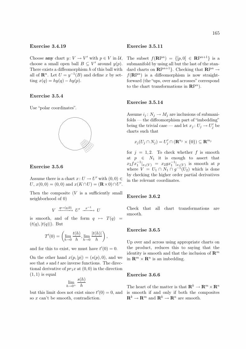
165

Exercise 3.4.19

Choose any chart y : V → V ′ with p ∈ V in U ,choose a small open ball B ⊆ V ′ around y(p).There exists a diffeomorphism h of this ball withall of R

n. Let U = y−1(B) and define x by set-ting x(q) = hy(q)− hy(p).

Exercise 3.5.4

Use “polar coordinates”.

Exercise 3.5.6

Assume there is a chart x : U → U ′ with (0, 0) ∈U , x(0, 0) = (0, 0) and x(K∩U) = (R×0)∩U ′.

Then the composite (V is a sufficiently smallneighborhood of 0)

Vq 7→(q,0)−−−−−→ U ′ x−1

−−−−→ U

is smooth, and of the form q 7→ T (q) =(t(q), |t(q)|). But

T ′(0) =

(limh→0

t(h)

h, limh→0

|t(h)|h

),

and for this to exist, we must have t′(0) = 0.

On the other hand x(p, |p|) = (s(p), 0), and wesee that s and t are inverse functions. The direc-tional derivative of pr1x at (0, 0) in the direction(1, 1) is equal

limh→0+

s(h)

h

but this limit does not exist since t′(0) = 0, andso x can’t be smooth, contradiction.

Exercise 3.5.11

The subset f(RPn) = {[p, 0] ∈ RPn+1} is asubmanifold by using all but the last of the stan-dard charts on RPn+1}. Checking that RPn →f(RPn) is a diffeomorphism is now straight-forward (the “ups, over and acrosses” correspondto the chart transformations in RPn).

Exercise 3.5.14

Assume ij : Nj →Mj are inclusions of submani-folds — the diffeomorphism part of “imbedding”being the trivial case — and let xj : Uj → U ′

j becharts such that

xj(Uj ∩Nj) = U ′j ∩ (Rnj × {0}) ⊆ R

mj

for j = 1, 2. To check whether f is smoothat p ∈ N1 it is enough to assert thatx2fx−1

1 |x1(V ) = x2gx−11 |x1(V ) is smooth at p

where V = U1 ∩ N1 ∩ g−1(U2) which is doneby checking the higher order partial derivativesin the relevant coordinates.

Exercise 3.6.2

Check that all chart transformations aresmooth.

Exercise 3.6.5

Up over and across using appropriate charts onthe product, reduces this to saying that theidentity is smooth and that the inclusion of R

m

in Rm ×R

n is an imbedding.

Exercise 3.6.6

The heart of the matter is that Rk → R

m×Rn

is smooth if and only if both the compositesRk → R

m and Rk → R

n are smooth.


Exercise 3.6.7

Consider the map (t, z) 7→ etz.

Exercise 3.6.8

Reduce to the case where f and g are inclusionsof submanifolds. Then rearrange some coordi-nates to show that case.

Exercise 3.6.9

Use the preceding exercises.

Exercise 3.6.10

Remember that GLn(R) is an open subset ofMn(R) and so this is in flatland 3.5.8). Multi-plication of matrices is smooth since it is madeout of addition and multiplication of real num-bers.

Exercise 3.6.11

Use the fact that multiplication of complexnumbers is smooth, plus 3.5.14).

Exercise 3.6.13

Check chart transformations.

Exercise 3.6.16

Using the “same” charts on both sides, this re-duces to saying that the identity is smooth.

Exercise 3.6.17

A map from a disjoint union is smooth if andonly if it is smooth on both summands since

smoothness is measured locally.

Chapter 4

Exercise 4.2.6

It depends neither on the representation of thetangent vector nor on the representation of thegerm, because if [γ] = [ν] and f = g, then(φfγ)′(0) = (φfν)′(0) = (φgν)′(0) (partially bydefinition).

Exercise 4.3.10

If [γ] = [ν], then (φfγ)′(0) = (φfν)′(0).

Chapter 5

Exercise 5.2.3

See the next exercise. This refers the problemaway, but the same reference helps you out onthis one too!

Exercise 5.2.4

This exercise is solved in the smooth case in ex-ercise 7.2.6. The only difference in the contin-uous case is that you delete every occurence of“smooth” in the solution. In particular, the solu-tion refers to a “smooth bump function φ : U2 →R such that φ is one on (a, c) and zero onU2 \ (a, d)”. This can in our case be chosen tobe the (non smooth) map φ : U2 → R given by

φ(t) =

1 if t ≤ cd−td−c if c ≤ t ≤ d

0 if t ≥ d

167

Exercise 5.4.4

Use the chart domains on RPn from the mani-fold section:

Uk = {[p] ∈ RPn|pk 6= 0}and construct bundle charts π−1(Uk)→ Uk×R

sending ([p], λp) to ([p], λpk). The chart trans-formations then should look something like

([p], λ) 7→ ([p], λplpk

)

If the bundle were trivial, then ηn \ σ0(RPn)would be disconnected. In particular ([e1], e1)and ([e1],−e1) would be in different compo-nents. But γ : [0, π]→ ηn \ σ0(RPn) given by

γ(t) = ([cos(t)e1 + sin(t)e2], cos(t)e1 + sin(t)e2)

is a path connecting them.

Exercise 5.4.5

You may assume that p = [0, . . . , 0, 1]. Then

any point [x0, . . . , xn−1, xn] ∈ X equals[x|x| ,

xn

|x|

]

since x = (x0, . . . , xn−1) must be different from0. Consider the map

X → ηn−1

[x, xn] 7→([

x

|x|

],xnx

|x|2)

with inverse ([x], λx) 7→ [x, λ].

Exercise 5.5.8

View S3 as the unit quaternions, and copy theargument for S1.

Exercise 5.5.9

Lie group is a smooth manifold equipped with asmooth associative multiplication, having a unitand possessing all inverses, so the proof for S1

will work.

Exercise 5.5.13

If we set zj = xj + iyj, x = (x0, . . . , xn) andy = (y0, . . . , yn), then

∑ni=0 z2 = 1 is equiv-

alent to x · y = 0 and |x|2 − |y|2 = 1. Usethis to make an isomorphism to the bundlein example 5.5.10 sending the point (x, y) to(p, v) = ( x

|x| , y) (with inverse sending (p, v) to

(x, y) = (√

1 + |v|2p, v)).

Exercise 5.5.16

Use the trivialization to pass the obvious solu-tion on the product bundle to the tangent bun-dle.

Exercise 5.5.17

Any curve to a product is given uniquely by itsprojections to the factors.

Chapter 6

Exercise 6.2.3

Consider the smooth map

f : G×G→G×G

(g, h) 7→(gh, h)

with inverse (g, h) 7→ (gh−1, h). Use that, fora given g ∈ G, the map G → G sending h togh is a diffeomorphism to conclude that f hasmaximal rank, and is a diffeomorphism. Thenconsider a composite

Gg 7→(1,g)−−−−−→ G×G

f−1

−−−−→ G×G(g,h) 7→g−−−−−→ G


Exercise 6.3.3

Use the rank theorem. To prove that the rankis constant, first prove it for all points in f(M)using the chain rule. See [BJ], Theorem 5.13.That f(M) = {p ∈ M |f(p) = p} is closedin M follows since the complement is open: ifp 6= f(p) choose disjoint open sets U and Varound p and f(p). Then U ∩f−1(V ) is an openset disjoint from f(M) (since U ∩ f−1(V ) ⊆ Uand f(U ∩ f−1(V )) ⊆ V ) containing p.

Exercise 6.4.4

Prove that 1 is a regular value for the functionRn+1 → R sending p to |p|2.

Exercise 6.4.7

Observe that the function in question is

f(eiθ, eiφ) =√

(3− cos θ − cosφ)2 + (sin θ + sinφ)2,

giving the claimed Jacobi matrix. Then solvethe system of equations

3 sin θ − cos φ sin θ + sinφ cos θ =0

3 sinφ− cos θ sinφ + sin θ cos φ =0

Adding the two equations we get that sin θ =sinφ, but then the upper equation claims thatsinφ = 0 or 3− cos φ + cos θ = 0. The latter isclearly impossible.

Exercise 6.4.9

Show that the map

SL2(R)→ (C− {0}) ×R[a bc d

]7→ (a + ic, ab + cd)

is a diffeomorphism, and that S1 ×R is diffeo-morphic to C− {0}.

Exercise 6.4.10

Calculate the Jacobi matrix of the determi-nant function. With some choice of indices youshould get

Dij(det)(A) = (−1)i+jdet(Aij)

where Aij is the matrix you get by deleting theith row and the jth column. If the determinantis to be one, some of the entries in the Jacobimatrix then has got to be nonzero.

Exercise 6.4.12

By corollary 5.5.12 we identify TO(n) with

E =

(g,A) ∈ O(n)×Mn(R)

∣∣∣∣∣∣∣∣

g = γ(0)A = γ′(0)

for some curveγ : (−ε, ε)→ O(n)

That γ(s) ∈ O(n) is equivalent to saying thatI = γ(s)tγ(s). This holds for all s ∈ (−ε, ε), sowe may derive this equation and get

0 =d

ds

∣∣∣∣s=0

(γ(s)tγ(s)

)

= γ′(0)tγ(0) + γ(0)tγ′(0)

= Atg + gtA

Exercise 6.4.14

Consider the chart x : M2(R)→ R4 given by

x

([a bc d

])= (a, b, a− d, b + c).

169

Exercise 6.4.15

Copy one of the proofs for the orthogonal group,replacing the symmetric matrices with Hermi-tian matrices.

Exercise 6.4.16

The space of orthogonal matrices is compactsince it is a closed subset of [−1, 1]n

2. It has at

least two components since the sets of matriceswith determinant 1 is closed, as is the comple-ment: the set with determinant −1.

Each of these are connected since you can getfrom any rotation to the identity through a pathof rotations. One way to see this is to use thefact from linear algebra which says that any el-ement A ∈ SO(n) can be written in the formA = BTB−1 where B and T are orthogonal,and furthermore T is a block diagonal matrixwhere the block matrices are either a single 1on the diagonal, or of the form

T (θk) =

[cos θk − sin θksin θk cos θk

].

So we see that replacing all the θk’s by sθk andletting s vary from 1 to 0 we get a path from Ato the identity matrix.

Exercise 6.4.19

Consider a k-frame as a matrix A with the prop-erty that AtA = I, and proceed as for the or-thogonal group.

Exercise 6.4.21

Either just solve the equation or consider themap

f : P3 → P2

sending y ∈ P3 to f(y) = (y′′)2 − y′ + y(0) +xy′(0) ∈ P2. If you calculate the Jacobian in

obvious coordinates you get that

Df(a0 + a1x + a2x2 + a3x

3) =

1 −1 8a2 00 1 24a3 − 2 24a2

0 0 0 72a3 − 3

The only way this matrix can be singular is ifa3 = 1/24, but the top coefficient in f(a0+a1x+a2x

2 + a3x3) is 36a2

3 − 3a3 which won’t be zeroif a3 = 1/24. By the way, if I did not calculatesomething wrong, the solution is the disjointunion of two manifolds M1 = {2t(1−2t)+2tx+tx2|t ∈ R} and M2 = {−24t2 + tx2 + x3/12|t ∈R}, both diffeomorphic to R.

Exercise 6.4.22

Yeah.

Exercise 6.4.23

Consider the function

f : Rn → R

given by

f(p) = ptAp.

The Jacobi matrix is easily calculated, and usingthat A is symmetric we get that Df(p) = 2ptA.But given that f(p) = b we get that Df(p) ·p =ptAp = b, and so Df(p) 6= 0 if b 6= 0. Hence allvalues but b = 0 are regular. The value b = 0 iscritical since 0 ∈ f−1(0) and Df(0) = 0.

Exercise 6.4.24

For the first case, you may assume that the reg-ular value in question is 0. Since zero is a regularvalue, the derivative in the “fiber direction” hasgot to be nonzero, and so the values of f are pos-itive on one side of the zero section... but thereIS no “one side” of the zero section! This takes


care of all one-dimensional cases, and higher di-mensional examples are excluded since the mapwon’t be regular if the dimension increases.

Exercise 6.4.25

You don’t actually need theorem 6.4.3 to provethis since you can isolate T in this equation, andshow directly that you get a submanifold dif-feomorphic to R

2, but still, as an exercise youshould do it by using theorem 6.4.3.

Exercise 6.4.26

Code a flexible n-gon by means of a vectorx0 ∈ R

2 giving the coordinates of the first point,and vectors xi ∈ S1 going from point i to pointi+1 for i = 1, . . . , n−1 (the vector from point nto point 1 is not needed, since it will be given bythe requirement that the curve is closed). Theset R

2 × (S1)n−1 will give a flexible n-gon, ex-cept, that the last line may not be of length 1.To ensure this, look at the map

f : Rk × (Sk−1)n−1 → R

(x0, (x1, . . . , xn−1)) 7→∣∣∣∣∣n−1∑

i=1

xi

∣∣∣∣∣

2

and show that 1 is a regular value. If you letxj = eiφj and x = (x0, (x1, . . . , xn−1)), you getthat

Djf(x) = Dj

((

n−1∑

k=1

eiφk)(

n−1∑

k=1

e−iφk)

)

= ieiφj (

n−1∑

k=1

e−iφk) + (

n−1∑

k=1

eiφk)(−ie−iφj )

= −2Im

(eiφj (

n−1∑

k=1

e−iφk)

)

That the rank is not 1 is equivalent to Djf(x) =0 for all j. Analyzing this, we get thatx1, . . . , xn−1 must then all be paralell. But this

is impossible if n is odd and∣∣∣∑n−1

i=1 xi∣∣∣2

= 1.

(Note that this argument fails for n even. Ifn = 4 LF4,2 is not a manifold: given x1 andx2 there are two choices for x3 and x4: (eitherx3 = −x2 and x4 = −x1 or x3 = −x1 andx4 = −x2), but when x1 = x2 we get a crossingof these two choices).

Exercise 6.4.27

The non-self-intersecting flexible n-gons form anopen subset.

Exercise 6.5.2

It is clearly injective, and an immersion since ithas rank 1 everywhere. It is not an imbeddingsince R

∐R is disconnected, whereas the image

is connected.

Exercise 6.5.3

It is clearly injective, and immersion since it hasrank 1 everywhere. It is not an imbedding sincean open set containing a point z with |z| = 1 inthe image must contain elements in the imageof the first summand.

Exercise 6.5.6

If a/b is irrational then the image of fa,b is dense:that is any open set on S1 × S1 intersects theimage of fa,b.

Exercise 6.5.7

Show that it is an injective immersion homeo-morphic to its image. The last property followssince both the maps in

M −−−−→ i(M) −−−−→ ji(M)

171

are continuous and bijective and the compositeis a homeomorphism.

Chapter 7

Exercise 7.2.1

The only problem is in the origin. If you calcu-late

limt→0+

1

t(λ(t)− λ(0)) = lim

t→0+

e−1/t2

t

= lims→∞

se−s2

= 0

you see that λ is once differentiable, and it con-tinues this way proving that λ is smooth.

Exercise 7.2.3

Let φ : Uφ → R be a representative for φ, and let(x,U) be any chart around p such that x(p) = 0.Choose an ε > 0 such that x(U ∩ Uφ) containsthe open ball of radius ε. Then the germ repre-sented by φ is equal to the germ represented bythe map defined on all of M given by

q 7→{

γ(ε/3,ε/3)(x(q))φ(q) for q ∈ U ∩ Uφ

0 otherwise.

Exercise 7.2.4

You can extend any chart to a function definedon the entire manifold.

Exercise 7.2.5

Smoothen up the proof you gave for the samequestion in the vector bundle chapter, or useparts of the solution of exercise 7.2.6.

Exercise 7.2.6

Let π : E → S1 be a one-dimensional smoothvector bundle (one-dimensional smooth vec-tor bundles are frequently called line bundles).Since S1 is compact we may choose a finite bun-dle atlas, and we may remove superfluous bun-dle charts, so that no domain is included in an-other. We may also assume that all chart do-mains are connected. If there is just one bundlechart, we are finished, otherwise we proceed asfollows. If we start at some point, we may orderthe charts, so that they intersect in a nonemptyinterval (or a disjoint union of two intervals ifthere are exactly two charts). Consider twoconsecutive charts (h1, U1) and (h2, U2) and let(a, b) be (one of the components of) their inter-section. The transition function

h12 : (a, b)→ R \ {0} ∼= GL1(R)

must take either just negative or just positivevalues. Multiplying h2 by the sign of h12 we geta situation where we may assume that h12 al-ways is positive. Let a < c < d < b, and choosea smooth bump function φ : U2 → R such thatφ is one on (a, c) and zero on U2 \ (a, d). Definea new chart (h′

2, U2) by letting

h′2(t) =

(φ(t)

h12(t)+ 1− φ(t)

)h2(t)

(since h12(t) > 0, the factor by which we multi-ply h2(t) is never zero). On (a, c) the transitionfunction is now constantly equal to one, so ifthere were more than two charts we could mergeour two charts into a chart with chart domainU1 ∪ U2.

So we may assume that there are just two charts.Then we may proceed as above on one of thecomponents of the intersection between the twocharts, and get the transition function to be theidentity. But then we would not be left with theoption of multiplying with the sign of the transi-tion function on the other component. However,by the same method, we could only make it plus


or minus one, which exactly correspond to thetrivial bundle and the canonical line bundle.

Just the same argument shows that there are ex-actly two isomorphism types of n-dimensionalsmooth vector bundles over S1 (using thatGLn(R) has exactly two components). Thesame argument also gives the correspondingtopological fact.

Chapter 8

Exercise 8.1.4

As an example, consider the open subset U 0,0 ={eiθ ∈ S1| cos θ > 0}. The bundle charth : U0,0×C→ U0,0×C given by sending (eiθ, z)to (eiθ, e−iθ/2z). Then h((U 0,0 × C) ∩ η1) =U0,0 ×R. Continue this way all around the cir-cle. The idea is the same for higher dimensions:locally you can pick the first coordinate to beon the line [p].

Exercise 8.1.11

Let Xk = {p ∈ X|rkpf = k}. We want to showthat Xk is both open and closed, and hence ei-ther empty or all of X since X is connected.

Let P = {A ∈ Mm(A)|A = A2}, then Pk ={A ∈ P |rk(A) = k} ⊆ P is open. To see this,write Pk as the intersection of P with the twoopen sets

{A ∈Mn(R)|rkA ≥ k}and

A ∈Mn(R)

∣∣∣∣∣∣∣∣∣∣

A has less thanor equal to k

linearly independenteigenvectors with

eigenvalue 1

.

But, given a bundle chart (h,U), then the map

Up7→hpfph

−1p−−−−−−−→ P

is continuous, and hence U ∩ Xk is open in U .Varying (h,U) we get that Xk is open, andhence also closed since Xk = X \⋃i6=k Xi.

Exercise 8.1.12

Use exercise 8.1.11 to show that the bundle map12(idE − f) has constant rank (here we use thatthe set of bundle morphisms is in an obviousway a vector space).

Exercise 8.2.4

A×X E = π−1(A).

Exercise 8.2.5

This is not as complex as it seems. For instance,the map E → f∗E = X ′ ×X E must send e to(π(e), g(e)) for the diagrams to commute.

Exercise 8.2.6

If h : E → X ×Rn is a trivialization, then the

map f∗E = Y ×X E → Y ×X (X×Rn) induced

by h is a trivialization, since Y ×X (X ×Rn)→

Y ×Rn sending (y, (x, v)) to (y, v) is a homeo-

morphism.

Exercise 8.2.7

X ×Y (Y ×Z E) ∼= X ×Z E.

Exercise 8.3.2

The transition functions will be of the typeU 7→ GLn1+n2(R), which sends p ∈ U to theblock matrix

[(h1)p(g1)

−1p 0

0 (h2)p(g2)−1p

]

173

which is smooth if each of the blocks are smooth.Similarly for the morphisms.

Exercise 8.3.4

Use the map ε → Sn × R sending (p, λp) to(p, λ).

Exercise 8.3.6

Consider TSn ⊕ ε, where ε is gotten from exer-cise 8.3.4. Construct a trivialization TSn⊕ ε→Sn ×R

n+1.

Exercise 8.3.7

ε1 ⊕ ε2h1⊕h2−−−−→

∼=X × (Rn1 ⊕R

n2)

(E1 ⊕E2)⊕ (ε1 ⊕ ε2) ∼= (E1 ⊕ ε1)⊕ (E2 ⊕ ε2)

Exercise 8.3.8

Given f1 and f2, let f : E1 ⊕ E2 → E3 begiven by sending (v, w) ∈ π−1

1 (p) ⊕ π−12 (p) to

f1(v) + f2(w) ∈ π−13 (p). Given f let f1(v) =

f(v, 0) and f2(w) = f(0, w).

Exercise 8.4.4

Send the bundle morphism f to the sectionwhich to any p ∈ X assigns the linear mapfp : Ep → E′

p.

Exercise 8.4.6

Let F ⊆ E be a k-dimensional subbundle of then-dimensional vector bundle π : E → X. Defineas a set

E/F =∐

p∈X

Ep/Fp

with the obvious projection π : E/F → X. Thebundle atlas is given as follows. For p ∈ Xchoose bundle chart h : π−1(U)→ U ×R

n suchthat h(π−1(U) ∩ F ) = U ×R

k × {0}. On eachfiber this gives a linear map on the quotienthp : Ep/Fp → R

n/Rk × {0} via the formula

hp(v) = hp(v) as in 2. This gives a function

h : (π)−1(U) =∐

p∈U

Ep/Fp

→∐

p∈U

Rn/Rk × {0}

∼= U ×Rn/Rk × {0}

∼=U ×Rn−k.

You then have to check that the transition func-tions p 7→ gph

−1p = gph

−1p are continuous (or

smooth).

As for the map of quotient bundles, this followssimilarly: define it on each fiber and check con-tinuity of “up, over and down”.

Exercise 8.4.7

Altk(E) =∐p∈X AltkEp and so on.

Exercise 8.4.8

The transition functions on L → M are mapsinto nonzero real numbers, and on the tensorproduct this number is squared, and so all tran-sition functions on L ⊗ L → M map into pos-itive real numbers. Use partition of unity toglue these together and scale them to be theconstantly 1.

Exercise 8.6.5

Note that the map in question induces a linearmap on every fiber which is an isomorphism,and hence by lemma 5.3.12 the map is an iso-morphism of bundles.


Exercise 8.6.8

Use lemma 8.6.2 and exercise 8.6.5 to showthat the bundle in question is isomorphic to(TR

n)|M →M .

Exercise 8.6.9

You have done this exercise before!

Exercise 8.6.10

Prove that the diagonal M → M × M is animbedding by proving that it is an immersioninducing a homeomorphism onto its image. Thetangent space of the diagonal at (p, p) is exactlythe diagonal of T(p,p)(M ×M) ∼= TpM × TpM .For any vector space V , the quotient spaceV × V/diagonal is canonically isomorphic to Vvia the map given by sending (v1, v2) ∈ V × Vto v1 − v2 ∈ V .

Exercise 8.7.6

Show that the map

f × g : M × L→ N ×N

is transverse to the diagonal (which is discussedin exercise 8.6.10), and that the inverse imageof the diagonal is exactly M ×N L.

Exercise 8.8.1

The conditions you need are exactly the onesfulfilled by the elementary definition of the de-terminant: check your freshman introduction.

Exercise 8.9.1

Check out e.g. [MS] page 57.

Exercise 8.9.2


Exercise 8.9.4


Chapter 9

Exercise 9.1.4

Check the two defining properties of a flow. Asan aside: this flow could be thought of as theflow R×C→ C sending (t, z) to e−z−t/2, whichobviously satisfies the two conditions.

Exercise 9.1.19

Consider one of the “bad” injective immersionsthat fail to be imbeddings, and force a disconti-nuity on the velocity field.

Exercise 9.2.3

Consider a bump function phi on the spherewhich is 1 near the North pole and 0 near theSouth pole. Consider the vector field Z =

φ→Φ + (1 − φ)

→Ψ. Near the North pole Z =

→Φ

and near the South pole Z =→Ψ, and so the flow

associated with Z has the desired properties.

Exercise 9.2.4

The vector field associated with the flow

Φ: R× (S1 × S1)→ (S1 × S1)

given by Φ(t, (z1, z2)) = (eiatz1, eibtz2) exhibits

the desired phenomena when varying the realnumbers a and b.

175

Exercise 9.2.5

All we have to show is that X is the velocityfield of Φ. Under the diffeomorphism

TO(n)→E

[γ]→(γ(0), γ ′(0))

this corresponds to the observation that

∂

∂s

∣∣∣∣s=0

Φ(s, g) = gA.

Exercise 9.5.8

Concerning the map ` : S1 → CP1: note that itmaps into a chart domain on which lemma tellsus that the projection is trivial.

Exercise 9.4.5

Do a variation of example 9.3.3.

Exercise 9.5.9

Write R as a union of intervals Jj so that foreach j, γ(Uj) is contained within one of the opensubsets of M so that the fibration trivializes. Oneach of these intervals the curve lifts, and youmay glue the liftings using bump functions.

Exercise 9.6.3

There is no hint beyond: use the definitions!

Exercise 9.6.4

Use the preceding exercise: notice that TπMξ =πTMξ is necessary for things to make sense sinceγ had two repeated coordinates.

Exercise 9.6.8

The conditions the sections have to satisfy areconvex, just as in the proof of existence of Rie-mannian structures.

Exercise 9.6.9

The thing to check is that T is an open neigh-borhood of the zero section.

Chapter 10

Exercise 10.1.5

Consider the union of the closed intervals[1/n, 1] for n ≥ 1)

Exercise 10.1.7

Consider the set of all open subsets of X con-tained in U . Its union is open.

Exercise 10.1.9

By the union axiom for open sets, int A is openand contains all open subsets of A.

Exercise 10.1.10

The intersection of two open balls is the unionof all open balls contained in the intersection.

Exercise 10.1.11

All open intervals are open balls!


Exercise 10.2.2

Hint one way: the “existence of the δ” assuresyou that every point in the inverse image has asmall interval around it inside the inverse imageof the ε ball.

a

U

f (U)−1

Exercise 10.2.3

f−1(g−1(U)) = (gf)−1(U).

Exercise 10.2.6

Use first year calculus.

Exercise 10.3.3

Can you prove that the set containing only theintervals (a, b) when a and b varies over the ra-tional numbers is a basis for the usual topologyon the real numbers?

Exercise 10.3.4

Show that given a point and an openball con-taining the point there is a “rational” ball inbetween.

Exercise 10.3.5

Use note 10.3.2.

Exercise 10.3.6

f−1(⋃α Vα) =

⋃α f−1(Vα).

Exercise 10.5.2

Use that (⋃α Uα) ∩ A =

⋃α (Uα ∩A) and

(⋂α Uα) ∩A =

⋂α (Uα ∩A).

Exercise 10.5.3

Use 10.2.3 one way, and that if f−1(U ∩ A) =f−1(U) the other.

Exercise 10.5.4

The intersections of A with the basis elementsof the topology on X will form a basis for thesubspace topology on A.

Exercise 10.5.5

Separate points in A by means of disjoint neigh-borhoods in X, and intersect with A.

Exercise 10.6.2

Inverse image commutes with union and inter-section.

Exercise 10.6.3

Use 10.2.3 one way, and the characterization ofopen sets in X/ ∼ for the other.

177

Exercise 10.6.4

Show that open sets in one topology are openin the other.

Exercise 10.7.2

Cover f(X) ⊆ Y by open sets i.e. by sets of theform V ∩ f(X) where V is open in Y . Sincef−1(V ∩ f(X)) = f−1(V ) is open in X, thisgives a covering of X. Choose a finite subcover,and select the associated V ’s to cover f(X).

Exercise 10.7.5

The real projective space is compact by 10.7.2.The rest of the claims follows by 10.7.11, butyou can give a direct proof by following the out-line below.

For p ∈ Sn let [p] be the equivalence class of pconsidered as an element of RPn. Let [p] and [q]be two different points. Choose an ε such thatε is less than both |p− q|/2 and |p+ q|/2. Thenthe ε balls around p and −p do not intersect theε balls around q and −q, and their image definedisjoint open sets separating [p] and [q].

Notice that the projection p : Sn → RPn sendsopen sets to open sets, and that if V ⊆ RPn,then V = pp−1(V ). This implies that the count-able basis on Sn inherited as a subspace of Rn+1

maps to a countable basis for the topology onRPn.

Exercise 10.7.9

You must show that if K ⊆ C is closed, then(f−1

)−1(K) = f(K) is closed.

Exercise 10.7.10

Use Heine-Borel 10.7.3 and exercise 10.7.2.

Exercise 10.8.2

One way follows by 10.2.3. For the other, ob-serve that by exercise 10.3.6 it is enough to showthat if U ⊆ X and V ⊆ Y are open sets, thenthe inverse image of U × V is open in Z.

Exercise 10.8.3

Show that a square around any point containsa circle around the point and vice versa.

Exercise 10.8.4

If B is a basis for the topology on X and C is abasis for the topology on Y , then

{U × V |U ∈ B, V ∈ C}

is a basis for X × Y .

Exercise 10.8.5

If (p1, q1) 6= (p2, q2) ∈ X × Y , then eitherp1 6= p2 or q1 6= q2. Assume the former, andlet U1 and U2 be two open sets in X separatingp1 and p2. Then U1 × Y and U2 × Y are. . .

Exercise 10.9.2

The inverse image of a set that is both open andclosed is both open and closed.

Exercise 10.9.4

Both X and Y are open sets.


Exercise 10.9.5

One way follows by 10.2.3. The other followssince an open subset of X

∐Y is the (disjoint)

union of an open subset of X with an open sub-set of Y .

Exercise 10.11.5

If p ∈ f(f−1(B)) then p = f(q) for a q ∈f−1(B). But that q ∈ f−1(B) means simplythat f(q) ∈ B!

Exercise 10.11.6

These are just rewritings.

Exercise 10.11.7

We have that p ∈ f−1(B1∩B2) iff f(p) ∈ B1∩B2

iff f(p) is in both B1 and B2 iff p is in both

f−1(B1) and f−1(B2) iff p ∈ f−1(B1)∩f−1(B2).The others are equally fun.

Bibliography

[BJ] Bröcker, Th. and Jänich, Introduction to differential topology. Translated fromthe German by C. B. Thomas and M. J. Thomas. Cambridge University Press,Cambridge-New York, 1982. vii+160 pp. ISBN: 0-521-24135-9; 0-521-28470-8 58-01(57Rxx)

[H] Hirsch, Morris W. Differential topology. Corrected reprint of the 1976 original. Grad-uate Texts in Mathematics, 33. Springer-Verlag, New York, 1994. x+222 pp. ISBN:0-387-90148-5 57-01 (58-01)

[M] Milnor, John W. Topology from the differential viewpoint. Based on notes by DavidW. Weaver. Revised reprint of the 1965 original. Princeton Landmarks in Mathemat-ics. Princeton University Press, Princeton, NJ, 1997. xii+64 pp. ISBN: 0-691-04833-957Rxx

[MS] Milnor, John W. and Stasheff, James D. Characteristic classes. . Annals of Mathe-matics Studies, No. 76. Princeton University Press, Princeton, N. J.; University ofTokyo Press, Tokyo, 1974. vii+331 pp. 57-01 (55-02 55F40 57D20)

[S] Spivak, Micheal, A comprehensive introduction th differential geometry.Vol. I. Secondedition. Publish or Perish, Inc., Wilmington, Del., 1979. xiv+668 pp. ISBN: 0-914098-83-7 53-01

[SC] Spivak, Micheal, Calculus on manifolds. A modern approach to classical theorems ofadvanced calculus. W. A. Benjamin, Inc., New York-Amsterdam 1965 xii+144 pp.26.20 (57.00)

179

Index

C∞(M), 33C∞(M,N), 33D,_pM52En: the open n-disk, 22Gkn, 86

L : R×R→ R, 125MnR, 37Mm×nR, 37M r

m×nR, 37O(n), 83SLn(R), 83SO(n), 86Sn: the n-sphere, 22TpM , 47TpM ∼= D,_pM55Tpf , 49U(n), 86V kn , 86

[γ] = [γ], 47≈, 47f , germ represented by f , 44C∞=smooth, 30D, 28GLn(R), 37ξ(M, p), 46f ∗ : ξ(f(p))→ ξ(p), 46k-frame, 86pri, 46rkpf , 75supp(f), 93

alternating forms, 111atlas, 21

bundle, 60good, 97maximal, 29

smooth bundle, 63

bad taste, 60base space, 60basis for the topology, 148bijective, 155Borromean rings, 41bump function, 95bundle

atlas, 60smooth, 63

chart, 60chart transformation, 62morphism, 61

smooth, 65

canonical n-plane bundle, 121canonical line bundle, 60chain rule, 49chain rule, the, 160chart, 21

domain, 21transformation, 24

closed set, 146closure, 146compact space, 150complement, 146, 154complex projective space, CPn, 28composition of germs, 45connected space, 152connected sum, 16constant rank, 103continuous

map, 147coordinate functions

standard, 46

180

INDEX 181

countable basis, 148critical, 76

De Morgan’s formulae, 154derivation, 52determinant function, 119diffeomorphic, 32diffeomorphism, 25, 32differentiable manifold, 30differentiable map, 31differential=smooth, 30disjoint union, 40, 152dual space, 110

Ehresmann’s fibration theorem, 140Ehresmann’s fibration theorem, 137embedding=imbedding, 38equivalence

class, 154relation, 154

existence of maxima, 151exponential map, 143exterior power, 111

family, 154fiber, 60fiber product, 105, 119fixed point free involution, 34flow

global, 124local, 133maximal local, 134

flow line, 126, 134function germ, 46fusion reactor, 73

generalized Gauss map, 122generate (a topology), 148genus, 16geodesic, 142germ, 44good atlas, 97Grassmann manifold, 86, 121

handle, 16

Hausdorff space, 149Heine–Borel’s theorem, 151hom-space, 110homeomorphic, 147homeomorphism, 147Hopf fibration, 140

image, 155of bundle morphism, 105of map of vector spaces, 104

imbedding, 38immersion, 81induced bundle, 105injective, 155Integrability theorem, 130, 134interior, 146intermediate value theorem, 152inverse function theorem, 77, 160inverse image, 155isomorphism of smooth vector bundles, 65

Jacobi matrix, 54Jacobian matrix, 159

kernelof bundle morphism, 105of map of vector spaces, 104

labelled flexible n-gons, 87Leibnitz rule, 52Lie Group

S1 is one, 40Lie group

O(n), 85SLn(R), 85U(n), 86GLn(R) is one, 40

line bundle, 173line bundle, 63, 96local diffeomorphism, 34local flow, 133local trivialization, 60locally trivial fibration, 136locally finite, 93

182 INDEX

locally homeomorphic, 21locally trivial, 60

magnetic dipole, 73manifold

smooth, 30topological, 21

maximal local flow, 134maximal (smooth) bundle atlas, 64maximal atlas, 29metric topology, 146morphism

of bundles, 61

neighborhood, 146nonvanishing section, 62normal bundle

of a submanifold, 116of an imbedding, 116w.r.t. a Riemannian metric, 115

one-to-one, 155onto, 155open ball, 146open set, 146open submanifold, 37orbit, 126, 134orientable, 15orientable bundle, 120orientable manifold, 120orientation

of a vector bundle, 120on a vector space, 120

orientation preserving isomorphism, 120orientation reversing isomorphism, 120orientation class, 120oriented vector space, 120orthogonal matrices, 83

parallelizable, 70partial derivative, 159partition of unity, 94periodic immersion, 129pre-bundle atlas, 67

pre-vector bundle, 67precomposition, 46preimage, see inverse imageproduct

smooth, 39space, 152topology, 152

product bundle, 61projections (from the product), 152proper, 137

quadric, 87quotient

space, 150topology, 150

quotient bundle, 113quotient space, 110

rank, 75constant, 75

rank theorem, 79real projective space, RPn, 23, 28refinement, 97reflexivity, 154regular

point, 76value, 76

represent, 44restriction, 149restriction of bundle, 102Riemannian manifold, 114Riemannian metric, 114

Sard’s theorem, 76second order differential equation, 141section, 61singular, 76skew matrix, 85smooth

bundle morphism, 65bundle atlas, 63manifold, 30map, 31map, at a point, 31

INDEX 183

pre-vector bundle, 67structure, 30vector bundle, 64

solution curvefor first order differential equation, 130for second order differential equation,

142special linear group, 83special orthogonal group, 86sphere, (standard smooth), 30stably trivial, 109stereographic projection, 26Stiefeld manifold, 86subbundle, 101submanifold, 35

open, 37submersion, 81subordinate, 94subspace, 149sum, of smooth manifolds, 40support, 93surjective, 155symmetric power, 111symmetric bilinear form, 112symmetry, 154

tangent spacegeometric definition, 47

tensor product, 110topological space, 146topology, 145

on a space, 146torus, 39total space, 60transition function, 62transitivity, 154transverse, 117trivial

smooth vector bundle, 64trivial bundle, 61

unitary group, 86

van der Waal’s equation, 87

vector bundlen-dimensional (real topological), 59smooth, 64

vector field, 72velocity vector, 127velocity field, 125, 134

Whitney sum, 108

zero section, 61

di˙erential topology - mathematicswsw/s05/dun.pdf · the appendix covering the bare essentials of...

Documents