Diet composition of wolves (Canis lupus) on the

Scandinavian peninsula determined by scat analysis

r

Sabrina Müller

Sweden, July 2006

© S. Mülle

If you talk to the animals they will talk with you and you will know each other.

If you do not talk to them you will not know them,

and what you do not know you will fear.

What one fears one destroys.

Chief Dan George (1899-1981)

Preface This paper is the English summarization of the thesis ‘Saisonale Variation im Nahrungsspektrum

des Wolfes in Skandinavien. Oder: Was ist wirklich drin im Wolfskot?’ (30 ECTS) submitted to

the School of Forest Science and Resource Management, Technical University of Munich (Germany)

in partial fulfilment of the requirements for the diploma degree in Forest Science.

Due to the collaborative nature of this work, in particular the scat collection and scat analysis, I have

used the term ‘we’ instead of ‘I’ in this paper. I did all of the data analysis and writing and take full

responsibility for any errors contained in this paper.

Abstract Seasonal diet composition of wolves (Canis lupus) was studied on the Scandinavian Peninsula by

analysing 2063 wolf scats. The scats were collected during summer and winter of the years 1992 to

2005. A reduced data set (n = 1594) was used to describe the seasonal feeding pattern of 10

Scandinavian wolf territories in detail.

Although the diverse diet confirmed the wolves’ nature as opportunistic predators, moose was the

most common item in percent frequency of occurrence in summer (53.7%) and winter (68.5%),

representing 88.9% and 95.7% of the mammalian biomass consumed in summer and winter,

respectively. Other prey species like roe deer, beaver, badger, hare, small rodents and birds were

regularly used during the year, with emphasis on the summer months. Within the studied period

domestic animals only contributed marginally to the diet of wolves. Nevertheless, domestic animals

were more frequently identified in summer than in winter with 1.3% and 0.1%, respectively.

Moose was the preferred prey in summer (Manly’s Alpha = 0.68) and winter (Manly’s Alpha = 0.54).

Food niche breadth was broader in summer (BA = 0.11) than in winter (BA = 0.04). This may be

explained by the higher availability of smaller prey species like beaver, hare, small rodents and birds

during the summer period.

The diet pattern described for the sub sample of 10 Scandinavian territories did not differ from the

pattern shown by the remaining sample. The interterritorial comparison showed a high similarity

among the seasons as well. Only two territories located in areas with comparably high roe deer

densities differed from the others with respect to moose:roe deer ratio determined by the analysis of

summer and winter scats.

In comparison to previous studies on the foraging ecology of wolves in Scandinavia, moose appeared

to be even more frequently consumed, also in areas with high roe deer densities.

2

1 Introduction

The conflict between humans and wolves has always been grounded on the wolf’s role as predator on

wild game and domestic animals. Therefore a detailed knowledge on the seasonal diet composition is

fundamental for a better understanding of wolves as predators and for the management of prey as well

as predator populations. Since the pioneering work of Murie in the 1940s on the foraging behaviour of

wolves in Denali National Park (MECH & BOITANI 2003), innumerable studies have been carried out

world-wide to investigate predation ecology.

Although the diet of wolves appears to be diverse and opportunistic (SALVADOR & ABAD 1987,

CUESTA et al. 1991), it is evident that wild ungulates constitute the main prey type (i.a. BALLARD et al.

1987, KOHIRA & REXSTAD 1997, JĘDRZEJEWSKI et al. 2000). Depending on the local availability,

wolves mainly prey on middle-sized wild ungulates such as white-tailed deer (Odocoileus

virginianus), red deer (Cervus elaphus), reindeer (Rangifer tarandus), roe deer (Capreolus capreolus)

and wild boar (Sus scrofa) (i.a. SCOTT & SHACKLETON 1980, BALLARD et al. 1987, POTVIN et al.

1988, SIDOROVICH et al. 2003, NOWAK et al. 2005). In boreal conifer forest landscapes moose (Alces

alces) is an important prey species for wolves as well (i.a. THEBERGE & COTTRELL 1977, PETERSON

et al. 1984, KOJOLA et al. 2004).

In areas where wolves live in close neighbourhood to humans, anthropogenic food sources such as

garbage or domestic animals are also used by the large carnivores (FRITTS & MECH 1981, SALVADOR

& ABAD 1987, SIDOROVICH et al. 2003, THEUERKAUF 2003, CHAVEZ & GESE 2005, GAZZOLA et al.

2005, NOWAK et al. 2005). Predation on domestic animals causes the biggest problems with humans.

This is also evident on the Scandinavian peninsula where 400 to 600 sheep are killed by wolves

annually. (SWEDISH WILDLIFE DAMAGE CENTRE 2004). However, GAZZOLA et al. (2005) and

ANSORGE et al. (2006) argue that wolves prefer wild ungulates to domestic ungulates if the wild prey

is available in adequate numbers.

On the Scandinavian peninsula numerous studies have been carried out on predation ecology of

wolves (PALM 2001, WIKENROS 2001, JOHANSSON 2004, PEDERSEN et al. 2005, SAND et al. 2005,

SAND et al. 2006, SAND et al. in press), whereas most of the studies have been performed during the

winter months. With the help of carcass search it was possible to describe that moose is the

predominant prey for wolves in Scandinavia, followed by roe deer.

The only studies on wolf diet in Scandinavia based on scat analyses have been performed by

OLSSON et al. (1997) and ØSTRENG (2000). Both studies describe a higher importance of roe deer than

it was observed in previous studies. The data published by ØSTRENG (2000) was also collected within

a SKANDULV research project. Therefore the dataset was included into our study to provide more

detailed information about the diet of wolves in Norwegian territories.

3

The aim of this study was to describe the diet composition of wolves in Scandinavia in summer and

winter on an area-wide scale. We chose scat analysis as the method to identify prey items consumed.

In contrast to carcass search we were able to cover a larger study area as well as a larger study period

and it was possible to identify prey species that are usually consumed completely and therefore not

detectable with carcass search. Since we were also interested in the seasonal utilization of plant

material and small rodents, scat analysis was a suitable research method. To describe the seasonal

foraging pattern of wolves on the Scandinavian peninsula we were interested into the following

questions:

• Is there a difference in diet composition between summer and winter?

• What is the preferred prey for wolves?

• How important is alternative and smaller prey such as beaver, badger, hare, birds and small

rodents in both seasons?

• Is there a difference in Food Niche Breadth in summer and winter and is the Food Niche

Breadth influenced by prey densities?

We also compared the conventional methods to calculate biomass consumed to show the differences

between the methods and to look for criterions how to choose an adequate method for a given study.

2 Study area

The study area is located in the south-central part of the Scandinavian peninsula (Sweden and

Norway) between lat 59°N and 61°N, long 11°W and 16°W (Figure 1). The area is mostly covered

with boreal forest dominated by Scots pine (Pinus sylvestris) and Norway spruce (Picea abies),

sometimes intermixed with deciduous trees like birch (Betula verrucosa, B. pubescens), aspen

(Populus tremula), and alder (Alnus incana, A. glutinosa). Agricultural land prevails in the southern

part of the study area. Forestry practices on the Scandinavian peninsula result in small scale mosaics

of forests of different densities and age classes as well as clearings with pioneer vegetation including

birch (Betula spec.) and dwarf shrubs such as blueberry (Vaccinium spec.) and heather (Calluna

vulgaris).

The area is hilly with altitude ranging from 50m to 1000m a.s.l. The climate is characterized as

continental with mean temperature of 15°C in July and –7°C in January. Normally the ground is

covered with snow from December till March, and mean snow depth is between 20cm and 50cm.

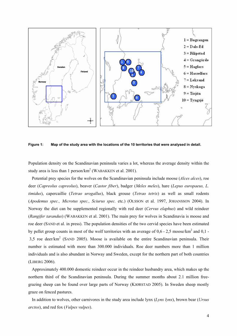
Figure 1: Map of the study area with the locations of the 10 territories that were analysed in detail.

Population density on the Scandinavian peninsula varies a lot, whereas the average density within the

study area is less than 1 person/km2 (WABAKKEN et al. 2001).

Potential prey species for the wolves on the Scandinavian peninsula include moose (Alces alces), roe

deer (Capreolus capreolus), beaver (Castor fiber), badger (Meles meles), hare (Lepus europaeus, L.

timidus), capercaillie (Tetrao urogallus), black grouse (Tetrao tetrix) as well as small rodents

(Apodemus spec., Microtus spec., Sciurus spec. etc.) (OLSSON et al. 1997, JOHANSSON 2004). In

Norway the diet can be supplemented regionally with red deer (Cervus elaphus) and wild reindeer

(Rangifer tarandus) (WABAKKEN et al. 2001). The main prey for wolves in Scandinavia is moose and

roe deer (SAND et al. in press). The population densities of the two cervid species have been estimated

by pellet group counts in most of the wolf territories with an average of 0,6 - 2,5 moose/km2 and 0,1 -

3,5 roe deer/km2 (SAND 2005). Moose is available on the entire Scandinavian peninsula. Their

number is estimated with more than 300.000 individuals. Roe deer numbers more than 1 million

individuals and is also abundant in Norway and Sweden, except for the northern part of both countries

(LIBERG 2006).

Approximately 400.000 domestic reindeer occur in the reindeer husbandry area, which makes up the

northern third of the Scandinavian peninsula. During the summer months about 2.1 million free-

grazing sheep can be found over large parts of Norway (KJØRSTAD 2005). In Sweden sheep mostly

graze on fenced pastures.

In addition to wolves, other carnivores in the study area include lynx (Lynx lynx), brown bear (Ursus

arctos), and red fox (Vulpes vulpes).

4

5

3 Material and Methods

Scats were randomly collected on travel routes, carcass sites, den sites, and rendezvous sites from

1991 to 2006. The scats were stored in labelled plastic bags indicating location and date, and were

frozen until further analyses at the Grimsö Research Station. Prior to the analyses the scats were dried

for 48h at 90°C (±5°C). After the drying process, dry weight of the scats was taken (0,01g precision).

Altogether 2799 scats were collected, whereof 2063 scats were chosen for the diet analysis. For

seasonal comparisons among territories at least 15-20 scats per territory and season were required

(SAND unpublished data, ELMHAGEN et al. 2002). As soon as these criterions were fulfilled, the scats

were chosen randomly. The total sample was subdivided into 2 sub samples: 1 summer (May 01–

September 30; n = 794) and 1 winter sample (October 01 – April 30; n = 1238). 31 blank dated scats

needed to be excluded from the seasonal comparison, but were integrated into the total representation.

The procedure to analyse the scat contents followed SPAULDING et al. (1997). Each scat was broken

apart by hand and the single prey items were sorted. If there was more than one prey item found in the

scat, we assumed that the macro and micro components originated from the found items in the same

proportion (CIUCCI et al. 1996). We identified the macro components in the scats (e.g. bird remains,

hairs, hooves, teeth) with the help of reference manuals (MOORE et al. 1974, DEBROT et al. 1982,

TEERINK 1991) and a reference collection developed at the Grimsö Research Station. The hairs were

first examined visually concerning colour pattern, length, thickness, and thereafter identified

microscopically by medullary pattern and cuticular scale (TEERINK 1991). With the help of a reference

grid we visually estimated the relative volumetric proportion for each prey item identified in a scat

(REYNOLDS & AEBISCHER 1991).

Prior to the analyses the observers were trained in identifying scat contents by practicing with

reference material and reference scats. As recommended by CIUCCI et al. (1996), MECH & BOITANI

(2003) and MATTIOLI et al. (2004) a blind test was performed with 30 scat samples to assess the

accuracy of identification by the laboratory personal. The errors were below the threshold of 5%

(MATTIOLI et al. 2004).

The prey items identified in the scats were pooled into the following categories:

moose beaver domestic animals

roe deer hare insects

badger small rodents berries

fox forest birds plant material

wolf birds others

The category ‘others’ represents non food items like stones, leather, and plastic. If it was not possible

to identify a prey item correctly, we rather grouped those items into the following categories than

6

identifying them wrong: undetermined cervids (represents moose and roe deer), undetermined

carnivores, undetermined mammals (REYNOLDS & AEBISCHER 1991).

The distinction into juvenile and adult cervids was carried out due to the characteristic hair pattern

of young animals. We were not able to distinguish consistently between juvenile and adult animals

because the typical juvenile hair pattern is only visible from birth to the first autumn molt in August /

September. Because of that it is not possible to distinguish between juveniles and adults during the

winter season by looking at the hairs (JAMES 1983, PETERSON et al. 1984, POTVIN et al. 1988, CIUCCI

et al. 1996). To make a reasonable differentiation into juveniles and adults we applied the age class

distribution for consumed cervids described by JOHANSSON (2004), PEDERSEN et al. (2005), SAND

(unpublished data) for the present diet analysis:

moose => calves : yearlings : adults => 80:10:10

roe deer => fawns : adults => 50:50

Following CIUCCI et al. (1996) and ANSORGE et al. (2006) non food items such as conifer needles,

leaves, twigs, and non-organic material (e.g. pebble stones) were not included into the diet analysis.

As recommended by DALERUM & ANGERBJÖRN (2000) graminoides that made up less than 5% of the

dry volume of the scat were excluded from further analyses as well. We assumed that in these small

proportions, the grasses were consumed accidentally and did not contribute to the wolves’ diet (MECH

1966, CHESEMORE 1968, GOSZCYNSKI 1974, GARROTT et al. 1983, ELMHAGEN et al. 2000).

Single wolf hairs were found year round, occurring in 14,4% of the scat sample. Those hairs were

not integrated into the analyses, because we regarded them as accidentally ingested as a result of

grooming behaviour (JAMES 1983).

As recommended by ZABALA & ZUBEROGOITIA (2003) and CIUCCI et al. (1996) we combined

frequency based and volumetric methods when analysing the diet composition. The frequency based

methods show how often an item was eaten, whereas the volumetric methods demonstrate the

importance of an item in the diet and therefore are supposed to be biologically more meaningful.

Percent frequency of occurrence/scats (%FO/S) was calculated for comparison with published

literature. However, further statistical analyses were performed with percent frequency of

occurrence/item (%FO/I). %FO/S is the frequency by which a food item occurs in the scat sample,

whereas %FO/I is known as the item’s frequency among all identified food items. We also calculated

the Whole Scat Equivalents (WSE), which summarizes the relative dry volume for a given food item

within the scat sample (ANGERBJÖRN et al. 1999). For instance if there is 80% moose and 20% beaver

in one scat, and 20% moose and 80% beaver in a second scat, this was regarded as one scat unit with

100% moose and another scat unit with 100% beaver. The total number of scats stays the same.

Additionally the biomass of prey consumed was calculated using the Weaver equation (WEAVER

1993):

y = 0,439 + 0,008 where x = assumed live weight of prey species (1)

y = estimated biomass consumed per scat

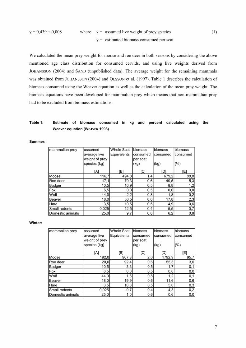
We calculated the mean prey weight for moose and roe deer in both seasons by considering the above

mentioned age class distribution for consumed cervids, and using live weights derived from

JOHANSSON (2004) and SAND (unpublished data). The average weight for the remaining mammals

was obtained from JOHANSSON (2004) and OLSSON et al. (1997). Table 1 describes the calculation of

biomass consumed using the Weaver equation as well as the calculation of the mean prey weight. The

biomass equations have been developed for mammalian prey which means that non-mammalian prey

had to be excluded from biomass estimations.

Table 1: Estimate of biomass consumed in kg and percent calculated using the….. Weaver equation (WEAVER 1993).

Summer:

Winter:

mammalian prey assumed average live weight of prey species (kg)

Whole ScatEquivalents

biomass consumed per scat(kg)

biomass consumed (kg)

biomass consumed (%)

[A] [B] [C] [D] [E]Moose 116,7 494,8 1,4 679,2 88,8Roe deer 17,1 70,3 0,6 40,5 5,3Badger 10,5 16,9 0,5 8,8 1,2Fox 6,5 0,0 0,5 0,0 0,0Wolf 44,0 2,2 0,8 1,8 0,2Beaver 18,0 30,5 0,6 17,8 2,3Hare 3,5 10,5 0,5 4,9 0,6Small rodents 0,025 12,5 0,4 5,5 0,7Domestic animals 25,0 9,7 0,6 6,2 0,8

mammalian prey assumed average live weight of prey species (kg)

Whole ScatEquivalents

biomass consumed per scat(kg)

biomass consumed

(kg)

biomass consumed

(%)

[A] [B] [C] [D] [E]Moose 192,0 907,8 2,0 1792,9 95,7Roe deer 20,0 92,4 0,6 55,3 3,0Badger 10,5 3,3 0,5 1,7 0,1Fox 6,5 0,0 0,5 0,0 0,0Wolf 44,0 1,5 0,8 1,2 0,1Beaver 18,0 19,9 0,6 11,6 0,6Hare 3,5 10,8 0,5 5,0 0,3Small rodents 0,025 9,7 0,4 4,3 0,2Domestic animals 25,0 1,0 0,6 0,6 0,0

7

Table 1: (continued) Estimate of biomass consumed in kg and percent calculated using the….. Weaver equation (WEAVER 1993).

[A] Moose (summer): average weight calculated as follows: (0,8*78,4 kg)+(0,1*220 kg)+(0,1*320 kg) Moose (winter): average weight calculated as follows: (0,8*160 kg)+(0,1*290 kg)+(0,1*350 kg)resulting from calf:yearling:adult = 80:10:10 (nach SAND unpubl. data, PEDERSEN et al. 2005); average weights for certain age groups derived from JOHANSSON (2004) and SAND (unpubl. Data);

Roe deer (summer): (0,5*9,3 kg)+(0,5*25 kg) resulting from Juvenile:Adult = 1:1 (JOHANSSON 2004);average weights for certain age groups derived from JOHANSSON (2004) and SAND (unpubl. Data);Roe deer (winter): 20 kg; average weight for all age groups (SAND unpubl. data)

Badger, Beaver, Hare (JOHANSSON 2004)Wolf (SAND 2005)small rodents (OLSSON et al. 1997)Domestic animals (derived from OLSSON et al. 1997)

[B] WSE [C] calculated using the Weaver equation (WEAVER 1993): y = 0,439 + 0,008x

x = assumed live weight of prey species (see [A]); y = estimated biomass consumed per scat (kg);

[D] B * C [E] D / Σ D

To compare the conventional methods for biomass calculations, we also applied the equations

developed by FLOYD et al. (1978) (2) and RÜHE (unpublished, derived from table 1 in RÜHE et al.

2003) (3):

y = 0,383 + 0,02 (Floyd equation) (2)

y = 0,0731 + 0,00406 (Rühe equation) (3)

To investigate if wolves in Scandinavia prefer one of the two cervid species, Manly’s Alpha

preference index was calculated:

( )∑=

jji

ii nrn

r/

1α where αi =

Manly’s Alpha (preference index) for prey

type i

(4)

ri, rj = Proportion of prey type i or j in the diet

ni, nj = Proportion of prey type i or j in the

environment

8

Selective feeding does not occur, if αi = 1/m (m = total number of prey types). Prey species i is

preferred if αi is greater than 1/m, whereas negative selection is found if αi is less than 1/m.

Levin’s Food Niche Breadth (FNB) was used to measure specialization quantitatively for the diet

composition of wolves on the Scandinavian peninsula:

∑= 2

1

jpB where B = Levin’s Food Niche Breadth (5)

pj = Proportion of fractions of items in the diet that are

of food category j

Levin’s Food Niche Breadth can be standardized and expressed in a scale from 0 to 1 with the help of

equation (6), whereat 0 represents high specialisation and 1 stands for equal use of all prey items.

11

−−

=nBBA where BA = Levin’s standardized Food Niche Breadth (6)

B = Levin’s Food Niche Breadth

n = Number of possible resource states

Statistical analyses

The data was analysed using SPSS version 13.0 and 14.0 as well as StatView. We compared diet

composition among the two seasons based on absolute frequency of occurrence with which individual

prey items occurred in the sample. The analyses were conducted by using 2x2 contingency table

analysis at a significance level of p = 0.05. We used linear regression analysis to investigate the

relationship between population densities and FNB. Pellet group counts to quantify population

densities were carried out in springtime, hence we assumed that the densities were on an equal level in

summer and winter. To compare FNB between summer and winter, data pairs consisting of different

territories were analysed using Wilcoxon signed ranks test.

9

4 Results

Diet composition on the Scandinavian peninsula

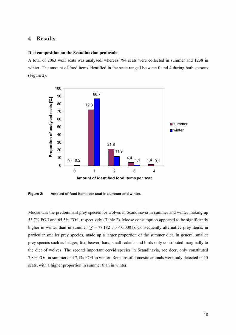
A total of 2063 wolf scats was analysed, whereas 794 scats were collected in summer and 1238 in

winter. The amount of food items identified in the scats ranged between 0 and 4 during both seasons

(Figure 2).

Figure 2: Amount of food items per scat in summer and winter.

21,8

86,7

0,1 1,44,4

72,3

0,2 0,11,1

11,9

0

10

20

30

40

50

60

70

80

90

100

0 1 2 3 4

Amount of identified food items per scat

Prop

ortio

n of

ana

lyse

d sc

ats

[%]

summerwinter

Moose was the predominant prey species for wolves in Scandinavia in summer and winter making up

53,7% FO/I and 65,5% FO/I, respectively (Table 2). Moose consumption appeared to be significantly

higher in winter than in summer (χ2 = 77,182 ; p < 0,0001). Consequently alternative prey items, in

particular smaller prey species, made up a larger proportion of the summer diet. In general smaller

prey species such as badger, fox, beaver, hare, small rodents and birds only contributed marginally to

the diet of wolves. The second important cervid species in Scandinavia, roe deer, only constituted

7,8% FO/I in summer and 7,1% FO/I in winter. Remains of domestic animals were only detected in 15

scats, with a higher proportion in summer than in winter.

10

11

0

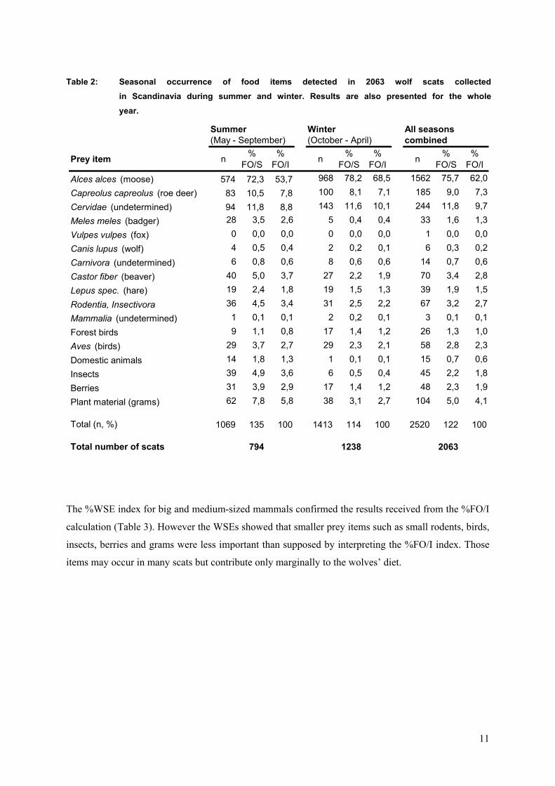
Table 2: Seasonal occurrence of food items detected in 2063 wolf scats collectedin Scandinavia during summer and winter. Results are also presented for the wholeyear.

Summer Winter All seasons (May - September) (October - April) combined

Prey item n % FO/S

% FO/I n %

FO/S%

FO/I n % FO/S

% FO/I

Alces alces (moose) 574 72,3 53,7 968 78,2 68,5 1562 75,7 62,0

Capreolus capreolus (roe deer) 83 10,5 7,8 100 8,1 7,1 185 9,0 7,3

Cervidae (undetermined) 94 11,8 8,8 143 11,6 10,1 244 11,8 9,7

Meles meles (badger) 28 3,5 2,6 5 0,4 0,4 33 1,6 1,3

Vulpes vulpes (fox) 0 0,0 0,0 0 0,0 0,0 1 0,0 0,0Canis lupus (wolf) 4 0,5 0,4 2 0,2 0,1 6 0,3 0,2

Carnivora (undetermined) 6 0,8 0,6 8 0,6 0,6 14 0,7 0,6

Castor fiber (beaver) 40 5,0 3,7 27 2,2 1,9 70 3,4 2,8Lepus spec. (hare) 19 2,4 1,8 19 1,5 1,3 39 1,9 1,5

Rodentia, Insectivora 36 4,5 3,4 31 2,5 2,2 67 3,2 2,7

Mammalia (undetermined) 1 0,1 0,1 2 0,2 0,1 3 0,1 0,1

Forest birds 9 1,1 0,8 17 1,4 1,2 26 1,3 1,

Aves (birds) 29 3,7 2,7 29 2,3 2,1 58 2,8 2,3

Domestic animals 14 1,8 1,3 1 0,1 0,1 15 0,7 0,6

Insects 39 4,9 3,6 6 0,5 0,4 45 2,2 1,8

Berries 31 3,9 2,9 17 1,4 1,2 48 2,3 1,9

Plant material (grams) 62 7,8 5,8 38 3,1 2,7 104 5,0 4,1

Total (n, %) 1069 135 100 1413 114 100 2520 122 100

Total number of scats 794 1238 2063

The %WSE index for big and medium-sized mammals confirmed the results received from the %FO/I

calculation (Table 3). However the WSEs showed that smaller prey items such as small rodents, birds,

insects, berries and grams were less important than supposed by interpreting the %FO/I index. Those

items may occur in many scats but contribute only marginally to the wolves’ diet.

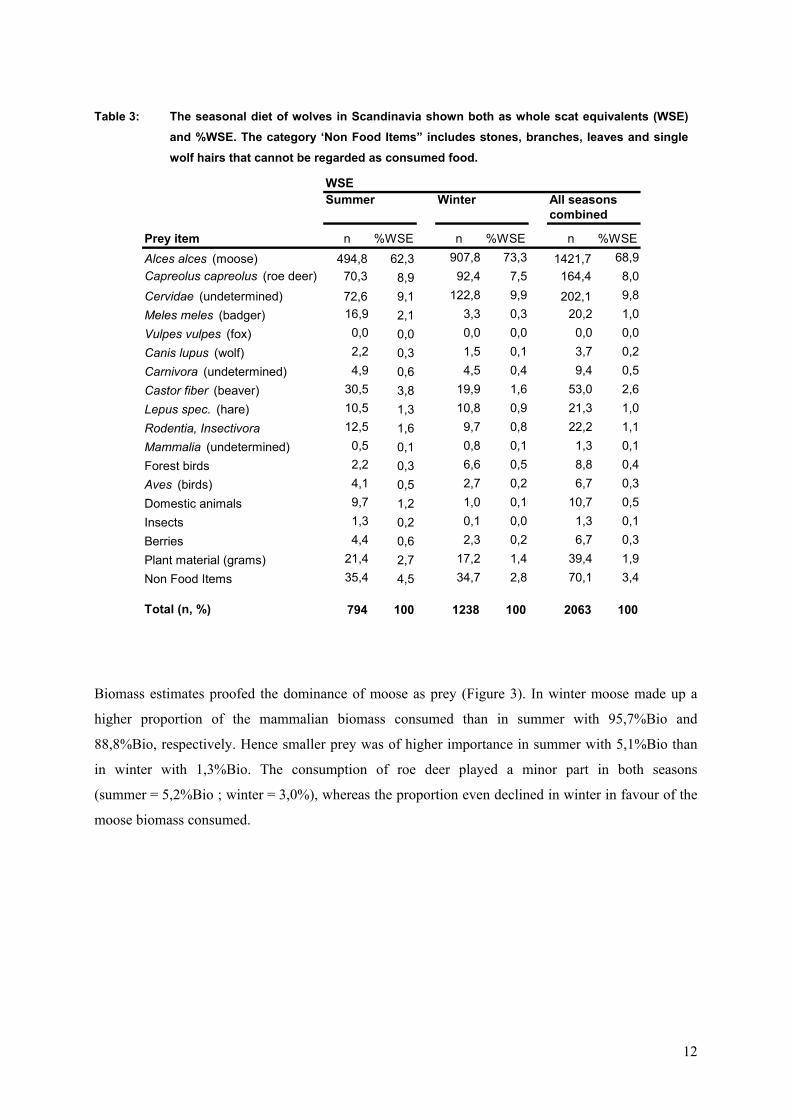
Table 3: The seasonal diet of wolves in Scandinavia shown both as whole scat equivalents (WSE) and %WSE. The category ‘Non Food Items” includes stones, branches, leaves and single wolf hairs that cannot be regarded as consumed food.

WSESummer Winter All seasons

combined

Prey item n %WSE n %WSE n %WSEAlces alces (moose) 494,8 62,3 907,8 73,3 1421,7 68,9Capreolus capreolus (roe deer) 70,3 8,9 92,4 7,5 164,4 8,0Cervidae (undetermined) 72,6 9,1 122,8 9,9 202,1 9,8Meles meles (badger) 16,9 2,1 3,3 0,3 20,2 1,0Vulpes vulpes (fox) 0,0 0,0 0,0 0,0 0,0 0Canis lupus (wolf) 2,2 0,3 1,5 0,1 3,7 0Carnivora (undetermined) 4,9 0,6 4,5 0,4 9,4 0Castor fiber (beaver) 30,5 3,8 19,9 1,6 53,0 2,6Lepus spec. (hare) 10,5 1,3 10,8 0,9 21,3 1,0Rodentia, Insectivora 12,5 1,6 9,7 0,8 22,2 1,1Mammalia (undetermined) 0,5 0,1 0,8 0,1 1,3 0Forest birds 2,2 0,3 6,6 0,5 8,8 0Aves (birds) 4,1 0,5 2,7 0,2 6,7 0Domestic animals 9,7 1,2 1,0 0,1 10,7 0,5Insects 1,3 0,2 0,1 0,0 1,3 0Berries 4,4 0,6 2,3 0,2 6,7 0Plant material (grams) 21,4 2,7 17,2 1,4 39,4 1,9Non Food Items 35,4 4,5 34,7 2,8 70,1 3,4

Total (n, %) 794 100 1238 100 2063 100

,0,2,5

,1,4,3

,1,3

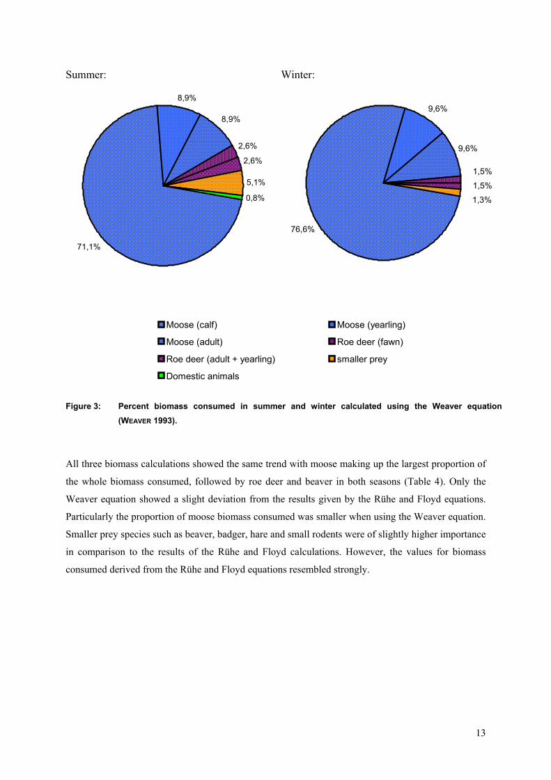
Biomass estimates proofed the dominance of moose as prey (Figure 3). In winter moose made up a

higher proportion of the mammalian biomass consumed than in summer with 95,7%Bio and

88,8%Bio, respectively. Hence smaller prey was of higher importance in summer with 5,1%Bio than

in winter with 1,3%Bio. The consumption of roe deer played a minor part in both seasons

(summer = 5,2%Bio ; winter = 3,0%), whereas the proportion even declined in winter in favour of the

moose biomass consumed.

12

13

R 1993).

Summer: Winter:

Figure 3: Percent biomass consumed in summer and winter calculated using the Weaver equation (WEAVE

71,1%

8,9%

8,9%

2,6%

2,6%

5,1%

0,8%

76,6%

9,6%

9,6%

1,5%

1,5%

1,3%

Moose (calf) Moose (yearling)

Moose (adult) Roe deer (fawn)

Roe deer (adult + yearling) smaller prey

Domestic animals

All three biomass calculations showed the same trend with moose making up the largest proportion of

the whole biomass consumed, followed by roe deer and beaver in both seasons (Table 4). Only the

Weaver equation showed a slight deviation from the results given by the Rühe and Floyd equations.

Particularly the proportion of moose biomass consumed was smaller when using the Weaver equation.

Smaller prey species such as beaver, badger, hare and small rodents were of slightly higher importance

in comparison to the results of the Rühe and Floyd calculations. However, the values for biomass

consumed derived from the Rühe and Floyd equations resembled strongly.

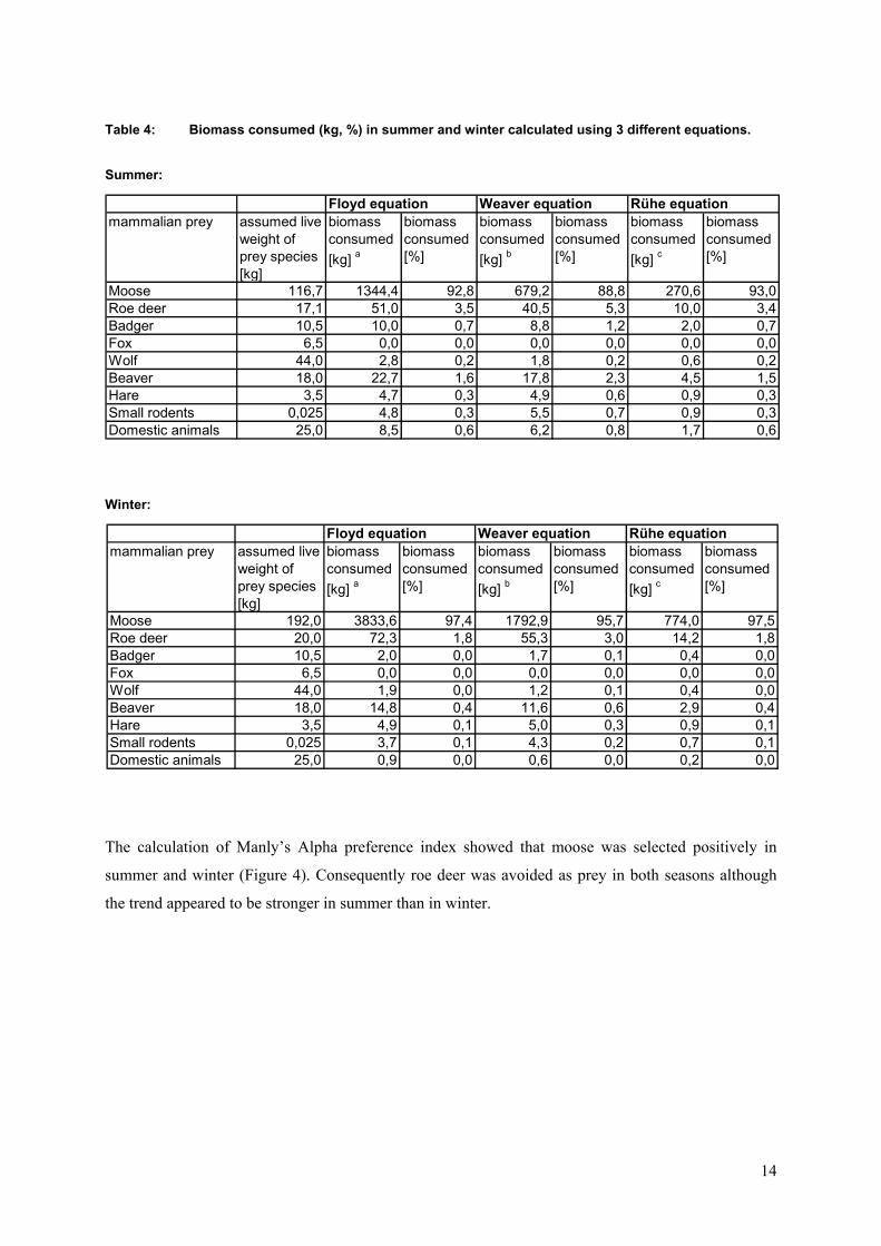
Table 4: Biomass consumed (kg, %) in summer and winter calculated using 3 different equations.

Summer:

Winter:

Floyd equation Weaver equation Rühe equationmammalian prey assumed live

weight of prey species [kg]

biomass consumed[kg] a

biomass consumed[%]

biomass consumed[kg] b

biomass consumed[%]

biomass consumed[kg] c

biomass consumed[%]

Moose 116,7 1344,4 92,8 679,2 88,8 270,6 93,0Roe deer 17,1 51,0 3,5 40,5 5,3 10,0 3,4Badger 10,5 10,0 0,7 8,8 1,2 2,0 0,7Fox 6,5 0,0 0,0 0,0 0,0 0,0 0,0Wolf 44,0 2,8 0,2 1,8 0,2 0,6 0,2Beaver 18,0 22,7 1,6 17,8 2,3 4,5 1,5Hare 3,5 4,7 0,3 4,9 0,6 0,9 0,3Small rodents 0,025 4,8 0,3 5,5 0,7 0,9 0,3Domestic animals 25,0 8,5 0,6 6,2 0,8 1,7 0,6

Floyd equation Weaver equation Rühe equationmammalian prey assumed live

weight of prey species [kg]

biomass consumed[kg] a

biomass consumed[%]

biomass consumed[kg] b

biomass consumed[%]

biomass consumed[kg] c

biomass consumed[%]

Moose 192,0 3833,6 97,4 1792,9 95,7 774,0 97,5Roe deer 20,0 72,3 1,8 55,3 3,0 14,2 1,8Badger 10,5 2,0 0,0 1,7 0,1 0,4 0,0Fox 6,5 0,0 0,0 0,0 0,0 0,0 0,0Wolf 44,0 1,9 0,0 1,2 0,1 0,4 0,0Beaver 18,0 14,8 0,4 11,6 0,6 2,9 0,4Hare 3,5 4,9 0,1 5,0 0,3 0,9 0,1Small rodents 0,025 3,7 0,1 4,3 0,2 0,7 0,1Domestic animals 25,0 0,9 0,0 0,6 0,0 0,2 0,0

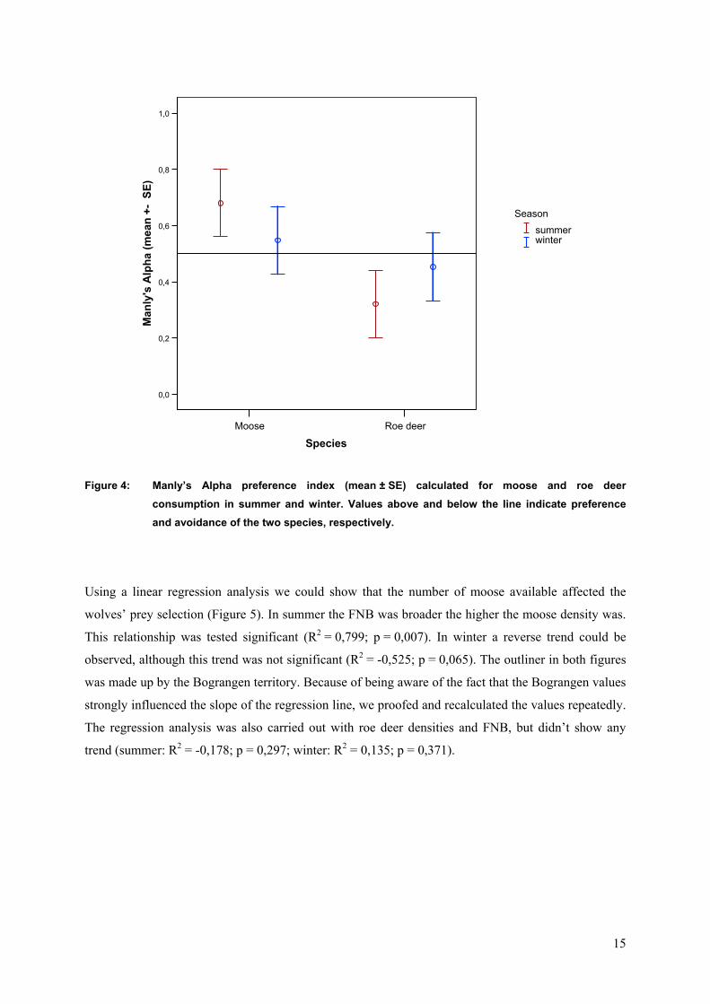
The calculation of Manly’s Alpha preference index showed that moose was selected positively in

summer and winter (Figure 4). Consequently roe deer was avoided as prey in both seasons although

the trend appeared to be stronger in summer than in winter.

14

Roe deerMoose

Species

1,0

0,8

0,6

0,4

0,2

0,0

Man

ly's

Alp

ha (m

ean

+- S

E)

21

Seasonsummer winter

Figure 4: Manly’s Alpha preference index (mean ± SE) calculated for moose and roe deer consumption in summer and winter. Values above and below the line indicate preference and avoidance of the two species, respectively.

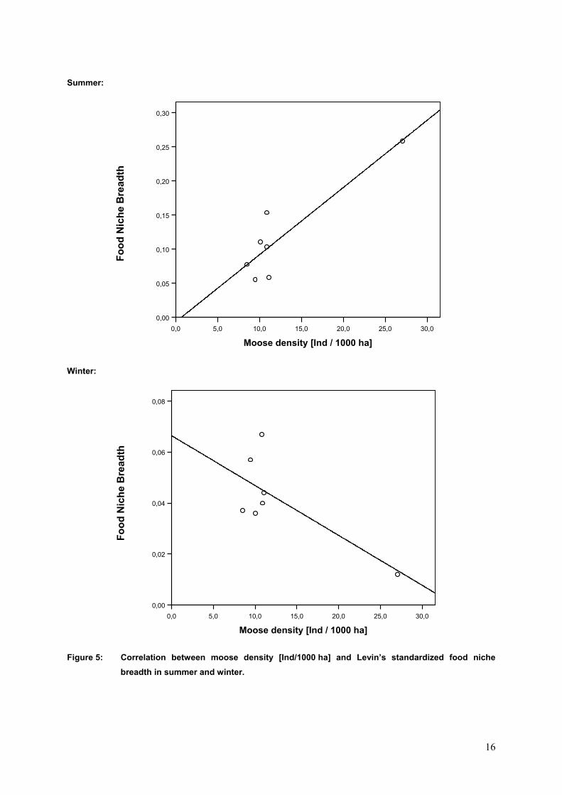
Using a linear regression analysis we could show that the number of moose available affected the

wolves’ prey selection (Figure 5). In summer the FNB was broader the higher the moose density was.

This relationship was tested significant (R2 = 0,799; p = 0,007). In winter a reverse trend could be

observed, although this trend was not significant (R2 = -0,525; p = 0,065). The outliner in both figures

was made up by the Bograngen territory. Because of being aware of the fact that the Bograngen values

strongly influenced the slope of the regression line, we proofed and recalculated the values repeatedly.

The regression analysis was also carried out with roe deer densities and FNB, but didn’t show any

trend (summer: R2 = -0,178; p = 0,297; winter: R2 = 0,135; p = 0,371).

15

16

d winter.

Summer:

Winter:

Figure 5: Correlation between moose density [Ind/1000 ha] and Levin’s standardized food niche breadth in summer an

30,025,020,015,010,05,00,0

Moose density [Ind / 1000 ha]

0,30

0,25

0,20

0,15

0,10

0,05

0,00

Food

Nic

he B

read

th

30,025,020,015,010,05,00,0

Moose density [Ind / 1000 ha]

0,08

0,06

0,04

0,02

0,00

Food

Nic

he B

read

th

0

20

40

60

80

100

Moose

Roe de

er

Cervid

Beave

rHare

S/Rod

Birds

Plants

Other

0

20

40

60

80

100

Moose

Roe de

er

Cervid

Beave

rHare

S/Rod

Birds

Plants

Other

Bograngen Dals-Ed

Filipstad Grangärde

Hagfors Hasselfors

0

20

40

60

80

100

Moose

Roe de

er

Cervid

Beave

rHare

S/Rod

Birds

Plants

Other

0

20

40

60

80

100

Moose

Roe de

er

Cervid

Beave

rHare

S/Rod

Birds

Plants

Other

0

20

40

60

80

100

Moose

Roe de

er

Cervid

Beave

rHare

S/Rod

Birds

Plants

Other

0

20

40

60

80

100

Moose

Roe de

er

Cervid

Beave

rHare

S/Rod

Birds

Plants

Other

17

0

20

40

60

80

100

Moose

Roe de

er

Cervid

Beave

rHare

S/Rod

Birds

Plants

Other

0

20

40

60

80

100

Moose

Roe de

er

Cervid

Beave

rHare

S/Rod

Birds

Plants

Other

Leksand Nyskoga

Tisjön Tyngsjö

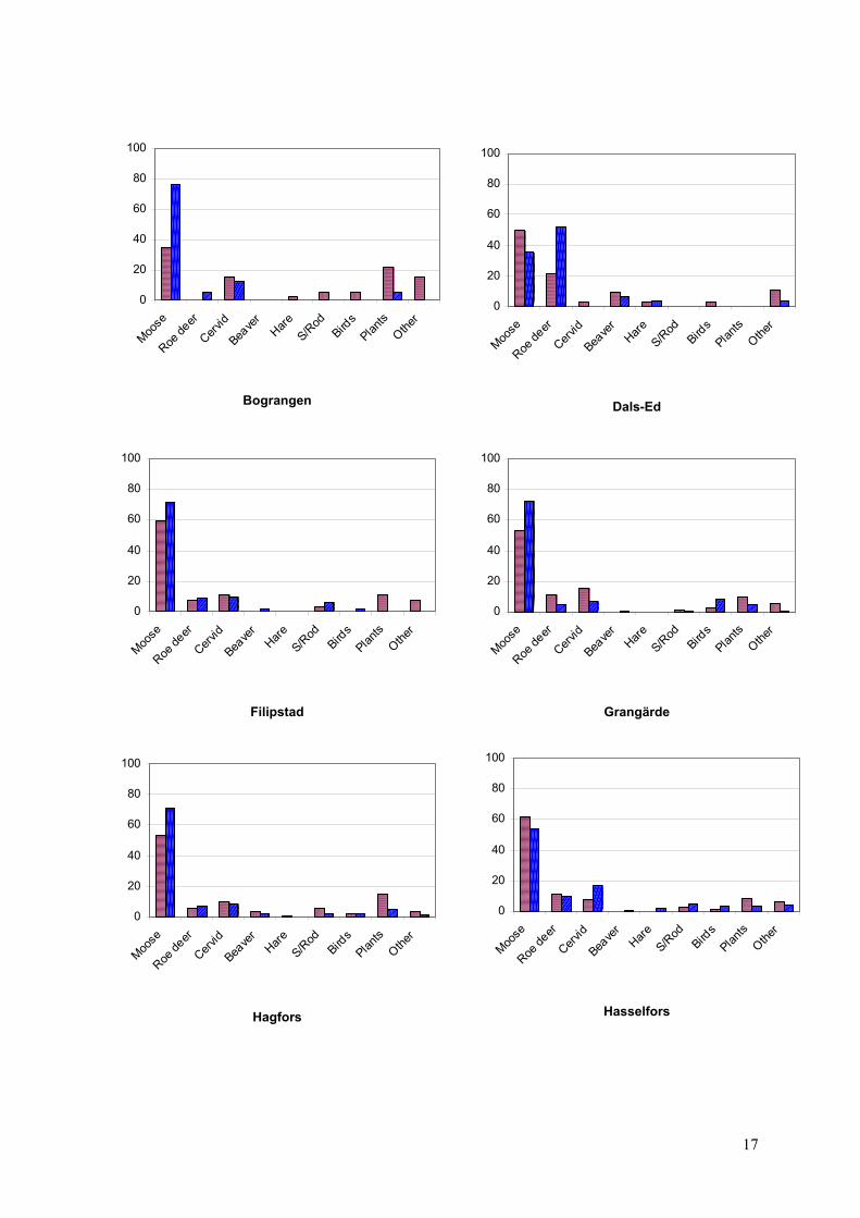
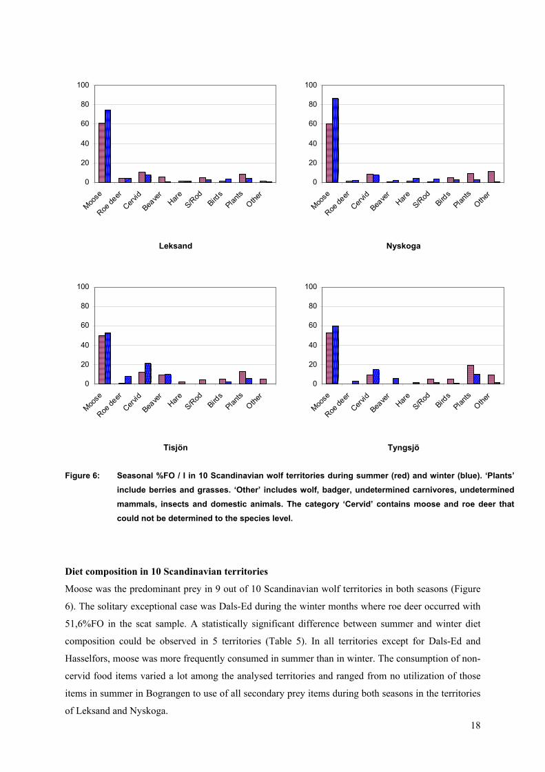
Figure 6: Seasonal %FO / I in 10 Scandinavian wolf territories during summer (red) and winter (blue). ‘Plants’ include berries and grasses. ‘Other’ includes wolf, badger, undetermined carnivores, undetermined mammals, insects and domestic animals. The category ‘Cervid’ contains moose and roe deer that could not be determined to the species level.

0

20

40

60

80

100

Moose

Roe de

er

Cervid

Beave

rHare

S/Rod

Birds

Plants

Other

0

20

40

60

80

100

Moose

Roe de

er

Cervid

Beave

rHare

S/Rod

Birds

Plants

Other

Diet composition in 10 Scandinavian territories

Moose was the predominant prey in 9 out of 10 Scandinavian wolf territories in both seasons (Figure

6). The solitary exceptional case was Dals-Ed during the winter months where roe deer occurred with

51,6%FO in the scat sample. A statistically significant difference between summer and winter diet

composition could be observed in 5 territories (Table 5). In all territories except for Dals-Ed and

Hasselfors, moose was more frequently consumed in summer than in winter. The consumption of non-

cervid food items varied a lot among the analysed territories and ranged from no utilization of those

18

items in summer in Bograngen to use of all secondary prey items during both seasons in the territories

of Leksand and Nyskoga.

19

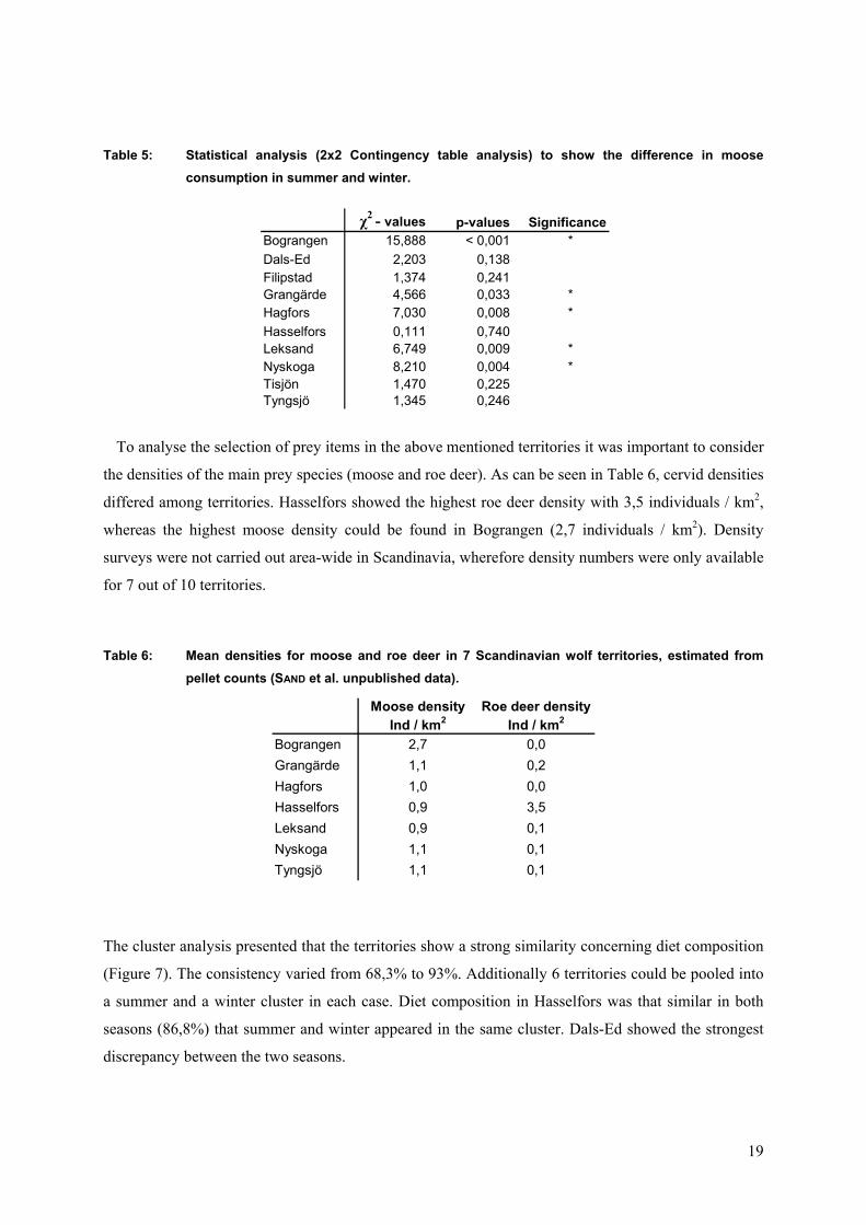
able 5: Statistical analysis (2x2 Contingency table analysis) to show the difference in moose consumption in summer and winter.

To analyse the selection of portant to consider

e densities of the main prey species (moose and roe deer). As can be seen in Table 6, cervid densities

d

T le 6: Mean densities for moose and roe deer in 7 Scandinavian wolf territories, estimated from pellet counts (SAND et al. unpublished data).

he cluster analysis presented that the territories show a strong similarity concerning diet composition

igure 7). The consistency varied from 68,3% to 93%. Additionally 6 territories could be pooled into

Ind / km0,0

T

χ2 - values p-values Significance

Bograngen 15,888 < 0,001 *Dals-Ed 2,203 0,138Filipstad 1,374 0,241Grangärde 4,566 0,033 *Hagfors 7,030 0,008 *Hasselfors 0,111 0,740Leksand 6,749 0,009 *Nyskoga 8,210 0,004 *Tisjön 1,470 0,225Tyngsjö 1,345 0,246

prey items in the above mentioned territories it was im

th

iffered among territories. Hasselfors showed the highest roe deer density with 3,5 individuals / km2,

whereas the highest moose density could be found in Bograngen (2,7 individuals / km2). Density

surveys were not carried out area-wide in Scandinavia, wherefore density numbers were only available

for 7 out of 10 territories.

ab

Moose density Roe deer densityInd / km2 2

Bograngen 2,7Grangärde 1,1 0,2Hagfors 1,0 0,0Hasselfors 0,9 3,5Leksand 0,9 0,1Nyskoga 1,1 0,1Tyngsjö 1,1 0,1

T

(F

a summer and a winter cluster in each case. Diet composition in Hasselfors was that similar in both

seasons (86,8%) that summer and winter appeared in the same cluster. Dals-Ed showed the strongest

discrepancy between the two seasons.

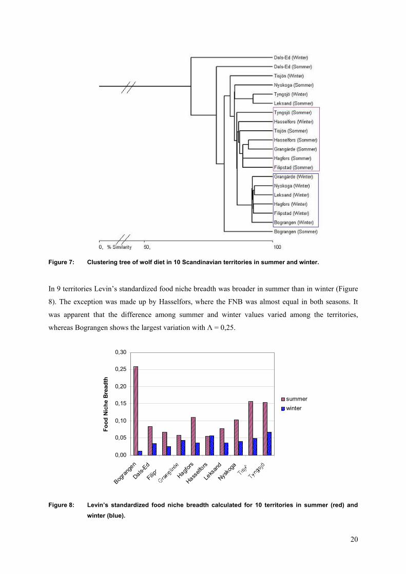
Figure 7: Clustering tree of wolf diet in 10 Scandinavian territories in summer and winter.

In 9 territories Levin’s standardized food niche breadth was broader in summer than in winter (Figure

8). The exception was made up by Hasselfors, where the FNB was almost equal in both seasons. It

was apparent that the difference among summer and winter values varied among the territories,

whereas Bograngen shows the largest variation with Λ = 0,25.

Figure 8: Levin’s standardized food niche breadth calculated for 10 territories in summer (red) and winter (blue).

0,00

0,05

0,10

0,15

0,20

0,25

0,30

Bogran

gen

Dals-Ed

Filipsta

d

Hagfors

Hasself

ors

Leks

and

Nysko

ga

Food

Nic

he B

read

th

summerwinter

20

21

5 Discussion

Seasonal diet composition in Scandinavia

In the course of this study we could verify that moose is by far the most important prey species for

wolves in Scandinavia, both by frequency of occurrence and biomass consumed. Numerous studies on

wolf diet affirm that wild ungulates and in particular large ungulates make up the main part of the diet

composition (FRENZEL 1974, VOIGT et al. 1976, MATTIOLI et al. 1995, MERRIGI et al. 1996, GADE-

JØRGENSEN & STAGEGAARD 2000, JEDRZEJEWSKI et al. 2000, CAPITANI et al. 2004, SMIETANA 2005,

ANSORGE et al. 2006). Nevertheless secondary and smaller prey items such as beaver, hare, small

rodents, and berries can be of seasonal importance (FRENZEL 1974, MECH & BOITANI 2003). The

significant difference between the diet composition among summer and winter in our study area is

mainly based on the increased use of those secondary prey items during the summer months. This

trend might be explained by the abundance and higher activity of smaller prey species in summer

(JOHANSSON 2004). Accordingly the importance of moose even increased during the winter months,

what might be explained by the effort to earn maximum benefit with minimum costs. LEŚNIEWICZ &

PERZANOWSKI (1989) describe that wolves tend to concentrate on large ungulates during winter time

to maximize the gained food biomass per successful hunt and therefore prefer larger prey species.

In contrast to a previous study on foraging behaviour of wolves in Scandinavia based on scat

analysis carried out by OLSSON et al. (1997), roe deer only contributes marginally to the wolves’ diet

with a slightly higher importance in summer than in winter. OLSSON et al. (1997) describe that the

Scandinavian wolves prey on roe deer with 51 %FO/S in summer and 47 %FO/S in winter, whereas in

the current study roe deer constitutes 10,5 %FO/S in summer and 8,1 %FO/S in winter. There are

many explanations for the evident differences between our study and the results described by OLSSON

et al. (1997). OLSSON et al. (1997) conducted their study in the Nyskoga territory from 1988 to 1992,

whereas our data was collected in almost all Scandinavian territories from 1992 to 2005. Additionally

the size of the dataset differs strongly (OLSSON et al. 1997: n = 684; current study: n = 2063). Another

explanation for the different results and the high utilization of roe deer from 1988 to 1992 might be the

increase in roe deer numbers that was reported in the early 90s, followed by a decrease in the

population density in subsequent years (SVENSKA JÄGAREFÖRBUNDET 2005).

Although roe deer appears frequently in the diet of wolves within its range in Europe (SALVADOR &

ABAD 1987, MATTIOLI et al. 1995, JEDRZEJEWSKI et al. 2000, SIDOROVICH et al. 2003, MATTIOLI et

al. 2004, GAZZOLA et al. 2005, NOWAK et al. 2005, ANSORGE et al. 2006), it rarely constitutes the

main food resource (VALDMANN et al. 1998, GAZZOLA et al. 2005, ANSORGE et al. 2006). AANES et

al. (1998) describe this trend with the small amount of biomass that roe deer offers in comparison to

red deer or moose. Therefore roe deer appears to be of comparatively inferior quality in view of

effective foraging. Particularly in agricultural and non-forested areas the importance of roe deer as

22

prey increases due to higher population densities and the fact that roe deer is easier to prey on under

those circumstances (LINNELL & ANDERSEN 1995, MATTIOLI et al. 2004, ANSORGE et al. 2006).

We observed a relatively high occurrence of plant material, in particular grams, in the analysed scats

both in summer and winter. The consumption of grams is supposed to be effective as a purgative and

to wipe the intestine from parasites and hairs (MECH & BOITANI 2003). Both grams and berries were

consumed more frequently in summer than in winter due to the higher availability of plants during the

summer months. Although we assume that grams are partly consumed by chance in consequence of

the feeding behaviour of wolves and the habit to lick blood from the ground, grams that appear in

well-ordered bundles and with more than 5% of the dry volume of the scat need to be regarded as

voluntarily consumed.

Even though the annual number of wolf-killed domestic animals in Sweden is quoted with about 200

individuals, this potential prey only contributed marginally to the diet of wolves within our study. 95%

of the killed domestic animals in Sweden are sheep (SWEDISH WILDLIFE DAMAGE CENTRE 2004).

Detailed numbers for Norway are not known, but it is assumed that 200-400 sheep are killed per year.

We identified hairs of sheep (n = 12), pigs (n = 2) and dogs (n = 1) in 14 summer scats and 1 winter

scat (Table 2). The only winter scat that contained remains of a domestic animal was collected in

Nyskoga and included sheep hairs. The remaining domestic animal items were observed in summer

scats collected in Norwegian territories (Rømskog: n = 2; Våler: n = 10), in Dals-Ed that is located in

the Norwegian-Swedish border country (n = 1) and Grangärde (n = 1) in Sweden. The seasonal

variation in the consumption of domestic animals can be explained by the fact that sheep are only

found on pastures or free-grazing during the summer months (LIBERG 2006).

The remains of domestic animals only occurred in a few scats. Nevertheless it is obvious that the

predation on e.g. sheep is a bigger problem in Norway than in Sweden. Apparently this results from

the way of sheep farming in Norway: about 2.1 million sheep range free on large parts of the country

and provide an easy meal for predators.

In northern and central Europe, domestic animals do not make up an important part of the wolves’

diet (OLSSON et al. 1997, GADE-JØRGENSEN & STAGEGAARD 2000, ANSORGE et al. 2006), whereas

wolves in southern and eastern Europe prey on domestic animals to a much higher extend. Remains of

domestic animals are detected with 2,3%FO/I to 95,5%FO/I (derived from BIBIKOV et al. 1985 in

OKARMA 1995, SALVADOR & ABAD 1987, MATTIOLI et al. 1995, VOS 2000, CAPITANI et al. 2004,

GAZZOLA et al. 2005, NOWAK et al. 2005). The consumption of domestic animals appears to be

highest in areas where wild ungulates are rare (MERRIGI & LOVARI 1996, VOS 2000). In areas, where

wild and domestic ungulates coexist, wild ungulates constitute the preferred prey (GAZZOLA et al.

2005, ANSORGE et al. 2006).

23

Prey selection

Our study showed that moose is the preferred cervid species on the Scandinavian peninsula, both in

summer and winter. This result contrasts with the statement by MECH (1970), POTVIN et al. (1988),

SPAULDING et al. (1998) und TREMBLAY et al. (2001) that wolves prefer the species that is smaller or

easier to catch if there are 2 or more cervid species available. On an intra specific level this statement

applies to the Scandinavian wolf population, since 80% of all moose killed are calves (PEDERSEN et al.

2005, SAND unpublished data). Concerning the selection of moose and roe deer we seem to face a

different situation in Scandinavia. KUNKEL et al. (2004) argue that the selection of prey takes place on

two levels. Wolves select prey that is easiest to locate and that provides the largest amount of biomass

per successful attack. Both criterions fit for moose in Scandinavia due to the comparatively high

population density (0,6 – 2,5 individuals per km2, SAND 2005) and the high biomass per individual

(78kg – 350kg, JOHANSSON 2004, SAND unpublished data). Anyhow large prey species and in

particular moose are dangerous to attack and a wolf might get injured or even killed when attacking a

moose (WEAVER et al. 1992). Nevertheless moose seem to be an easy prey for wolves in Scandinavia.

SAND et al. (2006) state that moose in Scandinavia are currently naive to wolves due to the missing

and low predation pressure when wolves were extinct on the Scandinavian peninsula in the 1960s and

slowly expanded again in the 1980s. The long period of separation of moose and wolves in

Scandinavia apparently caused a loss of an effective anti-predator behaviour, which needs to be

regained now. Because of their inexperience with large carnivores moose on the Scandinavian

peninsula are more vulnerable to wolf attacks than moose in North America (SAND et al.2006).

Another reason for the preference of moose and the avoidance of roe deer in summer and winter

might be the coexistence of wolves with lynx in Scandinavia. MOSHØJ (XXXX) in Sweden and SUNDE

et al. (2000) in Norway describe that roe deer is an important prey for lynx. Hence the prey selection

by wolves might also be explained by food niche separation

Food Niche Breadth

Standardized Food Niche Breadth was relatively low in both seasons (summer: BA = 0,11; winter:

BA = 0,04) what indicates a specialisation on one prey category. In our study the diet of wolves was

dominated by cervids. Moreover Food Niche Breadth in summer was significantly broader than in

winter. This trend was caused by the higher availability and utilization of alternative prey species such

as beaver, hare, small rodents and birds.

MERRIGI et al. (1996) stated in their study that the Food Niche Breadth is influenced by the density

of large ungulates. They described that wolves specialise on large ungulates if those prey species are

available in high numbers. Therefore the density of the main prey species has an influence on the Food

Niche Breadth. Our results follow this trend in both seasons. In accordance to MERRIGI et al. (1996)

the standardized Food Niche Breadth in winter decreases with increasing moose density. That means

that in winter wolves in Scandinavia concentrate even more on moose if their density is high.

24

Consequently during winter time the wolves seem to prefer the prey category whose availability is

highest (HAYES et al. 2000). In contrast to the results in winter, a reverse trend could be documented

in summer. The standardized Food Niche Breadth increases with raising moose numbers. An

explanation for this trend could be that the wolves adapt their foraging behaviour in summer to the

given prey diversity. It is possible that the wolves supplement their summer diet with alternative prey

items, although the preferred prey is available in high numbers (THEBERGE & COTTRELL 1977,

THEBERGE et al. 1978, FORBES & THEBERGE 1996, TREMBLAY et al. 2001).

Diet composition in 10 Scandinavian territories

In general the diet composition in the Scandinavian wolf territories appears to be very similar (Figure

7). Differences among territories within the same season can be explained by varying availability and

vulnerability of prey species as well as varying a biotic factors (e.g. snow depth, landscape

management, clear cutting, road density). Additionally we described that always 6 territories can be

pooled in summer and winter clusters, respectively. Therefore we assume that the similarities among

the territories are mainly caused by the seasonal availability of given food resources.

Bograngen and Dals-Ed show the highest deviations between summer and winter diet. In Dals-Ed

the deviation mainly seems to be caused by the comparatively high roe deer consumption during the

winter months. However, this result needs to be handled carefully, since the seasonal differences may

also be caused by the varying sample size (summer: n = 57; winter: n = 29). The same applies to

Bograngen. The evident difference between summer and winter diet seems to be caused by the

concentration on cervids and in particular moose as prey during winter. It is possible that the wolves

indeed do not resort to secondary prey items because of the high availability of moose during winter.

Bograngen shows the highest moose density among the studied territories and is known as a winter

stand for moose (SAND unpublished data). Nevertheless we cannot exclude that the deviations also

result from a small sample size (summer: n = 23; winter: n = 36). Therefore it is necessary to carry out

further studies including a larger sample size as well as more extensive information about prey

densities, to make detailed predictions about the differences in the seasonal diet composition.

We could also show that Dals-Ed and Hasselfors are the only territories among the studied ones that

show higher moose consumption in summer than in winter. The remaining territories describe the

already discussed trend with a high concentration on moose as prey in winter and the more extensive

use of alternative prey in summer. Both Dals-Ed and Hasselfors are situated in areas with high roe

deer densities, however exact numbers are only available for Hasselfors. In our case it is possible that

due to the high availability of a second cervid species the wolves do not have to specialise on moose in

winter as they apparently do in the remaining territories. This trend is also reflected in the standardized

Food Niche Breadth in both seasons. MERRIGI et al. (2004) also argue that roe deer becomes more

attractive as prey in areas where it appears in high densities.

25

As a result we can assume that the preferences and the utilization of different prey items in the

studied territories were influenced by the prey densities as well as by the seasonal availability of food

items. Additionally the selection of certain prey is supposed to be a result of pack size and possible

reproductions in the territories (SPAULDING et al.1998, CAPITANI et al. 2004).

Calculation of biomass consumed

Within this study we compared 3 well-established methods used to calculate the biomass consumed by

carnivores. The differences between the 3 calculation methods are evident, but it is difficult to

evaluate them statistically. These deviations, in particular concerning large prey, result from the fact

that FLOYD et al. (1978), WEAVER (1993) and RÜHE (unpublished, derived from table 1 in RÜHE et al.

2003) took different prey species into account when establishing their equations. The largest prey

species that FLOYD et al. (1978) and RÜHE (unpublished, derived from table 1 in RÜHE et al. 2003)

integrated into their studies were white-tailed deer and red deer, respectively. Whereas WEAVER

(1993) considered elk and moose as well as the data from FLOYD et al. (1978) and TRAVES (1983).

Therefore the Weaver equation covers a higher variety of prey species and prey sizes than the other

two methods. The comparison between the 3 methods showed the importance of a sounded and a

crucial selection of the ‘right’ method when calculating the biomass consumed for a given study area.

Although RÜHE (unpublished, derived from table 1 in RÜHE et al. 2003) calculated his equation for

potential prey species in European ecosystems, it was more reasonable to chose the Weaver equation

in our study, because moose appeared to be the main prey for wolves in Scandinavia, and moose is

only integrated into the Weaver equation. By choosing the Weaver equation we did not overestimate

the moose biomass consumed as it would have been the case when choosing the Floyd or Rühe

equations.

Table 4 shows that the biomass consumed in kg also differs between the 3 methods. The values raise

from Rühe to Weaver to Floyd by factor 2. Those deviations result from the different methods Floyd,

Weaver and Rühe used when calculating the biomass equations: the amount of scats collected differed

as well as the number of wolves. Due to strong variation of biomass consumed in kg we cannot

recommend this kind of data presentation. Moreover, the biomass consumed in kg correlates with the

number of scats collected and never describes the biomass consumed for the whole wolf population.

Conclusions

Although we had an extensive dataset with 2063 scats, it appeared that the sample was not sufficient

for seasonal comparisons among territories. Only few territories provided enough scat samples per

season to integrate them into the data evaluation. For future studies we therefore recommend a

concentration of the data collection on only few territories with a sample size of at least 94 scats per

season (TRITES & JOY 2005). Additionally the data collection should cover a reasonable period, at

least 12 months. Considering these criterions, it is be possible to make detailed comparisons among

26

territories, seasons and years. Furthermore the availability of density data for the main prey species

should be crucial for the study area selection. In our study several territories could not be assessed and

compared in detail due to absent or deficient prey density data. Depending on the research question the

study focuses on, it appears to be practical to collect data in areas where density surveys were or will

be carried out.

However, when selecting the study area and study period one has to take into consideration that we

are dealing with an open system with fluctuating territories, and prey and predator densities.

Nevertheless it seems to be meaningful to concentrate on only a few territories and depending on the

research question to provide all the necessary biotic as well as a biotic extra information (e.g. prey

density, snow depth, road density).

Despite the above mentioned foibles, we were able to provide extensive and almost area-wide

information about the seasonal diet composition of wolves in Scandinavia. Since previous studies were

manly carried out during winter (PALM 2001, WIKENROS 2001, SAND et al. 2005, BERNELIND 2006,

SAND et al. in press), our study represents a good completion to the given dataset, in particular

concerning summer diet.

Generally a combination of scat analysis and carcass search provides a broader database, than both

methods individually: scat analysis gives overall information about the diet composition and detects

prey species that are not or hardly found by doing carcass search. Carcass search on the other hand

shows absolute numbers of animals killed and gives information about the carcass site. Hence scat

analysis is not a replacement for carcass search, but rather a supplementary method to get more

detailed information.

Résumé

• Moose was the dominant and preferred prey both in summer and winter.

• Secondary prey items such as beaver, hare and small rodents were more frequently used in

summer.

• Seasonal differences in the diet composition were given and mainly influenced by the

utilization of moose and smaller prey species.

• Food Niche Breadth was relatively narrow in both seasons which is explained by the high

concentration on cervids as prey. The even higher utilization of moose during the winter

months resulted into a lower Food Niche Breadth in winter than in summer.

• The moose density in the Scandinavian territories had an influence on the selection of moose

as prey and therefore also on the Food Niche Breadth.

• The comparison of the 3 biomass calculation methods showed that it is important to chose the

method carefully in coordination with potential prey species in the study area. For future

studies it would be desirable to improve the biomass equations and to include a higher number

of prey species as well as non-mammalian prey into the calculation.

27

Acknowledgments

My sincere thanks to:

My Swedish supervisor Håkan Sand, who gave me the opportunity to write my diploma thesis about

Scandinavian wolves. Many thanks for all the great and inspirational discussions that enriched my

work and for not becoming tired of answering all my questions!

Jens Karlsson, Jean-Michel Roberge, J-O Helldin for helping me out with all kind of problems from

identifying scat contents to statistical analysis and mathematics. Thanks for being my friends!

Per Grängsted and J-O for guiding me through the scat analysis and for being there with good advice

when some kind of strange things appeared in the scats.

Olle Liberg, Petter Kjellander, Johan Månsson, Jonas Nordström for helping me to identify roe deer

remains in the scats and for answering thousands of questions concerning my thesis.

Henrik Andrén for the support in statistics.

Vemund Jaren, Morten Kjørstad and Peter Jaxgård for supplying me with the latest information about

wolf management and wolf policy in Sweden and Norway.

Åke Aronson for sharing all the facts about wolves in Scandinavia with me, for answering all my

questions about tracking carnivores and for drawing the wolf track pic!

Special thanks to all the people who collected the scats over the years and who put the foundations for

my work. Thanks to Per Ahlqvist, Åke Aronson, Örjan Johansson, Johan Månsson (Länsstyrelsen),

Håkan Sand, Kent Skjöld, Linn Svensson, Anita Svensson, Sven-Olof Svensson, Camilla Wikenros

and all the other people out in the field!

Thanks to all the people at the Grimsö Wildlife Research Station, who were always ready to answer

my questions and who were of great help and company during my time in Sweden.

Thanks to my sister Anja for being a good friend and for her support.

A special thanks to my parents for always helping out when needed, for supplying me with food and

chocolate when dropping by in Grimsö and for sharing my love for the outdoors and the critters. Many

thanks for always supporting and encouraging me to believe in my dreams and to go my way.

28

References

AANES, R.; LINNELL, J.D.C.; PERZANOWSKI, K.; KARLSEN, J.; ODDEN, J. (1998): Roe deer as prey. In:

Andersen, R.; Duncan, P.; Linnell, J.D.C. (eds.). The European Roe Deer: The Biology of

Success. Scandinavian University Press, Oslo. 139-159.

ANDERSONE, Ž.; OZOLIŅŠ, J. (2004): Food habits of wolves Canis lupus in Latvia. Acta Theriol.

49(3): 357-367.

ANGERBJÖRN, A.; TANNERFELDT, M.; ERLINGE, S. (1999): Predator – prey relationships: arctic foxes

and lemmings. J. Anim. Ecol. 68: 34-49.

ANSORGE, H.; KLUTH, G.; HAHNE, S. (2006): Feeding ecology of wolves Canis lupus returning to

Germany. Acta Theriol. 51(1): 99-106.

BALLARD, W.B.; WHITMAN, J.S.; GARDNER, C.L. (1987): Ecology of an exploited wolf population in

south-central Alaska. Wildl. Monogr. No. 98: 54pp.

BERGER, J.; SWENSON, J.E.; PERSSON, I.-L. (2001): Recolonizing carnivores and naïve

prey: conservation lessons from pleistocene extinctions. Science 291: 1036-1039.

BERNELIND, T. (2006): Winter prey selection of moose (Alces alces) by Scandinavian wolves (Canis

lupus). Examensarbete. Grimsö Research Station, Swedish University of Agricultural Sciences,

Uppsala. 28pp

CAPITANI, C.; BERTELLI, I.; VARUZZA, P.; SCANDURA, M.; APOLLONIO, M. (2004): A comparative

analysis of wolf (Canis lupus) diet in three different Italian ecosystems. Mamm. Biol. 69(1): 1-

10.

CHAVEZ, A.S.; GESE, E.M. (2005): Food habits of wolves in relation to livestock depredations in

Northwestern Minnesota. Am. Midl. Nat. 154: 253-263.

CHESEMORE, D.L. (1968): Notes on the food habits of arctic foxes in northern Alaska. Can. J. Zool.

46: 1127-1130.

CIUCCI, P.; BOITANI, L.; PELLICCIONI, E.R.; ROCCO, M.; GUY, I. (1996): A comparison of scat-analysis

methods to assess the diet of the wolf Canis lupus. Wildl. Biol. 2(1): 37-48.

CUESTA L.; BARCENA, F.; PALACIOS, F.; REIG, S. (1991): The trophic ecology of the Iberian Wolf

(Canis lupus signatus Cabrera, 1907). A new analysis of stomach’s data. Mammalia 55(2): 239-

254.

DALERUM, F.; ANGERBJÖRN, A. (2000): Arctic fox (Alopex lagopus) diet in Karupelv Valley, East

Greenland, during a summer with low lemming density. Arctic 53(1): 1-8.

DEBROT, S.; FIVAZ, G.; MERMOD, C.; WEBER, J-M. (1982): Atlas des poils de mammifères d’Europe.

Institut de Zoologie, Université de Neuchâtel, Suisse. 208pp.

29

ELMHAGEN, B.; TANNERFELDT, M.; VERUCCI, P.; ANGERBJÖRN, A. (2000): The arctic fox (Alopex

lagopus): an opportunistic specialist. J. Zool., Lond. 251: 139-149.

ELMHAGEN, B.; TANNERFELDT, M.; ANGERBJÖRN, A. (2002): Food-niche overlap between arctic and

red foxes. Can. J. Zool. 80: 1274-1285.

FLOYD, T.J.; MECH, L.D.; JORDAN, P.A. (1978): Relating wolf scat content to prey consumed. J.

Wildl. Manage. 42(3): 528-532.

FORBES, G.J.; THEBERGE, J.B. (1996): Response by wolves to prey variation in central Ontario. Can. J.

Zool. 74: 1511-1520.

FRENZEL, L.D. (1974): Occurrence of moose in food of wolves as revealed by scat analyses: a review

of North American studies. Naturaliste can. 101: 467-479.

FRITTS, S.H.; MECH, L.D. (1981): Dynamics, movements, and feeding ecology of a newly protected

wolf population in northwestern Minnesota. Wildl. Monogr. No. 80: 79pp.

GADE-JØRGENSEN, I.; STAGEGAARD, R. (2000): Diet composition of wolves Canis lupus in east-

central Finland. Acta Theriol. 45(4): 537-547.

GARROTT, R.A.; EBERHARDT, L.E.; HANSON, W.C. (1983): Summer food habits of juvenile arctic

foxes in northern Alaska. J. Wildl. Manage. 47: 540-545.

GAZZOLA, A.; BERTELLI, I.; AVANZINELLI, E.; TOLOSANO, A.; BERTOTTO, P.; APOLLONIO, M. (2005):

Predation by wolves (Canis lupus) on wild and domestic ungulates of the western Alps, Italy. J.

Zool., Lond. 266: 205-213.

GOSZCYNSKI, J.(1974): Studies on the food of foxes. Acta Theriol. 19: 1-18.

HAYES, R.D.; BAER, A.M.; WOTSCHIKOWSKY, U.; HARESTAD, A.S. (2000): Kill rate by wolves on

moose in the Yukon. Can. J. Zool. 78: 49-59.

JAMES, D.D. (1983): Seasonal movements, summer food habits, and summer predation rates of wolves

in northwest Alaska. Master of Science Thesis, University of Alaska, Fairbanks. 90pp.

JĘDRZEJEWSKI, W.; JĘDRZEJEWSKA, B.; OKARMA, H.; SCHMIDT, K.; ZUB, K.; MUSIANI, M. (2000):

Prey selection and predation by wolves in Białowieża Primeval Forest, Poland. J. Mammal.

81(1): 197-212.

JOHANSSON, Ö. (2004): Summer predation patterns of the Scandinavian wolf. Examensarbete. Grimsö

Research Station, Swedish University of Agricultural Sciences, Uppsala. 28pp.

KJØRSTAD, M. (2005): Abstract from “Seminar on the transboundary management of large carnivore

populations”, Osilnica, Slovenia.

KOHIRA, M.; REXSTAD, E.A. (1997): Diets of wolves, Canis lupus, in logged and unlogged forests of

southeastern Alaska. Can. Field-Nat. 111(3): 429-435.

30

KOJOLA, I.; HUITU, O.; TOPPINEN, K.; HEIKURA, K.; HEIKKINEN, S.; RONKAINEN, S. (2004): Predation

on European wild forest reindeer (Rangifer tarandus) by wolves (Canis lupus) in Finland. J.

Zool., Lond. 263: 229-235.

KUNKEL, K.E.; PLETSCHER, D.H.; BOYD, D.K.; REAM, R.R.; FAIRCHILD, M.W. (2004): Factors

correlated with foraging behavior of wolves in and near Glacier National Park, Montana. J.

Wildl. Manage. 68(1): 167-178.

LEŚNIEWICZ, K.; PERZANOWSKI, K. (1989): The winter diet of wolves in Bieszczady

Mountains. Acta Theriol. 34(27): 373-380.

LIBERG, O. (2006): Genetic aspects of viability in small wolf populations with emphasis on the

scandinavian wolf population. Swedish Environmental Protection Agency, Report No. 5436.

67pp.

LINNELL, J.D.C.; ANDERSEN, R. (1995): Site tenacity in roe deer. Short-term effects of logging. Wildl.

Soc. Bull. 23: 31-36.

MATTIOLI, L.; APOLLONIO, M.; MAZZARONE, V.; CENTOFANTI, E. (1995): Wolf food habits and wild

ungulate availability in the Foreste Casentinesi National Park, Italy. Acta Theriol. 40(4): 387-

402.

MATTIOLI, L.; CAPITANI, C.; AVANZINELLI, E.; BERTELLI, I.; GAZZOLA, A.; APOLLONIO, M. (2004):

Predation by wolves (Canis lupus) on roe deer (Capreolus capreolus) in north-eastern

Apennine, Italy. J. Zool., Lond. 264: 249-258.

MECH, L.D. (1966): The wolves of Isle Royale. U.S. Nat. Park Serv. Fauna Ser. No. 7: 210pp.

MECH, L.D. (1970): The wolf. The ecology and behaviour of an endangered species. University of

Minnesota Press, Minneapolis, USA. 384pp.

MECH, L.D.; BOITANI, L. (eds.) (2003): Wolves: Behavior, ecology, and conservation. University of

Chicago Press. 465pp.

MERIGGI, A.; BRANGI, A.; MATTEUCCI, C.; SACCHI, O. (1996): The feeding habits of wolves in

relation to large prey availability in northern Italy. Ecography 19(3): 287-295.

MERIGGI, A.; LOVARI, S. (1996): A review of wolf predation in southern Europe: does the wolf prefer

wild prey to livestock? J. Appl. Ecol. 33: 1561-1571.

MOORE, T. D.; SPENCE, L.E.; DUGNOLLE, C.E. (1974): Identification of the dorsal guard hairs of some

mammals of Wyoming. Wyoming Game and Fish Dept. Bull. No. 14: 177pp.

MOSHØJ, C.M. (XXXX): Foraging behaviour, predation and diet of European lynx (Lynx lynx) in

Sweden. M.Sc. Thesis, Dept. of Population Ecology. University of Copenhagen. Manuscript II.

42pp.

31

NOWAK, S.; MYSŁAJEK, R.W.; JĘDRZEJEWSKA, B. (2005): Patterns of wild wolf Canis lupus predation

on wild and domestic ungulates in the Western Carpathian Mountains (S Poland). Acta Theriol.

50(2): 263-276.

OKARMA, H. (1995): The trophic ecology of wolves and their predatory role in ungulate communities

of forest ecosystems in Europe. Acta Theriol. 40(4): 335-386.

OLSSON, O.; WIRTBERG, J.; ANDSSON, M.; WIRTBERG, I. (1997): Wolf Canis lupus predation on

moose Alces alces and roe deer Capreolus capreolus in south-central Scandinavia. Wildl. Biol.

3(1): 13-25.

ØSTRENG, O.-C. (2000): Wolves (Canis lupus) in the counties of Akershus and Østfold – diet in the

summer and prey selectivity. Institutt for Biologi og Naturforvaltning. Norges

Landbrukshøgskole. 41pp.

PALM, D. (2001): Prey selection, kill and consumption rates of moose by wolves in central Sweden.

Examensarbete. Grimsö Research Station, Swedish University of Agricultural Sciences,

Uppsala. 21pp.

PEDERSEN, H.C.; WABAKKEN, P.; ARNEMO, J.M.; BRAINERD, S.M.; BRØSETH, H.; GUNDERSEN, H.;

HJELJORD, O.; LIBERG, O.; SAND, H.; SOLBERG, E.J.; STORAAS, T.; STRØMSETH, T.H.; WAM H.;

ZIMMERMANN, B. (2005): Rovvilt og Samfunn (RoSa). Det skandinaviske ulveprosjektet –

SKANDULV. Oversikt over glennomførte aktiviteter i 2000-2004. NINA Rapport 117. 78pp.

PETERSON, R.O.; WOOLINGTON, J.D.; BAILEY, T.N. (1984): Wolves of the Kenai Peninsula, Alaska.

Wildl. Monogr. No. 88: 52pp.

POTVIN, F.; JOLICOEUR, H.; HUOT, J. (1988): Wolf diet and prey selectivity during two periods for

deer in Quebec: decline versus expansion. Can. J. Zool. 66: 1274-1279.

REYNOLDS, J.C.; AEBISCHER, N.J. (1991): Comparison and quantification of carnivore diet by faecal

analysis: a critique, with recommendations, based on a study of the Fox Vulpes vulpes. Mammal

Rev. 21(3): 97-122.

SALVADOR, A.; ABAD, P.L. (1987): Food habits of a wolf population (Canis lupus) in León province,

Spain. Mammalia 51(1): 45-52.

SAND, H.; WIKENROS, C.; WABAKKEN, P.; LIBERG, O. (2006): Cross-continental differences in

patterns of predation: Will naive moose in Scandinavia ever learn? Proc. R. Soc. Lond. B.

SAND, H.; WIKENROS, C.; WABAKKEN, P.; LIBERG, O. (in press): Wolf (Canis lupus) hunting success

on moose (Alces alces) in Scandinavia: The effect of hunting group size, snow depth, and age of

breeding wolves. Anim. Behav.

SAND, H.; ZIMMERMANN, B.; WABAKKEN, P.; ANDRÉN, H.; PEDERSEN, H.C. (2005): Using GPS

technology and GIS cluster analyses to estimate kill rates in wolf – ungulate ecosystems. Wildl.

Soc. Bull. 33(3): 914-925

32

SAND, H. (2005): Abstract from the „International Wolf Conference“, Colorado, USA.

SCOTT, B.M.V.; SHACKLETON, D.M. (1980): Food habits of two Vancouver Island wolf packs: a

preliminary study. Can. J. Zool. 58: 1203-1207.

SIDOROVICH, V.E.; TIKHOMIROVA, L.L.; JĘDRZEJEWSKA, B. (2003): Wolf Canis lupus numbers, diet

and damage to livestock in relation to hunting and ungulate abundance in northeastern Belarus

during 1990-2000. Wildl. Biol. 9(2): 103-111.

ŚMIETANA, W. (2005): Selectivity of wolf predation on red deer in the Bieszczady Mountains, Poland.

Acta Theriol. 50(2): 277-288.

SPAULDING, R.L.; KRAUSMAN, P.R.; BALLARD, W.B. (1997): Calculation of prey biomass consumed

by wolves in northwest Alaska. J. Wildl. Res. 2(2): 128-132.

SPAULDING, R.L.; KRAUSMAN, P.R.; BALLARD, W.B. (1998): Summer diet of Gray Wolves, Canis

lupus, in northwestern Alaska. Can. Field-Nat. 112(2): 262-266.

SUNDE, P.; KVAM, T.; BOLSTAD, J.P.; BRONNDAL, M. (2000): Foraging of lynxes in managed boreal-

alpine environment. Ecography 23: 291-298.

SVENSKA JÄGAREFÖRBUNDET (2005): Jägareförbundets Viltövervakning [www.jagareforbundet.se].

SWEDISH WILDLIFE DAMAGE CENTRE (2004): Viltskadestatistik 2003. [www.viltskadecenter.se].

SWEDISH WILDLIFE DAMAGE CENTRE (2006): Nyhetsbrev Nr. 1. [www.viltskadecenter.se].

TEERINK, B.J. (1991): Hair of west european mammals. Cambridge University Press, Cambridge.

224pp.

THEBERGE, J.B.; COTTRELL, T.J. (1977): Food habits of wolves in Kluane National Park. Arctic 30:

189-191.

THEBERGE, J.B.; OOSENBRUG, S.M.; PIMLOTT, D.H. (1978): Site and seasonal variations in food of

wolves, Algonquin Park, Ontario. Can. Field-Nat. 92(1): 91-94.

THEUERKAUF, J. (2003): Impact of man on wolf behaviour in the Białowieża Forest, Poland. Ph.D.

Thesis. Wissenschaftszentrum Weihenstephan für Ernährung, Landnutzung und Umwelt,

Technische Universität München. 96pp.

TRAVES, J.L. (1983): An assessment of quantity of prey consumed by wolves through analysis of

scats. M.Sc. Thesis, Northern Michigan Univ., Marquette. 32pp.

TREMBLAY, J.-P.; JOLICOEUR, H.; LEMIEUX, R. (2001): Summer food habits of Gray Wolves in the

boreal forest of the Lac Jacques-Cartier highlands, Québec. Alces 37(1): 1-12.

TRITES, A.W.; JOY, R. (2005): Dietary analysis from fecal samples: how many scats are enough? J.

Mammal. 86(4): 704-712.

VALDMANN, H.; KOPPA, O.; LOOGA, A. (1998): Diet and prey selectivity of wolf Canis lupus in

middle- and south-eastern Estonia. Baltic Forestry 4(1): 42-46.

33

VOIGT, D.R.; KOLENOSKY, G.B.; PIMLOTT, D.H. (1976): Changes in summer foods of wolves in

central Ontario. J. Wildl. Manage. 40(4): 663-668.

VOS, J. (2000): Food habits and livestock depredation of two Iberian wolf packs (Canis lupus

signatus) in the north of Portugal. J. Zool., Lond. 251: 457-462.

WABAKKEN, P.; SAND, H.; LIBERG, O.; BJÄRVALL, A. (2001): The recovery, distribution, and

population dynamics of wolves on the Scandinavian peninsula, 1978-1998. Can. J. Zool. 79:

710-725.

WEAVER, J.L.; ARVIDSON, C.; WOOD, P. (1992): Two wolves, Canis lupus, killed by a moose, Alces

alces, in Jasper National Park, Alberta. Can. Field-Nat. 106(1): 126-127.

WEAVER, J.L. (1993): Refining the equation for interpreting prey occurrence in gray wolf scats. J.

Wildl. Manage. 57(3): 534-538.

WIKENROS, C. (2001): Wolf winter predation on moose and roe deer in relation to pack size.

Examensarbete. Grimsö Research Station, Swedish University of Agricultural Sciences,

Uppsala. 24pp.

ZABALA, J.; ZUBEROGOITIA, I. (2003): Badger, Meles meles (Mustelidae, Carnivora), diet assessed

through scat-analysis: a comparison and critique of different methods. Folia Zool. 52(1): 23-30.