DIFFERENTIAL CALCULUSON A BASED LOOP GROUP

Ichiro SHIGEKAWA

Department of Mathematics, Graduate School of Science, Kyoto University,Kyoto 606-01, Japan

Dedicated to Professor Shinzo Watanabe on his 60th birthday

We discuss differential calculus on a based loop group. The calculus on a submani-fold of the Wiener space was well-developed. In the paper we transfer it to a basedloop group through an Ito map.

1 Introduction

In this paper, we develop a differential calculus on the path space and thebased loop space of a Lie group. Loop groups received much attention bymany researchers recently ([15] [8] [24] [25] [17] [19] . . . ). On the other hand,the calculus on a submanifold of the Wiener space was also developed bymany authors, e.g., Airault-Malliavin [7], Airault [6], Airault-Van Biesen [9],Van Biesen [31]. In the case of loop groups, there exist natural isomorphismsbetween submanifolds of the Wiener space and loop spaces. We can connectthe calculus on the submanifold of the Wiener space to that on the based loopspace. The isomorphism is given by the Ito map. We calculate the Lie bracketand the Ricci curvature on the based loop group.

The organization of this paper is as follows. In the section 2, we developthe calculus on the path space of a Lie group. We show that the divergence ofan adapted vector field is the stochastic integral. In the section 3, we discussthe based loop group. The explicit forms of the second fundamental formand the Ricci curvature are given. We will give a sufficient condition for thespectral gap on the based loop group.

2 Path space of a group

In order to fix notation, we introduce necessary notions. Let G be a connectedcompact d-dimensional Lie group and we denote the unit element by e. Wedenote the set of all left invariant vector fields by g that is called the Lie algebraof G. g is sometimes identified with T (G)e. We fix an Ad(G)-invariant innerproduct (·|·)g in g. We fix a constant T > 0 and denote the G-valued path

1

space on [0, T ] by

PG := γ : [0, T ]→G ; γ is continuous and γ0 = e. (1)

PG has a natural group structure as follows: for γ, ξ ∈ PG, define γξ ∈ PGby

(γξ)t = γtξt.

Moreover, we denote the based loop space of G as follows

ΩG := γ : [0, T ]→G ; γ is continuous and γ0 = γT = e.It is easy to see that ΩG is a normal subgroup of PG and PG/ΩG ∼= G.

We take an orthonormal basis X1,X2, . . . ,Xd of g. We consider thefollowing stochastic differential equation on G:

dγt =

d∑i=1

Xi(γt)dBit,

γ0 = e

(2)

where (B1t , . . . , B

dt )t∈[0,T ] is a d-dimensional Brownian motion, and stands

for the Stratonovich symmetric stochastic integral. In the sequel, followingthe custom, we omit the summation sign for repeated indices appearing onceat the top and once at the bottom. Setting Bt = Bi

tXi, (Bt) is a Brownianmotion on g. The above stochastic differential equation is rewritten in matrixnotation as follows:

dγt = γtdBt,

γ0 = e.(3)

(Bt) induces a measure on the path space Pg, which is called the Wienermeasure and is denoted by PW . There exists the unique strong solution to(3), i.e., there exists a measurable function I : Pg → PG such that γ = I(B)is the unique solution to (3). We call this map I the Ito map. We denote theimage measure of PW under I by µ. Then (Pg, PW ) ∼= (PG,µ) as measurespaces. We sometimes regard a function on (PG,µ) as a function on (Pg, PW ).

The solution to (3) is called a left Brownian motion on G. We may regard(γt) as a right Brownian motion on G. To see this, we need another Brownianmotion (bt) that is defined by

bt =∫ t

0

Ad(γs)dBs. (4)

Here the integral is the Ito stochastic integral. It is easy to see that (bt) is aBrownian motion on g, since the inner product (·|·)g is Ad(G)-invariant.

2

Proposition 2.1 We have

bt =∫ t

0

Ad(γs)dBs =∫ t

0

Ad(γs)dBs. (5)

Proof. We use the matrix notation with respect to the basis X1, . . . ,Xd.Note that

Ad(γt)ijdBjt = Ad(γt)ijdB

jt +

12〈dAd(γt)ij , dB

jt 〉

where 〈·, ·〉 denotes the quadratic variation. Hence it is enough to show

〈dAd(γt)ij , dBjt 〉 = 0.

Since (γt) is the solution to (2), (Ad(γt)) satisfies the following system ofstochastic differential equations:

dAd(γt)ij = Ad(γt)ikad(Xl)kj dBlt.

Therefore

〈dAd(γt)ij , dBjt 〉 = 〈Ad(γt)ikad(Xl)kj dB

lt, dB

jt 〉

= 〈Ad(γt)ikad(Xl)kj dBlt, dB

jt 〉

=d∑

j=1

Ad(γt)ikad(Xj)kj dt

=d∑

j,k=1

Ad(γt)ik([Xj ,Xj ]|Xk)g

= 0.

This completes the proof.

Now we easily have

Bt =∫ t

0

Ad(γ−1s )dbs =

∫ t

0

Ad(γ−1s )dbs. (6)

Therefore we can rewrite (3) as

dγt = γtdBt = γt(Ad(γ−1t )dbt) = γtγ

−1t dbtγt = dbtγt.

This shows that (γt) is a right Brownian motion on G.

3

The Cameron-Martin space H ⊆ Pg is defined by

H = h ∈ Pg : h is absolutely continuous and h ∈ L2([0, T ]→g).

Here h denotes the Radon-Nikodym derivative of h. The inner product in His defined as follows:

(h|k)H :=∫ T

0

(h(t)|k(t))gdt.

For h ∈ H we define a one-parameter subgroup ϕu;u ∈ R of PG asfollows:

ϕu(t) = expuh(t),where exp: g → G is the exponential map. ϕ(u) defines a one-parametertransformation group on PG as

Φu(γ) = ϕuγ.

Finally, we can obtain a vector field Xh as an infinitesimal transformation ofΦu, i.e.,

Xhf(γ) =d

duf(Φu(γ))

∣∣∣u=0

for f ∈ FC∞(PG),

where FC∞(PG) is a set of all functions f : PG → R of the form

f(γ) = F (γt1 , . . . , γtn), 0 < t1 < · · · < tn ≤ T, F ∈ C∞(Gn).

Notice that Xh is a right invariant vector field. We set

T (PG)γ := Xhγ ;h ∈ H.

We regard T (PG)γ as a tangent space of PG at γ, and so the tangent bundleis defined by

T (PG) =⋃

γ∈PG

T (PG)γ .

Since T (PG)γ is isomorphic to H, we sometimes identify T (PG)γ with H inthe sequel. Furthermore T (PG) is isomorphic to PG ×H. The isomorphismis given by PG×H (γ, h) → Xh

γ ∈ T (PG). Using this isomorphism, we canintroduce an inner product in T (PG)γ as follows: for h, k ∈ H

(Xhγ |Xk

γ) := (h|k)H .

4

Hence PG can be regarded as a Riemannian manifold with a right invariantmetric. Similarly we can define the cotangent bundle T ∗(PG), and T ∗(PG)can be identified with PG×H∗.

For f ∈ FC∞(PG), h → Xhf is a bounded linear map, and so we denoteit by ∇f :

〈∇f, h〉 = Xhf.

(∇ is reserved for the covariant derivation on the based loop space ΩG). As iswell-known (see, e.g. Gross [17, Lemma 4.15]), the differential of the Ito mapI is given by

I∗(h) = γ · h (7)

where

(γ · h)(t) =∫ t

0

Ad(γs)h(s)ds. (8)

Here (7) means that

〈D(fI)B , h〉 = 〈∇f, γ · h〉 (9)

where D denotes the Gross H-differentiation operator and γ = I(B). Thus wehave the following diagram:

T (Pg) ∼= Pg ×HI∗−−−−→ PG×H ∼= T (PG)

PgI−−−−→ PG

(10)

The important thing is that I∗ preserves the inner product and therefore I isan isomorphism in the sense of ‘Riemannian manifolds.’

By the way, on the Wiener space Pg, we can introduce the set of allH-valued smooth function in the sense of Malliavin, which we denote byW∞,∞−(H). We may regard an element of W∞,∞−(H) as a smooth sec-tion of T (Pg) ∼= Pg ×H, and so we denote it by Γ(T (Pg)). The associatedset of smooth section of T (PG) is defined to be the image of Γ(T (Pg)) underI. We denote it by Γ(T (PG)). We can define Γ(T ∗(PG)) similarly and it iseasy to see that ∇f ∈ Γ(T ∗(PG)) for f ∈ FC∞(PG).

We introduce a homomorphism π : PG → G by

π(γ) = γT . (11)

5

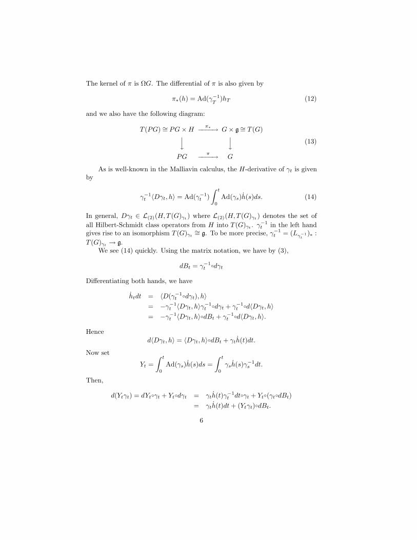
The kernel of π is ΩG. The differential of π is also given by

π∗(h) = Ad(γ−1T

)hT (12)

and we also have the following diagram:

T (PG) ∼= PG×Hπ∗−−−−→ G× g ∼= T (G)

PGπ−−−−→ G

(13)

As is well-known in the Malliavin calculus, the H-derivative of γt is givenby

γ−1t 〈Dγt, h〉 = Ad(γ−1

t )∫ t

0

Ad(γs)h(s)ds. (14)

In general, Dγt ∈ L(2)(H,T (G)γt ) where L(2)(H,T (G)γt ) denotes the set ofall Hilbert-Schmidt class operators from H into T (G)γt . γ−1

t in the left handgives rise to an isomorphism T (G)γt

∼= g. To be more precise, γ−1t = (Lγ−1

t)∗ :

T (G)γt → g.We see (14) quickly. Using the matrix notation, we have by (3),

dBt = γ−1t dγt

Differentiating both hands, we have

htdt = 〈D(γ−1t dγt), h〉

= −γ−1t 〈Dγt, h〉γ−1

t dγt + γ−1t d〈Dγt, h〉

= −γ−1t 〈Dγt, h〉dBt + γ−1

t d〈Dγt, h〉.

Henced〈Dγt, h〉 = 〈Dγt, h〉dBt + γth(t)dt.

Now set

Yt =∫ t

0

Ad(γs)h(s)ds =∫ t

0

γsh(s)γ−1s dt.

Then,

d(Ytγt) = dYtγt + Ytdγt = γth(t)γ−1t dtγt + Yt(γtdBt)

= γth(t)dt+ (Ytγt)dBt.

6

By the uniqueness of the solution, we have

〈Dγt, h〉 = Ytγt

and therefore

γ−1t 〈Dγt, h〉 = γ−1

t Ytγt = Ad(γ−1t )

∫ t

0

Ad(γs)h(s)ds

which is (14).Using the notation (8), we can rewrite (14) as

γ−1t 〈Dγt, h〉 = Ad(γ−1

t )(γ · h)(t). (15)

Since γT

= πI, we have

γ−1T

〈DγT, h〉 = Ad(γ−1

T)(γ · h)(T ) = π∗I∗(h). (16)

We have had a covariant differentiation on Pg, we can transfer it to PG,since Pg and PG are isomorphic (up to constant) to each other as Riemannianmanifolds. Let us calculate the covariant derivative.Proposition 2.2 Let Xh, Xk be right invariant vector fields associated withh, k ∈ H. Then we have

∇XhXk = Xl (17)

where

l(t) = −∫ t

0

[h(s), k(s)]ds.

Moreover we have

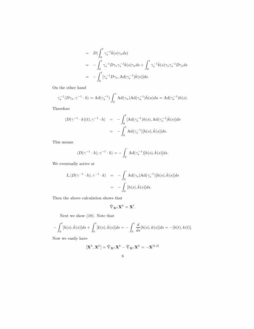
[Xh,Xk] := ∇XhXk − ∇XkXh = −X[h,k]. (18)

Here [h, k](t) := [h(t), k(t)] and [ , ] is the Lie bracket.Proof. First we note that, for γ = I(B),

I−1∗ (Xk) = γ−1 · k.

Therefore

D(γ−1 · k)(t) = D(∫ t

0

Ad(γ−1s )k(s)ds)

7

= D(∫ t

0

γ−1s k(s)γsds)

= −∫ t

0

γ−1s Dγsγ

−1s k(s)γsds +

∫ t

0

γ−1s k(s)γsγ−1

s Dγsds

= −∫ t

0

[γ−1s Dγs,Ad(γ−1

s )k(s)]ds.

On the other hand

γ−1s 〈Dγs, γ−1 · h〉 = Ad(γ−1

s )∫ s

0

Ad(γu)Ad(γ−1u )h(u)du = Ad(γ−1

s )h(s).

Therefore

〈D(γ−1 · k)(t), γ−1 · h〉 = −∫ t

0

[Ad(γ−1s )h(s),Ad(γ−1

s )k(s)]ds

= −∫ t

0

Ad(γ−1s )[h(s), k(s)]ds.

This means

〈D(γ−1 · h), γ−1 · k〉 = −∫ ·

0

Ad(γ−1s )[h(s), k(s)]ds.

We eventually arrive at

I∗〈D(γ−1 · h), γ−1 · k〉 = −∫ ·

0

Ad(γs)Ad(γ−1s )[h(s), k(s)]ds

= −∫ ·

0

[h(s), k(s)]ds.

Then the above calculation shows that

∇XhXk = Xl.

Next we show (18). Note that

−∫ t

0

[h(s), k(s)]ds +∫ t

0

[k(s), h(s)]ds = −∫ t

0

d

ds[h(s), k(s)]ds = −[h(t), k(t)].

Now we easily have

[Xh,Xk] = ∇XhXk − ∇XkXh = −X[h,k]

8

as desired.

The Lie bracket [Xk,Xh] agrees with the usual definition. For the reasonwhy the minus sign appears, see, e.g., Helgason [20, Lemma II.3.5].

Lastly we calculate the divergence. We denote the dual operator of D(with respect to PW ) by δ. For a vector field X, we define divX = −δX, X

being the 1-form associated with X, i.e.,

X(Y) = (X|Y).

For h ∈ H, we denote (Xh) by ωh. Then we have the following:Proposition 2.3 For h ∈ H,

divXh = −δωh = −∫ T

0

(h(t)|dbt)g. (19)

Here (bt) is the Brownian motion defined by (4).Proof. The vector field corresponding to Xh is γ−1 · h that is given by

(γ−1 · h)(t) =∫ t

0

Ad(γ−1s )h(s)ds.

Note that the integrand is adapted. Then it is well-known that δ(γ−1 · h) isthe stochastic integral:

δ(γ−1 · h) =∫ T

0

(Ad(γ−1s )h(s)|dBs)g.

Noticing that dbs = Ad(γs)dBs and (·|·)g is Ad(G)-invariant, we have

divXh = −δ(γ−1 · h)

= −∫ T

0

(Ad(γ−1s )h(s)|dBs)g

= −∫ T

0

(h(s)|Ad(γs)dBs)g

= −∫ T

0

(h(s)|dbs)g

which is the desired result.

9

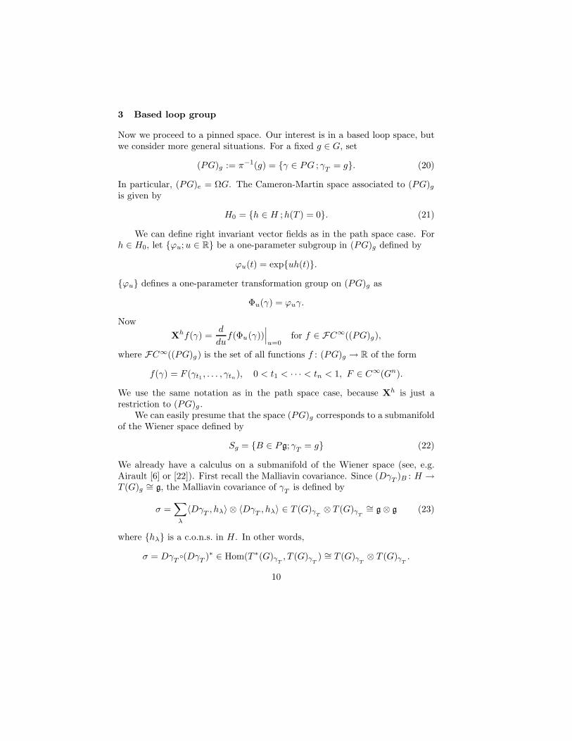
3 Based loop group

Now we proceed to a pinned space. Our interest is in a based loop space, butwe consider more general situations. For a fixed g ∈ G, set

(PG)g := π−1(g) = γ ∈ PG ; γT = g. (20)

In particular, (PG)e = ΩG. The Cameron-Martin space associated to (PG)gis given by

H0 = h ∈ H ;h(T ) = 0. (21)

We can define right invariant vector fields as in the path space case. Forh ∈ H0, let ϕu;u ∈ R be a one-parameter subgroup in (PG)g defined by

ϕu(t) = expuh(t).ϕu defines a one-parameter transformation group on (PG)g as

Φu(γ) = ϕuγ.

NowXhf(γ) =

d

duf(Φu(γ))

∣∣∣u=0

for f ∈ FC∞((PG)g),

where FC∞((PG)g) is the set of all functions f : (PG)g → R of the form

f(γ) = F (γt1 , . . . , γtn), 0 < t1 < · · · < tn < 1, F ∈ C∞(Gn).

We use the same notation as in the path space case, because Xh is just arestriction to (PG)g .

We can easily presume that the space (PG)g corresponds to a submanifoldof the Wiener space defined by

Sg = B ∈ Pg; γT

= g (22)

We already have a calculus on a submanifold of the Wiener space (see, e.g.Airault [6] or [22]). First recall the Malliavin covariance. Since (DγT )B : H →T (G)g ∼= g, the Malliavin covariance of γ

Tis defined by

σ =∑λ

〈DγT , hλ〉 ⊗ 〈DγT , hλ〉 ∈ T (G)γT⊗ T (G)γ

T

∼= g ⊗ g (23)

where hλ is a c.o.n.s. in H. In other words,

σ = DγT (DγT )∗ ∈ Hom(T ∗(G)γT, T (G)γ

T) ∼= T (G)γ

T⊗ T (G)γ

T.

10

Here the right hand side is the composite of the following mappings:

T ∗(G)γT

(DγT)∗−−−−−→ H∗ ∼= H

DγT−−−−→ T (G)γ

T

Let hλ be a c.o.n.s. of H. Now using (16), we have,

σ =∑λ

〈γ−1TDγT , hλ〉 ⊗ 〈γ−1

TDγT , hλ〉

=∑λ

Ad(γ−1T

)(γ · hλ) ⊗ Ad(γ−1T

)(γ · hλ)

=∑λ

∫ T

0

Ad(γ−1T

)Ad(γs)hλ(s)ds⊗∫ T

0

Ad(γ−1T

)Ad(γs)hλ(s)ds

=∑λ

d∑i,j=1

∫ T

0

(Ad(γ−1Tγs)hλ(s)|Xi)gds

×∫ T

0

(Ad(γ−1Tγs)hλ(s)|Xj)gdsXi ⊗Xj

=d∑

i,j=1

∑λ

∫ T

0

(hλ(s)|Ad(γ−1s γT )Xi)gds

×∫ T

0

(hλ(s)|Ad(γ−1s γ

T)Xj)gdsXi ⊗Xj

=d∑

i,j=1

∫ T

0

(Ad(γ−1s γ

T)Xi)|Ad(γ−1

s γT

)Xj)gdsXi ⊗Xj

=d∑

i,j=1

∫ T

0

(Xi|Xj)gdsXi ⊗Xj

= Td∑

i=1

Xi ⊗Xi.

Here we regard σ as an element of g ⊗ g and we used in the fifth line thatthe inner product in g is Ad(G)-invariant, i.e. Ad(γ−1

Tγs) is orthogonal. The

inverse of σ is therefore given by

σ−1 = T−1d∑

i=1

ωi ⊗ ωi ∈ g∗ ⊗ g∗ ∼= T ∗(G)γT⊗ T ∗(G)γ

T

11

where ω1, . . . , ωd is the dual basis of X1, . . . ,Xd. Then the tangent spaceof Sg is given by

T (Sg) = h ∈ H; 〈DγT , h〉 = 0. (24)

By this definition and (16), it is easy to see that h ∈ T (Sg) if and only if(γ · h)(T ) = I∗(h)(T ) = 0. Therefore I∗ : T (S)B → H0 is again an isomor-phism preserving inner products. Sg is isomorphic to (PG)g as a Riemannianmanifold. We can identify Sg and (PG)g with one another. On the submani-fold Sg, we can define Γ(T (Sg)) to be the set of smooth sections of T (Sg) (see,e.g. [22]) and therefore, by using I, we can define the set of smooth sectionson T ((PG)g) and denote it by Γ(T ((PG)g)).

It is easy to see that

H⊥0 = Xψ;X ∈ g (25)

where ψt = t/√T . Let p : H → H0, q : H → H⊥

0 be orthogonal projections.Then they can be written as

ph = h− h(T )√Tψ (26)

qh = h(T )√Tψ. (27)

The normal bundle is defined as the image of q and denoted by N((PG)g).Since g X → Xψ ∈ H⊥

0 gives an isomorphism, we identify H⊥0 with g.

Therefore N((PG)g) ∼= (PG)g × gNow the covariant differentiation on (PG)g is defined by

∇XY := p∇XY, X,Y ∈ Γ(T ((PG)g)).

The second fundamental form A is given by

A(X,Y) = q∇XY = ∇XY −∇XY.

Proposition 3.1 For h, k ∈ H0,

A(Xh,Xk) = − 1√T

∫ T

0

[h(s), k(s)]ds (28)

Proof. By Proposition 2.2, ∇XhXk = Xl where

l(t) = −∫ t

0

[h(s), k(s)]ds.

12

Hence

A(Xh,Xk) = ql = − 1√T

∫ T

0

[h(s), k(s)]ds,

which is the desired result.

By using the second fundamental form, we can express the Riemanniancurvature as follows (see, e.g. [31, Proposition 26], [22, Theorem 3.5]):

R(X,Y,Z,W) = −(A(X,Z)|A(Y,W))g + (A(Y,Z)|A(X,W))g .(29)

Let us introduce the area measure m on (PG)g as follows (for the areameasure, see [7]):

m = δg(γT )√

detσ.

Since det σ = T d, we have

m = T d/2 pT (e, g)E[ · |γT = g]

Here pT (e, g) denotes the probability density function of the law of γT . Thusm differs from the pinned measure E[ · |γ

T= g] up to constant. Let ∇∗ be

the dual operator of ∇ with respect to m. Then ∇∗ can be written as

∇∗ = δ − 12i((Dγ

Tlog det σ))

(see, [23, §2]) where i(·) denotes the interior product. Therefore we have ∇∗ = δbecause det σ is constant. For a vector field X, we define divX = −∇∗X, X

being the 1-form associated with X, i.e.,

X(Y) = (X|Y).

In the sequel, we denote (Xh) by ωh. By Proposition 2.3, we easily haveProposition 3.2 For h ∈ H0,

divXh = −∇∗ωh = −∫ T

0

(h(t)|dbt)g. (30)

Here (bt) is the Brownian motion defined by (4).Let us proceed to define the Ricci curvature. By using the second funda-

mental form, we can write the Ricci curvature as follows (see, e.g. [15], [23]):

Ric(·, ·) = −∑λ

(A(·,Xhλ )|A(·,Xhλ )) + (A(·, ·)|qδq) (31)

where hλ is a c.o.n.s. of H0. First we calculate qδq.

13

Lemma 3.3 It holds that

qδq =bT√T. (32)

Proof. We first note that the projection operator to T (Sg) which we denoteby Q, can be written as follows:

Qh = I−1∗ (q(I∗h))

= I−1∗ (q(γ · h))

= I−1∗

( 1√T

(γ · h)(T )ψ)

=1T

∫ ·0

Ad(γ−1t )(γ · h)(T )dt.

For a c.o.n.s. hλ of H, we can write

δQ = δ∑λ

(hλ|Q(·))H ⊗ hλ =∑λ

δ(hλ|Q(·))Hhλ.

Here for h ∈ H,

(hλ|Q(h)) =1T

∫ T

0

(hλ(t)

∣∣∣Ad(γ−1t )

∫ T

0

Ad(γs)h(s)ds)

gdt

=1T

∫ T

0

∫ T

0

(Ad(γ−1s γt)hλ(t)|h(s))gds dt.

Hence

(hλ|Q(·))H =1T

∫ ·0

ds

∫ T

0

Ad(γ−1s γt)hλ(t)dt

=1T

∫ ·0

ds

∫ s

0

Ad(γ−1s γt)hλ(t)dt

+1T

∫ ·0

ds

∫ T

s

Ad(γ−1s γt)hλ(t)dt.

Here we identify H∗ with H. Since the integrand of the first term is adapted,we have

δ( 1T

∫ ·0

ds

∫ s

0

Ad(γ−1s γt)hλdt

)=

1T

∫ T

0

(∫ s

0

Ad(γ−1s γt)hλ(t)dt

∣∣∣dBs

)g

14

=1T

∫ T

0

(∫ s

0

Ad(γt)hλ(t)dt∣∣∣Ad(γs)dBs

)g

=1T

∫ T

0

((γ · hλ)(s)|dbs)g.

We calculate the second term. To do this, we use an approximation argument.Let = 0 = s0 < s1 < · · · < sN = T be a partition of [0, T ] and we set|| = maxsk − sk−1; k = 1, . . . , N. Then

1T

∫ ·0

ds

∫ T

s

Ad(γ−1s γt)hλ(t)dt

= lim||→0

1T

N∑k=1

∫ T

sk

Ad(γ−1skγt)hλ(t)dt

∫ ·0

1[sk−1,sk](s)ds.

Here, the convergence in the right hand side is the strong convergence inLp(Pg, PW ) for all p ≥ 1. On the other hand, since (γt) is a left Brown-ian motion, it holds that, for t ≥ s

γ−1s γt = γt−s(θsB)

where θs is a shift operator: (θsB)u = Bs+u −Bs. We can see that for t ≥ s

〈DAd(γ−1s γt), h〉 = 0

if supph ⊆ [0, s]. By virtue of this fact, we have

δ 1T

N∑k=1

∫ T

sk

Ad(γ−1skγt)hλ(t)dt

∫ ·0

1[sk−1,sk](s)ds

= − 1T

N∑k=1

d∑i=1

(D

∫ T

sk

(Ad(γ−1skγt)hλ(t)|Xi)gdt

∣∣∣ ∫ ·0

Xi1[sk−1,sk](s)ds)H

+1T

N∑k=1

d∑i=1

∫ T

sk

(Ad(γ−1skγt)hλ(t)|Xi)gdt δ

∫ ·0

Xi1[sk−1,sk](s)ds

=1T

N∑k=1

(∫ T

sk

Ad(γ−1skγt)hλ(t)dt

∣∣∣Bsk −Bsk−1

)g

=1T

N∑k=1

N−1∑l=k

(∫ sl+1

sl

Ad(γt)hλ(t)dt∣∣∣Ad(γsk )(Bsk −Bsk−1)

)g

15

=1T

N−1∑l=1

(∫ sl+1

sl

Ad(γt)hλ(t)dt∣∣∣ l∑k=1

Ad(γsk)(Bsk −Bsk−1))

g.

We notice that

lim||→0

∑k: sk≤t

Ad(γsk)(Bsk −Bsk−1) = 2∫ t

0

Ad(γs)dBs −∫ t

0

Ad(γs)dBs

= bt.

Here we used Proposition 2.1. Accordingly, by using the Ito formula, we have

lim||→0

δ 1T

N∑k=1

∫ T

sk

Ad(γ−1skγt)hλ(t)dt

∫ ·0

1[sk−1,sk](s)ds

=1T

∫ T

0

(Ad(γt)hλ(t)|bt)gdt

=1T

(∫ T

0

Ad(γt)hλ(t)dt|bT )g − 1T

∫ T

0

(∫ t

0

Ad(γs)hλ(s)ds|dbt)g

=1T

((γ · hλ)(T )|bT )g − 1T

∫ T

0

((γ · hλ)(t)|dbt)g.

Thus we have

δ(hλ|Q(·))H =1T

∫ T

0

((γ · hλ)(s)|dbs)g +1T

((γ · hλ)(T )|bT )g

− 1T

∫ T

0

((γ · hλ)(t)|dbt)g

=1T

((γ · hλ)(T )|bT )g.

By summing up over λ we have

∑λ

δ(hλ|q(·))Hhλ =1T

∑λ

((γ · hλ)(T )|bT )ghλ.

Now we have

qδq = I∗(QδQ)

=1T

∑λ

((γ · hλ)(T )|bT )gI∗(qhλ)

16

=1T

∑λ

((γ · hλ)(T )|bT )g1√T

(γ · hλ)(T )

=1

T 3/2

∑λ

d∑i=1

(∫ T

0

Ad(γs)hλ(s)ds|bT )g(∫ T

0

Ad(γs)hλ(s)ds|Xi)g Xi

=1

T 3/2

d∑i=1

∑λ

∫ T

0

(hλ(s)|Ad(γ−1s )bT )gds

∫ T

0

(hλ(s)|Ad(γ−1s )Xi)gdsXi

=1

T 3/2

d∑i=1

∫ T

0

(Ad(γ−1s )bT |Ad(γ−1

s )Xi)gdsXi

=1

T 3/2

d∑i=1

T (bT |Xi)g Xi

=1√TbT

which completes the proof.

Now we can calculate the Ricci curvature as follows:Proposition 3.4 The Ricci curvature is written as

Ric(Xh,Xk) =1T

∫ T

0

K(h(s), k(s))ds +1√T

(bT |A(Xh,Xk))g (33)

− 1T 2

∫ T

0

∫ T

0

K(h(s), k(t))dsdt

where K is the Killing form defined by K(X,Y ) = tr(adXadY ).Proof. It is enough to calculate

∑λ(A(·,Xhλ )|A(·,Xhλ )). Since (·, ·)g is Ad(G)

invariant, adX is skew-symmetric for X ∈ g. Hence, for X,Y ∈ g,∑i

(adX(Xi)|adY (Xi))g = −∑i

(Xi|adXadY (Xi))g

= −tr(adXadY )= −K(X,Y ).

Using this and noting that hλ ∪ Xiψ forms a c.o.n.s. of H, we have

∑λ

(A(Xh,Xhλ )|A(Xk ,Xhλ))g

17

=1T

∑λ

(∫ T

0

[h(s), hλ(s)]ds∣∣∣ ∫ T

0

[k(t), hλ(t)]dt)

g

=1T

∑λ

d∑i=1

∫ T

0

(adh(s)(Xi)|hλ(s))gds∫ T

0

(adk(t)(Xi)|hλ(s))gdt

=1T

d∑i=1

∫ T

0

(adh(s)(Xi)|adk(s)(Xi))gds

− 1T

d∑i,j=1

∫ T

0

(adh(s)(Xi)|Xjψ(s))gds∫ T

0

(adk(t)(Xi)|Xjψ(t))gdt

= − 1T

∫ T

0

K(h(s), k(s))ds +1T 2

d∑i=1

∫ T

0

∫ T

0

(adh(s)(Xi)|adk(t)(Xi))gds dt

= − 1T

∫ T

0

K(h(s), k(s))ds +1T 2

∫ T

0

∫ T

0

K(h(s), k(t))dsdt.

This completes the proof.

We set ∆ = −∇∗∇. Here ∆ acts on scalar-valued functions. Recall thatthe Bakry-Emery Γ2 is defined by

Γ2(f, g) :=12∆(∇f |∇g)− (∇∆f |∇g)− (∇f |∇∆g).

Then the following formula for Γ2 can be found in Getzler [15] and Airault [6](see also [23]).

Γ2(f, g) = (∇2f |∇2g) + (∇f |∇g) + Ric((∇f), (∇g)). (34)

We give an estimate for the norm of A. Let M be a constant satisfying

|[X,Y ]|g ≤M |X|g|Y |g. (35)

Then we have

‖A‖ := sup|h|H , |k|H≤1

|A(Xh,Xk)|g ≤ M√T . (36)

To see this,

|A(Xh,Xk)|g ≤ 1√T

∫ T

0

|[h(t), k(t)]|gdt

18

≤ M√T

∫ T

0

|h(t)|g|k(t)|gdt

≤ M√T

supt∈[0,T ]

|h(t)|g∫ T

0

|k(t)|gdt

≤ M√T

∫ T

0

|h(t)|gdt∫ T

0

|k(t)|gdt

≤ M√TT

∫ T

0

|h(t)|2gdt1/2∫ T

0

|k(t)|2gdt1/2

= M√T |h|H |k|H .

This shows (36).The lower bound of the Ricci curvature is essential in the later argument.

Since G is compact, the Killing form K is negative definite. Therefore, we haveto estimate the first term in (33). We can see

|K(X,Y )| = |∑i

(adX(Xi)|adY (Xi))g| ≤∑i

M2d|X|g|Y |g.

Hence ∣∣∣ 1T

∫ T

0

K(h(s), k(s))ds∣∣∣ ≤ M2d sup

t∈[0,T ]

|h(t)|g supt∈[0,T ]

|k(t)|g (37)

≤ M2dT |h|H |k|H .

4 Spectral gap

The spectral gap for the operator ∇∗∇ is a fundamental problem. In thissection we give a sufficient condition for the spectral gap. But unfortunately,the author does not know any example satisfying this sufficient condition.First we change the reference measure. Set µ = e−2Udm. Here U is a smoothfunction in the sense of Malliavin. We consider the following Dirichlet form inL2((PG)g , µ):

E(f, h) =∫

(PG)g

(∇f |∇h)dµ. (38)

We denote the norm in Lp((PG)g , µ) by ‖ · ‖p. We assume the followinglogarithmic Sobolev inequality for E: there exists a constant λ > 0 and anon-negative potential function V such that∫

(PG)g

f2 log(f2/‖f‖22)dµ ≤ λE(f, f) +

∫(PG)g

V f2dµ. (39)

19

The generator associated with E can be calculated as follows: for η ∈Γ(T ∗((PG)g))∫

(PG)g

(∇f |η)e−2Udm =∫

(PG)g

f(∇∗ηe−2U − (∇e−2U |η)dm

=∫

(PG)g

f(∇∗η + 2(∇U |η))e−2Udm.

Hence the dual operator of ∇ with respect to µ is ∇∗ + 2(∇U |·). Thereforethe generator AU can be written as

AU = −(∇∗ + 2(∇U |·))∇ = −∇∗∇− 2(∇U |∇·) = ∆ − 2(∇U |∇·).Then, by (33), the Bakry-Emery Γ2 in this case is given by

Γ2(f, g) =12AU (∇f |∇g) − (∇AUf |∇g) − (∇f |∇AUg)

= (∇2f |∇2g) + (∇f |∇g) + Ric((∇f), (∇g))+ 2∇2U((∇f), (∇g)).

Clearly AU is non-negative definite and AU1 = 0. The following lemma iseasy:Lemma 4.1 If there exists a constant c > 0 such that∫

(PG)g

Γ2(f, f)dµ ≥ c

∫(PG)g

(∇f |∇f)dµ. (40)

Then AU has a spectral gap. To be precise, denoting the set of spectrum of−AU by σ(−AU ), it holds that

infσ(−AU ) \ 0 ≥ c. (41)

Proof. Note that ∫(PG)g

Γ2(f, f)dµ =∫

(PG)g

(AUf)2dµ

and ∫(PG)g

(∇f |∇f)dµ = −∫

(PG)g

(AUf)fdµ.

Then the assertion is an easy consequence of the spectral theorem.

20

Remark 4.1 The above proof shows that (40) and (41) are equivalent to oneanother.

Now we have the following main theorem.Theorem 4.2 Assume that there exists a constant c > 0 such that for anyh ∈ H0,(

1 − dM2T +1λ− 1λ‖eλM |bT |‖1 − V

λ− c

)|Xh|2 + 2∇2U(Xh,Xh) ≥ 0.

(42)

Then AU has a spectral gap.Proof. We check the assumption of Lemma 4.1. By Proposition 3.4, (36) and(37), we easily have

Ric(Xh,Xh) ≥ −(|bT |/√T )‖A‖|h|2H − dM2T |h|2H

≥ −M |bT ||h|2H − dM2T |h|2H .

Hence,

Γ2(f, f)= (∇2f |∇2f) + (∇f |∇f) + Ric((∇f), (∇f)) + 2∇2U((∇f), (∇f))≥ |∇2f |2 + |∇f |2 −M |bT ||∇f |2 − dM2T |∇f |2 + 2∇2U((∇f) , (∇f)).

Now we notice that from (39) we have∫(PG)g

|∇f |2 log(|∇f |2/‖∇f‖22)dµ ≤ λ

∫(PG)g

|∇2f |2dµ +∫

(PG)g

V |∇f |2dµ.(43)

Further recall the Young inequality st ≤ s log s − s + et (s > 0, t ∈ R). Com-bining these inequalities, we have∫

(PG)g

Γ2(f, f)dµ

≥∫

(PG)g

|∇2f |2dµ + (1 − dM2T )∫

(PG)g

|∇f |2dµ

−∫

(PG)g

M |bT ||∇f |2dµ +∫

(PG)g

2∇2U((∇f), (∇f))dµ

≥∫

(PG)g

|∇2f |2dµ + (1 − dM2T )∫

(PG)g

|∇f |2dµ

21

− 1λ

∫(PG)g

|∇f |2(λM |bT |)dµ +∫

(PG)g

2∇2U((∇f), (∇f))dµ

≥∫

(PG)g

|∇2f |2dµ + (1 − dM2T )∫

(PG)g

|∇f |2dµ

− 1λ

∫(PG)g

|∇f |2 log |∇f |2dµ +1λ

∫(PG)g

|∇f |2dµ

− 1λ

∫(PG)g

eλM |bT |dµ + 2∫

(PG)g

∇2U((∇f), (∇f))dµ

≥∫

(PG)g

|∇2f |2dµ + (1 − dM2T )∫

(PG)g

|∇f |2dµ−∫

(PG)g

|∇2f |2dµ

− 1λ

∫(PG)g

V |∇f |2dµ− 1λ‖∇f‖2

2 log ‖∇f‖22 +

1λ

∫(PG)g

|∇f |2dµ

− 1λ

∫(PG)g

eλM |bT |dµ + 2∫

(PG)g

∇2U((∇f), (∇f))dµ

≥∫

(PG)g

(1 − dM2T +

1λ− V

λ

)|∇f |2dµ− ‖∇f‖2

2 log ‖∇f‖22

− 1λ

∫(PG)g

eλM |bT |dµ + 2∫

(PG)g

∇2U((∇f), (∇f))dµ.

Replacing f by f/‖∇f‖2 (we may assume that ‖∇f‖2 = 0), we have∫(PG)g

Γ2(f, f)dµ ≥∫

(PG)g

(1 − dM2T +

1λ− 1λ‖eλM |bT |‖1 − V

λ

)|∇f |2

+2∇2U((∇f) , (∇f))dµ

≥ c

∫(PG)g

|∇f |2dµ.

This completes the proof.

References

[1] S. Aida, Certain gradient flows and submanifolds in Wiener spaces, J.Funct. Anal., 112 (1993), 346–372.

[2] S. Aida, On the Ornstein-Uhlenbeck Operators on Wiener-RiemannianManifolds, J. Funct. Anal., 116 (1993), 83–110.

22

[3] S. Aida, Sobolev Spaces over Loop Groups, J. Funct. Anal., 127 (1995),155–172.

[4] S. Aida, Essential selfadjointness of Ornstein-Uhlenbeck operators on loopgroups, preprint

[5] S. Aida and I. Shigekawa, Logarithmic Sobolev inequalities and spectralgaps: perturbation theory, J. Funct. Anal., 126 (1994), 448–475.

[6] H. Airault, Differential calculus on finite codimensional submanifolds ofthe Wiener space—The divergence operator, J. Funct. Anal., 100 (1991),291–316.

[7] H. Airault and P. Malliavin, Integration geometrique sur l’espace deWiener, Bull. Sci. Math., 112 (1988), 3–52.

[8] H. Airault and P. Malliavin, Integration on loop groups. II. Heat equationfor the Wiener measure, J. Funct. Anal., 104 (1992), 71–109.

[9] H. Airault and J. Van Biesen, Geometrie riemannienne en codimensionfinie sur l’espace de Wiener, C. R. Acad. Sci. Paris Serie I, 311 (1990),125–130.

[10] H. Airault and J. Van Biesen, Le processus d’Ornstein-Uhlenbeck sur unesous-variete de l’espace de Wiener, Bull. Sci. Math., 115 (1991), 185–210.

[11] S. Albeverio and R. Høegh-Krohn, The energy representation of SobolevLie groups, Compositio Math., 36 (1978), 37–52.

[12] B. K. Driver, A Cameron-Martin type quasi-invariance theorem for Brow-nian motion on a compact Riemannian manifold, J. Funct. Anal., 110(1992), 272–376.

[13] S. Fang, Inegalite du type de Poincare sur un espace de chemins, preprint.

[14] D. S. Freed, The geometry of loop groups, J. Diff. Geom., 28 (1988),223–276.

[15] E. Getzler, Dirichlet forms on loop space, Bull. Sci. Math., 113 (1989),151–174.

[16] L. Gross, Logarithmic Sobolev inequalities, Amer. J. Math., 97 (1975),1061–1083.

[17] L. Gross, Logarithmic Sobolev inequalities on loop groups, J. Funct.Anal., 102 (1991), 268–313.

[18] L. Gross, Logarithmic Sobolev inequality over some infinite dimensionalmanifolds, Proceedings of the conference on probability models in mathe-matical physics, ed. by G. J. Morrow and W.-S. Yang, pp. 98–107, WorldScientific, Singapore, 1991.

23

[19] L. Gross, Uniqueness of ground states for Schrodinger operators over loopgroups, J. Funct. Anal., 112 (1993), 373–441.

[20] S. Helgason, “Differential geometry, Lie groups, and symmetric spaces,”Academic Press, New York, 1978.

[21] N. Ikeda and S. Watanabe, “Stochastic differential equations and diffusionprocesses,” North Holland/Kodansha, Amsterdam/Tokyo, 1981.

[22] T. Kazumi and I. Shigekawa, Differential calculus on a submanifold ofan abstract Wiener space, I. Covariant derivative, in “Stochastic analysison infinite dimensional spaces,” ed. by H. Kunita and H.-H. Kuo, pp.117–140, Longman, Harlow, 1994.

[23] T. Kazumi and I. Shigekawa, Differential calculus on a submanifold of anabstract Wiener space, II. Weitzenbock formula, in “Dirichlet forms andstochastic processes,” Proceedings of the International Conference held inBeijing, China, October 25-31, 1993, ed. by Z. M. Ma, M. Rockner andJ. A. Yan, pp. 235–251, Walter de Gruyter, Berlin-New York, 1995.

[24] M.-P. Malliavin and P. Malliavin, Integration on loop groups. I. QuasiInvariant measures, J. Funct. Anal., 93 (1990), 207–237.

[25] M.-P. Malliavin and P. Malliavin, Integration on loop groups. III. Asymp-totic Peter-Weyl orthogonality, J. Funct. Anal., 108 (1992), 13–46.

[26] A. Pressley and G. Segal, “Loop groups,” Oxford University Press, NewYork, 1986.

[27] I. Shigekawa, Transformations of the Brownian motions on the Lie group,Proceedings of the Taniguchi International Symposium on StochasticAnalysis, Katata and Kyoto, 1982, pp. 409–422, (1984).

[28] I. Shigekawa, De Rham-Hodge-Kodaira’s decomposition on an abstractWiener space, J. Math. Kyoto Univ., 26 (1986), 191–202.

[29] I. Shigekawa, A quasi-homeomorphism on the Wiener space, Proceedingsof Symposia in Pure Mathematics, vol. 57, Stochastic Analysis, ed. byM. Cranston, M. A. Pinsky, pp. 473–486, American Mathematical Society,Providence, 1995.

[30] I. Shigekawa and S. Taniguchi, A Kahler metric on a based loop groupand a covariant differentiation, preprint

[31] J. Van Biesen, The divergence on submanifolds of the Wiener space, J.Funct. Anal., 113 (1993), 426–461.

24