1

Differential dissipativity theoryfor dominance analysis

Fulvio Forni, Rodolphe Sepulchre

Abstract—High-dimensional systems that have a low-dimensional dominant behavior allow for model reduction andsimplified analysis. We use differential analysis to formalizethis important concept in a nonlinear setting. We show thatdominance can be studied through linear dissipation inequalitiesand an interconnection theory that closely mimics the classicalanalysis of stability by means of dissipativity theory. In thisapproach, stability is seen as the limiting situation where the dom-inant behavior is 0-dimensional. The generalization opens noveltractable avenues to study multistability through 1-dominanceand limit cycle oscillations through 2-dominance.

I. INTRODUCTION

The analysis of a system is considerably simplified whenit is low-dimensional. Linear system analysis frequently ex-ploits the property that a few dominant poles capture themain properties of a possibly high-dimensional system. Low-dimensional models are even more critical in nonlinear systemanalysis. Multistability or limit cycle analysis is difficultbeyond the phase plane analysis of two-dimensional systems.

In this paper we seek to formalize the property that anonlinear system has low-dimensional dominant behavior. Ourapproach is differential: we characterize the property for linearsystems and then study the nonlinear system differentially, thatis, along the linearized flow in the tangent bundle. The seminalexample of differential analysis in control theory is contractionanalysis [26], [34], [15], [37], [43], which we interpret asa differential analysis of exponential stability. The propertyis the contraction of a ball, characterized via a Lyapunovdissipation inequality. A nonlinear system is contractive whenthis dissipation inequality holds infinitesimally along any of itstrajectories. In the present paper, the corresponding propertyis 0-dominance: it ensures that the dominant behavior of thenonlinear system is 0-dimensional. A more recent example ofdifferential analysis is differential positivity [12], the differen-tial analysis of positivity. The linear property is the contractionof a cone, also characterized by a dissipation inequality. Anonlinear system is differentially positive when this dissipationinequality holds infinitesimally along any of its trajectories. Inthe context of the present paper, the corresponding propertyis 1-dominance: it guarantees that the dominant behavior ofthe nonlinear system is 1-dimensional. More generally, westudy the property of p-dominance differentially. The property

F. Forni and R. Sepulchre are with the University of Cambridge,Department of Engineering, Trumpington Street, Cambridge CB2 1PZf.forni@eng.cam.ac.uk|r.sepulchre@eng.cam.ac.uk. Theresearch leading to these results has received funding from the EuropeanResearch Council under the Advanced ERC Grant Agreement Switchletn.670645.

is characterized via a dissipation inequality, which is thenrequired to hold infinitesimally along the trajectories of thenonlinear system. We prove a general theorem that formalizesthat the dominant behavior of a p-dominant system is p-dimensional.

Differential analysis is general in that it allows to extenda linear system property to an arbitrary flow defined on adifferentiable manifold. An important restriction in this paperis that we only consider dissipation properties characterized bylinear matrix inequalities. Furthermore, we impose the lineardissipation inequality to be uniform on the tangent bundle.In geometric terms, this endows the differentiable manifoldwith a flat non-degenerate metric structure, characterized by aconstant quadratic form.

The linear-quadratic restriction allows for a fruitful bridgewith the linear-quadratic theory of dissipativity. Many of theavailable computational tools of dissipativity theory becomeavailable for the analysis of p-dominance. The analysis ofp-dominance is reformulated as the search of a quadraticdifferential storage that decreases along the solutions of thelinearized dynamics. The classical interconnections theoremsof (linear-quadratic) dissipativity theory are reformulated astools that facilitate that construction. The only substantialdifference with the classical theory is that the quadratic formthat characterizes the storage is no longer required to be aLyapunov function, i.e. positive definite. Instead, it is requiredto have a fixed inertia, that is, p negative eigenvalues and n−ppositive eigenvalues. Stability corresponds to p = 0, whereasp-dominance allows for any integer 0 ≤ p ≤ n.

The paper is organized as follows. Section II characterizesp-dominance and p-dissipativity for linear time-invariant mod-els. Section III defines p-dominance for nonlinear systems withtwo main results that characterize their asymptotic behavior.The connection with related results in the literature is dis-cussed in Section IV and dominance analysis via the solutionof LMIs is illustrated in Section IV. Differential p-dissipativityis addressed in Section VI, where we primarily illustratethe role of differential passivity and differential small-gaintheorems in the design and analysis of multistable systems(p = 1) and limit cycle oscillations (p = 2). The proofs of themain theorems are provided in appendix.

II. DOMINANT LTI SYSTEMS

Definition 1: A linear system x = Ax is p-dominant withrate λ ≥ 0 if and only if there exist a symmetric matrix Pwith inertia (p, 0, n− p) such that

ATP + PA ≤ −2λP − εI . (1)

arX

iv:1

710.

0172

1v2

[cs

.SY

] 5

Oct

201

7

2

for some ε ≥ 0. The property is strict if ε > 0. yIn terms of the quadratic form V (x) = xTPx, the (strict)

dissipation inequality (1) reads

V (x) = xT (ATP + PA)x

≤ −2λV (x)− ε | x |2

For ε > 0 this implies that the two cones

K− = x ∈ Rn | V (x) ≤ 0, K+ = x ∈ Rn | V (x) ≥ 0are strictly contracting either in forward or in backward time:

∀t > 0 : e−AtK+ ⊂ K+, eAtK− ⊂ K−

Equivalent characterizations of p-dominance are provided inthe following proposition, whose proof is in the preliminaryversion of this paper [13].

Proposition 1: For ε > 0, the Linear Matrix Inequality (1)is equivalent to any of the following conditions:

1) The matrix A + λI has p eigenvalues with strictlypositive real part and n − p eigenvalues with strictlynegative real part.

2) there exists an invariant subspace splitting Rn = H⊕Vsuch that AH ⊂ H and AV ⊂ V . The dimension of V isn− p and the dimension of H is p. Furthermore, thereexist constants 0 < C ≤ 1 ≤ C and λ < λ < λ suchthat

∀x ∈ H : | eAtx |≥ C e−λt | x |, t ≥ 0

∀x ∈ V : | eAtx |≤ C e−λt | x |, t ≥ 0.

yThe property of p-dominance ensures a splitting between

n − p transient modes and p dominant modes. Only thep dominant modes dictate the asymptotic behavior. Becauseλ ≥ 0 and V ⊂ K+, the quadratic form V (x) is a Lyapunovfunction for the transient behavior, that is, for the restrictionof the flow in V .

For p = 0, p-dominance is the classical property of expo-nential stability: all modes are transient and the asymptoticbehavior is 0-dimensional.

The matrix inequality (1) is equivalent to the conic con-straint [

xx

]T[0 PP 2λP + εI

] [xx

]≤ 0. (2)

Dissipativity theory extends p-dominance to open systemsby augmenting the internal dissipation inequality with anexternal supply. The external property of p-dissipativity iscaptured by a conic constraint between the state of the systemx, its derivative x, and the external variables y and u of theform[

xx

]T[0 PP 2λP + εI

][xx

]≤[yu

]T[Q LLT R

][yu

](3)

where P is a matrix with inertia (p, 0, n− p), λ ≥ 0, L,Q,Rare matrices of suitable dimension, and ε ≥ 0. The propertyis strict if ε > 0. We call supply rate s(y, u) := yTQy +yTLu+ uTLT y + uTRu the right-hand side of (3). An opendynamical system is p-dissipative with rate λ if its dynamicsx = Ax+Bu, y = Cx+Du satisfy (3) for all x and u.

p-dissipativity has a simple characterization in terms oflinear matrix inequalities.

Proposition 2: A linear system x = Ax+Bu, y = Cx+Duis p-dissipative with rate λ ≥ 0 if and only if there exists asymmetric matrix P with inertia (p, 0, n− p) such that[

ATP+PA+2λP−CTQC+εI PB−CTL−CTQDBTP−LTC−DTQC −DTQD−LTD−DTL−R

]≤ 0 . (4)

yProof: [⇒] Just replace x = Ax+Bu and y = Cx+Du

in (3) and rearrange. [⇐] Multiply (4) by [xT uT ] on the left,and by [xT uT ]T on the right. Then we get xTPx+ xTPx+2λxTPx < s(y, u) as desired.

An interconnection theorem can be easily derived. A proofis provided in the preliminary version of this paper [13].

Proposition 3: Let Σ1 and Σ2 p1-dissipative and p2-dissipative systems respectively, with uniform rate λ and withsupply rate

si(yi, ui) =

[yu

]T[Qi LiLTi Ri

] [yu

](5)

for i ∈ 1, 2. The closed-loop system given by negativefeedback interconnection

u1 = −y2 + v1 u2 = y1 + v2 (6)

is (p1 + p2)-dissipative with rate λ from v = (v1, v2) to y =(y1, y2) with supply rate

s(y, v) =

[yv

]T Q1 +R2 −L1 + LT2 L1 R2

−LT1 + L2 Q2 +R1 −R1 L2

LT1 −R1 R1 0R2 LT

2 0 R2

[yv

].

(7)The closed loop is (p1 + p2)-dominant with rate λ if[

Q1 +R2 −L1 + LT2−LT1 + L2 Q2 +R1

]≤ 0 . (8)

yMimicking classical dissipativity theory, there are two im-

portant particular cases of supply rates : the passivity supply

s(y, u) =

[yu

]T[0 II 0

] [yu

]. (9)

and the gain supply:

s(y, u) =

[yu

]T[ −I 00 γ2I

] [yu

]. (10)

Hence, Proposition 3 provides an analog of the small-gaintheorems and passivity theorems for p-dominance of a lineartime-invariant system.

III. DIFFERENTIAL ANALYSIS OFDOMINANT NONLINEAR SYSTEMS

For a nonlinear system

x = f(x) x ∈ X (11)

we define dominance differentially, that is, through the lineardissipation inequality[

˙δxδx

]T[0 PP 2λP + εI

] [˙δxδx

]≤ 0 (12)

3

for every δx ∈ TxX , where P is a matrix with inertia (p, 0, n−p) and ε ≥ 0.

In what follows we assume that X is a smooth Riemannianmanifold of dimension n. Given any δx ∈ TxX , |δx| denotesthe Riemanian metric on X represented by

√δxTδx in local

coordinates. ψt(x) denotes the flow of (11) at time t passingthrough x ∈ X at time 0. ∂ψt(x) denotes the differential ofψt(x) with respect to x. Note that (ψt(x), ∂ψt(x)δx) is a flowin the tangent bundle. It is the solution of the prolonged system[6]

x = f(x)˙δx = ∂f(x)δx

(x, δx) ∈ TX (13)

at time t passing through (x, δx) ∈ TX at time 0. In localcoordinates ∂f(x) denotes the differential of f at x and P isthe local representation of a metric tensor P with fixed inertia.

Following the approach of Section II, we define the propertyof dominance for nonlinear systems as follows.

Definition 2: A nonlinear system x = f(x) is p-dominantwith rate λ ≥ 0 if and only if there exist a symmetric matrixP with inertia (p, 0, n − p) such that (12) is satisfied by thesolutions of the prolonged system (13) for some ε ≥ 0. Theproperty is strict if ε > 0. y

In terms of the quadratic function V (δx) := δxTPδx, thedifferential dissipation inequality (12) reads

V (δx) = δxT(∂f(x)TP + P∂f(x)

)δx

≤ −2λV (δx)− ε | δx |2 (14)

As a consequence, for ε > 0, the two cone fields

K+(x) := δx ∈ TxX |V (δx) ≥ 0,K−(x) := δx ∈ TxX |V (δx) ≤ 0

are strictly contracting either in forward time or in backwardtime, respectively:

∂ψ−t(x)K+(x) ⊂ K+(ψ−t(x)) ∀t > 0

∂ψt(x)K−(x) ⊂ K−(ψt(x)) ∀t > 0

The following result provides the differential analog ofProposition 1.

Theorem 1: Let A ⊆ X be a compact invariant set and let(11) be a strictly p-dominant system with rate λ ≥ 0 and tensorP . Then, for each x ∈ A, there exists an invariant splittingTxX = Hx ⊕ Vx

∂ψt(x)Hx ⊆ Hψt(x) ∀t ∈ R ,∂ψt(x)Vx ⊆ Vψt(x) ∀t ∈ R .

(15)

Hx and Vx are distributions of dimension p and n − p,respectively. Furthermore, there exist constants C ≤ 1 ≤ Cand λ < λ < λ such that

|∂ψt(x)δx| ≥ Ce−λt|δx| ∀x ∈ A,∀δx ∈ Hx (16a)

|∂ψt(x)δx| ≤ Ce−λt|δx| ∀x ∈ A,∀δx ∈ Vx . (16b)

yThe interpretation of the theorem is that the linearized flow

∂ψt(·) admits an invariant splitting between n − p transientmodes and p dominant modes. The p dominant modes dictatethe long-term behavior of the flow. The quadratic form V (δx)

is a differential Lyapunov function in the invariant distributionV ⊂ TX .

For X = Rn the characterization of the asymptotic behaviorof dominant systems can be further refined. This is because,by integration, the differential dissipation inequality (14) leadsto the incremental inequality

V (x−y) = (x−y)TP (f(x)−f(y))+(f(x)−f(y))TP (x−y)

= 2(x− y)(∫ 1

0P∂f(sx+ (1−s)y)ds

)(x− y)

≤ −ε(x− y)T(∫ 1

0−2λP + εI ds

)(x− y)

≤ −2λV (x− y)− ε | x− y |2 .(17)

The following result is based on the incremental dissipationinequality (17). We denote by Ω(x) the ω-limit set of x, thatis, the set of all ω-limit points of x.

Theorem 2: For X = Rn, let (11) be a strictly p-dominantsystem with rate λ ≥ 0. Then, the flow on any compact ω-limit set is topologically equivalent to a flow on a compactinvariant set of a Lipschitz system in Rp. y

For small values of p, Theorem 2 severly constrains thepossible attractors of the system.

Corollary 1: Under the assumptions of Theorem 2, everybounded solution asymptotically converges to• a unique fixed point if p = 0;• a fixed point if p = 1;• a simple attractor if p = 2, that is, a fixed point, a set of

fixed points and connecting arcs, or a limit cycle. y

IV. CONNECTIONS WITH THE LITERATURE

The proofs of Theorem 1 and Theorem 2 are given inAppendix. Below we detail the connections of those resultswith earlier results in the literature of dynamical systems andcontrol theory.

A. Dominated splittings and dominance

The property of dominance studied in this paper is closelyrelated to the cousin concepts of dominated splittings and par-tial hyperbolicity. Both concepts have appeared in dynamicalsystems theory as part of the extensive research to generalizethe key concept of hyperbolicity pioneered by Smale andAnosov in the 60’s. The common theme of that research lineis that robust features of smooth dynamical systems shouldbe captured by robust features of their linear approximations.Robust is to be understood here in the sense of structuralstability, that is, robustness to small perturbations of the vectorfield.

The subject is vast but we refer the interested reader tothe recent survey [38] for an orientation map. Both dominatedsplittings and partial hyperbolicity continue to be an importantsubject in dynamical systems theory [7], [38], [36], [19], [24],[35]. We refer the reader to [48], [35] for the implicationsof Theorem 1 on normal hyperbolicity and structural stabilityof compact attractors. Dominated splittings have also receivedattention in control theory [5].

Theorem 1 and its proof are grounded in the results andproofs of [33, Theorem 1.2] and [12, Theorem 3]. Theorem2 and its proof are grounded in the results and proofs of [22,

4

Theorem 3.17] and [39, Proposition 3]. The proof merges theseapproaches with the techniques in [41].

The decomposition TX = H⊕V in Theorem 1 is a splittingthat is invariant under the linearized flow ∂ψt. The splittingis called dominated because the flow satisfies

|∂ψt(x)δxv||∂ψt(x)δxh|

≤ C

Ce−(λ−λ)t

|δxv||δxh|

for any δxh 6= 0 ∈ Hx and δxv ∈ Vx. The dominated splittingis a consequence of the contraction of the cone fields K+(x)and K−(x).

The contraction of a cone is projective, that is, it expressesa contraction of the non-dominant directions relative to thedominant directions of the flow. Because of the assumptionof a nonnegative dissipation rate λ ≥ 0, dominance furtherimposes vertical contraction, that is, contraction of the flow∂ψt in the vertical distribution V , see (16b). The requirementof vertical contraction is an extra requirement of dominancewith respect to the property of dominated splitting. Theorem2 does not hold without this extra requirement.

B. Contraction, differential stability, and 0-dominance

A strict 0-dominant system is a contractive system [26],[34], [37], [11]. For a linear system, the property is simplyexponential stability, meaning hyperbolicity and contraction ofthe n transient modes to the 0-dimensional attractor. BecauseP is positive definite, the dissipation inequality implies thecontraction of an ellipsoid. The quadratic form V (δx) is adifferential Lyapunov function in the terminology of [11].On vector spaces X = Rn, its integration along geodesiccurves leads to the incremental Lyapunov function V (x− y).From (17), it implies exponential contraction of the differencebetween any two trajectories. The attractor of a 0-dominantsystem is necessarily a unique fixed point.

C. Monotonicity, differential positivity, and 1-dominance

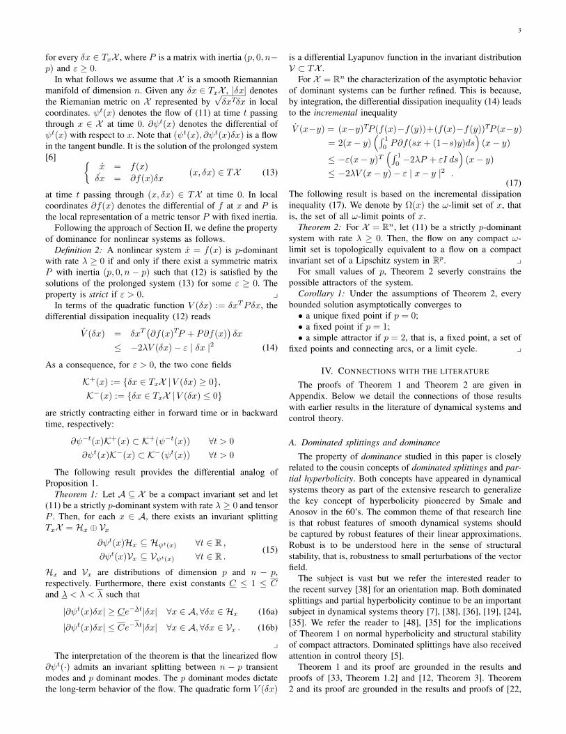
Strictly 1-dominant systems are strictly differentially posi-tive systems [12], [9]. The contractive cone K− is an ellip-soidal cone, that is, it is the union of two solid pointed convexcones K− = −K∗ ∪ K∗as illustrated in Figure 1.

δxTPδx ≤ 0

K∗

δx(0)

δx(t)

Figure 1. For ε > 0 (12) guarantees that any trajectory moves from theboundary of K∗ towards the interior.

A linear system that contracts a solid pointed convex cone isa positive system [27], [4]. Differential positivity thus inducesa dominated splitting between one dominant direction andn − 1 dominated directions. The reader is referred to [12],[9] for a comprehensive analysis of the asymptotic behaviorof differentially positive systems.

The distinction between 1-dominance and differential pos-itivity is again the property of projective contraction versus

vertical contraction. Differential positivity does not implycontraction in the 1-dimensional vertical subspace Vx. As aconsequence, the statement of Corollary 1 for p = 1 only holdsfor generic initial conditions of strictly differentially positivesystems, see [12, Corollary 5].

For X = Rn, 1-dominance is also tightly related to mono-tonicity [40], [21], [1], [22]. A monotone system preserves apartial order : any pair of trajectories x(·), y(·) from orderedinitial conditions x(0) y(0) satisfy x(t) y(t) for all t ≥ 0.

Monotonicity is implied by 1-dominance. The partial orderis the usual partial order associated to a pointed convexcone: x y iff y − x ∈ K∗. Monotonicity requires thattrajectories y(0) − x(0) ∈ K∗ satisfy y(t) − x(t) ∈ K∗for all t ≥ 0, which is guaranteed by 1-dominance by theinvariance V (x(t) − y(t)) ≤ 0 for all t ≥ 0 and by the factthat if x(0) − y(0) = 0 then x(t) − y(t) = 0, for all t ≥ 0.Here also, monotonicity is independent of λ. The assumptionλ ≥ 0 makes 1-dominance stronger than monotonicity andthe statement of Corollary 1 for p = 1 only holds for genericinitial conditions of monotone systems, see [18], [22].

D. Contraction of rank 2 cones and 2-dominance

The property of 2-dominance provides the following gener-alization of Poincare-Bendixson theorem:

Corollary 2: For p = 2, under the assumptions of Theorem2, let U ⊆ X be a compact forward invariant set that does notcontain fixed points. Then, the ω-limit set of any point in Uis a closed orbit. y

Proof: Take any ω-limit set contained in U . By Theorem2 the flow restricted to this set is topologically equivalent tothe flow of a planar system. By Poincare-Bendixson theorem[20, Chapter 11, Section 4], a nonempty compact limit set of aplanar system which contains no fixed points is a closed orbit.

A similar generalization was developped in the papers [41],[42], [39] by generalizing the concept of monotonicity to rank-2 cones. It is this generalization that motivated the resultsin the present paper. Note that the satement of Corollary 2only holds for generic initial conditions of rank 2 monotonesystems. The stronger conclusion of Corollary 2 is again dueto the assumption of a nonnegative dissipation rate λ ≥ 0.

E. Invariant cone fields

The assumption of a constant matrix P makes the conefields K+(x) and K−(x) constant, that is, the same cone isattached to every x ∈ X . A more intrinsic characterizationfor X = Rn is that the cone field is invariant by translation,the natural group action on a vector space. This geometricinterpretation allows for extensions on Lie groups and, moregenerally, homogeneous spaces [29], [30], [3]. The definitionof dominance thus assumes an invariant cone field in thepresent paper. The invariance of the cone field is an importantsource of tractability for the search of the storage.

5

V. ALGORITHMIC TEST FOR p-DOMINANCEAND A SIMPLE EXAMPLE

A. Dominant spectral splitting

A necessary condition for dominance is that the spectrum ofthe family of matrices ∂f(x) + λI , x ∈ X , admits a uniformsplitting, see Figures 2 (left) and 3 (left) for an illustration.

Theorem 3: Let (11) be a strictly p-dominant system. Then,there exists a maximal interval (λmin, λmax) such that ∂f(x)+λI has p unstable eigenvalues and n − p stable eigenvalues(negative real part) for each λ ∈ (λmin, λmax), for every x ∈X . y

Spectral analysis of the Jacobian matrix ∂f(x) is thus usefulto select p and λ in dominance analysis. The uniform splittingof the spectrum is necessary but of course not sufficientfor dominance. This is well-known even for p = 0. Forinstance, classical counterexamples to Kalman’s conjecture[23] illustrate that a system can fail to be contractive evenwhen the spectrum of its Jacobian is uniformly in the left halfcomplex plane.

B. Convex relaxations

Sufficient conditions for dominance are provided by theinequality

∂f(x)TP + P∂f(x) + 2λP + εI ≤ 0 ∀x ∈ X (18)

whose solutions P , for some ε ≥ 0, must also satisfy a fixedinertia constraint.

If the spectrum of ∂f(x) admits a stable splitting for a givenλ, then all the solutions P of (18) must share the same inertia,meaning that the inertia condition can be dropped. One is thenleft with solving an infinite family of LMIs.

It is common practice to reduce an infinite family ofLMIS to a finite family through convex relaxation. LetA := A1, . . . , AN be a family of matrices such that∂f(x) ∈ ConvexHull(A) for all x. Then, by construction,any (uniform) solution P to

ATi P + PAi + 2λP + εI ≤ 0 1 ≤ i ≤ N (19)

is a solution to (18). For instance, at each x,∂f(x) =

∑Ni=1 ρi(x)Ai for a given set of ρi(x) such

that∑Ni=1 ρi(x) = 1. Thus, the left-hand side of (18) reads(∑N

i=1 ρi(x)ATi

)P + P

(∑Ni=1 ρi(x)Ai

)+ 2λP + εI =∑N

i=1 ρi(x)(ATi P + PAi + 2λP + εI

)≤ 0, where the last

inequality follows from (19).The algorithmic steps of dominance analysis of a given

nonlinear system x = f(x) can thus be summarized asfollows:

1) Estimate p and λ from the spectrum analysis of ∂f(x)2) Reduce the infinite family of LMIs to a finite family by

convex relaxations.3) Test the feasability of the relaxed LMI with a LMI

solver.

C. Example

We illustrate the theory on a classical textbook example:a one degree of freedom mechanical system with nonlinearspring (Duffing model), actuated by a DC motor with aPI feedback control. While this example is elementary, itillustrates the tractability of dominance analysis on a four-dimensional model, for which a global analysis of the attrac-tors is a nontrivial problem.

The mechanical model is given by

xp = xv xv = −α(xp)− cxv + u (20)

where xp and xv are position and velocity of the massrespectively, u is the force input to the system, c is the dampingcoefficient, and α(xp) := ∂U(xp) is the force deriving fromthe mechanical potential U : R → R. Contraction, or 0-dominance is expected with sufficient damping if the potentialis strictly convex. A differential quadratic storage is easilyfound for the numerical value c = 5 and the assumption

1 ≤ ∂α(xp) ≤ 5 .

P is computed via convex relaxation (19) for A1 :=[

0 1−1 −5

]and A2 :=

[0 1−5 −5

]. For λ = 0 and ε = 0.01, the LMI solver

(Yalmip [25]) returns

P :=

[0.8696 0.14820.1482 0.1304

].

which is positive definite.The same approach is repeated for the non-convex potential

−2 ≤ ∂α(xp) ≤ 5 ,

which allows for several minima (including the classicaldouble-well potential of the nonlinear Duffing model [17]).Figure 2 (left) suggests a stable splitting between the twoeigenvalues. The differential storage is computed again byconvex relaxation (19) for A1 :=

[0 12 −5

]and A2 :=

[0 1−5 −5

].

For λ = 2 and ε = 0.01, the LMI solver returns

P =

[−5.1987 3.62603.6260 6.1987

].

which has inertia (1, 0, 1). Figure 2 (right) shows the nonpositive level sets of δxTPδx. The system is 1-dominant,meaning that every bounded trajectory asymptotically con-verges to some fixed point.

Suppose now that the mechanical system is driven by a DCmotor modelled by the electrical equation

u = kfxi Lxi = −Rxi − kexv + V . (21)

xi is the current of the circuit, kf is a static approximationof the current to force characteristic, L and R are inductanceand resistance respectively, ke is the back electromotive forcecoefficient, and the voltage V is an additional input.

It is easy to verify that 1-dominance is preserved for R = 1,kf = 1, ke = 1, and 0 < L < 0.05, since the time-scale sepa-ration between electrical and mechanical dynamics introducesa mild perturbation on the dominant/slow dynamics of thesystem. For L = 0.1 the reduced time scale separation allowsfor interaction between electrical and mechanical dynamics.

6

-6 -4 -2 0Re

-2.5

-2

-1.5

-1

-0.5

0

0.5

1

1.5

2

2.5

Im

-1 -0.5 0 0.5 1/ x

1

-1

-0.8

-0.6

-0.4

-0.2

0

0.2

0.4

0.6

0.8

1

/ x 2

Figure 2. Left: roots of the Jacobian of the mechanical systems for differentxp. The value of λ is emphasized by the vertical dashed line. Right: negativelevel sets of δxTPδx where P has inertia (1, 0, 1).

The distribution of the eigenvalues of the Jacobian in Figure 3(left) suggests that strict 1-dominance still holds. Indeed, forL = 0.1, λ = 2, and ε = 0.01, the LMI solver returns

P =

−3.0942 0.8985 −0.53550.8985 3.3771 0.1935−0.5355 0.1935 0.7171

.which has inertia (1, 0, 2). For constant inputs V , everybounded trajectory necessarily converges to some fixed point,as illustrated in Figure 3 (right), where we considered thedouble well potential U(xp) := x2p/4 + cos(xp).

-10 -5 0Re

-2

-1

0

1

2

Im

0 50 100t

0

0.5

1

1.5

2

x p

Figure 3. Left: roots of the Jacobian of (20) and (21), by sampling −2 ≤∂α(xp) ≤ 5 at different xp. Right: Trajectory of the mass position in timefor the interconnected system (20), (21) with potential U(xp) := x2p/4 +cos(xp), from the initial condition xp = 0.05, xv = 0, xi = 0, at constantV = 0.

Finally, we close the loop with a PI controller

V = kP (r − xp) + kIxc xc = r − xp (22)

where xc is the integrator variable, kP and kI are proportionaland integral gains, respectively, and r is the reference.

The degree of dominance of the closed loop can be mod-ulated via PI control. A detailed analysis of PI control for p-dominance is beyond the scope of this paper. We just observethat with gains kP = 1 and kI = 5 the eigenvalues of theJacobian in Figure 4 (left) exhibits a stable splitting into twogroups of two eigenvalues. 2-dominance is verified with λ = 2,

ε = 0.01, in which case the LMI solver returns the storage

P =

−4.3713 1.7901 −0.5507 0.02161.7901 5.6483 0.3768 −0.9320−0.5507 0.3768 1.0521 −0.43630.0216 −0.9320 −0.4363 −1.3291

.

with inertia 2, 0, 2). For r = 0 the unique fixed point at 0is unstable. We conclude that every bounded trajectory mustconverge to a periodic orbit, as illustrated in Figure 4 (right).

-10 -5 0Re

-2

-1

0

1

2

Im

0 50 100 150 200t

-3

-2

-1

0

1

2

3

x p

Figure 4. Left: roots of the Jacobian of the closed loop given by (20), (21)and (22) by sampling −2 ≤ ∂α(xp) ≤ 5 at different xp. Right: Trajectoryof the mass position in time for the closed loop (20), (21), (22) with potentialU(xp) := x2p/4 + cos(xp) and PI control gains kP = 1 and kI = 5, fromthe initial condition xp = 0.05, xv = 0, xi = 0 and xc = 0, at constantr = 0.

Remark 1: A variant of the example is to replace themechanical model with the nonlinear pendulum xp = xv ,xv = − sin(xp) − cxv + u with (xp, xv) ∈ S × R. One-dominance is proven as in Duffing example but the state-space is now nonlinear. From Theorem 1, every attractor ofthe pendulum exhibits at least one direction of contraction,locally. The shape of S × R makes 1-dominance compatiblewith fixed point attractors, for small constant torque u, andwith attractors defined by periodic orbits, for large constanttorque u, [44, Section 8.5]. See also the analysis in [12] usingdifferential positivity. y

VI. INTERCONNECTIONS

A. Differential dissipativity theory

Dissipativity theory is a fundamental complement to stabil-ity theory in systems and control [49], [50], [51]. Stability,and more generally, dominance, is the property of a closedsystem. Dissipativity is the property of an open system, i.e.a system with inputs and outputs. By decomposing a closedsystem as an interconnection of open subsystems, the searchof quadratic storage for the analysis of the closed system isconverted into the solution of linear matrix inequalities for theopen subsystems.

The recent papers [10], [14], [46] have proposed to use dis-sipativity theory differentially in order to study contraction (i.e.0-dominance) via interconnections. We pursue this approachto study p-dominance. We restrict to open systems of the form

x = f(x) +Buy = Cx+Du

x ∈ X , (y, u) ∈ W (23)

7

where X and W are smooth manifolds of dimension n andm, respectively. The associated prolonged system reads

x = f(x) +Bu˙δx = ∂f(x)δx+Bδuy = Cx+Duδy = Cδx+Dδu

(24)

where (x, δx) ∈ TX and (w, δw) := ((y, u), (δy, δu)) ∈ TW .We also assume that W is covered by a single chart and

that the matrix L and the symmetric matrices Q and R belowhave suitable dimensions. All restrictions above relate to therestriction of constant tensors P in this paper for the analysisof dominance.

Definition 3: A nonlinear system (23) is differentially p-dissipative with rate λ and differential supply rate

s(w, δw) :=

[δyδu

]T[Q LLT R

][δyδu

](25)

if for some symmetric matrix P with inertia (p, 0, n− p) andsome constant ε ≥ 0, the prolonged system (24) satisfies theconic constraint[

˙δxδx

]T[0 PP 2λP+εI

][˙δxδx

]≤[δyδu

]T[Q LLT R

][δyδu

](26)

for all (x, δx) ∈ TX and all (w, δw) ∈ W . (23) is strictlydifferentially p-dissipative if ε > 0. y

Differential dissipativity is guaranteed by the feasibility ofthe inequality[∂f(x)TP+P∂f(x)−CTQC+2λP+εI PB−CTL− CTQD

BTP−LTC −DTQC −R−DTL−LTD−DTQD

]≤0

for some symmetric matrix P with inertia (p, 0, n − p) andsome constant ε ≥ 0. A necessary condition for the feasibilityof this inequality is that ∂f(x)TP+P∂f(x)−CTQC+2λP+εI ≤ 0 which corresponds to (18) for Q = 0 and clarifies theconnection between differential dissipativity and dominance.This infinite family of LMIs can reduced to a finite familythrough relaxations, following the approach in Section V-B.

B. A dissipativity theorem for p-dominance

Suppose that a nonlinear system can be decomposed as theinterconnection of two subsystems:

x1 = f1(x1) +B1u1y1 = Cx1 +D1u1

(27a)x2 = f2(x2) +B2u2y2 = Cx2 +D2u2

(27b)

u = Hy + v (27c)

where the matrix H specifies the interconnection patternbetween inputs u = [uT1 uT2 ]T and outputs y = [ yT1 yT2 ]T .v = [ vT1 vT2 ]T is an additional input. Then the dissipativitytheorem below provides conditions for the differential p-dissipativity of the interconnected system from the differentialp-dissipativity of its components.

The formulation of the theorem follows the approach of[31]. The theorem can be easily adapted to the interconnec-tion of several systems [32]. In what follows we will use

Q :=[Q1

Q2

], L :=

[L1

L2

], and R :=

[R1

R2

]for readability,

where for i ∈ 1, 2 the matrices Qi, Li and Ri characterizethe differential supply rate fo each subsystem.

Theorem 4: Let (27a) and (27b) be (strictly) differentiallyp1-dissipative and p2-dissipative respectively, with uniformrate λ and differential supply rate[

δyδu

]T[Qi LiLTi Ri

] [δyδu

]i ∈ 1, 2 . (28)

Then, the interconnected system (27) is (strictly) differentiallyp-dissipative with degree p = p1 + p2, rate λ, and differentialsupply rate [

δyδv

]T[Q LLT R

] [δyδv

](29)

where

Q := Q+ LH +HT LT +HT RHL := L+HT RR := R .

(30)

For v = 0, the interconnected system (27) is (strictly) p-dominant if Q ≤ 0. y

Theorem 4 is a general result to study dominance viainterconnections. In particular, it provides an interconnectiontheorem for the analysis of contraction (0-dominance) andmonotonicity (1-dominance).

C. Differential passivity analysis

The passivity supply[δyδu

]T[0 II 0

][δyδu

](31)

plays an important role in dissipativity theory because itconnects the theory to the physical property that a passivesystem can only store the energy supplied by its environment.The theory of port-Hamiltonian systems encompasses a broadmodeling framework of physical models with passivity prop-erties [47].

The passivity theorem states that the feedback interconnec-tion of passive systems is passive. A differential version ofthis important theorem is provided by Theorem 4: any systemthat is differentially p-passive preserves that property underthe feedback interconnection with a differentially passive (i.e.0-passive) system.

Passivity theory has proven useful in identifying robust con-troller structures that preserve stability. An important particularcase is the class of proportional-integral controllers, that wenow revisit in the light of dominance analysis.

We first consider the proportional feedback controller

(P ) y = kP (u) . (32)

The controller is differentially 0-passive (for arbitrary non-negative rate) from u to y provided that the mapping kp(·)is monotone, or differentially positive: ∂kP (u) ≥ 0 for allu ∈ R. For instance,[

δyδu

]T[0 II 0

][δyδu

]= 2δuT∂k(u)δu ≥ 0.

8

Likewise, the proportional-integral feedback controller

(PI) xc = u, y = kP (u) + kIxc (33)

from u to y is• differentially 0-passive if kP (·) is monotone and if kI ≥

0, with rate λ = 0.• differentially 1-passive if kP (·) is monotone and if kI <

0, with rate λ ≥ 0 (strictly for λ > 0).This is because the storage S(δxc) := kI

2 δx2c satisfies S ≤

δuδy. Furthermore, for λ > 0 and kI < 0 we have S +λkIδx

2c + εδx2c ≤ δuδy for ε = λ|kI |.

As an illustration, we revisit the nonlinear (Duffing) mass-spring-damper system in Section V-C. For any nonlinear springsatisfying −3 ≤ ∂α(xp) ≤ 3, the system is strictly differential1-passive with rate λ = 2 from u to y = −xp: defining thestate x := [xp xv ], the variational dynamics ˙δx = A(x)δx+Bδu, δy = Cδx

A(x) :=

[0 1

−∂α(xp) −5

]B :=

[01

]C :=

[−1 0

].

satisfiesA(x)TP + PA(x) + 2λP + εI ≤ 0

PB = CT

for P =[−2 −1−1 0

]and ε = 0.01, for all x ∈ R2.

Assume for simplicity that kP (·) is odd and monotone andconsider the interconnection

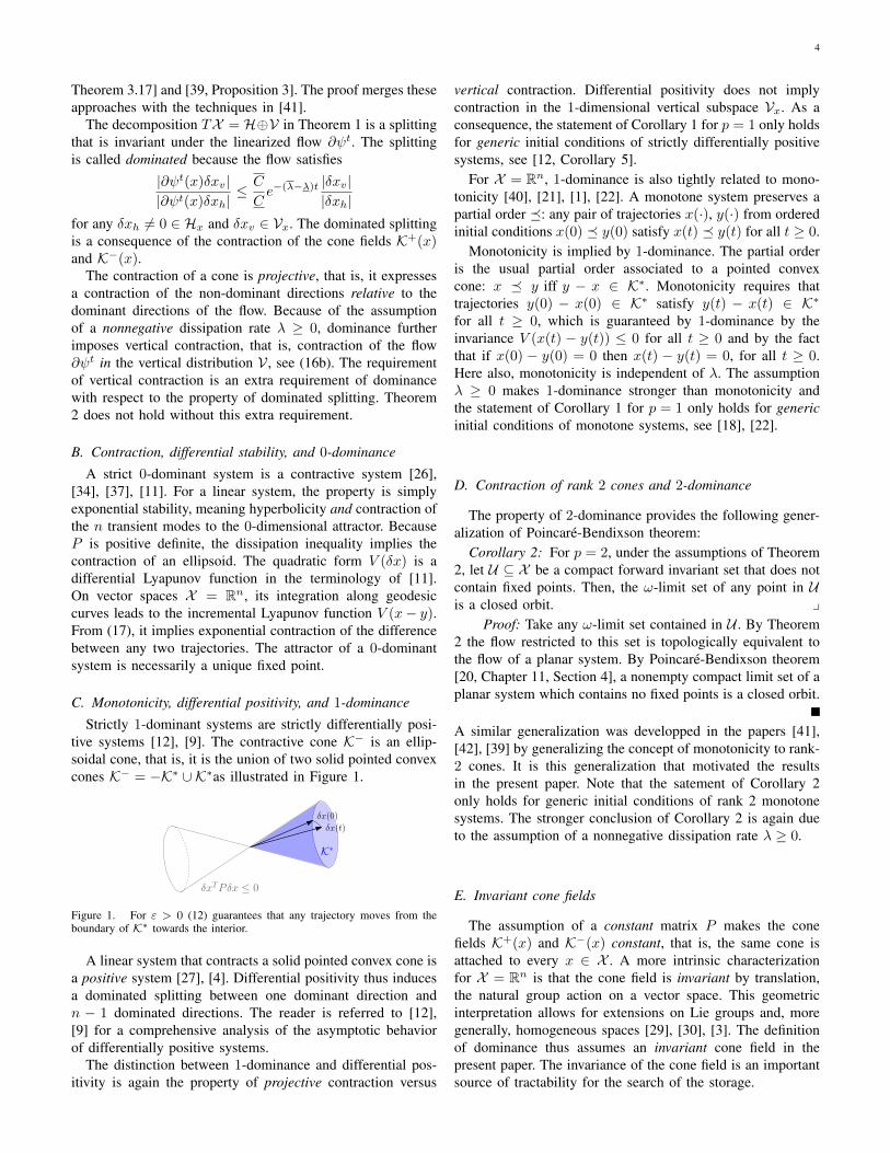
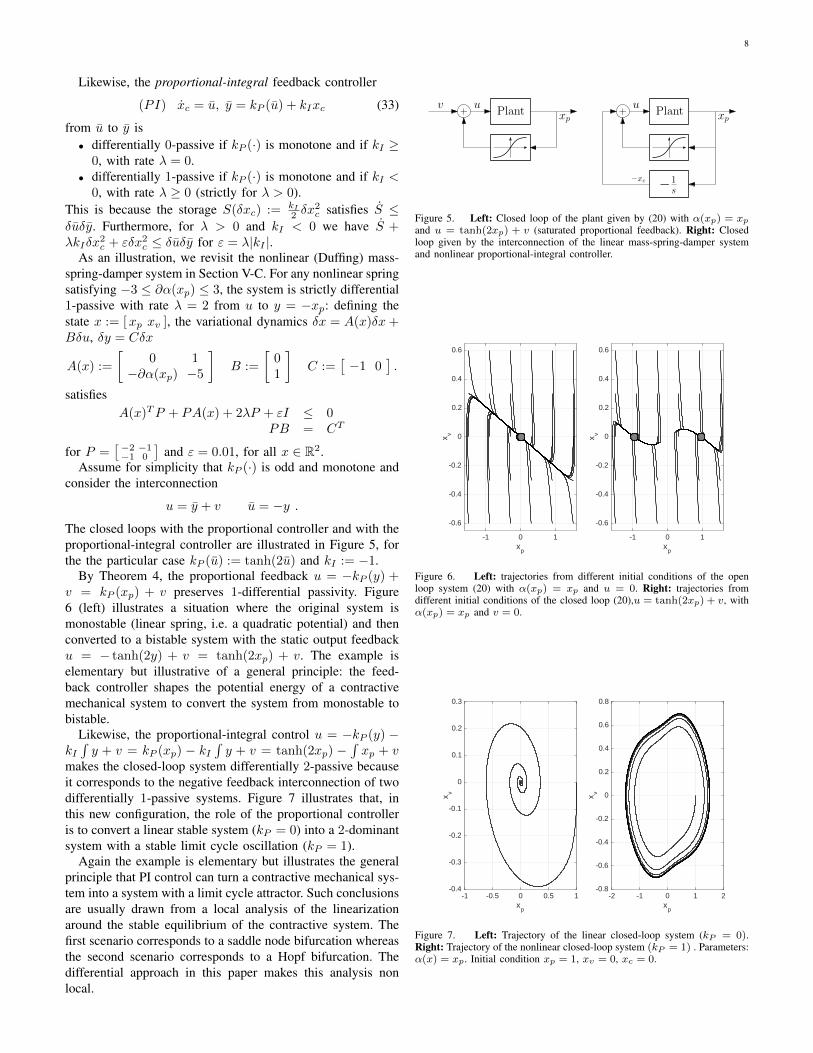
u = y + v u = −y .The closed loops with the proportional controller and with theproportional-integral controller are illustrated in Figure 5, forthe the particular case kP (u) := tanh(2u) and kI := −1.

By Theorem 4, the proportional feedback u = −kP (y) +v = kP (xp) + v preserves 1-differential passivity. Figure6 (left) illustrates a situation where the original system ismonostable (linear spring, i.e. a quadratic potential) and thenconverted to a bistable system with the static output feedbacku = − tanh(2y) + v = tanh(2xp) + v. The example iselementary but illustrative of a general principle: the feed-back controller shapes the potential energy of a contractivemechanical system to convert the system from monostable tobistable.

Likewise, the proportional-integral control u = −kP (y) −kI∫y + v = kP (xp) − kI

∫y + v = tanh(2xp) −

∫xp + v

makes the closed-loop system differentially 2-passive becauseit corresponds to the negative feedback interconnection of twodifferentially 1-passive systems. Figure 7 illustrates that, inthis new configuration, the role of the proportional controlleris to convert a linear stable system (kP = 0) into a 2-dominantsystem with a stable limit cycle oscillation (kP = 1).

Again the example is elementary but illustrates the generalprinciple that PI control can turn a contractive mechanical sys-tem into a system with a limit cycle attractor. Such conclusionsare usually drawn from a local analysis of the linearizationaround the stable equilibrium of the contractive system. Thefirst scenario corresponds to a saddle node bifurcation whereasthe second scenario corresponds to a Hopf bifurcation. Thedifferential approach in this paper makes this analysis nonlocal.

Plantu

xp+

−xc −1s

Plantu

xpv

+

Figure 5. Left: Closed loop of the plant given by (20) with α(xp) = xpand u = tanh(2xp) + v (saturated proportional feedback). Right: Closedloop given by the interconnection of the linear mass-spring-damper systemand nonlinear proportional-integral controller.

-1 0 1x

p

-0.6

-0.4

-0.2

0

0.2

0.4

0.6

x v

-1 0 1x

p

-0.6

-0.4

-0.2

0

0.2

0.4

0.6

x v

Figure 6. Left: trajectories from different initial conditions of the openloop system (20) with α(xp) = xp and u = 0. Right: trajectories fromdifferent initial conditions of the closed loop (20),u = tanh(2xp) + v, withα(xp) = xp and v = 0.

-1 -0.5 0 0.5 1x

p

-0.4

-0.3

-0.2

-0.1

0

0.1

0.2

0.3

x v

-2 -1 0 1 2x

p

-0.8

-0.6

-0.4

-0.2

0

0.2

0.4

0.6

0.8

x v

Figure 7. Left: Trajectory of the linear closed-loop system (kP = 0).Right: Trajectory of the nonlinear closed-loop system (kP = 1) . Parameters:α(x) = xp. Initial condition xp = 1, xv = 0, xc = 0.

9

D. Differential small gain analysis

The supply [δyδu

]T[ −I 00 γ2I

][δyδu

]. (34)

also has a special status in dissipativity theory because of itsconnection to the small gain theorem, a cornerstone of robustcontrol theory [53], [52], [8], [54], [45].

When specialized to the supply (34), Theorem 4 provides adifferential version of the small gain theorem: p-dominance ispreserved under feedback with a 0-dominant system providedthat their finite differential gains γ1 and γ2 (of degree p and0 respectively) satisfy the small gain condition γ1γ2 < 1.

The differential small gain theorem opens the way to adifferential approach of nonlinear robust control. The link withan operator-theoretic definition of the differential gain of adominant system is beyond the scope of this paper (see e.g.[16] for a concept of differential gain for stable systems), butwe briefly illustrate how the theorem can be used in nonlinearrobustness analysis.

∆

+r v yNominalclosed loop

Figure 8. A nonlinear plant with parametric uncertainties represented as thefeedback interconnection of nominal plant and uncertain dynamics ∆.

Consider them nominal closed loop in Figure 5 (right)where the mass-spring-damper system (20) with linear springα(xp) = xp is interconnected to a saturated proportional-integral feedback u = tanh(2xp) −

∫xp + v. We study the

robustness of the oscillations to perturbations affecting thespring constant and damping coefficient. We use the usualrepresentation of parametric uncertainties through feedbackinterconnections as shown in Figure 8.

For c = 5 and λ = 2 the nominal closed loop system is2-dominant with differential gain γ := 0.5636 from the inputv to the position output xp, obtained for

P :=

−0.5522 0.0498 −0.01710.0498 1.4946 0.3068−0.0171 0.3068 0.0576

.Nonlinear perturbations on the mechanical spring of the form

α(xp) = xp + ∆(xp)

are captured by the feedback interconnection in Figure 8,taking v = ∆(xp). The differential small-gain theorem impliesthat 2-dominance is preserved for any |∂∆(xp)| ≤ 1/γ.Furthermore, for any perturbation ∆(xp) that preserves theorigin as a unique and unstable fixed point of the closed loopsystem, every bounded trajectory of the perturbed closed loopwill converge to a periodic orbit, like in the nominal case.

The analysis of perturbations affecting the damping coeffi-cient c = 5 is similar. For c = 5 and λ = 2 the nominal closed

loop system is 2-dominant with differential gain γ := 0.5468from the input v to the velocity output xv , obtained for

P :=

−0.2859 −0.0028 −0.0131−0.0028 1.2328 0.2977−0.0131 0.2977 0.0532

.Therefore oscillations will persist when the linear dampingcoefficient cxv is replaced by a nonlinear coefficient c(xv)given by

c(xv) = 5xv + ∆(xp)

provided that |∆(xv)| < 1/γ and that the origin remains anunstable fixed point.

VII. CONCLUSION

This paper illustrated that linear-quadratic dissipativity the-ory, a cornerstone of stability theory, generalizes with surpris-ing ease to the analysis of dominance. Dominance analysisin turn is relevant to capture the frequent property that theasymptotic behavior of a nonlinear dynamical model is low-dimensional. In particular, the theory seems relevant to gen-eralize the theory of stability to a theory of multistability andlimit cycle analysis.

The approach in this paper is differential, meaning that theusual linear matrix inequalities of dissipativity theory are con-sidered in the tangent bundle. They characterize a dominatedsplitting of the linearized flow between p dominant directionsand n− p transient directions. This property is captured withthe usual linear matrix inequalities of dissipativity theory, withthe only difference that the solution matrix P is required tohave a fixed inertia (p negative eigenvalues and n−p positiveeigenvalues), the standard stability framework correspondingto the case p = 0.

An important restriction throughout this paper is to analyzep-dominance with a constant quadratic storage (i.e. a constantP ). This restriction is the price to be paid for tractability.Standard LMI solvers can then be used to construct the storage.

A number of generalizations deserve further attention.Those include the construction of differential storages thatare non quadratic, or/and state-dependent (i.e. non constantP (x)), as well as the study of dominance with state-dependentrate λ(x), or systems with a different degree of dominance indifferent parts of the state-space, or the analysis of dominancein non smooth systems. Such generalizations have receivedconsiderable attention in the analysis of contraction, i.e. 0-dominance, suggesting clear avenues to study p-dominance.Finally, differential dissipativity theory offers an opportunity torevisit classical results from robust control theory and absolutestability theory in the context of multistable and oscillatorysystems, see e.g. [28] for a first step in that direction.

APPENDIX

Proof of Theorem 1.Invariant splitting. For any p > 0 and for any δx ∈ K−, the

dissipation inequality (14) implies

V (δx) ≤ −2λV (δx)− ε | δx |2≤ −ε | δx |2 (35)

10

for all x ∈ X and all δx on the boundary of K−, whichguarantees that

∀t ≥ 0 : ∂ψtK− ⊆ K− (36a)∀t > 0 : ∂ψt(K− \ 0) ⊂ K−. (36b)

The dissipation inequality (14) also implies

V (δx) ≤ −2λV (δx)− ε | δx |2≤ −(2λ− ε1)V (δx) (37)

for ε1 := ε|λmin(P )| > 0. Time-integration of this inequality

yields the estimate

∀t ≥ 0 :e2λtV (∂ψtδx)

V (δx)≥ eε1t (38)

which holds uniformly for all x ∈ X and all δx in the interiorof K−. (36) and (38) guarantee that there exist T > 0 andµ > 1 such that |e

λt∂ψtδx||δx| ≥ µ for all t ≥ T , all x ∈ X and

all δx ∈ K−.Likewise, for any n − p > 0 and for any δx ∈ K+, the

dissipation inequality (14) implies

V (δx) ≤ −2λV (δx)− ε | δx |2≤ −(2λ+ ε2)V (δx) (39)

for ε2 = ελmax(P ) > 0. Integration of the first inequality

backward time guarantees that

∀t ≥ 0 : ∂ψ−tK+ ⊆ K+ (40a)

∀t > 0 : ∂ψ−t(K+ \ 0) ⊂ K+. (40b)

Integration of the second inequality backward time also yieldsthe estimate

∀t ≥ 0 :e−2λtV (∂ψ−tδx)

V (δx)≥ eε2t (41)

which holds uniformly for all x ∈ X and all δx in the interiorof K+. As above, (40) and (41) guarantee that there existT > 0 and µ > 1 such that |e

−λt∂ψ−tδx||δx| ≥ µ for all t ≥ T ,

all x ∈ X and all δx ∈ K+.From here, we proceed as in the proof of [33, Theorem 1.2]

(see also [2, Chapter 3]) to show that

Hx :=⋂t≥0 e

λt∂ψt(x)K−(ψ−t(x)) ⊂ K−(x)

Vx :=⋂t≥0 e

−λt∂ψ−t(ψt(x))K+(ψt(x)) ⊂ K+(x)

are invariant distributions of dimension p and n − p respec-tively, that is,

eλt∂ψt(x)Hx ⊆ Hψt(x) ∀t ∈ R ,

eλt∂ψt(x)Vx ⊆ Vψt(x) ∀t ∈ R .

Since eλt is just a scalar factor, (15) follows.Exponential estimates. Observe that δx ∈ H implies that

δx belongs to the interior of K−. The estimate (16a) withλ = λ − ε1

2 follows from the fact that −V (δx) is positivedefinite in H and that V (δx) satisfies (37). For instance, thereexist 0 < ρ1 ≤ ρ2 such that ρ1δxTδx ≤ −V (δx) ≤ ρ2δx

Tδxfor all δx ∈ H and (37) gives ρ2|∂ψtδx|2 ≥ −V (∂ψtδx) ≥−e−(2λ−ε1)tV (δx) ≥ e−(2λ−ε1)tρ1|δx|2 for all t ≥ 0, fromwhich (16a) follows.

Likewise, δx ∈ V implies that δx belongs to the interior ofK+. The estimate (16b) with λ = λ + ε2

2 follows from the

fact that V (δx) is positive definite in V and satisfies (39).

Proof of Theorem 2. From the dissipation inequality (17) wederive the inequality d

dte2λtV (x−y) = e2λtV +2λe2λtV (x−

y) ≤ −e2λtε | x − y |2 which, by time integration, impliesthe following estimate for any pair of solutions initialized atx0, y0 ∈ X :

∀t ≥ 0 : V (ψt(x0)− ψt(y0)) ≤ e−2λtV (x0 − y0)−

−ε∫ t

0

e2λ(τ−t)|ψτ(x0)− ψτ(y0)|2dτ (42)

For large t ≥ 0, the first term on the right hand side vanishes.This implies that the difference between any two solutionseither asymptotically vanishes or eventually remains in thecone K−. We conclude that if x and y are distinct ω-limitpoints, then necessarily V (x− y) < 0.

Consider any compact set Ω of ω-limit points. Let HP andVP the invariant subspaces of the matrix P associated to thep negative and n−p positive eigenvalues, respectively. Definethe linear projection Π : X → HP parallel to VP . We claimthat Π restricted to Ω is one-to-one. This is because x 6= yand Π(x− y) = 0 imply V (x− y) > 0, which was proved tocontradict (42).

The remaining argument follows the proof of [22, Theorem3.17]. If y ∈ ΠΩ(x) then y = Πz for a unique z ∈ Ω(x) andthe flow Πψt(z) on VP is generated by the vector field

F (y) := Πf(Π−1(y)) y ∈ Ω(x) ,

which is Lipschitz by construction. Proof of Theorem 3

By Proposition 1, the feasibility of ∂f(x)TP + P∂f(x) +2λP ≤ −εI , for ε > 0 and for P of inertia (p, 0, n − p)guarantees that each matrix ∂f(x) +λI has p unstable eigen-values and n − p stable eigenvalues (negative real part) ateach x ∈ X . The splitting of the eigenvalues of ∂f(x) ateach x is preserved for every value of λ within some givenspectral gap (λmin(x), λmax(x)). Thus, by the uniformity ofthe strict inequality above, λmin := supx∈X λmin(x) < λ andλmax := infx∈X λmax(x) > λ.

Proof of Theorem 4Let P1 and P2 be solutions to (3) respectively for (27a)

and (27b). Take P := P1 + P2, x := [xT1 xT2 ]T , and δx :=[ δxT1 δxT2 ]T . Note that P1 has inertia (p1, 0, n1− p1) and P2

has inertia (p2, 0, n2−p2), where n1 and n2 are the dimensionsof the two state manifolds, respectively. It follows that P hasinertia (p1 +p2, 0, n1 +n2−p1−p2). Furthermore, by (strict)differential dissipativity of (27a) and (27b), (3) can be writtenin the aggregated form ˙δx

TPδx + δxTP ˙δx + δxT (2λP +

εI)δx ≤ δyTQδy + δyTLδu + δuTLTδy + δuTRδu, for

some ε ≥ (ε > 0). Since δu = Hδy + δv, the expressionabove reads ˙δx

TPδx + δxTP ˙δx + δxT (2λP + εI)δx ≤

δyTQδy+δyTLδv+δvTLT δy+δuTRδu which shows (strict)differential p-dissipativity of the interconnected system.

Finally, for v = 0 we get ˙δxTPδx+δxTP ˙δx+δxT (2λP +

εI)δx ≤ δyTQδy ≤ 0 where the last inequality follows from

11

the condition Q ≤ 0. This shows that P is a solution of (12).

REFERENCES

[1] D. Angeli and E.D. Sontag. Monotone control systems. IEEE Transac-tions on Automatic Control, 48(10):1684 – 1698, 2003.

[2] A. Katok B. Hasselblatt. Handbook of dynamical systems, volume 1A.Elsevier Science, first edition, 2002.

[3] S. Bonnabel, P. Martin, and P. Rouchon. Non-linear symmetry-preserving observers on lie groups. IEEE Transactions on AutomaticControl, 54(7):1709–1713, July 2009.

[4] P.J. Bushell. Hilbert’s metric and positive contraction mappings in aBanach space. Archive for Rational Mechanics and Analysis, 52(4):330–338, 1973.

[5] F. Colonius, L. Grune, and W. Kliemann. The Dynamics of Control.Systems & Control: Foundations & Applications. Birkhauser Boston,2012.

[6] P.E. Crouch and A.J. van der Schaft. Variational and Hamiltoniancontrol systems. Lecture notes in control and information sciences.Springer, 1987.

[7] S. Crovisier and R. Potrie. Introduction to partial hyperbolic dynamics.Technical report, Minicourse, 2015. Minicourse.

[8] C.A. Desoer and M. Vidyasagar. Feedback Systems: Input-OutputProperties, volume 55 of Classics in Applied Mathematics. Societyfor Industrial and Applied Mathematics, 1975.

[9] F Forni. Differential positivity on compact sets. In 54th IEEEConference on Decision and Control, pages 6355–6360, 2015.

[10] F. Forni and R. Sepulchre. On differentially dissipative dynamicalsystems. In 9th IFAC Symposium on Nonlinear Control Systems, 2013.

[11] F. Forni and R. Sepulchre. A differential Lyapunov framework for con-traction analysis. IEEE Transactions on Automatic Control, 59(3):614–628, 2014.

[12] F. Forni and R. Sepulchre. Differentially positive systems. IEEETransactions on Automatic Control, 61(2):346–359, 2016.

[13] F. Forni and R. Sepulchre. A dissipativity theorem for p-dominantsystems. In 56th IEEE Conference on Decision and Control, 2017.

[14] F. Forni, R. Sepulchre, and A.J. van der Schaft. On differential passivityof physical systems. In 52nd IEEE Conference on Decision and Control,2013.

[15] V. Fromion and G. Scorletti. Connecting nonlinear incremental Lya-punov stability with the linearizations Lyapunov stability. In 44th IEEEConference on Decision and Control, pages 4736 – 4741, December2005.

[16] T.T. Georgiou. Differential stability and robust control of nonlinearsystems. Mathematics of Control, Signals and Systems, 6(4):289–306,1993.

[17] J. Guckenheimer and P. Holmes. Nonlinear oscillations, dynamicalsystems, and bifurcations of vector fields. Springer-Verlag ,New York,Berlin, Heidelberg, Tokyo, page 0, 1986.

[18] M.W. Hirsch. Stability and convergence in strongly monotone dynamicalsystems. Journal fur die reine und angewandte Mathematik, 383:1–53,1988.

[19] M.W. Hirsch, C.C. Pugh, and M. Shub. Invariant Manifolds. LectureNotes in Mathematics 583. Springer Berlin Heidelberg, 1977.

[20] M.W. Hirsch and S. Smale. Differential Equations, Dynamical Systems,and Linear Algebra (Pure and Applied Mathematics, Vol. 60). AcademicPress, 1974.

[21] M.W. Hirsch and H.L. Smith. Competitive and cooperative systems: Amini-review. In L. Benvenuti, A. Santis, and L. Farina, editors, PositiveSystems, volume 294 of Lecture Notes in Control and InformationScience, pages 183–190. Springer Berlin Heidelberg, 2003.

[22] M.W. Hirsch and H.L. Smith. Monotone dynamical systems. InP. Drabek A. Canada and A. Fonda, editors, Handbook of DifferentialEquations: Ordinary Differential Equations, volume 2, pages 239 – 357.North-Holland, 2006.

[23] R.E. Kalman. Physical and mathematical mechanisms of instability innonlinear automatic control systems. Transactions of ASME, 79(3):553–566, 1957.

[24] A. Katok and B. Hasselblatt. Introduction to the Modern Theory ofDynamical Systems. Encyclopedia of Mathematics and its Applications.Cambridge University Press, 1997.

[25] J. Lofberg. Yalmip : a toolbox for modeling and optimization in Matlab.In IEEE International Symposium on Computer Aided Control SystemsDesign, pages 284–289, 2004.

[26] W. Lohmiller and J.E. Slotine. On contraction analysis for non-linearsystems. Automatica, 34(6):683–696, June 1998.

[27] D.G. Luenberger. Introduction to Dynamic Systems: Theory, Models,and Applications. Wiley, 1 edition, 1979.

[28] F.A. Miranda-Villatoro, F. Forni, and R. Sepulchre. Analysis of Lur’edominant systems in the frequency domain. submitted to Automatica,https://arxiv.org/abs/1710.01645, 2017.

[29] C. Mostajeran and R. Sepulchre. Invariant differential positivity andconsensus on lie groups. IFAC-PapersOnLine, 49(18):630 – 635, 2016.10th IFAC Symposium on Nonlinear Control Systems NOLCOS 2016.

[30] C. Mostajeran and R. Sepulchre. Differential positivity with respect tocones of rank k. In 20th IFAC World Congress, 2017.

[31] P. Moylan. Dissipative systems and stability. Lecture Notes incollaboration with D. Hill, University of Newcastle, www.pmoylan.org,2014.

[32] P. Moylan and D. Hill. Tests for stability and instability of interconnectedsystems. IEEE Transactions on Automatic Control, 24(4):574–575,1979.

[33] S. Newhouse. Cone-fields, domination, and hyperbolicity. In Press,editor, Modern Dynamical Systems and Applications, pages 419–432,2004.

[34] A. Pavlov, N. van de Wouw, and H. Nijmeijer. Uniform OutputRegulation of Nonlinear Systems: A Convergent Dynamics Approach.Systems & Control: Foundations & Applications. Birkhauser, 2005.

[35] Y.B. Pesin. Lectures on Partial Hyperbolicity and Stable Ergodicity.Zurich lectures in advanced mathematics. European Mathematical Soci-ety, 2004.

[36] J.F. Plante. Anosov flows. American Journal of Mathematics, 94(3):pp.729–754, 1972.

[37] G. Russo, M. Di Bernardo, and E.D. Sontag. Global entrainment oftranscriptional systems to periodic inputs. PLoS Computational Biology,6(4):e1000739, 04 2010.

[38] M. Sambarino. A (short) survey on Dominated Splitting. ArXiv e-prints,2014.

[39] L.A. Sanchez. Cones of rank 2 and the Poincare–Bendixson propertyfor a new class of monotone systems. Journal of Differential Equations,246(5):1978 – 1990, 2009.

[40] H.L. Smith. Monotone Dynamical Systems: An Introduction to theTheory of Competitive and Cooperative Systems, volume 41 of Math-ematical Surveys and Monographs. American Mathematical Society,1995.

[41] R.A. Smith. Existence of period orbits of autonomous ordinary dif-ferential equations. In Proceedings of the Royal Society of Edinburgh,volume 85A, pages 153–172, 1980.

[42] R.A. Smith. Orbital stability for ordinary differential equations. Journalof Differential Equations, 69(2):265 – 287, 1987.

[43] E.D. Sontag. Contractive Systems with Inputs, pages 217–228. Perspec-tives in Mathematical System Theory, Control, and Signal Processing.Springer-verlag, 2010.

[44] S.H. Strogatz. Nonlinear Dynamics And Chaos. Westview Press, 1994.[45] A.J. van der Schaft. L2-Gain and Passivity in Nonlinear Control.

Springer-Verlag New York, Inc., Secaucus, N.J., USA, second edition,1999.

[46] A.J. van der Schaft. On differential passivity. In 9th IFAC Symposiumon Nonlinear Control Systems, 2013.

[47] A.J. van der Schaft and D. Jeltsema. Port-hamiltonian systems theory:An introductory overview. Foundations and Trends R© in Systems andControl, 1(2-3):173–378, 2014.

[48] S. Wiggins. Normally Hyperbolic Invariant Manifolds in DynamicalSystems. Applied Mathematical Sciences. Springer, 1994.

[49] J.C. Willems. Dissipative dynamical systems part I: General theory.Archive for Rational Mechanics and Analysis, 45:321–351, 1972.

[50] J.C. Willems. Dissipative dynamical systems part II: Linear systems withquadratic supply rates. Archive for Rational Mechanics and Analysis,45:352–393, 1972.

[51] J.C. Willems. Dissipative dynamical systems. European Journal ofControl, 13(2-3):134–151, 2007.

[52] G. Zames. On the input-output stability of time-varying nonlinearfeedback systems–part II: Conditions involving circles in the frequencyplane and sector nonlinearities. IEEE Transactions on AutomaticControl, 11(3):465–476, 1966.

[53] G. Zames. On the input-output stability of time-varying nonlinearfeedback systems part I: Conditions derived using concepts of loopgain, conicity, and positivity. IEEE Transactions on Automatic Control,11(2):228–238, 1966.

[54] K. Zhou, J.C. Doyle, and K. Glover. Robust and optimal control.Prentice Hall, 1995.