differential equations 9. we have looked at first-order differential equations from a geometric...

DIFFERENTIAL EQUATIONSDIFFERENTIAL EQUATIONS

9

DIFFERENTIAL EQUATIONS

We have looked at first-order differential

equations from a geometric point of view

(direction fields) and from a numerical point

of view (Euler’s method).

What about the symbolic point of view?

It would be nice to have an explicit

formula for a solution of a differential

equation.

Unfortunately, that is not always possible.


9.3Separable Equations

In this section, we will learn about:

Certain differential equations

that can be solved explicitly.


A separable equation is a first-order

differential equation in which the expression

for dy/dx can be factored as a function of

x times a function of y.

In other words, it can be written in the form

( ) ( )dy

g x f ydx

=

SEPARABLE EQUATION

The name separable comes from

the fact that the expression on the right side

can be “separated” into a function of x

and a function of y.

SEPARABLE EQUATIONS

Equivalently, if f(y) ≠ 0, we could write

where

( )

( )

dy g x

dx h y=

( ) 1/ ( )h y f y=

SEPARABLE EQUATIONS Equation 1

To solve this equation, we rewrite it in

the differential form

h(y) dy = g(x) dx

so that:

All y’s are on one side of the equation. All x’s are on the other side.

SEPARABLE EQUATIONS

Then, we integrate both sides

of the equation:

( ) ( )h y dy g x dx=∫ ∫

SEPARABLE EQUATIONS Equation 2

Equation 2 defines y implicitly as

a function of x.

In some cases, we may be able to solve for y in terms of x.

SEPARABLE EQUATIONS

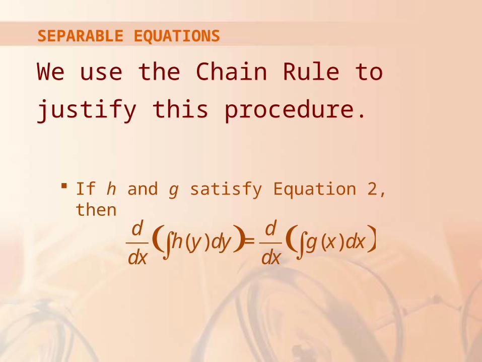
We use the Chain Rule to justify this

procedure.

If h and g satisfy Equation 2, then

( ) ( )( ) ( )d d

h y dy g x dxdx dx

=∫ ∫

SEPARABLE EQUATIONS

Thus,

This gives:

Thus, Equation 1 is satisfied.

( )( ) ( )d dy

h y dy g xdy dx

=∫

( ) ( )dy

h y g xdx

=

SEPARABLE EQUATIONS

a.Solve the differential equation

b.Find the solution of this equation that

satisfies the initial condition y(0) = 2.

2

2

dy x

dx y=

SEPARABLE EQUATIONS Example 1

We write the equation in terms of differentials

and integrate both sides:

y2 dy = x2 dx

∫ y2 dy = ∫ x2 dx

⅓y3 = ⅓x3 + C

where C is an arbitrary constant.

SEPARABLE EQUATIONS Example 1 a

We could have used a constant C1 on

the left side and another constant C2 on

the right side.

However, then, we could combine these constants by writing C = C2 – C1.


Solving for y, we get:

We could leave the solution like this or we could write it in the form

where K = 3C. Since C is an arbitrary constant, so is K.

3 3 3y x C= +

3 3y x K= +


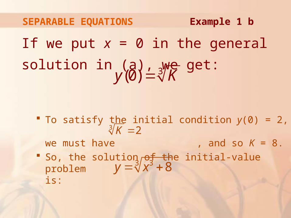
If we put x = 0 in the general solution in (a),

we get:

To satisfy the initial condition y(0) = 2, we must have , and so K = 8.

So, the solution of the initial-value problem is:

3(0)y K=

3 2K =

SEPARABLE EQUATIONS Example 1 b

3 3 8y x= +

The figure shows graphs of several members

of the family of solutions of the differential

equation in Example 1.

The solution of the initial-value problem in (b) is shown in red.

SEPARABLE EQUATIONS

Solve the differential equation

26

2 cos

dy x

dx y y=

+


Writing the equation in differential form

and integrating both sides, we have:

(2y + cos y) dy = 6x2 dx

∫ (2y + cos y) dy = ∫ 6x2 dx

y2 + sin y = 2x3 + C

where C is a constant.

SEPARABLE EQUATIONS E. g. 2—Equation 3

Equation 3 gives the general solution

implicitly.

In this case, it’s impossible to solve the equation to express y explicitly as a function of x.


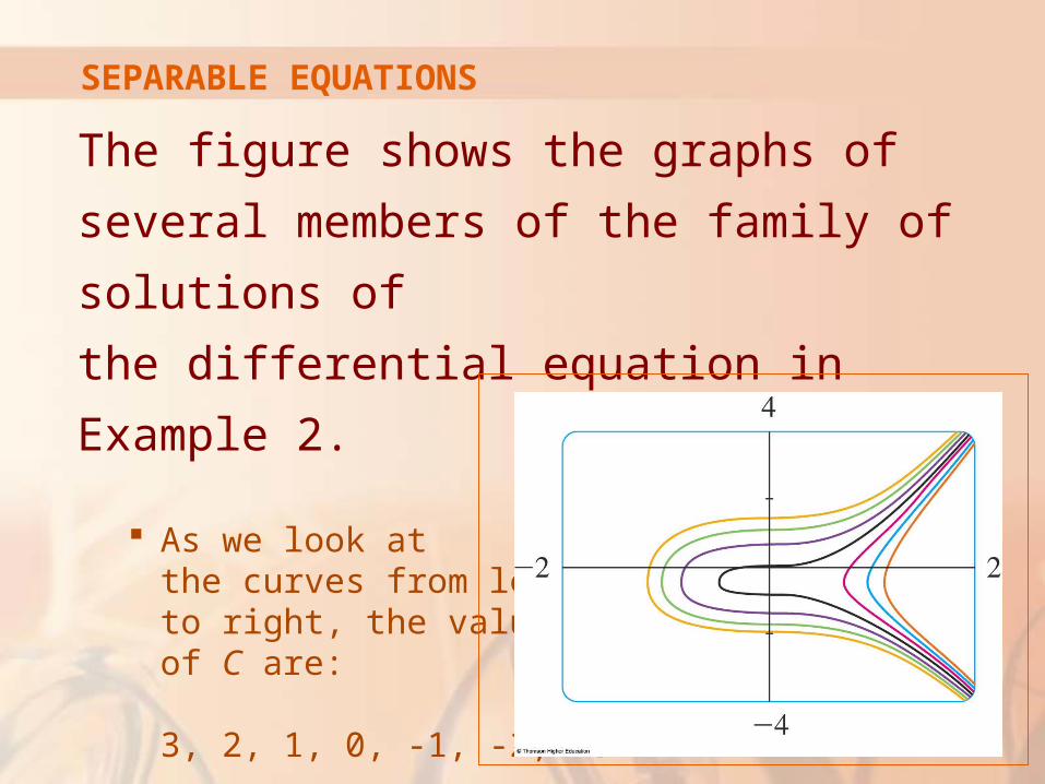
The figure shows the graphs of several

members of the family of solutions of

the differential equation in Example 2.

As we look at the curves from left to right, the values of C are:

3, 2, 1, 0, -1, -2, -3

SEPARABLE EQUATIONS

Solve the equation

y’ = x2y

First, we rewrite the equation using Leibniz notation:

2dyx y

dx=


If y ≠ 0, we can rewrite it in differential

notation and integrate:

2

2

3

0

ln3

dyx dx y

y

dyx dx

y

xy C

= ≠

=

= +

∫ ∫


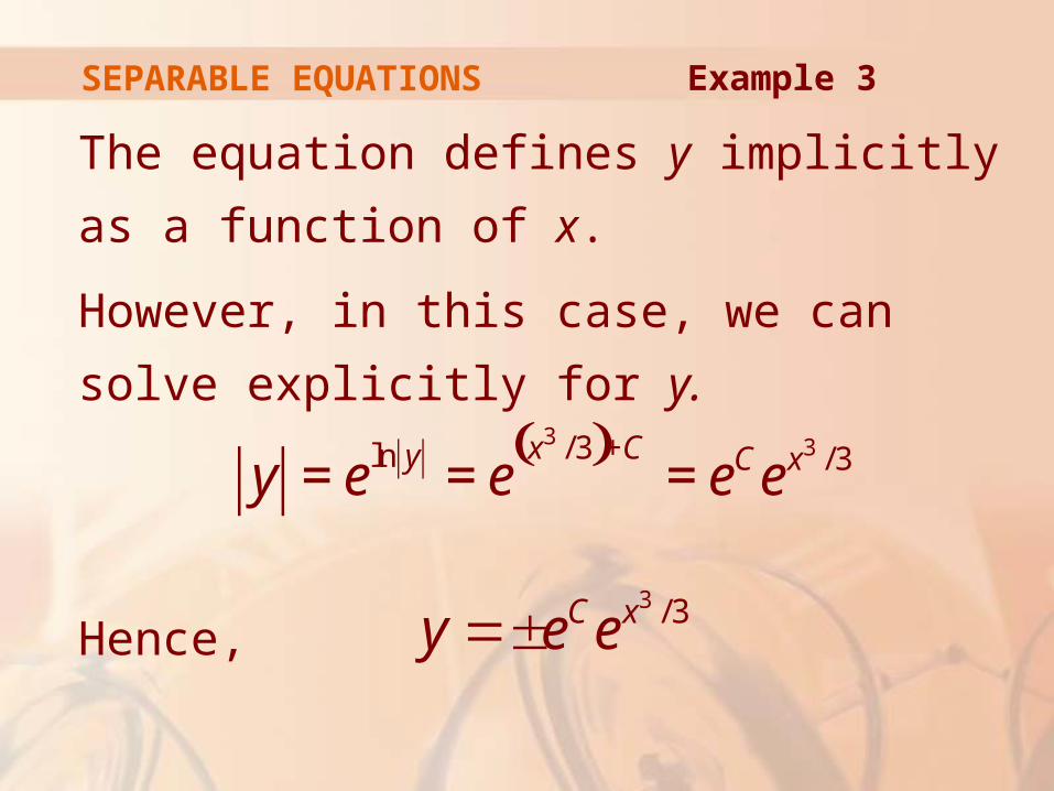
The equation defines y implicitly as a function

of x.

However, in this case, we can solve explicitly

for y.

Hence,

( )3 3/ 3ln /3x Cy C xy e e e e+

= = =


3 / 3C xy e e=±

We can easily verify that the function y = 0

is also a solution of the given differential

equation.

So, we can write the general solution in the form

where A is an arbitrary constant (A = eC, or A = –eC, or A = 0).

3 / 3xy Ae=


The figure shows a direction field for

the differential equation in Example 3.

Compare it with the next figure, in which we use the equation to graph solutions for several values of A.

3 / 3xy Ae=

SEPARABLE EQUATIONS

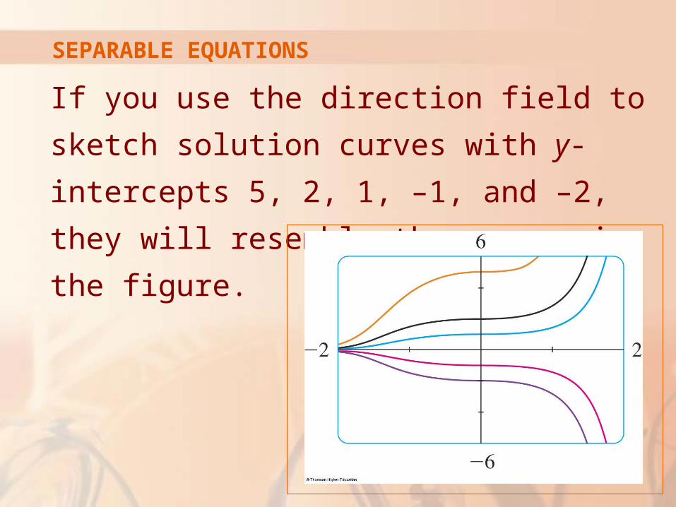
If you use the direction field to sketch solution

curves with y-intercepts 5, 2, 1, –1, and –2,

they will resemble the curves in the figure.

SEPARABLE EQUATIONS

In Section 9.2, we modeled the current I(t)

in this electric circuit by the differential

equation

( )dIL RI E tdt

+ =

Example 4SEPARABLE EQUATIONS

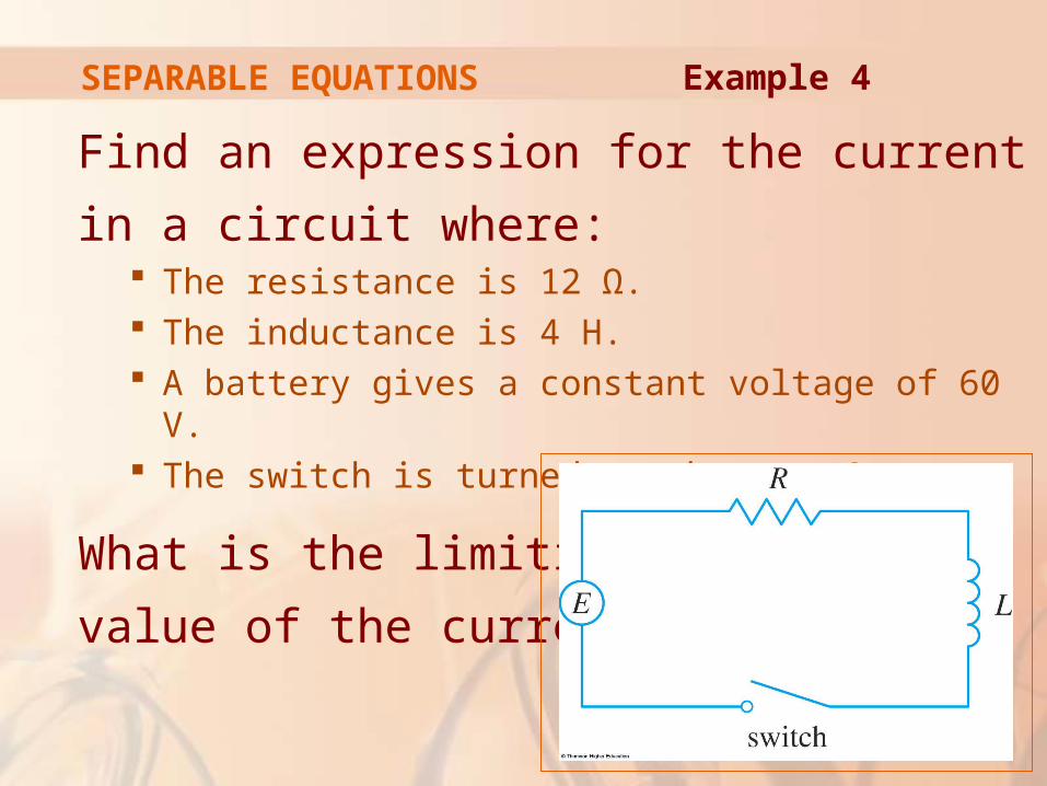
Find an expression for the current in a circuit

where: The resistance is 12 Ω. The inductance is 4 H. A battery gives a constant voltage of 60 V. The switch is turned on when t = 0.

What is the limiting

value of the current?


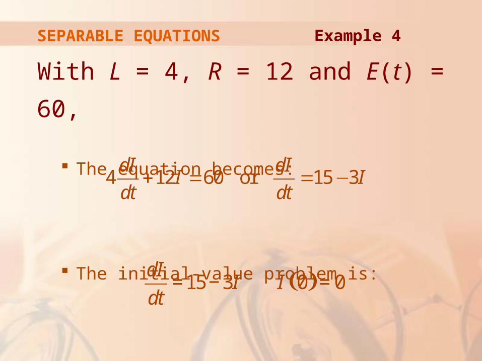
With L = 4, R = 12 and E(t) = 60,

The equation becomes:

The initial-value problem is:

4 12 60 or 15 3dI dI

I Idt dt

+ = = −


( )15 3 0 0dI

I Idt

= − =

We recognize this as being separable.

We solve it as follows:

( )

13

3

3 3 3

313

(15 3 0)15 3

ln 15 3

15 3

15 3

5

t C

C t t

t

dIdt I

II t C

I e

I e e Ae

I Ae

− +

− − −

−

= − ≠−

− − = +

− =

− = ± =

= −

∫ ∫


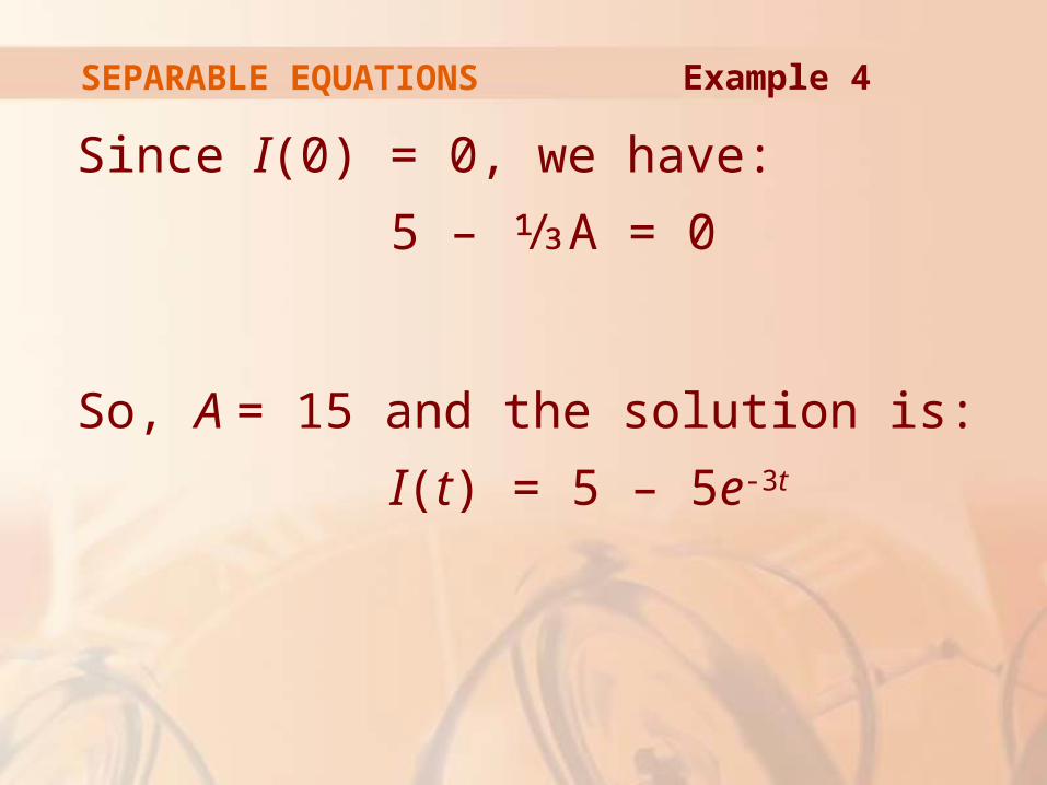
Since I(0) = 0, we have:

5 – ⅓A = 0

So, A = 15 and the solution is:

I(t) = 5 – 5e-3t



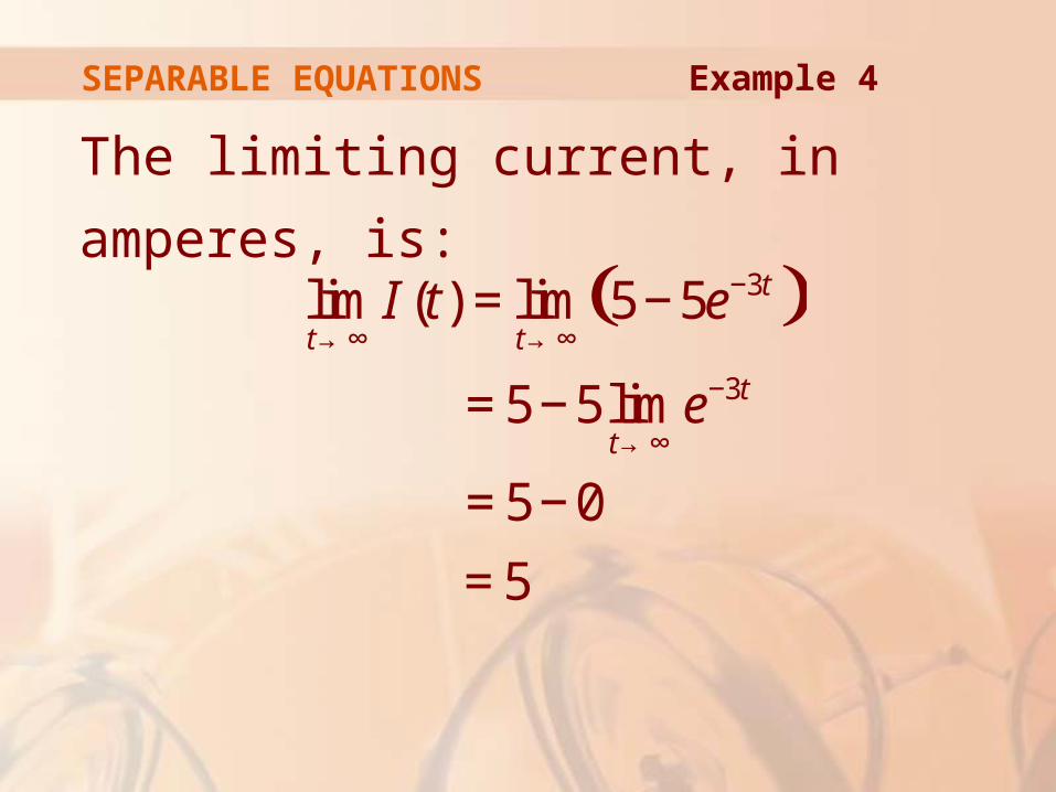
The limiting current, in amperes, is:

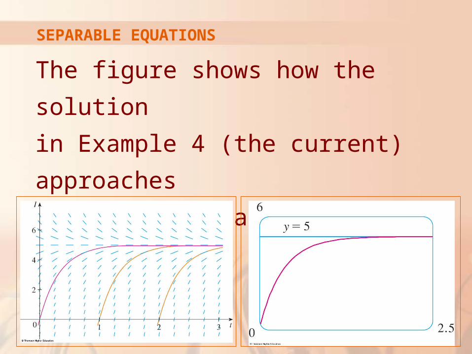
The figure shows how the solution

in Example 4 (the current) approaches

its limiting value.

SEPARABLE EQUATIONS

Comparison with the other figure (from

Section 9.2) shows that we were able to

draw a fairly accurate solution curve from

the direction field.

SEPARABLE EQUATIONS

An orthogonal trajectory of a family of curves

is a curve that intersects each curve of the

family orthogonally—that is, at right angles.

ORTHOGONAL TRAJECTORY

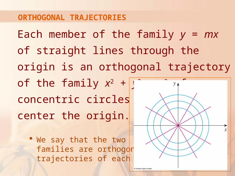
Each member of the family y = mx of straight

lines through the origin is an orthogonal

trajectory of the family x2 + y2 = r2 of concentric

circles with

center the origin.

We say that the two families are orthogonal trajectories of each other.

ORTHOGONAL TRAJECTORIES

Find the orthogonal trajectories of

the family of curves x = ky2, where k

is an arbitrary constant.

ORTHOGONAL TRAJECTORIES Example 5

The curves x = ky2 form a family

of parabolas whose axis of symmetry

is the x-axis.

The first step is to find a single differential equation that is satisfied by all members of the family.


If we differentiate x = ky2, we get:

This differential equation depends on k. However, we need an equation that is valid

for all values of k simultaneously.

11 2 or =

2

dy dykydx dx ky

=


To eliminate k, we note that:

From the equation of the given general parabola x = ky2, we have k = x/y2.


Hence, the differential equation can be

written as:

or

This means that the slope of the tangent line at any point (x, y) on one of the parabolas is: y’ = y/(2x)

2

1 1

2 2

dyxdx ky yy

= =


2

dy y

dx x=

On an orthogonal trajectory, the slope

of the tangent line must be the negative

reciprocal of this slope.

So, the orthogonal trajectories must satisfy the differential equation 2dy x

dx y=−

ORTHOGONAL TRAJECTORIES

The differential equation is separable.

We solve it as follows:

where C is an arbitrary positive constant.

22

22

2

2

2

y dy x dx

yx C

yx C

=−

=− +

+ =

∫ ∫

ORTHOGONAL TRAJECTORIES E. g. 5—Equation 4

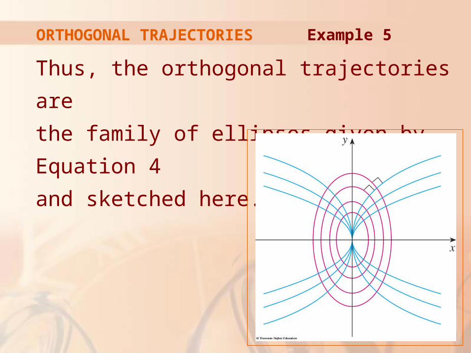
Thus, the orthogonal trajectories are

the family of ellipses given by Equation 4

and sketched here.


Orthogonal trajectories occur in various

branches of physics.

In an electrostatic field, the lines of force are orthogonal to the lines of constant potential.

The streamlines in aerodynamics are orthogonal trajectories of the velocity-equipotential curves.

ORTHOGONAL TRAJECTORIES IN PHYSICS

MIXING PROBLEMS

A typical mixing problem involves a tank

of fixed capacity filled with a thoroughly mixed

solution of some substance, such as salt.

A solution of a given concentration enters the tank at a fixed rate.

The mixture, thoroughly stirred, leaves at a fixed rate, which may differ from the entering rate.

If y(t) denotes the amount of substance in

the tank at time t, then y’(t) is the rate at which

the substance is being added minus the rate

at which it is being removed.

The mathematical description of this situation often leads to a first-order separable differential equation.

MIXING PROBLEMS

We can use the same type of reasoning

to model a variety of phenomena:

Chemical reactions

Discharge of pollutants into a lake

Injection of a drug into the bloodstream

MIXING PROBLEMS

A tank contains 20 kg of salt dissolved

in 5000 L of water.

Brine that contains 0.03 kg of salt per liter of water enters the tank at a rate of 25 L/min.

The solution is kept thoroughly mixed and drains from the tank at the same rate.

How much salt remains in the tank after half an hour?

MIXING PROBLEMS Example 6

Let y(t) be the amount of salt (in kilograms)

after t minutes.

We are given that y(0) = 20 and we want to

find y(30).

We do this by finding a differential equation satisfied by y(t).


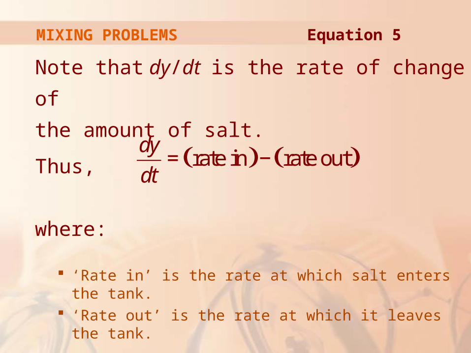
Note that dy/dt is the rate of change of

the amount of salt.

Thus,

where:

‘Rate in’ is the rate at which salt enters the tank. ‘Rate out’ is the rate at which it leaves the tank.

( ) ( )rate in rate outdy

dt= −

MIXING PROBLEMS Equation 5

We have:

kg Lrate in 0.03 25

L min

kg0.75

min

⎛ ⎞⎛ ⎞=⎜ ⎟⎜ ⎟⎝ ⎠⎝ ⎠

=

RATE IN Example 6

The tank always contains 5000 L

of liquid.

So, the concentration at time t is y(t)/5000 (measured in kg/L).


As the brine flows out at a rate of 25 L/min,

we have:

( ) kg Lrate out 25

5000 L min

( ) kg

200 min

y t

y t

⎛ ⎞⎛ ⎞=⎜ ⎟⎜ ⎟⎝ ⎠⎝ ⎠

=

RATE OUT Example 6

Thus, from Equation 5, we get:

Solving this separable differential equation, we obtain:

( ) 150 ( )0.75

200 200

dy y t y t

dt

−= − =

150 200

ln 150200

dy dt

y

ty C

=−

− − = +

∫ ∫


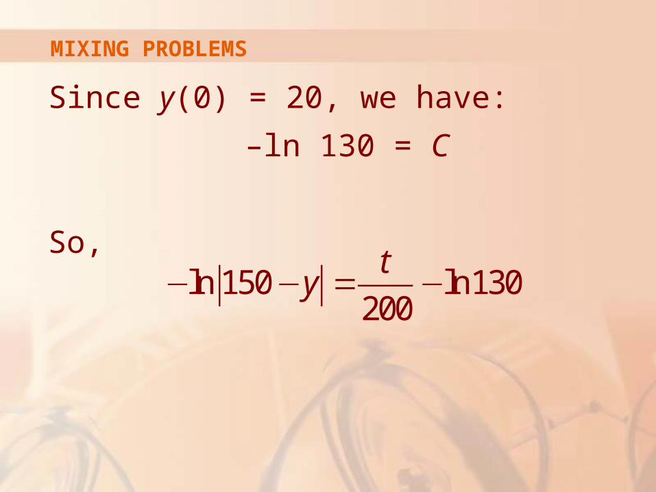
Since y(0) = 20, we have:

–ln 130 = C

So,ln 150 ln130

200

ty− − = −

MIXING PROBLEMS

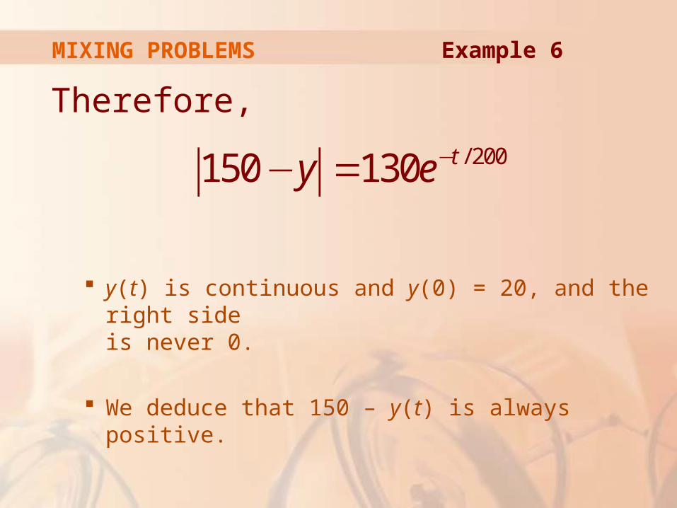
Therefore,

y(t) is continuous and y(0) = 20, and the right side is never 0.

We deduce that 150 – y(t) is always positive.

/ 200150 130 ty e−− =


Thus, |150 – y| = 150 – y.

So,

The amount of salt after 30 min is:

30 200(30) 150 130 38.1 kgy e−= − ≈


/ 200( ) 150 130 ty t e−= −

Here’s the graph of the function y(t)

of Example 6.

Notice that, as time goes by, the amount of salt approaches 150 kg.


differential equations 9. we have looked at first-order differential equations from a geometric...

Documents