differential equationsmachas/differential...preface what follows are my lecture notes for a first...
TRANSCRIPT

Differential Equations
Jeffrey R. Chasnov
Adapted for :Differential Equations for Engineers
Click to view a promotional video

The Hong Kong University of Science and TechnologyDepartment of MathematicsClear Water Bay, Kowloon
Hong Kong
Copyright c○ 2009–2019 by Jeffrey Robert Chasnov
This work is licensed under the Creative Commons Attribution 3.0 Hong Kong License. Toview a copy of this license, visit http://creativecommons.org/licenses/by/3.0/hk/ or senda letter to Creative Commons, 171 Second Street, Suite 300, San Francisco, California, 94105,USA.

PrefaceWhat follows are my lecture notes for a first course in differential equations, taughtat the Hong Kong University of Science and Technology. Included in these notesare links to short tutorial videos posted on YouTube.
Much of the material of Chapters 2-6 and 8 has been adapted from the widelyused textbook “Elementary differential equations and boundary value problems”by Boyce & DiPrima (John Wiley & Sons, Inc., Seventh Edition, c○2001). Many ofthe examples presented in these notes may be found in this book. The material ofChapter 7 is adapted from the textbook “Nonlinear dynamics and chaos” by StevenH. Strogatz (Perseus Publishing, c○1994).
All web surfers are welcome to download these notes, watch the YouTube videos,and to use the notes and videos freely for teaching and learning.
I also have some online courses on Coursera. A lot of time and effort has goneinto their production, and the video lectures have better video quality than the onesprepared for these notes. You can click on the links below to explore these courses.
If you want to learn differential equations, have a look at
Differential Equations for Engineers
If your interests are matrices and elementary linear algebra, try
Matrix Algebra for Engineers
If you want to learn vector calculus (also known as multivariable calculus, or calcu-lus three), you can sign up for
Vector Calculus for Engineers
And if your interest is numerical methods, have a go at
Numerical Methods for Engineers
Jeffrey R. Chasnov
Hong KongFebruary 2021
iii


Contents0 A short mathematical review 1
0.1 The trigonometric functions . . . . . . . . . . . . . . . . . . . . . . . . . 10.2 The exponential function and the natural logarithm . . . . . . . . . . . 10.3 Definition of the derivative . . . . . . . . . . . . . . . . . . . . . . . . . 20.4 Differentiating a combination of functions . . . . . . . . . . . . . . . . 2
0.4.1 The sum or difference rule . . . . . . . . . . . . . . . . . . . . . 20.4.2 The product rule . . . . . . . . . . . . . . . . . . . . . . . . . . . 20.4.3 The quotient rule . . . . . . . . . . . . . . . . . . . . . . . . . . . 20.4.4 The chain rule . . . . . . . . . . . . . . . . . . . . . . . . . . . . . 2
0.5 Differentiating elementary functions . . . . . . . . . . . . . . . . . . . . 30.5.1 The power rule . . . . . . . . . . . . . . . . . . . . . . . . . . . . 30.5.2 Trigonometric functions . . . . . . . . . . . . . . . . . . . . . . . 30.5.3 Exponential and natural logarithm functions . . . . . . . . . . . 3
0.6 Definition of the integral . . . . . . . . . . . . . . . . . . . . . . . . . . . 30.7 The fundamental theorem of calculus . . . . . . . . . . . . . . . . . . . 40.8 Definite and indefinite integrals . . . . . . . . . . . . . . . . . . . . . . . 50.9 Indefinite integrals of elementary functions . . . . . . . . . . . . . . . . 50.10 Substitution . . . . . . . . . . . . . . . . . . . . . . . . . . . . . . . . . . 60.11 Integration by parts . . . . . . . . . . . . . . . . . . . . . . . . . . . . . . 60.12 Taylor series . . . . . . . . . . . . . . . . . . . . . . . . . . . . . . . . . . 60.13 Functions of several variables . . . . . . . . . . . . . . . . . . . . . . . . 70.14 Complex numbers . . . . . . . . . . . . . . . . . . . . . . . . . . . . . . 8
1 Introduction to odes 131.1 The simplest type of differential equation . . . . . . . . . . . . . . . . . 13
2 First-order odes 152.1 The Euler method . . . . . . . . . . . . . . . . . . . . . . . . . . . . . . . 152.2 Separable equations . . . . . . . . . . . . . . . . . . . . . . . . . . . . . 162.3 Linear equations . . . . . . . . . . . . . . . . . . . . . . . . . . . . . . . 192.4 Applications . . . . . . . . . . . . . . . . . . . . . . . . . . . . . . . . . . 22
2.4.1 Compound interest . . . . . . . . . . . . . . . . . . . . . . . . . . 222.4.2 Chemical reactions . . . . . . . . . . . . . . . . . . . . . . . . . . 232.4.3 Terminal velocity . . . . . . . . . . . . . . . . . . . . . . . . . . . 252.4.4 Escape velocity . . . . . . . . . . . . . . . . . . . . . . . . . . . . 262.4.5 RC circuit . . . . . . . . . . . . . . . . . . . . . . . . . . . . . . . 272.4.6 The logistic equation . . . . . . . . . . . . . . . . . . . . . . . . . 29
3 Second-order odes, constant coefficients 313.1 The Euler method . . . . . . . . . . . . . . . . . . . . . . . . . . . . . . . 313.2 The principle of superposition . . . . . . . . . . . . . . . . . . . . . . . 323.3 The Wronskian . . . . . . . . . . . . . . . . . . . . . . . . . . . . . . . . 323.4 Homogeneous odes . . . . . . . . . . . . . . . . . . . . . . . . . . . . . . 33
3.4.1 Distinct real roots . . . . . . . . . . . . . . . . . . . . . . . . . . . 34
v
CONTENTS
3.4.2 Distinct complex-conjugate roots . . . . . . . . . . . . . . . . . . 363.4.3 Repeated roots . . . . . . . . . . . . . . . . . . . . . . . . . . . . 37
3.5 Inhomogeneous odes . . . . . . . . . . . . . . . . . . . . . . . . . . . . . 393.6 Inhomogeneous linear first-order odes revisited . . . . . . . . . . . . . 423.7 Resonance . . . . . . . . . . . . . . . . . . . . . . . . . . . . . . . . . . . 433.8 Applications . . . . . . . . . . . . . . . . . . . . . . . . . . . . . . . . . . 46
3.8.1 RLC circuit . . . . . . . . . . . . . . . . . . . . . . . . . . . . . . 463.8.2 Mass on a spring . . . . . . . . . . . . . . . . . . . . . . . . . . . 483.8.3 Pendulum . . . . . . . . . . . . . . . . . . . . . . . . . . . . . . . 49
3.9 Damped resonance . . . . . . . . . . . . . . . . . . . . . . . . . . . . . . 50
4 The Laplace transform 534.1 Definition and properties . . . . . . . . . . . . . . . . . . . . . . . . . . 534.2 Solution of initial value problems . . . . . . . . . . . . . . . . . . . . . . 574.3 Heaviside and Dirac delta functions . . . . . . . . . . . . . . . . . . . . 59
4.3.1 Heaviside function . . . . . . . . . . . . . . . . . . . . . . . . . . 604.3.2 Dirac delta function . . . . . . . . . . . . . . . . . . . . . . . . . 62
4.4 Discontinuous or impulsive terms . . . . . . . . . . . . . . . . . . . . . 63
5 Series solutions 675.1 Ordinary points . . . . . . . . . . . . . . . . . . . . . . . . . . . . . . . . 675.2 Regular singular points: Cauchy-Euler equations . . . . . . . . . . . . 70
5.2.1 Distinct real roots . . . . . . . . . . . . . . . . . . . . . . . . . . . 725.2.2 Distinct complex-conjugate roots . . . . . . . . . . . . . . . . . . 735.2.3 Repeated roots . . . . . . . . . . . . . . . . . . . . . . . . . . . . 73
6 Systems of equations 756.1 Matrices, determinants and the eigenvalue problem . . . . . . . . . . . 756.2 Coupled first-order equations . . . . . . . . . . . . . . . . . . . . . . . . 78
6.2.1 Distinct real eigenvalues . . . . . . . . . . . . . . . . . . . . . . . 786.2.2 Distinct complex-conjugate eigenvalues . . . . . . . . . . . . . . 826.2.3 Repeated eigenvalues with one eigenvector . . . . . . . . . . . 83
6.3 Normal modes . . . . . . . . . . . . . . . . . . . . . . . . . . . . . . . . . 86
7 Nonlinear differential equations 897.1 Fixed points and stability . . . . . . . . . . . . . . . . . . . . . . . . . . 89
7.1.1 One dimension . . . . . . . . . . . . . . . . . . . . . . . . . . . . 897.1.2 Two dimensions . . . . . . . . . . . . . . . . . . . . . . . . . . . 90
7.2 One-dimensional bifurcations . . . . . . . . . . . . . . . . . . . . . . . . 937.2.1 Saddle-node bifurcation . . . . . . . . . . . . . . . . . . . . . . . 937.2.2 Transcritical bifurcation . . . . . . . . . . . . . . . . . . . . . . . 947.2.3 Supercritical pitchfork bifurcation . . . . . . . . . . . . . . . . . 957.2.4 Subcritical pitchfork bifurcation . . . . . . . . . . . . . . . . . . 967.2.5 Application: a mathematical model of a fishery . . . . . . . . . 98
7.3 Two-dimensional bifurcations . . . . . . . . . . . . . . . . . . . . . . . . 997.3.1 Supercritical Hopf bifurcation . . . . . . . . . . . . . . . . . . . 1007.3.2 Subcritical Hopf bifurcation . . . . . . . . . . . . . . . . . . . . . 101
vi CONTENTS

CONTENTS
8 Partial differential equations 1038.1 Derivation of the diffusion equation . . . . . . . . . . . . . . . . . . . . 1038.2 Derivation of the wave equation . . . . . . . . . . . . . . . . . . . . . . 1048.3 Fourier series . . . . . . . . . . . . . . . . . . . . . . . . . . . . . . . . . 1058.4 Fourier sine and cosine series . . . . . . . . . . . . . . . . . . . . . . . . 1078.5 Solution of the diffusion equation . . . . . . . . . . . . . . . . . . . . . 110
8.5.1 Homogeneous boundary conditions . . . . . . . . . . . . . . . . 1108.5.2 Inhomogeneous boundary conditions . . . . . . . . . . . . . . . 1148.5.3 Pipe with closed ends . . . . . . . . . . . . . . . . . . . . . . . . 115
8.6 Solution of the wave equation . . . . . . . . . . . . . . . . . . . . . . . . 1178.6.1 Plucked string . . . . . . . . . . . . . . . . . . . . . . . . . . . . . 1178.6.2 Hammered string . . . . . . . . . . . . . . . . . . . . . . . . . . . 1198.6.3 General initial conditions . . . . . . . . . . . . . . . . . . . . . . 119
8.7 The Laplace equation . . . . . . . . . . . . . . . . . . . . . . . . . . . . . 1208.7.1 Dirichlet problem for a rectangle . . . . . . . . . . . . . . . . . . 1208.7.2 Dirichlet problem for a circle . . . . . . . . . . . . . . . . . . . . 122
8.8 The Schrödinger equation . . . . . . . . . . . . . . . . . . . . . . . . . . 1258.8.1 Heuristic derivation of the Schrödinger equation . . . . . . . . 1258.8.2 The time-independent Schrödinger equation . . . . . . . . . . . 1278.8.3 Particle in a one-dimensional box . . . . . . . . . . . . . . . . . 1278.8.4 The simple harmonic oscillator . . . . . . . . . . . . . . . . . . . 1288.8.5 Particle in a three-dimensional box . . . . . . . . . . . . . . . . 1318.8.6 The hydrogen atom . . . . . . . . . . . . . . . . . . . . . . . . . 132
CONTENTS vii

CONTENTS
viii CONTENTS

Chapter 0
A short mathematical reviewA basic understanding of calculus is required to undertake a study of differential
equations. This zero chapter presents a short review.
0.1 The trigonometric functions
The Pythagorean trigonometric identity is
sin2 x + cos2 x = 1,
and the addition theorems are
sin(x + y) = sin(x) cos(y) + cos(x) sin(y),cos(x + y) = cos(x) cos(y)− sin(x) sin(y).
Also, the values of sin x in the first quadrant can be remembered by the rule ofquarters, with 0∘ = 0, 30∘ = π/6, 45∘ = π/4, 60∘ = π/3, 90∘ = π/2:
sin 0∘ =
√04
, sin 30∘ =
√14
, sin 45∘ =
√24
,
sin 60∘ =
√34
, sin 90∘ =
√44
.
The following symmetry properties are also useful:
sin(π/2 − x) = cos x, cos(π/2 − x) = sin x;
andsin(−x) = − sin(x), cos(−x) = cos(x).
0.2 The exponential function and the natural logarithm
The transcendental number e, approximately 2.71828, is defined as
e = limn→∞
(1 +
1n
)n.
The exponential function exp (x) = ex and natural logarithm ln x are inverse func-tions satisfying
eln x = x, ln ex = x.
The usual rules of exponents apply:
exey = ex+y, ex/ey = ex−y, (ex)p = epx.
The corresponding rules for the logarithmic function are
ln (xy) = ln x + ln y, ln (x/y) = ln x − ln y, ln xp = p ln x.
1

0.3. DEFINITION OF THE DERIVATIVE
0.3 Definition of the derivative
The derivative of the function y = f (x), denoted as f ′(x) or dy/dx, is defined asthe slope of the tangent line to the curve y = f (x) at the point (x, y). This slope isobtained by a limit, and is defined as
f ′(x) = limh→0
f (x + h)− f (x)h
. (1)
0.4 Differentiating a combination of functions
0.4.1 The sum or difference rule
The derivative of the sum of f (x) and g(x) is
( f + g)′ = f ′ + g′.
Similarly, the derivative of the difference is
( f − g)′ = f ′ − g′.
0.4.2 The product rule
The derivative of the product of f (x) and g(x) is
( f g)′ = f ′g + f g′,
and should be memorized as “the derivative of the first times the second plus thefirst times the derivative of the second.”
0.4.3 The quotient rule
The derivative of the quotient of f (x) and g(x) is(fg
)′=
f ′g − f g′
g2 ,
and should be memorized as “the derivative of the top times the bottom minus thetop times the derivative of the bottom over the bottom squared.”
0.4.4 The chain rule
The derivative of the composition of f (x) and g(x) is(f(
g(x)))′
= f ′(
g(x))· g′(x),
and should be memorized as “the derivative of the outside times the derivative ofthe inside.”
2 CHAPTER 0. A SHORT MATHEMATICAL REVIEW

0.5. DIFFERENTIATING ELEMENTARY FUNCTIONS
0.5 Differentiating elementary functions
0.5.1 The power ruleThe derivative of a power of x is given by
ddx
xp = pxp−1.
0.5.2 Trigonometric functionsThe derivatives of sin x and cos x are
(sin x)′ = cos x, (cos x)′ = − sin x.
We thus say that “the derivative of sine is cosine,” and “the derivative of cosine isminus sine.” Notice that the second derivatives satisfy
(sin x)′′ = − sin x, (cos x)′′ = − cos x.
0.5.3 Exponential and natural logarithm functionsThe derivative of ex and ln x are
(ex)′ = ex, (ln x)′ =1x
.
0.6 Definition of the integral
The definite integral of a function f (x) > 0 from x = a to b (b > a) is definedas the area bounded by the vertical lines x = a, x = b, the x-axis and the curvey = f (x). This “area under the curve” is obtained by a limit. First, the area isapproximated by a sum of rectangle areas. Second, the integral is defined to be thelimit of the rectangle areas as the width of each individual rectangle goes to zeroand the number of rectangles goes to infinity. This resulting infinite sum is called aRiemann Sum, and we define
∫ b
af (x)dx = lim
h→0
N
∑n=1
f(a + (n − 1)h
)· h, (2)
where N = (b − a)/h is the number of terms in the sum. The symbols on the left-hand-side of (2) are read as “the integral from a to b of f of x dee x.” The RiemannSum definition is extended to all values of a and b and for all values of f (x) (positiveand negative). Accordingly,∫ a
bf (x)dx = −
∫ b
af (x)dx and
∫ b
a(− f (x))dx = −
∫ b
af (x)dx.
Also, ∫ c
af (x)dx =
∫ b
af (x)dx +
∫ c
bf (x)dx,
which states when f (x) > 0 and a < b < c that the total area is equal to the sum ofits parts.
CHAPTER 0. A SHORT MATHEMATICAL REVIEW 3

0.7. THE FUNDAMENTAL THEOREM OF CALCULUS
0.7 The fundamental theorem of calculus
View tutorial on YouTube
Using the definition of the derivative, we differentiate the following integral:
ddx
∫ x
af (s)ds = lim
h→0
∫ x+ha f (s)ds −
∫ xa f (s)ds
h
= limh→0
∫ x+hx f (s)ds
h
= limh→0
h f (x)h
= f (x).
This result is called the fundamental theorem of calculus, and provides a connectionbetween differentiation and integration.
The fundamental theorem teaches us how to integrate functions. Let F(x) be afunction such that F′(x) = f (x). We say that F(x) is an antiderivative of f (x). Thenfrom the fundamental theorem and the fact that the derivative of a constant equalszero,
F(x) =∫ x
af (s)ds + c.
Now, F(a) = c and F(b) =∫ b
a f (s)ds + F(a). Therefore, the fundamental theoremshows us how to integrate a function f (x) provided we can find its antiderivative:
∫ b
af (s)ds = F(b)− F(a). (3)
Unfortunately, finding antiderivatives is much harder than finding derivatives, andindeed, most complicated functions cannot be integrated analytically.
We can also derive the very important result (3) directly from the definition ofthe derivative (1) and the definite integral (2). We will see it is convenient to choosethe same h in both limits. With F′(x) = f (x), we have
∫ b
af (s)ds =
∫ b
aF′(s)ds
= limh→0
N
∑n=1
F′(a + (n − 1)h)· h
= limh→0
N
∑n=1
F(a + nh)− F(a + (n − 1)h
)h
· h
= limh→0
N
∑n=1
F(a + nh)− F(a + (n − 1)h
).
The last expression has an interesting structure. All the values of F(x) evaluatedat the points lying between the endpoints a and b cancel each other in consecutiveterms. Only the value −F(a) survives when n = 1, and the value +F(b) whenn = N, yielding again (3).
4 CHAPTER 0. A SHORT MATHEMATICAL REVIEW

0.8. DEFINITE AND INDEFINITE INTEGRALS
0.8 Definite and indefinite integrals
The Riemann sum definition of an integral is called a definite integral. It is convenientto also define an indefinite integral by∫
f (x)dx = F(x),
where F(x) is the antiderivative of f (x).
0.9 Indefinite integrals of elementary functions
From our known derivatives of elementary functions, we can determine some sim-ple indefinite integrals. The power rule gives us∫
xndx =xn+1
n + 1+ c, n = −1.
When n = −1, and x is positive, we have∫ 1x
dx = ln x + c.
If x is negative, using the chain rule we have
ddx
ln (−x) =1x
.
Therefore, since
|x| ={
−x if x < 0;x if x > 0,
we can generalize our indefinite integral to strictly positive or strictly negative x:∫ 1x
dx = ln |x|+ c.
Trigonometric functions can also be integrated:∫cos xdx = sin x + c,
∫sin xdx = − cos x + c.
Easily proved identities are an addition rule:∫ (f (x) + g(x)
)dx =
∫f (x)dx +
∫g(x)dx;
and multiplication by a constant:∫A f (x)dx = A
∫f (x)dx.
This permits integration of functions such as∫(x2 + 7x + 2)dx =
x3
3+
7x2
2+ 2x + c,
and ∫(5 cos x + sin x)dx = 5 sin x − cos x + c.
CHAPTER 0. A SHORT MATHEMATICAL REVIEW 5

0.10. SUBSTITUTION
0.10 Substitution
More complicated functions can be integrated using the chain rule. Since
ddx
f(
g(x))= f ′
(g(x)
)· g′(x),
we have ∫f ′(
g(x))· g′(x)dx = f
(g(x)
)+ c.
This integration formula is usually implemented by letting y = g(x). Then onewrites dy = g′(x)dx to obtain∫
f ′(
g(x))
g′(x)dx =∫
f ′(y)dy
= f (y) + c
= f(
g(x))+ c.
0.11 Integration by parts
Another integration technique makes use of the product rule for differentiation.Since
( f g)′ = f ′g + f g′,
we havef ′g = ( f g)′ − f g′.
Therefore, ∫f ′(x)g(x)dx = f (x)g(x)−
∫f (x)g′(x)dx.
Commonly, the above integral is done by writing
u = g(x) dv = f ′(x)dxdu = g′(x)dx v = f (x).
Then, the formula to be memorized is∫udv = uv −
∫vdu.
0.12 Taylor series
A Taylor series of a function f (x) about a point x = a is a power series repre-sentation of f (x) developed so that all the derivatives of f (x) at a match all thederivatives of the power series. Without worrying about convergence here, we have
f (x) = f (a) + f ′(a)(x − a) +f ′′(a)
2!(x − a)2 +
f ′′′(a)3!
(x − a)3 + . . . .
Notice that the first term in the power series matches f (a), all other terms vanishing,the second term matches f ′(a), all other terms vanishing, etc. Commonly, the Taylor
6 CHAPTER 0. A SHORT MATHEMATICAL REVIEW
0.13. FUNCTIONS OF SEVERAL VARIABLES
series is developed with a = 0. We will also make use of the Taylor series in aslightly different form, with x = x* + ε and a = x*:
f (x* + ε) = f (x*) + f ′(x*)ε +f ′′(x*)
2!ε2 +
f ′′′(x*)3!
ε3 + . . . .
Another way to view this series is that of g(ε) = f (x* + ε), expanded about ε = 0.Taylor series that are commonly used include
ex = 1 + x +x2
2!+
x3
3!+ . . . ,
sin x = x − x3
3!+
x5
5!− . . . ,
cos x = 1 − x2
2!+
x4
4!− . . . ,
11 + x
= 1 − x + x2 − . . . , for |x| < 1,
ln (1 + x) = x − x2
2+
x3
3− . . . , for |x| < 1.
0.13 Functions of several variables
For simplicity, we consider a function f = f (x, y) of two variables, though theresults are easily generalized. The partial derivative of f with respect to x is definedas
∂ f∂x
= limh→0
f (x + h, y)− f (x, y)h
,
and similarly for the partial derivative of f with respect to y. To take the partialderivative of f with respect to x, say, take the derivative of f with respect to xholding y fixed. As an example, consider
f (x, y) = 2x3y2 + y3.
We have∂ f∂x
= 6x2y2,∂ f∂y
= 4x3y + 3y2.
Second derivatives are defined as the derivatives of the first derivatives, so we have
∂2 f∂x2 = 12xy2,
∂2 f∂y2 = 4x3 + 6y;
and the mixed second partial derivatives are
∂2 f∂x∂y
= 12x2y,∂2 f
∂y∂x= 12x2y.
In general, mixed partial derivatives are independent of the order in which thederivatives are taken.
Partial derivatives are necessary for applying the chain rule. Consider
d f = f (x + dx, y + dy)− f (x, y).
CHAPTER 0. A SHORT MATHEMATICAL REVIEW 7

0.14. COMPLEX NUMBERS
We can write d f as
d f = [ f (x + dx, y + dy)− f (x, y + dy)] + [ f (x, y + dy)− f (x, y)]
=∂ f∂x
dx +∂ f∂y
dy.
If one has f = f (x(t), y(t)), say, then
d fdt
=∂ f∂x
dxdt
+∂ f∂y
dydt
.
And if one has f = f (x(r, θ), y(r, θ)), say, then
∂ f∂r
=∂ f∂x
∂x∂r
+∂ f∂y
∂y∂r
,∂ f∂θ
=∂ f∂x
∂x∂θ
+∂ f∂y
∂y∂θ
.
A Taylor series of a function of several variables can also be developed. Here, allpartial derivatives of f (x, y) at (a, b) match all the partial derivatives of the powerseries. With the notation
fx =∂ f∂x
, fy =∂ f∂y
, fxx =∂2 f∂x2 , fxy =
∂2 f∂x∂y
, fyy =∂2 f∂y2 , etc.,
we have
f (x, y) = f (a, b) + fx(a, b)(x − a) + fy(a, b)(y − b)
+12!
(fxx(a, b)(x − a)2 + 2 fxy(a, b)(x − a)(y − b) + fyy(a, b)(y − b)2
)+ . . .
0.14 Complex numbers
View tutorial on YouTube: Complex NumbersView tutorial on YouTube: Complex Exponential Function
We define the imaginary number i to be one of the two numbers that satisfies therule (i)2 = −1, the other number being −i. Formally, we write i =
√−1. A complex
number z is written asz = x + iy,
where x and y are real numbers. We call x the real part of z and y the imaginarypart and write
x = Re z, y = Im z.
Two complex numbers are equal if and only if their real and imaginary parts areequal.
The complex conjugate of z = x + iy, denoted as z, is defined as
z = x − iy.
Using z and z, we have
Re z =12(z + z) , Im z =
12i
(z − z) . (4)
8 CHAPTER 0. A SHORT MATHEMATICAL REVIEW

0.14. COMPLEX NUMBERS
Furthermore,
zz = (x + iy)(x − iy)
= x2 − i2y2
= x2 + y2;
and we define the absolute value of z, also called the modulus of z, by
|z| = (zz)1/2
=√
x2 + y2.
We can add, subtract, multiply and divide complex numbers to get new complexnumbers. With z = x + iy and w = s + it, and x, y, s, t real numbers, we have
z + w = (x + s) + i(y + t); z − w = (x − s) + i(y − t);
zw = (x + iy)(s + it)= (xs − yt) + i(xt + ys);
zw
=zwww
=(x + iy)(s − it)
s2 + t2
=(xs + yt)
s2 + t2 + i(ys − xt)
s2 + t2 .
Furthermore,
|zw| =√(xs − yt)2 + (xt + ys)2
=√(x2 + y2)(s2 + t2)
= |z||w|;and
zw = (xs − yt)− i(xt + ys)= (x − iy)(s − it)= zw.
Similarly ∣∣∣ zw
∣∣∣ = |z||w| , (
zw) =
zw
.
Also, z + w = z + w. However, |z + w| ≤ |z|+ |w|, a theorem known as the triangleinequality.
It is especially interesting and useful to consider the exponential function of animaginary argument. Using the Taylor series expansion of an exponential function,we have
eiθ = 1 + (iθ) +(iθ)2
2!+
(iθ)3
3!+
(iθ)4
4!+
(iθ)5
5!. . .
=
(1 − θ2
2!+
θ4
4!− . . .
)+ i(
θ − θ3
3!+
θ5
5!+ . . .
)= cos θ + i sin θ.
CHAPTER 0. A SHORT MATHEMATICAL REVIEW 9

0.14. COMPLEX NUMBERS
Since we have determined that
cos θ = Re eiθ , sin θ = Im eiθ , (5)
we also have using (4) and (5), the frequently used expressions
cos θ =eiθ + e−iθ
2, sin θ =
eiθ − e−iθ
2i.
The much celebrated Euler’s identity derives from eiθ = cos θ + i sin θ by settingθ = π, and using cos π = −1 and sin π = 0:
eiπ + 1 = 0,
and this identity links the five fundamental numbers—0, 1, i, e and π—using threebasic mathematical operations—addition, multiplication and exponentiation—onlyonce.
z=x+iy
θ
r
x
Re(z)
y
Im(z
)
Figure 1: The complex plane.
The complex number z can be represented in the complex plane with Re z as thex-axis and Im z as the y-axis (see Fig. 1). This leads to the polar representation ofz = x + iy:
z = reiθ ,
where r = |z| and tan θ = y/x. We define arg z = θ. Note that θ is not unique,though it is conventional to choose the value such that −π < θ ≤ π, and θ = 0when r = 0.
The polar form of a complex number can be useful when multiplying numbers.For example, if z1 = r1eiθ1 and z2 = r2eiθ2 , then z1z2 = r1r2ei(θ1+θ2). In particular, ifr2 = 1, then multiplication of z1 by z2 spins the representation of z1 in the complexplane an angle θ2 counterclockwise.
Useful trigonometric relations can be derived using eiθ and properties of theexponential function. The addition law can be derived from
ei(x+y) = eixeiy.
10 CHAPTER 0. A SHORT MATHEMATICAL REVIEW

0.14. COMPLEX NUMBERS
We have
cos(x + y) + i sin(x + y) = (cos x + i sin x)(cos y + i sin y)= (cos x cos y − sin x sin y) + i(sin x cos y + cos x sin y);
yielding
cos(x + y) = cos x cos y − sin x sin y, sin(x + y) = sin x cos y + cos x sin y.
De Moivre’s Theorem derives from einθ = (eiθ)n, yielding the identity
cos(nθ) + i sin(nθ) = (cos θ + i sin θ)n.
For example, if n = 2, we derive
cos 2θ + i sin 2θ = (cos θ + i sin θ)2
= (cos2 θ − sin2 θ) + 2i cos θ sin θ.
Therefore,cos 2θ = cos2 θ − sin2 θ, sin 2θ = 2 cos θ sin θ.
Example: Write√
i as a standard complex number
To solve this example, we first need to define what is meant by the square rootof a complex number. The meaning of
√z is the complex number whose square
is z. There will always be two such numbers, because (√
z)2 = (−√
z)2 = z. Onecan not define the positive square root because complex numbers are not definedas positive or negative.
We will show two methods to solve this problem. The first most straightforwardmethod writes √
i = x + iy.
Squaring both sides, we obtain
i = x2 − y2 + 2xyi;
and equating the real and imaginary parts of this equation yields the two real equa-tions
x2 − y2 = 0, 2xy = 1.
The first equation yields y = ±x. With y = x, the second equation yields 2x2 = 1with two solutions x = ±
√2/2. With y = −x, the second equation yields −2x2 = 1,
which has no solution for real x. We have therefore found that
√i = ±
(√2
2+ i
√2
2
).
The second solution method makes use of the polar form of complex numbers.The algebra required for this method is somewhat simpler, especially for findingcube roots, fourth roots, etc. We know that i = eiπ/2, but more generally because ofthe periodic nature of the polar angle, we can write
i = ei( π2 +2πk),
CHAPTER 0. A SHORT MATHEMATICAL REVIEW 11

0.14. COMPLEX NUMBERS
where k is an integer. We then have√
i = i1/2 = ei( π4 +πk) = eiπkeiπ/4 = ±eiπ/4,
where we have made use of the usual properties of the exponential function, andeiπk = ±1 for k even or odd. Converting back to standard form, we have
√i = ± (cos π/4 + i sin π/4) = ±
(√2
2+ i
√2
2
).
The fundamental theorem of algebra states that every polynomial equation ofdegree n has exactly n complex roots, counted with multiplicity. Two familiar ex-amples would be x2 − 1 = (x + 1)(x − 1) = 0, with two roots x1 = −1 and x2 = 1;and x2 − 2x + 1 = (x − 1)2 = 0, with one root x1 = 1 with multiplicity two.
The problem of finding the nth roots of unity is to solve the polynomial equation
zn = 1
for the n complex values of z. We have z1 = 1 for n = 1; and z1 = 1, z2 = −1 forn = 2. Beyond n = 2, some of the roots are complex and here we find the cuberoots of unity, that is, the three values of z that satisfy z3 = 1. Writing 1 = ei2πk,where k is an integer, we have
z = (1)1/3 =(
ei2πk)1/3
= ei2πk/3 =
1;ei2π/3;ei4π/3.
Using cos (2π/3) = −1/2, sin (2π/3) =√
3/2, cos (4π/3) = −1/2, sin (4π/3) =−√
3/2, the three cube roots of unity are given by
z1 = 1, z2 = −12+ i
√3
2, z3 = −1
2− i
√3
2.
These three roots are evenly spaced around the unit circle in the complex plane, asshown in the figure below.
ei2π/3
ei4π/3
1
12 CHAPTER 0. A SHORT MATHEMATICAL REVIEW

Chapter 1
Introduction to odesA differential equation is an equation for a function that relates the values of the
function to the values of its derivatives. An ordinary differential equation (ode) is adifferential equation for a function of a single variable, e.g., x(t), while a partial dif-ferential equation (pde) is a differential equation for a function of several variables,e.g., v(x, y, z, t). An ode contains ordinary derivatives and a pde contains partialderivatives. Typically, pde’s are much harder to solve than ode’s.
1.1 The simplest type of differential equation
View tutorial on YouTube
The simplest ordinary differential equations can be integrated directly by findingantiderivatives. These simplest odes have the form
dnxdtn = G(t),
where the derivative of x = x(t) can be of any order, and the right-hand-side maydepend only on the independent variable t. As an example, consider a mass fallingunder the influence of constant gravity, such as approximately found on the Earth’ssurface. Newton’s law, F = ma, results in the equation
md2xdt2 = −mg,
where x is the height of the object above the ground, m is the mass of the object, andg = 9.8 meter/sec2 is the constant gravitational acceleration. As Galileo suggested,the mass cancels from the equation, and
d2xdt2 = −g.
Here, the right-hand-side of the ode is a constant. The first integration, obtained byantidifferentiation, yields
dxdt
= A − gt,
with A the first constant of integration; and the second integration yields
x = B + At − 12
gt2,
with B the second constant of integration. The two constants of integration A andB can then be determined from the initial conditions. If we know that the initialheight of the mass is x0, and the initial velocity is v0, then the initial conditions are
x(0) = x0,dxdt
(0) = v0.
13

1.1. THE SIMPLEST TYPE OF DIFFERENTIAL EQUATION
Substitution of these initial conditions into the equations for dx/dt and x allows usto solve for A and B. The unique solution that satisfies both the ode and the initialconditions is given by
x(t) = x0 + v0t − 12
gt2. (1.1)
For example, suppose we drop a ball off the top of a 50 meter building. How longwill it take the ball to hit the ground? This question requires solution of (1.1) forthe time T it takes for x(T) = 0, given x0 = 50 meter and v0 = 0. Solving for T,
T =
√2x0
g
=
√2 · 509.8
sec
≈ 3.2sec.
14 CHAPTER 1. INTRODUCTION TO ODES

Chapter 2
First-order differentialequations
Reference: Boyce and DiPrima, Chapter 2
The general first-order differential equation for the function y = y(x) is written as
dydx
= f (x, y), (2.1)
where f (x, y) can be any function of the independent variable x and the dependentvariable y. We first show how to determine a numerical solution of this equa-tion, and then learn techniques for solving analytically some special forms of (2.1),namely, separable and linear first-order equations.
2.1 The Euler method
View tutorial on YouTube
Although it is not always possible to find an analytical solution of (2.1) for y =y(x), it is always possible to determine a unique numerical solution given an initialvalue y(x0) = y0, and provided f (x, y) is a well-behaved function. The differentialequation (2.1) gives us the slope f (x0, y0) of the tangent line to the solution curvey = y(x) at the point (x0, y0). With a small step size ∆x = x1 − x0, the initialcondition (x0, y0) can be marched forward to (x1, y1) along the tangent line usingEuler’s method (see Fig. 2.1)
y1 = y0 + ∆x f (x0, y0).
This solution (x1, y1) then becomes the new initial condition and is marched for-ward to (x2, y2) along a newly determined tangent line with slope given by f (x1, y1).For small enough ∆x, the numerical solution converges to the exact solution.
15

2.2. SEPARABLE EQUATIONS
x0
x1
y0
y1
y1 = y
0+∆x f(x
0,y
0)
slope = f(x0,y
0)
Figure 2.1: The differential equation dy/dx = f (x, y), y(x0) = y0, is integrated to x = x1using the Euler method y1 = y0 + ∆x f (x0, y0), with ∆x = x1 − x0.
2.2 Separable equations
View tutorial on YouTube
A first-order ode is separable if it can be written in the form
g(y)dydx
= f (x), y(x0) = y0, (2.2)
where the function g(y) is independent of x and f (x) is independent of y. Integra-tion from x0 to x results in∫ x
x0
g(y(x))y′(x)dx =∫ x
x0
f (x)dx.
The integral on the left can be transformed by substituting u = y(x), du = y′(x)dx,and changing the lower and upper limits of integration to y(x0) = y0 and y(x) = y.Therefore, ∫ y
y0
g(u)du =∫ x
x0
f (x)dx,
and since u is a dummy variable of integration, we can write this in the equivalentform ∫ y
y0
g(y)dy =∫ x
x0
f (x)dx. (2.3)
A simpler procedure that also yields (2.3) is to treat dy/dx in (2.2) like a fraction.Multiplying (2.2) by dx results in
g(y)dy = f (x)dx,
which is a separated equation with all the dependent variables on the left-side, andall the independent variables on the right-side. Equation (2.3) then results directlyupon integration.
16 CHAPTER 2. FIRST-ORDER ODES
2.2. SEPARABLE EQUATIONS
Example: Solve dydx + 1
2 y = 32 , with y(0) = 2.
We first manipulate the differential equation to the form
dydx
=12(3 − y), (2.4)
and then treat dy/dx as if it was a fraction to separate variables:
dy3 − y
=12
dx.
We integrate the right-side from the initial condition x = 0 to x and the left-sidefrom the initial condition y(0) = 2 to y. Accordingly,∫ y
2
dy3 − y
=12
∫ x
0dx. (2.5)
The integrals in (2.5) need to be done. Note that y(x) < 3 for finite x or the integralon the left-side diverges. Therefore, 3 − y > 0 and integration yields
− ln (3 − y)]y
2 =12
x]x
0 ,
ln (3 − y) = −12
x,
3 − y = e−12 x,
y = 3 − e−12 x.
Since this is our first nontrivial analytical solution, it is prudent to check our result.We do this by differentiating our solution:
dydx
=12
e−12 x
=12(3 − y);
and checking the initial conditions, y(0) = 3 − e0 = 2. Therefore, our solutionsatisfies both the original ode and the initial condition.
Example: Solve dydx + 1
2 y = 32 , with y(0) = 4.
This is the identical differential equation as before, but with different initial condi-tions. We will jump directly to the integration step:∫ y
4
dy3 − y
=12
∫ x
0dx.
Now y(x) > 3, so that y − 3 > 0 and integration yields
− ln (y − 3)]y
4 =12
x]x
0 ,
ln (y − 3) = −12
x,
y − 3 = e−12 x,
y = 3 + e−12 x.
CHAPTER 2. FIRST-ORDER ODES 17
2.2. SEPARABLE EQUATIONS
0 1 2 3 4 5 6 70
1
2
3
4
5
6
x
y
dy/dx + y/2 = 3/2
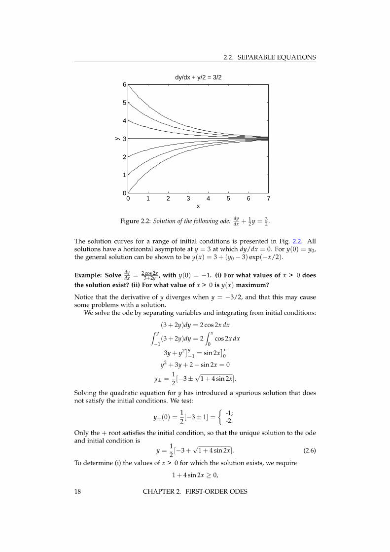
Figure 2.2: Solution of the following ode: dydx + 1
2 y = 32 .
The solution curves for a range of initial conditions is presented in Fig. 2.2. Allsolutions have a horizontal asymptote at y = 3 at which dy/dx = 0. For y(0) = y0,the general solution can be shown to be y(x) = 3 + (y0 − 3) exp(−x/2).
Example: Solve dydx = 2 cos 2x
3+2y , with y(0) = −1. (i) For what values of x > 0 doesthe solution exist? (ii) For what value of x > 0 is y(x) maximum?
Notice that the derivative of y diverges when y = −3/2, and that this may causesome problems with a solution.
We solve the ode by separating variables and integrating from initial conditions:
(3 + 2y)dy = 2 cos 2x dx∫ y
−1(3 + 2y)dy = 2
∫ x
0cos 2x dx
3y + y2]y−1 = sin 2x
]x0
y2 + 3y + 2 − sin 2x = 0
y± =12[−3 ±
√1 + 4 sin 2x].
Solving the quadratic equation for y has introduced a spurious solution that doesnot satisfy the initial conditions. We test:
y±(0) =12[−3 ± 1] =
{-1;-2.
Only the + root satisfies the initial condition, so that the unique solution to the odeand initial condition is
y =12[−3 +
√1 + 4 sin 2x]. (2.6)
To determine (i) the values of x > 0 for which the solution exists, we require
1 + 4 sin 2x ≥ 0,
18 CHAPTER 2. FIRST-ORDER ODES

2.3. LINEAR EQUATIONS
orsin 2x ≥ −1
4. (2.7)
Notice that at x = 0, we have sin 2x = 0; at x = π/4, we have sin 2x = 1; atx = π/2, we have sin 2x = 0; and at x = 3π/4, we have sin 2x = −1 We thereforeneed to determine the value of x such that sin 2x = −1/4, with x in the rangeπ/2 < x < 3π/4. The solution to the ode will then exist for all x between zero andthis value.
To solve sin 2x = −1/4 for x in the interval π/2 < x < 3π/4, one needs torecall the definition of arcsin, or sin−1, as found on a typical scientific calculator.The inverse of the function
f (x) = sin x, −π/2 ≤ x ≤ π/2
is denoted by arcsin. The first solution with x > 0 of the equation sin 2x = −1/4places 2x in the interval (π, 3π/2), so to invert this equation using the arcsinewe need to apply the identity sin (π − x) = sin x, and rewrite sin 2x = −1/4 assin (π − 2x) = −1/4. The solution of this equation may then be found by takingthe arcsine, and is
π − 2x = arcsin (−1/4),
or
x =12
(π + arcsin
14
).
Therefore the solution exists for 0 ≤ x ≤ (π + arcsin (1/4)) /2 = 1.6971 . . . , wherewe have used a calculator value (computing in radians) to find arcsin(0.25) =0.2527 . . . . At the value (x, y) = (1.6971 . . . ,−3/2), the solution curve ends anddy/dx becomes infinite.
To determine (ii) the value of x at which y = y(x) is maximum, we examine(2.6) directly. The value of y will be maximum when sin 2x takes its maximumvalue over the interval where the solution exists. This will be when 2x = π/2, orx = π/4 = 0.7854 . . . .
The graph of y = y(x) is shown in Fig. 2.3.
2.3 Linear equations
View tutorial on YouTube
The linear first-order differential equation (linear in y and its derivative) can bewritten in the form
dydx
+ p(x)y = g(x), (2.8)
with the initial condition y(x0) = y0. Linear first-order equations can be integratedusing an integrating factor µ(x). We multiply (2.8) by µ(x),
µ(x)[
dydx
+ p(x)y]= µ(x)g(x), (2.9)
and try to determine µ(x) so that
µ(x)[
dydx
+ p(x)y]=
ddx
[µ(x)y]. (2.10)
CHAPTER 2. FIRST-ORDER ODES 19

2.3. LINEAR EQUATIONS
0 0.5 1 1.5−1.6
−1.4
−1.2
−1
−0.8
−0.6
−0.4
−0.2
0
x
y
(3+2y) dy/dx = 2 cos 2x, y(0) = −1
Figure 2.3: Solution of the following ode: (3 + 2y)y′ = 2 cos 2x, y(0) = −1.
Equation (2.9) then becomes
ddx
[µ(x)y] = µ(x)g(x). (2.11)
Equation (2.11) is easily integrated using µ(x0) = µ0 and y(x0) = y0:
µ(x)y − µ0y0 =∫ x
x0
µ(x)g(x)dx,
or
y =1
µ(x)
(µ0y0 +
∫ x
x0
µ(x)g(x)dx)
. (2.12)
It remains to determine µ(x) from (2.10). Differentiating and expanding (2.10)yields
µdydx
+ pµy =dµ
dxy + µ
dydx
;
and upon simplifying,dµ
dx= pµ. (2.13)
Equation (2.13) is separable and can be integrated:∫ µ
µ0
dµ
µ=∫ x
x0
p(x)dx,
lnµ
µ0=∫ x
x0
p(x)dx,
µ(x) = µ0 exp(∫ x
x0
p(x)dx)
.
Notice that since µ0 cancels out of (2.12), it is customary to assign µ0 = 1. Thesolution to (2.8) satisfying the initial condition y(x0) = y0 is then commonly written
20 CHAPTER 2. FIRST-ORDER ODES

2.3. LINEAR EQUATIONS
as
y =1
µ(x)
(y0 +
∫ x
x0
µ(x)g(x)dx)
,
with
µ(x) = exp(∫ x
x0
p(x)dx)
the integrating factor. This important result finds frequent use in applied mathe-matics.
Example: Solve dydx + 2y = e−x, with y(0) = 3/4.
Note that this equation is not separable. With p(x) = 2 and g(x) = e−x, we have
µ(x) = exp(∫ x
02dx
)= e2x,
and
y = e−2x(
34+∫ x
0e2xe−xdx
)= e−2x
(34+∫ x
0exdx
)= e−2x
(34+ (ex − 1)
)= e−2x
(ex − 1
4
)= e−x
(1 − 1
4e−x)
.
Example: Solve dydx − 2xy = x, with y(0) = 0.
This equation is separable, and we solve it in two ways. First, using an integratingfactor with p(x) = −2x and g(x) = x:
µ(x) = exp(−2
∫ x
0xdx
)= e−x2
,
andy = ex2
∫ x
0xe−x2
dx.
The integral can be done by substitution with u = x2, du = 2xdx:
∫ x
0xe−x2
dx =12
∫ x2
0e−udu
= −12
e−u]x2
0
=12
(1 − e−x2
).
CHAPTER 2. FIRST-ORDER ODES 21

2.4. APPLICATIONS
Therefore,
y =12
ex2(
1 − e−x2)
=12
(ex2 − 1
).
Second, we integrate by separating variables:
dydx
− 2xy = x,
dydx
= x(1 + 2y),∫ y
0
dy1 + 2y
=∫ x
0xdx,
12
ln (1 + 2y) =12
x2,
1 + 2y = ex2,
y =12
(ex2 − 1
).
The results from the two different solution methods are the same, and the choice ofmethod is a personal preference.
2.4 Applications
2.4.1 Compound interestView tutorial on YouTube
The equation for the growth of an investment with continuous compounding ofinterest is a first-order differential equation. Let S(t) be the value of the investmentat time t, and let r be the annual interest rate compounded after every time interval∆t. We can also include deposits (or withdrawals). Let k be the annual depositamount, and suppose that an installment is deposited after every time interval ∆t.The value of the investment at the time t + ∆t is then given by
S(t + ∆t) = S(t) + (r∆t)S(t) + k∆t, (2.14)
where at the end of the time interval ∆t, r∆tS(t) is the amount of interest creditedand k∆t is the amount of money deposited (k > 0) or withdrawn (k < 0). As anumerical example, if the account held $10,000 at time t, and r = 6% per year andk = $12,000 per year, say, and the compounding and deposit period is ∆t = 1 month= 1/12 year, then the interest awarded after one month is r∆tS = (0.06/12) ×$10,000 = $50, and the amount deposited is k∆t = $1000.
Rearranging the terms of (2.14) to exhibit what will soon become a derivative,we have
S(t + ∆t)− S(t)∆t
= rS(t) + k.
The equation for continuous compounding of interest and continuous deposits isobtained by taking the limit ∆t → 0. The resulting differential equation is
dSdt
= rS + k, (2.15)
22 CHAPTER 2. FIRST-ORDER ODES
2.4. APPLICATIONS
which can solved with the initial condition S(0) = S0, where S0 is the initial capital.We can solve either by separating variables or by using an integrating factor; I solvehere by separating variables. Integrating from t = 0 to a final time t,∫ S
S0
dSrS + k
=∫ t
0dt,
1r
ln(
rS + krS0 + k
)= t,
rS + k = (rS0 + k)ert,
S =rS0ert + kert − k
r,
S = S0ert +kr
ert (1 − e−rt) , (2.16)
where the first term on the right-hand side of (2.16) comes from the initial investedcapital, and the second term comes from the deposits (or withdrawals). Evidently,compounding results in the exponential growth of an investment.
As a practical example, we can analyze a simple retirement plan. It is easiest toassume that all amounts and returns are in real dollars (adjusted for inflation). Sup-pose a 25 year-old plans to set aside a fixed amount every year of his/her workinglife, invests at a real return of 6%, and retires at age 65. How much must he/sheinvest each year to have HK$8,000,000 at retirement? (Note: US $1 ≈ HK $8.) Weneed to solve (2.16) for k using t = 40 years, S(t) = $8,000,000, S0 = 0, and r = 0.06per year. We have
k =rS(t)
ert − 1,
k =0.06 × 8,000,000
e0.06×40 − 1,
= $47,889 year−1.
To have saved approximately one million US$ at retirement, the worker would needto save about HK$50,000 per year over his/her working life. Note that the amountsaved over the worker’s life is approximately 40 × $50,000 = $2,000,000, while theamount earned on the investment (at the assumed 6% real return) is approximately$8,000,000 − $2,000,000 = $6,000,000. The amount earned from the investment isabout 3× the amount saved, even with the modest real return of 6%. Sound invest-ment planning is well worth the effort.
2.4.2 Chemical reactionsSuppose that two chemicals A and B react to form a product C, which we write as
A + B k→ C,
where k is called the rate constant of the reaction. For simplicity, we will use thesame symbol C, say, to refer to both the chemical C and its concentration. The lawof mass action says that dC/dt is proportional to the product of the concentrationsA and B, with proportionality constant k; that is,
dCdt
= kAB. (2.17)
CHAPTER 2. FIRST-ORDER ODES 23

2.4. APPLICATIONS
Similarly, the law of mass action enables us to write equations for the time-derivativesof the reactant concentrations A and B:
dAdt
= −kAB,dBdt
= −kAB. (2.18)
The ode given by (2.17) can be solved analytically using conservation laws. Weassume that A0 and B0 are the initial concentrations of the reactants, and that noproduct is initially present. From (2.17) and (2.18),
ddt(A + C) = 0 =⇒ A + C = A0,
ddt(B + C) = 0 =⇒ B + C = B0.
Using these conservation laws, (2.17) becomes
dCdt
= k(A0 − C)(B0 − C), C(0) = 0,
which is a nonlinear equation that may be integrated by separating variables. Sep-arating and integrating, we obtain∫ C
0
dC(A0 − C)(B0 − C)
= k∫ t
0dt
= kt. (2.19)
The remaining integral can be done using the method of partial fractions. We write
1(A0 − C)(B0 − C)
=a
A0 − C+
bB0 − C
. (2.20)
The cover-up method is the simplest method to determine the unknown coefficientsa and b. To determine a, we multiply both sides of (2.20) by A0 − C and set C = A0to find
a =1
B0 − A0.
Similarly, to determine b, we multiply both sides of (2.20) by B0 − C and set C = B0to find
b =1
A0 − B0.
Therefore,1
(A0 − C)(B0 − C)=
1B0 − A0
(1
A0 − C− 1
B0 − C
),
and the remaining integral of (2.19) becomes (using C < A0, B0)∫ C
0
dC(A0 − C)(B0 − C)
=1
B0 − A0
(∫ C
0
dCA0 − C
−∫ C
0
dCB0 − C
)=
1B0 − A0
(− ln
(A0 − C
A0
)+ ln
(B0 − C
B0
))=
1B0 − A0
ln(
A0(B0 − C)B0(A0 − C)
).
24 CHAPTER 2. FIRST-ORDER ODES

2.4. APPLICATIONS
Using this integral in (2.19), multiplying by (B0 − A0) and exponentiating, we obtain
A0(B0 − C)B0(A0 − C)
= e(B0−A0)kt.
Solving for C, we finally obtain
C(t) = A0B0e(B0−A0)kt − 1
B0e(B0−A0)kt − A0,
which appears to be a complicated expression, but has the simple limits
limt→∞
C(t) =
{A0, if A0 < B0,B0, if B0 < A0
= min(A0, B0).
As one would expect, the reaction stops after one of the reactants is depleted; andthe final concentration of product is equal to the initial concentration of the depletedreactant.
2.4.3 Terminal velocityView tutorial on YouTube
Using Newton’s law, we model a mass m free falling under gravity but with airresistance. We assume that the force of air resistance is proportional to the speedof the mass and opposes the direction of motion. We define the x-axis to pointin the upward direction, opposite the force of gravity. Near the surface of theEarth, the force of gravity is approximately constant and is given by −mg, withg = 9.8 m/s2 the usual gravitational acceleration. The force of air resistance ismodeled by −kv, where v is the vertical velocity of the mass and k is a positiveconstant. When the mass is falling, v < 0 and the force of air resistance is positive,pointing upward and opposing the motion. The total force on the mass is thereforegiven by F = −mg − kv. With F = ma and a = dv/dt, we obtain the differentialequation
mdvdt
= −mg − kv. (2.21)
The terminal velocity v∞ of the mass is defined as the asymptotic velocity after airresistance balances the gravitational force. When the mass is at terminal velocity,dv/dt = 0 so that
v∞ = −mgk
. (2.22)
The approach to the terminal velocity of a mass initially at rest is obtained bysolving (2.21) with initial condition v(0) = 0. The equation is both linear andseparable, and I solve by separating variables:
m∫ v
0
dvmg + kv
= −∫ t
0dt,
mk
ln(
mg + kvmg
)= −t,
1 +kvmg
= e−kt/m,
v = −mgk
(1 − e−kt/m
).
CHAPTER 2. FIRST-ORDER ODES 25
2.4. APPLICATIONS
Therefore, v = v∞
(1 − e−kt/m
), and v approaches v∞ as the exponential term de-
cays to zero.As an example, a skydiver of mass m = 100 kg with his parachute closed may
have a terminal velocity of 200 km/hr. With
g = (9.8 m/s2)(10−3 km/m)(60 s/min)2(60 min/hr)2 = 127, 008 km/hr2,
one obtains from (2.22), k = 63, 504 kg/hr. One-half of the terminal velocity for free-fall (100 km/hr) is therefore attained when (1 − e−kt/m) = 1/2, or t = m ln 2/k ≈4 sec. Approximately 95% of the terminal velocity (190 km/hr ) is attained after17 sec.
2.4.4 Escape velocityView tutorial on YouTube
An interesting physical problem is to find the smallest initial velocity for a masson the Earth’s surface to escape from the Earth’s gravitational field, the so-calledescape velocity. Newton’s law of universal gravitation asserts that the gravitationalforce between two massive bodies is proportional to the product of the two massesand inversely proportional to the square of the distance between them. For a massm a position x above the surface of the Earth, the force on the mass is given by
F = −GMm
(R + x)2 ,
where M and R are the mass and radius of the Earth and G is the gravitationalconstant. The minus sign means the force on the mass m points in the directionof decreasing x. The approximately constant acceleration g on the Earth’s surfacecorresponds to the absolute value of F/m when x = 0:
g =GMR2 ,
and g ≈ 9.8 m/s2. Newton’s law F = ma for the mass m is thus given by
d2xdt2 = − GM
(R + x)2
= − g(1 + x/R)2 , (2.23)
where the radius of the Earth is known to be R ≈ 6350 km.A useful trick allows us to solve this second-order differential equation as a
first-order equation. First, note that d2x/dt2 = dv/dt. If we write v(t) = v(x(t))—considering the velocity of the mass m to be a function of its distance above theEarth—we have using the chain rule
dvdt
=dvdx
dxdt
= vdvdx
,
where we have used v = dx/dt. Therefore, (2.23) becomes the first-order ode
vdvdx
= − g(1 + x/R)2 ,
26 CHAPTER 2. FIRST-ORDER ODES

2.4. APPLICATIONS
which may be solved assuming an initial velocity v(x = 0) = v0 when the mass isshot vertically from the Earth’s surface. Separating variables and integrating, weobtain ∫ v
v0
vdv = −g∫ x
0
dx(1 + x/R)2 .
The left integral is 12 (v
2 − v20), and the right integral can be performed using the
substitution u = 1 + x/R, du = dx/R:∫ x
0
dx(1 + x/R)2 = R
∫ 1+x/R
1
duu2
= − Ru
]1+x/R
1
= R − R2
x + R
=Rx
x + R.
Therefore,12(v2 − v2
0) = − gRxx + R
,
which when multiplied by m is an expression of the conservation of energy (thechange of the kinetic energy of the mass is equal to the change in the potentialenergy). Solving for v2,
v2 = v20 −
2gRxx + R
.
The escape velocity is defined as the minimum initial velocity v0 such that themass can escape to infinity. Therefore, v0 = vescape when v → 0 as x → ∞. Takingthis limit, we have
v2escape = lim
x→∞
2gRxx + R
= 2gR.
With R ≈ 6350 km and g = 127 008 km/hr2, we determine vescape =√
2gR ≈ 40 000km/hr. In comparison, the muzzle velocity of a modern high-performance rifle is4300 km/hr, almost an order of magnitude too slow for a bullet, shot into the sky,to escape the Earth’s gravity.
2.4.5 RC circuit
View tutorial on YouTube
Consider a resister R and a capacitor C connected in series as shown in Fig. 2.4.A battery providing an electromotive force, or emf ℰ , connects to this circuit by aswitch. Initially, there is no charge on the capacitor. When the switch is thrown toa, the battery connects and the capacitor charges. When the switch is thrown to b,the battery disconnects and the capacitor discharges, with energy dissipated in theresister. Here, we determine the voltage drop across the capacitor during chargingand discharging.
CHAPTER 2. FIRST-ORDER ODES 27

2.4. APPLICATIONS
C
R
i
+
_
(a)
(b)
Figure 2.4: RC circuit diagram.
The equations for the voltage drops across a capacitor and a resister are givenby
VC = q/C, VR = iR, (2.24)
where C is the capacitance and R is the resistance. The charge q and the current iare related by
i =dqdt
. (2.25)
Kirchhoff’s voltage law states that the emf ℰ in any closed loop is equal to thesum of the voltage drops in that loop. Applying Kirchhoff’s voltage law when theswitch is thrown to a results in
VR + VC = ℰ . (2.26)
Using (2.24) and (2.25), the voltage drop across the resister can be written in termsof the voltage drop across the capacitor as
VR = RCdVCdt
,
and (2.26) can be rewritten to yield the linear first-order differential equation for VCgiven by
dVCdt
+ VC/RC = ℰ/RC, (2.27)
with initial condition VC(0) = 0.The integrating factor for this equation is
µ(t) = et/RC,
and (2.27) integrates to
VC(t) = e−t/RC∫ t
0(ℰ/RC)et/RCdt,
with solutionVC(t) = ℰ
(1 − e−t/RC
).
28 CHAPTER 2. FIRST-ORDER ODES

2.4. APPLICATIONS
The voltage starts at zero and rises exponentially to ℰ , with characteristic time scalegiven by RC.
When the switch is thrown to b, application of Kirchhoff’s voltage law results in
VR + VC = 0,
with corresponding differential equation
dVCdt
+ VC/RC = 0.
Here, we assume that the capacitance is initially fully charged so that VC(0) = ℰ .The solution, then, during the discharge phase is given by
VC(t) = ℰ e−t/RC.
The voltage starts at ℰ and decays exponentially to zero, again with characteristictime scale given by RC.
2.4.6 The logistic equationView tutorial on YouTube
Let N(t) be the number of individuals in a population at time t, and let b and d bethe average per capita birth rate and death rate, respectively. In a short time ∆t, thenumber of births in the population is b∆tN, and the number of deaths is d∆tN. Anequation for N at time t + ∆t is then determined to be
N(t + ∆t) = N(t) + b∆tN(t)− d∆tN(t),
which can be rearranged to
N(t + ∆t)− N(t)∆t
= (b − d)N(t);
and as ∆t → 0, and with r = b − d, we have
dNdt
= rN.
This is the Malthusian growth model (Thomas Malthus, 1766-1834), and is the sameequation as our compound interest model.
Under a Malthusian growth model, the population size grows exponentially like
N(t) = N0ert,
where N0 is the initial population size. However, when the population growth isconstrained by limited resources, a heuristic modification to the Malthusian growthmodel results in the Verhulst equation,
dNdt
= rN(
1 − NK
), (2.28)
where K is called the carrying capacity of the environment. Making (2.28) dimen-sionless using τ = rt and x = N/K leads to the logistic equation,
dxdτ
= x(1 − x),
CHAPTER 2. FIRST-ORDER ODES 29

2.4. APPLICATIONS
where we may assume the initial condition x(0) = x0 > 0. Separating variables andintegrating ∫ x
x0
dxx(1 − x)
=∫ τ
0dτ.
The integral on the left-hand-side can be done using the method of partial fractions:
1x(1 − x)
=ax+
b1 − x
,
and the cover-up method yields a = b = 1. Therefore,∫ x
x0
dxx(1 − x)
=∫ x
x0
dxx
+∫ x
x0
dx(1 − x)
= lnxx0
− ln1 − x1 − x0
= lnx(1 − x0)
x0(1 − x)= τ.
Solving for x, we first exponentiate both sides and then isolate x:
x(1 − x0)
x0(1 − x)= eτ ,
x(1 − x0) = x0eτ − xx0eτ ,x(1 − x0 + x0eτ) = x0eτ ,
x =x0
x0 + (1 − x0)e−τ. (2.29)
We observe that for x0 > 0, we have limτ→∞ x(τ) = 1, corresponding to
limt→∞
N(t) = K.
The population, therefore, grows in size until it reaches the carrying capacity of itsenvironment.
30 CHAPTER 2. FIRST-ORDER ODES

Chapter 3
Linear second-order differentialequations with constantcoefficients
Reference: Boyce and DiPrima, Chapter 3
The general linear second-order differential equation with independent variable tand dependent variable x = x(t) is given by
x + p(t)x + q(t)x = g(t), (3.1)
where we have used the standard physics notation x = dx/dt and x = d2x/dt2.A unique solution of (3.1) requires initial values x(t0) = x0 and x(t0) = u0. Theequation with constant coefficients—on which we will devote considerable effort—assumes that p(t) and q(t) are constants, independent of time. The second-orderlinear ode is said to be homogeneous if g(t) = 0.
3.1 The Euler method
View tutorial on YouTube
In general, (3.1) cannot be solved analytically, and we begin by deriving an algo-rithm for numerical solution. Consider the general second-order ode given by
x = f (t, x, x).
We can write this second-order ode as a pair of first-order odes by defining u = x,and writing the first-order system as
x = u, (3.2)u = f (t, x, u). (3.3)
The first ode, (3.2), gives the slope of the tangent line to the curve x = x(t); thesecond ode, (3.3), gives the slope of the tangent line to the curve u = u(t). Beginningat the initial values (x, u) = (x0, u0) at the time t = t0, we move along the tangentlines to determine x1 = x(t0 + ∆t) and u1 = u(t0 + ∆t):
x1 = x0 + ∆tu0,u1 = u0 + ∆t f (t0, x0, u0).
The values x1 and u1 at the time t1 = t0 + ∆t are then used as new initial valuesto march the solution forward to time t2 = t1 + ∆t. As long as f (t, x, u) is a well-behaved function, the numerical solution converges to the unique solution of theode as ∆t → 0.
31

3.2. THE PRINCIPLE OF SUPERPOSITION
3.2 The principle of superposition
View tutorial on YouTube
Consider the linear second-order homogeneous ode:
x + p(t)x + q(t)x = 0; (3.4)
and suppose that x = X1(t) and x = X2(t) are solutions to (3.4). We consider alinear combination of X1 and X2 by letting
X(t) = c1X1(t) + c2X2(t), (3.5)
with c1 and c2 constants. The principle of superposition states that x = X(t) is also asolution of (3.4). To prove this, we compute
X + pX + qX = c1X1 + c2X2 + p(c1X1 + c2X2
)+ q (c1X1 + c2X2)
= c1(X1 + pX1 + qX1
)+ c2
(X2 + pX2 + qX2
)= c1 × 0 + c2 × 0= 0,
since X1 and X2 were assumed to be solutions of (3.4). We have therefore shownthat any linear combination of solutions to the homogeneous linear second-orderode is also a solution.
3.3 The Wronskian
View tutorial on YouTube
Suppose that having determined that two solutions of (3.4) are x = X1(t) andx = X2(t), we attempt to write the general solution to (3.4) as (3.5). We must thenask whether this general solution will be able to satisfy the two initial conditionsgiven by
x(t0) = x0, x(t0) = u0. (3.6)
Applying these initial conditions to (3.5), we obtain
c1X1(t0) + c2X2(t0) = x0,
c1X1(t0) + c2X2(t0) = u0, (3.7)
which is observed to be a system of two linear equations for the two unknowns c1and c2. Solution of (3.7) by standard methods results in
c1 =x0X2(t0)− u0X2(t0)
W, c2 =
u0X1(t0)− x0X1(t0)
W,
where W is called the Wronskian and is given by
W = X1(t0)X2(t0)− X1(t0)X2(t0). (3.8)
Evidently, the Wronskian must not be equal to zero (W = 0) for a solution to exist.For examples, the two solutions
X1(t) = A sin ωt, X2(t) = B sin ωt,
32 CHAPTER 3. SECOND-ORDER ODES, CONSTANT COEFFICIENTS

3.4. HOMOGENEOUS ODES
have a zero Wronskian at t = t0, as can be shown by computing
W = (A sin ωt0) (Bω cos ωt0)− (Aω cos ωt0) (B sin ωt0)
= 0;
while the two solutions
X1(t) = sin ωt, X2(t) = cos ωt,
with ω = 0, have a nonzero Wronskian at t = t0,
W = (sin ωt0) (−ω sin ωt0)− (ω cos ωt0) (cos ωt0)
= −ω.
When the Wronskian is not equal to zero, we say that the two solutions X1(t) andX2(t) are linearly independent. The concept of linear independence is borrowedfrom linear algebra, and indeed, the set of all functions that satisfy (3.4) can beshown to form a two-dimensional vector space.
3.4 Homogeneous linear second-order ode with con-stant coefficients
View tutorial on YouTube
We now study solutions of the homogeneous, constant coefficient ode, written as
ax + bx + cx = 0, (3.9)
with a, b, and c constants. Such an equation arises for the charge on a capacitorin an unpowered RLC electrical circuit, or for the position of a freely-oscillatingfrictional mass on a spring, or for a damped pendulum. Our solution method findstwo linearly independent solutions to (3.9), multiplies each of these solutions by aconstant, and adds them. The two free constants can then be used to satisfy twogiven initial conditions.
Because of the differential properties of the exponential function, a naturalansatz, or educated guess, for the form of the solution to (3.9) is x = ert, wherer is a constant to be determined. Successive differentiation results in x = rert andx = r2ert, and substitution into (3.9) yields
ar2ert + brert + cert = 0. (3.10)
Our choice of exponential function is now rewarded by the explicit cancelation in(3.10) of ert. The result is a quadratic equation for the unknown constant r:
ar2 + br + c = 0. (3.11)
Our ansatz has thus converted a differential equation into an algebraic equation.Equation (3.11) is called the characteristic equation of (3.9). Using the quadratic for-mula, the two solutions of the characteristic equation (3.11) are given by
r± =12a
(−b ±
√b2 − 4ac
).
There are three cases to consider: (1) if b2 − 4ac > 0, then the two roots are distinctand real; (2) if b2 − 4ac < 0, then the two roots are distinct and complex conjugatesof each other; (3) if b2 − 4ac = 0, then the two roots are degenerate and there is onlyone real root. We will consider these three cases in turn.
CHAPTER 3. SECOND-ORDER ODES, CONSTANT COEFFICIENTS 33

3.4. HOMOGENEOUS ODES
3.4.1 Distinct real roots
When r+ = r− are real roots, then the general solution to (3.9) can be written as alinear superposition of the two solutions er+t and er−t; that is,
x(t) = c1er+t + c2er−t.
The unknown constants c1 and c2 can then be determined by the given initial con-ditions x(t0) = x0 and x(t0) = u0. We now present two examples.
Example 1: Solve x + 5x + 6x = 0 with x(0) = 2, x(0) = 3, and find the maximumvalue attained by x.
View tutorial on YouTube
We take as our ansatz x = ert and obtain the characteristic equation
r2 + 5r + 6 = 0,
which factors to(r + 3)(r + 2) = 0.
The general solution to the ode is thus
x(t) = c1e−2t + c2e−3t.
The solution for x obtained by differentiation is
x(t) = −2c1e−2t − 3c2e−3t.
Use of the initial conditions then results in two equations for the two unknownconstant c1 and c2:
c1 + c2 = 2,−2c1 − 3c2 = 3.
Adding three times the first equation to the second equation yields c1 = 9; and thefirst equation then yields c2 = 2 − c1 = −7. Therefore, the unique solution thatsatisfies both the ode and the initial conditions is
x(t) = 9e−2t − 7e−3t
= 9e−2t(
1 − 79
e−t)
.
Note that although both exponential terms decay in time, their sum increases ini-tially since x(0) > 0. The maximum value of x occurs at the time tm when x = 0,or
tm = ln (7/6) .
The maximum xm = x(tm) is then determined to be
xm = 108/49.
34 CHAPTER 3. SECOND-ORDER ODES, CONSTANT COEFFICIENTS

3.4. HOMOGENEOUS ODES
Example 2: Solve x − x = 0 with x(0) = x0, x(0) = u0.
Again our ansatz is x = ert, and we obtain the characteristic equation
r2 − 1 = 0,
with solution r± = ±1. Therefore, the general solution for x is
x(t) = c1et + c2e−t,
and the derivative satisfiesx(t) = c1et − c2e−t.
Initial conditions are satisfied when
c1 + c2 = x0,c1 − c2 = u0.
Adding and subtracting these equations, we determine
c1 =12(x0 + u0) , c2 =
12(x0 − u0) ,
so that after rearranging terms
x(t) = x0
(et + e−t
2
)+ u0
(et − e−t
2
).
The terms in parentheses are the usual definitions of the hyperbolic cosine and sinefunctions; that is,
cosh t =et + e−t
2, sinh t =
et − e−t
2.
Our solution can therefore be rewritten as
x(t) = x0 cosh t + u0 sinh t.
Note that the relationships between the trigonometric functions and the complexexponentials were given by
cos t =eit + e−it
2, sin t =
eit − e−it
2i,
so thatcosh t = cos it, sinh t = −i sin it.
Also note that the hyperbolic trigonometric functions satisfy the differential equa-tions
ddt
sinh t = cosh t,ddt
cosh t = sinh t,
which though similar to the differential equations satisfied by the more commonlyused trigonometric functions, is absent a minus sign.
CHAPTER 3. SECOND-ORDER ODES, CONSTANT COEFFICIENTS 35

3.4. HOMOGENEOUS ODES
3.4.2 Distinct complex-conjugate rootsView tutorial on YouTube
We now consider a characteristic equation (3.11) with b2 − 4ac < 0, so the rootsoccur as complex-conjugate pairs. With
λ = − b2a
, µ =12a
√4ac − b2,
the two roots of the characteristic equation are λ + iµ and λ − iµ. We have thusfound the following two complex exponential solutions to the differential equation:
Z1(t) = eλteiµt, Z2(t) = eλte−iµt.
Applying the principle of superposition, any linear combination of Z1 and Z2 isalso a solution to the second-order ode.
Recall that if z = x + iy, then Re z = (z + z)/2 and Im z = (z − z)/2i. We cantherefore form two different linear combinations of Z1(t) and Z2(t) that are real,namely X1(t) = Re Z1(t) and X2(t) = Im Z1(t). We have
X1(t) = eλt cos µt, X2(t) = eλt sin µt.
Having found these two real solutions, X1(t) and X2(t), we can then apply theprinciple of superposition a second time to determine the general solution for x(t):
x(t) = eλt (A cos µt + B sin µt) . (3.12)
It is best to memorize this result. The real part of the roots of the characteristic equa-tion goes into the exponential function; the imaginary part goes into the argumentof cosine and sine.
Example 1: Solve x + x = 0 with x(0) = x0 and x(0) = u0.
View tutorial on YouTube
The characteristic equation isr2 + 1 = 0,
with rootsr± = ±i.
The general solution of the ode is therefore
x(t) = A cos t + B sin t.
The derivative isx(t) = −A sin t + B cos t.
Applying the initial conditions:
x(0) = A = x0, x(0) = B = u0;
so that the final solution is
x(t) = x0 cos t + u0 sin t.
Recall that we wrote the analogous solution to the ode x − x = 0 as x(t) =x0 cosh t + u0 sinh t.
36 CHAPTER 3. SECOND-ORDER ODES, CONSTANT COEFFICIENTS

3.4. HOMOGENEOUS ODES
Example 2: Solve x + x + x = 0 with x(0) = 1 and x(0) = 0.
The characteristic equation isr2 + r + 1 = 0,
with roots
r± = −12± i
√3
2.
The general solution of the ode is therefore
x(t) = e−12 t
(A cos
√3
2t + B sin
√3
2t
).
The derivative is
x(t) = −12
e−12 t
(A cos
√3
2t + B sin
√3
2t
)
+
√3
2e−
12 t
(−A sin
√3
2t + B cos
√3
2t
).
Applying the initial conditions x(0) = 1 and x(0) = 0:
A = 1,
−12
A +
√3
2B = 0;
or
A = 1, B =
√3
3.
Therefore,
x(t) = e−12 t
(cos
√3
2t +
√3
3sin
√3
2t
).
3.4.3 Repeated rootsView tutorial on YouTube
Finally, we consider the characteristic equation,
ar2 + br + c = 0,
with b2 − 4ac = 0. The degenerate root is then given by
r = − b2a
,
yielding only a single solution to the ode:
x1(t) = exp(− bt
2a
). (3.13)
To satisfy two initial conditions, a second independent solution must be found withnonzero Wronskian, and apparently this second solution is not of the form of ouransatz x = exp (rt).
CHAPTER 3. SECOND-ORDER ODES, CONSTANT COEFFICIENTS 37

3.4. HOMOGENEOUS ODES
One method to determine this missing second solution is to try the ansatz
x(t) = y(t)x1(t), (3.14)
where y(t) is an unknown function that satisfies the differential equation obtainedby substituting (3.14) into (3.9). This standard technique is called the reduction oforder method and enables one to find a second solution of a homogeneous lineardifferential equation if one solution is known. If the original differential equation isof order n, the differential equation for y = y(t) reduces to an order one lower, thatis, n − 1.
Here, however, we will determine this missing second solution through a lim-iting process. We start with the solution obtained for complex roots of the charac-teristic equation, and then arrive at the solution obtained for degenerate roots bytaking the limit µ → 0.
Now, the general solution for complex roots was given by (3.12), and to properlylimit this solution as µ → 0 requires first satisfying the specific initial conditionsx(0) = x0 and x(0) = u0. Solving for A and B, the general solution given by (3.12)becomes the specific solution
x(t; µ) = eλt(
x0 cos µt +u0 − λx0
µsin µt
).
Here, we have written x = x(t; µ) to show explicitly that x depends on µ.Taking the limit as µ → 0, and using limµ→0 µ−1 sin µt = t, we have
limµ→0
x(t; µ) = eλt(x0 + (u0 − λx0)t).
The second solution is observed to be a constant, u0 − λx0, times t times the firstsolution, eλt. Our general solution to the ode (3.9) when b2 − 4ac = 0 can thereforebe written in the form
x(t) = (c1 + c2t)ert,
where r is the repeated root of the characteristic equation. The main result to beremembered is that for the case of repeated roots, the second solution is t times thefirst solution.
Example: Solve x + 2x + x = 0 with x(0) = 1 and x(0) = 0.
The characteristic equation is
r2 + 2r + 1 = (r + 1)2
= 0,
which has a repeated root given by r = −1. Therefore, the general solution to theode is
x(t) = c1e−t + c2te−t,
with derivativex(t) = −c1e−t + c2e−t − c2te−t.
Applying the initial conditions, we have
c1 = 1,−c1 + c2 = 0,
so that c1 = c2 = 1. Therefore, the solution is
x(t) = (1 + t)e−t.
38 CHAPTER 3. SECOND-ORDER ODES, CONSTANT COEFFICIENTS

3.5. INHOMOGENEOUS ODES
3.5 Inhomogeneous linear second-order ode
We now consider the general inhomogeneous linear second-order ode (3.1):
x + p(t)x + q(t)x = g(t), (3.15)
with initial conditions x(t0) = x0 and x(t0) = u0. There is a three-step solutionmethod when the inhomogeneous term g(t) = 0. (i) Find the general solution ofthe homogeneous equation
x + p(t)x + q(t)x = 0. (3.16)
Let us denote the homogeneous solution by
xh(t) = c1X1(t) + c2X2(t),
where X1 and X2 are linearly independent solutions of (3.16), and c1 and c2 are asyet undetermined constants. (ii) Find any particular solution xp of the inhomoge-neous equation (3.15). A particular solution is readily found when p(t) and q(t) areconstants, and when g(t) is a combination of polynomials, exponentials, sines andcosines. (iii) Write the general solution of (3.15) as the sum of the homogeneousand particular solutions,
x(t) = xh(t) + xp(t), (3.17)
and apply the initial conditions to determine the constants c1 and c2. Note thatbecause of the linearity of (3.15),
x + px + qx =d2
dt2 (xh + xp) + pddt(xh + xp) + q(xh + xp)
= (xh + pxh + qxh) + (xp + pxp + qxp)
= 0 + g= g,
so that (3.17) solves (3.15), and the two free constants in xh can be used to satisfythe initial conditions.
We will consider here only the constant coefficient case. We now illustrate thesolution method by an example.
Example: Solve x − 3x − 4x = 3e2t with x(0) = 1 and x(0) = 0.
View tutorial on YouTube
First, we solve the homogeneous equation. The characteristic equation is
r2 − 3r − 4 = (r − 4)(r + 1)= 0,
so thatxh(t) = c1e4t + c2e−t.
Second, we find a particular solution of the inhomogeneous equation. The form ofthe particular solution is chosen such that the exponential will cancel out of bothsides of the ode. The ansatz we choose is
x(t) = Ae2t, (3.18)
CHAPTER 3. SECOND-ORDER ODES, CONSTANT COEFFICIENTS 39

3.5. INHOMOGENEOUS ODES
where A is a yet undetermined coefficient. Upon substituting x into the ode, differ-entiating using the chain rule, and canceling the exponential, we obtain
4A − 6A − 4A = 3,
from which we determine A = −1/2. Obtaining a solution for A independent of tjustifies the ansatz (3.18). Third, we write the general solution to the ode as the sumof the homogeneous and particular solutions, and determine c1 and c2 that satisfythe initial conditions. We have
x(t) = c1e4t + c2e−t − 12
e2t;
and taking the derivative,
x(t) = 4c1e4t − c2e−t − e2t.
Applying the initial conditions,
c1 + c2 −12= 1,
4c1 − c2 − 1 = 0;
or
c1 + c2 =32
,
4c1 − c2 = 1.
This system of linear equations can be solved for c1 by adding the equations toobtain c1 = 1/2, after which c2 = 1 can be determined from the first equation.Therefore, the solution for x(t) that satisfies both the ode and the initial conditionsis given by
x(t) =12
e4t − 12
e2t + e−t
=12
e4t(
1 − e−2t + 2e−5t)
,
where we have grouped the terms in the solution to better display the asymptoticbehavior for large t.
We now find particular solutions for some relatively simple inhomogeneousterms using this method of undetermined coefficients.
Example: Find a particular solution of x − 3x − 4x = 2 sin t.
View tutorial on YouTube
We show two methods for finding a particular solution. The first more directmethod tries the ansatz
x(t) = A cos t + B sin t,
where the argument of cosine and sine must agree with the argument of sine in theinhomogeneous term. The cosine term is required because the derivative of sine iscosine. Upon substitution into the differential equation, we obtain
(−A cos t − B sin t)− 3 (−A sin t + B cos t)− 4 (A cos t + B sin t) = 2 sin t,
40 CHAPTER 3. SECOND-ORDER ODES, CONSTANT COEFFICIENTS

3.5. INHOMOGENEOUS ODES
or regrouping terms,
− (5A + 3B) cos t + (3A − 5B) sin t = 2 sin t.
This equation is valid for all t, and in particular for t = 0 and π/2, for which thesine and cosine functions vanish. For these two values of t, we find
5A + 3B = 0, 3A − 5B = 2;
and solving for A and B, we obtain
A =317
, B = − 517
.
The particular solution is therefore given by
xp =117
(3 cos t − 5 sin t) .
The second solution method makes use of the relation eit = cos t + i sin t toconvert the sine inhomogeneous term to an exponential function. We introduce thecomplex function z(t) by letting
z(t) = x(t) + iy(t),
and rewrite the differential equation in complex form. We can rewrite the equa-tion in one of two ways. On the one hand, if we use sin t = Re{−ieit}, then thedifferential equation is written as
z − 3z − 4z = −2ieit; (3.19)
and by equating the real and imaginary parts, this equation becomes the two realdifferential equations
x − 3x − 4x = 2 sin t, y − 3y − 4y = −2 cos t.
The solution we are looking for, then, is xp(t) = Re{zp(t)}.On the other hand, if we write sin t = Im{eit}, then the complex differential
equation becomesz − 3z − 4z = 2eit, (3.20)
which becomes the two real differential equations
x − 3x − 4x = 2 cos t, y − 3y − 4y = 2 sin t.
Here, the solution we are looking for is xp(t) = Im{zp(t)}.We will proceed here by solving (3.20). As we now have an exponential function
as the inhomogeneous term, we can make the ansatz
z(t) = Ceit,
where we now expect C to be a complex constant. Upon substitution into the ode(3.20) and using i2 = −1:
−C − 3iC − 4C = 2;
CHAPTER 3. SECOND-ORDER ODES, CONSTANT COEFFICIENTS 41

3.6. INHOMOGENEOUS LINEAR FIRST-ORDER ODES REVISITED
or solving for C:
C =−2
5 + 3i
=−2(5 − 3i)
(5 + 3i)(5 − 3i)
=−10 + 6i
34
=−5 + 3i
17.
Therefore,
xp = Im{zp}
= Im{
117
(−5 + 3i)(cos t + i sin t)}
=117
(3 cos t − 5 sin t).
Example: Find a particular solution of x + x − 2x = t2.
View tutorial on YouTube
The correct ansatz here is the polynomial
x(t) = At2 + Bt + C.
Upon substitution into the ode, we have
2A + 2At + B − 2At2 − 2Bt − 2C = t2,
or−2At2 + 2(A − B)t + (2A + B − 2C)t0 = t2.
Equating powers of t,
−2A = 1, 2(A − B) = 0, 2A + B − 2C = 0;
and solving,
A = −12
, B = −12
, C = −34
.
The particular solution is therefore
xp(t) = −12
t2 − 12
t − 34
.
3.6 Inhomogeneous linear first-order odes revisited
The linear first-order ode can be solved by use of an integrating factor. Here I showthat odes having constant coefficients can be solved by our newly learned solutionmethod.
42 CHAPTER 3. SECOND-ORDER ODES, CONSTANT COEFFICIENTS

3.7. RESONANCE
Example: Solve x + 2x = e−t with x(0) = 3/4.
Rather than using an integrating factor, we follow the three-step approach: (i) findthe general homogeneous solution; (ii) find a particular solution; (iii) add themand satisfy initial conditions. Accordingly, we try the ansatz xh(t) = ert for thehomogeneous ode x + 2x = 0 and find
r + 2 = 0, or r = −2.
To find a particular solution, we try the ansatz xp(t) = Ae−t, and upon substitution
−A + 2A = 1, or A = 1.
Therefore, the general solution to the ode is
x(t) = ce−2t + e−t.
The single initial condition determines the unknown constant c:
x(0) =34= c + 1,
so that c = −1/4. Hence,
x(t) = e−t − 14
e−2t
= e−t(
1 − 14
e−t)
.
3.7 Resonance
View tutorial on YouTube
Resonance occurs when the frequency of the inhomogeneous term matches thefrequency of the homogeneous solution. To illustrate resonance in its simplest em-bodiment, we consider the second-order linear inhomogeneous ode
x + ω20x = f cos ωt, x(0) = x0, x(0) = u0. (3.21)
Our main goal is to determine what happens to the solution in the limit ω → ω0.The homogeneous equation has characteristic equation
r2 + ω20 = 0,
so that r± = ±iω0. Therefore,
xh(t) = c1 cos ω0t + c2 sin ω0t. (3.22)
To find a particular solution, we note the absence of a first-derivative term, andsimply try
x(t) = A cos ωt.
Upon substitution into the ode, we obtain
−ω2 A + ω20 A = f ,
CHAPTER 3. SECOND-ORDER ODES, CONSTANT COEFFICIENTS 43

3.7. RESONANCE
orA =
fω2
0 − ω2.
Therefore,
xp(t) =f
ω20 − ω2
cos ωt.
Our general solution is thus
x(t) = c1 cos ω0t + c2 sin ω0t +f
ω20 − ω2
cos ωt,
with derivative
x(t) = ω0(c2 cos ω0t − c1 sin ω0t)− f ω
ω20 − ω2
sin ωt.
Initial conditions are satisfied when
x0 = c1 +f
ω20 − ω2
,
u0 = c2ω0,
so thatc1 = x0 −
fω2
0 − ω2, c2 =
u0
ω0.
Therefore, the solution to the ode that satisfies the initial conditions is
x(t) =
(x0 −
fω2
0 − ω2
)cos ω0t +
u0
ω0sin ω0t +
fω2
0 − ω2cos ωt
= x0 cos ω0t +u0
ω0sin ω0t +
f (cos ωt − cos ω0t)ω2
0 − ω2,
where we have grouped together terms proportional to the forcing amplitude f .Resonance occurs in the limit ω → ω0; that is, the frequency of the inhomoge-
neous term (the external force) matches the frequency of the homogeneous solution(the free oscillation). By L’Hospital’s rule, the limit of the term proportional to f isfound by differentiating with respect to ω:
limω→ω0
f (cos ωt − cos ω0t)ω2
0 − ω2= lim
ω→ω0
− f t sin ωt−2ω
=f t sin ω0t
2ω0.
(3.23)
At resonance, the term proportional to the amplitude f of the inhomogeneous termincreases linearly with t, resulting in larger-and-larger amplitudes of oscillation forx(t). In general, if the inhomogeneous term in the differential equation is a solutionof the corresponding homogeneous differential equation, then the correct ansatz forthe particular solution is a constant times the inhomogeneous term times t.
To illustrate this same example further, we return to the original ode, now as-sumed to be exactly at resonance,
x + ω20x = f cos ω0t,
44 CHAPTER 3. SECOND-ORDER ODES, CONSTANT COEFFICIENTS

3.7. RESONANCE
and find a particular solution directly. The particular solution is the real part of theparticular solution of
z + ω20z = f eiω0t.
If we try zp = Ceiω0t, we obtain 0 = f , showing that the particular solution is notof this form. Because the inhomogeneous term is a solution of the homogeneousequation, we should take as our ansatz
zp = Ateiω0t.
We havezp = Aeiω0t (1 + iω0t) , zp = Aeiω0t
(2iω0 − ω2
0t)
;
and upon substitution into the ode
zp + ω20zp = Aeiω0t
(2iω0 − ω2
0t)+ ω2
0 Ateiω0t
= 2iω0 Aeiω0t
= f eiω0t.
Therefore,
A =f
2iω0,
and
xp = Re{ f t2iω0
eiω0t}
=f t sin ω0t
2ω0,
the same result as (3.23).
Example: Find a particular solution of x − 3x − 4x = 5e−t .
View tutorial on YouTube
If we naively try the ansatzx = Ae−t,
and substitute this into the inhomogeneous differential equation, we obtain
A + 3A − 4A = 5,
or 0 = 5, which is clearly nonsense. Our ansatz therefore fails to find a solution. Thecause of this failure is that the corresponding homogeneous equation has solution
xh = c1e4t + c2e−t,
so that the inhomogeneous term 5e−t is one of the solutions of the homogeneousequation. To find a particular solution, we should therefore take as our ansatz
x = Ate−t,
with first- and second-derivatives given by
x = Ae−t(1 − t), x = Ae−t(−2 + t).
CHAPTER 3. SECOND-ORDER ODES, CONSTANT COEFFICIENTS 45

3.8. APPLICATIONS
Substitution into the differential equation yields
Ae−t(−2 + t)− 3Ae−t(1 − t)− 4Ate−t = 5e−t.
The terms containing t cancel out of this equation, resulting in −5A = 5, or A = −1.Therefore, the particular solution is
xp = −te−t.
3.8 Applications
View Nondimensionalization on YouTube
3.8.1 RLC circuitView RLC circuit on YouTube
C
𝜀(𝑡)
R
L
~
Figure 3.1: RLC circuit diagram.
Consider a resister R, an inductor L, and a capacitor C connected in series as shownin Fig. 3.1. An AC generator provides a time-varying electromotive force (emf),ℰ(t), to the circuit. Here, we determine the differential equation satisfied by thecharge on the capacitor.
The constitutive equations for the voltage drops across a capacitor, a resister,and an inductor are given by
VC = q/C, VR = iR, VL =didt
L, (3.24)
where C is the capacitance, R is the resistance, and L is the inductance. The chargeq and the current i are related by
i =dqdt
. (3.25)
46 CHAPTER 3. SECOND-ORDER ODES, CONSTANT COEFFICIENTS

3.8. APPLICATIONS
Kirchhoff’s voltage law states that the emf ℰ applied to any closed loop is equalto the sum of the voltage drops in that loop. Applying Kirchhoff’s voltage law tothe RLC ciruit results in
VL + VR + VC = ℰ(t); (3.26)
or using (3.24) and (3.25),
Ld2qdt2 + R
dqdt
+1C
q = ℰ(t).
The equation for the RLC circuit is a second-order linear inhomogeneous differen-tial equation with constant coefficients.
The AC voltage can be written as ℰ(t) = ℰ0 cos ωt, and the governing equationfor q = q(t) can be written as
d2qdt2 +
RL
dqdt
+1
LCq =
ℰ0
Lcos ωt. (3.27)
Nondimensionalization of this equation will be shown to reduce the number of freeparameters.
To construct dimensionless variables, we first define the natural frequency ofoscillation of a system to be the frequency of oscillation in the absence of any drivingor damping forces. The iconic example is the simple harmonic oscillator, withequation given by
x + ω20x = 0,
and general solution given by x(t) = A cos ω0t + B sin ω0t. Here, the natural fre-quency of oscillation is ω0, and the period of oscillation is T = 2π/ω0. For theRLC circuit, the natural frequency of oscillation is found from the coefficient of theq term, and is given by
ω0 =1√LC
.
Making use of ω0, with units of one over time, we can define a dimensionless timeτ and a dimensionless charge Q by
τ = ω0t, Q =ω2
0 Lℰ0
q.
The resulting dimensionless equation for the RLC circuit is then given by
d2Qdτ2 + α
dQdτ
+ Q = cos βτ, (3.28)
where α and β are dimensionless parameters given by
α =R
Lω0, β =
ω
ω0.
Notice that the original five parameters in (3.27), namely R, L, C, ℰ0 and ω, havebeen reduced to the two dimensionless parameters α and β. We will return later tosolve (3.28) after visiting two more applications that will be shown to be governedby the same dimensionless equation.
CHAPTER 3. SECOND-ORDER ODES, CONSTANT COEFFICIENTS 47

3.8. APPLICATIONS
Figure 3.2: Mass-spring system (top view).
3.8.2 Mass on a spring
View Mass on a Spring on YouTube
Consider a mass connected by a spring to a fixed wall, with top view shown inFig. 3.2. The spring force is modeled by Hooke’s law, Fs = −kx, and sliding frictionis modeled as Ff = −cdx/dt. An external force is applied and is assumed to besinusoidal, with Fe = F0 cos ωt. Newton’s equation, F = ma, results in
md2xdt2 = −kx − c
dxdt
+ F0 cos ωt.
Rearranging terms, we obtain
d2xdt2 +
cm
dxdt
+km
x =F0
mcos ωt.
Here, the natural frequency of oscillation is given by
ω0 =
√km
,
and we define a dimensionless time τ and a dimensionless position X by
τ = ω0t, X =mω2
0F0
x.
The resulting dimensionless equation is given by
d2Xdτ2 + α
dXdτ
+ X = cos βτ, (3.29)
where here, α and β are dimensionless parameters given by
α =c
mω0, β =
ω
ω0.
Notice that even though the physical problem is different, and the dimensionlessvariables are defined differently, the resulting dimensionless equation (3.29) for themass-spring system is the same as that for the RLC circuit (3.28).
48 CHAPTER 3. SECOND-ORDER ODES, CONSTANT COEFFICIENTS

3.8. APPLICATIONS
mg
mg sin θ
θ
l
θ
Figure 3.3: The pendulum.
3.8.3 Pendulum
View Pendulum on YouTube
Here, we consider a mass that is attached to a massless rigid rod and is con-strained to move along an arc of a circle centered at the pivot point (see Fig. 3.3).Suppose l is the fixed length of the connecting rod, and θ is the angle it makes withthe vertical.
We can apply Newton’s equation, F = ma, to the mass with origin at the bottomand axis along the arc with positive direction to the right. The position s of the massalong the arc is given by s = lθ. The relevant gravitrational force on the pendulumis the component along the arc, and from Fig. 3.3 is observed to be
Fg = −mg sin θ.
We model friction to be proportional to the velocity of the pendulum along the arc,that is
Ff = −cs = −clθ.
With a sinusoidal external force, Fe = F0 cos ωt, Newton’s equation ms = Fg + Ff +Fe results in
mlθ = −mg sin θ − clθ + F0 cos ωt.
Rewriting, we have
θ +cm
θ +gl
sin θ =F0
mlcos ωt.
At small amplitudes of oscillation, we can approximate sin θ ≈ θ, and the naturalfrequency of oscillation ω0 of the mass is given by
ω0 =
√gl
.
CHAPTER 3. SECOND-ORDER ODES, CONSTANT COEFFICIENTS 49

3.9. DAMPED RESONANCE
Nondimensionalizing time as τ = ω0t, the dimensionless pendulum equation be-comes
d2θ
dτ2 + αdθ
dτ+ sin θ = γ cos βτ,
where α, β, and γ are dimensionless parameters given by
α =c
mω0, β =
ω
ω0, γ =
F0
mlω20
.
The nonlinearity of the pendulum equation, with the term sin θ, results in the addi-tional dimensionless parameter γ. For small amplitude of oscillation, however, wecan scale θ by θ = γΘ, and the small amplitude dimensionless equation becomes
d2Θdτ2 + α
dΘdτ
+ Θ = cos βτ, (3.30)
the same equation as (3.28) and (3.29).
3.9 Damped resonance
View Damped Resonance on YouTube
We now solve the dimensionless equations given by (3.28), (3.29) and (3.30), writtenhere as
x + αx + x = cos βt, (3.31)
where the physical constraints of our three applications requires that α > 0. Thehomogeneous equation has characteristic equation
r2 + αr + 1 = 0,
so that the solutions are
r± = −α
2± 1
2
√α2 − 4.
When α2 − 4 < 0, the motion of the unforced oscillator is said to be underdamped;when α2 − 4 > 0, overdamped; and when α2 − 4 = 0, critically damped. For allthree types of damping, the roots of the characteristic equation satisfy Re(r±) < 0.Therefore, both linearly independent homogeneous solutions decay exponentiallyto zero, and the long-time asymptotic solution of (3.31) reduces to the non-decayingparticular solution. Since the initial conditions are satisfied by the free constantsmultiplying the decaying homogeneous solutions, the long-time asymptotic solu-tion is independent of the initial conditions.
If we are only interested in the long-time asymptotic solution of (3.31), we canproceed directly to the determination of a particular solution. As before, we con-sider the complex ode
z + αz + z = eiβt,
with xp = Re(zp). With the ansatz zp = Aeiβt, we have
−β2 A + iαβA + A = 1,
50 CHAPTER 3. SECOND-ORDER ODES, CONSTANT COEFFICIENTS

3.9. DAMPED RESONANCE
or
A =1
(1 − β2) + iαβ
=
(1
(1 − β2)2 + α2β2
)((1 − β2)− iαβ
).
(3.32)
To determine xp, we utilize the polar form of a complex number. The complexnumber z = x + iy can be written in polar form as z = reiφ, where r =
√x2 + y2
and tan φ = y/x. We therefore write
(1 − β2)− iαβ = reiφ,
withr =
√(1 − β2)2 + α2β2, tan φ = − αβ
1 − β2 .
Using the polar form, A in (3.32) becomes
A =
(1√
(1 − β2)2 + α2β2
)eiφ,
and xp = Re(Aeiβt) becomes
xp =
(1√
(1 − β2)2 + α2β2
)Re{
ei(βt+φ)}
=
(1√
(1 − β2)2 + α2β2
)cos (βt + φ).
(3.33)
We conclude with a couple of observations about (3.33). First, if the forcingfrequency ω is equal to the natural frequency ω0 of the undamped oscillator, thenβ = 1 and A = 1/iα, and xp = (1/α) sin t. The oscillator position is observedto be π/2 out of phase with the external force, or in other words, the velocity ofthe oscillator, not the position, is in phase with the force. Second, the value of βthat maximizes the amplitude of oscillation is the value of β that minimizes thedenominator of (3.33). To determine βm we thus minimize the function g(β2) withrespect to β2, where
g(β2) = (1 − β2)2 + α2β2.
Taking the derivative of g with respect to β2 and setting this to zero to determineβm yields
−2(1 − β2m) + α2 = 0,
or
βm =
√1 − α2
2≈ 1 − α2
4,
the last approximation valid if α << 1 and the dimensionless damping coefficientis small. We can interpret this result by saying that small damping slightly lowersthe “resonance” frequency of the undamped oscillator.
CHAPTER 3. SECOND-ORDER ODES, CONSTANT COEFFICIENTS 51

3.9. DAMPED RESONANCE
52 CHAPTER 3. SECOND-ORDER ODES, CONSTANT COEFFICIENTS

Chapter 4
The Laplace transformReference: Boyce and DiPrima, Chapter 6
The Laplace transform is most useful for solving linear, constant-coefficientode’s when the inhomogeneous term or its derivative is discontinuous. Althoughode’s with discontinuous inhomogeneous terms can also be solved by adopting al-ready learned methods, we will see that the Laplace transform technique providesa simpler, more elegant solution.
4.1 Definitions and properties of the forward and in-verse Laplace transforms
View tutorial on YouTube
The main idea is to Laplace transform the constant-coefficient differential equationfor x(t) into a simpler algebraic equation for the Laplace-transformed function X(s),solve this algebraic equation, and then transform X(s) back into x(t). The correctdefinition of the Laplace transform and the properties that this transform satisfiesmakes this solution method possible.
An exponential ansatz is used in solving homogeneous constant-coefficient odes,and the exponential function correspondingly plays a key role in defining the Laplacetransform. The Laplace transform of f (t), denoted by F(s) = ℒ{ f (t)}, is definedby the integral transform
F(s) =∫ ∞
0e−st f (t)dt. (4.1)
The improper integral given by (4.1) diverges if f (t) grows faster than est for larget. Accordingly, some restriction on the range of s may be required to guaranteeconvergence of (4.1), and we will assume without further elaboration that theserestrictions are always satisfied.
The Laplace transform is a linear transformation. We have
ℒ{c1 f1(t) + c2 f2(t)} =∫ ∞
0e−st(c1 f1(t) + c2 f2(t)
)dt
= c1
∫ ∞
0e−st f1(t)dt + c2
∫ ∞
0e−st f2(t)dt
= c1ℒ{ f1(t)}+ c2ℒ{ f2(t)}.
There is also a one-to-one correspondence between functions and their Laplacetransforms. A table of Laplace transforms can therefore be constructed and used tofind both Laplace and inverse Laplace transforms of commonly occurring functions.Such a table is shown in Table 4.1 (and this table will be distributed with the exams).In Table 4.1, n is a positive integer. Also, the cryptic entries for uc(t) and δ(t − c)will be explained later in §4.3.
53

4.1. DEFINITION AND PROPERTIES
f (t) = ℒ−1{F(s)} F(s) = ℒ{ f (t)}
1. eat f (t) F(s − a)
2. 11s
3. eat 1s − a
4. tn n!sn+1
5. tneat n!(s − a)n+1
6. sin btb
s2 + b2
7. cos bts
s2 + b2
8. eat sin btb
(s − a)2 + b2
9. eat cos bts − a
(s − a)2 + b2
10. t sin bt2bs
(s2 + b2)2
11. t cos bts2 − b2
(s2 + b2)2
12. uc(t)e−cs
s
13. uc(t) f (t − c) e−csF(s)
14. δ(t − c) e−cs
15. x(t) sX(s)− x(0)
16. x(t) s2X(s)− sx(0)− x(0)
Table 4.1: Table of Laplace Transforms
54 CHAPTER 4. THE LAPLACE TRANSFORM

4.1. DEFINITION AND PROPERTIES
The rows of Table 4.1 can be determined by a combination of direct integrationand some tricks. We first compute directly the Laplace transform of eat f (t) (line 1):
ℒ{eat f (t)} =∫ ∞
0e−steat f (t)dt
=∫ ∞
0e−(s−a)t f (t)dt
= F(s − a).
We also compute directly the Laplace transform of 1 (line 2):
ℒ{1} =∫ ∞
0e−stdt
= −1s
e−st]∞
0
=1s
.
Now, the Laplace transform of eat (line 3) may be found using these two results:
ℒ{eat} = ℒ{eat · 1}
=1
s − a.
(4.2)
The transform of tn (line 4) can be found by successive integration by parts. A moreinteresting method uses Taylor series expansions for eat and 1/(s − a). We have
ℒ{eat} = ℒ{
∞
∑n=0
(at)n
n!
}
=∞
∑n=0
an
n!ℒ{tn}.
(4.3)
Also, with s > a,
1s − a
=1
s(1 − as )
=1s
∞
∑n=0
( as
)n
=∞
∑n=0
an
sn+1 .
(4.4)
Using (4.2), and equating the coefficients of powers of a in (4.3) and (4.4), results inline 4:
ℒ{tn} =n!
sn+1 .
The Laplace transform of tneat (line 5) can be found from line 1 and line 4:
ℒ{tneat} =n!
(s − a)n+1 .
CHAPTER 4. THE LAPLACE TRANSFORM 55

4.1. DEFINITION AND PROPERTIES
The Laplace transform of sin bt (line 6) may be found from the Laplace transformof eat (line 3) using a = ib:
ℒ{sin bt} = Im{ℒ{eibt}
}= Im
{1
s − ib
}= Im
{s + ib
s2 + b2
}=
bs2 + b2 .
Similarly, the Laplace transform of cos bt (line 7) is
ℒ{cos bt} = Re{ℒ{eibt}
}=
ss2 + b2 .
The transform of eat sin bt (line 8) can be found from the transform of sin bt (line 6)and line 1:
ℒ{eat sin bt} =b
(s − a)2 + b2 ;
and similarly for the transform of eat cos bt:
ℒ{eat cos bt} =s − a
(s − a)2 + b2 .
The Laplace transform of t sin bt (line 10) can be found from the Laplace transformof teat (line 5 with n = 1) using a = ib:
ℒ{t sin bt} = Im{ℒ{teibt}
}= Im
{1
(s − ib)2
}= Im
{(s + ib)2
(s2 + b2)2
}=
2bs(s2 + b2)2 .
Similarly, the Laplace transform of t cos bt (line 11) is
ℒ{t cos bt} = Re{ℒ{teibt}
}= Re
{(s + ib)2
(s2 + b2)2
}=
s2 − b2
(s2 + b2)2 .
We now transform the inhomogeneous constant-coefficient, second-order, linearinhomogeneous ode for x = x(t),
ax + bx + cx = g(t),
56 CHAPTER 4. THE LAPLACE TRANSFORM

4.2. SOLUTION OF INITIAL VALUE PROBLEMS
making use of the linearity of the Laplace transform:
aℒ{x}+ bℒ{x}+ cℒ{x} = ℒ{g}.
To determine the Laplace transform of x(t) (line 15) in terms of the Laplace trans-form of x(t) and the initial conditions x(0) and x(0), we define X(s) = ℒ{x(t)},and integrate ∫ ∞
0e−st xdt
by parts. We let
u = e−st dv = xdt
du = −se−stdt v = x.
Therefore, ∫ ∞
0e−st xdt = xe−st]∞
0 + s∫ ∞
0e−stxdt
= sX(s)− x(0),
where assumed convergence of the Laplace transform requires
limt→∞
x(t)e−st = 0.
Similarly, the Laplace transform of x(t) (line 16) is determined by integrating∫ ∞
0e−st xdt
by parts and using the just derived result for the first derivative. We let
u = e−st dv = xdt
du = −se−stdt v = x,
so that ∫ ∞
0e−st xdt = xe−st]∞
0 + s∫ ∞
0e−st xdt
= −x(0) + s(sX(s)− x(0)
)= s2X(s)− sx(0)− x(0),
where similarly we assume limt→∞ x(t)e−st = 0.
4.2 Solution of initial value problems
We begin with a simple homogeneous ode and show that the Laplace transformmethod yields an identical result to our previously learned method. We then applythe Laplace transform method to solve an inhomogeneous equation.
CHAPTER 4. THE LAPLACE TRANSFORM 57

4.2. SOLUTION OF INITIAL VALUE PROBLEMS
Example: Solve x − x − 2x = 0 with x(0) = 1 and x(0) = 0 by two differentmethods.
View tutorial on YouTube
The characteristic equation of the ode is determined from the ansatz x = ert and is
r2 − r − 2 = (r − 2)(r + 1) = 0.
The general solution of the ode is therefore
x(t) = c1e2t + c2e−t.
To satisfy the initial conditions, we must have 1 = c1 + c2 and 0 = 2c1 − c2, requiringc1 = 1
3 and c2 = 23 . Therefore, the solution to the ode that satisfies the initial
conditions is given by
x(t) =13
e2t +23
e−t. (4.5)
We now solve this example using the Laplace transform. Taking the Laplacetransform of both sides of the ode, using the linearity of the transform, and applyingour result for the transform of the first and second derivatives, we find
[s2X(s)− sx(0)− x(0)]− [sX(s)− x(0)]− [2X(s)] = 0,
or
X(s) =(s − 1)x(0) + x(0)
s2 − s − 2.
Note that the denominator of the right-hand-side is just the quadratic from thecharacteristic equation of the homogeneous ode, and that this factor arises from thederivatives of the exponential term in the Laplace transform integral.
Applying the initial conditions, we find
X(s) =s − 1
(s − 2)(s + 1). (4.6)
We have thus determined the Laplace transformed solution X(s) = ℒ{x(t)}. Wenow need to compute the inverse Laplace transform x(t) = ℒ−1{X(s)}.
However, direct inversion of (4.6) by searching Table 4.1 is not possible, but apartial fraction expansion may be useful. In particular, we write
s − 1(s − 2)(s + 1)
=a
s − 2+
bs + 1
. (4.7)
The cover-up method can be used to solve for a and b. We multiply both sides of(4.7) by s − 2 and put s = 2 to isolate a:
a =s − 1s + 1
]s=2
=13
.
Similarly, we multiply both sides of (4.7) by s + 1 and put s = −1 to isolate b:
b =s − 1s − 2
]s=−1
=23
.
58 CHAPTER 4. THE LAPLACE TRANSFORM

4.3. HEAVISIDE AND DIRAC DELTA FUNCTIONS
Therefore,
X(s) =13· 1
s − 2+
23· 1
s + 1,
and line 3 of Table 4.1 gives us the inverse transforms of each term separately toyield
x(t) =13
e2t +23
e−t,
identical to (4.5).
Example: Solve x + x = sin 2t with x(0) = 2 and x(0) = 1 by Laplace transformmethods.
Taking the Laplace transform of both sides of the ode, we find
s2X(s)− sx(0)− x(0) + X(s) = ℒ{sin 2t}
=2
s2 + 4,
where the Laplace transform of sin 2t made use of line 6 of Table 4.1. Substitutingfor x(0) and x(0) and solving for X(s), we obtain
X(s) =2s + 1s2 + 1
+2
(s2 + 1)(s2 + 4).
To determine the inverse Laplace transform from Table 4.1, we perform a partialfraction expansion of the second term:
2(s2 + 1)(s2 + 4)
=as + bs2 + 1
+cs + ds2 + 4
. (4.8)
By inspection, we can observe that a = c = 0 and that d = −b. A quick calculationshows that 3b = 2, or b = 2/3. Therefore,
X(s) =2s + 1s2 + 1
+2/3
s2 + 1− 2/3
(s2 + 4)
=2s
s2 + 1+
5/3s2 + 1
− 2/3(s2 + 4)
.
From lines 6 and 7 of Table 4.1, we obtain the solution by taking inverse Laplacetransforms of the three terms separately, where b = 1 in the first two terms, andb = 2 in the third term:
x(t) = 2 cos t +53
sin t − 13
sin 2t.
4.3 Heaviside and Dirac delta functions
The Laplace transform technique becomes truly useful when solving odes withdiscontinuous or impulsive inhomogeneous terms, these terms commonly modeledusing Heaviside or Dirac delta functions. We will discuss these functions in turn,as well as their Laplace transforms.
CHAPTER 4. THE LAPLACE TRANSFORM 59

4.3. HEAVISIDE AND DIRAC DELTA FUNCTIONS
c
t
1x
x = uc(t)
Figure 4.1: The Heaviside function.
4.3.1 Heaviside function
View tutorial on YouTube
The Heaviside or unit step function (see Fig. 4.1) , denoted here by uc(t), is zero fort < c and is one for t ≥ c; that is,
uc(t) ={
0, t < c;1, t ≥ c. (4.9)
The precise value of uc(t) at the single point t = c shouldn’t matter.The Heaviside function can be viewed as the step-up function. The step-down
function—one for t < c and zero for t ≥ c—is defined as
1 − uc(t) ={
1, t < c;0, t ≥ c. (4.10)
The step-up, step-down function—zero for t < a, one for a ≤ t < b, and zero fort ≥ b—is defined as
ua(t)− ub(t) =
0, t < a;1, a ≤ t < b;0, t ≥ b.
(4.11)
The Laplace transform of the Heaviside function is determined by integration:
ℒ{uc(t)} =∫ ∞
0e−stuc(t)dt
=∫ ∞
ce−stdt
=e−cs
s,
and is given in line 12 of Table 4.1.
60 CHAPTER 4. THE LAPLACE TRANSFORM

4.3. HEAVISIDE AND DIRAC DELTA FUNCTIONS
The Heaviside function can be used to represent a translation of a function f (t)a distance c in the positive t direction. We have
uc(t) f (t − c) ={
0, t < c;f(t-c), t ≥ c.
The Laplace transform is
ℒ{uc(t) f (t − c)} =∫ ∞
0e−stuc(t) f (t − c)dt
=∫ ∞
ce−st f (t − c)dt
=∫ ∞
0e−s(t′+c) f (t′)dt′
= e−cs∫ ∞
0e−st′ f (t′)dt′
= e−csF(s),
where we have changed variables to t′ = t− c. The translation of f (t) a distance c inthe positive t direction corresponds to the multiplication of F(s) by the exponentiale−cs. This result is shown in line 13 of Table 4.1.
Piecewise-defined inhomogeneous terms can be modeled using Heaviside func-tions. For example, consider the general case of a piecewise function defined ontwo intervals:
f (t) ={
f1(t), if t < c;f2(t), if t ≥ c.
Using the Heaviside function uc, the function f (t) can be written in a single line as
f (t) = f1(t) +(
f2(t)− f1(t))uc(t).
This example can be generalized to piecewise functions defined on multiple inter-vals.
As a concrete example, suppose the inhomogeneous term is represented by alinearly increasing function, which then turns into a constant function, as sketchedin Fig. 4.2. Explicitly,
f (t) ={
t, if t < 1;1, if t ≥ 1.
We can rewrite f (t) using the Heaviside function u1(t):
f (t) = t − u1(t) (t − 1) ;
and we can take the Laplace transform of the function f (t) by writing
F(s) = ℒ{t} − ℒ{u1(t) (t − 1)}.
The Laplace transform of the first term is found from line 4 of the table, and theLaplace transform of the second term is found from a combination of line 13 andline 4. We have
F(s) =1s2 − e−s
s2 .
CHAPTER 4. THE LAPLACE TRANSFORM 61

4.3. HEAVISIDE AND DIRAC DELTA FUNCTIONS
0 1 2
t
0
1
xx=f(t)
Figure 4.2: A linearly increasing function which turns into a constant function.
4.3.2 Dirac delta functionView tutorial on YouTube
The Dirac delta function, denoted as δ(t), is defined by requiring that for any func-tion f (t), ∫ ∞
−∞f (t)δ(t)dt = f (0).
The usual view of the shifted Dirac delta function δ(t − c) is that it is zero every-where except at t = c, where it is infinite, and the integral over the Dirac deltafunction is one. The Dirac delta function is technically not a function, but is whatmathematicians call a distribution. Nevertheless, in most cases of practical interest,it can be treated like a function, where physical results are obtained following afinal integration.
There are many ways to represent the Dirac delta function as a limit of a well-defined function. For our purposes, the most useful representation makes use ofthe step-up, step-down function of (4.11) (see Fig. 4.3):
δ(t − c) = limε→0
12ε
(uc−ε(t)− uc+ε(t)).
Before taking the limit, the well-defined step-up, step-down function is zero exceptover a small interval of width 2ε centered at t = c, over which it takes the largevalue 1/2ε. The integral of this function is one, independent of the value of ε.
The Laplace transform of the Dirac delta function is easily found by integrationusing the definition of the delta function:
ℒ{δ(t − c)} =∫ ∞
0e−stδ(t − c)dt
= e−cs.
This result is shown in line 14 of Table 4.1.
62 CHAPTER 4. THE LAPLACE TRANSFORM

4.4. DISCONTINUOUS OR IMPULSIVE TERMS
c-ǫ c+ǫ
1/2ǫ
Figure 4.3: The Dirac delta function constructed using the step-up, step-down function.
4.4 Discontinuous or impulsive inhomogeneous terms
We now solve some more challenging ode’s with discontinuous or impulsive inho-mogeneous terms.
Example: Solve 2x + x + 2x = u5(t)− u20(t), with x(0) = x(0) = 0
The inhomogeneous term here is a step-up, step-down function that is unity overthe interval (5, 20) and zero elsewhere. Taking the Laplace transform of the odeusing Table 4.1,
2(
s2X(s)− sx(0)− x(0))+ sX(s)− x(0) + 2X(s) =
e−5s
s− e−20s
s.
Using the initial values and solving for X(s), we find
X(s) =e−5s − e−20s
s(2s2 + s + 2).
To determine the solution for x(t) we now need to find the inverse Laplacetransform. The exponential functions can be dealt with using line 13 of Table 4.1.We write
X(s) = (e−5s − e−20s)H(s),
whereH(s) =
1s(2s2 + s + 2)
.
Then using line 13, we have
x(t) = u5(t)h(t − 5)− u20(t)h(t − 20), (4.12)
where h(t) = ℒ−1{H(s)}.
CHAPTER 4. THE LAPLACE TRANSFORM 63

4.4. DISCONTINUOUS OR IMPULSIVE TERMS
To determine h(t) we need the partial fraction expansion of H(s). Since thediscriminant of 2s2 + s + 2 is negative, we have
1s(2s2 + s + 2)
=as+
bs + c2s2 + s + 2
,
yielding the equation1 = a(2s2 + s + 2) + (bs + c)s;
or after equating powers of s,
2a + b = 0, a + c = 0, 2a = 1,
yielding a = 12 , b = −1, and c = − 1
2 . Therefore,
H(s) =1/2
s−
s + 12
2s2 + s + 2
=12
(1s−
s + 12
s2 + 12 s + 1
).
Inspecting Table 4.1, the first term can be transformed using line 2, and the secondterm can be transformed using lines 8 and 9, provided we complete the square ofthe denominator and then massage the numerator. That is, first we complete thesquare:
s2 +12
s + 1 =
(s +
14
)2+
1516
;
and next we write
s + 12
s2 + 12 s + 1
=
(s + 1
4
)+ 1√
15
√1516(
s + 14
)2+ 15
16
.
Therefore, the function H(s) can be written as
H(s) =12
1s−
(s + 1
4
)(s + 1
4 )2 + 15
16−(
1√15
) √1516
(s + 14 )
2 + 1516
.
The first term is transformed using line 2, the second term using line 9 and the thirdterm using line 8. We finally obtain
h(t) =12
(1 − e−t/4
(cos (
√15t/4) +
1√15
sin (√
15t/4)))
, (4.13)
which when combined with (4.12) yields the rather complicated solution for x(t).We briefly comment that it is also possible to solve this example without using
the Laplace transform. The key idea is that both x and x are continuous functionsof t. Clearly from the form of the inhomogeneous term and the initial conditions,x(t) = 0 for 0 ≤ t ≤ 5. We then solve the ode between 5 ≤ t ≤ 20 with theinhomogeneous term equal to unity and initial conditions x(5) = x(5) = 0. Thisrequires first finding the general homogeneous solution, next finding a particularsolution, and then adding the homogeneous and particular solutions and solvingfor the two unknown constants. To simplify the algebra, note that the best ansatz
64 CHAPTER 4. THE LAPLACE TRANSFORM

4.4. DISCONTINUOUS OR IMPULSIVE TERMS
to use to find the homogeneous solution is x(t) = er(t−5), and not x(t) = ert.Finally, we solve the homogeneous ode for t ≥ 20 using as boundary conditionsthe previously determined values x(20) and x(20), where we have made use of thecontinuity of x and x. Here, the best ansatz to use is x(t) = er(t−20). The studentmay benefit by trying this as an exercise and attempting to obtain a final solutionthat agrees with the form given by (4.12) and (4.13).
Example: Solve 2x + x + 2x = δ(t − 5) with x(0) = x(0) = 0
Here the inhomogeneous term is an impulse at time t = 5. Taking the Laplacetransform of the ode using Table 4.1, and applying the initial conditions,
(2s2 + s + 2)X(s) = e−5s,
so that
X(s) =12
e−5s
(1
s2 + 12 s + 1
)
=12
e−5s
(1
(s + 14 )
2 + 1516
)
=12
√1615
e−5s
√
1516
(s + 14 )
2 + 1516
.
The inverse Laplace transform may now be computed using lines 8 and 13 of Table4.1:
x(t) =2√15
u5(t)e−(t−5)/4 sin(√
15(t − 5)/4). (4.14)
It is interesting to solve this example without using a Laplace transform. Clearly,x(t) = 0 up to the time of impulse at t = 5. Furthermore, after the impulse the odeis homogeneous and can be solved with standard methods. The only difficulty isdetermining the initial conditions of the homogeneous ode at t = 5+.
When the inhomogeneous term is proportional to a delta-function, the solutionx(t) is continuous across the delta-function singularity, but the derivative of thesolution x(t) is discontinuous. If we integrate the second-order ode across thesingularity at t = 5 and consider ε → 0, only the second derivative term of theleft-hand-side survives, and
2∫ 5+ε
5−εxdt =
∫ 5+ε
5−εδ(t − 5)dt
= 1.
And as ε → 0, we have x(5+) − x(5−) = 1/2. Since x(5−) = 0, the appropriateinitial conditions immediately after the impulse force are x(5+) = 0 and x(5+) =1/2. This result can be confirmed using (4.14).
CHAPTER 4. THE LAPLACE TRANSFORM 65

4.4. DISCONTINUOUS OR IMPULSIVE TERMS
66 CHAPTER 4. THE LAPLACE TRANSFORM

Chapter 5
Series solutions ofhomogeneous linearsecond-order differentialequations
Reference: Boyce and DiPrima, Chapter 5
We consider the homogeneous linear second-order differential equation for y =y(x):
P(x)y′′ + Q(x)y′ + R(x)y = 0, (5.1)
where P(x), Q(x) and R(x) are polynomials or convergent power series aroundx = x0, with no common polynomial factors that could be divided out. The valuex = x0 is called an ordinary point of (5.1) if P(x0) = 0, and is called a singular pointif P(x0) = 0. Singular points will later be further classified as regular singular pointsand irregular singular points. Our goal is to find two independent solutions of (5.1).
5.1 Ordinary points
If x0 is an ordinary point of (5.1), then it is possible to determine two power series(i.e., Taylor series) solutions for y = y(x) centered at x = x0. We illustrate themethod of solution by solving two examples, with x0 = 0.
Example: Find the general solution of y′′ + y = 0.
View tutorial on YouTube
By now, you should know that the general solution is y(x) = a0 cos x + a1 sin x,with a0 and a1 constants. To find a power series solution about the point x0 = 0, wewrite
y(x) =∞
∑n=0
anxn;
and upon differentiating term-by-term
y′(x) =∞
∑n=1
nanxn−1,
and
y′′(x) =∞
∑n=2
n(n − 1)anxn−2.
67

5.1. ORDINARY POINTS
Substituting the power series for y and its derivatives into the differential equationto be solved, we obtain
∞
∑n=2
n(n − 1)anxn−2 +∞
∑n=0
anxn = 0. (5.2)
The power-series solution method requires combining the two sums on the left-hand-side of (5.2) into a single power series in x. To shift the exponent of xn−2 inthe first sum upward by two to obtain xn, we need to shift the summation indexdownward by two; that is,
∞
∑n=2
n(n − 1)anxn−2 =∞
∑n=0
(n + 2)(n + 1)an+2xn.
We can then combine the two sums in (5.2) to obtain
∞
∑n=0
((n + 2)(n + 1)an+2 + an
)xn = 0. (5.3)
For (5.3) to be satisfied, the coefficient of each power of x must vanish separately.(This can be proved by setting x = 0 after successive differentiation.) We thereforeobtain the recurrence relation
an+2 = − an
(n + 2)(n + 1), n = 0, 1, 2, . . . .
We observe that even and odd coefficients decouple. We thus obtain two indepen-dent sequences starting with first term a0 or a1. Developing these sequences, wehave for the sequence beginning with a0:
a0,
a2 = −12
a0,
a4 = − 14 · 3
a2 =1
4 · 3 · 2a0,
a6 = − 16 · 5
a4 = − 16!
a0;
and the general coefficient in this sequence for n = 0, 1, 2, . . . is
a2n =(−1)n
(2n)!a0.
Also, for the sequence beginning with a1:
a1,
a3 = − 13 · 2
a1,
a5 = − 15 · 4
a3 =1
5 · 4 · 3 · 2a1,
a7 = − 17 · 6
a5 = − 17!
a1;
68 CHAPTER 5. SERIES SOLUTIONS

5.1. ORDINARY POINTS
and the general coefficient in this sequence for n = 0, 1, 2, . . . is
a2n+1 =(−1)n
(2n + 1)!a1.
Using the principle of superposition, the general solution is therefore
y(x) = a0
∞
∑n=0
(−1)n
(2n)!x2n + a1
∞
∑n=0
(−1)n
(2n + 1)!x2n+1
= a0
(1 − x2
2!+
x4
4!− . . .
)+ a1
(x − x3
3!+
x5
5!− . . .
)= a0 cos x + a1 sin x,
as expected.In our next example, we will solve the Airy’s Equation. This differential equation
arises in the study of optics, fluid mechanics, and quantum mechanics.
Example: Find the general solution of y′′ − xy = 0.
View tutorial on YouTube
With
y(x) =∞
∑n=0
anxn,
the differential equation becomes
∞
∑n=2
n(n − 1)anxn−2 −∞
∑n=0
anxn+1 = 0. (5.4)
We shift the first sum to xn+1 by shifting the exponent up by three, i.e.,
∞
∑n=2
n(n − 1)anxn−2 =∞
∑n=−1
(n + 3)(n + 2)an+3xn+1.
When combining the two sums in (5.4), we separate out the extra n = −1 term inthe first sum given by 2a2. Therefore, (5.4) becomes
2a2 +∞
∑n=0
((n + 3)(n + 2)an+3 − an
)xn+1 = 0. (5.5)
Setting coefficients of powers of x to zero, we first find a2 = 0, and then obtain therecursion relation
an+3 =1
(n + 3)(n + 2)an. (5.6)
Three sequences of coefficients—those starting with either a0, a1 or a2—decouple.In particular the three sequences are
a0, a3, a6, a9, . . . ;a1, a4, a7, a10, . . . ;a2, a5, a8, a11 . . . .
CHAPTER 5. SERIES SOLUTIONS 69

5.2. REGULAR SINGULAR POINTS: CAUCHY-EULER EQUATIONS
Since a2 = 0, we find immediately for the last sequence
a2 = a5 = a8 = a11 = · · · = 0.
We compute the first four nonzero terms in the power series with coefficients cor-responding to the first two sequences. Starting with a0, we have
a0,
a3 =1
3 · 2a0,
a6 =1
6 · 5 · 3 · 2a0,
a9 =1
9 · 8 · 6 · 5 · 3 · 2a0;
and starting with a1,
a1,
a4 =1
4 · 3a1,
a7 =1
7 · 6 · 4 · 3a1,
a10 =1
10 · 9 · 7 · 6 · 4 · 3a1.
The general solution for y = y(x), can therefore be written as
y(x) = a0
(1 +
x3
6+
x6
180+
x9
12960+ . . .
)+ a1
(x +
x4
12+
x7
504+
x10
45360+ . . .
)= a0y0(x) + a1y1(x).
Suppose we would like to graph the solutions y = y0(x) and y = y1(x) versus xby solving the differential equation y′′− xy = 0 numerically. What initial conditionsshould we use? Clearly, y = y0(x) solves the ode with initial values y(0) = 1 andy′(0) = 0, while y = y1(x) solves the ode with initial values y(0) = 0 and y′(0) = 1.
The numerical solutions, obtained using MATLAB, are shown in Fig. 5.1. Notethat the solutions oscillate for negative x and grow exponentially for positive x.This can be understood by recalling that y′′ + y = 0 has oscillatory sine and cosinesolutions and y′′ − y = 0 has exponential hyperbolic sine and cosine solutions.
5.2 Regular singular points: Cauchy-Euler equations
View tutorial on YouTube
The value x = x0 is called a regular singular point of the ode
(x − x0)2y′′ + p(x)(x − x0)y′ + q(x)y = 0, (5.7)
if p(x) and q(x) have convergent Taylor series about x = x0, i.e., p(x) and q(x) canbe written as a power-series in (x − x0):
p(x) = p0 + p1(x − x0) + p2(x − x0)2 + . . . ,
q(x) = q0 + q1(x − x0) + q2(x − x0)2 + . . . ,
70 CHAPTER 5. SERIES SOLUTIONS

5.2. REGULAR SINGULAR POINTS: CAUCHY-EULER EQUATIONS
−10 −8 −6 −4 −2 0 2−2
−1
0
1
2y 0
Airy’s functions
−10 −8 −6 −4 −2 0 2−2
−1
0
1
2
x
y 1
Figure 5.1: Numerical solution of Airy’s equation.
with pn and qn constants, and q0 = 0 so that (x − x0) is not a common factorof the coefficients. Any point x = x0 that is not an ordinary point or a regularsingular point is called an irregular singular point. Many important differentialequations of physical interest have regular singular points, and their solutions goby the generic name of special functions, with specific names associated with nowfamous mathematicians like Bessel, Legendre, Hermite, Laguerre and Chebyshev.
Here, we will only consider the simplest ode with a regular singular point atx = 0. This ode is called a Cauchy-Euler equation, and has the form
x2y′′ + αxy′ + βy = 0, (5.8)
with α and β constants. Note that (5.7) reduces to a Cauchy-Euler equation (aboutx = x0) when one considers only the leading-order term in the Taylor series expan-sion of the functions p(x) and q(x). In fact, taking p(x) = p0 and q(x) = q0 andsolving the associated Cauchy-Euler equation results in at least one of the leading-order solutions to the more general ode (5.7). Often, this is sufficient to obtain initialconditions for numerical solution of the full ode. Students wishing to learn how tofind the general solution of (5.7) can consult Boyce & DiPrima.
An appropriate ansatz for (5.8) is y = xr, when x > 0 and y = (−x)r whenx < 0, (or more generally, y = |x|r for all x), with r constant. After substitution into(5.8), we obtain for both positive and negative x
r(r − 1)|x|r + αr|x|r + β|x|r = 0,
and we observe that our ansatz is rewarded by cancelation of |x|r. We thus obtain
CHAPTER 5. SERIES SOLUTIONS 71

5.2. REGULAR SINGULAR POINTS: CAUCHY-EULER EQUATIONS
the following quadratic equation for r:
r2 + (α − 1)r + β = 0, (5.9)
which can be solved using the quadratic formula. Three cases immediately appear:(i) real distinct roots, (ii) complex conjugate roots, (iii) repeated roots. Students mayrecall being in a similar situation when solving the second-order linear homoge-neous ode with constant coefficients. Indeed, it is possible to directly transformthe Cauchy-Euler equation into an equation with constant coefficients so that ourprevious results can be used.
The idea is to change variables so that the power law ansatz y = xr becomes anexponential ansatz. For x > 0, if we let x = eξ and y(x) = Y(ξ), then the ansatzy(x) = xr becomes the ansatz Y(ξ) = erξ , appropriate if Y(ξ) satisfies a constantcoefficient ode. If x < 0, then the appropriate transformation is x = −eξ , sinceeξ > 0. We need only consider x > 0 here and subsequently generalize our resultby replacing x everywhere by its absolute value.
We thus transform the differential equation (5.8) for y = y(x) into a differentialequation for Y = Y(ξ), using x = eξ , or equivalently, ξ = ln x. By the chain rule,
dydx
=dYdξ
dξ
dx
=1x
dYdξ
= e−ξ dYdξ
,
so that symbolically,d
dx= e−ξ d
dξ.
The second derivative transforms as
d2ydx2 = e−ξ d
dξ
(e−ξ dY
dξ
)= e−2ξ
(d2Ydξ2 − dY
dξ
).
Upon substitution of the derivatives of y into (5.8), and using x = eξ , we obtain
e2ξ(
e−2ξ(Y′′ − Y′))+ αeξ
(e−ξY′
)+ βY = Y′′ + (α − 1)Y′ + βY
= 0.
As expected, the ode for Y = Y(ξ) has constant coefficients, and with Y = erξ , thecharacteristic equation for r is given by (5.9). We now directly transfer previousresults obtained for the constant coefficient second-order linear homogeneous ode.
5.2.1 Distinct real roots
This simplest case needs no transformation. If (α − 1)2 − 4β > 0, then with r± thereal roots of (5.9), the general solution is
y(x) = c1|x|r+ + c2|x|r− .
72 CHAPTER 5. SERIES SOLUTIONS

5.2. REGULAR SINGULAR POINTS: CAUCHY-EULER EQUATIONS
5.2.2 Distinct complex-conjugate roots
If (α − 1)2 − 4β < 0, we can write the complex roots of (5.9) as r± = λ ± iµ. Recallthe general solution for Y = Y(ξ) is given by
Y(ξ) = eλξ (A cos µξ + B sin µξ) ;
and upon transformation, and replacing x by |x|,
y(x) = |x|λ(
A cos (µ ln |x|) + B sin (µ ln |x|)).
5.2.3 Repeated roots
If (α − 1)2 − 4β = 0, there is one real root r of (5.9). The general solution for Y is
Y(ξ) = erξ (c1 + c2ξ) ,
yieldingy(x) = |x|r (c1 + c2 ln |x|) .
We now give examples illustrating these three cases.
Example: Solve 2x2y′′ + 3xy′ − y = 0 for 0 ≤ x ≤ 1 with two-point boundarycondition y(0) = 0 and y(1) = 1.
Since x > 0, we try y = xr and obtain the characteristic equation
0 = 2r(r − 1) + 3r − 1
= 2r2 + r − 1= (2r − 1)(r + 1).
Since the characteristic equation has two real roots, the general solution is given by
y(x) = c1x12 + c2x−1.
We now encounter for the first time two-point boundary conditions, which can beused to determine the coefficients c1 and c2. Since y(0)=0, we must have c2 = 0.Applying the remaining condition y(1) = 1, we obtain the unique solution
y(x) =√
x.
Note that x = 0 is called a singular point of the ode since the general solution issingular at x = 0 when c2 = 0. Our boundary condition imposes that y(x) isfinite at x = 0 removing the singular solution. Nevertheless, y′ remains singular atx = 0. Indeed, this is why we imposed a two-point boundary condition rather thanspecifying the value of y′(0) (which is infinite).
Example: Solve x2y′′+ xy′+π2y = 0 with two-point boundary condition y(1) = 1and y(
√e) = 1.
With the ansatz y = xr, we obtain
0 = r(r − 1) + r + π2
= r2 + π2,
CHAPTER 5. SERIES SOLUTIONS 73
5.2. REGULAR SINGULAR POINTS: CAUCHY-EULER EQUATIONS
so that r = ±iπ. Therefore, with ξ = ln x, we have Y(ξ) = A cos πξ + B sin πξ, andthe general solution for y(x) is
y(x) = A cos (π ln x) + B sin (π ln x).
The first boundary condition y(1) = 1 yields A = 1. The second boundary condi-tion y(
√e) = 1 yields B = 1.
Example: Solve x2y′′ + 5xy′ + 4y = 0 with two-point boundary condition y(1) = 0and y(e) = 1.
With the ansatz y = xr, we obtain
0 = r(r − 1) + 5r + 4
= r2 + 4r + 4
= (r + 2)2,
so that there is a repeated root r = −2. With ξ = ln x, we have Y(ξ) = (c1 +c2ξ)e−2ξ , so that the general solution is
y(x) =c1 + c2 ln x
x2 .
The first boundary condition y(1) = 0 yields c1 = 0. The second boundary condi-tion y(e) = 1 yields c2 = e2. The solution is therefore
y(x) =e2 ln x
x2 .
74 CHAPTER 5. SERIES SOLUTIONS

Chapter 6
Systems of linear first-orderequations
Reference: Boyce and DiPrima, Chapter 7
Systems of coupled linear differential equations can result, for example, from lin-ear stability analyses of nonlinear equations, and from normal mode analyses ofcoupled oscillators. We will first consider the simplest case of a system of twocoupled homogeneous linear first-order equations with constant coefficients. Thesetwo first-order equations are in fact equivalent to a single second-order equation,and the methods of Chapter 3 could be used for solution. Nevertheless, viewingthe problem as a system of first-order equations introduces the important conceptof the phase space, and can easily be generalized to higher-order linear systems.We will then discuss the physical problem of two coupled oscillators.
6.1 Matrices, determinants and the eigenvalue prob-lem
View a lecture on matrix addition and multiplication on YouTubeView a lecture on determinants on YouTube
We begin by reviewing some basic matrix algebra. A matrix with n rows and mcolumns is called an n-by-m matrix. Here, we need only consider the simple caseof two-by-two matrices.
A two-by-two matrix A, with two rows and two columns, can be written as
A =
(a bc d
).
The first row has elements a and b, the second row has elements c and d. The firstcolumn has elements a and c; the second column has elements b and d.
Matrices can be added and multiplied. Matrices can be added if they have thesame dimension, and addition proceeds element by element, following(
a bc d
)+
(e fg h
)=
(a + e b + fc + g d + h
).
Matrices can be multiplied if the number of columns of the left matrix equals thenumber of rows of the right matrix. A particular element in the resulting productmatrix, say in row k and column l, is obtained by multiplying and summing theelements in row k of the left matrix with the elements in column l of the rightmatrix. For example, a two-by-two matrix can multiply a two-by-one column vectoras follows (
a bc d
)(xy
)=
(ax + bycx + dy
).
75

6.1. MATRICES, DETERMINANTS AND THE EIGENVALUE PROBLEM
The first row of the left matrix is multiplied against and summed with the first (andonly) column of the right matrix to obtain the element in the first row and firstcolumn of the product matrix, and so on for the element in the second row and firstcolumn. The product of two two-by-two matrices is given by(
a bc d
)(e fg h
)=
(ae + bg a f + bhce + dg c f + dh
).
A system of linear algebraic equations is easily represented in matrix form. Forinstance, with aij and bi given numbers, and xi unknowns, the (two-by-two) systemof equations given by
a11x1 + a12x2 = b1,a21x1 + a22x2 = b2,
can be written in matrix form asAx = b, (6.1)
where
A =
(a11 a12a21 a22
), x =
(x1x2
), b =
(b1b2
). (6.2)
When b = 0, we say that the system of equations given by (6.1) is homogeneous.We now ask the following question: When does there exist a nontrivial (not identi-cally zero) solution for x when the linear system is homogeneous? For the simplestcase of a two-by-two matrix, we can try and solve directly the homogeneous linearsystem of equations given by
ax1 + bx2 = 0,cx1 + dx2 = 0.
(6.3)
Multiplying the first equation by d and the second by b, and subtracting the secondequation from the first, results in
(ad − bc)x1 = 0.
Similarly, multiplying the first equation by c and the second by a, and subtractingthe first equation from the second, results in
(ad − bc)x2 = 0.
Therefore, a nontrivial solution of (6.3) for a two-by-two matrix exists only if ad −bc = 0. If we define the determinant of the 2 × 2 matrix
A =
(a bc d
)(6.4)
to be det A = ad − bc, then we say that a nontrivial solution to (6.3) exists provideddet A = 0.
The same calculation may be repeated for a 3 × 3 matrix. If
A =
a b cd e fg h i
, x =
x1x2x3
,
76 CHAPTER 6. SYSTEMS OF EQUATIONS

6.1. MATRICES, DETERMINANTS AND THE EIGENVALUE PROBLEM
then there exists a nontrivial solution to Ax = 0 provided det A = 0, where det A =a(ei− f h)− b(di− f g)+ c(dh− eg). The definition of the determinant can be furthergeneralized to any n × n matrix, and is typically taught in a first course on linearalgebra.
We now consider the eigenvalue problem. For A an n × n matrix and v an n × 1column vector, the eigenvalue problem solves the equation
Av = λv (6.5)
for eigenvalues λi and corresponding eigenvectors vi. We rewrite the eigenvalueequation (6.5) as
(A − λI)v = 0, (6.6)
where I is the n × n identity matrix, that is, the matrix with ones on the diagonaland zeros everywhere else. A nontrivial solution of (6.6) exists provided
det (A − λI) = 0. (6.7)
Equation (6.7) is an n-th order polynomial equation in λ, and is called the charac-teristic equation of A. The characteristic equation can be solved for the eigenvalues,and for each eigenvalue, a corresponding eigenvector can be determined directlyfrom (6.5).
We can demonstrate how to find the eigenvalues and eigenvectors of the 2 × 2matrix given by (6.4). We have
0 = det (A − λI)
=
∣∣∣∣a − λ bc d − λ
∣∣∣∣= (a − λ)(d − λ)− bc
= λ2 − (a + d)λ + (ad − bc).
This characteristic equation can be more generally written as
λ2 − Tr A λ + det A = 0, (6.8)
where Tr A is the trace, or sum of the diagonal elements, of the matrix A. If λ is aneigenvalue of A, then the corresponding eigenvector v may be found by solving(
a − λ bc d − λ
)(v1v2
)= 0,
where the equation of the second row will always be a multiple of the equation ofthe first row. The eigenvector v has arbitrary normalization, and we may alwayschoose for convenience v1 = 1. The equation from the first row is
(a − λ)v1 + bv2 = 0,
and with v1 = 1, we find v2 = (λ − a)/b.In the next section, we will see several examples of an eigenvector analysis.
CHAPTER 6. SYSTEMS OF EQUATIONS 77

6.2. COUPLED FIRST-ORDER EQUATIONS
6.2 Two coupled homogeneous linear first-order differ-ential equations
We now consider the general system of differential equations given by
x1 = ax1 + bx2, x2 = cx1 + dx2, (6.9)
which can be written using vector notation as
x = Ax. (6.10)
Before solving this system of odes using matrix techniques, I first want to showthat we could actually solve these equations by converting the system into a singlesecond-order equation. We take the derivative of the first equation and use bothequations to write
x1 = ax1 + bx2
= ax1 + b(cx1 + dx2)
= ax1 + bcx1 + d(x1 − ax1)
= (a + d)x1 − (ad − bc)x1.
The system of two first-order equations therefore becomes the following second-order equation:
x1 − (a + d)x1 + (ad − bc)x1 = 0.
If we had taken the derivative of the second equation instead, we would have ob-tained the identical equation for x2:
x2 − (a + d)x2 + (ad − bc)x2 = 0.
In general, a system of n first-order linear homogeneous equations can be convertedinto an equivalent n-th order linear homogeneous equation. Numerical methodsusually require the conversion in reverse; that is, a conversion of an n-th orderequation into a system of n first-order equations.
With the ansatz x1 = eλt or x2 = eλt, the second-order odes have the character-istic equation
λ2 − (a + d)λ + (ad − bc) = 0.
This is identical to the characteristic equation obtained for the matrix A from aneigenvalue analysis.
We will see that (6.9) can in fact be solved by considering the eigenvalues andeigenvectors of the matrix A. We will demonstrate the solution for three separatecases: (i) eigenvalues of A are real and there are two linearly independent eigenvec-tors; (ii) eigenvalues of A are complex conjugates, and; (iii) A has only one linearlyindependent eigenvector. These three cases are analogous to the cases consideredpreviously when solving the homogeneous linear constant-coefficient second-orderequation.
6.2.1 Distinct real eigenvalues
We illustrate the solution method by example.
78 CHAPTER 6. SYSTEMS OF EQUATIONS

6.2. COUPLED FIRST-ORDER EQUATIONS
Example: Find the general solution of x1 = x1 + x2, x2 = 4x1 + x2.
View tutorial on YouTube
The equation to be solved may be rewritten in matrix form as
ddt
(x1x2
)=
(1 14 1
)(x1x2
),
or using vector notation, written as (6.10). We take as our ansatz x(t) = veλt, wherev and λ are independent of t. Upon substitution into (6.10), we obtain
λveλt = Aveλt;
and upon cancellation of the exponential, we obtain the eigenvalue problem
Av = λv. (6.11)
Finding the characteristic equation using (6.8), we have
0 = det (A − λI)
= λ2 − 2λ − 3= (λ − 3)(λ + 1).
Therefore, the two eigenvalues are λ1 = 3 and λ2 = −1.To determine the corresponding eigenvectors, we substitute the eigenvalues suc-
cessively into(A − λI)v = 0. (6.12)
We will write the corresponding eigenvectors v1 and v2 using the matrix notation
(v1 v2
)=
(v11 v12v21 v22
),
where the components of v1 and v2 are written with subscripts corresponding tothe first and second columns of a 2 × 2 matrix.
For λ1 = 3, and unknown eigenvector v1, we have from (6.12)
−2v11 + v21 = 0,4v11 − 2v21 = 0.
Clearly, the second equation is just the first equation multiplied by −2, so only oneequation is linearly independent. This will always be true, so for the 2 × 2 casewe need only consider the first row of the matrix. The first eigenvector thereforesatisfies v21 = 2v11. Recall that an eigenvector is only unique up to multiplicationby a constant: we may therefore take v11 = 1 for convenience.
For λ2 = −1, and eigenvector v2 = (v12, v22)T , we have from (6.12)
2v12 + v22 = 0,
so that v22 = −2v12. Here, we take v12 = 1.Therefore, our eigenvalues and eigenvectors are given by
λ1 = 3, v1 =
(12
); λ2 = −1, v2 =
(1−2
).
CHAPTER 6. SYSTEMS OF EQUATIONS 79

6.2. COUPLED FIRST-ORDER EQUATIONS
-2 -1 0 1 2
x1
-2
-1
0
1
2
x 2
Figure 6.2: Phase portrait with two real eigenvalues of same sign.
The ansatz x = veλt leads to the eigenvalue problem Av = λv, with A the matrixabove. The eigenvalues are determined from
0 = det (A − λI)
= λ2 + 5λ + 4= (λ + 4)(λ + 1).
Therefore, the eigenvalues of A are λ1 = −4, λ2 = −1. Proceeding to determinethe associated eigenvectors, for λ1 = −4,
v11 +√
2v21 = 0;
and for λ2 = −1,−2v12 +
√2v22 = 0.
Taking the normalization v11 = 1 and v12 = 1, we obtain for the eigenvalues andassociated eigenvectors
λ1 = −4, v1 =
(1
−√
2/2
); λ2 = −1, v2 =
(1√2
).
The general solution to the ode is therefore(x1x2
)= c1
(1
−√
2/2
)e−4t + c2
(1√2
)e−t.
We show the phase portrait in Fig. 6.2. If c2 = 0, the motion is along theeigenvector v1 with x2 = −(
√2/2)x1 with eigenvalue λ1 = −4 < 0. If c1 = 0, the
motion is along the eigenvector v2 with x2 =√
2x1 with eigenvalue λ2 = −1 < 0.When the eigenvalues are real and have the same sign, the origin is called a node.
CHAPTER 6. SYSTEMS OF EQUATIONS 81

6.2. COUPLED FIRST-ORDER EQUATIONS
A node may be attracting or repelling depending on whether the eigenvalues areboth negative (as is the case here) or positive. Observe that the trajectories collapseonto the v2 eigenvector since λ1 < λ2 < 0 and decay is more rapid along the v1direction.
6.2.2 Distinct complex-conjugate eigenvalues
Example: Find the general solution of x1 = − 12 x1 + x2, x2 = −x1 − 1
2 x2.
View tutorial on YouTube
The equations in matrix form are
ddt
(x1x2
)=
(− 1
2 1−1 − 1
2
)(x1x2
).
The ansatz x = veλt leads to the equation
0 = det (A − λI)
= λ2 + λ +54
.
Therefore, λ = −1/2 ± i; and we observe that the eigenvalues occur as a complexconjugate pair. We will denote the two eigenvalues as
λ = −12+ i and λ = −1
2− i.
Now, for A a real matrix, if Av = λv, then Av = λv. Therefore, the eigen-vectors also occur as a complex conjugate pair. The eigenvector v associated witheigenvalue λ satisfies −iv1 + v2 = 0, and normalizing with v1 = 1, we have
v =
(1i
).
We have therefore determined two independent complex solutions to the ode, thatis,
veλt and veλt,and we can form a linear combination of these two complex solutions to constructtwo independent real solutions. Namely, if the complex functions z(t) and z(t) arewritten as
z(t) = Re{z(t)}+ iIm{z(t)}, z(t) = Re{z(t)} − iIm{z(t)},
then two real functions can be constructed from the following linear combinationsof z and z:
z + z2
= Re{z(t)} andz − z
2i= Im{z(t)}.
Thus the two real vector functions that can be constructed from our two complexvector functions are
Re{veλt} = Re{(
1i
)e(−
12+i)t
}= e−
12 tRe
{(1i
)(cos t + i sin t)
}= e−
12 t(
cos t− sin t
);
82 CHAPTER 6. SYSTEMS OF EQUATIONS
6.2. COUPLED FIRST-ORDER EQUATIONS
-2 -1 0 1 2
x1
-2
-1
0
1
2
x 2
Figure 6.3: Phase portrait with complex conjugate eigenvalues.
and
Im{veλt} = e−12 tIm
{(1i
)(cos t + i sin t)
}= e−
12 t(
sin tcos t
).
Taking a linear superposition of these two real solutions yields the general solutionto the ode, given by
x = e−12 t(
A(
cos t− sin t
)+ B
(sin tcos t
)).
The corresponding phase portrait is shown in Fig. 6.3. We say the origin is aspiral point. If the real part of the complex eigenvalue is negative, as is the case here,then solutions spiral into the origin. If the real part of the eigenvalue is positive,then solutions spiral out of the origin.
The direction of the spiral—here, it is clockwise—can be determined easily. Ifwe examine the ode with x1 = 0 and x2 = 1, we see that x1 = 1 and x2 = −1/2.The trajectory at the point (0, 1) is moving to the right and downward, and thisis possible only if the spiral is clockwise. A counterclockwise trajectory would bemoving to the left and downward.
6.2.3 Repeated eigenvalues with one eigenvector
Example: Find the general solution of x1 = x1 − x2, x2 = x1 + 3x2.
View tutorial on YouTube
The equations in matrix form are
ddt
(x1x2
)=
(1 −11 3
)(x1x2
). (6.13)
CHAPTER 6. SYSTEMS OF EQUATIONS 83
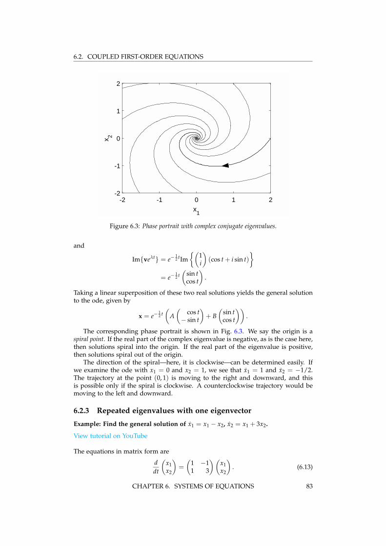
6.2. COUPLED FIRST-ORDER EQUATIONS
The ansatz x = veλt leads to the characteristic equation
0 = det (A − λI)
= λ2 − 4λ + 4
= (λ − 2)2.
Therefore, λ = 2 is a repeated eigenvalue. The associated eigenvector is found from−v1 − v2 = 0, or v2 = −v1; and normalizing with v1 = 1, we have
λ = 2, v =
(1
−1
).
We have thus found a single solution to the ode, given by
x1(t) = c1
(1
−1
)e2t,
and we need to find the missing second solution to be able to satisfy the initialconditions. An ansatz of t times the first solution is tempting, but will fail. Here, wewill cheat and find the missing second solution by solving the equivalent second-order, homogeneous, constant-coefficient differential equation.
We already know that this second-order differential equation for x1(t) has acharacteristic equation with a degenerate eigenvalue given by λ = 2. Therefore, thegeneral solution for x1 is given by
x1(t) = (c1 + tc2)e2t.
Since from the first differential equation, x2 = x1 − x1, we compute
x1 =(2c1 + (1 + 2t)c2
)e2t,
so that
x2 = x1 − x1
= (c1 + tc2)e2t −(2c1 + (1 + 2t)c2
)e2t
= −c1e2t + c2(−1 − t)e2t.
Combining our results for x1 and x2, we have therefore found(x1x2
)= c1
(1
−1
)e2t + c2
[(0
−1
)+
(1
−1
)t]
e2t.
Our missing linearly independent solution is thus determined to be
x(t) = c2
[(0
−1
)+
(1
−1
)t]
e2t. (6.14)
The second term of (6.14) is just t times the first solution; however, this is notsufficient. Indeed, the correct ansatz to find the second solution directly is given by
x = (w + tv) eλt, (6.15)
84 CHAPTER 6. SYSTEMS OF EQUATIONS
6.2. COUPLED FIRST-ORDER EQUATIONS
-2 -1 0 1 2
x1
-2
-1
0
1
2
x 2
Figure 6.4: Phase portrait with only one eigenvector.
where λ and v is the eigenvalue and eigenvector of the first solution, and w is anunknown vector to be determined. To illustrate this direct method, we substitute(6.15) into x = Ax, assuming Av = λv . Canceling the exponential, we obtain
v + λ (w + tv) = Aw + λtv.
Further canceling the common term λtv and rewriting yields
(A − λI)w = v. (6.16)
If A has only a single linearly independent eigenvector v, then (6.16) can be solvedfor w (otherwise, it cannot). Using A, λ and v of our present example, (6.16) is thesystem of equations given by(
−1 −11 1
)(w1w2
)=
(1
−1
).
The first and second equation are the same, so that w2 = −(w1 + 1). Therefore,
w =
(w1
−(w1 + 1)
)= w1
(1
−1
)+
(0
−1
).
Notice that the first term repeats the first found solution, i.e., a constant times theeigenvector, and the second term is new. We therefore take w1 = 0 and obtain
w =
(0
−1
),
as before.The phase portrait for this ode is shown in Fig. 6.4. The dark line is the single
eigenvector v of the matrix A. When there is only a single eigenvector, the origin iscalled an improper node.
CHAPTER 6. SYSTEMS OF EQUATIONS 85

6.3. NORMAL MODES
6.3 Normal modes
View tutorials on YouTube: Part 1 Part 2
We now consider an application of the eigenvector analysis to the coupled mass-spring system shown in Fig. 6.5. The position variables x1 and x2 are measuredfrom the equilibrium positions of the masses. Hooke’s law states that the springforce is linearly proportional to the extension length of the spring, measured fromequilibrium. By considering the extension of the spring and the sign of the force,we write Newton’s law F = ma separately for each mass:
mx1 = −kx1 − K(x1 − x2),mx2 = −kx2 − K(x2 − x1).
Further rewriting by collecting terms proportional to x1 and x2 yields
mx1 = −(k + K)x1 + Kx2,mx2 = Kx1 − (k + K)x2.
The equations for the coupled mass-spring system form a system of two second-order linear homogeneous odes. In matrix form, mx = Ax, or explicitly,
md2
dt2
(x1x2
)=
(−(k + K) K
K −(k + K)
)(x1x2
). (6.17)
In analogy to a system of first-order equations, we try the ansatz x = vert, and uponsubstitution into (6.17) we obtain the eigenvalue problem Av = λv, with λ = mr2.The eigenvalues are determined by solving the characteristic equation
0 = det (A − λI)
=
∣∣∣∣−(k + K)− λ KK −(k + K)− λ
∣∣∣∣= (λ + k + K)2 − K2.
The solution for λ isλ = −k − K ± K,
and the two eigenvalues are
λ1 = −k, λ2 = −(k + 2K).
The corresponding values of r in our ansatz x = vert, with r = ±√
λ/m, are
r1 = i√
k/m, r1, r2 = i√(k + 2K)/m, r2.
Since the values of r are pure imaginary, we know that x1(t) and x2(t) will oscillatewith angular frequencies ω1 = Im{r1} and ω2 = Im{r2}, that is,
ω1 =√
k/m, ω2 =√(k + 2K)/m.
The positions of the oscillating masses in general contain time dependencies of theform sin ω1t, cos ω1t, and sin ω2t, cos ω2t.
86 CHAPTER 6. SYSTEMS OF EQUATIONS

6.3. NORMAL MODES
m m
k kK
x1 x2Figure 6.5: Coupled harmonic oscillators.
It is of further interest to determine the eigenvectors, or so-called normal modesof oscillation, associated with the two distinct angular frequencies. With specificinitial conditions proportional to an eigenvector, the mass will oscillate with a singlefrequency. The eigenvector with eigenvalue λ1 satisfies
−Kv11 + Kv12 = 0,
so that v11 = v12. The normal mode with frequency ω1 =√
k/m thus follows amotion where x1 = x2. Referring to Fig. 6.5, during this motion the center springlength does not change, which is why the frequency of oscillation is independentof K.
Next, we determine the eigenvector with eigenvalue λ2:
Kv21 + Kv22 = 0,
so that v21 = −v22. The normal mode with frequency ω2 =√(k + 2K)/m thus
follows a motion where x1 = −x2. Again referring to Fig. 6.5, during this motionthe two equal masses symmetrically push or pull against each side of the middlespring.
A general solution for x(t) can be constructed from the eigenvalues and eigen-vectors. Our ansatz was x = vert, and for each of two eigenvectors v, we have apair of complex conjugate values for r. Accordingly, we first apply the principle ofsuperposition to obtain four real solutions, and then apply the principle again toobtain the general solution. With ω1 =
√k/m and ω2 =
√(k + 2K)/m, the general
solution is given by(x1x2
)=
(11
)(A cos ω1t + B sin ω1t) +
(1
−1
)(C cos ω2t + D sin ω2t) ,
where the now real constants A, B, C, and D can be determined from the fourindependent initial conditions, x1(0), x2(0), x1(0), and x2(0).
CHAPTER 6. SYSTEMS OF EQUATIONS 87
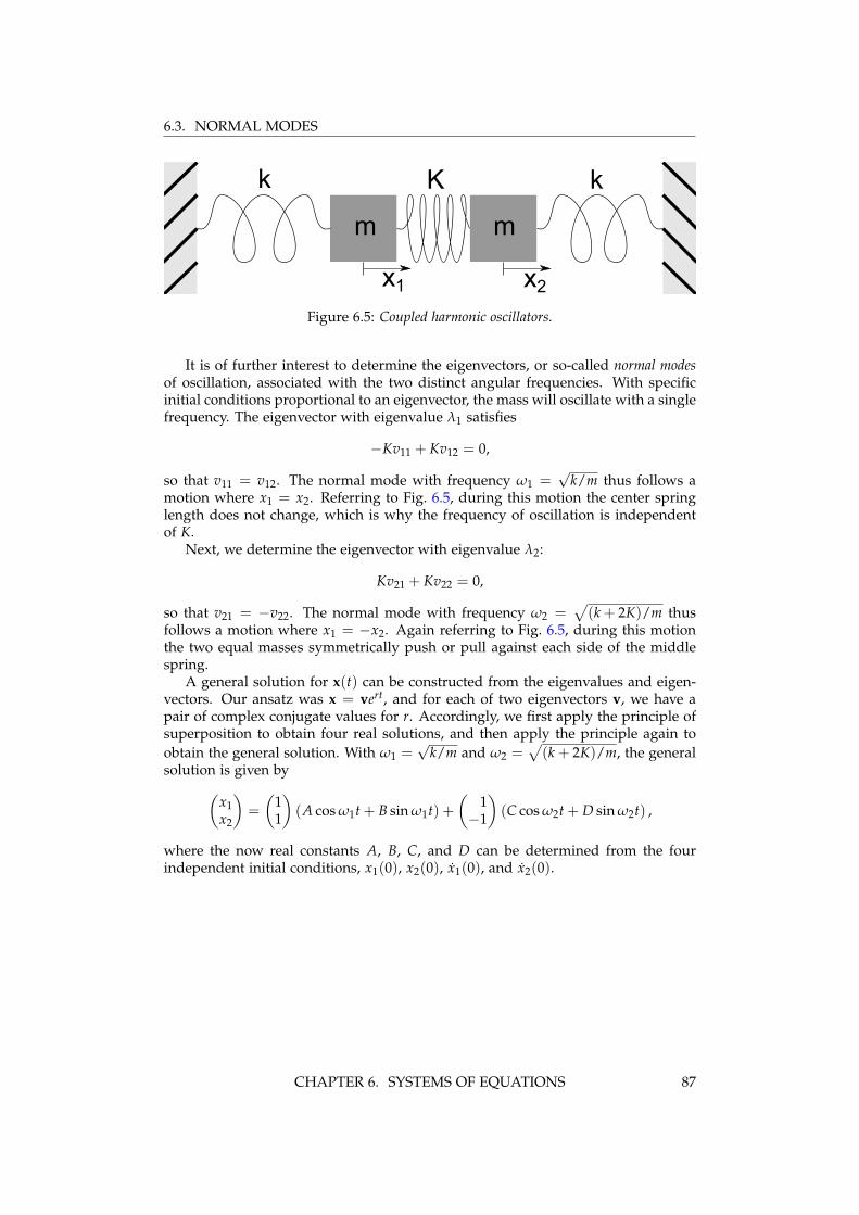
6.3. NORMAL MODES
88 CHAPTER 6. SYSTEMS OF EQUATIONS

Chapter 7
Nonlinear differentialequations and bifurcationtheory
Reference: Strogatz, Sections 2.2, 2.4, 3.1, 3.2, 3.4, 6.3, 6.4, 8.2
We now turn our attention to nonlinear differential equations. In particular, westudy how small changes in the parameters of a system can result in qualitativechanges in the dynamics. These qualitative changes in the dynamics are calledbifurcations. To understand bifurcations, we first need to understand the conceptsof fixed points and stability.
7.1 Fixed points and stability
7.1.1 One dimension
View tutorial on YouTube
Consider the one-dimensional differential equation for x = x(t) given by
x = f (x). (7.1)
We say that x* is a fixed point, or equilibrium point, of (7.1) if f (x*) = 0. At the fixedpoint, x = 0. The terminology fixed point is used since the solution to (7.1) withinitial condition x(0) = x* is x(t) = x* for all time t.
A fixed point, however, can be stable or unstable. A fixed point is said to bestable if a small perturbation of the solution from the fixed point decays in time; it issaid to be unstable if a small perturbation grows in time. We can determine stabilityby a linear analysis. Let x = x* + ε(t), where ε represents a small perturbation ofthe solution from the fixed point x*. Because x* is a constant, x = ε; and becausex* is a fixed point, f (x*) = 0. Taylor series expanding about ε = 0, we have
ε = f (x* + ε)
= f (x*) + ε f ′(x*) + . . .
= ε f ′(x*) + . . . .
The omitted terms in the Taylor series expansion are proportional to ε2, and can bemade negligible over a short time interval with respect to the kept term, propor-tional to ε, by taking ε(0) sufficiently small. Therefore, at least over short times,the differential equation to be considered, ε = f ′(x*)ε, is linear and has by now thefamiliar solution
ε(t) = ε(0)e f ′(x*)t.
89

7.1. FIXED POINTS AND STABILITY
The perturbation of the fixed point solution x(t) = x* thus decays exponentiallyif f ′(x*) < 0, and we say the fixed point is stable. If f ′(x*) > 0, the perturbationgrows exponentially and we say the fixed point is unstable. If f ′(x*) = 0, we saythe fixed point is marginally stable, and the next higher-order term in the Taylorseries expansion must be considered.
Example: Find all the fixed points of the logistic equation x = x(1 − x) anddetermine their stability.
There are two fixed points at which x = 0, given by x* = 0 and x* = 1. Stabilityof these equilibrium points may be determined by considering the derivative off (x) = x(1 − x). We have f ′(x) = 1 − 2x. Therefore, f ′(0) = 1 > 0 so that x* = 0 isan unstable fixed point, and f ′(1) = −1 < 0 so that x* = 1 is a stable fixed point.Indeed, we have previously found that all solutions approach the stable fixed pointasymptotically.
7.1.2 Two dimensionsView tutorial on YouTube
The idea of fixed points and stability can be extended to higher-order systems ofodes. Here, we consider a two-dimensional system and will need to make use ofthe two-dimensional Taylor series expansion of a function F(x, y) about the origin.In general, the Taylor series of F(x, y) is given by
F(x, y) = F + x∂F∂x
+ y∂F∂y
+12
(x2 ∂2F
∂x2 + 2xy∂2F
∂x∂y+ y2 ∂2F
∂y2
)+ . . . ,
where the function F and all of its partial derivatives on the right-hand-side areevaluated at the origin. Note that the Taylor series is constructed so that all partialderivatives of the left-hand-side match those of the right-hand-side at the origin.
We now consider the two-dimensional system given by
x = f (x, y), y = g(x, y). (7.2)
The point (x*, y*) is said to be a fixed point of (7.2) if f (x*, y*) = 0 and g(x*, y*) = 0.Again, the local stability of a fixed point can be determined by a linear analysis.We let x(t) = x* + ε(t) and y(t) = y* + δ(t), where ε and δ are small independentperturbations from the fixed point. Making use of the two dimensional Taylor seriesof f (x, y) and g(x, y) about the fixed point, or equivalently about (ε, δ) = (0, 0), wehave
ε = f (x* + ε, y* + δ)
= f + ε∂ f∂x
+ δ∂ f∂y
+ . . .
= ε∂ f∂x
+ δ∂ f∂y
+ . . . .
δ = g(x* + ε, y* + δ)
= g + ε∂g∂x
+ δ∂g∂y
+ . . .
= ε∂g∂x
+ δ∂g∂y
+ . . . ,
90 CHAPTER 7. NONLINEAR DIFFERENTIAL EQUATIONS

7.1. FIXED POINTS AND STABILITY
0 0.5 1 1.5 2 2.5 3 3.5
x
0
0.5
1
1.5
2
2.5
y
Figure 7.1: Phase portrait for two-dimensional nonlinear system.
where in the Taylor series f , g and all their partial derivatives are evaluated at thefixed point (x*, y*). Neglecting higher-order terms in the Taylor series, we thushave a system of odes for the perturbation, given in matrix form as
ddt
(εδ
)=
( ∂ f∂x
∂ f∂y
∂g∂x
∂g∂y
)(εδ
). (7.3)
The two-by-two matrix in (7.3) is called the Jacobian matrix at the fixed point. Aneigenvalue analysis of the Jacobian matrix will typically yield two eigenvalues λ1and λ2. These eigenvalues may be real and distinct, complex conjugate pairs, orrepeated. The fixed point is stable (all perturbations decay exponentially) if botheigenvalues have negative real parts. The fixed point is unstable (some perturba-tions grow exponentially) if at least one of the eigenvalues has a positive real part.Fixed points can be further classified as stable or unstable nodes, unstable saddlepoints, stable or unstable spiral points, or stable or unstable improper nodes.
Example: Find all the fixed points of the nonlinear system x = x(3 − x − 2y),y = y(2 − x − y), and determine their stability.
View tutorial on YouTube
The fixed points are determined by solving
f (x, y) = x(3 − x − 2y) = 0, g(x, y) = y(2 − x − y) = 0.
Evidently, (x, y) = (0, 0) is a fixed point. On the one hand, if only x = 0, thenthe equation g(x, y) = 0 yields y = 2. On the other hand, if only y = 0, then theequation f (x, y) = 0 yields x = 3. If both x and y are nonzero, then we must solvethe linear system
x + 2y = 3, x + y = 2,
CHAPTER 7. NONLINEAR DIFFERENTIAL EQUATIONS 91
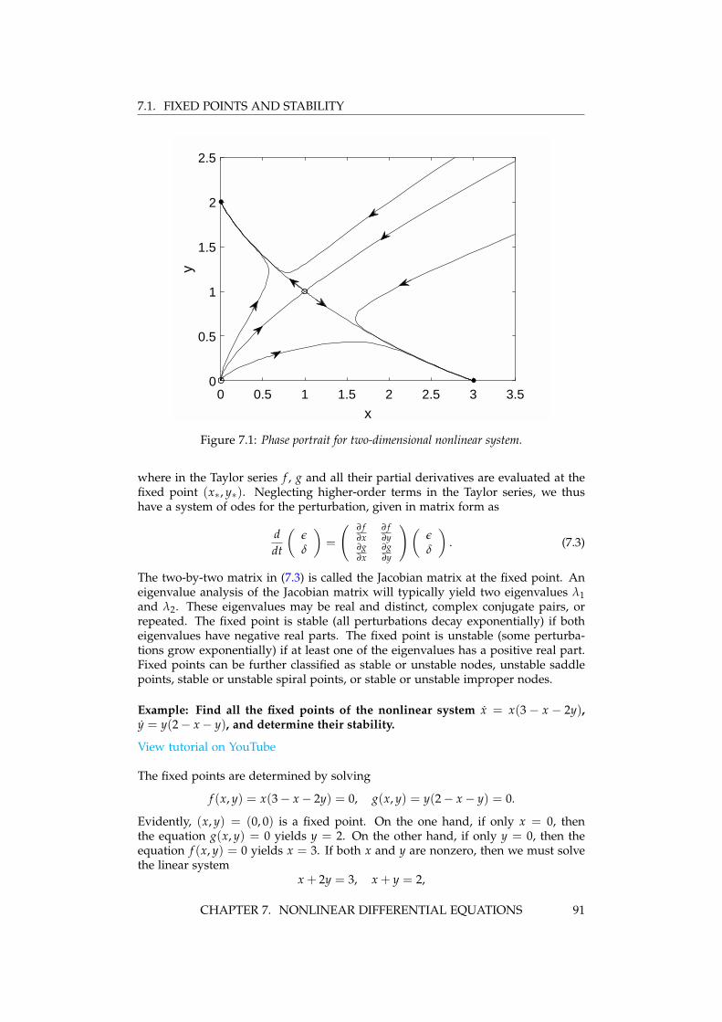
7.1. FIXED POINTS AND STABILITY
and the solution is easily found to be (x, y) = (1, 1). Hence, we have determinedthe four fixed points (x*, y*) = (0, 0), (0, 2), (3, 0), (1, 1). The Jacobian matrix isgiven by ( ∂ f
∂x∂ f∂y
∂g∂x
∂g∂y
)=
(3 − 2x − 2y −2x
−y 2 − x − 2y
).
Stability of the fixed points may be considered in turn. With J* the Jacobian matrixevaluated at the fixed point, we have
(x*, y*) = (0, 0) : J* =(
3 00 2
).
The eigenvalues of J* are λ = 3, 2 so that the fixed point (0, 0) is an unstable node.Next,
(x*, y*) = (0, 2) : J* =(
−1 0−2 −2
).
The eigenvalues of J* are λ = −1,−2 so that the fixed point (0, 2) is a stable node.Next,
(x*, y*) = (3, 0) : J* =(
−3 −60 −1
).
The eigenvalues of J* are λ = −3,−1 so that the fixed point (3, 0) is also a stablenode. Finally,
(x*, y*) = (1, 1) : J* =(
−1 −2−1 −1
).
The characteristic equation of J* is given by (−1−λ)2 − 2 = 0, so that λ = −1±√
2.Since one eigenvalue is negative and the other positive the fixed point (1, 1) is anunstable saddle point. From our analysis of the fixed points, one can expect that allsolutions will asymptote to one of the stable fixed points (0, 2) or (3, 0), dependingon the initial conditions.
It is of interest to sketch the phase portrait for this nonlinear system. The eigen-vectors associated with the unstable saddle point (1, 1) determine the directions ofthe flow into and away from this fixed point. The eigenvector associated with thepositive eigenvalue λ1 = −1 +
√2 can be determined from the first equation of
(J* − λ1I)v1 = 0, or
−√
2v11 − 2v12 = 0,
so that v12 = −(√
2/2)v11. The eigenvector associated with the negative eigenvalueλ1 = −1 −
√2 satisfies v22 = (
√2/2)v21. The eigenvectors give the slope of the
lines with origin at the fixed point for incoming (negative eigenvalue) and outgo-ing (positive eigenvalue) trajectories. The outgoing trajectories have negative slope−√
2/2 and the incoming trajectories have positive slope√
2/2. A rough sketch ofthe phase portrait can be made by hand (as demonstrated in class). Here, a com-puter generated plot obtained from numerical solution of the nonlinear coupledodes is presented in Fig. 7.1. The curve starting from the origin and at infinity,and terminating at the unstable saddle point is called the separatrix. This curveseparates the phase space into two regions: initial conditions for which the solutionasymptotes to the fixed point (0, 2), and initial conditions for which the solutionasymptotes to the fixed point (3, 0).
92 CHAPTER 7. NONLINEAR DIFFERENTIAL EQUATIONS
7.2. ONE-DIMENSIONAL BIFURCATIONS
→ ← →
r<0
→ →
r=0 r>0
dx/dt
x
(a)
(b)x
*
r
Figure 7.2: Saddlenode bifurcation. (a) x versus x; (b) bifurcation diagram.
7.2 One-dimensional bifurcations
A bifurcation occurs in a nonlinear differential equation when a small change ina parameter results in a qualitative change in the long-time solution. Examples ofbifurcations are when fixed points are created or destroyed, or change their stability.
We now consider four classic bifurcations of one-dimensional nonlinear differen-tial equations: saddle-node bifurcation, transcritical bifurcation, supercritical pitch-fork bifurcation, and subcritical pitchfork bifurcation. The corresponding differen-tial equation will be written as
x = fr(x),
where the subscript r represents a parameter that results in a bifurcation whenvaried across zero. The simplest differential equations that exhibit these bifurcationsare called the normal forms, and correspond to a local analysis (i.e., Taylor seriesexpansion) of more general differential equations around the fixed point, togetherwith a possible rescaling of x.
7.2.1 Saddle-node bifurcationView tutorial on YouTube
The saddle-node bifurcation results in fixed points being created or destroyed. Thenormal form for a saddle-node bifurcation is given by
x = r + x2.
The fixed points are x* = ±√−r. Clearly, two real fixed points exist when r < 0
and no real fixed points exist when r > 0. The stability of the fixed points when
CHAPTER 7. NONLINEAR DIFFERENTIAL EQUATIONS 93

7.2. ONE-DIMENSIONAL BIFURCATIONS
← → ←
r<0
dx/dt
x
(a)
← ←
r=0
←← →
r>0
x*
r
(b)
Figure 7.3: Transcritical bifurcation. (a) x versus x; (b) bifurcation diagram.
r < 0 are determined by the derivative of f (x) = r + x2, given by f ′(x) = 2x.Therefore, the negative fixed point is stable and the positive fixed point is unstable.
Graphically, we can illustrate this bifurcation in two ways. First, in Fig. 7.2(a),we plot x versus x for the three parameter values corresponding to r < 0, r = 0 andr > 0. The values at which x = 0 correspond to the fixed points, and arrows aredrawn indicating how the solution x(t) evolves (to the right if x > 0 and to the leftif x < 0). The stable fixed point is indicated by a filled circle and the unstable fixedpoint by an open circle. Note that when r = 0, solutions converge to the origin fromthe left, but diverge from the origin on the right. Second, in Fig. 7.2(b), we plot abifurcation diagram illustrating the fixed point x* versus the bifurcation parameterr. The stable fixed point is denoted by a solid line and the unstable fixed point bya dashed line. Note that the two fixed points collide and annihilate at r = 0, andthere are no fixed points for r > 0.
7.2.2 Transcritical bifurcation
View tutorial on YouTube
A transcritical bifurcation occurs when there is an exchange of stabilities betweentwo fixed points. The normal form for a transcritical bifurcation is given by
x = rx − x2.
The fixed points are x* = 0 and x* = r. The derivative of the right-hand-side isf ′(x) = r − 2x, so that f ′(0) = r and f ′(r) = −r. Therefore, for r < 0, x* = 0is stable and x* = r is unstable, while for r > 0, x* = r is stable and x* = 0 is
94 CHAPTER 7. NONLINEAR DIFFERENTIAL EQUATIONS

7.2. ONE-DIMENSIONAL BIFURCATIONS
→ ←
r<0
dx/dt
x
(a)
→ ←
r=0
←→ ← →
r>0
x*
r
(b)
Figure 7.4: Supercritical pitchfork bifurcation. (a) x versus x; (b) bifurcation diagram.
unstable. The two fixed points thus exchange stability as r passes through zero.The transcritical bifurcation is illustrated in Fig. 7.3.
7.2.3 Supercritical pitchfork bifurcation
View tutorial on YouTube
The pitchfork bifurcations occur in physical models where fixed points appear anddisappear in pairs due to some intrinsic symmetry of the problem. Pitchfork bi-furcations can come in one of two types. In the supercritical bifurcation, a pair ofstable fixed points are created at the bifurcation (or critical) point and exist after(super) the bifurcation. In the subcritical bifurcation, a pair of unstable fixed pointsare created at the bifurcation point and exist before (sub) the bifurcation.
The normal form for the supercritical pitchfork bifurcation is given by
x = rx − x3.
Note that the linear term results in exponential growth when r > 0 and the non-linear term stabilizes this growth. The fixed points are x* = 0 and x* = ±
√r, the
latter fixed points existing only when r > 0. The derivative of f is f ′(x) = r − 3x2
so that f ′(0) = r and f ′(±√
r) = −2r. Therefore, the fixed point x* = 0 is stable forr < 0 and unstable for r > 0 while the fixed points x = ±
√r exist and are stable for
r > 0. Notice that the fixed point x* = 0 becomes unstable as r crosses zero and twonew stable fixed points x* = ±
√r are born. The supercritical pitchfork bifurcation
is illustrated in Fig. 7.4.
CHAPTER 7. NONLINEAR DIFFERENTIAL EQUATIONS 95

7.2. ONE-DIMENSIONAL BIFURCATIONS
x*
r
Figure 7.5: Subcritical pitchfork bifurcation.
7.2.4 Subcritical pitchfork bifurcationView tutorial on YouTube
In the subcritical case, the cubic term is destabilizing. The normal form (to orderx3) is
x = rx + x3.
The fixed points are x* = 0 and x* = ±√−r, the latter fixed points existing only
when r ≤ 0. The derivative of the right-hand-side is f ′(x) = r+ 3x2 so that f ′(0) = rand f ′(±
√−r) = −2r. Therefore, the fixed point x* = 0 is stable for r < 0 and
unstable for r > 0 while the fixed points x = ±√−r exist and are unstable for
r < 0. There are no stable fixed points when r > 0.The absence of stable fixed points for r > 0 indicates that the neglect of terms of
higher-order in x than x3 in the normal form may be unwarranted. Keeping to theintrinsic symmetry of the equations (only odd powers of x) we can add a stabilizingnonlinear term proportional to x5. The extended normal form (to order x5) is
x = rx + x3 − x5,
and is somewhat more difficult to analyze. The fixed points are solutions of
x(r + x2 − x4) = 0.
The fixed point x* = 0 exists for all r, and four additional fixed points can be foundfrom the solutions of the quadratic equation in x2:
x* = ±√
12(1 ±
√1 + 4r).
These fixed points exist only if x* is real. Clearly, for the inner square-root to bereal, r ≥ −1/4. Also observe that 1 −
√1 + 4r becomes negative for r > 0. We thus
have three intervals in r to consider, and these regions and their fixed points are
r < −14
: x* = 0 (one fixed point);
−14
< r < 0 : x* = 0, x* = ±√
12(1 ±
√1 + 4r) (five fixed points);
r > 0 : x* = 0, x* = ±√
12(1 +
√1 + 4r) (three fixed points).
96 CHAPTER 7. NONLINEAR DIFFERENTIAL EQUATIONS

7.2. ONE-DIMENSIONAL BIFURCATIONS
Stability is determined from f ′(x) = r + 3x2 − 5x4. Now, f ′(0) = r so x* = 0 isstable for r < 0 and unstable for r > 0. The calculation for the other four roots canbe simplified by noting that x* satisfies r + x2
* − x4* = 0, or x4
* = r + x2*. Therefore,
f ′(x*) = r + 3x2* − 5x4
*
= r + 3x2* − 5(r + x2
*)
= −4r − 2x2*
= −2(2r + x2*).
With x2* =
12 (1 ±
√1 + 4r), we have
f ′(x*) = −2(
2r +12(1 ±
√1 + 4r)
)= −
((1 + 4r)±
√1 + 4r
)= −
√1 + 4r
(√1 + 4r ± 1
).
Clearly, the plus root is always stable since f ′(x*) < 0. The minus root exists onlyfor − 1
4 < r < 0 and is unstable since f ′(x*) > 0. We summarize the stability of thevarious fixed points:
r < −14
: x* = 0 (stable);
−14
< r < 0 : x* = 0, (stable)
x* = ±√
12(1 +
√1 + 4r) (stable);
x* = ±√
12(1 −
√1 + 4r) (unstable);
r > 0 : x* = 0 (unstable)
x* = ±√
12(1 +
√1 + 4r) (stable).
The bifurcation diagram is shown in Fig. 7.5, and consists of a subcritical pitch-fork bifurcation at r = 0 and two saddle-node bifurcations at r = −1/4. We canimagine what happens to x as r increases from negative values, supposing there issome small noise in the system so that x = x(t) will diverge from unstable fixedpoints. For r < −1/4, the equilibrium value of x is x* = 0. As r increases intothe range −1/4 < r < 0, x will remain at x* = 0. However, a catastrophe occursas soon as r > 0. The x* = 0 fixed point becomes unstable and the solution willjump up (or down) to the only remaining stable fixed point. Such behavior is calleda jump bifurcation. A similar catastrophe can happen as r decreases from positivevalues. In this case, the jump occurs as soon as r < −1/4.
Since the stable equilibrium value of x depends on whether we are increasing ordecreasing r, we say that the system exhibits hysteresis. The existence of a subcriti-cal pitchfork bifurcation can be very dangerous in engineering applications since asmall change in a problem’s parameters can result in a large change in the equilib-rium state. Physically, this can correspond to a collapse of a structure, or the failureof a component.
CHAPTER 7. NONLINEAR DIFFERENTIAL EQUATIONS 97


7.3. TWO-DIMENSIONAL BIFURCATIONS
a Hopf bifurcation. The Hopf bifurcation comes in two types: supercritical Hopfbifurcation and subcritical Hopf bifurcation. For the supercritical Hopf bifurcation,as µ increases slightly above zero, the resulting oscillation around the now unstablefixed point is quickly stabilized at small amplitude. This stable orbit is called a limitcycle. For the subcritical Hopf bifurcation, as µ increases slightly above zero, thelimit cycle immediately jumps to large amplitude.
7.3.1 Supercritical Hopf bifurcation
A simple example of a supercritical Hopf bifurcation can be given in polar coordi-nates:
r = µr − r3,
θ = ω + br2,
where x = r cos θ and y = r sin θ. The parameter µ controls the stability of the fixedpoint at the origin, the parameter ω is the frequency of oscillation near the origin,and the parameter b determines the dependence of the oscillation frequency atlarger amplitude oscillations. Although we include b for generality, our qualitativeanalysis of these equations will be independent of b.
The equation for the radius is of the form of the supercritical pitchfork bifurca-tion. The fixed points are r* = 0 and r* =
õ (note that r > 0), and the former
fixed point is stable for µ < 0 and the latter is stable for µ > 0. The transitionof the eigenvalues of the Jacobian from negative real part to positive real part canbe seen if we transform these equations to cartesian coordinates. We have usingr2 = x2 + y2,
x = r cos θ − θr sin θ
= (µr − r3) cos θ − (ω + br2)r sin θ
= µx − (x2 + y2)x − ωy − b(x2 + y2)y
= µx − ωy − (x2 + y2)(x + by);
y = r sin θ + θr cos θ
= (µr − r3) sin θ + (ω + br2)r cos θ
= µy − (x2 + y2)y + ωx + b(x2 + y2)x
= ωx + µy − (x2 + y2)(y − bx).
The stability of the origin is determined by the Jacobian matrix evaluated at theorigin. The nonlinear terms in the equation vanish and the Jacobian matrix at theorigin is given by
J =(
µ −ωω µ
).
The eigenvalues are the solutions of (µ − λ)2 + ω2 = 0, or λ = µ ± iω. As µ in-creases from negative to positive values, exponentially damped oscillations changeinto exponentially growing oscillations. The nonlinear terms in the equations stabi-lize the growing oscillations into a limit cycle.
100 CHAPTER 7. NONLINEAR DIFFERENTIAL EQUATIONS

7.3. TWO-DIMENSIONAL BIFURCATIONS
7.3.2 Subcritical Hopf bifurcationThe analogous example of a subcritical Hopf bifurcation is given by
r = µr + r3 − r5,
θ = ω + br2.
Here, the equation for the radius is of the form of the subcritical pitchfork bifurca-tion. As µ increases from negative to positive values, the origin becomes unstableand exponentially growing oscillations increase until the radius reaches a stablefixed point far away from the origin. In practice, it may be difficult to tell ana-lytically if a Hopf bifurcation is supercritical or subcritical from the equations ofmotion. Computational solution, however, can quickly distinguish between the twotypes.
CHAPTER 7. NONLINEAR DIFFERENTIAL EQUATIONS 101

7.3. TWO-DIMENSIONAL BIFURCATIONS
102 CHAPTER 7. NONLINEAR DIFFERENTIAL EQUATIONS

Chapter 8
Partial differential equationsReference: Boyce and DiPrima, Chapter 10
Differential equations containing partial derivatives with two or more independentvariables are called partial differential equations (pdes). These equations are offundamental scientific interest but are substantially more difficult to solve, bothanalytically and computationally, than odes.
In this chapter, we begin by deriving two fundamental pdes: the diffusion equa-tion and the wave equation, and show how to solve them with prescribed boundaryconditions using the technique of separation of variables. We then discuss solutionsof the two-dimensional Laplace equation in cartesian and polar coordinates, andfinish with a lengthy discussion of the Schrödinger equation, a partial differentialequation fundamental to both physics and chemistry.
8.1 Derivation of the diffusion equation
To derive the diffusion equation in one spacial dimension, we imagine a still liquidin a long pipe of constant cross sectional area. A small quantity of dye is placed ina cross section of the pipe and allowed to diffuse up and down the pipe. The dyediffuses from regions of higher concentration to regions of lower concentration.
We define u(x, t) to be the concentration of the dye at position x along thepipe, and we wish to find the pde satisfied by u. It is useful to keep track ofthe units of the various quantities involved in the derivation and we introduce thebracket notation [X] to mean the units of X. Relevant dimensional units used in thederivation of the diffusion equation are mass m, length l, and time t. Assuming thatthe dye concentration is uniform in every cross section of the pipe, the dimensionsof concentration used here are [u] = m/l.
The mass of dye in the infinitesimal pipe volume located between position x1and position x2 at time t, with x1 < x < x2, is given to order ∆x = x2 − x1 by
M = u(x, t)∆x.
The mass of dye in this infinitesimal pipe volume changes by diffusion into and outof the cross sectional ends situated at position x1 and x2 (Figure 8.1). We assumethe rate of diffusion is proportional to the concentration gradient, a relationshipknown as Fick’s law of diffusion. Fick’s law of diffusion assumes the mass flux J,with units [J] = m/t across a cross section of the pipe is given by
J = −Dux, (8.1)
where the diffusion constant D > 0 has units [D] = l2/t, and we have used thenotation ux = ∂u/∂x. The mass flux is opposite in sign to the gradient of concen-tration so that the flux is from high concentration to low concentration. The timerate of change in the mass of dye between x1 and x2 is given by the difference be-tween the mass flux into and the mass flux out of the infinitesimal cross sectional
103
8.2. DERIVATION OF THE WAVE EQUATION
J (x2)J (x1)
X1 X2
Figure 8.1: Derivation of the diffusion equation.
volume. A positive mass flux signifies diffusion from left to right. Therefore, thetime rate of change of the dye mass is given by
dMdt
= J(x1, t)− J(x2, t),
or rewriting in terms of u(x, t):
ut(x, t)∆x = D (ux(x2, t)− ux(x1, t)) .
Dividing by ∆x and taking the limit ∆x → 0 results in the diffusion equation:
ut = Duxx.
We note that the diffusion equation is identical to the heat conduction equation,where u is temperature, and the constant D (commonly written as κ) is the thermalconductivity.
8.2 Derivation of the wave equation
To derive the wave equation in one spacial dimension, we imagine an elastic stringthat undergoes small amplitude transverse vibrations. We define u(x, t) to be thevertical displacement of the string from the x-axis at position x and time t, and wewish to find the pde satisfied by u. We define ρ to be the constant mass density ofthe string, T the tension of the string, and θ the angle between the string and thehorizonal line. We consider an infinitesimal string element located between x1 andx2, with ∆x = x2 − x1, as shown in Fig. 8.2. The governing equations are New-ton’s law of motion for the horizontal and vertical acceleration of our infinitesimalstring element, and we assume that the string element only accelerates vertically.Therefore, the horizontal forces must balance and we have
T2 cos θ2 = T1 cos θ1.
The vertical forces result in a vertical acceleration, and with utt the vertical accel-eration of the string element and ρ
√∆x2 + ∆u2 = ρ∆x
√1 + u2
x its mass, where wehave used ux = ∆u/∆x, exact as ∆x → 0, we have
ρ∆x√
1 + u2xutt = T2 sin θ2 − T1 sin θ1.
104 CHAPTER 8. PARTIAL DIFFERENTIAL EQUATIONS

8.3. FOURIER SERIES
Figure 8.2: Derivation of the wave equation.
We now make the assumption of small vibrations, that is ∆u ≪ ∆x, or equivalentlyux ≪ 1. Note that [u] = l so that ux is dimensionless. With this approximation, toleading-order in ux we have
cos θ2 = cos θ1 = 1,
sin θ2 = ux(x2, t), sin θ1 = ux(x1, t),
and √1 + u2
x = 1.
Therefore, to leading order T1 = T2 = T, (i.e., the tension in the string is approxi-mately constant), and
ρ∆xutt = T (ux(x2, t)− ux(x1, t)) .
Dividing by ∆x and taking the limit ∆x → 0 results in the wave equation
utt = c2uxx,
where c2 = T/ρ. Since [T] = ml/t2 and [ρ] = m/l, we have [c2] = l2/t2 so that chas units of velocity.
8.3 Fourier series
View tutorial on YouTube
Our solution of the diffusion and wave equations will require use of a Fourier series.A periodic function f (x) with period 2L, can be represented as a Fourier series inthe form
f (x) =a0
2+
∞
∑n=1
(an cos
nπxL
+ bn sinnπx
L
). (8.2)
CHAPTER 8. PARTIAL DIFFERENTIAL EQUATIONS 105

8.3. FOURIER SERIES
Determination of the coefficients a0, a1, a2, . . . and b1, b2, b3, . . . makes use of or-thogonality relations for sine and cosine. We first define the widely used Kroneckerdelta δnm as
δnm =
{1 if n = m;0 otherwise.
The orthogonality relations for n and m positive integers are then given with com-pact notation as the integration formulas∫ L
−Lcos
(mπxL
)cos
(nπxL
)dx = Lδnm, (8.3)∫ L
−Lsin(mπx
L
)sin(nπx
L
)dx = Lδnm, (8.4)∫ L
−Lcos
(mπxL
)sin(nπx
L
)dx = 0. (8.5)
To illustrate the integration technique used to obtain these results, we derive (8.4)assuming that n and m are positive integers with n = m. Changing variables toξ = πx/L, we obtain∫ L
−Lsin(mπx
L
)sin(nπx
L
)dx
=Lπ
∫ π
−πsin (mξ) sin (nξ)dξ
=L
2π
∫ π
−π
[cos
((m − n)ξ
)− cos
((m + n)ξ
)]dξ
=L
2π
[1
m − nsin((m − n)ξ
)− 1
m + nsin((m + n)ξ
)]π
−π
= 0.
For m = n, however,∫ L
−Lsin2
(nπxL
)dx =
Lπ
∫ π
−πsin2 (nξ)dξ
=L
2π
∫ π
−π
(1 − cos (2nξ)
)dξ
=L
2π
[ξ − 1
2nsin 2nξ
]π
−π
= L.
Integration formulas given by (8.3) and (8.5) can be similarly derived.To determine the coefficient an, we multiply both sides of (8.2) by cos (nπx/L)
with n a nonnegative integer, and change the dummy summation variable from nto m. Integrating over x from −L to L and assuming that the integration can bedone term by term in the infinite sum, we obtain
∫ L
−Lf (x) cos
nπxL
dx =a0
2
∫ L
−Lcos
nπxL
dx
+∞
∑m=1
{am
∫ L
−Lcos
nπxL
cosmπx
Ldx + bm
∫ L
−Lcos
nπxL
sinmπx
Ldx}
.
106 CHAPTER 8. PARTIAL DIFFERENTIAL EQUATIONS
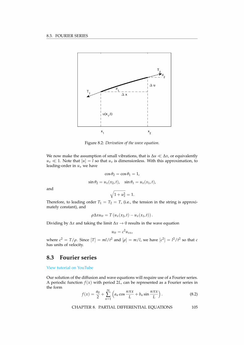
8.4. FOURIER SINE AND COSINE SERIES
If n = 0, then the second and third integrals on the right-hand-side are zero and thefirst integral is 2L so that the right-hand-side becomes La0. If n is a positive integer,then the first and third integrals on the right-hand-side are zero, and the secondintegral is Lδnm. For this case, we have∫ L
−Lf (x) cos
nπxL
dx =∞
∑m=1
Lamδnm
= Lan,
where all the terms in the summation except m = n are zero by virtue of theKronecker delta. We therefore obtain for n = 0, 1, 2, . . .
an =1L
∫ L
−Lf (x) cos
nπxL
dx. (8.6)
To determine the coefficients b1, b2, b3, . . . , we multiply both sides of (8.2) by sin (nπx/L),with n a positive integer, and again change the dummy summation variable from nto m. Integrating, we obtain
∫ L
−Lf (x) sin
nπxL
dx =a0
2
∫ L
−Lsin
nπxL
dx
+∞
∑m=1
{am
∫ L
−Lsin
nπxL
cosmπx
Ldx + bm
∫ L
−Lsin
nπxL
sinmπx
Ldx}
.
Here, the first and second integrals on the right-hand-side are zero, and the thirdintegral is Lδnm so that ∫ L
−Lf (x) sin
nπxL
dx =∞
∑m=1
Lbmδnm
= Lbn.
Hence, for n = 1, 2, 3, . . . ,
bn =1L
∫ L
−Lf (x) sin
nπxL
dx. (8.7)
Our results for the Fourier series of a function f (x) with period 2L are thus givenby (8.2), (8.6) and (8.7).
8.4 Fourier sine and cosine series
View tutorial on YouTube
The Fourier series simplifies if f (x) is an even function such that f (−x) = f (x), oran odd function such that f (−x) = − f (x). Use will be made of the following facts.The function cos (nπx/L) is an even function and sin (nπx/L) is an odd function.The product of two even functions is an even function. The product of two oddfunctions is an even function. The product of an even and an odd function is anodd function. And if g(x) is an even function, then∫ L
−Lg(x)dx = 2
∫ L
0g(x)dx;
CHAPTER 8. PARTIAL DIFFERENTIAL EQUATIONS 107

8.4. FOURIER SINE AND COSINE SERIES
and if g(x) is an odd function, then∫ L
−Lg(x)dx = 0.
We examine in turn the Fourier series for an even or an odd function. First, iff (x) is even, then from (8.6) and (8.7) and our facts about even and odd functions,
an =2L
∫ L
0f (x) cos
nπxL
dx,
bn = 0.(8.8)
The Fourier series for an even function with period 2L is thus given by the Fouriercosine series
f (x) =a0
2+
∞
∑n=1
an cosnπx
L, f (x) even. (8.9)
Second, if f (x) is odd, then
an = 0,
bn =2L
∫ L
0f (x) sin
nπxL
dx;(8.10)
and the Fourier series for an odd function with period 2L is given by the Fouriersine series
f (x) =∞
∑n=1
bn sinnπx
L, f (x) odd. (8.11)
Examples of Fourier series computed numerically can be obtained using theJava applet found at http://www.falstad.com/fourier. Here, we demonstrate ananalytical example.
Example: Determine the Fourier cosine series of the even triangle function rep-resented by Fig. 8.3.
View tutorial on YouTube
The triangle function depicted in Fig. 8.3 is an even function of x with period 2π(i.e., L = π). Its definition on 0 < x < π is given by
f (x) = 1 − 2xπ
.
Because f (x) is even, it can be represented by the Fourier cosine series given by(8.8) and (8.9). The coefficient a0 is
a0 =2π
∫ π
0f (x)dx
=2π
∫ π
0
(1 − 2x
π
)dx
=2π
[x − x2
π
]π
0
= 0.
108 CHAPTER 8. PARTIAL DIFFERENTIAL EQUATIONS

8.4. FOURIER SINE AND COSINE SERIES
0−1
0
1
−2π −π π 2π
Figure 8.3: The even triangle function.
Note that a0/2 is the average value of f (x) over one period, and it is obvious fromFig. 8.3 that this value is zero. The coefficients for n > 0 are
an =2π
∫ π
0f (x) cos (nx)dx
=2π
∫ π
0
(1 − 2x
π
)cos (nx)dx
=2π
∫ π
0cos (nx)dx − 4
π2
∫ π
0x cos (nx)dx
=2
nπsin(nx)
]π
0 − 4π2
{[ xn
sin (nx)]π
0− 1
n
∫ π
0sin (nx)dx
}=
4nπ2
∫ π
0sin (nx)dx
= − 4n2π2 cos (nx)
]π
0
=4
n2π2
(1 − cos (nπ)
).
Since
cos (nπ) =
{−1, if n odd;
1, if n even;
we have
an =
{8/(n2π2), if n odd;0, if n even.
CHAPTER 8. PARTIAL DIFFERENTIAL EQUATIONS 109

8.5. SOLUTION OF THE DIFFUSION EQUATION
The Fourier cosine series for the triangle function is therefore given by
f (x) =8
π2
(cos x +
cos 3x32 +
cos 5x52 + . . .
).
Convergence of this series is rapid. As an interesting aside, evaluation of this seriesat x = 0, using f (0) = 1, yields an infinite series for π2/8:
π2
8= 1 +
132 +
152 + . . . .
With Fourier series now included in our applied mathematics toolbox, we are readyto solve the diffusion and wave equations in bounded domains.
8.5 Solution of the diffusion equation
8.5.1 Homogeneous boundary conditionsWe consider one dimensional diffusion in a pipe of length L, and solve the diffusionequation for the concentration u(x, t),
ut = Duxx, 0 ≤ x ≤ L, t > 0. (8.12)
Both initial and boundary conditions are required for a unique solution. That is, weassume the initial concentration distribution in the pipe is given by
u(x, 0) = f (x), 0 ≤ x ≤ L. (8.13)
Furthermore, we assume that boundary conditions are given at the ends of thepipes. When the concentration value is specified at the boundaries, the boundaryconditions are called Dirichlet boundary conditions. As the simplest example, we as-sume here homogeneous Dirichlet boundary conditions, that is zero concentrationof dye at the ends of the pipe, which could occur if the ends of the pipe open upinto large reservoirs of clear solution,
u(0, t) = 0, u(L, t) = 0, t > 0. (8.14)
We will later also discuss inhomogeneous Dirichlet boundary conditions and homo-geneous Neumann boundary conditions, for which the derivative of the concentrationis specified to be zero at the boundaries. Note that if f (x) is identically zero, thenthe trivial solution u(x, t) = 0 satisfies the differential equation and the initial andboundary conditions and is therefore the unique solution of the problem. In whatfollows, we will assume that f (x) is not identically zero so that we need to find asolution different than the trivial solution.
The solution method we use is called separation of variables. We assume thatu(x, t) can be written as a product of two other functions, one dependent only onposition x and the other dependent only on time t. That is, we make the ansatz
u(x, t) = X(x)T(t). (8.15)
Whether this ansatz will succeed depends on whether the solution indeed has thisform. Substituting (8.15) into (8.12), we obtain
XT′ = DX′′T,
110 CHAPTER 8. PARTIAL DIFFERENTIAL EQUATIONS

8.5. SOLUTION OF THE DIFFUSION EQUATION
which we rewrite by separating the x and t dependence to opposite sides of theequation:
X′′
X=
1D
T′
T.
The left hand side of this equation is independent of t and the right hand side isindependent of x. Both sides of this equation are therefore independent of both xand t and equal to a constant. Introducing −λ as the separation constant, we have
X′′
X=
1D
T′
T= −λ,
and we obtain the two ordinary differential equations
X′′ + λX = 0, T′ + λDT = 0. (8.16)
Because of the boundary conditions, we must first consider the equation for X(x).To solve, we need to determine the boundary conditions at x = 0 and x = L. Now,from (8.14) and (8.15),
u(0, t) = X(0)T(t) = 0, t > 0.
Since T(t) is not identically zero for all t (which would result in the trivial solutionfor u), we must have X(0) = 0. Similarly, the boundary condition at x = L requiresX(L) = 0. We therefore consider the two-point boundary value problem
X′′ + λX = 0, X(0) = X(L) = 0. (8.17)
The equation given by (8.17) is called an ode eigenvalue problem. Clearly, thetrivial solution X(x) = 0 is a solution. Nontrivial solutions exist only for discretevalues of λ. These discrete values of λ and the corresponding functions X(x) arecalled the eigenvalues and eigenfunctions of the differential equation.
Since the form of the general solution of the ode depends on the sign of λ, weconsider in turn the cases λ > 0, λ < 0 and λ = 0. For λ > 0, we write λ = µ2 anddetermine the general solution of
X′′ + µ2X = 0
to beX(x) = A cos µx + B sin µx.
Applying the boundary condition at x = 0, we find A = 0. The boundary conditionat x = L then yields
B sin µL = 0.
The solution B = 0 results in the trivial solution for u and can be ruled out. There-fore, we must have
sin µL = 0,
which is an equation for µ. The solutions are
µ = nπ/L,
where n is an integer. We have thus determined the eigenvalues λ = µ2 > 0 to be
λn = (nπ/L)2 , n = 1, 2, 3, . . . , (8.18)
CHAPTER 8. PARTIAL DIFFERENTIAL EQUATIONS 111

8.5. SOLUTION OF THE DIFFUSION EQUATION
with corresponding eigenfunctions
Xn = sin (nπx/L). (8.19)
For λ < 0, we write λ = −µ2 and determine the general solution of
X′′ − µ2X = 0
to beX(x) = A cosh µx + B sinh µx,
where we have previously introduced the hyperbolic sine and cosine functions in§3.4.1. Applying the boundary condition at x = 0, we find A = 0. The boundarycondition at x = L then yields
B sinh µL = 0,
which for µ = 0 has only the solution B = 0. Therefore, there is no nontrivialsolution for u with λ < 0. Finally, for λ = 0, we have
X′′ = 0,
with general solutionX(x) = A + Bx.
The boundary condition at x = 0 and x = L yields A = B = 0 so again there is nonontrivial solution for u with λ = 0.
We now turn to the equation for T(t). The equation corresponding to the eigen-value λn, using (8.18), is given by
T′ +(
n2π2D/L2)
T = 0,
which has solution proportional to
Tn = e−n2π2Dt/L2. (8.20)
Therefore, multiplying the solutions given by (8.19) and (8.20), we conclude that thefunctions
un(x, t) = sin (nπx/L)e−n2π2Dt/L2(8.21)
satisfy the pde given by (8.12) and the boundary conditions given by (8.14) for everypositive integer n.
The principle of linear superposition for homogeneous linear differential equa-tions then states that the general solution to (8.12) and (8.14) is given by
u(x, t) =∞
∑n=1
bnun(x, t)
=∞
∑n=1
bn sin (nπx/L)e−n2π2Dt/L2.
(8.22)
The final solution step is to satisfy the initial conditions given by (8.13). At t = 0,we have
f (x) =∞
∑n=1
bn sin (nπx/L). (8.23)
112 CHAPTER 8. PARTIAL DIFFERENTIAL EQUATIONS

8.5. SOLUTION OF THE DIFFUSION EQUATION
We immediately recognize (8.23) as a Fourier sine series (8.11) for an odd functionf (x) with period 2L. Equation (8.23) is a periodic extension of our original f (x)defined on 0 ≤ x ≤ L, and is an odd function because of the boundary conditionf (0) = 0. From our solution for the coefficients of a Fourier sine series (8.10), wedetermine
bn =2L
∫ L
0f (x) sin
nπxL
dx. (8.24)
Thus the solution to the diffusion equation with homogeneous Dirichlet boundaryconditions defined by (8.12), (8.13) and (8.14) is given by (8.22) with the bn coeffi-cients computed from (8.24).
Example: Determine the concentration of a dye in a pipe of length L, where thedye has total initial mass M0 and is initially concentrated at the center of thepipe, and the ends of the pipe are held at zero concentration.
The governing equation for concentration is the diffusion equation. We model theinitial concentration of the dye by a delta-function centered at x = L/2, that is,u(x, 0) = f (x) = M0δ(x − L/2). Therefore, from (8.24),
bn =2L
∫ L
0M0δ(x − L
2) sin
nπxL
dx
=2M0
Lsin (nπ/2)
=
2M0/L if n = 1, 5, 9, . . . ;−2M0/L if n = 3, 7, 11, . . . ;0 if n = 2, 4, 6, . . . .
With bn determined, the solution for u(x, t) given by (8.22) can be written as
u(x, t) =2M0
L
∞
∑n=0
(−1)n sin((2n + 1)πx
L
)e−(2n+1)2π2Dt/L2
.
When t ≫ L2/D, the leading-order term in the series is a good approximation andis given by
u(x, t) ≈ 2M0
Lsin (πx/L)e−π2Dt/L2
.
The mass of the dye in the pipe is decreasing in time, diffusing into the reservoirslocated at both ends. The total mass in the pipe at time t can be found from
M(t) =∫ L
0u(x, t)dx,
and since ∫ L
0sin (πx/L)dx =
2Lπ
,
we have for large times
M(t) =4M0
πe−π2Dt/L2
.
CHAPTER 8. PARTIAL DIFFERENTIAL EQUATIONS 113

8.5. SOLUTION OF THE DIFFUSION EQUATION
8.5.2 Inhomogeneous boundary conditionsConsider a diffusion problem where one end of the pipe has dye of concentrationheld constant at C1 and the other held constant at C2, which could occur if the endsof the pipe had large reservoirs of fluid with different concentrations of dye. Withu(x, t) the concentration of dye, the boundary conditions are given by
u(0, t) = C1, u(L, t) = C2, t > 0.
The concentration u(x, t) satisfies the diffusion equation with diffusivity D:
ut = Duxx.
If we try to solve this problem directly using separation of variables, we will runinto trouble. Applying the inhomogeneous boundary condition at x = 0 directly tothe ansatz u(x, t) = X(x)T(t) results in
u(0, t) = X(0)T(t) = C1;
so thatX(0) = C1/T(t).
However, our separation of variables ansatz assumes X(x) to be independent of t!We therefore say that inhomogeneous boundary conditions are not separable.
The proper way to solve a problem with inhomogeneous boundary conditionsis to transform it into another problem with homogeneous boundary conditions.As t → ∞, we assume that a stationary concentration distribution v(x) will attain,independent of t. Since v(x) must satisfy the diffusion equation, we have
v′′(x) = 0, 0 ≤ x ≤ L,
with general solutionv(x) = A + Bx.
Since v(x) must satisfy the same boundary conditions of u(x, t), we have v(0) = C1and v(L) = C2, and we determine A = C1 and B = (C2 − C1)/L.
We now express u(x, t) as the sum of the known asymptotic stationary con-centration distribution v(x) and an unknown transient concentration distributionw(x, t):
u(x, t) = v(x) + w(x, t).Substituting into the diffusion equation, we obtain
∂
∂t(v(x) + w(x, t)) = D
∂2
∂x2 (v(x) + w(x, t))
orwt = Dwxx,
since vt = 0 and vxx = 0. The boundary conditions satisfied by w are
w(0, t) = u(0, t)− v(0) = 0,w(L, t) = u(L, t)− v(L) = 0,
so that w is observed to satisfy homogeneous boundary conditions. If the initialconditions are given by u(x, 0) = f (x), then the initial conditions for w are
w(x, 0) = u(x, 0)− v(x)= f (x)− v(x).
The resulting equations may then be solved for w(x, t) using the technique for ho-mogeneous boundary conditions, and u(x, t) subsequently determined.
114 CHAPTER 8. PARTIAL DIFFERENTIAL EQUATIONS

8.5. SOLUTION OF THE DIFFUSION EQUATION
8.5.3 Pipe with closed endsThere is no diffusion of dye through the ends of a sealed pipe. Accordingly, themass flux of dye through the pipe ends, given by (8.1), is zero so that the boundaryconditions on the dye concentration u(x, t) becomes
ux(0, t) = 0, ux(L, t) = 0, t > 0, (8.25)
which are known as homogeneous Neumann boundary conditions. Again, we ap-ply the method of separation of variables and as before, we obtain the two ordinarydifferential equations given by (8.16). Considering first the equation for X(x), theappropriate boundary conditions are now on the first derivative of X(x), and wemust solve
X′′ + λX = 0, X′(0) = X′(L) = 0. (8.26)
Again, we consider in turn the cases λ > 0, λ < 0 and λ = 0. For λ > 0, we writeλ = µ2 and determine the general solution of (8.26) to be
X(x) = A cos µx + B sin µx,
so that taking the derivative
X′(x) = −µA sin µx + µB cos µx.
Applying the boundary condition X′(0) = 0, we find B = 0. The boundary condi-tion at x = L then yields
−µA sin µL = 0.
The solution A = 0 results in the trivial solution for u and can be ruled out. There-fore, we must have
sin µL = 0,
with solutionsµ = nπ/L,
where n is an integer. We have thus determined the eigenvalues λ = µ2 > 0 to be
λn = (nπ/L)2 , n = 1, 2, 3, . . . , (8.27)
with corresponding eigenfunctions
Xn = cos (nπx/L). (8.28)
For λ < 0, we write λ = −µ2 and determine the general solution of (8.26) to be
X(x) = A cosh µx + B sinh µx,
so that taking the derivative
X′(x) = µA sinh µx + µB cosh µx.
Applying the boundary condition X′(0) = 0 yields B = 0. The boundary conditionX′(L) = 0 then yields
µA sinh µL = 0,
which for µ = 0 has only the solution A = 0. Therefore, there is no nontrivialsolution for u with λ < 0. Finally, for λ = 0, the general solution of (8.26) is
X(x) = A + Bx,
CHAPTER 8. PARTIAL DIFFERENTIAL EQUATIONS 115

8.5. SOLUTION OF THE DIFFUSION EQUATION
so that taking the derivativeX′(x) = B.
The boundary condition X′(0) = 0 yields B = 0; X′(L) = 0 is then trivially satisfied.Therefore, we have an additional eigenvalue and eigenfunction given by
λ0 = 0, X0(x) = 1,
which can be seen as extending the formula obtained for eigenvalues and eigenvec-tors for positive λ given by (8.27) and (8.28) to n = 0.
We now turn to the equation for T(t). The equation corresponding to eigenvalueλn, using (8.27), is given by
T′ +(
n2π2D/L2)
T = 0,
which has solution proportional to
Tn = e−n2π2Dt/L2, (8.29)
valid for n = 0, 1, 2, . . . . Therefore, multiplying the solutions given by (8.28) and(8.29), we conclude that the functions
un(x, t) = cos (nπx/L)e−n2π2Dt/L2(8.30)
satisfy the pde given by (8.12) and the boundary conditions given by (8.25) for everynonnegative integer n.
The principle of linear superposition then yields the general solution as
u(x, t) =∞
∑n=0
cnun(x, t)
=a0
2+
∞
∑n=1
an cos (nπx/L)e−n2π2Dt/L2,
(8.31)
where we have redefined the constants so that c0 = a0/2 and cn = an, n = 1, 2, 3, . . . .The final solution step is to satisfy the initial conditions given by (8.13). At t = 0,we have
f (x) =a0
2+
∞
∑n=1
an cos (nπx/L), (8.32)
which we recognize as a Fourier cosine series (8.9) for an even function f (x) withperiod 2L. We have obtained a cosine series for the periodic extension of f (x)because of the boundary condition f ′(0) = 0, which is satisfied by an even functionwith continuous first derivative. From our solution (8.8) for the coefficients of aFourier cosine series, we determine
an =2L
∫ L
0f (x) cos
nπxL
dx. (8.33)
Thus the solution to the diffusion equation with homogenous Neumann boundaryconditions defined by (8.12), (8.13) and (8.25) is given by (8.31) with the coefficientscomputed from (8.33).
116 CHAPTER 8. PARTIAL DIFFERENTIAL EQUATIONS

8.6. SOLUTION OF THE WAVE EQUATION
Example: Determine the concentration of a dye in a pipe of length L, where thedye has total initial mass M0 and is initially concentrated at the center of thepipe, and the ends of the pipe are sealed
Again we model the initial concentration of the dye by a delta-function centered atx = L/2. From (8.33),
an =2L
∫ L
0M0δ(x − L
2) cos
nπxL
dx
=2M0
Lcos (nπ/2)
=
2M0/L if n = 0, 4, 8, . . . ;−2M0/L if n = 2, 6, 10, . . . ;0 if n = 1, 3, 5, . . . .
The first two terms in the series for u(x, t) are given by
u(x, t) =M0
L
[1 − 2 cos (2πx/L)e−4π2Dt/L2
+ . . .]
.
Notice that as t → ∞, u(x, t) → M0/L: the dye mass is conserved in the pipe (sincethe pipe ends are sealed) and eventually diffused uniformly throughout the pipe oflength L.
8.6 Solution of the wave equation
8.6.1 Plucked stringWe assume an elastic string with fixed ends is plucked like a guitar string. The gov-erning equation for u(x, t), the position of the string from its equilibrium position,is the wave equation
utt = c2uxx, (8.34)
with c2 = T/ρ and with boundary conditions at the string ends located at x = 0and L given by
u(0, t) = 0, u(L, t) = 0. (8.35)
Since the wave equation is second-order in time, initial conditions are required forboth the displacement of the string due to the plucking and the initial velocity ofthe displacement. We assume
u(x, 0) = f (x), ut(x, 0) = 0, 0 ≤ x ≤ L. (8.36)
Again we use the method of separation of variables and try the ansatz
u(x, t) = X(x)T(t). (8.37)
Substitution of our ansatz (8.37) into the wave equation (8.34) and separating vari-ables results in
X′′
X=
1c2
T′′
T= −λ,
yielding the two ordinary differential equations
X′′ + λX = 0, T′′ + λc2T = 0. (8.38)
CHAPTER 8. PARTIAL DIFFERENTIAL EQUATIONS 117

8.6. SOLUTION OF THE WAVE EQUATION
We solve first the equation for X(x). The appropriate boundary conditions for Xare given by
X(0) = 0, X(L) = 0, (8.39)
and we have solved this equation for X(x) previously in §8.5.1 (see (8.17)). A non-trivial solution exists only when λ > 0, and our previously determined solutionwas
λn = (nπ/L)2 , n = 1, 2, 3, . . . , (8.40)
with corresponding eigenfunctions
Xn = sin (nπx/L). (8.41)
With λn specified, the T equation then becomes
T′′n +
n2π2c2
L2 Tn = 0,
with general solution given by
Tn(t) = A cosnπct
L+ B sin
nπctL
. (8.42)
The second of the initial conditions given by (8.36) implies
ut(x, 0) = X(x)T′(0) = 0,
which can be satisfied only if T′(0) = 0. Applying this boundary condition to(8.42), we find B = 0. Combining our solution for Xn(x), (8.41), and Tn(t), we havedetermined that
un(x, t) = sinnπx
Lcos
nπctL
, n = 1, 2, 3, . . .
satisfies the wave equation, the boundary conditions at the string ends, and theassumption of zero initial string velocity. Linear superposition of these solutionsresults in the general solution for u(x, t) of the form
u(x, t) =∞
∑n=1
bn sinnπx
Lcos
nπctL
. (8.43)
The remaining condition to satisfy is the initial displacement of the string, the firstequation of (8.36). We have
f (x) =∞
∑n=1
bn sin (nπx/L),
which is observed to be a Fourier sine series (8.11) for an odd function with period2L. Therefore, the coefficients bn are given by (8.10),
bn =2L
∫ L
0f (x) sin
nπxL
dx, n = 1, 2, 3, . . . . (8.44)
Our solution to the wave equation with plucked string is thus given by (8.43) and(8.44). Notice that the solution is time periodic with period 2L/c. The correspond-ing fundamental frequency is the reciprocal of the period and is given by f = c/2L.From our derivation of the wave equation in §8.2, the velocity c is related to the
118 CHAPTER 8. PARTIAL DIFFERENTIAL EQUATIONS

8.6. SOLUTION OF THE WAVE EQUATION
density of the string ρ and tension of the string T by c2 = T/ρ. Therefore, thefundamental frequency (pitch) of our “guitar string” increases (is raised) with in-creasing tension, decreasing string density, and decreasing string length. Indeed,these are exactly the parameters used to construct, tune and play a guitar.
The wave nature of our solution and the physical significance of the velocity ccan be made more transparent if we make use of the trigonometric identity
sin x cos y =12(sin (x + y) + sin (x − y)
).
With this identity, our solution (8.43) can be rewritten as
u(x, t) =12
∞
∑n=1
bn
(sin
nπ(x + ct)L
+ sinnπ(x − ct)
L
). (8.45)
The first and second sine functions can be interpreted as a traveling wave movingto the left or the right with velocity c. This can be seen by incrementing time,t → t + δ, and observing that the value of the first sine function is unchangedprovided the position is shifted by x → x − cδ, and the second sine function isunchanged provided x → x + cδ. Two waves travelling in opposite directions withequal amplitude results in a standing wave.
8.6.2 Hammered string
In contrast to a guitar string that is plucked, a piano string is hammered. Theappropriate initial conditions for a piano string would be
u(x, 0) = 0, ut(x, 0) = g(x), 0 ≤ x ≤ L. (8.46)
Our solution proceeds as previously, except that now the homogeneous initial con-dition on T(t) is T(0) = 0, so that A = 0 in (8.42). The wave equation solution istherefore
u(x, t) =∞
∑n=1
bn sinnπx
Lsin
nπctL
. (8.47)
Imposition of initial conditions then yields
g(x) =πcL
∞
∑n=1
nbn sinnπx
L.
The coefficient of the Fourier sine series for g(x) is seen to be nπcbn/L, and we have
nπcbn
L=
2L
∫ L
0g(x) sin
nπxL
dx,
or
bn =2
nπc
∫ L
0g(x) sin
nπxL
dx.
8.6.3 General initial conditions
If the initial conditions on u(x, t) are generalized to
u(x, 0) = f (x), ut(x, 0) = g(x), 0 ≤ x ≤ L, (8.48)
CHAPTER 8. PARTIAL DIFFERENTIAL EQUATIONS 119

8.7. THE LAPLACE EQUATION
0 a0
b
x
yu = 0
u = 0
u = 0 u = f(y)
Figure 8.4: Dirichlet problem for the Laplace equation in a rectangle.
then the solution to the wave equation can be determined using the principle oflinear superposition. Suppose v(x, t) is the solution to the wave equation withinitial condition (8.36) and w(x, t) is the solution to the wave equation with initialconditions (8.46). Then we have
u(x, t) = v(x, t) + w(x, t),
since u(x, t) satisfies the wave equation, the boundary conditions, and the initialconditions given by (8.48).
8.7 The Laplace equation
The diffusion equation in two spatial dimensions is
ut = D(uxx + uyy).
The steady-state solution, approached asymptotically in time, has ut = 0 so that thesteady-state solution u = u(x, y) satisfies the two-dimensional Laplace equation
uxx + uyy = 0. (8.49)
We will consider the mathematical problem of solving the two dimensional Laplaceequation inside a rectangular or a circular boundary. The value of u(x, y) will bespecified on the boundaries, defining this problem to be of Dirichlet type.
8.7.1 Dirichlet problem for a rectangleWe consider the Laplace equation (8.49) for the interior of a rectangle 0 < x < a,0 < y < b, (see Fig. 8.4), with boundary conditions
u(x, 0) = 0, u(x, b) = 0, 0 < x < a;u(0, y) = 0, u(a, y) = f (y), 0 ≤ y ≤ b.
120 CHAPTER 8. PARTIAL DIFFERENTIAL EQUATIONS

8.7. THE LAPLACE EQUATION
More general boundary conditions can be solved by linear superposition of solu-tions.
We take our usual ansatz
u(x, y) = X(x)Y(y),
and find after substitution into (8.49),
X′′
X= −Y′′
Y= λ,
with λ the separation constant. We thus obtain the two ordinary differential equa-tions
X′′ − λX = 0, Y′′ + λY = 0.
The homogeneous boundary conditions are X(0) = 0, Y(0) = 0 and Y(b) = 0.We have already solved the equation for Y(y) in §8.5.1, and the solution yields theeigenvalues
λn =(nπ
b
)2, n = 1, 2, 3, . . . ,
with corresponding eigenfunctions
Yn(y) = sinnπy
b.
The remaining X equation and homogeneous boundary condition is therefore
X′′ − n2π2
b2 X = 0, X(0) = 0,
and the solution is the hyperbolic sine function
Xn(x) = sinhnπx
b,
times a constant. Writing un = XnYn, multiplying by a constant and summing overn, yields the general solution
u(x, y) =∞
∑n=0
cn sinhnπx
bsin
nπyb
.
The remaining inhomogeneous boundary condition u(a, y) = f (y) results in
f (y) =∞
∑n=0
cn sinhnπa
bsin
nπyb
,
which we recognize as a Fourier sine series for an odd function with period 2b, andcoefficient cn sinh (nπa/b). The solution for the coefficient is given by
cn =2
b sinh nπab
∫ b
0f (y) sin
nπyb
dy.
CHAPTER 8. PARTIAL DIFFERENTIAL EQUATIONS 121

8.7. THE LAPLACE EQUATION
8.7.2 Dirichlet problem for a circleThe Laplace equation is commonly written symbolically as
∇2u = 0, (8.50)
where ∇2 is called the Laplacian, sometimes denoted as ∆. The Laplacian can bewritten in various coordinate systems, and the choice of coordinate systems usuallydepends on the geometry of the boundaries. Indeed, the Laplace equation is knownto be separable in 13 different coordinate systems! We have solved the Laplaceequation in two dimensions, with boundary conditions specified on a rectangle,using
∇2 =∂2
∂x2 +∂2
∂y2 .
Here we consider boundary conditions specified on a circle, and write the Lapla-cian in polar coordinates by changing variables from cartesian coordinates. Polarcoordinates is defined by the transformation (r, θ) → (x, y):
x = r cos θ, y = r sin θ; (8.51)
and the chain rule gives for the partial derivatives
∂u∂r
=∂u∂x
∂x∂r
+∂u∂y
∂y∂r
,∂u∂θ
=∂u∂x
∂x∂θ
+∂u∂y
∂y∂θ
. (8.52)
After taking the partial derivatives of x and y using (8.51), we can write the trans-formation (8.52) in matrix form as(
∂u/∂r∂u/∂θ
)=
(cos θ sin θ
−r sin θ r cos θ
)(∂u/∂x∂u/∂y
). (8.53)
Inversion of (8.53) can be determined from the following result, commonly provedin a linear algebra class. If
A =
(a bc d
), det A = 0,
then
A−1 =1
det A
(d −b
−c a
).
Therefore, since the determinant of the 2 × 2 matrix in (8.53) is r, we have(∂u/∂x∂u/∂y
)=
(cos θ − sin θ/rsin θ cos θ/r
)(∂u/∂r∂u/∂θ
). (8.54)
Rewriting (8.54) in operator form, we have
∂
∂x= cos θ
∂
∂r− sin θ
r∂
∂θ,
∂
∂y= sin θ
∂
∂r+
cos θ
r∂
∂θ. (8.55)
To find the Laplacian in polar coordinates with minimum algebra, we combine(8.55) using complex variables as
∂
∂x+ i
∂
∂y= eiθ
(∂
∂r+
ir
∂
∂θ
), (8.56)
122 CHAPTER 8. PARTIAL DIFFERENTIAL EQUATIONS

8.7. THE LAPLACE EQUATION
so that the Laplacian may be found by multiplying both sides of (8.56) by its com-plex conjugate, taking care with the computation of the derivatives on the right-hand-side:
∂2
∂x2 +∂2
∂y2 = eiθ(
∂
∂r+
ir
∂
∂θ
)e−iθ
(∂
∂r− i
r∂
∂θ
)=
∂2
∂r2 +1r
∂
∂r+
1r2
∂2
∂θ2 .
We have therefore determined that the Laplacian in polar coordinates is given by
∇2 =∂2
∂r2 +1r
∂
∂r+
1r2
∂2
∂θ2 , (8.57)
which is sometimes written as
∇2 =1r
∂
∂r
(r
∂
∂r
)+
1r2
∂2
∂θ2 .
We now consider the solution of the Laplace equation in a circle with radiusr < a subject to the boundary condition
u(a, θ) = f (θ), 0 ≤ θ ≤ 2π. (8.58)
An additional boundary condition due to the use of polar coordinates is that u(r, θ)is periodic in θ with period 2π. Furthermore, we will also assume that u(r, θ) isfinite within the circle.
The method of separation of variables takes as our ansatz
u(r, θ) = R(r)Θ(θ),
and substitution into the Laplace equation (8.50) using (8.57) yields
R′′Θ +1r
R′Θ +1r2 RΘ′′ = 0,
or
r2 R′′
R+ r
R′
R= −Θ′′
Θ= λ,
where λ is the separation constant. We thus obtain the two ordinary differentialequations
r2R′′ + rR′ − λR = 0, Θ′′ + λΘ = 0.
The Θ equation is solved assuming periodic boundary conditions with period 2π.If λ < 0, then no periodic solution exists. If λ = 0, then Θ can be constant. Ifλ = µ2 > 0, then
Θ(θ) = A cos µθ + B sin µθ,
and the requirement that Θ is periodic with period 2π forces µ to be an integer.Therefore,
λn = n2, n = 0, 1, 2, . . . ,
with corresponding eigenfunctions
Θn(θ) = An cos nθ + Bn sin nθ.
CHAPTER 8. PARTIAL DIFFERENTIAL EQUATIONS 123
8.7. THE LAPLACE EQUATION
The R equation for each eigenvalue λn then becomes
r2R′′ + rR′ − n2R = 0, (8.59)
which is an Euler equation. With the ansatz R = rs, (8.59) reduces to the algebraicequation s(s − 1) + s − n2 = 0, or s2 = n2. Therefore, s = ±n, and there are tworeal solutions when n > 0 and degenerate solutions when n = 0. When n > 0, thesolution for R(r) is
Rn(r) = Arn + Br−n.
The requirement that u(r, θ) is finite in the circle forces B = 0 since r−n becomesunbounded as r → 0. When n = 0, the solution for R(r) is
Rn(r) = A + B ln r,
and again finite u in the circle forces B = 0. Therefore, the solution for n = 0, 1, 2, . . .is Rn = rn. Thus the general solution for u(r, θ) may be written as
u(r, θ) =A0
2+
∞
∑n=1
rn(An cos nθ + Bn sin nθ), (8.60)
where we have separated out the n = 0 solution to write our solution in a formsimilar to the standard Fourier series given by (8.2). The remaining boundary con-dition (8.58) specifies the values of u on the circle of radius a, and imposition of thisboundary condition results in
f (θ) =A0
2+
∞
∑n=1
an(An cos nθ + Bn sin nθ). (8.61)
Equation (8.61) is a Fourier series for the periodic function f (θ) with period 2π, i.e.,L = π in (8.2). The Fourier coefficients an An and anBn are therefore given by (8.6)and (8.7) to be
an An =1π
∫ 2π
0f (φ) cos nφdφ, n = 0, 1, 2, . . . ;
anBn =1π
∫ 2π
0f (φ) sin nφdφ, n = 1, 2, 3, . . . , (8.62)
where we have used φ for the dummy variable of integration.A remarkable fact is that the infinite series solution for u(r, θ) can be summed
explicitly. Substituting (8.62) into (8.60), we obtain
u(r, θ) =1
2π
∫ 2π
0dφ f (φ)
[1 + 2
∞
∑n=1
( ra
)n(cos nθ cos nφ + sin nθ sin nφ)
]
=1
2π
∫ 2π
0dφ f (φ)
[1 + 2
∞
∑n=1
( ra
)ncos n(θ − φ)
].
We can sum the infinite series by writing 2 cos n(θ − φ) = ein(θ−φ) + e−in(θ−φ), and
124 CHAPTER 8. PARTIAL DIFFERENTIAL EQUATIONS

8.8. THE SCHRÖDINGER EQUATION
using the sum of the geometric series ∑∞n=1 zn = z/(1 − z) to obtain
1 + 2∞
∑n=1
( ra
)ncos n(θ − φ) = 1 +
∞
∑n=1
(rei(θ−φ)
a
)n
+∞
∑n=1
(re−i(θ−φ)
a
)n
= 1 +
(rei(θ−φ)
a − rei(θ−φ)+ c.c.
)
=a2 − r2
a2 − 2ar cos (θ − φ) + r2 .
Therefore,
u(r, θ) =a2 − r2
2π
∫ 2π
0
f (φ)a2 − 2ar cos (θ − φ) + r2 dφ,
an integral result for u(r, θ) known as Poisson’s formula. As a trivial example,consider the solution for u(r, θ) if f (θ) = F, a constant. Clearly, u(r, θ) = F satisfiesboth the Laplace equation and the boundary conditions so must be the solution.You can verify that u(r, θ) = F is indeed the solution by showing that
∫ 2π
0
dφ
a2 − 2ar cos (θ − φ) + r2 =2π
a2 − r2 .
8.8 The Schrödinger equation
The Schrödinger equation is the equation of motion for nonrelativistic quantummechanics. This equation is a linear partial differential equation and in simplesituations can be solved using the technique of separation of variables. Luckily, oneof the cases that can be solved analytically is the hydrogen atom. It can be arguedthat the greatest success of classical mechanics was the solution of the Earth-Sunsystem. Similarly, it can be argued that the greatest success of quantum mechanicswas the solution of the electron-proton system. The mathematical solutions of theseclassical and quantum two-body problems rank among the highest achievements ofmankind.
8.8.1 Heuristic derivation of the Schrödinger equation
Nature consists of waves and particles. Early in the twentieth century, light wasdiscovered to act as both a wave and a particle, and quantum mechanics assumesthat matter can also act in both ways.
In general, waves are described by their wavelength λ and frequency ν, or equiv-alently their wavenumber k = 2π/λ and their angular frequency ω = 2πν. ThePlanck-Einstein relations for light postulated that the energy E and momentum pof a light particle, called a photon, is proportional to the angular frequency ω andwavenumber k of the light wave. The proportionality constant is called “h bar”,denoted as h, and is related to the original Planck’s constant h by h = h/2π. ThePlanck-Einstein relations are given by
E = hω, p = hk.
De Broglie in 1924 postulated that matter also follows these relations.
CHAPTER 8. PARTIAL DIFFERENTIAL EQUATIONS 125

8.8. THE SCHRÖDINGER EQUATION
A heuristic derivation of the Schrödinger equation for a particle of mass m andmomentum p constrained to move in one dimension begins with the classical equa-tion
p2
2m+ V(x, t) = E, (8.63)
where p2/2m is the kinetic energy of the mass, V(x, t) is the potential energy, andE is the total energy.
In search of a wave equation, we consider how to write a free wave in onedimension. Using a real function, we could write
Ψ = A cos (kx − ωt + φ), (8.64)
where A is the amplitude and φ is the phase. Or using a complex function, wecould write
Ψ = Cei(kx−ωt), (8.65)
where C is a complex number containing both amplitude and phase.We now rewrite the classical energy equation (8.63) using the Planck-Einstein
relations. After multiplying by a wavefunction, we have
h2
2mk2Ψ(x, t) + V(x, t)Ψ(x, t) = hωΨ(x, t).
We would like to replace k and ω, which refer to the wave characteristics of theparticle, by differential operators acting on the wavefunction Ψ(x, t). If we considerV(x, t) = 0 and the free particle wavefunctions given by (8.64) and (8.65), it is easyto see that to replace both k2 and ω by derivatives we need to use the complex formof the wavefunction and explicitly introduce the imaginary unit i, that is
k2 → − ∂2
∂x2 , ω → i∂
∂t.
Doing this, we obtain the intrinsically complex equation
− h2
2m∂2Ψ∂x2 + V(x, t)Ψ = ih
∂Ψ∂t
,
which is the one-dimensional Schrödinger equation for a particle of mass m in apotential V = V(x, t). This equation is easily generalized to three dimensions andtakes the form
− h2
2m∇2Ψ(x, t) + V(x, t)Ψ(x, t) = ih
∂Ψ(x, t)∂t
, (8.66)
where in Cartesian coordinates the Laplacian ∇2 is written as
∇2 =∂2
∂x2 +∂2
∂y2 +∂2
∂z2 .
The Born interpretation of the wavefunction states that |Ψ(x, t)|2 is the probabil-ity density function of the particle’s location. That is, the spatial integral of |Ψ(x, t)|2over a volume V gives the probability of finding the particle in V at time t. Sincethe particle must be somewhere, the wavefunction for a bound particle is usuallynormalized so that ∫ ∞
−∞
∫ ∞
−∞
∫ ∞
−∞|Ψ(x, y, z; t)|2dx dy dz = 1.
126 CHAPTER 8. PARTIAL DIFFERENTIAL EQUATIONS

8.8. THE SCHRÖDINGER EQUATION
The simple requirements that the wavefunction be normalizable as well as singlevalued admits an analytical solution of the Schrödinger equation for the hydrogenatom.
8.8.2 The time-independent Schrödinger equation
The space and time variables of the time-dependent Schrödinger equation (8.66)can be separated provided the potential function V(x, t) = V(x) is independent oftime. We try Ψ(x, t) = ψ(x) f (t) and obtain
− h2
2mf∇2ψ + V(x)ψ f = ihψ f ′.
Dividing by ψ f , the equation separates as
− h2
2m∇2ψ
ψ+ V(x) = ih
f ′
f.
The left-hand side is independent of t, the right-hand side is independent of x, soboth the left- and right-hand sides must be independent of x and t and equal to aconstant. We call this separation constant E, thereby reintroducing the total energyinto the equation. We now have the two differential equations
f ′ = − iEh
f , − h2
2m∇2ψ + V(x)ψ = Eψ.
The second equation is called the time-independent Schrödinger equation. The firstequation can be easily integrated to obtain
f (t) = e−iEt/h,
which can be multiplied by a arbitrary constant.
8.8.3 Particle in a one-dimensional box
We assume that a particle of mass m is able to move freely in only one dimensionand is confined to the region defined by 0 < x < L. This is perhaps the sim-plest quantum mechanical problem with quantized energy levels. We take as thepotential energy function
V(x) =
{0, 0 < x < L,∞, otherwise,
where we may assume that the particle is forbidden from the region with infinitepotential energy. We will simply take as the boundary conditions on the wavefunc-tion
ψ(0) = ψ(L) = 0. (8.67)
For this potential, the time-independent Schrödinger equation for 0 < x < Lreduces to
− h2
2md2ψ
dx2 = Eψ,
CHAPTER 8. PARTIAL DIFFERENTIAL EQUATIONS 127

8.8. THE SCHRÖDINGER EQUATION
which we write in a familiar form as
d2ψ
dx2 +
(2mE
h2
)ψ = 0. (8.68)
Equation (8.68) together with the boundary conditions (8.67) form an ode eigen-value problem, which is in fact identical to the problem we solved for the diffusionequation in subsection 8.5.1.
The general solution to this second-order differential equation is given by
ψ(x) = A cos
√2mEx
h+ B sin
√2mEx
h.
The first boundary condition ψ(0) = 0 yields A = 0. The second boundary condi-tion ψ(L) = 0 yields √
2mELh
= nπ, n = 1, 2, 3, . . . .
The energy levels of the particle are therefore quantized, and the allowed values aregiven by
En =n2π2h2
2mL2 .
The corresponding wavefunction is given by ψn = B sin (nπx/L). We can normalizeeach wavefunction so that ∫ L
0|ψn(x)|2dx = 1,
obtaining B =√
2/L. We have therefore obtained
ψn(x) =
{√2L sin nπx
L , 0 < x < L;
0, otherwise.
8.8.4 The simple harmonic oscillator
Hooke’s law for a mass on a spring is given by
F = −Kx,
where K is the spring constant. The potential energy V(x) in classical mechanicssatisfies
F = −∂V/∂x,
so that the potential energy of the spring is given by
V(x) =12
Kx2.
Recall that the differential equation for a classical mass on a spring is given fromNewton’s law by
mx = −Kx,
which can be rewritten asx + ω2x = 0,
128 CHAPTER 8. PARTIAL DIFFERENTIAL EQUATIONS

8.8. THE SCHRÖDINGER EQUATION
where ω2 = K/m. Following standard notation, we will therefore write the poten-tial energy as
V(x) =12
mω2x2.
The time-independent Schrödinger equation for the one-dimensional simple har-monic oscillator then becomes
− h2
2md2ψ
dx2 +12
mω2x2ψ = Eψ. (8.69)
The relevant boundary conditions are ψ → 0 as x → ±∞ so that the wavefunctionis normalizable.
The Schrödinger equation given by (8.69) can be made neater by nondimension-alization. We rewrite (8.69) as
d2ψ
dx2 +
(2mE
h2 − m2ω2x2
h2
)ψ = 0, (8.70)
and observe that the dimension [h2/m2ω2] = l4, where l is a unit of length. Wetherefore let
x =
√h
mωy, ψ(x) = u(y),
and (8.70) becomesd2udy2 + (ℰ − y2)u = 0, (8.71)
with the dimensionless energy given by
ℰ = 2E/hω, (8.72)
and boundary conditionslim
y→±∞u(y) = 0. (8.73)
The dimensionless Schrödinger equation given by (8.71) together with the bound-ary conditions (8.73) forms another ode eigenvalue problem. A nontrivial solutionfor u = u(y) exists only for discrete values of ℰ , resulting in the quantization of theenergy levels. Since the second-order ode given by (8.71) has a nonconstant coeffi-cient, we can use the techniques of Chapter 5 to find a convergent series solutionfor u = u(y) that depends on ℰ . However, we will then be faced with the diffi-cult problem of determining the values of ℰ for which u(y) satisfies the boundaryconditions (8.73).
A path to an analytical solution can be discovered if we first consider the behav-ior of u for large values of y. With y2 >> ℰ , (8.71) reduces to
d2udy2 − y2u = 0. (8.74)
To determine the behavior of u for large y, we try the ansatz
u(y) = eay2.
We haveu′(y) = 2ayeay2
,
CHAPTER 8. PARTIAL DIFFERENTIAL EQUATIONS 129

8.8. THE SCHRÖDINGER EQUATION
u′′(y) = eay2(
2a + 4a2y2)≈ 4a2y2eay2
,
and substitution into (8.74) results in
(4a2 − 1)y2 = 0,
yielding a = ±1/2. Therefore at large y, u(y) either grows like ey2/2 or decays likee−y2/2. Here, we have neglected a possible polynomial factor in front of the ex-ponential functions. Clearly, the boundary conditions forbid the growing behaviorand only allow the decaying behavior.
We proceed further by letting
u(y) = H(y)e−y2/2,
and determining the differential equation for H(y). After some simple calculation,we have
u′(y) = (H′ − yH)e−y2/2, u′′(y) =(
H′′ − 2yH′ + (y2 − 1)H)
e−y2/2.
Substitution of the second derivative and the function into (8.71) results in the dif-ferential equation
H′′ − 2yH′ + (ℰ − 1)H = 0. (8.75)
We now solve (8.75) by a power-series ansatz. We try
H(y) =∞
∑k=0
akyk.
Substitution into (8.75) and shifting indices as detailed in Chapter 5 results in
∞
∑k=0
((k + 2)(k + 1)ak+2 + (ℰ − 1 − 2k)ak
)yk = 0.
We have thus obtained the recursion relation
ak+2 =(1 + 2k)− ℰ(k + 2)(k + 1)
ak, k = 0, 1, 2, . . . . (8.76)
Now recall that apart from a possible multiplicative polynomial factor, u(y) ∼ ey2/2
or e−y2/2. Therefore, H(y) either goes like a polynomial times ey2or a polynomial.
The function H(y) will be a polynomial only if ℰ takes on specific values whichtruncate the infinite power series.
Before we jump to this conclusion, I want to show that if the power series doesnot truncate, then H(y) does indeed grow like ey2
for large y. We first write theTaylor series for ey2
:
ey2= 1 + y2 +
y4
2!+
y6
3!+ . . .
=∞
∑k=0
bkyk,
where
bk =
{1
(k/2)! , n even;
0, k odd.
130 CHAPTER 8. PARTIAL DIFFERENTIAL EQUATIONS

8.8. THE SCHRÖDINGER EQUATION
For large values of y, the later terms of the power series dominate the earlier termsand the behavior of the function is determined by the large k coefficients. Providedk is even, we have
bk+2bk
=(k/2)!
((k + 2)/2)!
=1
(k/2) + 1
∼ 2k
.
The ratio of the coefficients would have been the same even if we had multipliedey2
by a polynomial.The behavior of the coefficients for large k of our solution to the Schrödinger
equation is given by the recursion relation (8.76, and is
ak+2ak
=(1 + 2k)− ℰ(k + 2)(k + 1)
∼ 2kk2
=2k
,
the same behavior as the Taylor series for ey2. For large y, then, the infinite power
series for H(y) will grow as ey2times a polynomial. Since this does not satisfy the
boundary conditions for u(y) at infinity, we must force the power series to truncate,which it does if we set ℰ = ℰn, where
ℰn = 1 + 2n, n = 0, 1, 2, . . . ,
resulting in quantization of the energy. The dimensional result is
En = hω(n +12),
with the ground state energy level given by E0 = hω/2. The wavefunctions asso-ciated with each En can be determined from the power series and are the so-calledHermite polynomials times the decaying exponential factor. The constant coefficientcan be determined by requiring the wavefunctions to integrate to one.
For illustration, the first two energy eigenfunctions, corresponding to the groundstate and the first excited state, are given by
ψ0(x) =(mω
πh
)1/4e−mωx2/2h, ψ1(x) =
(mω
πh
)1/4√
2mω
hxe−mωx2/2h.
8.8.5 Particle in a three-dimensional boxTo warm up to the analytical solution of the hydrogen atom, we solve what may bethe simplest three-dimensional problem: a particle of mass m able to move freelyinside a cube. Here, with three spatial dimensions, the potential is given by
V(x, y, z) =
{0, 0 < x, y, z < L,∞, otherwise.
CHAPTER 8. PARTIAL DIFFERENTIAL EQUATIONS 131

8.8. THE SCHRÖDINGER EQUATION
We may simply impose the boundary conditions
ψ(0, y, z) = ψ(L, y, z) = ψ(x, 0, z) = ψ(x, L, z) = ψ(x, y, 0) = ψ(x, y, L) = 0.
The Schrödinger equation for the particle inside the cube is given by
− h2
2m
(∂2ψ
∂x2 +∂2ψ
∂y2 +∂2ψ
∂z2
)= Eψ.
We separate this equation by writing
ψ(x, y, z) = X(x)Y(y)Z(z),
and obtain
− h2
2m(X′′YZ + XY′′Z + XYZ′′) = EXYZ.
Dividing by XYZ and isolating the x-dependence first, we obtain
− h2
2mX′′
X=
h2
2m
(Y′′
Y+
Z′′
Z
)+ E.
The left-hand side is independent of y and z and the right-hand side is independentof x so that both sides must be a constant, which we call Ex. Next isolating they-dependence, we obtain
− h2
2m
(Y′′
Y
)=
h2
2m
(Z′′
Z
)+ E − Ex.
The left-hand side is independent of x and z and the right-hand side is independentof x and y so that both sides must be a constant, which we call Ey. Finally, we defineEz = E − Ex − Ey. The resulting three differential equations are given by
X′′ +2mEx
h2 X = 0, Y′′ +2mEy
h2 Y = 0, Z′′ +2mEz
h2 Z = 0.
These are just three independent one-dimensional box equations so that the energyeigenvalue is given by
Enxnynz =(n2
x + n2y + n2
z)π2h2
2mL2 .
and the associated wavefunction is given by
ψnxnynz =
{( 2L)3/2
sin nπxL sin nπy
L sin nπzL , 0 < x, y, z < L;
0, otherwise.
8.8.6 The hydrogen atom
Hydrogen-like atoms, made up of a single electron and a nucleus, are the atomictwo-body problems. As is also true for the classical two-body problem, consistingof say a planet and the Sun, the atomic two-body problem can be reduced to aone-body problem by transforming to center-of-mass coordinates and defining a
132 CHAPTER 8. PARTIAL DIFFERENTIAL EQUATIONS

8.8. THE SCHRÖDINGER EQUATION
x
y
z
r
φ
θ
r
φ
θ
Figure 8.5: The spherical coordinate system, with radial distance r, polar angle θ andazimuthal angle φ.
reduced mass µ. We will not go into these details here, but will just take as therelevant Schrödinger equation
− h2
2µ∇2ψ + V(r)ψ = Eψ, (8.77)
where the potential energy V = V(r) is a function only of the distance r of thereduced mass to the center-of-mass. The explicit form of the potential energy fromthe electrostatic force between an electron of charge −e and a nucleus of charge+Ze is given by
V(r) = − Ze2
4πε0r. (8.78)
With V = V(r), the Schrödinger equation (8.77) is separable in spherical coordi-nates. With reference to Fig. 8.5, the radial distance r, polar angle θ and azimuthalangle φ are related to the usual cartesian coordinates by
x = r sin θ cos φ, y = r sin θ sin φ, z = r cos θ;
and by a change-of-coordinates calculation, the Laplacian can be shown to take theform
∇2 =1r2
∂
∂r
(r2 ∂
∂r
)+
1r2 sin θ
∂
∂θ
(sin θ
∂
∂θ
)+
1r2 sin2 θ
∂2
∂φ2 . (8.79)
The volume differential dτ in spherical coordinates is given by
dτ = r2 sin θdrdθdφ. (8.80)
CHAPTER 8. PARTIAL DIFFERENTIAL EQUATIONS 133
8.8. THE SCHRÖDINGER EQUATION
A complete solution to the hydrogen atom is somewhat involved, but neverthe-less is such and important and fundamental problem that I will pursue it here. Ourfinal result will lead us to obtain the three well-known quantum numbers of thehydrogen atom, namely the principle quantum number n, the azimuthal quantumnumber l, and the magnetic quantum number m.
With ψ = ψ(r, θ, φ), we first separate out the angular dependence of the Schrödingerequation by writing
ψ(r, θ, φ) = R(r)Y(θ, φ). (8.81)
Substitution of (8.81) into (8.77) and using the spherical coordinate form for theLaplacian (8.79) results in
− h2
2µ
[Yr2
ddr
(r2 dR
dr
)+
Rr2 sin θ
∂
∂θ
(sin θ
∂Y∂θ
)+
Rr2 sin2 θ
∂2Y∂φ2
]+ V(r)RY = ERY.
To finish the separation step, we multiply by −2µr2/h2RY and isolate the r-dependenceon the left-hand side:
1R
[ddr
(r2 dR
dr
)]+
2µr2
h2 (E − V(r)) = − 1Y
[1
sin θ
∂
∂θ
(sin θ
∂Y∂θ
)+
1sin2 θ
∂2Y∂φ2
].
The left-hand side is independent of θ and φ and the right-hand side is independentof r, so that both sides equal a constant, which we will call λ1. The R equation isthen obtained after multiplication by R/r2:
1r2
ddr
(r2 dR
dr
)+
{2µ
h2 [E − V(r)]− λ1
r2
}R = 0. (8.82)
The Y equation is obtained after multiplication by Y:
1sin θ
∂
∂θ
(sin θ
∂Y∂θ
)+
1sin2 θ
∂2Y∂φ2 + λ1Y = 0. (8.83)
To further separate the Y equation, we write
Y(θ, φ) = Θ(θ)Φ(φ). (8.84)
Substitution of (8.84) into (8.83) results in
Φsin θ
ddθ
(sin θ
dΘdθ
)+
Θsin2 θ
d2Φdφ2 + λ1ΘΦ = 0.
To finish this separation, we multiply by sin2 θ/ΘΦ and isolate the θ-dependenceon the left-hand side to obtain
sin θ
Θddθ
(sin θ
dΘdθ
)+ λ1 sin2 θ = − 1
Φd2Φdφ2 .
The left-hand side is independent of φ and the right-hand side is independent ofθ so that both sides equal a constant, which we will call λ2. The Θ equation isobtained after multiplication by Θ/ sin2 θ:
1sin θ
ddθ
(sin θ
dΘdθ
)+
(λ1 −
λ2
sin2 θ
)Θ = 0. (8.85)
134 CHAPTER 8. PARTIAL DIFFERENTIAL EQUATIONS

8.8. THE SCHRÖDINGER EQUATION
The Φ equation is obtained after multiplication by Φ:
d2Φdφ2 + λ2Φ = 0. (8.86)
The three eigenvalue ode equations for R(r), Θ(θ) and Φ(φ) are thus given by(8.82), (8.85) and (8.86), with eigenvalues E, λ1 and λ2.
Boundary conditions on the wavefunction determine the allowed values for theeigenvalues. We first solve (8.86). The relevant boundary condition on Φ = Φ(φ) isits single valuedness, and since the azimuthal angle is a periodic variable, we have
Φ(φ + 2π) = Φ(φ). (8.87)
Periodic solutions for Φ(φ) are possible only if λ2 ≥ 0. We therefore obtain usingthe complex form the general solutions of (8.86):
Φ(φ) =
{Aei
√λ2φ + Be−i
√λ2φ, λ2 > 0,
C + Dφ, λ2 = 0.
The periodic boundary conditions given by (8.87) requires that√
λ2 is an integerand D = 0. We therefore define λ2 = m2, where m is any integer, and take as oureigenfunction
Φm(φ) =1√2π
eimφ,
where we have nomalized Φm so that∫ 2π
0|Φm(φ)|2dφ = 1.
The quantum number m is commonly called the magnetic quantum number be-cause when the atom is placed in an external magnetic field, its energy levels be-come dependent on m.
To solve the Θ equation (8.85), we let
w = cos θ, P(w) = Θ(θ).
Thensin2 θ = 1 − w2
anddΘdθ
=dPdw
dwdθ
= − sin θdPdw
,
allowing us the replacementddθ
= − sin θd
dw.
With these substitutions and λ2 = m2, (8.85) becomes
ddw
[(1 − w2)
dPdw
]+
(λ1 −
m2
1 − w2
)P = 0. (8.88)
To solve (8.88), we first consider the case m = 0. Expanding the derivative, (8.88)then becomes
(1 − w2)d2Pdw
− 2wdPdw
+ λ1P = 0. (8.89)
CHAPTER 8. PARTIAL DIFFERENTIAL EQUATIONS 135

8.8. THE SCHRÖDINGER EQUATION
Since this is an ode with nonconstant coefficients, we try a power series ansatz ofthe usual form
P(w) =∞
∑k=0
akwk. (8.90)
Substitution of (8.90) into (8.89) yields
∞
∑k=2
k(k − 1)akwk−2 −∞
∑k=0
k(k − 1)akwk −∞
∑k=0
2kakwk +∞
∑k=0
λ1akwk = 0.
Shifting the index in the first expression and combining terms results in
∞
∑k=0
{(k + 2)(k + 1)ak+2 −
[(k(k + 1)− λ1
]ak
}wk = 0.
Finally, setting the coefficients of the power series equal to zero results in the recur-sion relation
ak+2 =k(k + 1)− λ1
(k + 2)(k + 1)ak.
Even and odd coefficients decouple, and the even solution is of the form
Peven(w) =∞
∑n=0
a2nw2n,
and the odd solution is of the form
Podd(w) =∞
∑n=0
a2n+1w2n+1.
An application of Gauss’s test for series convergence can show that both the evenand the odd solutions diverge when |w| = 1 unless the series terminates. Since thewavefunction must be everywhere finite, the series must terminate and we obtainthe discrete eigenvalues
λ1 = l(l + 1), for l = 0, 1, 2, . . . . (8.91)
The quantum number l is commonly called the azimuthal quantum number de-spite having arisen from the polar angle equation. The resulting eigenfunctionsPl(w) are called the Legendre polynomials. These polynomials are usually normal-ized such that Pl(1) = 1, and the first four Legendre polynomials are given by
P0(w) = 1, P1(w) = w,
P2(w) =12(3w2 − 1), P3(w) =
12(5w3 − 3w).
With λ1 = l(l + 1), we now reconsider (8.88). Expanding the derivative gives
(1 − w2)d2Pdw2 − 2w
dPdw
+
(l(l + 1)− m2
1 − w2
)P = 0. (8.92)
Equation 8.92) is called the associated Legendre equation. The associated Legendreequation with m = 0,
(1 − w2)d2Pdw2 − 2w
dPdw
+ l(l + 1)P = 0. (8.93)
136 CHAPTER 8. PARTIAL DIFFERENTIAL EQUATIONS

8.8. THE SCHRÖDINGER EQUATION
is called the Legendre equation. We now know that the Legendre equation haseigenfunctions given by the Legendre polynomials, Pl(w). Amazingly, the eigen-functions of the associated Legendre equation can be obtained directly from theLegendre polynomials. For ease of notation, we will assume that m > 0. To includethe cases m < 0, we need only replace m everywhere by |m|.
To see how to obtain the eigenfunctions of the associated Legendre equation, wewill first show how to derive the associated Legendre equation from the Legendreequation. We will need to differentiate the Legendre equation (8.93) m times and todo this we will make use of Leibnitz’s formula for the mth derivative of a product:
dm
dxm [ f (x)g(x)] =m
∑j=0
(mj
)dj fdxj
dm−jgdxm−j ,
where the binomial coefficients are given by(mj
)=
m!j!(m − j)!
.
We first compute
dm
dwm
[(1 − w2)
d2Pdw2
]=
m
∑j=0
(mj
) [dj
dwj (1 − w2)
] [dm−j
dwm−jd2Pdw2
].
Only the terms j = 0, 1 and 2 contribute, and using(m0
)= 1,
(m1
)= m,
(m2
)=
m(m − 1)2
,
and the more compact notation
dnPdwn = P(n)(w),
we find
dm
dwm
[(1 − w2)P(2)
]= (1 − w2)P(m+2) − 2mwP(m+1) − m(m − 1)P(m). (8.94)
We next compute
dm
dwm
[2w
dPdw
]=
m
∑j=0
(mj
) [dj
dwj 2w] [
dm−j
dwm−jdPdw
].
Here, only the terms j = 0 and 1 contribute, and we find
dm
dwm
[2wP(1)
]= 2wP(m+1) + 2mP(m). (8.95)
Differentiating the Legendre equation (8.93) m times, using (8.94) and (8.95), anddefining
p(w) = P(m)(w)
results in
(1 − w2)d2 pdw2 − 2(1 + m)w
dpdw
+ [l(l + 1)− m(m + 1)] p = 0. (8.96)
CHAPTER 8. PARTIAL DIFFERENTIAL EQUATIONS 137

8.8. THE SCHRÖDINGER EQUATION
Finally, we defineq(w) = (1 − w2)m/2 p(w). (8.97)
Then usingdpdw
= (1 − w2)−m/2(
dqdw
+mwq
1 − w2
)(8.98)
and
d2 pdw2 = (1 − w2)−m/2
{d2qdw2 +
2mw1 − w2
dqdw
+
[m(m + 2)w2
(1 − w2)2 +m
1 − w2
]q}
, (8.99)
we substitute (8.98) and (8.99) into (8.96) and cancel the common factor of (1 −w2)−m/2 to obtain
(1 − w2)d2qdw2 − 2w
dqdw
+
[l(l + 1)− m2
1 − w2
]q = 0,
which is just the associated Legendre equation (8.92) for q = q(w). We may callthe eigenfunctions of the associated Legendre equation Plm(w), and with q(w) =Plm(w), we have determined the following relationship between the eigenfunctionsof the associated Legendre equation and the Legendre polynomials:
Plm(w) = (1 − w2)|m|/2 d|m|
dw|m| Pl(w), (8.100)
where we have now replaced m by its absolute value to include the possibility ofnegative integers. Since Pl(w) is a polynomial of order l, the expression given by(8.100) is nonzero only when |m| ≤ l. Sometimes the magnetic quantum number mis written as ml to signify that its range of allowed values depends on the value ofl.
At last, we need to solve the eigenvalue ode for R = R(r) given by (8.82), withV(r) given by (8.78) and λ1 given by (8.91). The radial equation is now
1r2
ddr
(r2 dR
dr
)+
{2µ
h2
[E +
Ze2
4πε0r
]− l(l + 1)
r2
}R = 0. (8.101)
Note that each term in this equation has units of one over length squared times Rand that E < 0 for a bound state solution.
It is customary to nondimensionalize the length scale so that 2µE/h2 = −1/4 indimensionless units. Furthermore, multiplication of R(r) by r can also simplify thederivative term. To these ends, we change variables to
ρ =
√8µ|E|h
r, u(ρ) = rR(r),
and obtain after multiplication of the entire equation by ρ the simplified equation
d2udρ2 +
{α
ρ− 1
4− l(l + 1)
ρ2
}u = 0, (8.102)
where α now plays the role of a dimensionless eigenvalue, and is given by
α =Ze2
4πε0h
õ
2|E| . (8.103)
138 CHAPTER 8. PARTIAL DIFFERENTIAL EQUATIONS

8.8. THE SCHRÖDINGER EQUATION
As we saw for the problem of the simple harmonic oscillator, it may be helpfulto consider the behavior of u = u(ρ) for large ρ. For large ρ, (8.102) simplifies to
d2udρ2 − 1
4u = 0,
with two independent solutions
u(ρ) =
{eρ/2,e−ρ/2.
Since the relevant boundary condition here must be limρ→∞ u(ρ) = 0, only thesecond decaying exponential solution can be allowed.
We can also consider the behavior of (8.102) for small ρ. Multiplying by ρ2,and neglecting terms proportional to ρ and ρ2 that are not balanced by derivatives,results in the Cauchy-Euler equation
ρ2 d2udρ2 − l(l + 1)u = 0,
which can be solved by the ansatz u = ρs. After canceling ρs, we obtain
s(s − 1)− l(l + 1) = 0,
which has the two solutions
s =
{l + 1,−l.
If R = R(r) is finite at r = 0, the relevant boundary condition here must belimρ→0 u(ρ) = 0 so that only the first solution u(ρ) ∼ ρl+1 can be allowed.
Combining these asymptotic results for large and small ρ, we now try to substi-tute
u(ρ) = ρl+1e−ρ/2F(ρ) (8.104)
into (8.102). After some algebra, the resulting differential equation for F = F(ρ) isfound to be
d2Fdρ2 +
(2(l + 1)
ρ− 1)
dFdρ
+α − (l + 1)
ρF = 0.
We are now in a position to try a power-series ansatz of the form
F(ρ) =∞
∑k=0
akρk
to obtain
∞
∑k=2
k(k − 1)akρk−2 +∞
∑k=1
2(l + 1)kakρk−2 −∞
∑k=1
kakρk−1 +∞
∑k=0
[α − (l + 1)] akρk−1 = 0.
Shifting indices, bringing the lower summations down to zero by including zeroterms, and finally combining terms, we obtain
∞
∑k=0
{[(k + 1)
(k + 2(l + 1)
)]ak+1 − (1 + l + k − α) ak
}ρk−1 = 0.
CHAPTER 8. PARTIAL DIFFERENTIAL EQUATIONS 139

8.8. THE SCHRÖDINGER EQUATION
Setting the coefficients of this power series equal to zero gives us the recursionrelation
ak+1 =1 + l + k − α
(k + 1)(k + 2(l + 1)
) ak.
For large k, we have ak+1/ak → 1/k, which has the same behavior as the powerseries for eρ, resulting in a solution for u = u(ρ) that behaves as u(ρ) = eρ/2 forlarge ρ. To exclude this solution, we must require the power series to terminate,and we obtain the discrete eigenvalues
α = 1 + l + n′, n′ = 0, 1, 2, . . . .
The function F = F(ρ) is then a polynomial of degree n′ and is known as an asso-ciated Laguerre polynomial.
The energy levels of the hydrogen-like atoms are determined from the allowedα eigenvalues. Using (8.103), and defining
n = 1 + l + n′,
for the nonnegative integer values of n′ and l, we have
En = − µZ2e4
2(4πε0)2h2n2, n = 1, 2, 3, . . . .
If we consider a specific energy level En, then the allowed values of the quantumnumber l are nonnegative and satisfy l = n − n′ − 1. For fixed n then, the quantumnumber l can range from 0 (when n′ = n − 1) to n − 1 (when n′ = 0).
To summarize, there are three integer quantum numbers n, l, and m, with
n = 1, 2, 3, . . . ,l = 0, 1, . . . , n − 1,
m = −l, . . . , l,
and for each choice of quantum numbers (n, l, m) there is a corresponding energyeigenvalue En, which depends only on n, and a corresponding energy eigenfunctionψ = ψnlm(r, θ, φ), which depends on all three quantum numbers.
For illustration, we exhibit the wavefunctions of the ground state and the firstexcited states of hydrogen-like atoms. Making use of the volume differential (8.80),normalization is such that∫ ∞
0
∫ π
0
∫ 2π
0|ψnlm(r, θ, φ)|2r2 sin θ dr dθ dφ = 1.
Using the definition of the Bohr radius as
a0 =4πε0h2
µe2 ,
the ground state wavefunction is given by
ψ100 =1√π
(Za0
)3/2e−Zr/a0 ,
and the three degenerate first excited states are given by
ψ200 =1
4√
2π
(Za0
)3/2 (2 − Zr
a0
)e−Zr/2a0 ,
140 CHAPTER 8. PARTIAL DIFFERENTIAL EQUATIONS

8.8. THE SCHRÖDINGER EQUATION
ψ210 =1
4√
2π
(Za0
)3/2 Zra0
e−Zr/2a0 cos θ,
ψ21±1 =1
8√
π
(Za0
)3/2 Zra0
e−Zr/2a0 sin θe±iφ.
CHAPTER 8. PARTIAL DIFFERENTIAL EQUATIONS 141