differentiation and its uses in business problems 8

Differentiation and its Uses in

Business Problems

The objectives of this unit is to equip the learners with

differentiation and to realize its importance in the field of business.

The unit surveys derivative of a function, derivative of a

multivariate functions, optimization of lagrangian multipliers and

Cobb-Douglas production function etc. Ample examples have been

given in the lesson to demonstrate the applications of

differentiation in practical business contexts. The recognition of

8

School of Business

Unit-8 Page-164

differentiation in decision making is extremely important in the

filed of business.

Blank Page

Bangladesh Open University

Business Mathematics Page-165

Lesson-1: Differentiation

After studying this lesson, you should be able to:

� Explain the nature of differentiation;

� State the nature of the derivative of a function;

� State some standard formula for differentiation;

� Apply the formula of differentiation to solve business problems.

Introduction

Calculus is the most important ramification of mathematics. The present and potential managers of the contemporary world make extensive uses of this mathematical technique for making pregnant decisions. Calculus is inevitably indispensable to measure the degree of changes relating to different managerial issues. Calculus makes it possible for the enthusiastic and ambitious executives to determine the relationship of different variables on sound footings. Calculus in concerned with dynamic situations, such as how fast production levels are increasing, or how rapidly interest is accruing.

The term calculus is primarily related to arithmetic or probability concept. Mathematics resolved calculus into two parts - differential calculus and integral calculus. Calculus mainly deals with the rate of changes in a dependent variable with respect to the corresponding change in independent variables. Differential calculus is concerned with the average rate of changes, whereas Integral calculus, by its very nature, considers the total rate of changes in variables.

Differentiation

Differentiation is one of the most important operations in calculus. Its theory solely depends on the concepts of limit and continuity of functions. This operation assumes a small change in the value of dependent variable for small change in the value of independent variable. In fact, the techniques of differentiation of a function deal with the rate at which the dependent variable changes with respect to the independent variable. This rate of change is measured by a quantity known as derivative or differential co-efficient of the function. Differentiation is the process of finding out the derivatives of a continuous function i.e., it is the process of finding the differential co-efficient of a function.

Derivative of a Function

The derivative of a function is its instantaneous rate of change. Derivative is the small changes in the dependent variable with respect to a very small change in independent variable.

Let y = f (x), derivative i.e. dx

dy means rate of change in variable y with

respect to change in variable x.

Differential calculus

is concerned with the

average rate of

changes.

The techniques of

differentiation of a

function deal with the

rate at which the

dependent variable

changes with respect

to the independent

variable.

School of Business

Unit-8 Page-166

The derivative has many applications, and is extremely useful in optimization- that is, in making quantities as large (for example profit) or as small (for example, average cost) as possible.

Some Standard Formula for Differentiation

Following are the some standard formula of derivatives by means of which we can easily find the derivatives of algebraic, logarithmic and exponential functions. These are :

1. dx

dc= 0, where C is a constant.

2. dx

d

dx

dxn

= [xn] = n. xn-1

3. ( ) ( )[ ]xfdx

daxfa

dx

d=.

4.

( )n

n

n xn

xdx

d11

.1

+−

−

−=

5. ( ) xx

x

eedx

d

dx

de==

6. ( )[ ] ( ) ( )[ ]xgdx

dee

dx

d xgxg .=

7. If y = f(u) and U = g(x) then dx

du

du

dy

dx

dy×=

8. ( ) aaadx

de

xx log.=

9. ( ) ( )[ ] ( )[ ] ( )[ ]

dx

xgd

dx

xfd

dx

xgxfd±=

±

10. ( ) ( )x

xdx

dx

dx

de

1lnlog ==

11. If Y = [f(x)]n

then, dx

dy= n [f(x)]

n

–1 .( )[ ]

dx

xfd

12. dx

dloga x =

1

x loga e

13. ( ) ( )[ ]

( )( )[ ]

( )( )[ ]

dx

xfdxg

dx

xgdxf

dx

xgxfd+=

.



14.

( )( ) ( )

( )[ ]( )

( )[ ]

( )[ ]2xg

dx

xgdxf

dx

xfdxg

dx

xg

xfd −

=

15. ( ) ( ) ( )[ ] exgdx

daa

dx

da

xgxg log..=

16. If U = f(x, y), ( ) ( )

−+=

dx

yxfydxxf

dx

du ,.

and

( ) ( )

−+=

dy

yxfdyyxf

dy

du ,,

17. If y = eax, then its first derivative is equal to dx

deax

= eax

Second derivative is equal to 2

2

dx

edas

= a2eax

Third derivative is equal to 3

3

dx

edax

= a3eax and the nth derivative is

denoted by

n

axn

dx

ed = aneax

Derivative of Trigonometrically Functions

18. d

dx(Sin x) = Cos x.

d

dx (Cos x) = − Sinx

19. d

dx(tan x) = Sec

2x. d

dx (Cot x) = − Cosec2x

20. d

dx (Sec x) = Sec x. tan x;

d

dx(Cosec x) = − Cosec x. Cot x

21. ( ) ( )2

1

2

1

1

1;

1

1

x

xCosdx

d

x

xSindx

d

−

−=

−

=−−

22. ( ) ( )2

1

2

1

1

1;

1

1ta

xxCot

dx

d

xxn

dx

d

+

−=

+

=−−

23. ( ) ( )1

1sec;

1.

1

2

1

2

1

−

−=

−

=−−

xx

xCodx

d

xx

xSecdx

d

Sin2x + Cos2x = 1; tan x = Sin x

Cos x

School of Business

Unit-8 Page-168

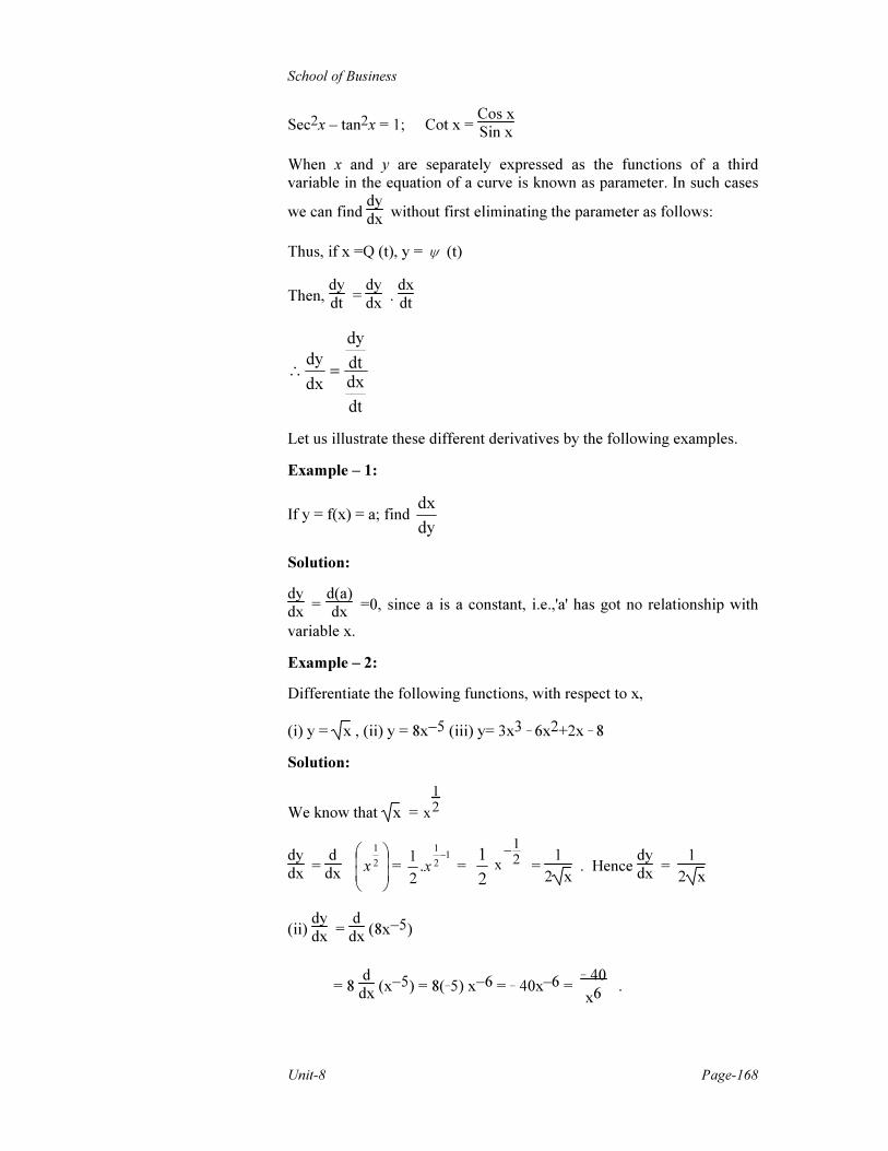
Sec2x – tan2x = 1; Cot x = Cos x

Sin x

When x and y are separately expressed as the functions of a third variable in the equation of a curve is known as parameter. In such cases

we can find dy

dx without first eliminating the parameter as follows:

Thus, if x =Q (t), y = ψ (t)

Then, dy

dt = dy

dx . dx

dt

dt

dxdt

dy

dx

dy=∴

Let us illustrate these different derivatives by the following examples.

Example – 1:

If y = f(x) = a; find dy

dx

Solution:

dy

dx = d(a)

dx =0, since a is a constant, i.e.,'a' has got no relationship with

variable x.

Example – 2:

Differentiate the following functions, with respect to x,

(i) y = x , (ii) y = 8x−5 (iii) y= 3x3 − 6x2+2x − 8

Solution:

We know that x = x

1

2

dy

dx =

d

dx

2

1

x = 1

2

1

.2

1 −

x = 2

1 2

1

x

−

= 1

2 x . Hence

dy

dx =

1

2 x

(ii) dy

dx =

d

dx (8x−5)

= 8 d

dx (x−5) = 8(−5) x−6 = − 40x–6 =

− 40

x6 .



Therefore, dy

dx =

− 40

x6

(iii) dy

dx =

d

dx (3x3 − 6x2+2x − 8)

= d

dx (3x3) −

d

dx (6x2) +

d

dx (2x) −

d

dx (8)

= 3.3x3−1− 2.6.x2−1+ 2−0 = 9x2

−12x+2

Thus, dy

dx = 9x2 − 12x + 2.

Example –3:

Differentiate ex(log x) . (2x2+3) with respect to x.

Solution:

Let y = ex.(log x) . (2x2 + 3)

dy

dx =ex (log x)

d

dx (2x2+3) +ex(2x2+3).

d

dx (logx) + (log x). (2x2 +3).

d

dx (ex)

=ex(logx)(4x)+ex(2x2+3)1

x + logx(2x2+3)ex

= ex[4x.logx + 2x2+3

x + (2x2 +3) logx]

So, dy

dx = ex[4x.logx +

2x2+3

x + (2x2 +3) logx]

Example–4:

If y = 2+3log x

x2+5 , find

dy

dx

Solution:

y = 2+3log x

x2+5

dx

dy=

22

22

)5(

)5()log32()log32()5(

+

++−++

x

xdx

dxx

dx

dx

=

(x2+5) (3

x)–(2+3logx)(2x)

(x2+5)2 =

15

x –x –6xlogx

(x2+5)2 .Thus,

dy

dx =

15

x –x –6xlogx

(x2+5)2

School of Business

Unit-8 Page-170

Example–5:

Find the differential co-efficient of 7x5x

2

e++

with respect to x.

Solution:

Let y= ex2+5x+y

dy

dx =

yx5x2

e++

. d

dx (x2 +5x +y) = e

x2 + 5x + y.

(2x + 5)

dy

dx = (2x + 5). ex

2

+ 5x + y

Example–6:

Find dy

dx , if y = log 4x+3

Solution:

Let y = log 4x+3

= log (4x + 3)

12 =

1

2 log (4x +3)

dy

dx =

d

dx [ 1

2 log (4x +3)] =

1

2 .

1

4x+3 . d

dx (4x +3) =

1

2 .

1

4x+3 . 4 =

2

4x+3

∴ dy

dx =

2

4x+3

Example–7:

Find the first, second and third derivatives when y = x.ex2

Solution:

y = x.ex2

First derivative,

dy

dx = x

d

dx ex

2 +ex

2. d

dx (x) = x.ex

2. 2x + ex

2.1 = ex

2 (2x2 +1)

Second derivative, d2y

dx2 = ex

2.2x(2x2+1) +ex

2.4x

= ex2. 4x3 +

2xe .2x + ex2

. 4x = ex2. (4x3 + 2x + 4x)

= ex2. (4x3 + 6x)



Third derivative,

d3y

dx3 = ex

2 2x (4x3 + 6x) + ex

2 (12x2 + 6)

= ex2. 8x4 +

2xe 12x2 + ex2

(12x2 + 6) = ex2 (8x4 + 12x2 + 12x2 + 6)

= ex2 (8x4 + 24x2 + 6)

Example–8:

If y = xlogx, find dy

dx

Solution:

Given, y = xlogx

Taking logarithm of both sides, we have

log y = log (xlogx) = logx. logx = (logx)2

Differentiating with respect to x, we get

1

y . dy

dx =

d

dx (logx) 2 =2 (logx)2-1

d

dx (logx) = 2 logx.

1

x

Hence, dy

dx = y (2 logx.

1

x ) =

2xlogx. logx

x

Example–9:

Find the derivative of log (ax + b) with respect to x.

Solution:

Let y = log (ax +b)

So, dy

dx =

d

dx [log (ax + b)] =

1

(ax+b) d

dx (ax + b) =

a

ax+b .

Therefore, dy

dx =

a

ax + b

Example–10:

Differentiate y = loga x with respect to x.

Solution:

We know that a

x

x

e

e

a

log

loglog =

School of Business

Unit-8 Page-172

So, ( )

==

a

x

dx

dx

dx

d

dx

dy

e

e

a

log

loglog

axxax

dx

d

aee

e

elog.

11.

log

1log.

log

1===

So, axdx

dy

elog.

1=

Example–11:

If y = xxx, find

dy

dx

Solution:

y = xxx

Taking logarithm of both sides, we have Let y = xx

log y = x

xxlog = xx log x. Then log y= x log x

Differentiating with respect to x, we get, d

dx(log y) = 1(log x) + x.

1

x

1

y .

dy

dx = xx

d

dx (log x) + log x

d

dx( xx ) = 1 + log x

or, 1

y .

dy

dx = xx .

1

x + log dxx (1+logx)

1

y

dy

dx = 1+ log x

∴

dy

dx = y [xx .

1

x + log xx (1+log x)] So,

dy

dx = y (1+log x)

= xxx [xx–1+ log xx (1+log x)] So,

dy

dx = xx (1+ log x)

Example–12:

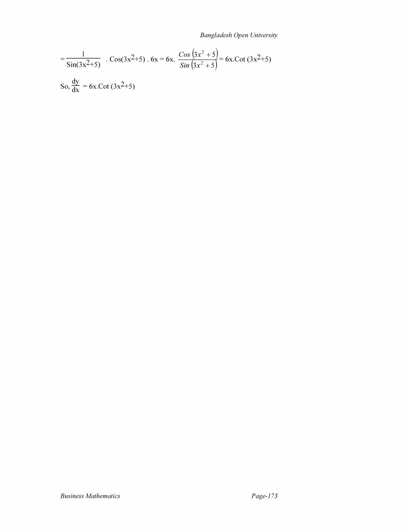
Differentiate y = log [Sin (3x2+5)] with respect to x.

Solution:

y = log [Sin (3x2+5)]

dy

dx =

d

dx [log {Sin (3x2+5)}]

= 1

Sin(3x2+5). d

dx [Sin (3x2+5)]

= 1

Sin(3x2+5) . Cos (3x2+5) .

d

dx (3x2+5)



= 1

Sin(3x2+5) . Cos(3x2+5) . 6x = 6x.

( )( )53

53

2

2

+

+

xSin

xCos= 6x.Cot (3x2+5)

So, dy

dx = 6x.Cot (3x2+5)

School of Business

Unit-8 Page-174

Questions for Review:

These questions are designed to help you assess how far you have understood and can apply the learning you have accomplished by answering (in written form) the following questions :

1. Define differentiation. What are the fundamental theorems of differentiation?

2. Why is the study of differentiation important in managerial decision making?

3. Find the derivative of the following functions with respect to x.

i) 5x4+3

x5 – 8x2+7x, (ii) (2x3–5x

–2+2) (4x2–3 x ) (iii) 5x2+9

3x–2

(iv) (3x2–2x+5)3/2 (v) 5exlogx, (vi) x2+3xy+y3=5 (vii) exx

4. If y=x3 log n, show that d4y

dx4 =6

x

5. Differentiate the following w. r. to x

(i) Sin x Cos x (ii) sin x

cos x (iii) e4x+log sin x

iv) (sin–1x)log x

6. If y = 8x3–5x3/2+3x2–7x+5 : find d3y

dx3

Multiple Choice Questions (√ the most appropriate answer)

1. Find dy

dx when y = log

2x

i) log2e (ii) 1

2 log2e (iii) 2log2e (iv) loge

2. Find the derivatives of the function 1+x

1–x

i) 2

1–x (ii)

1

(1–x)2 (iii)

2

(1–x)2 (iv) (1–x) 2

3. If f(x) = x3 – 2px2 – 4x + 5 and f (2) = 0, find p.

i) 1 (ii) 3 (iii) 4 (iv) 5



4. If f(x)=2x3–3x

2+4x–2, find the value of ( )2−=xf

dx

d

i) 30 (ii) 40 (iii) 25 (iv) 35

5. If f(x)= 2x – 2

x + x+4

4–x , find ( )2xf

dx

d=

i) 2.75 (ii) 2 (iii) 2.5 (iv) 2.45

6. Find the derivative of xx

i) xn(1+log n) (ii) x log n (iii) x2log n (iv) x2(1+log n)

7. If y = 8x3 – 5x3/2 + 3x2 – 7x +5. find d2y

dx2

i) 24x2 – 15

2 x 1/2+6x – 7 (ii) 48x –

15

2 x1/2+6

(iii) 48 + 15

8 x3 (iv) 48x –

15

2 x +7

School of Business

Unit-8 Page-176

Lesson-2: Differentiation of Multivariate Functions

Lesson Objectives:

After studying this lesson, you will be able to:

� State the nature of multivariate function;

� Explain the partial derivatives;

� Explain the higher- order derivatives of multivariate functions;

� Apply the techniques of multivariate function to solve the problems.

Introduction

The concept of the derivative extends directly to multivariate functions. During the discussion of differentiation, we defined the derivative of a function as the instantaneous rate of change of the function with respect to independent variable. In multivariate functions, there are more than one independent variable involved and thereby, the derivative of the function must be considered separately for each independent variable. For example, z = f (x, y) is defined as a function of two independent variables if there exists one and only one value of z in the range of f for each ordered pair of real number (x, y) in the domain of f. By convention, z is the dependent variable; x and y are the independent variables.

To measure the effect of a change in a single independent variable (x or y) on the dependent variable (z) in a multivariate function, the partial derivative is needed. The partial derivative of z with respect of 'x' measures the instantaneous rate of change of z with respect to x while y

is held constant. It is written dx

df

dx

dz, , fx (x, y), fx or Zx. The partial

derivative of z with respect to y measures the rate of change of z with

respect to y while x is held constant. It is written as: dy

df

dy

dz, , fy (x, y), fy

or Zy.

Mathematically it can be expressed in the following way:

( ) ( )x

yxfyxxf

dx

dz

x ∆

−∆+=

→∆

,,lim

0

( ) ( )y

yxfyyxf

dy

dz

x ∆

−∆+=

→∆

,,lim

0

Partial differentiation with respect to one of the independent variables follows the same rules as differentiation while the other independent variables are treated as constant.

This is illustrated by the following examples.

To measure the effect

of a change in a

single independent

variable (x or y) on

the dependent

variable (z) in a

multivariate function,

the partial derivative

is needed.



Example−1:

Find the partial derivatives of M = f (x, y, z) = x2+5y2+20xy+4z.

Solution:

To determine the partial derivative of f with respect to x, we treat y and z as constants.

dm

dx = fx´ = 2x + 20y.

Similarly, in determining the partial derivative of f with respect to y, we

treat x and z as a constants. dm

dy = fy´ = 10y + 20x

Finally, treating x and y as constants, we obtain the partial derivative of f

with respect to z dm

dz = fz´ = 4

The same procedure is applied in the following examples.

Example − 2:

Determine the partial derivatives of

Z = 5x3 −3x2y2 + 7y5

Solution:

dz

dx =

d

dx (5x3) −3y2

d

dx (x2) +

d

dx (7y5)

= 15x2−6xy2+0

∴ dz

dx = 15x2−6xy2

Again dz

dy =

d

dy (5x3) −3x2

d

dy (y2) +

d

dx (7y5)

= 0 − 6x2y + 35y4

∴dz

dy = 35y4 − 6x2y.

Example−3:

Find the partial derivatives of z = (5x + 3) (6x + 2y)

Solution:

dz

dx = (5x + 3).

d

dx (6x+2y) + (6x + 2y).

d

dx (5x+3)

= (5x +3). 6 + (6x +2y). 5

School of Business

Unit-8 Page-178

= 30x +18 +30x +10y

∴dz

dx = 60x +10y +18

Again dz

dy = (5x + 3).

d

dy (6x+2y) + (6x + 2y).

d

dx (5x+3)

= (5x + 3). 2 + (6x + 2y). 0

∴dz

dy = 10x + 6 + 0 = 10x + 6

Example−4:

Determine the partial derivatives of Z = 6x+7y

5x+3y

Solution:

dz

dx =

(5x+3y) d

dx (6x+7y) – (6x+7y)

d

dx (5x+3y)

(5x+3y)2

= (5x+3y). 6−(6x+7y).5

(5x+3y)2

dz

dx =

30x+18y−30x−35y

(5x+3y)2

∴ dz

dx =

−17y

(5x+3y)2

Again dz

dy =

(5x+3y). d

dy (6x+7y)−(6x+7y).

d

dy (5x+3y)

(5x+3y)2

= (5x+3y).7 − (6x+7y).3

(5x+3y)2

= 35x+21y−18x-21y

(5x+3y)2

∴

dz

dy =

17x

(5x+3y)2

Higher-Order derivatives of Multivariate Functions

The rules for determining higher-order derivatives of functions of one independent variable apply to multivariate functions. Derivatives of multivariate functions are taken with respect to one independent variable at a time, the remaining independent variables being considered as

Derivatives of multi-

variate functions are

taken with respect to

one independent

variable at a time.



constants. The same procedure applies in determining higher-order derivatives of multivariate functions.

For instance, a function f (x, y) may have four second-order partial derivatives as follows:

Original function First partial derivatives Second-order partial derivatives

xxf ′′ (x, y) or

d2f

dx dx or

2

2

dx

fd

yf ′′ (x, y) or

d(f)

dx

yxf ′′ (x, y) or

d2f

dy dx

f (x, y)

yf ′ (x, y) or

d(f)

dy

yxf ′′ (x, y) or

d2f

dx dy

yyf ′′ (x, y) or

d2f

dy dy or

2

2

dy

fd

The second-order partial derivatives xxf ′′ and

xyf ′′ are obtained by

differentiating xf ′′ , with respect to x and with respect to y respectively.

Similarly the second-order partial derivatives yxf ′′ and

yyf ′′ are obtained by

differentiating fy, with respect to x and with respect to y respectively.

The cross (or mixed) partial derivative xyf ′′ or

yxf ′′ indicates that first the

primitive function has been partially differentiated with respect to one independent variable and then that partial derivative has in turn been partially differentiated with respect to the other independent variable:

( ) yxxyff

′′=′′ =

d

dy

dz

dx =

d2z

dydx

( ) xyyzff

′′=′′ =

d

dx

dz

dy =

d2z

dxdy

The cross partial is a second-order derivative, which are equal always. That is

d2z

dydx =

d2z

dxdy

yxxyffor ′′=′′,


School of Business

Unit-8 Page-180

Example−5:

Determine (a) first, (b) second and (c) cross partial derivatives of Z =

7x3 + 9xy +2y5.

Solution:

(a) dz

dx = Zx = 21x

2 + 9y; dz

dy = Zy = 9x + 10y4.

(b) d2z

dx2 = Zxx = 42x;

d2z

dy2 = Zyy = 40y3.

(c) d2z

dydx =

d

dy .

dz

dx =

d

dy (21x2+9y) = Zxy = 9

d2z

dxdy =

d

dx .

dz

dy =

d

dx (9x+10y4) = Zyx = 9.

Example−6:

Determine all first and second-order derivatives of

Z = (x2+3y3)4

Solution:

dz

dx = 4 (x2+3y3)3. 2x = 8x (x2+3y3)3

dz

dy = 4 (x2+3y3)3. 9y2 = 36y2 (x2+3y3)3

d2z

dx2 = 8x[3(x2+3x3)2 (2x)] + (x2+3y3)3. 8

= 48x2 [x2+3x3]2 + 8(x2+3y3)3

d2z

dy2 = 36y2 [3(x2+3y3)2 (9y2)] + (x2+3y3)3 72y

d

2z

dydx =

d

dy .

dz

dx = 8x [3(x2+3y3)2 (9y2)]+0

= 216xy2 (x2+3y3)2

d2z

dxdy =

d

dx . dz

dy = 36y2 [3 (x2+3y3)2. 2x]

= 216xy2 (x2+3y3)2



Optimization of Multivariate Functions

For a multivariate function such as z = f (x, y) to be at a relative minimum or maximum, the following three conditions must be fullfiled /met:

1. Given z = f (x, y), determine the first-order partial derivatives, xf ′

(x, y) and yf ′ (x, y) and all critical point/values (a, b); that is,

determine all values (a, b) such that xf ′ (a, b) =

yf ′′ (a, b) = 0

2. Determine the second-order partial derivatives,

( ) ( ) ( )yxfyxfyxfyxxyxx

,,,,, ′′′′′′ and ( )yxfyy

,′′

[Note: the cross partial derivatives ( )yxfxy

,′′ (x, y) and ( )yxfy

,′′ (x, y) must be

equal to one another; otherwise the function is not continuous.]

3. Where (a, b) is a critical point on f, let D =xxf ′′ (a, b).

yyf ′′ (a, b) −

[xyf ′′ (a, b)]2

Then

(i) If D>0 and xxf ′′ (a, b) < 0, f has a relative maximum at (a, b)

(ii) If D>0 and xxf ′′ (a, b) > 0, f has a relative minimum at (a, b).

(iii) If D<0, f has neither a relative maximum nor a relative minimum at (a, b)

(iv) If D = 0, no conclusion can be drawn; further analysis is required.

This is illustrated by the following example.

Example−7:

Determine the critical points and specify whether the function had a relative maximum or minimum,

z = 2y3−x3+147x−54y+12.

Solution:

By taking the first-order partial derivatives, setting them equal to zero, and solving for x and y:

zx = −3x2 + 147 = 0 zy = 6y2−54=0

or, x2 = 49 or, 6y2 = 54

∴ x = + 7 ∴ y = + 3

School of Business

Unit-8 Page-182

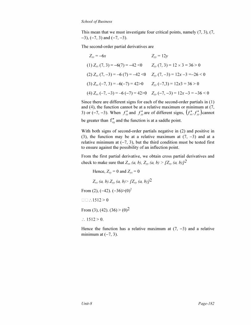
This mean that we must investigate four critical points, namely (7, 3), (7,

−3), (−7, 3) and (−7, −3).

The second-order partial derivatives are

Zxx = −6x Zyy = 12y

(1) Zxx (7, 3) = −6(7) = −42 <0 Zyy (7, 3) = 12 × 3 = 36 > 0

(2) Zxx (7, −3) = −6 (7) = −42 <0 Zyy (7, −3) = 12x −3 =−26 < 0

(3) Zxx (−7, 3) = –6(−7) = 42>0 Zyy (−7,3) = 12x3 = 36 > 0

(4) Zxx (–7, −3) = –6 (−7) = 42>0 Zyy (−7, −3) = 12x −3 = −36 < 0

Since there are different signs for each of the second-order partials in (1) and (4), the function cannot be at a relative maximum or minimum at (7,

3) or (−7, −3). When xyf ′′ and

yyf ′′ are of different signs, ( )

yyxxff ′′′′ . cannot

be greater than xyf ′′ and the function is at a saddle point.

With both signs of second-order partials negative in (2) and positive in

(3), the function may be at a relative maximum at (7, −3) and at a

relative minimum at (−7, 3), but the third condition must be tested first to ensure against the possibility of an inflection point.

From the first partial derivative, we obtain cross partial derivatives and

check to make sure that Zxx (a, b), Zyy (a, b) > [Zxy (a, b)]2

Hence, Zxy = 0 and Zyx = 0

Zxx (a, b).Zyy (a, b)> [Zxy (a, b)]2

From (2), (−42). (−36)>(0)2

JJ∴1512 > 0

From (3), (42). (36) > (0)2

∴ 1512 > 0.

Hence the function has a relative maximum at (7, −3) and a relative

minimum at (−7, 3).



Questions for Review

These questions are designed to help you assess how far you have understood and can apply the learning you have accomplished by answering (in written form) the following questions:

1. Determine first, second and cross − partial derivatives of

f (x, y) = 2x2 + 4xy2 − 5y2 + y3

2. Determine the first and second−order partial derivatives of the function

f (x, y, z) = x2ey In z.

3. Examine the function, z (x, y) = x2 + y2 − 4x + 6y for relative maxima or minima by using second- order derivative test.

4. Find the partial derivatives for z = (6x + 4) (4x + 2y)

School of Business

Unit-8 Page-184

Lesson-3: Optimization with Lagrangian Multipliers

and Cobb-Douglas Production Functions


� Discuss the nature of constrained optimization with lagrangian multipliers;

� Discuss the nature of optimization of Cobb-Douglas Production functions;

� Apply the techniques to solve the relevant problems.

Constrained Optimization with Lagrangian Multipliers

Differential calculus is also used to maximize or minimize a function subject to constraints. Given a function f (x, y) subject to a constraint g (x, y) = k (a constant), a new function F can be formed by– (1) setting the

constraint equal to zero, (2) multiplying it by λ (the lagrange multiplier), and (3) adding the product to the original function :

F (x, y, λ) = f (x, y) + λ [k−gcx, y)].

Here F (x, y, λ) = Lagrangian functions

f (x, y) = original or objective function

and g (x, y) = constraint.

Since the constraint is always set equal to zero, the product λ [k−g (x, y)] also equals zero, and the addition of the term does not change the value

of the objective function. Critical values x0, y

0 and λ0, at which the

function is optimised, are found by taking the partial derivatives of F with respect to all three independent variables, setting them equal to zero, and solving simultaneously:

Fx (x, y, λ) = 0 Fy (x, y, λ) =0; Fz (x, y, λ) = 0


Example–1:

Determine the critical points and optimise the function

Z = 4x2 + 3xy + 6y2 subject to the constraint x + y = 56.

Solution:

Setting the constraint equals to zero, 56 – x – y = 0

The lagrangian expression is,

F (x, y, λ) = Z = 4x2 + 3xy + 6y2 + λ(56 – x – y) ...(1)

and the partial derivatives are

Differential calculus

is also used to maxi-

mize or minimize a

function subject to

constraints.

Since the constraint is

always set equal to

zero, the product λ

[k−g (x, y)] also

equals zero.



d(F)

dx = Zx = 8x + 3y – λ= 0 ... (2)

d(F)

dy = Zy = 3x +12y – λ= 0 ... (3)

d(F)

dl = Zλ = 56 – x – y = 0 ... (4)

Subtracting (3) from (2) to eliminate λ gives

5x – 9y = 0

or 5x = 9y

∴x = 1.8y ... (5)

Substituting x = 1.8y in equation (4)

1.8y + y – 56 = 0

or, 2.8y = 56

∴ y = 56/2.8 = 20.

Substituting y = 20 in equation (5) we get

x = ( )208.1 × = 36

Substituting x = 36 and y = 20 in equation (2) we have

8 (36) + 3(20) – λ = 0

or, 288 + 60 – λ = 0

or, 348 – λ = 0

∴ λ = 348

Substituting the critical values, x = 36, y = 20 and λ = 348 in lagrangian function, we have,

Z = 4(36)2 + 3(36) (20) + 6(20)2 + 348(56 – 36 – 20)

= 4 (1296) + 3(720) + 6(400) + 348 (0) = 9744.

Example–2:

Use lagrange multipliers to optimize the function, f (x, y) = 26x–3x2 +

5xy – 6y2 + 12y subject to the constraint 3x + y = 170.

Solution:

The lagrangian function is

F = 26x–3x2+5xy–6y2+12y+λ (170–3x–y) ... (1)

School of Business

Unit-8 Page-186

Thus Fx = 26–6x + 5y – 3λ = 0 ... (2)

Fy = 5x–12y +12–λ = 0 ... (3)

Fλ = 170 – 3x – y = 0 ... (4)

Multiplying equation (3) by 3 and subtracting from equation (2) to

eliminate λ, we have

–21x + 41y – 10 = 0 ... (5)

Multiplying equation (4) by 7 and subtracting from equation (5) to eliminate x, we have

48y – 1200 = 0

∴ 48y = 1200

∴ y = 25

Substituting y=25 in equation (4), we get

170 – 3x – 25 = 0

or, –3x = –145

∴ x = 4813

Then substituting x = 4813 and y = 25 in equation (2), we get λ = – 46

13

Using x0 = 4813 , y = 25 and λ = – 46

13 in lagrangian expression, we get

F=26

4813 –3

4813 2+5

4813 (25) –6(25)

2+12(25)+

170–3

4813 –25

∴ F = – 3160

Example–3:

Determine the critical points and the constrained optima for Z = x2 + 3xy

+ y2 subject to x + y = 100

Solution:

The lagrangian expression is F (x, y, λ) = f (x, y) + λ. g (x, y)

= x2 + 3xy + y2+λ (x + y –100)

and the partial derivatives are

dF

dx = 2x + 3y + λ = 0



dF

dy = 3x + 2y + λ = 0

λd

dF = x + y – 100 = 0

The three equations are solved simultaneously to obtain x = 50, y = 50

and λ = 250.

The critical values of x, y and λ can be substituted into the lagrangian expression to obtain the constrained optimum.

F (50, 50, –250) = (50)2+3(50) (50)+(50)2–250 (50+50–100)

= 2500 + 7500 + 2500 – 0 = 12,500.

To determine whether the function reaches a maximum or a minimum, we evaluate the function at points adjacent to x = 50 and y = 50. The

function is a constrained maximum, since adding ∆x and ∆y to the function in both directions gives a functional value less than the constrained optimum, i.e.

F (49, 51, – 250) = 12499

F (51, 49, – 250) = 12,499

Optimization of Cobb-Douglas Production Functions

Economic analysis is frequently couched in terms of the Cobb-Douglas

production function, Q = AKαLβ (A>0; 0<α, β<1) where Q is the quantity of output in physical units, K the quantity of capital, and L the

quantity of labor. Here α (the output elasticity of capital) measures the percentage change in Q for a 1 percent change in K while L is held

constant; β (the output elasticity of labor) is exactly parallel; and A is an efficiency parameter reflecting the level of technology.

A strict cobb-douglas function, in which α + β = 1, shows constant

returns to scale and decreasing returns to scale if α+β <1. A cobb-douglas function is optimized subject to a budget constraint. This is illustrated by the following examples.

Example–4:

Optimize the Cobb-Douglas production function, Q = k0.4 L0.5, given Pk = 3, PL= 4 and B = 108.

Solution:

By setting up the lagrangian function, we get

Q = k0.4 L0.5 λ (108 – 3k – 4L)

A strict cobb-douglas

function, in which α +

= 1, shows constant

returns to scale and

decreasing returns to

scale if α+β <1.

School of Business

Unit-8 Page-188

Using the simple power function rule, taking the first-order partial derivatives, setting them equal to zero and solving simultaneously for K0

and L0 (and λ0, if desired)

d(Q)dk = Qk = 0.4K

–0.6. L0.5 – 3λ = 0 ... (1)

dQdL = QL = 0.5K

0.4. L–0.5 – 4λ=0 ... (2)

dQdl = 108–3k–4L = 0 ... (3)

Rearranging, then dividing (1) by (2) to eliminate λ, we get.

5.04.0

056.0

.5.0

.4.0

−

−

LK

LK

or, .8k–1L1 = 0.75

or, LK =

0.750.8

∴L = 0.9375k.

Substituting L = 0.9375k in equation (3), we get

108–3k–4 (0.9375k) =0

∴Ko=16.

Then by substituting Ko=16 in equation (3), we have

108–3 (16)–4L = 0

or, 108–48–4L=0

or, – 4L = –60

∴ L0=15

Example–5:

From the following information find least cost input combination and the minimum cost of production:

Qn = 500, Pd = Tk.10 and Pk = Tk.0.50. Subject to Qn = 1.01 L0.75. K.0.25

Solution:

It can be stated that minimize,

C = 10L + 0.50K

Subject to 500 = 1.01L0.75 K0.25



Where, A. b, a are positive constants, a +b=1

b = 0.75; a = 0.25; A = 1.01

This can be solved through the lagrangian multiplier technique. The lagrangian expression would be

V = LPL + KPK + λ J[Q – ALb Ka ]

or, V = 10L + 0.50K + λ [500 – 1.01 L0.75 K0.25]

Where λ is the lagrangian multiplier, and V is the minimum cost.

The necessary condition for optimization is that each of the partial derivatives of V with respect to L And K must be equal to zero.

dVdL or V'(L) = 10– λ [1.01(0.75) L

–0.25 K0.25] = 0

So, λJ= 25.025.0

K.L7575.0

10

−

----------- (L)

d(V)dK or V'(K) = 0.50 – λ [1.01 L

0.75(0.25)K–0.75] = 0

∴ 0.50 – λ [0.2525 L0.75 K –0.75] = 0

So, λJ = 75.075.0

.2525.0

50.0

−

KL

---- -----(K)

We know that

Then we get,

50.0

10

2525.0

7575.0

75.075.0

25.025.0

=−

−

KL

KL

or, 3KL =

100.50

or, 1.5K = 10L

So, K = 5.1

L10 ∴K = 6.67L

Substituting the value of K in the original subject to the production function, we have

500 = 1.01 ( ) 25.075.067.6 LL

Marginal physical product of labor (MPPL) PL = Marginal physical product of capital (MPPK) PK

School of Business

Unit-8 Page-190

Taking logarithm of both sides, we get

log 500 = log1.01+0.75logL+0.25log(6.67)+0.25log L

or, log 500 – log 1.01 = log L + 0.25log(6.67)

or, 2.69897 – 0.00432 = log L + 0.25(0.82413)

or, log L = 2.48862

So, L = anti-log 2.48862 = 308.05 = 309 units (app),

Substituting the value of L, we have

K = 6.67 L

= 6.6 (308.7) = 2054.69 units (app) rounded to = 2055 Units

Substituting the value of L and K, we have,

C = 10L + 0.50K = 10 (309) + 0.50 (2055) = 3090 + 1027.50

= Tk.4117.50

Hence the least cost input combination is L = 309 and K = 2055 units and the minimum cost of production is Tk.4117.50



Questions for Review

These questions are designed to help you assess how far you have

understood and can apply the learning you have accomplished by

answering (in written form) the following questions:

1. Defermine the critical points and optimize the function

f(x, y)=5x2+6xy–3y2+10 subject to the constraint x+2y=24.

2. Find the maxima and minima of the following function subject to

the constraining equation.

f (x, y)=12xy – 3y2 – x2 and x + y = 16.

3. Optimize the following Cobb-Douglas production functions

subject to the given constraint. Q = K0.3L0.5 subject to 6K + 2L =

384.

4. Optimize the following Cobb-Douglas production function subject

to given constraints by Q = 10k0.7×L0.1 given Pk = 28, PL = 10

and β = 4000.

School of Business

Unit-8 Page-192

Lesson-4: Business Applications of Differentiation

Lesson Objectives:


� State the key concepts related to business applications of differentiation;

� Apply the techniques of differentiation to solve business problems.

Key Concepts

Total costs (TC): Total cost is the combination of fixed cost and variable cost of output. If the production increases, only total variable cost will increase in direct proportion but the fixed cost will remain unchanged within a relevant range.

Total revenue (TR): Total revenue is the product of price/demand function and output.

Profit: Profits are defined as the excess of total revenue over total costs. Symbolically it can be expressed as, P (profit) = TR – TC. i.e., (Total Revenue – Total Cost)

The rules for finding a maximum point tell us that P is maximized when the derivative of the profit function is equal to zero and the second derivative is negative. If we denote the derivatives of the revenue and cost functions by dTR and dTC we have,

'P' is at a maximum when dTR - dTC = 0. This equation may be written as dTR = dTC.

The derivative of the total revenue function must be equal to the derivative of the total cost function for profits to be maximized.

Profit Maximizing output = d(profit function)

dx

Condition: In case of maximization, the conditions are dp

dx = 0 and

d2p

dx2

must be Negative.

Cost Minimizing output = d(total cost function)

dx

Condition: In case of minimization, the conditions are dTCy

dx = 0 and

d2TC

dx2 must be Positive.

Marginal Cost (MC): MC is the extra cost for producing one additional unit when the total cost at certain level of output is known. Hence, it is

The rules for finding a

maximum point tell us

that P is maximized

when the derivative of

the profit function is

equal to zero and the

second derivative is

negative.



the rate of change in total cost with respect to the level of output at the

point where total cost is known. Therefore, we have, MC = dTC

dx where

total cost (TC) is a function of x, the level of output.

Marginal Production (MP): MP is the incre–mental production, i.e., the

additional production added to the total production, i.e. MP = dTP

dx

Marginal Revenue (MR): MR is defined as the change in the total revenue for the sale of an extra unit. Hence, it is the rate of change total in revenue with respect to the quantity demanded at the point where total

revenue is known. Therefore, we have, MR = dTR

dx where total revenue

(TR) is a function of x, the quantity demanded.

Let us illustrate these concepts by the following examples.

Example–1:

The profit function of a company can be represented by P =f (x) = x –

0.00001x2, where x is units sold. Find the optimal sales volume and the amount of profit to be expected at that volume.

Solution:

The necessary condition for the optimal sales volume is that the first derivative of the profit function is equal to zero and the second derivative must be negative. Where the profit function is:

P = x – 0.00001x2

( )200001.0 xxdx

d

dx

dP−=

Marginal Profit = 1 – 0.00002x

To get maximum profit now we put marginal profit = 0

So, 1 – 0.00002x = 0

or, 0.00002x = 1

So, x = 0.00002 = 50,000 units.

The second derivative of profit function, i.e.

d2P

dx2 = ( ) 000002.000002.01 <−=− x

dx

d

Now by putting the value of x in profit function we get maximum profit.

P = x – 0.00001x2

= 50,000 – 0.00001(50,000)2 = 50,000 – 0.00001(2500000000)

MR is defined as the

change in the total

revenue for the sale of

an extra unit.

School of Business

Unit-8 Page-194

= 50,000 – 25,000 = 25,000.

The optimum output for the company will be 50,000 units of x and maximum profit at that volume will be Tk.25,000.

Example – 2:

If the total manufacturing cost 'y' (in Tk.) of making x units of a product is : y = 20x + 5000, (a) What is the variable cost per unit? (b) What is the fixed cost? (c) What is the total cost of manufacturing 4000 units? (d) What is the marginal cost of producing 2000 units?

Solution:

We have the cost-output equation : y = 20x + 5000. We know that, if the production increases, only total variable cost will increase in direct proportion but the fixed cost will remain unchanged in total. So, the derivative of y with respect to the increase in x by 1 unit will give the variable cost per unit.

(a) Variable cost per unit = ddx (cost-output equation)

= ddx (y)

= ddx (20x + 5000) = 20.

∴ Variable cost per unit is Tk.20.

(b) Total fixed cost will remain unchanged even if we don't produce any unit. If we don't produce any unit, there will be no variable cost and only fixed cost will be the total cost. So, if we put x=0 in the cost-output equation, we will get the fixed cost.

∴ Fixed Cost = y = [20.(0) + 5,000] = Tk.5000

(c) If we put x=4000 in the cost-output equation, we will get the total cost of producing 4,000 units.

∴ Total cost of producing 4000 units = y = 20 (4,000) + 5,000 = Tk.85,000.

(d) We know that the marginal cost of 'n'th unit = TCn–TCn–1

∴ Marginal cost of 2000th unit

= TC of 2000 units – TC of (2000–1) units

= [20 (2000) + 5000] – [20 (1999 Tk. + 5000] = [45,000 – 44,980] = 20.

Example–3:



The total cost of producing x articles is 54 x

2 + 175x + 125 and the price

at which each article can be sold is 250 – 54 x. What should be the output

for a maximum profit. Calculate the profit.

Solution:

Total revenue (TR) =

− xx4

5250 = 250 –

5x2

2

Total cost (TC) = 5x2

4 + 175x +125

So, profit (P) = TR – TC

= 250x – 5x2

2 –

5x2

4 – 175x -125 =

–10x2–5x2 4

+ 75x –125 = –15x2

4 + 75x -125

d(p)dx =

–30x4 +75

The necessary condition for optimization is that the first derivative of a profit function is equal to zero and second derivative must be negative. According to the assumption, we have

–30x4 + 75 = 0

or, –30x + 300

4 = 0

or, –30x +300 = 0

or, –30x = –300

or, x = 10

and 04

3075

4

30.

2

2

<−

=

+

−==

x

dx

d

dx

dp

dx

d

dx

pd

Therefore the profit is maximum when the output (x) is 10

Profit function = –15x2

4 + 75(x) – 125

Putting the value of x in profit function, we get,

Profit = –15(10)2

4 + 75(10) – 125

= –15004 +750 – 125 = –375 +750 – 125 = 750 – 500 = 250

School of Business

Unit-8 Page-196

Hence the profit is Tk. 250.

Example–4:

The total cost function of a firm is C= 13 x

3 – 5x2 + 28x +10, where C is

total cost and x is output. A tax at the rate of Tk.2 per unit of output is imposed and the producer adds it to his cost. If the market demand function is given by P = 2530 – 5x, where P is the price per unit of output, find the profit maximizing output and price.

Solution:

Total Revenue (TR) = (2530 – 5x) x = 2530x – 5x2

Total cost (TC) = (13 x

3 – 5x2+28x + 10) + (Taxes i.e.2x)

= 13 x

3 – 5x2 + 28x + 10 + 2x = 13 x

3 – 5x2 + 30x + 10

So, profit (P) = TR –TC

= 2530x – 5x2 – 13 x3 + 5x2 – 30x – 10 = 2500x –

13 x

3 – 10.

So, d(P)dx = 2500 –

3x2

3 = 2500 – x2

The necessary condition for maximization is that the first derivative of a profit function is equal to zero and second derivative must be negative.

According to the condition, we can write

2500 – x2 = 0

or, – x2 = – 2500

So, x = 50

and 2

2

dx

pd= – 2x = – 2x 50 = –100 < 0

Hence the profit maximizing output of the firm is 50 units.

At this level, the price is given by

Price = 2530 – 5x = 2530 – 5 × 50 = 2530 – 250 = Tk.2280.

Example–5:

A motorist has to pay an annual road tax of $50 and $110 for insurance. His car does 30 miles to the gallon which costs 75 Pence (per gallon). The car is serviced every 3000 miles at a cost of $20, and depreciation is calculated in pence by multiplying the square of the mileage by 0.001.



Obtain an expression for the total annual cost. Hence find an expression for the average total cost per mile and calculate the annual mileage which will minimize the average cost per mile.

Solution:

Suppose he covers x miles in a year.

Tax per annum = $50; Insurance per annum $ 110

Cost of petrol =30

x75.; Service charges =

20x3000 .20

Depreciation = 0.001x2

100 (0.001 is in pence and is divided by 100 to get $ amount)

Total cost: C = 50+1102

x00001.03000

x20

30

x75.0++

Average TC per mile: Cx = M =

160x +

0.7530 +

203000 +0.00001x

dMdx =

ddx 160 x

–1 + 0.7530 +

203000 + 0.00001x

= –160 x–2 + 0 + 0 + 0.00001

= 00001.0160

2+−

x

The necessary condition for minimization of cost is dMdx = 0, and

d2M

dx2

must be positive.

According to the condition, we can write –160

x2 + 0.00001 = 0

or, 160

x2 = 0.00001

or, 0.00001x2 = 160

or, x2 = 160

0.00001 = 16000000

or, x = 4000

The average cost is a minimum since d2M

dx2 = –160 x–2 + 0.00001

= 320 x–3 + 0 = 320

x3 > 0

School of Business

Unit-8 Page-198

So, the motorist can cover 4000 miles in a year to minimize the average cost per mile.

Example–6:

The yearly profits of ABC company are dependent upon the number of workers (x) and the number of units of advertising (y), according to the function

P(x,y) = 412 x + 806y–x2–4y2–xy–50,000

(i) Determine the number of workers and the number of units in advertising that results in maximum profit.

(ii) Determine maximum profit.

Solution:

(i) To determine the values of x and y, we equate the partial derivatives of the profit function with zero.

Px (x, y) = 412–2x-y = 0 ... (1)

Py (x, y) = 806–x–8y = 0 ... (2)

The two equation are solved simultaneously to obtain the values of x and y.

412 – 2x – y = 0

1612–2x–16y = 0 ----------------------- – 1200 +15y = 0

or, 15y=1200

∴ y = 80

Substituting the value of y in equation (1), we get

412–2x–80=0

or – 2x = –332

∴x = 166

and

Pxx (x, y) = –2<0

Pyx (x, y) = –8 <0

(ii) The profit generated from using these values is:

P (166, 80) = 412 (166)+806 (80) – (166)2 – 4 (80)2– (166) (80) –50000



= 68392 + 64640 – 27556 –25600 – 13280– 50,000

=16595

Example – 7:

The cost of construction (c) of a project depends upon the number of skilled workers (x) and unskilled workers (y). If cost is given by, C (x, y)

= 50000+9x3–72xy+9y2

(i) Determine the number of skilled workers and unskilled workers that results in minimum cost.

(ii) Determine the minimum cost.

Solution:

To determine the number of skilled workers (x) and unskilled workers (y), we equate the partial derivatives of the cost function with zero.

Cx (x, y) = 27x2–72y = 0 ... (1)

Cy (x, y) = –72x + 18y = 0 ... (2)

Solving the two equations simultaneously gives

27x2 – 72y = 0

–288x + 72y = 0 [Multiplying equation (2) by 4] ---------------------------

By adding 27x2 – 288x = 0

or, x (27x – 288) = 0

or, 27x – 288 = 0

or, 27x = 288

∴ x = 10.66 rounded to

Substituting x = 11 in equation (2) we get

–72 (11) + 18y = 0

or, –792 +18y = 0

or, 18y = 792

∴ y = 79218 = 44

(ii) Putting the value of x and y in cost function, we get:

C (11, 44) = 50000 + 9 (11)3–72 (11) (44) + 9 (44)2

= 44,555

School of Business

Unit-8 Page-200

Questions for Review:

These questions are designed to help you assess how far you have

understood and can apply the learning you have accomplished by

answering (in written form) the following questions:

1. A study has shown that the cost of producing sign pens of a

manufacturing concern is given by, C = 30 + 1.5x + 0.0008x2.

What is the marginal cost at x = 1000 units? If the pens sells for

Tk.5.00 each, for what values of x does marginal cost equal

marginal revenue?

2. The demand function faced by a firm is P=500 – 0.2x and its cost

function is C=25x+10,000. Find the optimal output at which the

profits of the firm and maximum. Also find the price it will

charge.

3. The demand function of a profit maximizing monopolist is, P–3Q–

30 = 0 and his cost function is, C = 2Q2+10Q. If a tax of taka 5 per

unit of quantity produced is imposed on the monopolist, calculate

the maximum tax revenue obtained by the Government.

4. A company produces two products, x units of type –A and y units

of type –B per month. If the revenue and cost equation for the

month are given by-

R (x, y) = 11x +14y, C (x, y) = x2 – xy +2y2 + 3x + 4y +10

5. Total cost function is given by, TC = 3Q2+7Q+12, Where C=Cost

of production, Q = output. Find

(i) marginal cost

(ii) Average cost if Q = 50

6. The total cost of production for the electronic module

manufactured by ABC Electronics is

TC = 0.04Q3 – 0.30Q2 + 2Q + 1

7. Determine MC, AC, AFC and TVC function. Find out the output

level for which MC is minimum. What is the amount of MC, AC

and TC at this level of output.

8. The transport authority of the city corporation areas has

experimented with the fare structure for the city’s public bus

system. The new system is fixed fare system in which a passenger

may travel between two points in the city for the same fare. From

the survey results, system analysis have determined an appropriate

demand function, P=2000–125Q, where Q equals to the average

number of riders per hours and p equals the fare in taka.

Required:



(i) Determine the fare which should be charged in order to

maximize hourly bus for revenue.

(ii) How many rider are expected per hour under this fare?

(iii) What is the expected maximum annual revenue?

differentiation and its uses in business problems 8

Documents