Contents lists available at ScienceDirect

Optics Communications

journal homepage: www.elsevier.com/locate/optcom

Diffraction of a Gaussian beam by a four-sector binary grating with a shiftbetween adjacent sectors

Lj. Janicijevica, S. Topuzoskia,⁎, L. Stoyanovb, A. Dreischuhb

a Faculty of Natural Sciences and Mathematics, Institute of Physics, University “Ss. Cyril and Methodius”, Skopje 1000, Republic of Macedoniab Department of Quantum Electronics, Faculty of Physics, Sofia University “St. Kliment Ohridski”, Sofia 1164, Bulgaria

A R T I C L E I N F O

Keywords:DiffractionDiffractive optical elementGaussian laser beamFour-sector binary grating

A B S T R A C T

In this article as a diffractive optical element we consider a composed four-sector binary grating under Gaussianlaser beam illumination. The angular sectors are bounded by the directions y x= and y x= − , and consist ofparts of a binary rectilinear grating; thereby, two neighboring parts are shifted by a half spatial rectilineargrating period. The diffracted wave field amplitude is calculated, showing that the straight-through, zeroth-diffraction-order beam is an amplitude-reduced Gaussian beam, and the higher-diffraction-order beams,deviated with respect to the propagation axis, are non-vortex beams described by modified Bessel functions. Thetransverse intensity profiles of the higher-diffraction-order beams, numerically and experimentally obtained,have form of a four-leaf clover; they are similar to the Laguerre-Gaussian LG(0,2) beam (with radial modenumber n = 0 and azimuthal mode number l = 2) described by circular cosine function, in a paraxial, far-fieldapproximation.

1. Introduction

Besides the fundamental mode (Gaussian beam), the Hermite–Gaussian (HG) and Laguerre–Gaussian (LG) beams are also solutionsof the paraxial wave equation [1]. Lot of research has been done toanalyze their theoretical and experimental properties, and to investi-gate their applications in the basic optical sciences and in otherscientific fields (see e.g. Ref. 2 and references therein). Linearlypolarized LG beams with nonzero azimuthal mode number are carriersof screw dislocations and possess orbital angular momentum (OAM)[3]. They are optical vortex beams. In the field of singular optics themostly used are LG beams with zero radial mode number. The family ofLG beams covers the cases of the equiaxial linear combinations(addition or subtraction) of two LG beams with equal azimuthal modenumber value l, but with opposite signs of l (opposite orientations oftheir OAMs), as well. As a result, the two coupled vortex beams create abeam without OAM (no topological charge), possessing profiles de-scribed by circular functions lφcos( ) or lφsin( ).

The linearly polarized HG(m,n) beams have degenerate edgedislocations in their wavefronts and do not possess OAM [3].

Nye and Berry have described, classified and analyzed the wave-fronts defects in wave trains and monochromatic waves [4]. In laserbeams having structure of transverse cavity modes, edge dislocationsoccur as black lines between π-shifted in phase mode spots; the

simplest is the TEM01, where the zeroth-value intensity line dividesthe beam into two parts corresponding to phase shift of π. In [5] theauthors showed that, an edge dislocation of the wavefront can beproduced experimentally by using two binary periodic gratings, shiftedby half a period on a line of zero amplitude. Then, in the process ofdiffraction, the incident Gaussian laser beam is divided with a dark lineinto two bright spots. Whereas, a binary fork-shaped grating with anedge dislocation in direction θ = 0 produces mixed screw-edge disloca-tion, as shown experimentally in [5].

The vortex beams are created in laser resonators, or by usingdiffractive optical elements which transform the Gaussian beam into avortex one, such as spiral phase plate [6–8], helical axicon [9–12],helical lens [13], computer-generated holograms [14,15], fork-shapedgratings [16,17] etc. The computer-generated gratings (CGGs) accom-panied with the photo-reduction methods have an advantage over theexpensive lithographic methods. Except the simple, fast and cheapproduction, they make possible the creation of combined gratings,which can substitute the laser resonators in making new interestinglaser modes. Liquid crystal spatial light modulators make this proce-dure even more flexible ensuring high efficiency and fast reconfigura-tion.

In this article we consider a CGG constructed by inserting parts of abinary rectilinear grating into the four equal angular sectors, boundedby the directions y x= and y x= − (Fig. 1). Thus, two neighboring parts

http://dx.doi.org/10.1016/j.optcom.2016.12.041Received 20 November 2016; Received in revised form 14 December 2016; Accepted 18 December 2016

⁎ Corresponding author.E-mail address: suzana_topuzoski@yahoo.com (S. Topuzoski).

Optics Communications 389 (2017) 203–211

Available online 27 December 20160030-4018/ © 2016 Elsevier B.V. All rights reserved.

MARK

of the grating are shifted by a half spatial grating period along x axis.We analytically calculate the diffraction pattern obtained by illuminat-ing the grating with a Gaussian laser beam, which enters into thegrating plane with its waist and intersects the grating plane centre withits axis. The far-field diffraction patterns of the higher-diffraction-order(HDO) beams, in a paraxial approximation are similar to Hermite-Gaussian HG(1,1) or cosine-LG(n=0,l=2) laser mode: four bright spotsare nested in four quadrants divided by crossed one-dimensional phasedislocations. With this method we create in the HDOs beams withcoupled optical vortices [18] and crossed dark lines, which are ofinterest for many applications as optical trapping, optical communica-tion, angular alignment etc.

2. Construction and transmission function of the grating

The computer generation of this grating consists in inserting partsof a binary rectilinear grating into the four equal angular sectors,bounded by the directions y x= and y x= − . The area of each of thesectors, numbered by n=(1), (2), (3) and (4), is successively covered bya negative (in (1) and (3)) and positive (in (2) and (4)) gratings, bothpossessing the same period d ξ= 2 0 (Fig. 1). In a rectangular coordinatesystem, whose ordinate is the axis of symmetry of both types ofgratings, their transmission functions are expressed by the cosineFourier series as

∑t x m π m πξ

x( ) = 12

± sinc (2 − 1)2

cos (2 − 1) .gm

±

=1

∞

0

⎛⎝⎜

⎞⎠⎟

⎛⎝⎜

⎞⎠⎟ (1)

Since we will treat the problem of diffraction of a Gaussian laserbeam by the computer-generated gratings in cylindrical coordinatesystem, we will use the polar coordinates r φ( , ) for the grating's plane.The pole is situated in the intersection point of the y x= and y x= −lines. Then, the transmission functions t r φ( , )g

+ for the positive (withwhite central line) and t r φ( , )g

− for the negative (with dark central line)gratings, are defined as

∑t r φ m π i m πξ

r φ

i m πξ

r φ

( , ) = 12

± 12

sinc (2 − 1)2

exp + (2 − 1) cos

+ exp − (2 − 1) cos .

gm

±

=1

∞

0

0

⎛⎝⎜

⎞⎠⎟

⎡⎣⎢

⎛⎝⎜

⎞⎠⎟

⎛⎝⎜

⎞⎠⎟

⎤⎦⎥ (2)

In Eq. (1) and Eq. (2) the transmission coefficients arem π π msinc((2 − 1) /2) = 2(−1) /( (2 − 1))m( −1) m( = 1, 2, 3, ... ), while the

sign “+” in front of the sum stands for the positive grating.As it is seen in Fig. 1, the n-th quadrant is occupied by one of the

upper mentioned gratings. Each of them is an angular sector of π/2 rad, which in absence of the grating, is a completely transparentaperture between the directions φ n π= (2 − 1) /4 and φ n π= (2 + 1) /4.Using the Heaviside unite step function E φ φ φ φ φ π( − ) = 1 >

0 otherwise(0 < < 2 )0

0⎧⎨⎩ ,

we define the n-th sector aperture transmission function as

t φ E φ n π E φ n π

n π φ n π n

( ) = ( − (2 − 1) /4) − ( − (2 + 1) /4)

= 1 (2 − 1) /4 < < (2 + 1) /40 otherwise

( = 1, 2, 3, 4)

an( )

⎧⎨⎩ (3)

The transmission function of the composed grating in Fig. 1 is asum of the four sector transmission functions t r φ t φ t r φ( , ) = ( ) ( , )a

ng

( ) ±

(for n=1,2,3,4) and is defined by

t r φ E φ n π E φ n π

m m r φ

( , ) = ∑ { ( − (2 − 1) /4) − ( − (2 + 1) /4)}

× + (−1) ∑ sinc (2 − 1) cos (2 − 1) cos .

n

nm

π πξ

=14

12 =1

∞2 0

⎪

⎪

⎪

⎪

⎧⎨⎩

⎛⎝⎜

⎞⎠⎟

⎛⎝⎜

⎞⎠⎟

⎫⎬⎭(4)

The grating whose transmission function is given by expression Eq.(4) will be used as an optical diffracting device in our further investigation.

3. Diffraction of a Gaussian laser beam by the composedfour-sector grating

The Gaussian beam is normally incident on the plane of the grating,with its propagation axis (z axis of the cylindrical coordinate system)passing through its centre, and its waist located in the plane of thegrating. Thus, the incident beam is defined by:U r φ z r w ikr q( , , = 0) = exp(− / ) = exp(− /2 (0))i 2

02 2 where w0 is the beam

waist radius, k π λ= 2 / is the propagation constant and q (0) is the beamcomplex parameter in the waist plane. If the grating is absent, atdistance z from the origin the beam has a complex parameterq z z ikw( ) = + /20

2 , with q ikw iz(0) = /2 =02

0, and z0 being the beamRayleigh distance. The field of the diffracted light is defined by theFresnel-Kirchhoff integral

∫ ∫U ρ θ z ikπz

ik z ρz

t r φ U r φ

ikz

r rρ φ θ r r φ

( , , ) =2

exp − +2

( , ) ( , )

× exp −2

( − 2 cos( − )) d d .

πi

2

0

∞

0

2( )

2

⎡⎣⎢

⎛⎝⎜

⎞⎠⎟

⎤⎦⎥

⎡⎣⎢

⎤⎦⎥ (5)

The polar coordinates ρ θ( , ) characterize the observation plane Πsituated at distance z from the grating. Substitution of the incidentbeam and the transmission function Eq. (4) in the diffraction integralgives

∑ ∑U ρ θ z U ρ θ z U ρ θ z

U ρ θ z

( , , ) = ( , , ) + ( ( , , )

+ ( , , )) .

nm

mm

m

=1

4

=0=1

∞

+(2 −1)

−(2 −1)

⎡⎣⎢⎢

⎤⎦⎥⎥ (6)

The part of the solution U ρ θ z∑ ( , , )n m=14

=0 defines the zerothdiffraction order

Fig. 1. The computer-generated four-sector grating.

L. Janicijevic et al. Optics Communications 389 (2017) 203–211

204

∫

∫∑

U ρ θ z ikπz

ik z ρz

ikz

q zq

r

E φ n π

E φ n π

ikρrz

φ θ φ r r

( , , ) =4

exp − +2

exp −2

( )(0)

× [ ( − (2 − 1) /4)

− ( − (2 + 1) /4)]

× exp cos( − ) d d .

m

n

π

=02

0

∞2

=1

4

0

2

⎪

⎪

⎡⎣⎢

⎛⎝⎜

⎞⎠⎟

⎤⎦⎥

⎧⎨⎩⎛⎝⎜

⎞⎠⎟

⎡⎣⎢

⎤⎦⎥

⎫⎬⎭ (7)

Considering that

∫ ∫E φ n π E φ n π F φ φ F φ φ[ ( − (2 − 1) /4) − ( − (2 + 1) /4)] ′( )d = ′( )dπn πn π

02

(2 −1) 4

(2 +1) 4 , and using

the integral representation of the Bessel functions (Eq. 9.1.21 in[19]): ∫J α i π iα β νβ β( ) = ( / ) exp( cos )cos( )dν

ν π−0

for the solution

∫ r φ θ φ πJ rexp cos( − ) d = 2π ikρ

zkρz0

20

⎡⎣⎢

⎤⎦⎥

⎛⎝⎜

⎞⎠⎟, we end up with the expression

∫U ρ θ z ikz

ik z ρz

J kρz

r ikz

q zq

r r r( , , ) =2

exp − +2

exp −2

( )(0)

d .m=02

0

∞0

2⎡⎣⎢

⎛⎝⎜

⎞⎠⎟

⎤⎦⎥

⎛⎝⎜

⎞⎠⎟

⎡⎣⎢

⎤⎦⎥

(8)

To carry out the integration over the radial variable, the referentintegral Eq. 11.4.29 in [19] is used. After replacing its solution in Eq.(8), we get the zeroth-diffraction-order wave amplitude in the form

U ρ θ z qq z

ik z ρq z

( , , ) = 12

(0)( )

exp − +2 ( )

.m=02⎡

⎣⎢⎛⎝⎜

⎞⎠⎟

⎤⎦⎥ (9)

It represents the incident Gaussian beam at distance z from itswaist, being amplitude reduced by 1/2.

The field of the higher diffraction orders is represented by thesecond part of expression Eq. (6)

∫ ∫

∑ ∑

∑

∑

U ρ θ z U ρ θ z ikπz

ik z ρz

m π

ikz

q zq

r E φ n π

E φ n π ikρz

r φ θ

i m πξ

r φ i m πξ

r φ φ r r

( ( , , ) + ( , , )) =4

exp − +2

× sinc (2 − 1)2

× exp −2

( )(0)

(−1) − (2 − 1)4

− − (2 + 1)4

exp cos( − )

× exp (2 − 1) cos + exp − (2 − 1) cos d d .

n mm m

m

n

nπ

=1

4

=1

∞

+(2 −1) −(2 −1)2

=1

∞

0

∞2

=1

4

0

2

0 0

⎪

⎪

⎪

⎪

⎡⎣⎢

⎛⎝⎜

⎞⎠⎟

⎤⎦⎥

⎛⎝⎜

⎞⎠⎟

⎧⎨⎩

⎡⎣⎢

⎤⎦⎥

⎧⎨⎩⎡⎣⎢

⎤⎦⎥

⎡⎣⎢

⎤⎦⎥

⎫⎬⎭⎡⎣⎢

⎤⎦⎥

⎧⎨⎩⎡⎣⎢

⎤⎦⎥

⎡⎣⎢

⎤⎦⎥

⎫⎬⎭⎫⎬⎭(10)

Before we start performing the integration over the azimuthalvariable, we will do an rearrangement of the exponents with thevariable φ in Eq. (10). By introducing a shorter notation

x λz ξ= /(2 )0 0 (11)

we can write the exponents containing the diffraction orders m(2 − 1)as

i m π ξ r φ i m kx z r φexp[ ± (2 − 1)( / ) cos ] = exp[ ± (2 − 1)( / ) cos ].0 0 (12)

For each HDO (2m−1), new variables ρ m± (2 −1) and θ m± (2 −1) aredefined in the following way

ρ θ m x ρ θ ρ θ

ρ θ

cos ± (2 − 1) = cos and sin

= sinm m

m m

0 ± (2 −1) ± (2 −1)

± (2 −1) ± (2 −1)

where

ρ ρ m x ρ θ m x θ

ρ θρ θ m x

= ± 2(2 − 1) cos + (2 − 1) and

= arctan sincos ± (2 − 1)

,

m m± (2 −1)2

02

02

± (2 −1)

0

⎛⎝⎜

⎞⎠⎟ (13)

and the opposite relations (expressing coordinates ρ and θ through

ρ m± (2 −1) and θ m± (2 −1)) are

ρ ρ m x ρ θ m x

θ

= ∓ 2(2 − 1) cos + (2 − 1) , and

= arctan .

m m m

ρ θ

ρ θ m x

± (2 −1)2

0 ± (2 −1) ± (2 −1)2

02

sincos ∓ (2 − 1)

m m

m m

± (2 −1) ± (2 −1)

± (2 −1) ± (2 −1) 0

⎛⎝⎜

⎞⎠⎟⎟

(13a)

These new local variables Eq. (13) are associated to coordinatesystems whose roots in the observation plane Π ρ θ( , ) are located atdirections θ π= and θ = 0 (for negative and positive HDOs, respec-tively), at points O ρ m x θ π( = (2 − 1) , = )m(2 −1) 0 andO ρ m x θ( = (2 − 1) , = 0)m−(2 −1) 0 . Two neighboring roots are found at a

distance O O x λz ξ= 2 = /m m2 +1 2 −1 0 0 from each other. The (2m−1)-thdiffraction order consists of two components deviated at angleδ m λ ξ= arctan((2 − 1) /(2 ))m± (2 −1) 0 . Now, the higher (2m−1)-th diffrac-tion order is defined by

∫

U U ik z m π

r

Θ ρ θ z

Θ ρ θ z r r

+ = exp − + sinc (2 − 1)2

× exp

× [ ( , , )

+ ( , , )]} d

m mikπz

ρz

ikz

q zq

m m m

m m m

+(2 −1) −(2 −1) 4 2

0

∞ −2

( )(0)

2

+(2 −1) +(2 −1) +(2 −1)

−(2 −1) −(2 −1) −(2 −1)

2⎡⎣⎢

⎛⎝⎜

⎞⎠⎟

⎤⎦⎥

⎡⎣⎢

⎤⎦⎥

⎧⎨⎩⎡⎣⎢

⎤⎦⎥

(14)

where, according to Eq. (10)

∫

∫

∫

Θ ρ θ z

r φ θ φ

J r φ

i J r

j φ θ φ

( , , )

= ∑ (−1) exp cos( − ) d

= ∑ (−1) d

+ 2 ∑ ∑ (−1)

× cos[ ( − )]d .

m m m

nn

n π

n π ikρ

z m

kρ

z nn

n π

n π

jj

jkρ

z nn

n π

n πm

± (2 −1) ± (2 −1) ± (2 −1)

=14

(2 −1) /4

(2 +1) /4± (2 −1)

0 =14

(2 −1) /4

(2 +1) /4

=1∞

=14

(2 −1) /4

(2 +1) /4± (2 −1)

m

m

m

± (2 −1)

± (2 −1)

± (2 −1)

⎡⎣⎢

⎤⎦⎥

⎛⎝⎜

⎞⎠⎟

⎧⎨⎩⎛⎝⎜

⎞⎠⎟

⎫⎬⎭ (15)

In Eq. (15) the Jacoby-Anger identity [20] for the Bessel functions:iz θ i isθ J zexp( cos ) = ∑ exp( ) ( )s

ss=−∞

∞

is used. The summation done on the solutions of the two integralsover the azimuthal variable gives the following results

∫∑ ∑φ π(−1) d =2

(−1) = 0n

nn π

n π

n

n

=1

4

(2 −1) /4

(2 +1) /4

=1

4

(16a)

and

∫∑

∑

j φ θ φ

jj π j nπ θ

l θ j l

j

(−1) cos[ ( − )]d

= 2 sin4

× (−1) cos2

( − 2 )

= cos[2(2 − 1) ] for = 2(2 − 1)

0 for other values of

n

nn π

n πm

n

nm

l m

=1

4

(2 −1) /4

(2 +1) /4± (2 −1)

=1

4

± (2 −1)

8(−1)2(2 − 1) ± (2 −1)

l+1

⎪⎪

⎛⎝⎜

⎞⎠⎟

⎡⎣⎢

⎤⎦⎥

⎧⎨⎩ (16b)

Therefore, introduction of

∑Θ ρ θ zl

Jkρ

zr

l θ

( , , ) = 16 (−1)2(2 − 1)

× cos[2(2 − 1) ]

m m ml

ll

m

m

± (2 −1) ± (2 −1) ± (2 −1)=1

∞

2(2 −1)± (2 −1)

± (2 −1)

⎛⎝⎜

⎞⎠⎟

(17)

in Eq. (14) yields

L. Janicijevic et al. Optics Communications 389 (2017) 203–211

205

∑U U ikπz

ik z ρz

m πl

l θ Y ρ z

l θ Y ρ z

+ = 4 exp − +2

sinc (2 − 1)2

(−1)2(2 − 1)

× {cos[2(2 − 1) ] ( , )

+ cos[2(2 − 1) ] ( , )}.

m ml

l

m m m

m m m

+(2 −1) −(2 −1)2

=1

∞

+(2 −1) +(2 −1) +(2 −1)

−(2 −1) −(2 −1) −(2 −1)

⎡⎣⎢

⎛⎝⎜

⎞⎠⎟

⎤⎦⎥

⎡⎣⎢

⎤⎦⎥

(18)

In Eq. (18)Y ρ z( , )m m± (2 −1) ± (2 −1) are integrals over the radial variablei.e.

∫Y ρ z ikz

q zq

r Jkρ

zr r r( , ) = exp −

2( )(0)

dm m lm

± (2 −1) ± (2 −1)0

∞2

2(2 −1)± (2 −1)⎡

⎣⎢⎤⎦⎥

⎛⎝⎜

⎞⎠⎟

(19)

and they are of the same type as the reference integrals Aν2, Eq.2.12.9

(3) in [21]

∫A r br J cr r c πb

c b

I c b I c b

= exp(− ) ( )d =8

exp(− /(8 ))

[ ( /(8 )) − ( /(8 ))].

ν ν

ν ν

2

0

∞2−1 2

3/22

( −1)/22

( +1)/22

In our case ν l= 2(2 − 1), c kρ z= /m± (2 −1) , b = ik q zzq2

( )(0) and

ρ=cb

ki

qzq z m8 4

(0)( ) ± (2 −1)

22. Thus

Y ρ z ρ ρ

I ρ I ρ

( , ) = exp

× −

m m iqq z

λi

zqq z m

ik qzq z m

lki

qzq z m l

ki

qzq z m

± (2 −1) ± (2 −1)14

(0)( )

(0)( ) ± (2 −1) 4

(0)( ) ± (2 −1)

2

(2(2 −1)−1)/2 4(0)( ) ± (2 −1)

2(2(2 −1)+1)/2 4

(0)( ) ± (2 −1)

2

⎡⎣⎢

⎤⎦⎥

⎡⎣⎢

⎛⎝⎜

⎞⎠⎟

⎛⎝⎜

⎞⎠⎟

⎤⎦⎥ (20)

while the branches of the (2m−1)-th diffraction orders are given by theexpression

∑

U ρ θ z m π qq z

kiπ

qzq z

ik zz

ρ m x ρ θ

m x

ll θ ρ ik q

zq zρ

I ki

qzq z

ρ I ki

qzq z

ρ

( , , ) = sinc (2 − 1)2

(0)( )

2 (0)( )

× exp − + 12

( ∓ 2(2 − 1) cos

+ (2 − 1) )

× (−1)2(2 − 1)

cos[2(2 − 1) ] exp4

(0)( )

×4

(0)( )

−4

(0)( )

.

m m m

m m m

l

lm m m

l m l m

± (2 −1) ± (2 −1) ± (2 −1)

± (2 −1)2

0 ± (2 −1) ± (2 −1)

202

=1

∞

± (2 −1) ± (2 −1) ± (2 −1)2

(2(2 −1)−1)2

± (2 −1)2 (2(2 −1)+1)

2± (2 −1)2 ⎪

⎪

⎡⎣⎢

⎤⎦⎥

⎧⎨⎩⎡⎣⎢

⎤⎦⎥

⎫⎬⎭⎧⎨⎩

⎡⎣⎢

⎤⎦⎥

⎡⎣⎢

⎛⎝⎜

⎞⎠⎟

⎛⎝⎜

⎞⎠⎟

⎤⎦⎥

⎫⎬⎭ (21)

If instead complex, we use the real parameters of the incident beam,the following replacements are needed:

qq z

ww z

i z zq z R z

ikw z

qzq z z q z z R z

ikw z

(0)( )

=( )

exp [ arctan ( / )]; 1( )

= 1( )

− 2( )

;

(0)( )

= 1 − 1( )

= 1 − 1( )

+ 2( )

00 2

2

⎛⎝⎜

⎞⎠⎟

with w z w z z( ) = 1 + ( / )0 02 and R z z z z( ) = (1 + ( / ) )0

2 being the radii ofthe transverse cross-section and of the beam wave front curvature. In

that case: = −ik qzq z

ikz z R z w z4

(0)( ) 2

12( / ) ( )

12 ( )0 2 2

⎧⎨⎩⎫⎬⎭.

Further we will denote

w z w z R z z z R z z z z zw z w′ ( ) = 2 ( ) and ′( ) = 2( / ) ( ) = 2 [1 + ( / ) ] = 2 ( )/2 20

20

2 202

(22)

and treat them as new real parameters of the (2m−1)-th diffractionorder beam, since now: = −

′ki

qzq z w z

ikR z4

(0)( )

1( ) 2 ′ ( )2 .

Considering that the wave field U m± (2 −1) can be written by itsamplitude A m± (2 −1) and phase term F m± (2 −1) as U =m± (2 −1)A iFexp(− )m m± (2 −1) ± (2 −1) , it is not difficult to see that the amplitudeprofile function of the (2m−1)-th diffraction order beam Eq. (21) is

∑

A ρ θ z

m π ww z

kiπ R z

ikw z

ρρ

w z

ll θ

Iw z

ikR z

ρ

Iw z

ikR z

ρ

( , , ) =

2sinc (2 − 1)2

′′( )

2 2′( )

+ 4′ ( )

exp−

′ ( )

×(−1)

2(2 − 1)cos[2(2 − 1) ]

× 1′ ( )

−2 ′( )

− 1′ ( )

−2 ′( )

.

m m m

mm

l

l

m

l m

l m

± (2 −1) ± (2 −1) ± (2 −1)

02 ± (2 −1)

± (2 −1)2

2

=1

∞

± (2 −1)

(2 −1)−1/2 2 ± (2 −1)2

(2 −1)+1/2 2 ± (2 −1)2

⎪

⎪

⎪

⎪

⎡⎣⎢

⎤⎦⎥

⎛⎝⎜⎜

⎞⎠⎟⎟

⎛⎝⎜⎜

⎞⎠⎟⎟

⎧⎨⎩

⎡⎣⎢⎢

⎛⎝⎜⎜

⎞⎠⎟⎟

⎤⎦⎥⎥

⎡⎣⎢⎢

⎛⎝⎜⎜

⎞⎠⎟⎟

⎤⎦⎥⎥

⎫⎬⎭ (23)

Due to the decreasing of the series coefficients C = =l l(−1)

2(2 − 1)

l

l, , , ... ; = 1, 2, 3, 4, ...12

16

110

114

, it is possible to ignore series memberswith l > 1. We will demonstrate in the next section the effect of thepresence of terms in the sum in Eq. (23) for l higher than 1, on the far-field diffraction patterns. In the approximation when taking intoaccount only the term for l = 1, which will be used in our furtherinvestigation, the m(2 − 1)-th diffraction-order beam is defined by

U ρ θ z

m π ww z

kiπ R z

ikw z

ρρ

w z

θ Iw z

ikR z

ρ

Iw z

ikR z

ρ

ik zz

ww z

ρ

m x ρ θ m x

kzz k

ϕ

( , , )

= 2sinc (2 − 1)2

′′( )

2 2′( )

+ 4′ ( )

exp−

′ ( )

× cos(2 ) 1′ ( )

−2 ′( )

− 1′ ( )

−2 ′( )

× exp − + 12

1 − ′2 ′ ( )

∓2(2 − 1) cos + (2 − 1)

− 1 arctan′

− 1 arctan

m m m

mm

m m

m

m

m m

± (2 −1) ± (2 −1) ± (2 −1)

02 ± (2 −1)

± (2 −1)2

2

± (2 −1) 1/2 2 ± (2 −1)2

3/2 2 ± (2 −1)2

02

2 ± (2 −1)2

0 ± (2 −1) ± (2 −1)2

02

0

3/2

⎪

⎪

⎪

⎪

⎪⎪

⎪

⎪

⎪

⎪

⎡⎣⎢

⎤⎦⎥

⎛⎝⎜⎜

⎞⎠⎟⎟

⎛⎝⎜⎜

⎞⎠⎟⎟

⎧⎨⎩

⎛⎝⎜⎜

⎛⎝⎜⎜

⎞⎠⎟⎟

⎞⎠⎟⎟

⎛⎝⎜⎜

⎛⎝⎜⎜

⎞⎠⎟⎟

⎞⎠⎟⎟

⎫⎬⎭

⎧⎨⎩

⎧⎨⎩

⎡⎣⎢⎢

⎛⎝⎜⎜

⎞⎠⎟⎟

⎤⎦⎥⎥

⎛⎝⎜⎜

⎞⎠⎟⎟

⎫⎬⎭

⎫⎬⎪⎭⎪ (24)

where ϕ = I η I ηI η I η

Im( ( ) − ( ))Re( ( ) − ( ))

1/2 3/21/2 3/2

and η ρ= −′w z

ikR z m

1( ) 2 ′ ( ) ± (2 −1)

22

⎛⎝⎜

⎞⎠⎟ .

The separate treatment of the beam is possible if it is undisturbedby interference with the neighboring diffraction-order beams. Thecondition to avoid interference is λz ξ w/ > 2 beam0 or z ξ w λ> 2 /beam0 wherewbeam is the beam transverse cross-section dimension. That is thereason why when the diffraction objects are gratings (which producemany diffraction orders), the far-field investigation is preferable.

The authors in [22] in Section 4 of their article give a picture(Fig. 4b) of a CGG as a substitute to the fork-shaped grating. It iscomposed of four sectors, bounded by the lines y x= ± , in which therectilinear grating parts meet on the boundaries displaced by a rate ξ /20(the quarter of the binary grating period). The displacements on thesame boundaries, in the case of CGG (Fig. 1), treated in this article, is ξ0i.e. a half period of rectilinear grating. What are the consequences ofthe displacement difference, will be seen in the next section.

4. Discusion of the results in the far-field approximation

By neglecting the terms in the amplitude profile function A m± (2 −1)which have R z′( ) and z in their denominator, and the small termρ z/m± (2 −1)

2 in the phase function in Eq. (24), we get the so called far-field approximation of Eq. (24)

L. Janicijevic et al. Optics Communications 389 (2017) 203–211

206

U ρ θ zπ

m π

ik z m xz

ρ θm x

z

ww z

ρw z

ρ

w zθ

Iρ

w zI

ρ

w z

( , , ) = 8 sinc (2 − 1)2

× exp − ∓ (2 − 1) cos( ) +(2 − 1)

2

×′

′( ) ′( )exp −

′ ( )cos(2 )

×′ ( )

−′ ( )

.

m m m

m m

m mm

m m

±(2 −1) ±(2 −1) ±(2 −1)

0±(2 −1) ±(2 −1)

202

0 ±(2 −1) ±(2 −1)2

2 ±(2 −1)

1/2±(2 −1)2

2 3/2±(2 −1)2

2

⎪⎪

⎪⎪

⎪ ⎪

⎪ ⎪

⎡⎣⎢

⎤⎦⎥

⎧⎨⎩

⎡⎣⎢

⎤⎦⎥⎫⎬⎭

⎡⎣⎢⎢

⎤⎦⎥⎥

⎧⎨⎩

⎛⎝⎜⎜

⎞⎠⎟⎟

⎛⎝⎜⎜

⎞⎠⎟⎟⎫⎬⎭ (25)

In both presentations of the beam field, Eq. (24) and Eq. (25), theparts which include variables ρ m± (2 −1) and z, are similar in form withthose representing the (2m−1)-th diffraction order of a binary fork-shaped grating with topological charge p (Eq. (30) in [16]). But, thereare some essential differences. Let us compare solution (25) with thefar-field approximation of the HDOs for the fork-shaped grating havingTC p, given by

U ρ θ zπ

m π

ik z m xz

ρ θm x

z

i m pθw

w zρw z

ρ

w z

Iρ

w zI

ρ

w z

( , , ) = 8 sinc (2 − 1)2

× exp − ∓ (2 − 1) cos +(2 − 1)

2

× exp[± (2 − 1) ]′

′( ) ′( )exp −

′ ( )

×′ ( )

−′ ( )

.

m m m

m m

mm m

m pm

m pm

±(2 −1) ±(2 −1) ±(2 −1)

0±(2 −1) ±(2 −1)

202

±(2 −1)0 ±(2 −1) ±(2 −1)

2

2

((2 −1) −1)/2±(2 −1)2

2 ((2 −1) +1)/2±(2 −1)2

2

⎪⎪

⎪⎪

⎪ ⎪

⎪ ⎪

⎡⎣⎢

⎤⎦⎥

⎧⎨⎩

⎡⎣⎢

⎤⎦⎥⎫⎬⎭

⎡⎣⎢⎢

⎤⎦⎥⎥

⎧⎨⎩

⎛⎝⎜⎜

⎞⎠⎟⎟

⎛⎝⎜⎜

⎞⎠⎟⎟⎫⎬⎭ (26)

The first difference is the existence of the circular function withazimuthal variable θcos(2 )m± (2 −1) as a part of the amplitude profile ofexpression (25). It modulates the amplitude function with its zerovalues. Since θ θ θ θcos(2 ) = (cos − sin )(cosm m m m± (2 −1) ± (2 −1) ± (2 −1) ± (2 −1)

θ+ sin )m± (2 −1) it is clear that its zero values in the observation planeoccur for values of θ m± (2 −1) (m=1,2,3…) which satisfy the equations

θ θθ

a

θ θθ

b

cos − sin = 0or tan = 1 ( )

andcos + sin = 0or tan = −1. ( )

m m

m

m m

m

± (2 −1) ± (2 −1)

± (2 −1)

± (2 −1) ± (2 −1)

± (2 −1)

⎧⎨⎩⎧⎨⎩ (27)

Within the angular interval θ π0 < < 2m± (2 −1) the solutions of Eq.(27a) are θ π= /4m± (2 −1) and θ π= 5 /4m± (2 −1) , while the solutions of Eq.(27b) are θ π= 3 /4m± (2 −1) and θ π= 7 /4m± (2 −1) . This indicates that, adark crossed modulation of the amplitude profile is present in allhigher diffraction orders of the CGG in Fig. 1, giving the four-leaf cloverlook to their transverse intensity cross-sections. There is no phasesingularity in expression (25). When the phase functions of Eq. (25)and Eq. (26) are compared, it is evident that the m±(2 − 1)-thdiffraction-order beam, generated by the fork-shaped grating, poss-ess an extra phase expression given by the exponential fun-ction i m pθexp ⌊± (2 − 1) ⌋m± (2 −1) , which together with the zeroamplitude value at ρ = 0m± (2 −1) , declares the beam as a vortex,with topological charge equal to m p±(2 − 1) . If we goback to Eq. (25) and use the exponential representation

θ i θ i θcos(2 ) = ⌊ exp( 2 ) + exp(− 2 )⌋/2m m m± (2 −1) ± (2 −1) ± (2 −1) , we come to aconclusion that, the HDOs of the CGG in Fig. 1 represent a sum of twoequiaxial vortex beams possessing topological charges +2 and −2.Similar is the situation with the coupling of two oppositely chargedLaguerre-Gaussian beams with zero radial modes to obtain an un-charged LG beam

U ρ θ z A ρw z

ρw z

i θ i θ

A ρw z

ρw z

θ

( , , ) = 2( )

exp −( )

[exp( 2 ) + exp(− 2 )]

= 2 2( )

exp −( )

cos(2 ).

02

0,2

2 2

2

0,2

2 2

2

⎛⎝⎜

⎞⎠⎟

⎛⎝⎜

⎞⎠⎟

⎛⎝⎜

⎞⎠⎟

⎛⎝⎜

⎞⎠⎟ (28)

The intensity profiles of the beams Eq. (25) and Eq. (26) are

I ρ θ z

θ

I I

( , , ) =

× exp − cos (2 )

× −

′′

′

′ ′

m m m π m

ww z

ρ

w z

ρ

w z m

ρ

w z

ρ

w z

± (2 −1) ± (2 −1) ± (2 −1)32 1

(2 − 1) ′ ( )

2

( )

2

( )2

± (2 −1)

(2−1)/2 ( ) (2+1)/2 ( )

2

m

m

m m

3 20 ± (2 −1)

2

2

± (2 −1)2

2

± (2 −1)2

2± (2 −1)2

2

⎛⎝⎜

⎞⎠⎟

⎡⎣⎢

⎤⎦⎥

⎧⎨⎩⎛⎝⎜

⎞⎠⎟

⎛⎝⎜

⎞⎠⎟

⎫⎬⎭(29)

for expression (25), and

I ρ zπ m

ww z

ρ

w z

ρ

w z

Iρ

w zI

ρ

w z

( , ) = 32 1(2 − 1)

′′( ) ′ ( )

exp −2

′ ( )

×′ ( )

−′ ( )

m mm m

m pm

m pm

± (2 −1) ± (2 −1) 3 20

2± (2 −1)2

2± (2 −1)2

2

((2 −1) −1)/2± (2 −1)2

2 ((2 −1) +1)/2± (2 −1)2

2

2

⎪ ⎪⎪ ⎪

⎛⎝⎜

⎞⎠⎟

⎡⎣⎢⎢

⎤⎦⎥⎥

⎧⎨⎩

⎛⎝⎜⎜

⎞⎠⎟⎟

⎛⎝⎜⎜

⎞⎠⎟⎟

⎫⎬⎭(30)

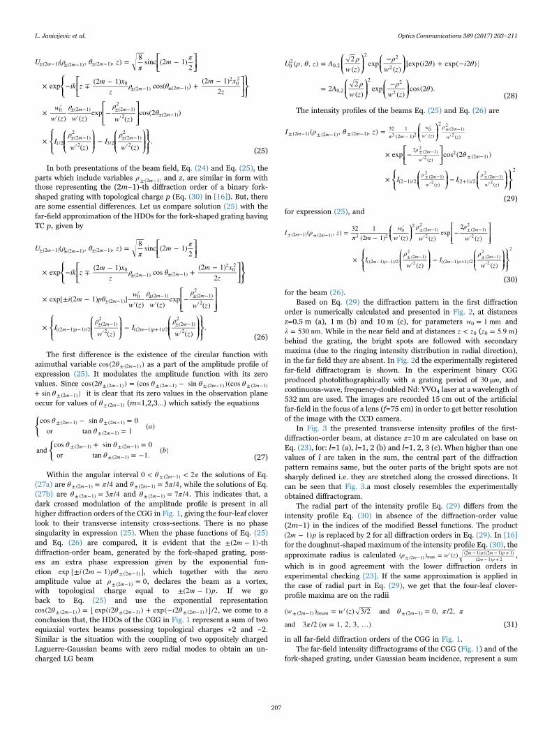
for the beam (26).Based on Eq. (29) the diffraction pattern in the first diffraction

order is numerically calculated and presented in Fig. 2, at distancesz=0.5 m (a), 1 m (b) and 10 m (c), for parameters w = 1 mm0 andλ = 530 nm. While in the near field and at distances z z< 0 (z = 5.9 m0 )behind the grating, the bright spots are followed with secondarymaxima (due to the ringing intensity distribution in radial direction),in the far field they are absent. In Fig. 2d the experimentally registeredfar-field diffractogram is shown. In the experiment binary CGGproduced photolithographically with a grating period of m30 μ , andcontinuous-wave, frequency-doubled Nd: YVO4 laser at a wavelength of532 nm are used. The images are recorded 15 cm out of the artificialfar-field in the focus of a lens (f=75 cm) in order to get better resolutionof the image with the CCD camera.

In Fig. 3 the presented transverse intensity profiles of the first-diffraction-order beam, at distance z=10 m are calculated on base onEq. (23), for: l=1 (a), l=1, 2 (b) and l=1, 2, 3 (c). When higher than onevalues of l are taken in the sum, the central part of the diffractionpattern remains same, but the outer parts of the bright spots are notsharply defined i.e. they are stretched along the crossed directions. Itcan be seen that Fig. 3.a most closely resembles the experimentallyobtained diffractogram.

The radial part of the intensity profile Eq. (29) differs from theintensity profile Eq. (30) in absence of the diffraction-order value(2m−1) in the indices of the modified Bessel functions. The product

m p(2 − 1) is replaced by 2 for all diffraction orders in Eq. (29). In [16]for the doughnut-shaped maximum of the intensity profile Eq. (30), theapproximate radius is calculated ρ w z( ) = ′( )m

m p m pm p± (2 −1) max

(2 − 1) ((2 − 1) + 1)(2 − 1) + 2

,

which is in good agreement with the lower diffraction orders inexperimental checking [23]. If the same approximation is applied inthe case of radial part in Eq. (29), we get that the four-leaf clover-profile maxima are on the radii

w w z θ π π

π m

( ) = ′( ) 3/2 and = 0, /2,

and 3 /2 ( = 1, 2, 3, …)m beam m± (2 −1) ± (2 −1)

(31)

in all far-field diffraction orders of the CGG in Fig. 1.The far-field intensity diffractograms of the CGG (Fig. 1) and of the

fork-shaped grating, under Gaussian beam incidence, represent a sum

L. Janicijevic et al. Optics Communications 389 (2017) 203–211

207

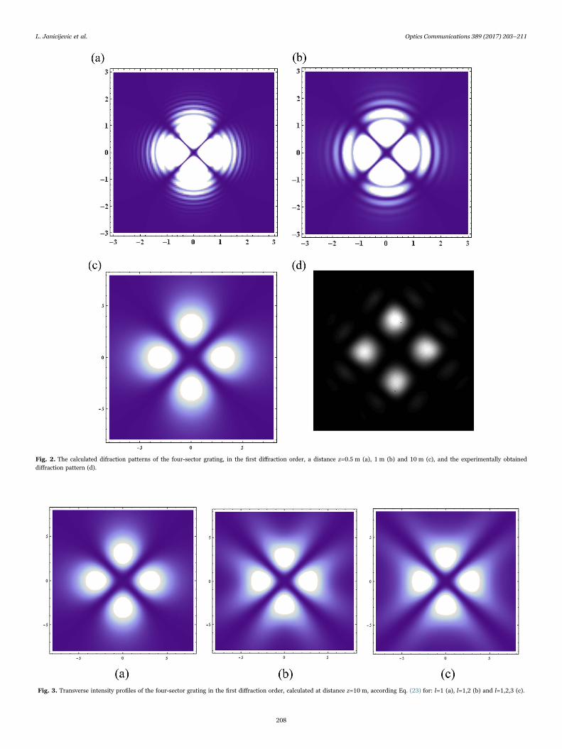
Fig. 2. The calculated difraction patterns of the four-sector grating, in the first diffraction order, a distance z=0.5 m (a), 1 m (b) and 10 m (c), and the experimentally obtaineddiffraction pattern (d).

Fig. 3. Transverse intensity profiles of the four-sector grating in the first diffraction order, calculated at distance z=10 m, according Eq. (23) for: l=1 (a), l=1,2 (b) and l=1,2,3 (c).

L. Janicijevic et al. Optics Communications 389 (2017) 203–211

208

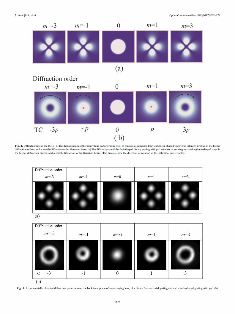
Fig. 4. Diffractograms of the CGGs: a) The diffractogram of the binary four-sector grating (Fig. 1) consists of equisized four-leaf clover-shaped transverse intensity profiles in the higherdiffraction orders, and a zeroth-diffraction-order Gaussian beam. b) The diffractogram of the fork-shaped binary grating with p=1 consists of growing in size doughnut-shaped rings inthe higher diffraction orders, and a zeroth-diffraction-order Gaussian beam. (The arrows show the direction of rotation of the helicoidal wave fronts).

Fig. 5. Experimentally obtained diffraction patterns near the back focal plane of a converging lens, of a binary four-sectorial grating (a), and a fork-shaped grating with p=1 (b).

L. Janicijevic et al. Optics Communications 389 (2017) 203–211

209

over all intensity profiles of the separate diffraction-order beamintensities Eq. (29) or Eq. (30). In agreement with the previouslydiscussed theoretical results, it is possible to draw a schematic pictureof the expected look of the diffractograms (Fig. 4) - the numericalcalculation is done at z=10 m, for parameters w = 1 mm0 andλ = 530 nm. While, in Fig. 5 the experimentally obtained diffractionpatterns of a binary, computer-generated four-sector grating (a) and afork-shaped grating with topological charge p=1 (b), registered near(15 cm behind) the back focal plane of a converging lens with focaldistance f=75 cm are presented.

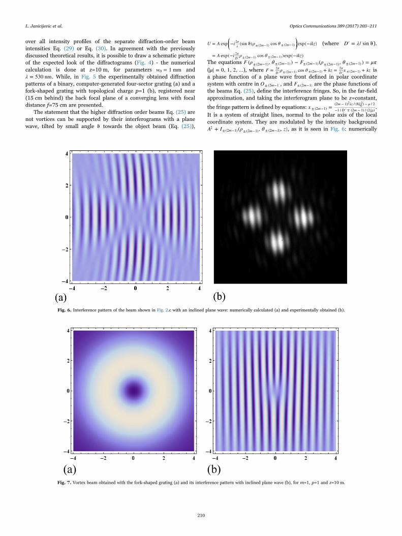
The statement that the higher diffraction order beams Eq. (25) arenot vortices can be supported by their interferograms with a planewave, tilted by small angle ϑ towards the object beam (Eq. (25)),

U A i ρ θ ikz

A i ρ θ ikz

= exp − (sin ϑ) cos exp(− )

= exp(− cos )exp(− )

πλ m m

πD m m

2± (2 −1) ± (2 −1)

2′ ± (2 −1) ± (2 −1)

⎛⎝⎜

⎞⎠⎟ (where D λ′ = / sin ϑ).

The equations F ρ θ F ρ θ μπ( , ) − ( , ) =m m m m m± (2 −1) ± (2 −1) ± (2 −1) ± (2 −1) ± (2 −1)

(μ = 0, 1, 2, ...), where F ρ θ kz x kz= cos + = +πD m m

πD m

2′ ± (2 −1) ± (2 −1)

2′ ± (2 −1) is

a phase function of a plane wave front defined in polar coordinatesystem with centre in O m± (2 −1), and F m± (2 −1) are the phase functions ofthe beams Eq. (25), define the interference fringes. So, in the far-fieldapproximation, and taking the interferogram plane to be z=constant,

the fringe pattern is defined by equations: x =mm λz ξ μ

D m ζ± (2 −1)(2 − 1) / (8 ) − / 2−1 / ′ ∓ (2 − 1) / (2 )

202

0.

It is a system of straight lines, normal to the polar axis of the localcoordinate system. They are modulated by the intensity backgroundA I ρ θ z+ ( , , )m m m

2± (2 −1) ± (2 −1) ± (2 −1) , as it is seen in Fig. 6: numerically

Fig. 6. Interference pattern of the beam shown in Fig. 2.c with an inclined plane wave: numerically calculated (a) and experimentally obtained (b).

Fig. 7. Vortex beam obtained with the fork-shaped grating (a) and its interference pattern with inclined plane wave (b), for m=1, p=1 and z=10 m.

L. Janicijevic et al. Optics Communications 389 (2017) 203–211

210

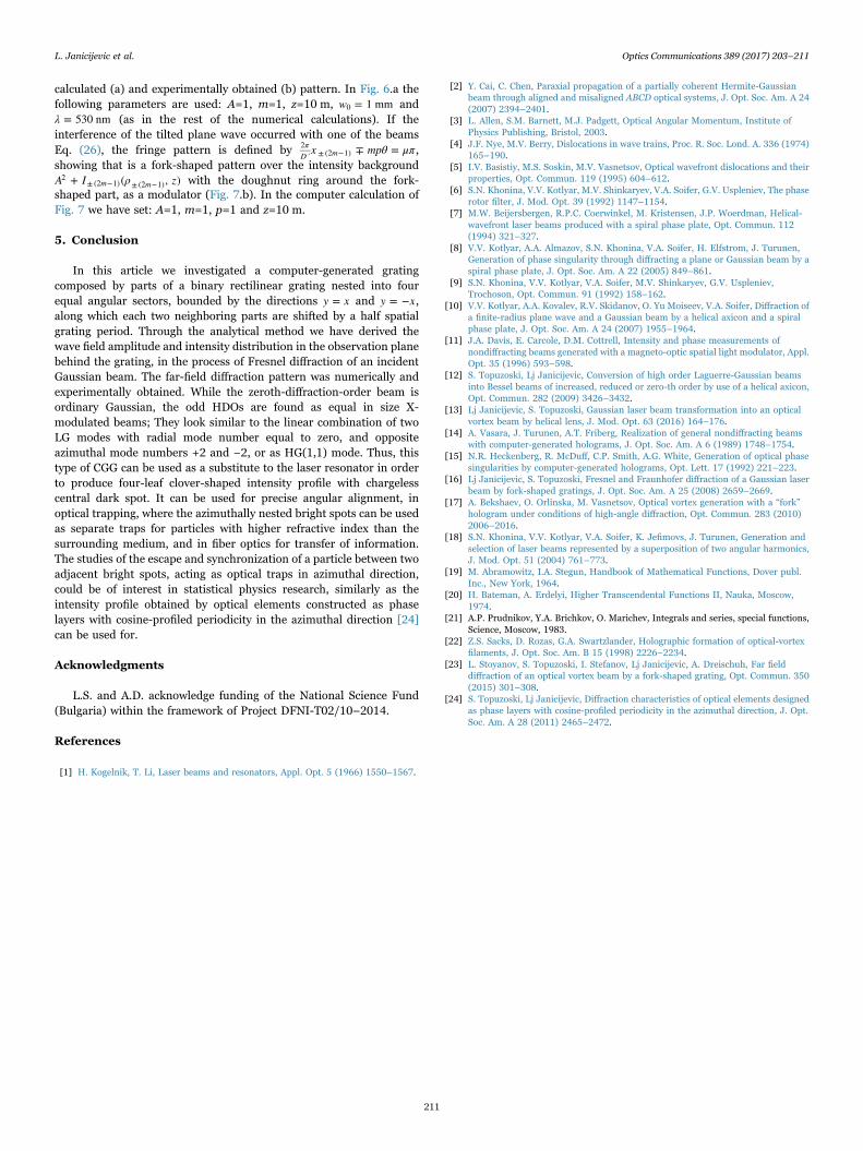
calculated (a) and experimentally obtained (b) pattern. In Fig. 6.a thefollowing parameters are used: A=1, m=1, z=10 m, w = 1 mm0 andλ = 530 nm (as in the rest of the numerical calculations). If theinterference of the tilted plane wave occurred with one of the beamsEq. (26), the fringe pattern is defined by x mpθ μπ∓ =π

D m2

′ ± (2 −1) ,showing that is a fork-shaped pattern over the intensity backgroundA I ρ z+ ( , )m m

2± (2 −1) ± (2 −1) with the doughnut ring around the fork-

shaped part, as a modulator (Fig. 7.b). In the computer calculation ofFig. 7 we have set: A=1, m=1, p=1 and z=10 m.

5. Conclusion

In this article we investigated a computer-generated gratingcomposed by parts of a binary rectilinear grating nested into fourequal angular sectors, bounded by the directions y x= and y x= − ,along which each two neighboring parts are shifted by a half spatialgrating period. Through the analytical method we have derived thewave field amplitude and intensity distribution in the observation planebehind the grating, in the process of Fresnel diffraction of an incidentGaussian beam. The far-field diffraction pattern was numerically andexperimentally obtained. While the zeroth-diffraction-order beam isordinary Gaussian, the odd HDOs are found as equal in size X-modulated beams; They look similar to the linear combination of twoLG modes with radial mode number equal to zero, and oppositeazimuthal mode numbers +2 and −2, or as HG(1,1) mode. Thus, thistype of CGG can be used as a substitute to the laser resonator in orderto produce four-leaf clover-shaped intensity profile with chargelesscentral dark spot. It can be used for precise angular alignment, inoptical trapping, where the azimuthally nested bright spots can be usedas separate traps for particles with higher refractive index than thesurrounding medium, and in fiber optics for transfer of information.The studies of the escape and synchronization of a particle between twoadjacent bright spots, acting as optical traps in azimuthal direction,could be of interest in statistical physics research, similarly as theintensity profile obtained by optical elements constructed as phaselayers with cosine-profiled periodicity in the azimuthal direction [24]can be used for.

Acknowledgments

L.S. and A.D. acknowledge funding of the National Science Fund(Bulgaria) within the framework of Project DFNI-T02/10–2014.

References

[1] H. Kogelnik, T. Li, Laser beams and resonators, Appl. Opt. 5 (1966) 1550–1567.

[2] Y. Cai, C. Chen, Paraxial propagation of a partially coherent Hermite-Gaussianbeam through aligned and misaligned ABCD optical systems, J. Opt. Soc. Am. A 24(2007) 2394–2401.

[3] L. Allen, S.M. Barnett, M.J. Padgett, Optical Angular Momentum, Institute ofPhysics Publishing, Bristol, 2003.

[4] J.F. Nye, M.V. Berry, Dislocations in wave trains, Proc. R. Soc. Lond. A. 336 (1974)165–190.

[5] I.V. Basistiy, M.S. Soskin, M.V. Vasnetsov, Optical wavefront dislocations and theirproperties, Opt. Commun. 119 (1995) 604–612.

[6] S.N. Khonina, V.V. Kotlyar, M.V. Shinkaryev, V.A. Soifer, G.V. Uspleniev, The phaserotor filter, J. Mod. Opt. 39 (1992) 1147–1154.

[7] M.W. Beijersbergen, R.P.C. Coerwinkel, M. Kristensen, J.P. Woerdman, Helical-wavefront laser beams produced with a spiral phase plate, Opt. Commun. 112(1994) 321–327.

[8] V.V. Kotlyar, A.A. Almazov, S.N. Khonina, V.A. Soifer, H. Elfstrom, J. Turunen,Generation of phase singularity through diffracting a plane or Gaussian beam by aspiral phase plate, J. Opt. Soc. Am. A 22 (2005) 849–861.

[9] S.N. Khonina, V.V. Kotlyar, V.A. Soifer, M.V. Shinkaryev, G.V. Uspleniev,Trochoson, Opt. Commun. 91 (1992) 158–162.

[10] V.V. Kotlyar, A.A. Kovalev, R.V. Skidanov, O. Yu Moiseev, V.A. Soifer, Diffraction ofa finite-radius plane wave and a Gaussian beam by a helical axicon and a spiralphase plate, J. Opt. Soc. Am. A 24 (2007) 1955–1964.

[11] J.A. Davis, E. Carcole, D.M. Cottrell, Intensity and phase measurements ofnondiffracting beams generated with a magneto-optic spatial light modulator, Appl.Opt. 35 (1996) 593–598.

[12] S. Topuzoski, Lj Janicijevic, Conversion of high order Laguerre-Gaussian beamsinto Bessel beams of increased, reduced or zero-th order by use of a helical axicon,Opt. Commun. 282 (2009) 3426–3432.

[13] Lj Janicijevic, S. Topuzoski, Gaussian laser beam transformation into an opticalvortex beam by helical lens, J. Mod. Opt. 63 (2016) 164–176.

[14] A. Vasara, J. Turunen, A.T. Friberg, Realization of general nondiffracting beamswith computer-generated holograms, J. Opt. Soc. Am. A 6 (1989) 1748–1754.

[15] N.R. Heckenberg, R. McDuff, C.P. Smith, A.G. White, Generation of optical phasesingularities by computer-generated holograms, Opt. Lett. 17 (1992) 221–223.

[16] Lj Janicijevic, S. Topuzoski, Fresnel and Fraunhofer diffraction of a Gaussian laserbeam by fork-shaped gratings, J. Opt. Soc. Am. A 25 (2008) 2659–2669.

[17] A. Bekshaev, O. Orlinska, M. Vasnetsov, Optical vortex generation with a “fork”hologram under conditions of high-angle diffraction, Opt. Commun. 283 (2010)2006–2016.

[18] S.N. Khonina, V.V. Kotlyar, V.A. Soifer, K. Jefimovs, J. Turunen, Generation andselection of laser beams represented by a superposition of two angular harmonics,J. Mod. Opt. 51 (2004) 761–773.

[19] M. Abramowitz, I.A. Stegun, Handbook of Mathematical Functions, Dover publ.Inc., New York, 1964.

[20] H. Bateman, A. Erdelyi, Higher Transcendental Functions II, Nauka, Moscow,1974.

[21] A.P. Prudnikov, Y.A. Brichkov, O. Marichev, Integrals and series, special functions,Science, Moscow, 1983.

[22] Z.S. Sacks, D. Rozas, G.A. Swartzlander, Holographic formation of optical-vortexfilaments, J. Opt. Soc. Am. B 15 (1998) 2226–2234.

[23] L. Stoyanov, S. Topuzoski, I. Stefanov, Lj Janicijevic, A. Dreischuh, Far fielddiffraction of an optical vortex beam by a fork-shaped grating, Opt. Commun. 350(2015) 301–308.

[24] S. Topuzoski, Lj Janicijevic, Diffraction characteristics of optical elements designedas phase layers with cosine-profiled periodicity in the azimuthal direction, J. Opt.Soc. Am. A 28 (2011) 2465–2472.

L. Janicijevic et al. Optics Communications 389 (2017) 203–211

211