diffusion and strategic interaction on social...

Diffusion and Strategic Interaction on Social Networks

Leeat Yariv Jerusalem Summer School, June 28, 2016

Questions:

p  How do choices to invest in education, learn a language, etc., depend on social network structure and location within a network? How does network structure impact behavior and

welfare? How does relative position in a network impact

behavior and welfare?

How does behavior propagate through network (important for marketing, epidemiology, etc.)?

Questions:

p  How do choices to invest in education, learn a language, etc., depend on social network structure and location within a network?

n  How does network structure impact behavior and welfare?

n  How does relative location in a network impact behavior and welfare?

How does behavior propagate through

network (important for marketing, epidemiology, etc.)?

Questions:

p  How do choices to invest in education, learn a language, etc., depend on social network structure and location within a network?

n  How does network structure impact behavior and welfare?

n  How does relative location in a network impact behavior and welfare?

p  How does behavior propagate through networks (important for marketing, epidemiology, etc.)?

Choices without Networks: Some History

p Morton Grodzins (1957) coined the term tipping point when explaining white flight

p Tipping Point: A time in which a large number of individuals rapidly and dramatically change behavior

Card, Mas, and Rothstein (2008)

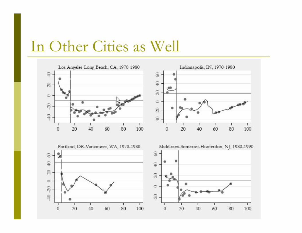
In Other Cities as Well

Schelling (1969, 1971) p  “A general theory of tipping”

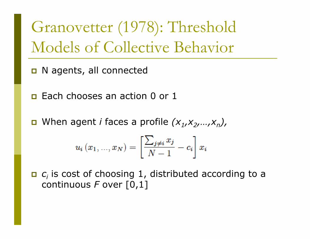
Granovetter (1978): Threshold Models of Collective Behavior p  N agents, all connected

p  Each chooses an action 0 or 1

When agent i faces a profile (x1,x2,…,xn),

ci is cost of choosing 1, distributed according to a continuous F over [0,1] (could be privately or commonly known) (analogous to random thresholds)

Granovetter (1978): Threshold Models of Collective Behavior p  N agents, all connected

p  Each chooses an action 0 or 1

p  When agent i faces a profile (x1,x2,…,xn),

p  ci is cost of choosing 1, distributed according to a continuous F over [0,1]

(could be privately or commonly known) (analogous to random thresholds)

Granovetter (1978) p  Assume at each stage agents best respond to

previous period’s action distribution

uppose at period t a fraction xt choose 1

At period t+1, adopt ßà

≥ ci

For N large,

≈ xt

Granovetter (1978) p  Assume at each stage agents best respond to

previous period’s action distribution

p  Suppose at period t a fraction xt choose 1

p  At period t+1, adopt ßà

≥ ci

p  For N large,

≈ xt

Equilibrium in Granovetter p  Approximated transition formula:

xt+1 ≈ F(xt)

p  A fixed point x* = F(x*) is an equilibrium

The shape of F determines which equilibria are tipping points (more formal soon)

[ Contrast with Bass’ G(t) ]

Equilibrium in Granovetter p  Approximated transition formula:

xt+1 ≈ F(xt)

p  A fixed point x* = F(x*) is an equilibrium

p  The shape of F determines which equilibria are tipping points (more formal soon)

p  [ Contrast with Bass’ F(t) ]

S-shape Adoption in Granovetter (1978) p  Level of change:

The derivative of F(x)-x is F’(x)-1

S-shape à F’(x) > 1 up to some point and F’(x) < 1 afterwards

t

xt

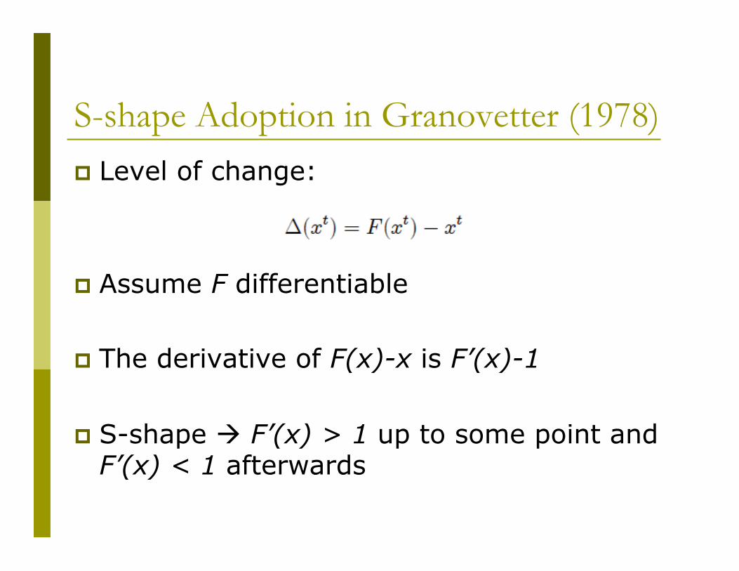
S-shape Adoption in Granovetter (1978) p  Level of change:

p Assume F differentiable

p  The derivative of F(x)-x is F’(x)-1

p S-shape à F’(x) > 1 up to some point and F’(x) < 1 afterwards

Introducing Networks

p So far, no networks

p How does network architecture affect diffusion?

p How does location within a network affect diffusion (recall the adoption of Tetracycline…)?

Example - Experimentation Knowing the Network Structure

p  Suppose you gain 1 if anyone experiments, 0 otherwise, but experimentation is costly (grains, software, etc.)

Example - Experimentation p  Suppose you gain 1 if anyone experiments, 0

otherwise, but experimentation is costly (grains, software, etc.) EXPERIMENTATION – 1

NO EXPERIMENTATION - 0

p  Network structure known – multiple stable states: 1

1

11

10

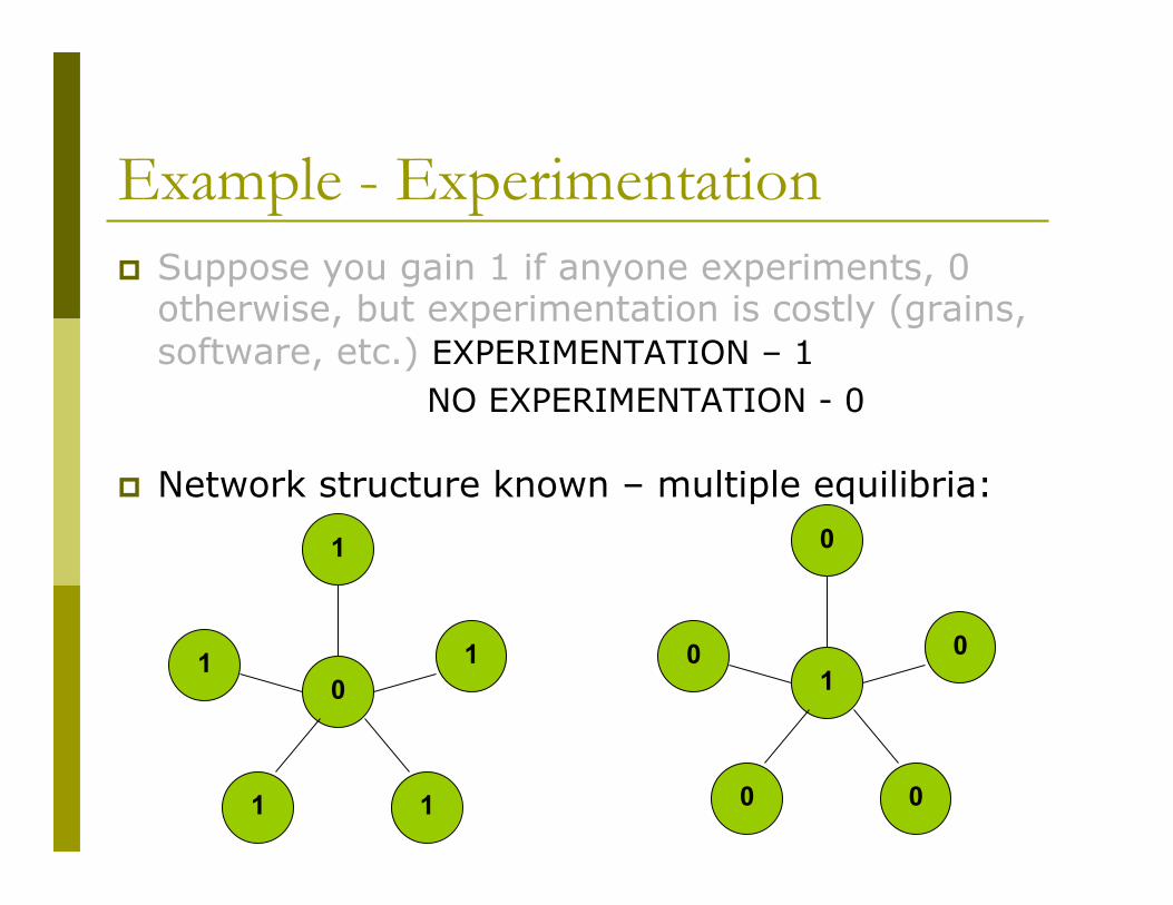
Example - Experimentation p  Suppose you gain 1 if anyone experiments, 0

otherwise, but experimentation is costly (grains, software, etc.) EXPERIMENTATION – 1

NO EXPERIMENTATION - 0

p  Network structure known – multiple equilibria: 1

1

11

10

0

0

00

01

Example – Experimentation (2) Not knowing the structure


p  Probability p of a link between any two agents (Poisson..)


p  Probability p of a link between any two agents

p  Symmetry


p  Probability p of a link between any two agents.

p  Symmetry

p  Probability that a neighbor experiments independent of own degree (number of neighbors) n  → Higher degree less willing to choose 1 n  → Threshold equilibrium: low degrees experiment, high

degrees do not.


p  Probability p of a link between any two agents.

p  Symmetry

p  Probability that a neighbor experiments independent of own degree (number of neighbors) n  → Higher degree less willing to choose 1 n  → Threshold equilibrium: low degrees experiment, high

degrees do not.

p  Strong dependence on p n  p=0→ all choose 1, n  p=1→ all choose 1 with probability 1-c1/(n-1)

General Messages p  Information Matters


p  Location Matters n  Monotonicity with respect to degrees

p  Regarding behavior (complementarities…) p  Regarding expected benefits (externalities…)


p  Location Matters n  Monotonicity with respect to degrees

p  Regarding behavior (complementarities…) p  Regarding expected benefits (externalities…)

p Network Structure Matters n  Adding links affects behavior monotonically

(complementarities…) n  Increasing heterogeneity?

Challenge

p Complexity of networks

p  Tractable way to study behavior outside of simple (regular structures)?

Focus on key characteristics:

p Degree Distribution p How connected is the network?

n  average degree, FOSD shifts

p How are links distributed across agents? n  variance, skewness, etc.

Network Games – Payoff Structure

p  Actions in {0,1}

Action 0: Normalize payoff to 0

Action 1: payoffs depend on number of neighbors choosing 1

Normalize payoff of all neighbors choosing 0 to 0

v(d,x) – ci payoff from choosing 1 if degree is d and a fraction x of neighbors choose 1

Increasing in x

ci distributed according to H, with no atoms



p  Action 0: Normalize payoff to 0

Action 1: payoffs depend on number of neighbors choosing 1

Normalize payoff of all neighbors choosing 0 to 0


Increasing in x





p  Action 1: payoffs depend on number of neighbors choosing 1


Increasing in x





p  Action 1: payoffs depend on number of neighbors choosing 1

p  v(d,x) – ci payoff from choosing 1 if degree is d and a fraction x of neighbors choose 1

p  ci distributed according to H, with no atoms

Examples (payoff: v(d,x)-c)

p  Average Action: v(d,x)=v(d)x= x (classic coordination games, choice of technology)

p  Total Number: v(d,x)=v(d)x=dx (learn a new language, need partners to use new good or

technology, need to hear about it to learn)

p  Critical Mass: v(d,x)=0 for x up to some M/d and v(d,x)=1 above M/d

(uprising, voting, …)

p  Decreasing: v(d,x) declining in d (information aggregation, lower degree correlated with

leaning towards adoption)

Network Games – Information

p  (today) Incomplete information n  know only own degree and assume others’

types are governed by degree distribution n  presume no correlation in degree n  Bayesian equilibrium – as function of degree

Incomplete Information

p  g drawn from some set of networks G such that (assuming large population): n  degrees of neighbors are independent n  Probability of any node having degree d is p(d) n  probability of given neighbor having degree d is

P(d)=dp(d)/E(d)



P(d)=dp(d)/E(d)

2

1

1

p(2)=1/2

p(1)=1/2



P(d)=dp(d)/E(d)

2

1

1

Probability of hitting 2 is twice as high as that of hitting 1 → P(2)=2/3.


p  g drawn from some set of networks G such that: n  degrees of neighbors are independent n  Probability of any node having degree d is p(d) n  probability of given neighbor having degree d is

P(d)=dp(d)/E(d)

p  type of i is ( di(g), ci ); space of types Ti


p  g drawn from some set of networks G such that: n  degrees of neighbors are independent n  Probability of any node having degree d is p(d) n  probability of given neighbor having degree d is

P(d)=dp(d)/E(d)

p  type of i is ( di(g), ci ); space of types Ti p  strategy: σi: Ti→ Δ(X)

Equilibrium as a fixed point:

p Adopt if and only if v(d,x) – ci ≥ 0

p H(v(d,x)) is the percent of degree d types adopting action 1 if x is fraction of random neighbors adopting

Equilibrium corresponds to a fixed point: x = φ(x) = ∑ P(d) H(v(d,x)) = ∑ d p(d) H(v(d,x)) / E[d]


p Adopt if and only if v(d,x) – ci ≥ 0


p  Equilibrium corresponds to a fixed point: x = φ(x) = ∑ P(d) H(v(d,x)) = ∑ d p(d) H(v(d,x)) / E[d]



p  Equilibrium corresponds to a fixed point: x = φ(x) = ∑ P(d) H(v(d,x)) p v continuous in x ! fixed point exists

Monotone Behavior

Observation 1: In a game of incomplete information, every symmetric

equilibrium is monotone p  Non-decreasing in degree if v(d,x) is increasing in d p  Non-increasing in degree if v(d,x) is decreasing in d

Monotone Behavior Intuition p  Symmetric equilibrium – a random neighbor has

probability x of choosing 1, probability 1-x of choosing 0

Monotone Behavior Intuition p  Symmetric equilibrium – a random neighbor has

probability x of choosing 1, probability 1-x of choosing 0

p  Consider agent of degree d+1 n  v(d,x) non-decreasing → payoff from 1 is v(d+1,x)≥v(d,x) n  v(d,x) non-increasing → payoff from 1 is v(d+1,x)≤v(d,x)

Diffusion x = φ(x) = ∑ P(d) H(v(d,x))

p  start with some x0

p  let x1 = φ( x0), xt = φ(xt-1), ...

Interpretations examining equilibrium set with incomplete information

Stable equilibria are converged to from above and below looking at diffusion: complete information best response

dynamics on “large, well-mixed” social network

Diffusion x = φ(x) = ∑ P(d) H(v(d,x))

p  start with some x0

p  let x1 = φ( x0), xt = φ(xt-1), ...

p  Interpretations n  examining equilibrium set with incomplete information

p  Stable equilibria are converged to from above and below n  looking at diffusion: best response dynamics on “large, well-

mixed” social network (mean-field approximation)

xt+1

xt

φ (x)

tipping point unstable equilibrium

stable equilibrium 0

xt+1

xt

φ (x)

0 x0

x1

xt+1

xt

φ (x)

0 x0

x1

x1

x2

xt+1

xt

φ (x)

0 x0

x1

x1

x2

x2 … lim xt

xt+1

xt

φ (x)

tipping point unstable equilibrium

stable equilibrium 0

How can we relate structure (network or payoff) to diffusion?

p Concentrate on “regular” environments – no tangencies

p  Tipping and stable points alternate

p Keep track of how φ shifts with changes

xt+1

xt

φ (x)

φ’(x)

tipping point moves down

stable equilibrium moves up

Adding Links p  Consider a FOSD shift in distribution P(d)

n  More weight on higher degrees n  v(d,x) non-decreasing in d à Higher expectations of

higher actions (Observation 1) n  More likely to take higher action

If v(d,x) is nondecreasing in d, then this leads to a pointwise increase of

φ (x) = ∑ P(d) H(v(d,x))

lower tipping point and higher stable equilibrium




p  If v(d,x) is non-decreasing in d, then this leads to a point-wise increase of

φ (x) = ∑ P(d) H(v(d,x))

lower tipping point and higher stable equilibrium





φ (x) = ∑ P(d) H(v(d,x))

p  Lowers tipping points, raises stable equilibria





φ (x) = ∑ P(d) H(v(d,x))

p  Lowers tipping points, raises stable equilibria

p  Does not translate to FOSD shifts in p(d)

Adding Links – Welfare p Suppose v(d,x) non-decreasing in x

p à FOSD shift in P increases payoffs for all agents corresponding to stable equilibria

p à Higher welfare

In general, monotonicity with respect to x (externalities) is important for welfare

Adding Links – Welfare p Suppose v(d,x) non-decreasing in x

p à FOSD shift in P increases payoffs for all agents corresponding to stable equilibria

p à Higher welfare

p  In general, monotonicity with respect to x (externalities) is important for welfare

Raising Costs

p Raising of costs of adoption of action 1 (FOSD shift of H) lowers φ(x) pointwise

n  raises tipping points, lowers stable equilibria

Increasing Variance of Degrees p  v(d,x) increasing convex in d, H convex

n  e.g., v(d,x)=dx, H uniform[0,C] (with high C)

p  p’ is MPS of p implies φ(x) is pointwise higher under p’

p  Roughly, increasing variance leads to lower tipping points and higher stable equilibria

p  Fixing means, φpower(x) ≥ φPoisson(x) ≥ φregular(x)

Can we relate the payoff structure to equilibrium?

p Assume v(d,x)=v(d)x p Vary v(d)

p  If we can influence v, whom should we target to shift equilibrium?

Proposition: impact of v(d) Consider changing v(d) by rearranging its ordering If p(d)d increasing, then v(d) increasing raises φ(x)

pointwise (raises stable equilibria, lowers unstable) [e.g., p is uniform] If p(d)d decreasing, then v(d) decreasing raises φ(x)

pointwise (lowers stable equilibria, raises unstable) [e.g., p is power]

Proposition: impact of v(d) Consider changing v(d) by rearranging its ordering. If p(d)d increasing, then v(d) increasing raises φ(x)

pointwise (raises stable equilibria, lowers unstable) [e.g., p is uniform] If p(d)d decreasing, then v(d) decreasing raises φ(x)

pointwise [e.g., p is power]

Optimal Targeting

p Goes against idea of “targeting” high degree nodes

p Want the most probable neighbors to have the best incentives to adopt

Adoption Across Degrees

p  If v(d,x) is increasing in d, then higher d adopt in higher percentage for each x n  adoption fraction is H(v(d,x)) which is

increasing

p  Patterns over time – depend on concavity of H

Diffusion Across Degrees

fraction adopting over time, power distribution exponent -2, initial seed x=.03, costs Uniform[1,5], v(d)=d

d=3

d=6

0

0.1

0.2

0.3

0.4

0.5

0.6

0.7

0.8

0.9

1

0 1 2 3 4 5 6 7 8 9 10

Period

d=3d=6d=9d=20

Adoption Rate

d=9 d=20

Tetracycline Adoption (Coleman, Katz, and Menzel, 1966)

Summary:

p  Location matters:

n  v(d,x) increasing in d p more connected adopt “earlier,” at higher rate p have higher expected payoffs

Structure matters: Lower tipping points, raise stable equilibria if:

lower costs (in sense of downward shift FOSD of H) increase in connectedness (shift P in sense of FOSD) MPS of p if v, H (weakly) convex match higher propensity v(d) to more prevalent degrees

p(d)d (want decreasing v for power laws) adoption speeds vary over time depending on curvature of the

cost distribution

Summary:

p  Location matters:

n  v(d,x) increasing in d p more connected adopt “earlier,” at higher rate p have higher expected payoffs

p  Structure matters: n  Lower tipping points, higher stable equilibria if:

p  lower costs (downward shift FOSD of H) p  increase in connectedness (FOSD shift of P) p  MPS of p if v, H (weakly) convex p  match higher propensity v(d) to more prevalent degrees

p(d)d (want decreasing v for power laws) n  adoption speeds vary over time depending on curvature of

the cost distribution

The End

Stability at 0 φ(x)<x in a neighborhood around 0 (joint condition on H, v(d,x), P(d)) If H is continuous, and 0 is stable, then “generically”: next unstable (first tipping point, where volume of adopters grows), next is

stable, etc. “Regular” environment: No tangencies

Speed of adoption over time

If H(0)=0 and H is C2 and increasing p  If H is concave, then φ(x)/x is decreasing

n  Convergence upward slows down, convergence downward speeds up

p  If H is convex, then φ(x)/x is increasing

n  Convergence upward speeds up, convergence downward slows down

diffusion and strategic interaction on social...

Documents