diffusion cloud chamber

Diffusion Cloud Chamber

Alex Welch

1 Abstract

In this experiment a diffusion cloud chamber and Helmholtz coils were used to analyze the energy of beta particles from strontium-90 and cosmic rays. The Helmholtz coils were able to produce a magnetic field with a strength of 0.0141 T with approximately 3 A going into each coil. The experimentally determined mean energy of the beta particles from the Sr-90 was .3081 MeV/c with a standard deviation of .1489, which was less than the accepted energy of .546 MeV/c because the experiment was only able to find one component of the energy of the electron. The cosmic rays that were observed had a range of energies, the highest of which was 2.13 MeV/c. During this experiment the scientist learned about the physics of Peltier cells, rectifiers, Helmholtz coils, cloud chambers, cosmic rays, and radiation.

2 Introduction

The first cloud chamber was invented by C.T.R. Wilson in 1911. This cloud chamber uses pressure changes to supersaturate the vapor in the chamber for track viewing. The diffusion cloud chamber was invented in 1939 by Alexander Langsdorf and takes advantage of temperature differences rather than pressure. [3] The first major discovery made by a cloud chamber was the positron, the antimatter particle of the electron. In 1926 the first positron was observed by Dmitri Skobeltyn, but he did not publish his results because the thought of antimatter had not been conceived yet. He had assumed that the track that he saw was the chance overlapping of two different tracks. He was not the only one to see these “electrons falling back into the source,” but nobody made the leap that what they were seeing was in fact not an equipment malfunction but a positive electron until Anderson in 1932. [4]

This paper was written for Dr. James Dann’s Applied Science Research class in the spring of 2012.

84 Alex Welch

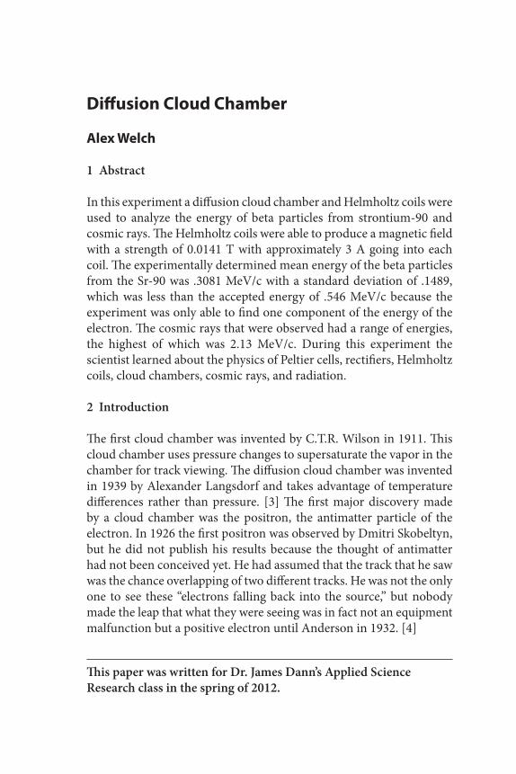
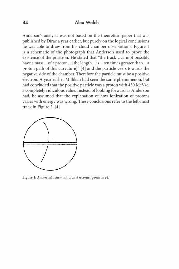
Anderson’s analysis was not based on the theoretical paper that was published by Dirac a year earlier, but purely on the logical conclusions he was able to draw from his cloud chamber observations. Figure 1 is a schematic of the photograph that Anderson used to prove the existence of the positron. He stated that “the track…cannot possibly have a mass…of a proton…[the length…is…ten times greater than…a proton path of this curvature]” [4] and the particle veers towards the negative side of the chamber. Therefore the particle must be a positive electron. A year earlier Millikan had seen the same phenomenon, but had concluded that the positive particle was a proton with 450 MeV/c, a completely ridiculous value. Instead of looking forward as Anderson had, he assumed that the explanation of how ionization of protons varies with energy was wrong. These conclusions refer to the left-most track in Figure 2. [4]

Figure 1: Anderson’s schematic of first recorded positron [4]

THE MENLO ROUNDTABLE 85

Figure 2: Milikan’s schematic positron track in cloud chamber [4]

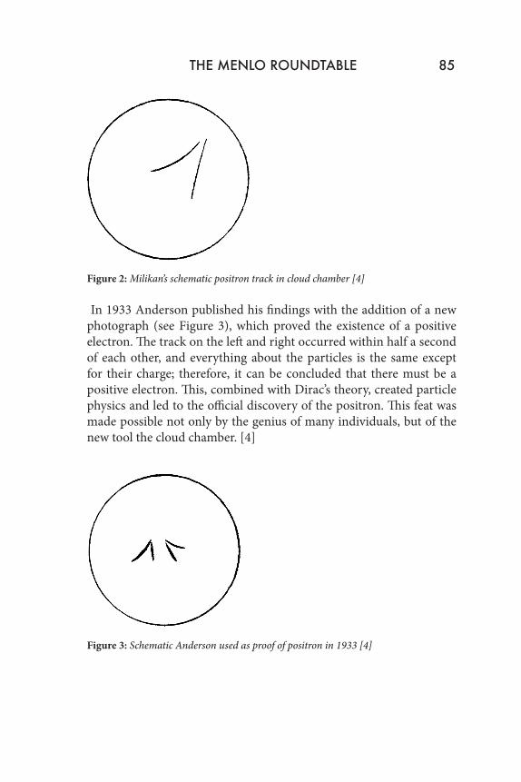
In 1933 Anderson published his findings with the addition of a new photograph (see Figure 3), which proved the existence of a positive electron. The track on the left and right occurred within half a second of each other, and everything about the particles is the same except for their charge; therefore, it can be concluded that there must be a positive electron. This, combined with Dirac’s theory, created particle physics and led to the official discovery of the positron. This feat was made possible not only by the genius of many individuals, but of the new tool the cloud chamber. [4]

Figure 3: Schematic Anderson used as proof of positron in 1933 [4]

86 Alex Welch

Over the next few decades the cloud chamber was used to discover many more particles. In 1937 Neddermeyer and Anderson discovered the muon, by observing a particle that had a unit charge, but a mass that was in between that of an electron and a proton. Then in 1947 Cecil Powell discovered the pion, the particle that transmits the strong force. This discovery was predicted by Yuakawa in 1935, when he observed that protons are held together by a force stronger than the electrostatic force in the nucleus. At this point the world of particles was in symmetry with three leptons and three hadrons, but then two months later Rochester and Butler discovered the strange mason (kaon). They found the particle by observing a cosmic ray that had a mass in between that of pions and protons, but had a longer lifetime than a pion and was only produced in pairs. Scientists then realized just what a multitude of particles must exist and how inadequate the cloud chamber was for finding all of them. This motivated the invention in the 1950s of the particle accelerators in which high energy collisions could be created and many more particles observed. [5]

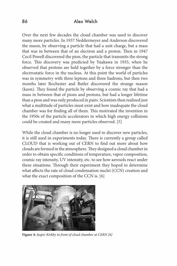
While the cloud chamber is no longer used to discover new particles, it is still used in experiments today. There is currently a group called CLOUD that is working out of CERN to find out more about how clouds are formed in the atmosphere. They designed a cloud chamber in order to obtain specific conditions of temperature, vapor composition, cosmic ray intensity, UV intensity, etc. to see how aerosols react under these situations. Through their experiment they hoped to determine what affects the rate of cloud condensation nuclei (CCN) creation and what the exact composition of the CCN is. [6]

Figure 4: Jasper Kirkby in front of cloud chamber at CERN [6]


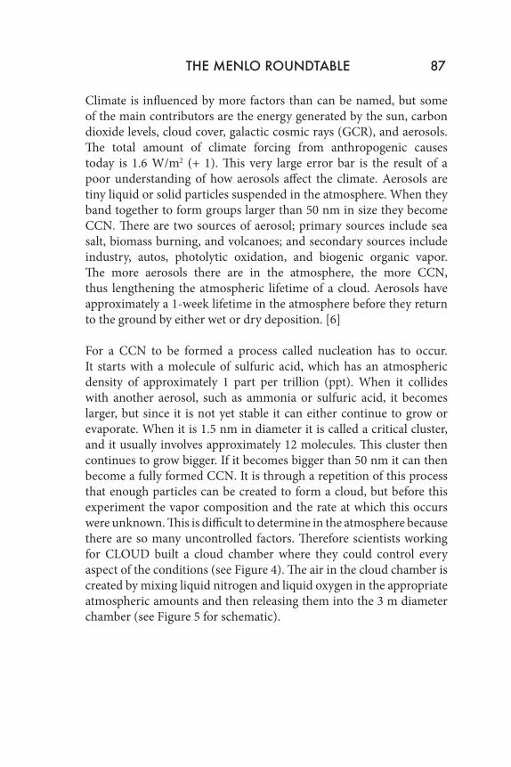
Climate is influenced by more factors than can be named, but some of the main contributors are the energy generated by the sun, carbon dioxide levels, cloud cover, galactic cosmic rays (GCR), and aerosols. The total amount of climate forcing from anthropogenic causes today is 1.6 W/m2 (+ 1). This very large error bar is the result of a poor understanding of how aerosols affect the climate. Aerosols are tiny liquid or solid particles suspended in the atmosphere. When they band together to form groups larger than 50 nm in size they become CCN. There are two sources of aerosol; primary sources include sea salt, biomass burning, and volcanoes; and secondary sources include industry, autos, photolytic oxidation, and biogenic organic vapor. The more aerosols there are in the atmosphere, the more CCN, thus lengthening the atmospheric lifetime of a cloud. Aerosols have approximately a 1-week lifetime in the atmosphere before they return to the ground by either wet or dry deposition. [6]

For a CCN to be formed a process called nucleation has to occur. It starts with a molecule of sulfuric acid, which has an atmospheric density of approximately 1 part per trillion (ppt). When it collides with another aerosol, such as ammonia or sulfuric acid, it becomes larger, but since it is not yet stable it can either continue to grow or evaporate. When it is 1.5 nm in diameter it is called a critical cluster, and it usually involves approximately 12 molecules. This cluster then continues to grow bigger. If it becomes bigger than 50 nm it can then become a fully formed CCN. It is through a repetition of this process that enough particles can be created to form a cloud, but before this experiment the vapor composition and the rate at which this occurs were unknown. This is difficult to determine in the atmosphere because there are so many uncontrolled factors. Therefore scientists working for CLOUD built a cloud chamber where they could control every aspect of the conditions (see Figure 4). The air in the cloud chamber is created by mixing liquid nitrogen and liquid oxygen in the appropriate atmospheric amounts and then releasing them into the 3 m diameter chamber (see Figure 5 for schematic).

88 Alex Welch

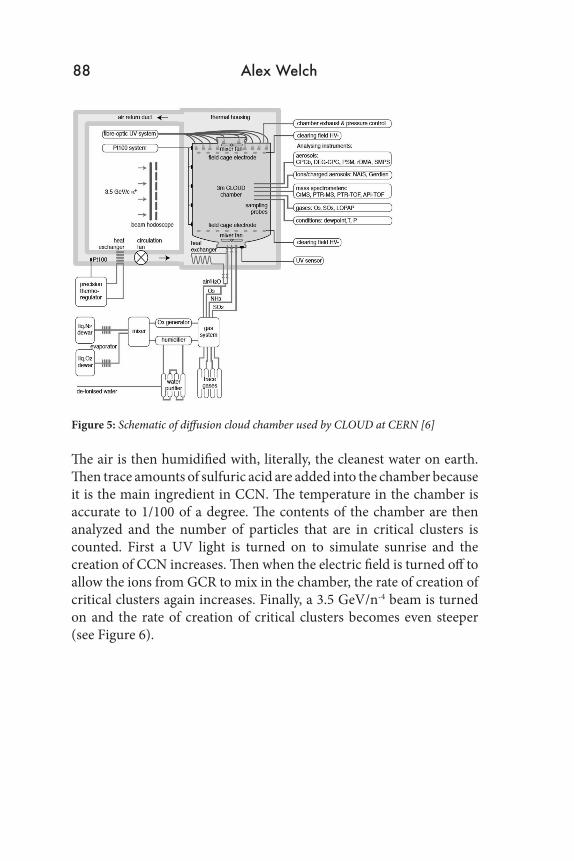
Figure 5: Schematic of diffusion cloud chamber used by CLOUD at CERN [6] The air is then humidified with, literally, the cleanest water on earth. Then trace amounts of sulfuric acid are added into the chamber because it is the main ingredient in CCN. The temperature in the chamber is accurate to 1/100 of a degree. The contents of the chamber are then analyzed and the number of particles that are in critical clusters is counted. First a UV light is turned on to simulate sunrise and the creation of CCN increases. Then when the electric field is turned off to allow the ions from GCR to mix in the chamber, the rate of creation of critical clusters again increases. Finally, a 3.5 GeV/n-4 beam is turned on and the rate of creation of critical clusters becomes even steeper (see Figure 6).


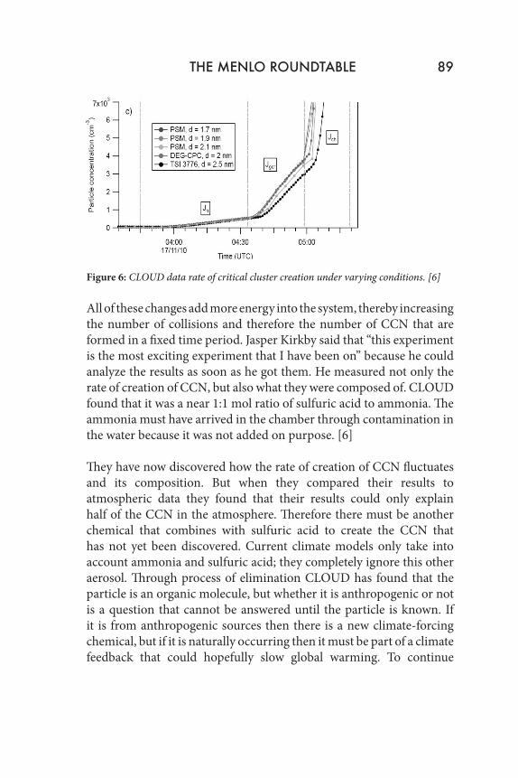
Figure 6: CLOUD data rate of critical cluster creation under varying conditions. [6]

All of these changes add more energy into the system, thereby increasing the number of collisions and therefore the number of CCN that are formed in a fixed time period. Jasper Kirkby said that “this experiment is the most exciting experiment that I have been on” because he could analyze the results as soon as he got them. He measured not only the rate of creation of CCN, but also what they were composed of. CLOUD found that it was a near 1:1 mol ratio of sulfuric acid to ammonia. The ammonia must have arrived in the chamber through contamination in the water because it was not added on purpose. [6]

They have now discovered how the rate of creation of CCN fluctuates and its composition. But when they compared their results to atmospheric data they found that their results could only explain half of the CCN in the atmosphere. Therefore there must be another chemical that combines with sulfuric acid to create the CCN that has not yet been discovered. Current climate models only take into account ammonia and sulfuric acid; they completely ignore this other aerosol. Through process of elimination CLOUD has found that the particle is an organic molecule, but whether it is anthropogenic or not is a question that cannot be answered until the particle is known. If it is from anthropogenic sources then there is a new climate-forcing chemical, but if it is naturally occurring then it must be part of a climate feedback that could hopefully slow global warming. To continue

90 Alex Welch

their research CLOUD is modifying their diffusion cloud chamber into a Wilson chamber so that the actual formation and behavior of clouds can be observed. In conclusion, aerosol nucleation in the lower atmosphere is controlled by unidentified organic vapors together with sulfuric acid and water; and cosmic rays substantially increase the aerosol formation rates under all conditions investigated so far by up to ten times. [6]

The research that these scientists are doing is very important in allowing us to understand how climate change is happening. If we do not understand all of the major causes then there is no hope of being able to stop global warming. Cloud chambers allow these scientists to do their research because of their unique ability to observe particles.

3 Theory

A diffusion cloud chamber allows an observer to ‘see’ radiation, because in the wake of the particle a trail of condensation is formed. This is achieved because of the low temperature in the chamber, the supersaturated alcohol in the air, and the charge of the radioactive particles. [7] In this cloud chamber the cold temperatures will be achieved with a dual stage Peltier cell. [1]

Before the Peltier effect can be discussed, both semiconductors and the Seebeck effect need to be understood. In 1821, only a year after electromagnetism was discovered by Oersted, Seebeck observed that when a magnetic needle is held near a heated dual-metal circuit, it is deflected. Seebeck thought that his discovery meant that magnetization could be caused by a difference in temperature, rather than the fact that a difference in temperature can create a voltage. His discovery was then ignored, but in 1834 Jean Charles Athanase Peltier saw that when current is run through a junction of two different materials a temperature difference is created. Peltier failed to understand the ramifications of his discovery as well, seeing it only as proof that Ohm’s law did not always apply at low currents. Peltier’s discovery was finally understood in 1838 by Emil Lenz, who demonstrated it in a convention in Austria, when “he placed a drop of water on the junction; when


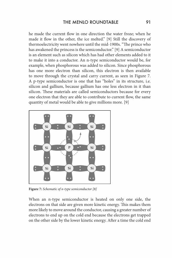
he made the current flow in one direction the water froze; when he made it flow in the other, the ice melted.” [9] Still the discovery of thermoelectricity went nowhere until the mid-1900s. “The prince who has awakened the princess is the semiconductor.” [9] A semiconductor is an element such as silicon which has had other elements added to it to make it into a conductor. An n-type semiconductor would be, for example, when phosphorous was added to silicon. Since phosphorous has one more electron than silicon, this electron is then available to move through the crystal and carry current, as seen in Figure 7. A p-type semiconductor is one that has “holes” in its structure, i.e. silicon and gallium, because gallium has one less electron in it than silicon. These materials are called semiconductors because for every one electron that they are able to contribute to current flow, the same quantity of metal would be able to give millions more. [9]

Figure 7: Schematic of n-type semiconductor [8] When an n-type semiconductor is heated on only one side, the electrons on that side are given more kinetic energy. This makes them more likely to move around the conductor, causing a greater number of electrons to end up on the cold end because the electrons get trapped on the other side by the lower kinetic energy. After a time the cold end

92 Alex Welch

becomes negatively charged relative to the hot end. Therefore, since like charges repel, the electrons begin to move back to the hot end of the conductor. This process goes on until an equilibrium point is reached, where the cold end is more negatively charged than the hot end. This same effect will happen in a p-type semiconductor, but instead of the electrons moving the ‘holes’ will move, giving the cold end a positive charge. When the hot end of the p-type and n-type semiconductors are connected and the cold end of the p-type and n-type semiconductor are connected to form a circuit, current will flow because of the stored charge created by the temperature difference. While the Seebeck effect was first shown on regular metals, the effect is greater by a factor of one hundred in semiconductors because of the relatively few number of electrons they have as compared to a normal metal. While the effect is more pronounced in semiconductors, it still only produces a very small voltage, tenths of a volt for a few hundred degree Centigrade temperature difference. Different semiconductors also create different amounts of voltage per temperature difference because of their different structures. [9]

The mathematical symbol that describes how much a material is affected by the Peltier effect is Π. For a semiconductor at a constant temperature with an electric field, the electric current density jq is equal to

n(-e)(-un)E

where un is the electron mobility of the material. The average energy transported per electron is

(Ec –u) +3/2*kBT

where Ec is the energy at the conduction band edge. The two metals will have the same Fermi level because different conductors in contact have the same Fermi level. The energy flux that accompanies the charge flux is

ju = n(Ec –u +3/2*kBT)(-ue)E


The Peltier coefficient Π is defined by

ju = Π jq

with the units energy carried per unit charge. For electrons

Πe = -(Ec –u +3/2*kBT)/e

and the quantity is negative because the energy flux is in the opposite direction of the charge flux. For holes the Peltier coefficient is

(Ev –u +3/2*kBT)/e

and Ev is energy at the valence band. The Peltier coefficient Π can also be defined as

Π = QT

where Q is the absolute thermoelectric power from the open circuit electric field created by a temperature difference. More simply, the Peltier effect describes how fast electrons move from one place to another. And since different materials have different Π the drift velocity of the electrons is different, which causes a temperature difference. [10] Therefore whenever a voltage is supplied and the electrons begin to move, a temperature difference is created because of how fast the electrons in the different materials move. [3]

More simply, the Peltier effect is just the opposite of what happens when two metals of different temperatures are put together and a voltage is produced, or the Seebeck effect. For example, imagine placing a copper wire and an iron wire next to each other. Since these are different metals the energy that it takes to remove an electron from the outer shell is different. Therefore when the two pieces of metal are placed in contact with each other the electrons will start to move in one direction depending on which metal loses its electrons less easily. This creates a potential difference at the junction. This voltage varies with the temperature of the two metals. The more kinetic energy

94 Alex Welch

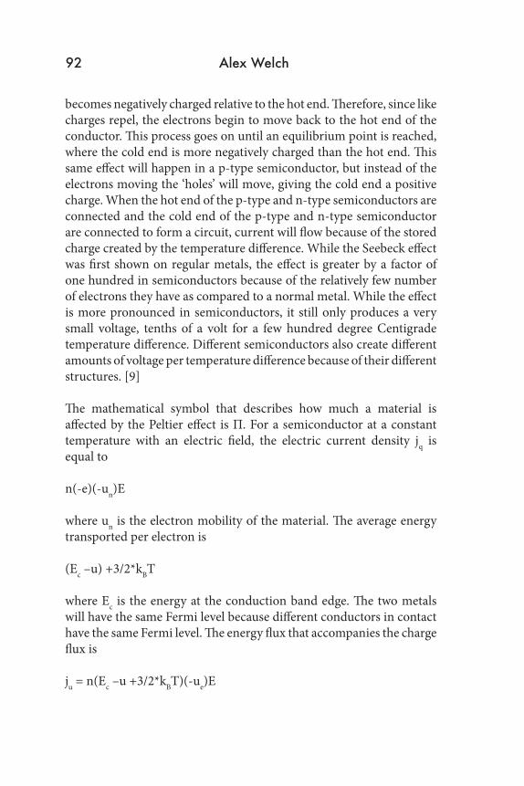
that one side has, the more quickly it can lose its electrons, and the change in how easily a metal loses its electrons with respect to heat is different for different metals. It is therefore clear that by carefully choosing metals and heating or cooling them to specific temperatures a maximum voltage can be produced. The Peltier effect does the same thing, but instead of heating the metals it provides the voltage. Then, by the explanation seen in the previous paragraph or better understood as a “bit of magic”(Keith Jobe), a temperature difference is created. By reversing the linear process the initial input becomes the output. In the Peltier cell used in this project there will be two stacks of semiconductors of different materials, the light grey representing n-type and the dark grey representing p-type, as seen in Figure 8. The bottom layer must be warmer than the above layer. This layer will force the lower part of the top layer to be colder than it would normally be. And since this layer is forcing the topmost layer to be colder than itself, it therefore follows that this top layer is now even colder than it would normally be. That is how the dual-stage Peltier cell achieves such unusually low temperatures. [11] A diffusion cloud chamber needs these super-cold temperatures because otherwise the alcohol will not become saturated enough to form condensation around ions created by passing radiation. [12]

Figure 8: Schematic of a dual-stage Peltier cell


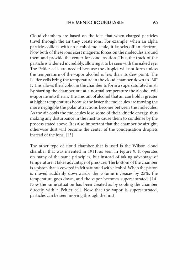
Cloud chambers are based on the idea that when charged particles travel through the air they create ions. For example, when an alpha particle collides with an alcohol molecule, it knocks off an electron. Now both of these ions exert magnetic forces on the molecules around them and provide the center for condensation. Thus the track of the particle is widened incredibly, allowing it to be seen with the naked eye. The Peltier cells are needed because the droplet will not form unless the temperature of the vapor alcohol is less than its dew point. The Peltier cells bring the temperature in the cloud chamber down to -30° F. This allows the alcohol in the chamber to form a supersaturated mist. By starting the chamber out at a normal temperature the alcohol will evaporate into the air. The amount of alcohol that air can hold is greater at higher temperatures because the faster the molecules are moving the more negligible the polar attractions become between the molecules. As the air cools the molecules lose some of their kinetic energy, thus making any disturbance in the mist to cause them to condense by the process stated above. It is also important that the chamber be airtight, otherwise dust will become the center of the condensation droplets instead of the ions. [13]

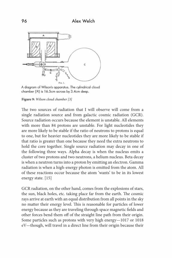
The other type of cloud chamber that is used is the Wilson cloud chamber that was invented in 1911, as seen in Figure 9. It operates on many of the same principles, but instead of taking advantage of temperature it takes advantage of pressure. The bottom of the chamber is a piston that is covered in felt saturated with alcohol. When the piston is moved suddenly downwards, the volume increases by 25%, the temperature goes down, and the vapor becomes supersaturated. [14] Now the same situation has been created as by cooling the chamber directly with a Peltier cell. Now that the vapor is supersaturated, particles can be seen moving through the mist.

96 Alex Welch

Figure 9: Wilson cloud chamber [3] The two sources of radiation that I will observe will come from a single radiation source and from galactic cosmic radiation (GCR). Source radiation occurs because the element is unstable. All elements with more than 84 protons are unstable. For light nucleotides they are more likely to be stable if the ratio of neutrons to protons is equal to one, but for heavier nucleotides they are more likely to be stable if that ratio is greater than one because they need the extra neutrons to hold the core together. Single source radiation may decay in one of the following three ways. Alpha decay is when the nucleus emits a cluster of two protons and two neutrons, a helium nucleus. Beta decay is when a neutron turns into a proton by emitting an electron. Gamma radiation is when a high-energy photon is emitted from the atom. All of these reactions occur because the atom ‘wants’ to be in its lowest energy state. [15]

GCR radiation, on the other hand, comes from the explosions of stars, the sun, black holes, etc. taking place far from the earth. The cosmic rays arrive at earth with an equal distribution from all points in the sky no matter their energy level. This is reasonable for particles of lower energy because as they are traveling through space magnetic fields and other forces bend them off of the straight line path from their origin. Some particles such as protons with very high energy—1017 or 1018 eV—though, will travel in a direct line from their origin because their


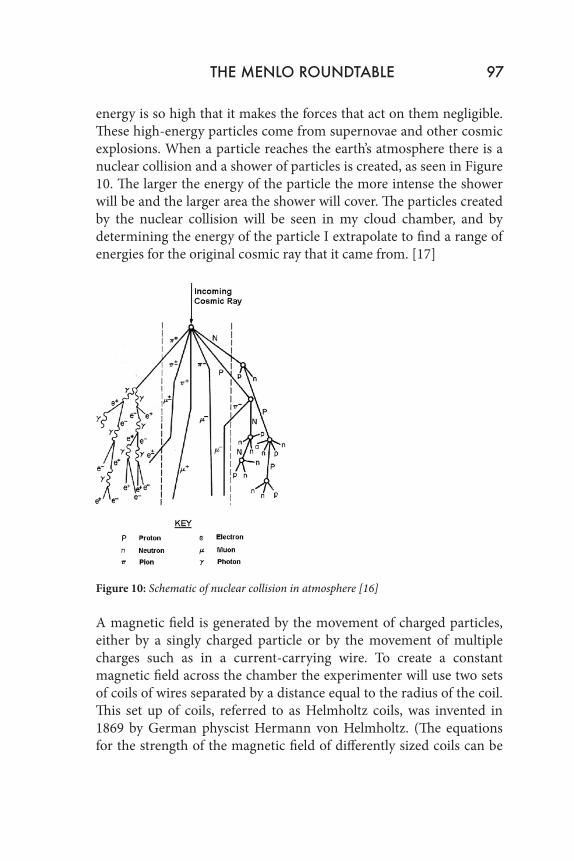
energy is so high that it makes the forces that act on them negligible. These high-energy particles come from supernovae and other cosmic explosions. When a particle reaches the earth’s atmosphere there is a nuclear collision and a shower of particles is created, as seen in Figure 10. The larger the energy of the particle the more intense the shower will be and the larger area the shower will cover. The particles created by the nuclear collision will be seen in my cloud chamber, and by determining the energy of the particle I extrapolate to find a range of energies for the original cosmic ray that it came from. [17]

Figure 10: Schematic of nuclear collision in atmosphere [16] A magnetic field is generated by the movement of charged particles, either by a singly charged particle or by the movement of multiple charges such as in a current-carrying wire. To create a constant magnetic field across the chamber the experimenter will use two sets of coils of wires separated by a distance equal to the radius of the coil. This set up of coils, referred to as Helmholtz coils, was invented in 1869 by German physcist Hermann von Helmholtz. (The equations for the strength of the magnetic field of differently sized coils can be

98 Alex Welch

found in Appendix A.) Unfortunately, in the process of wrapping the coils the radius slowly expands as the wire wraps over itself, making the magnetic field not completely uniform over the entire area. In this experiment, though, the region where particles could be observed was relatively small compared to the size of the coils, so the magnetic field over the active region was fairly uniform, as confirmed by testing with a magnetic field sensor.

4 Results

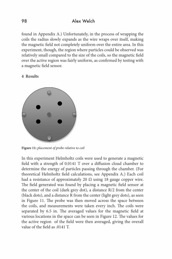
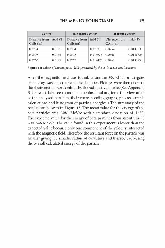
Figure 11: placement of probe relative to coil In this experiment Helmholtz coils were used to generate a magnetic field with a strength of 0.0141 T over a diffusion cloud chamber to determine the energy of particles passing through the chamber. (For theoretical Helmholtz field calculations, see Appendix A.) Each coil had a resistance of approximately 20 Ω using 18 gauge copper wire. The field generated was found by placing a magnetic field sensor at the center of the coil (dark grey dot), a distance R/2 from the center (black dots), and a distance R from the center (light grey dots), as seen in Figure 11. The probe was then moved across the space between the coils, and measurements were taken every inch. The coils were separated by 6.5 in. The averaged values for the magnetic field at various locations in the space can be seen in Figure 12. The values for the active region of the field were then averaged, giving the overall value of the field as .0141 T.

Center R/2 from Center R from CenterDistance from Coils (m)

field (T) Distance from Coils (m)

field (T) Distance from Coils (m)

field (T)

0.0254 0.0175 0.0254 0.02021 0.0254 0.0182330.0508 0.0134 0.0508 0.015675 0.0508 0.01486250.0762 0.0127 0.0762 0.014475 0.0762 0.013325

Figure 12: values of the magnetic field generated by the coils at various locations

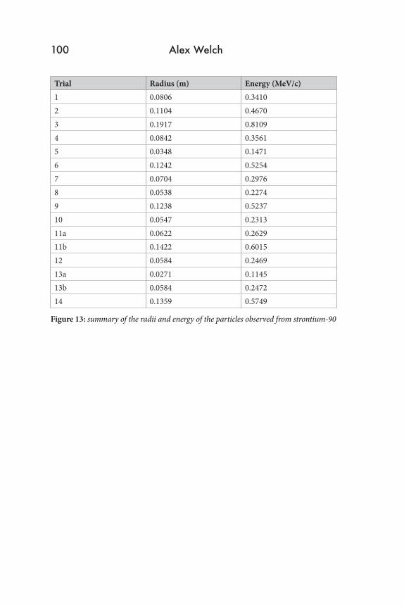
After the magnetic field was found, strontium-90, which undergoes beta decay, was placed next to the chamber. Pictures were then taken of the electrons that were emitted by the radioactive source. (See Appendix B for two trials; see roundtable.menloschool.org for a full view of all of the analyzed particles, their corresponding graphs, photos, sample calculations and histogram of particle energies.) The summary of the results can be seen in Figure 13. The mean value for the energy of the beta particles was .3081 MeV/c with a standard deviation of .1489. The expected value for the energy of beta particles from strontium-90 was .546 MeV/c. The value found in this experiment is lower than the expected value because only one component of the velocity interacted with the magnetic field. Therefore the resultant force on the particle was smaller giving it a smaller radius of curvature and thereby decreasing the overall calculated energy of the particle.


Trial Radius (m) Energy (MeV/c)1 0.0806 0.34102 0.1104 0.46703 0.1917 0.81094 0.0842 0.35615 0.0348 0.14716 0.1242 0.52547 0.0704 0.29768 0.0538 0.22749 0.1238 0.523710 0.0547 0.231311a 0.0622 0.262911b 0.1422 0.601512 0.0584 0.246913a 0.0271 0.114513b 0.0584 0.247214 0.1359 0.5749

Figure 13: summary of the radii and energy of the particles observed from strontium-90

100 Alex Welch

Trial Radius (m) Energy (MeV/c)1a 0.1353 0.57231b 0.1062 0.44922 0.0763 0.32263 0.1346 0.56944 0.0593 0.25085 0.0582 0.24626 0.1635 0.69167 0.0354 0.14968 0.0458 0.19359 0.5058 2.139510 0.0524 0.221611 0.0524 0.221612a 0.0643 0.271812b 0.0611 0.2582

Figure 14: summary of the radii and energy of the observed cosmic rays After completing the observation of the radioactive source, the radiation was removed from the room and the same experiment was repeated, but this time in search of cosmic rays. A number of cosmic rays were observed, and a summary of the results can be seen in Figure 14. The highest energy particle had a radius of .5058 m and an energy of 2.140 MeV/c, far exceeding the energy of any of the particles recorded that had originated from the radioactive source in the first experiment. It is possible that this particle was an uncharged particle, such as a neutrino, and the large radius was a result of errors in the procedure rather than actual curvature. The particle could also have been an alpha particle or a muon because these particles’ relatively larger masses would cause them to curve less under a magnetic field. It is impossible, though, to determine the charge of any of the particles because which side of the chamber the particle came in from is unknown.


This experiment successfully determined the energy of a wide range of particles and found an energy distribution for the energy of beta particles emitted from strontium-90.

5 History

When I first started this experiment my plan was to build my own diffusion cloud chamber following the directions from the Instructables website that described how to build a cloud chamber with a Peltier cell. [1] I tried for a month to make the chamber work, but was unable to succeed after numerous modifications. Then I proceeded to work on creating a magnetic field to place around an already existing diffusion cloud chamber. “The Amateur Scientist” [13] recommended that I try to create a magnetic field with a strength of .1 T; this is what prompted me to do 1300 wraps on each coil and begin working on creating a way to convert the AC power from the wall into DC, so that coils would have enough current to create such a large magnetic field.

I learned how to build a full bridge rectifier and how to connect capacitors in parallel to create DC current. [18] I found, though, that by just using a 60 V power supply for each coil I was able to generate .0141 T field, which was large enough to turn the particles. I then started to analyze the beta particles from strontium-90 and cosmic rays. If someone were to continue this experiment they should work to create a more powerful DC current supply, build their own cloud chamber, analyze more sources of radiation, and continue looking for rare cosmic rays.

102 Alex Welch


6 Citations

[1] Olson, Rich. “Make a Cloud Chamber Using Peltier Cell.” Instructables. N.p., 2011. Web. 18 Jan. 2012. <http://www.instructables.com/id/Make-a-Cloud-Chamber-using-Peltier-Coolers/>.

[2] Olson, Rich. “The Nothings Lab Electric Cloud Chamber.” Nothing Labs. N.p., n.d. Web. 4 Feb. 2012. <http://www.nothinglabs.com/electroniccloudchamber/>.

[3] Wikipedia Editors. “Cloud Chamber.” Wikipedia. N.p., 9 Jan. 2012. Web. 4 Feb. 2012. <http://en.wikipedia.org/wiki/Cloud_chamber>.

[4] Hanson, Norwood Russell. “Discovering the Positron.” The British Journal for the Philosophy of Science 12.47 (1961): 194-214. JSTOR. Web. 4 Feb. 2012. <http://www.jstor.org/pss/685207>.

[5] Skwarnicki, Tomasz. “Particle Discoveries.” Physics. N.p., n.d. Web. 5 Feb. 2012. <www.phy.syr.edu/HEPOutreach/PPFest/Tomasz_PartII.ppt>.

[6] Kirkby, Jasper. “Cosmic Rays, Climate and the CERN CLOUD Experiment.” SLAC Colloquium Series. SLAC, Stanford University. 23 Jan. 2012. Lecture.

[7] How Stuff Works, Inc. “Cloud Chamber.” How Stuff Works. N.p., 1998. Web. 18 Jan. 2012. <http://science.howstuffworks.com/dictionary/physics-terms/cloud-chamber-info.htm>.

[8] Voldman, Joel, and Carol Livermore. “Doped Semiconductor.” Flickr. N.p., 2006. Web. 5 Feb. 2012. <http://www.flickr.com/photos/mitopencourseware/3363321260/>.

[9] Joffe, Abram F. “The Revival of Thermoelectricity.” Scientific American 199.5 (1958): 31-37. Print.

[10] Kittel, Charles. Introduction to Solid State Physics. Chichester: John Wiley and Sons, Inc., 1986. Print.

[11] Jobe, Keith. Personal interview. 23 Jan. 2012.

[12] WiseGeek. “What is a Cloud Chamber.” WiseGeek. N.p., 2003. Web. 18 Jan. 2012. <http://www.wisegeek.com/what-is-a-cloud-chamber.htm>.

[13] Stong, C. L. “How to Fit a Diffusion Cloud-Chamber with a Magnet and Other Accessories.” The Amateur Scientist (June 1959): n. pag. Print.

[14] Ingalls, Albert G. “About Home-Made Cloud Chambers and the Fine Telescope of a Portugese Navy Officer.” The Amateur Scientist (Sept. 1952): n. pag. Print.

[15] Zumdahl, Steve. Chemistry. Boston: Houghton Mifflin, 2006. Print.

[16] Bieber, John W. “Cosmic Rays and Earth.” University of Delaware Bartol Research Institute Neutron Monitor Program. N.p., 16 Dec. 2006. Web. 5 Feb. 2012. <http://neutronm.bartol.udel.edu/catch/cr2.html>.

[17] Rossi, Bruno. “High-Energy Cosmic Rays.” Scientific American (1959): 135-146. Print.

[18] Horowitz, Paul. The Art of Electronics. New York: Cambridge University Press, 1989. Print.

[19] “American Wire Gauge .” Wikipedia. N.p., 1 May 2012. Web. 3 May 2012. <http://en.wikipedia.org/wiki/American_wire_gauge>.

104 Alex Welch


7 Acknowledgements

I would like to thank Dr. Dann for inspiring the project and helping me at every turn; Keith Jobe for taking the time to explain the Peltier effect to me and send several helpful articles; Dave Welch for teaching me the value of organization in my experiment; and Vince Dominic for helping me analyze the curvature of my electrons and cosmic rays.

8 Appendices

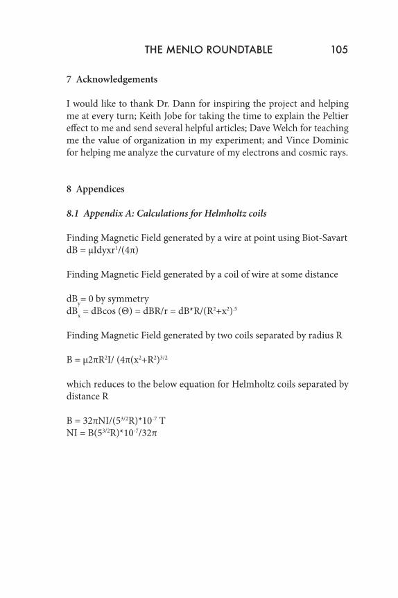
8.1 Appendix A: Calculations for Helmholtz coils

Finding Magnetic Field generated by a wire at point using Biot-SavartdB = μIdyxr1/(4π)

Finding Magnetic Field generated by a coil of wire at some distance

dBy= 0 by symmetrydBx = dBcos (Θ) = dBR/r = dB*R/(R2+x2).5

Finding Magnetic Field generated by two coils separated by radius R

B = μ2πR2I/ (4π(x2+R2)3/2

which reduces to the below equation for Helmholtz coils separated by distance R

B = 32πNI/(53/2R)*10-7 TNI = B(53/2R)*10-7/32π

NI = (.1 T)(53/2.0762m)*107/32πNI = 8474.4 A

Assuming that 5 amps are given to the coils, thenN = 1695

Number of feet of wire requiredNumber of feet = N*2πR = 1695*2π(.0762 m) = 812 m/coil or 2,662.5 ft/coilTotal Wire = 1623 m or 5325 ft

Resistance of CoilResistance of 18 gauge copper wire = 20.95 mΩ/mTotal Resistance = 20.95 mΩ/m * 812 m =17.01 Ω/coil

Mass of Copper per CoilMass = (7.34 g/m)*(1623 m) = 11.91 kg of Cu per Coil

Heat GeneratedP=I2R = (5A)2(17.01 Ω) = 429.0 J/sQ = mC(ΔT)ΔT = (429 J)/(11,914.7 g *.386 J/gK) = .0933 C/s

Current(A)

Number of Coils

Wire per Coil (ft)

Total Wire Needed (ft)

Resistance per coil (Ω)

Power (J/s)

Mass of Wire per Coil (g)

Change in Temperature per Coil (K/s)

1 8474 13430 26860 85.78 85.8 60092 0.004

2 4237 6715 13430 42.89 171.6 30046 0.015

3 2825 4476.7 8953.3 28.59 257.3 20031 0.033

4 2119 3357.5 6715 21.45 343.2 15023 0.059

5 1695 2686 5372 17.16 429.0 12018 0.092

6 1412 2238.3 4476.7 14.3 514.8 10015 0.133

7 1211 1918.6 3837.1 12.25 600.3 8584 0.181

Figure 15: Amount of current, coils, and wire needed to create a .1 T field with Helmholtz coils with 18 gauge copper wire [19]

106 Alex Welch


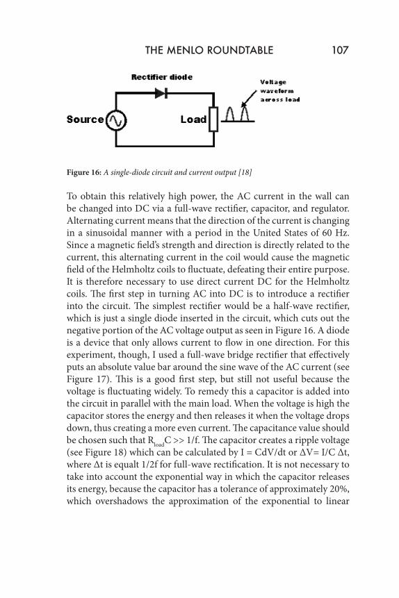
Figure 16: A single-diode circuit and current output [18]

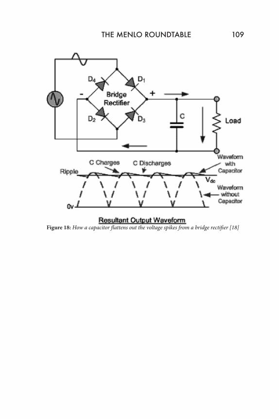
To obtain this relatively high power, the AC current in the wall can be changed into DC via a full-wave rectifier, capacitor, and regulator. Alternating current means that the direction of the current is changing in a sinusoidal manner with a period in the United States of 60 Hz. Since a magnetic field’s strength and direction is directly related to the current, this alternating current in the coil would cause the magnetic field of the Helmholtz coils to fluctuate, defeating their entire purpose. It is therefore necessary to use direct current DC for the Helmholtz coils. The first step in turning AC into DC is to introduce a rectifier into the circuit. The simplest rectifier would be a half-wave rectifier, which is just a single diode inserted in the circuit, which cuts out the negative portion of the AC voltage output as seen in Figure 16. A diode is a device that only allows current to flow in one direction. For this experiment, though, I used a full-wave bridge rectifier that effectively puts an absolute value bar around the sine wave of the AC current (see Figure 17). This is a good first step, but still not useful because the voltage is fluctuating widely. To remedy this a capacitor is added into the circuit in parallel with the main load. When the voltage is high the capacitor stores the energy and then releases it when the voltage drops down, thus creating a more even current. The capacitance value should be chosen such that RloadC >> 1/f. The capacitor creates a ripple voltage (see Figure 18) which can be calculated by I = CdV/dt or ΔV= I/C Δt, where Δt is equalt 1/2f for full-wave rectification. It is not necessary to take into account the exponential way in which the capacitor releases its energy, because the capacitor has a tolerance of approximately 20%, which overshadows the approximation of the exponential to linear

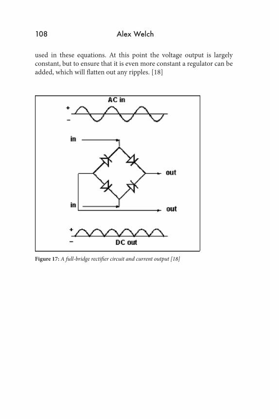
used in these equations. At this point the voltage output is largely constant, but to ensure that it is even more constant a regulator can be added, which will flatten out any ripples. [18]

Figure 17: A full-bridge rectifier circuit and current output [18]

108 Alex Welch


Figure 18: How a capacitor flattens out the voltage spikes from a bridge rectifier [18]

8.2 Appendix B: Trials

For full appendix with all trials, go to roundtable.menloschool.org.

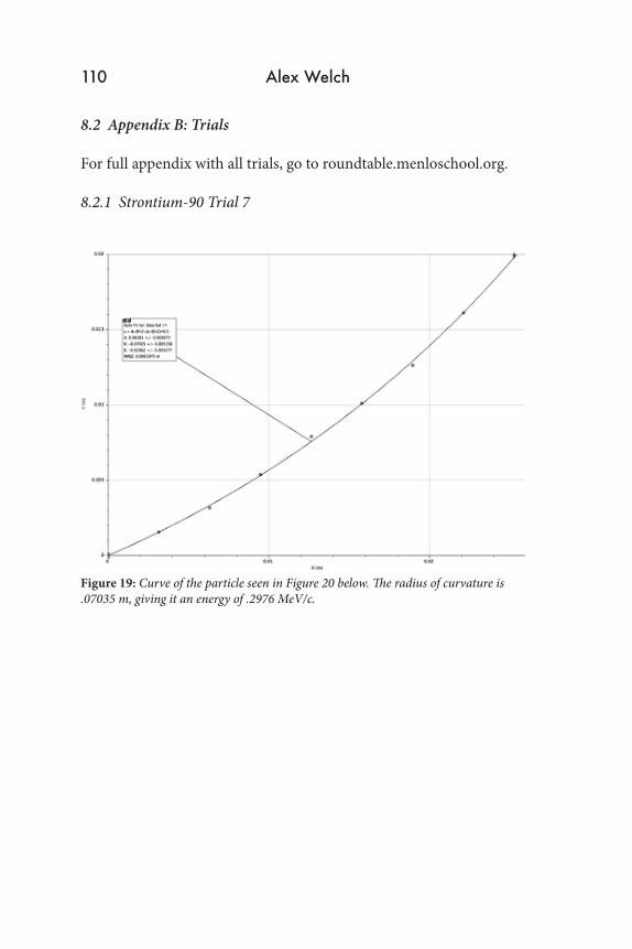
8.2.1 Strontium-90 Trial 7

Figure 19: Curve of the particle seen in Figure 20 below. The radius of curvature is .07035 m, giving it an energy of .2976 MeV/c.

110 Alex Welch


Figure 20: Photograph taken of a beta particle emitted from Strontium-90 in Trial 7 of experiment

112 Alex Welch

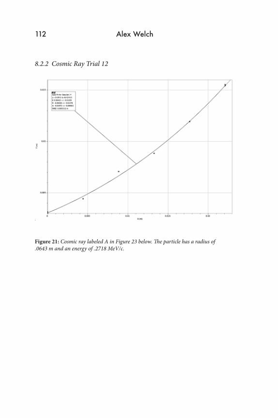
8.2.2 Cosmic Ray Trial 12

Figure 21: Cosmic ray labeled A in Figure 23 below. The particle has a radius of .0643 m and an energy of .2718 MeV/c.


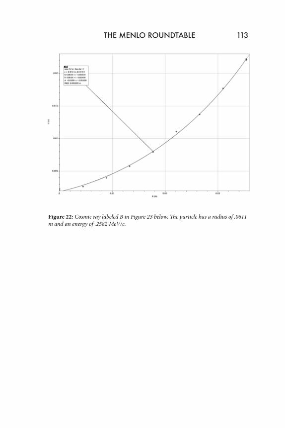
Figure 22: Cosmic ray labeled B in Figure 23 below. The particle has a radius of .0611 m and an energy of .2582 MeV/c.

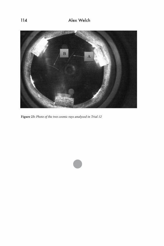
Figure 23: Photo of the two cosmic rays analyzed in Trial 12

114 Alex Welch

diffusion cloud chamber

Documents