Diffusion limited aggregation simulations of Saffman-Taylor instability for Newtonian and Non-Newtonian fluids

Timothy Barnes, Scott Lieberman, Stephanie Maruca

A Hele-Shaw cell contains two plates, held at constant, small, distance from one another. A fluid, Fluid 2, is sandwiched between the plates. Another fluid, Fluid 1, is injected into Fluid 2. The boundary between the two fluids in unstable; this is called Saffman-Taylor instability.

Figure 1: Hele-Shaw Cell

Saffman-Taylor instability in a Hele-Shaw cell can be modeled using Monte Carlo Methods.

When two Newtonian fluids are used, the system can be modeled using Laplace’s Equation, ∇!𝑃 = 0, when P is pressure. This model is derived using the geometry of the cell, Euler’s equation, Navier-Stokes Equation, and Darcy’s Law. Monte-Carlo Methods can be used to solve Laplace’s equation. To apply a Monte-Carlo Method, the geometry must be broken into a grid. At a boundary grid point, the average is the number of points earned at that boundary. For example, consider the following grid:

𝑅 𝐴 =14 𝑅 𝐵 + 𝑅 𝐶 + 𝑅 𝐷 + 𝑅 𝐸        𝑖𝑛𝑡𝑒𝑟𝑖𝑜𝑟  𝑝𝑜𝑖𝑛𝑡

𝑅 𝐷 = 𝑔        𝑏𝑜𝑢𝑛𝑑𝑎𝑟𝑦  𝑝𝑜𝑖𝑛𝑡   If a walker is started at Point A, it will move randomly throughout the grid. If it lands on an interior grid point, it will be assigned a value of the sum of the probability of moving to the four spaces around it divided by one-fourth. When it lands on a boundary point, it will earn the value of that boundary and then be terminated; in the above example, it will earn a value of g at the left boundary and a value of zero at any other boundary. [1]

g A

B

C

D

E

This method works for solving Laplace’s equation for a Hele-Shaw Cell. Diffusion

limited aggregation simulations are based on Monte Carlo simulations.   This can be done by defining a boundary around a selected region. To solve this boundary value problem, define a Green’s function,  

i𝑔 𝑟, 𝑠 = 0, where r can move about the region and the boundary and s always lies on the boundary and

i𝑓 𝑥,𝑦 = 4𝑓 𝑥,𝑦 − 𝑓 𝑥 + 1,𝑦 − 𝑓 𝑥 − 1,𝑦 − 𝑓 𝑥,𝑦 + 1 − 𝑓(𝑥,𝑦 − 1). g is zero when r is on the boundary, unless r is equal to s, then

𝑔 = 1. This Green’s function can be used to solve Laplace’s equation:

𝑝 𝑟 = 𝑔(𝑟 , 𝑠)𝜓(𝑠), summed over the boundary, where ψ is the potential. g is the solution to Laplace’s equation in for a Hele-Shaw cell.[2]

This can also be explained using finite differences. Assume Δ is sufficiently small, then

∇!𝑃 =𝑃 𝑥 + ∆,𝑦 + 𝑃 𝑥 − ∆,𝑦 + 𝑃 𝑥,𝑦 + ∆ + 𝑃 𝑥,𝑦 − ∆ − 4 𝑥,𝑦

∆! = 0.

Consider a grid with spacing Δ, the probability of a walker moving to a neighboring space is ¼. At a boundary point, the walker is terminated and a value is calculated for P:

𝑃 𝑥!,𝑦! = 𝑓 𝑥!,𝑦! . The values of many walkers can be used to find the solution to Laplace’s Equation,

𝑃 𝑥,𝑦 ≈1𝑁 𝑓 𝑥!!,𝑦!! ,

!

where N is the number of walkers.[3] To apply the Monte-Carlo Method to this system, a circular area is broken down into a grid.

A “seed” is placed in the center of the circle. Each grid space unoccupied by the seed is given a value of zero. Each grid space occupied by the seed is given a value of one. A number of “walker” were placed randomly on the circle surrounding the seed. The circle must have a large radius to mimic the walkers coming in to the seed from infinity. Each walker moves randomly, either up, down, left or right. Each direction is equally probable. When the walker hits the seed, there is a probability it will “stick” to the seed. If it sticks, the space is given a value of one and it becomes part of the seed. The probability of the walker sticking depends on the local curvature of the seed,

𝑃 𝑁! = 𝐴 !!!!− !!!

!!+ 𝐵.

When A is equivalent to surface tension, and B is an adjustable parameter.[2] The growing seed is model of Fluid 1 as it is injected into Fluid 2.

Figure 2:

Monte-Carlo Simulation of a Hele-Shaw Cell with Newtonian Fluids without Hole Filling

This method leaves the possibility for holes to form in the simulation. A solution to fill these holes is to move the walkers into the holes as they are created. Meaning that if a walker reaches a grid point with a value of one, it scans the area for spaces where holes are forming, and move into the spaces. This is accomplished by allowing a walker than has already “stuck” to move into the neighboring grid space that has a lower potential (the grid space with the highest number of surrounding spaces with a value of one). This process creates a more realistic simulation (see Figure 3).

Figure 3:

Monte Carlo Simulation of a Hele-Shaw Cell with Newtonian Fluids with Hole Filling

Multiple simulations were run with different parameter. A parameter equivalent to surface tension, A, was varied from 1 to 10. The space between the fingers, λ, was calculated for each of these simulations. This value was calculated by drawing circles of different radii around the center of the simulation; the number of fingers passing through the circle was counted and divided by the radius of the circle. The relationship between these values should be a square root function according a linear stability analysis of the problem. This relationship is seen in the demonstrations (see Figure 4).

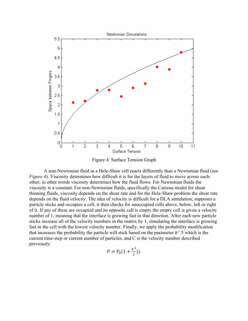
Figure 4: Surface Tension Graph

A non-Newtonian fluid in a Hele-Shaw cell reacts differently than a Newtonian fluid (see Figure 4). Viscosity determines how difficult it is for the layers of fluid to move across each-other; in other words viscosity determines how the fluid flows. For Newtonian fluids the viscosity is a constant. For non-Newtonian fluids, specifically the Carreau model for shear thinning fluids, viscosity depends on the shear rate and for the Hele-Shaw problem the shear rate depends on the fluid velocity. The idea of velocity is difficult for a DLA simulation; supposes a particle sticks and occupies a cell, it then checks for unoccupied cells above, below, left or right of it. If any of these are occupied and its opposite cell is empty the empty cell is given a velocity number of 1, meaning that the interface is growing fast in that direction. After each new particle sticks increase all of the velocity numbers in the matrix by 1, simulating the interface is growing fast in the cell with the lowest velocity number. Finally, we apply the probability modification that increases the probability the particle will stick based on the parameter 𝑘^.5 which is the current time-step or current number of particles, and C is the velocity number described previously:

𝑃 = 𝑃!(1+! .!

!)).

Figure 5: Monte Carlo Simulation of a Hele-Shaw Cell with Non-Newtonian Fluid with Hole Filling

Figure 6: Experimental Setup

Experiments were completed using a Hele-Shaw Cell with different gap widths and different solutions. An optical table was used (see Figure 6). Four stand bars where secured in the table, so they could hold up the cell. A white piece of paper with a needle sized hole in the

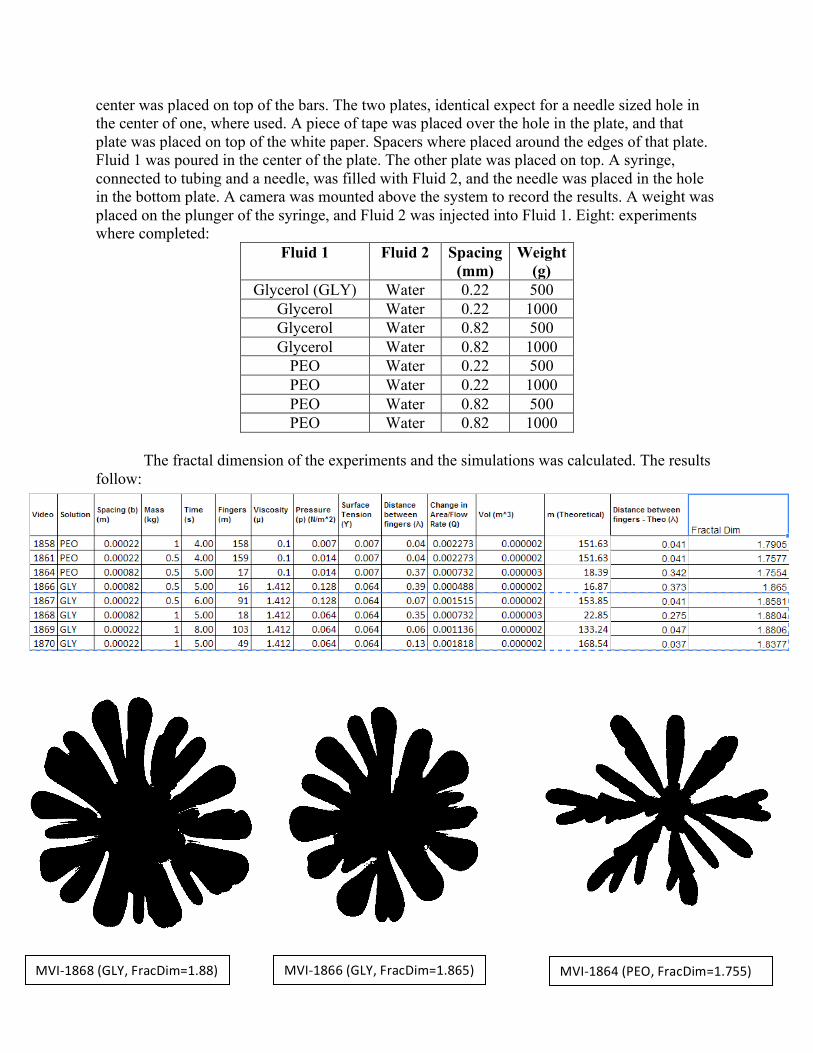
center was placed on top of the bars. The two plates, identical expect for a needle sized hole in the center of one, where used. A piece of tape was placed over the hole in the plate, and that plate was placed on top of the white paper. Spacers where placed around the edges of that plate. Fluid 1 was poured in the center of the plate. The other plate was placed on top. A syringe, connected to tubing and a needle, was filled with Fluid 2, and the needle was placed in the hole in the bottom plate. A camera was mounted above the system to record the results. A weight was placed on the plunger of the syringe, and Fluid 2 was injected into Fluid 1. Eight: experiments where completed:

Fluid 1 Fluid 2 Spacing (mm)

Weight (g)

Glycerol (GLY) Water 0.22 500 Glycerol Water 0.22 1000 Glycerol Water 0.82 500 Glycerol Water 0.82 1000

PEO Water 0.22 500 PEO Water 0.22 1000 PEO Water 0.82 500 PEO Water 0.82 1000

The fractal dimension of the experiments and the simulations was calculated. The results follow:

MVI-­‐1868  (GLY,  FracDim=1.88)   MVI-­‐1866  (GLY,  FracDim=1.865)   MVI-­‐1864  (PEO,  FracDim=1.755)  

Videos of the experiments were analyzed using image processing software and converted

to binary, as seen above. The fractal dimensions are listed below the images (FracDim). There was a definite trend in the data seen above: the Newtonian (glycerol) experiments had fractal dimension in the range of 1.8377-1.8806. The Non-Newtonian (PEO) experiments had fractal dimensions in the range 1.7554-1.7905. Clearly, the Non-Newtonian Experiments had a smaller fractal dimension than the Newtonian Experiments. In the final two images above, the Non-Newtonian simulation and the Newtonian simulation, we see a similar trend; the Non-Newtonian simulation had a fractal dimension of 1.6895 and the Newtonian Simulation had a fractal dimension of 1.7933. Even though these fractal dimensions do not match those of the experiments, we see the same trend—the Non-Newtonian results have a smaller fractal dimension than the Newtonian results.

There was error in the experiments that may have contributed to the larger fractal dimensions than the simulations. Low contrast between the paper and fluid made image-processing difficult. Also, the fluid had a tendency to pool where it was injected, instead of the immediate fingering from the center as seen in the simulation results. This would increase the fractal dimension, as the larger center would make the fluid take on a shape more like that of a disk (which has fractal dimension 2). Air bubbles also complicated analysis of the fractal dimension.

The results of the Newtonian simulations, linear stability analysis and the experiments display similarities in trends as surface tension is increased and fractal dimension. The Non-Newtonian results and experiments do not display similarities in fractal dimension. Further research must be done to find a suitable sticking rule for Non-Newtonian Fluids in the Hele-Shaw cell.

MVI-­‐1858  (PEO,  FracDim=1.79)  

Non-­‐Newtonian  Simulation  

FracDim=1.6895  

Newtonian  Simulation  

FracDim=1.7933  

Works Cited

[1] Farlow, Stanley J. (1993), Partial Differential Equations for Scientists and Engineers, Dover Books on Mathematics [2] Kadanoff, Leo P. (1985), Simulating Hydrodynamics: a Pedestrian Model, Journal of Statistieal Physics [3] Landau, David P. (2005), A Guide to Monte Carlo Simulations in Statistical Physics, Cambridge University Press