diffusion monte carlo - istituto nazionale di fisica...
TRANSCRIPT

Diffusion Monte Carlo
Stefano Gandolfi
Los Alamos National Laboratory (LANL)
Microscopic Theories of Nuclear Structure, Dynamics andElectroweak Currents
June 12-30, 2017, ECT*, Trento, Italy
Stefano Gandolfi (LANL) - [email protected] Diffusion Monte Carlo 1 / 19

Diffusion Monte Carlo
The variational wave function can be very accurate, but things can beimproved.
The time-dependent Schroedinger equation is (~ = 1)
−i ∂∂t
Ψ(R, t) = H Ψ(R, t)
and its solution is given by:
Ψ(R, t) = e−i H (t−t0)Ψ(R, t0)
we will call τ = it imaginary time.
Stefano Gandolfi (LANL) - [email protected] Diffusion Monte Carlo 2 / 19

Diffusion Monte Carlo
Projection in imaginary time:
Let’s assume that the wave function can be expanded over a set ofeigenstates of the Hamiltonian H:
ψ =∑n
φn
Then let’s apply the evolution operator exp[−(H − ET )τ ]:
e−(H−ET )τψ = e−(H−ET )τ∑n
φn
=∑n
e−(En−ET )τφn → c0φ0
In this way, in the limit of τ →∞ we can extract the ground-state of H.
Note: ET is a constant to guarantee a finite normalization.
Stefano Gandolfi (LANL) - [email protected] Diffusion Monte Carlo 3 / 19

Diffusion Monte Carlo
Let’s represent the wave function as an ensemble of points, i.e. walkers inthe volume:
〈R|ΨT 〉 =∑n
cnδ(R − Rn)
then:
〈R ′|ΨT (τ)〉 =
∫dR G (R,R ′, τ)〈R|ΨT (0)〉
where G (R,R ′, τ) is the propagator of the Hamiltonian, and we haveused the identity
1 =
∫dR |R〉〈R|
Stefano Gandolfi (LANL) - [email protected] Diffusion Monte Carlo 4 / 19

Diffusion Monte Carlo
Let’s define the propagator in coordinates as the matrix element betweentwo points in the volume:
G (R,R ′, τ) = 〈R|e−(H−ET )τ |R ′〉
The expression above is very difficult to calculate. What easy instead is:
G (R,R ′, t) ≈N∏n
G (Rn,Rn−1, δτ) ≈[〈R|e−Tδτe−V δτeET δτ |R ′〉
]nwhere δτ = τ/N, and 〈R|e−Tδτe−V δτ |R ′〉 is easy to sample.
Then we need to iterate the integral in previous slide many times toreach the limit τ →∞.
Stefano Gandolfi (LANL) - [email protected] Diffusion Monte Carlo 5 / 19

Diffusion Monte Carlo
The kinetic energy is sampled as a diffusion of particles (in 3D):
〈R ′|e− ~2
2m∇2δτ |R〉 =
( m
2π~2δτ
)3A/2
e−m(R−R′)2/2~2δτ
= G0(R,R ′, δτ)
Note: G0 is normalized!
The (scalar, local) potential and ET give the weight of the configuration:
〈R ′|e−V δτeET δτ |R〉 = wδR,R′
Note: the weight w is basically the normalization of exp[−V (R)δτ ], asthe propagator is dependent to the “arrival” (or “starting”) point in thediffusion: ∫
dR G (R,R ′, δτ) = e−V (R′)δτ
Stefano Gandolfi (LANL) - [email protected] Diffusion Monte Carlo 6 / 19
Diffusion Monte Carlo
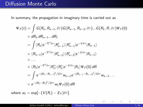
In summary, the propagation in imaginary time is carried out as
ΨT (t) =
∫G (Rn,Rn−1, δτ)G (Rn−1,Rn−2, δτ)...G (R1,R, δτ)ΨT (0)
× dRn dRn−1...dR1
=
∫〈Rn|e−∇
2δτ |R ′n−1〉〈R ′n−1|e−V δτ |Rn−1〉
× 〈Rn−1|e−∇2δτ |R ′n−2〉〈R ′n−2|e−V δτ |Rn−2〉
× . . .
× 〈R2|e−∇2δτ |R ′1〉〈R ′1|e−V δτ |R1〉ΨT (0) dR
=
∫e−(Rn−Rn−1)2/2δτwn−1e
−(Rn−1−Rn−2)2/2δτwn−2 . . .
× e−(R2−R1)2/2δτw1ΨT (0) dR
where wi = exp[−(V (Ri )− ET )δτ ].
Stefano Gandolfi (LANL) - [email protected] Diffusion Monte Carlo 7 / 19

Diffusion Monte Carlo
Remember that the wave function is represented as a collection ofwalkers.
In the previous expression, the product of weights can become very large(or very small) for some of them. For example, consider the case of aninfinite potential like repulsive Coulomb. If two particles are sampled tobe close, the weight becomes zero, and then that walker will alwayscontribute zero to the observables.
Stefano Gandolfi (LANL) - [email protected] Diffusion Monte Carlo 8 / 19
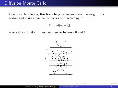
Diffusion Monte Carlo
One possible solution, the branching technique: take the weight of awalker and make a number of copies of it according to:
# = int[wi + ξ]
where ξ is a (uniform) random number between 0 and 1.
Stefano Gandolfi (LANL) - [email protected] Diffusion Monte Carlo 9 / 19

Importance sampling
The sampling of G (R,R ′, δτ) can be very noisy. Assume that we know awave function ΨG that describes reasonably the system (i.e. in most ofthe cases the variational wave function). Then, it is very efficient to“project” our sampling over the “good guess”:
〈ΨG |R ′〉〈R ′|ΨT (τ)〉 =
∫dR G (R,R ′, τ)〈ΨG |R ′〉〈R|ΨT (0)〉
=
∫dR G (R,R ′, τ)
〈ΨG |R ′〉〈ΨG |R〉
〈ΨG |R〉〈R|ΨT (0)〉
= f (R ′, τ)
In this way we are sampling a different distribution f (R ′, τ) whosevariance is much improved from before!
Stefano Gandolfi (LANL) - [email protected] Diffusion Monte Carlo 10 / 19

Importance sampling
Let’s see how to sample the quantity G (R,R ′, τ) 〈R′|ΨG 〉〈R|ΨG 〉 (notation
ΨG (R) = 〈R|ΨG 〉).
The first thing to note is that the normalization of the modifiedpropagator is now dependent to the “arrival” point in the diffusion.
Before:
N(R ′) =
∫dR G (R,R ′, δτ) = e−[V (R′)−ET ]δτ
Now:
N(R ′) =
∫dR G (R,R ′, δτ)
ΨG (R ′)
ΨG (R)
Stefano Gandolfi (LANL) - [email protected] Diffusion Monte Carlo 11 / 19

Importance sampling
In the limit of small δτ (small |R − R ′|) we can expand
Ψ∗G (R)
Ψ∗G (R)
ΨG (R ′)
ΨG (R)≈1 +
Ψ∗G (R)
Ψ∗G (R)
1
ΨG (R)
∂
∂xiΨG (R) (xi − x ′i )
+1
2
Ψ∗G (R)
Ψ∗G (R)ΨG (R)
∂2
∂xi∂xjΨG (R) (xi − x ′i )(xj − x ′j ) + . . .
And we can prove that
N(R ′) = e−[
Ψ∗G (R)HΨG (R′)Ψ∗G
(R)ΨG (R′) −ET ]δτ
At the same time, the modified propagator can be sampled as a shiftedGaussian
exp
[−m(R − R ′)2
2~2δτ
]−→ exp
−m(R − R ′ +
Ψ∗G (R)∇ΨG (R)Ψ∗G (R)ΨG (R)
)2
2~2δτ
Note: there are other ways to sample the modified propagator.
Stefano Gandolfi (LANL) - [email protected] Diffusion Monte Carlo 12 / 19
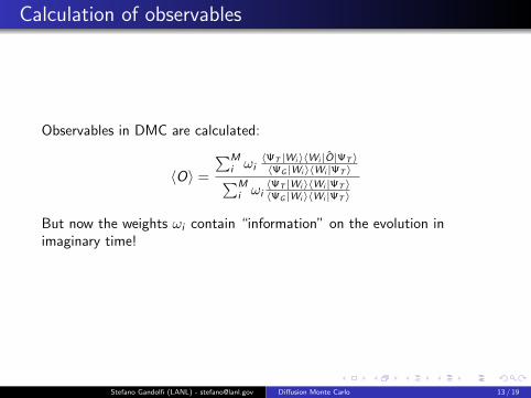
Calculation of observables
Observables in DMC are calculated:
〈O〉 =
∑Mi ωi
〈ΨT |Wi 〉〈Wi |O|ΨT 〉〈ΨG |Wi 〉〈Wi |ΨT 〉∑M
i ωi〈ΨT |Wi 〉〈Wi |ΨT 〉〈ΨG |Wi 〉〈Wi |ΨT 〉
But now the weights ωi contain “information” on the evolution inimaginary time!
Stefano Gandolfi (LANL) - [email protected] Diffusion Monte Carlo 13 / 19

Diffusion Monte Carlo
The DMC algorithm can be summarized in the following steps:
1 Generate a set of N walkers randomly or distributed with VMC
2 Loop over the N walkers, and for each i-th walker:
3 Make a step: R ′i = Ri + ~2δτm
Ψ∗T (R)∇ΨG (R)ΨT (R)ΨG (R) + ξ
√~2δτ/m
4 Calculate the weight: wi = exp[−(
ΨT (R)HΨG (R′)ΨT (R)ΨG (R′) − ET
)δτ]
5 Do branching
6 Increase the total imaginary-time by a unit of δτ
7 Iterate with 2) until the equilibration is reached, then resetestimators and iterate until the error is small enough
Stefano Gandolfi (LANL) - [email protected] Diffusion Monte Carlo 14 / 19

DMC: the first piece of code
Note: here we assume that ΨG = ΨT !
...
do j=1,nstep
nw=0
do n=1,nwalk
xtest=xold(n)-sigma**2*alpha*xold(n)+sigma*rgauss(irn)
eloc=-0.5_r8*((alpha*xtest)**2-alpha)+0.5_r8*omega**2*xtest**2
weight=exp(-dt*(eloc-etrial))
call ran(csi,irn)
iwt=weight+csi
do k=1,iwt
nw=nw+1
xnew(nw)=xtest
enddo
tau=tau+dt
enddo
enddo
...
Stefano Gandolfi (LANL) - [email protected] Diffusion Monte Carlo 15 / 19

Diffusion Monte Carlo
An example: 1D harmonic oscillator, projection in imaginary time.Energy as a function of the imaginary time τ :
0 1 2 3 4 5
τ [ω-1
]
0.49
0.5
0.51
0.52
0.53
0.54E
[ω
]
1D harmonic oscillator
Ground-state resolved!
Stefano Gandolfi (LANL) - [email protected] Diffusion Monte Carlo 16 / 19

Growth energy
In DMC a very nice “diagnostic tool” is the growth energy. It can becalculated by measuring the weights of the walkers.
If we had the exact wave function and ET the exact energy, then theweight of each walker would be 1 independently to the configuration (i.e.HΨ/Ψ = ET ). Then, by averaging over weights, we can define:
ωi = exp[−(E i
G − ET )δτ]
and we get:
〈EG 〉 = ET −1
δτlog (〈ω〉)
Note: EG is very similar to the local energy if δτ is small enough!
Exercise: test it.
Stefano Gandolfi (LANL) - [email protected] Diffusion Monte Carlo 17 / 19

Mixed estimates
Note that in DMC we calculate “mixed estimates”, i.e.:
〈O〉mix = 〈ΨT |O|Φ0〉
where ΨT is the variational wave function, and Φ0 is the DMC (groundstate) one. By assuming that
|ΨT 〉 ' |Φ0〉+ λ|δΨ〉
it is easy to show that
〈O〉 = 〈Φ0|O|Φ0〉 ' 2〈O〉mix − 〈O〉vmc
where 〈O〉vmc = 〈ΨT |O|ΨT 〉.
Exercise: prove that.
Note: the only exceptions where 〈O〉mix is truly the ground state one isfor those operators for which [H,O] = 0. Can you guess why?
Stefano Gandolfi (LANL) - [email protected] Diffusion Monte Carlo 18 / 19

Diffusion Monte Carlo
DMC is a tool to calculate the energy of a many-body system for a givenwave function by projecting it in imaginary time.
... for now :-)
Stefano Gandolfi (LANL) - [email protected] Diffusion Monte Carlo 19 / 19
Diffusion Monte Carlo
DMC is a tool to calculate the energy of a many-body system for a givenwave function by projecting it in imaginary time.
... for now :-)
Stefano Gandolfi (LANL) - [email protected] Diffusion Monte Carlo 19 / 19