digital coherent receivers and advanced optical modulation ...€¦ · advanced optical modulation...
TRANSCRIPT
Advanced Communication Systems course, Technology and Communications Systems Master (ETSIT-UPM), Final Work 2014
Abstract—Recent advances in coherent optical receivers is
reviewed. Digital-Signal-Processing (DSP) based phase and
polarization management techniques make coherent detection
robust and feasible. With coherent detection, the complex field of
the received optical signal is fully recovered, allowing
compensation of linear and nonlinear optical impairments
including chromatic dispersion (CD) and polarization-mode
dispersion (PMD) using digital filters. Coherent detection and
advanced optical modulation formats have become a key
ingredient to the design of modern dense wavelength-division
multiplexed (DWDM) optical broadband networks. In this paper,
firstly we present the different subsystems of a digital coherent
optical receiver, and secondly, we will compare the performance
of some multi-level and multi-dimensional modulation formats in
some physical impairments and in high spectral-efficiency (SE)
and high-capacity DWDM transmissions, simulating the DSP
with Matlab and the optical network performance with
OptiSystem software.
Index Terms—Coherent Detection, DWDM, polarization
multiplexing, modulation formats, optical impairments.
I. INTRODUCTION
HE amount of traffic carried on backbone networks has
been growing exponentially over the past two decades, at
about 30 to 60% per year, depending on the nature and
penetration of services offered by various network operators in
different geographic regions [74], [9]. The increasing number
of applications relying on machine-to-machine traffic and
cloud computing could accelerate this growth the required
network bandwidth for such applications may scale with data
processing capabilities, at close to 90% per year [45]. Non-
cacheable real-time multi-media applications will also drive
the need for more network bandwidth.
The demand for communication bandwidth has been
economically met by wavelength-division multiplexed
(WDM) optical transmission systems, researched, developed,
A.Macho ( ) Departamento de Tecnología Fotónica y Bioingeniería
Escuela Técnica Superior de Ingenieros de Telecomunicación Universidad
Politécnica de Madrid, Avda. Complutense nº30
28040 Madrid, Spain
e-mail: [email protected]
telephone: +34649994228
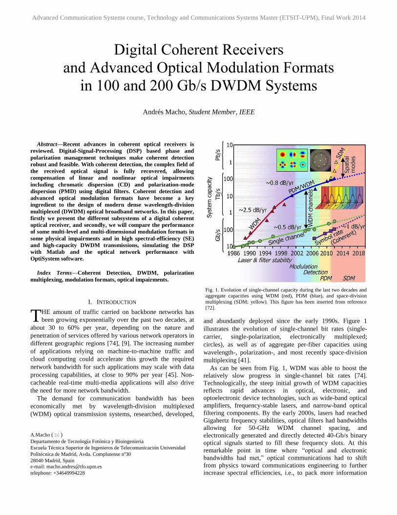
and abundantly deployed since the early 1990s. Figure 1
illustrates the evolution of single-channel bit rates (single-
carrier, single-polarization, electronically multiplexed;
circles), as well as of aggregate per-fiber capacities using
wavelength-, polarization-, and most recently space-division
multiplexing [41].
As can be seen from Fig. 1, WDM was able to boost the
relatively slow progress in single-channel bit rates [74].
Technologically, the steep initial growth of WDM capacities
reflects rapid advances in optical, electronic, and
optoelectronic device technologies, such as wide-band optical
amplifiers, frequency-stable lasers, and narrow-band optical
filtering components. By the early 2000s, lasers had reached
Gigahertz frequency stabilities, optical filters had bandwidths
allowing for 50-GHz WDM channel spacing, and
electronically generated and directly detected 40-Gb/s binary
optical signals started to fill these frequency slots. At this
remarkable point in time where “optical and electronic
bandwidths had met,” optical communications had to shift
from physics toward communications engineering to further
increase spectral efficiencies, i.e., to pack more information
Digital Coherent Receivers
and Advanced Optical Modulation Formats
in 100 and 200 Gb/s DWDM Systems
Andrés Macho, Student Member, IEEE
T
Fig. 1. Evolution of single-channel capacity during the last two decades and aggregate capacities using WDM (red), PDM (blue), and space-division
multiplexing (SDM; yellow). This figure has been inserted from reference
[72].
Advanced Communication Systems course, Technology and Communications Systems Master (ETSIT-UPM), Final Work 2014
into the limited ( -THz) bandwidth of the commercially most
attractive class of single-band (C- or L-band) optical
amplifiers. Consequently, by 2002 high-speed fiber-optic
systems research had started to investigate new modulation
formats using direct detection.
With the drive towards per-channel bit rates of 100 Gb/s in
2005 [69], however, it became clear that additional techniques
were needed if 100-Gb/s channels were to be used on the by
then widely established 50-GHz WDM infrastructure,
supporting a spectral efficiency of 2 b/s/Hz [70], [75]. In this
context, polarization-division multiplexed (PDM) allowed for
a reduction of symbol rates, which brought 40 and 100-Gb/s
optical signals.
At this point coherent optical receivers emerged as the main
area of interest in broadband optical communications due to
the high receiver sensitivities which they can achieve. They
have since been combined with digital post-processing to
perform all-electronic CD and PMD compensation, frequency-
and phase locking, and polarization demultiplexing. The use
of coherent optical receivers with the combination of
advanced modulation formats has led to increase the long
transmission distances and high spectral efficiencies required
for the current commercial core optical networks.
In this paper, we discuss the operation of digital coherent
optical receivers considering each of the subsystems required
and we analyze higher-order coherent optical modulation
formats as the underlying technology that has fueled capacity
growth over the past years. The paper is organized as follows.
Section II focuses in the basics of coherent receiver structure
and DSP algorithms for CD and PMD equalization, and phase
recovery of the two main modulation formats employed in
high-capacity DWDM networks: PDM-QPSK and PDM-
16QAM. Section III reviews the main advanced modulation
formats, analyzes their tolerance to some physical
impairments and presents three high SE DWDM
transmissions. Finally, in Section IV the paper concludes with
a discussion of the main results obtained in this work.
II. SUBSYSTEMS OF A DIGITAL COHERENT RECEIVER AND
DIGITAL-SIGNAL-PROCESSING
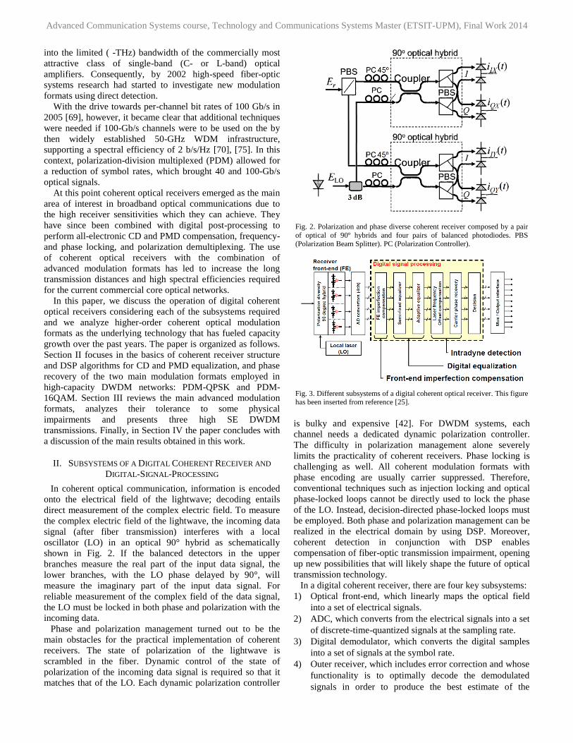
In coherent optical communication, information is encoded
onto the electrical field of the lightwave; decoding entails
direct measurement of the complex electric field. To measure
the complex electric field of the lightwave, the incoming data
signal (after fiber transmission) interferes with a local
oscillator (LO) in an optical 90° hybrid as schematically
shown in Fig. 2. If the balanced detectors in the upper
branches measure the real part of the input data signal, the
lower branches, with the LO phase delayed by 90°, will
measure the imaginary part of the input data signal. For
reliable measurement of the complex field of the data signal,
the LO must be locked in both phase and polarization with the
incoming data.
Phase and polarization management turned out to be the
main obstacles for the practical implementation of coherent
receivers. The state of polarization of the lightwave is
scrambled in the fiber. Dynamic control of the state of
polarization of the incoming data signal is required so that it
matches that of the LO. Each dynamic polarization controller
is bulky and expensive [42]. For DWDM systems, each
channel needs a dedicated dynamic polarization controller.
The difficulty in polarization management alone severely
limits the practicality of coherent receivers. Phase locking is
challenging as well. All coherent modulation formats with
phase encoding are usually carrier suppressed. Therefore,
conventional techniques such as injection locking and optical
phase-locked loops cannot be directly used to lock the phase
of the LO. Instead, decision-directed phase-locked loops must
be employed. Both phase and polarization management can be
realized in the electrical domain by using DSP. Moreover,
coherent detection in conjunction with DSP enables
compensation of fiber-optic transmission impairment, opening
up new possibilities that will likely shape the future of optical
transmission technology.
In a digital coherent receiver, there are four key subsystems:
1) Optical front-end, which linearly maps the optical field
into a set of electrical signals.
2) ADC, which converts from the electrical signals into a set
of discrete-time-quantized signals at the sampling rate.
3) Digital demodulator, which converts the digital samples
into a set of signals at the symbol rate.
4) Outer receiver, which includes error correction and whose
functionality is to optimally decode the demodulated
signals in order to produce the best estimate of the
Fig. 2. Polarization and phase diverse coherent receiver composed by a pair
of optical of 90º hybrids and four pairs of balanced photodiodes. PBS (Polarization Beam Splitter). PC (Polarization Controller).
Fig. 3. Different subsystems of a digital coherent optical receiver. This figure has been inserted from reference [25].
Advanced Communication Systems course, Technology and Communications Systems Master (ETSIT-UPM), Final Work 2014
sequence of bits, which were encoded by the transmitter.
We shall focus on the first three of these subsystems, which
form the inner receiver, whose functionality is to produce a
“synchronized channel,” which is as close as possible to the
information theoretic communication channel.
In order to discuss the DSP contained in the digital
demodulator, we begin by considering the structural level
design of the DSP, as can be seen in Fig. 3. While for a
particular digital coherent receiver, the subsystems employed
may differ slightly from those detailed in Fig. 3, they give
some indication as to the design choices, which can be made
at a structural level, such as the ordering of the subsystems.
Additional considerations at the structural level include the
combining or partitioning of subsystems, for example, the
carrier phase estimation may be separated into estimating the
frequency offset and the residual carrier phase. It is possible to
perform joint carrier phase and symbol synchronization [31].
We shall focus on the structural and algorithmic level rather
than the implementation level, where the finite resources, such
as machine precision and clock speed are considered. In order
to discuss performance of the digital coherent receiver at the
algorithmic level, we will restrict our discussion to one
possible realization, where the subsystems are arranged, as in
Fig. 3, including the “inner receiver” and the “outer receiver,”
which performs symbol estimation and decoding.
There are numerous feedback paths between the subsystems.
Some of these paths occur naturally, such as between the
phase estimation subsystem and frequency estimation
subsystem, however, other paths depend on the algorithms
employed. For example, feedback from the symbol estimation
and decoding subsystem is required for data-aided algorithms,
but not for blind algorithms. Likewise, for synchronous
sampling at the baud rate, feedback would be required from
the timing-recovery subsystem to the ADC subsystem, which
could be omitted for asynchronous sampling. In the
subsequent sections of this paper, we shall discuss each of
these subsystems independently, forming a basis for
understanding the operation of a digital coherent receiver
employing feedback between the subsystems.
A. Phase and Polarization Diverse Coherent Optical
Receiver
The functionality of the optical front-end, being both phase
and polarization diverse, is to linearly map the incoming
optical field into the electrical domain. To realize this
functionality, the architecture is shown in Fig. 2, is often
employed, which employs a pair of 90º hybrids, one for each
polarization [42]. The received signal interferes inside an
optical hybrid with a LO-signal provided by another CW-laser
converting both quadratures of X-and Y-polarization into the
electrical domain. Both the LO- and transmitter laser have
phase noise, which can be modeled as a random walk process
of the variance 𝜎2 = 2𝜋 ∙ ∆𝜗 ∙ 𝑑𝑡 with ∆𝜗 representing the
laser linewidth and 𝑑𝑡 is the time between two observations.
Typical laser linewidths range from ~100 kHz, corresponding
to commercially available external cavity lasers (ECL), up to a
few MHz for a conventional DFB laser. The LO-laser is
usually free running within ~1 GHz of the optical frequency of
the transmit laser, which is referred to as intradyne detection.
In this case, the remaining frequency offset is compensated
digitally, e.g., by applying a higher-order nonlinearity to the
signal and estimating the offset from the spectrum.
A four port phase- and polarization-diversity hybrid may be
used with single-ended detection, resulting in the four
photocurrents given in (1):
[ 𝑖𝐼𝑋(𝑡)𝑖𝑄𝑋(𝑡)
𝑖𝐼𝑌(𝑡)
𝑖𝑄𝑌(𝑡)]
~
[ 𝑅𝑒{𝐸𝑋𝐸𝐿𝑂
∗ } +1
2|𝐸𝑋|
2 +1
4|𝐸𝐿𝑂|
2
𝐼𝑚{𝐸𝑋𝐸𝐿𝑂∗ } +
1
2|𝐸𝑋|
2 +1
4|𝐸𝐿𝑂|
2
𝑅𝑒{𝐸𝑌𝐸𝐿𝑂∗ } +
1
2|𝐸𝑌|
2 +1
4|𝐸𝐿𝑂|
2
𝐼𝑚{𝐸𝑌𝐸𝐿𝑂∗ } +
1
2|𝐸𝑌|
2 +1
4|𝐸𝐿𝑂|
2]
(1)
Each of the photocurrents consists of three terms: a coherent
detection term (leftmost), a signal complex envelope term
(center), and an LO complex envelope term (rightmost).
Although the LO complex envelope term is constant (and may
therefore be removed with AC coupling), the signal complex
envelope is time varying and must be minimized relative to
the coherent detection term by making the LO much more
powerful than the signal.
To overcome the constraints imposed on signal-LO power
ratios, balanced photo-detection is often employed for
coherent optical receivers. In this scenario, an 8 port optical
hybrid is used, with a 180º phase shift between each
quadrature pair. The pairs of outputs are then differentially
amplified to eliminate the direct-detection components in the
signal. The eight output ports of the hybrid are given by:
[ 𝑖𝐼𝑋+(𝑡)
𝑖𝐼𝑋−(𝑡)
𝑖𝑄𝑋+(𝑡)
𝑖𝑄𝑋−(𝑡)
𝑖𝐼𝑌+(𝑡)
𝑖𝐼𝑌−(𝑡)
𝑖𝑄𝑌+(𝑡)
𝑖𝑄𝑌−(𝑡)]
~
[ 1
2𝑅𝑒{𝐸𝑋𝐸𝐿𝑂
∗ } +1
4|𝐸𝑋|
2 +1
8|𝐸𝐿𝑂|
2
−1
2𝑅𝑒{𝐸𝑋𝐸𝐿𝑂
∗ } +1
4|𝐸𝑋|
2 +1
8|𝐸𝐿𝑂|
2
1
2𝐼𝑚{𝐸𝑋𝐸𝐿𝑂
∗ } +1
4|𝐸𝑋|
2 +1
8|𝐸𝐿𝑂|
2
−1
2𝐼𝑚{𝐸𝑋𝐸𝐿𝑂
∗ } +1
4|𝐸𝑋|
2 +1
8|𝐸𝐿𝑂|
2
1
2𝑅𝑒{𝐸𝑌𝐸𝐿𝑂
∗ } +1
4|𝐸𝑌|
2 +1
8|𝐸𝐿𝑂|
2
−1
2𝑅𝑒{𝐸𝑌𝐸𝐿𝑂
∗ } +1
4|𝐸𝑌|
2 +1
8|𝐸𝐿𝑂|
2
1
2𝐼𝑚{𝐸𝑌𝐸𝐿𝑂
∗ } +1
4|𝐸𝑌|
2 +1
8|𝐸𝐿𝑂|
2
−1
2𝐼𝑚{𝐸𝑌𝐸𝐿𝑂
∗ } +1
4|𝐸𝑌|
2 +1
8|𝐸𝐿𝑂|
2]
(2)
After differential amplification, this becomes the four-
dimensional signal given by:
[ 𝑖𝐼𝑋(𝑡)𝑖𝑄𝑋(𝑡)
𝑖𝐼𝑌(𝑡)
𝑖𝑄𝑌(𝑡)]
~
[ 𝑅𝑒{𝐸𝑋𝐸𝐿𝑂
∗ }
𝐼𝑚{𝐸𝑋𝐸𝐿𝑂∗ }
𝑅𝑒{𝐸𝑌𝐸𝐿𝑂∗ }
𝐼𝑚{𝐸𝑌𝐸𝐿𝑂∗ }]
(3)
Advanced Communication Systems course, Technology and Communications Systems Master (ETSIT-UPM), Final Work 2014
The received signal defined by (3) represents the ideal
coherently received optical field, which is: no direct-detection
terms, infinite common-mode rejection between differential
pairs and perfectly matched optical path lengths in the hybrid
resulting in an exact 90º difference between quadratures.
Ideally, the I and the Q channels of a quadrature
communication system are orthogonal to each other. However,
implementation imperfections (e.g., incorrect bias points
settings for the I, Q, and phase ports, imperfect splitting ratio
of couplers, photodiodes responsivity mismatch, and
misadjustment of the polarization controllers) can create
amplitude and phase imbalances that destroy the orthogonality
between the two received channels and degrade performance
of the quadrature system. Also, in practice, phase diversity
receivers are vulnerable to imperfections in the optical 90º
hybrid, which result in dc offsets and both amplitude and
phase errors in the received signals. These effects give rise to
quadrature imbalance in a communication system.
All of these imperfections, can in principle, be compensated
digitally, thereby relaxing the requirements on the optical
components. While blind source separation techniques, such
as independent component analysis could be used [25], it is
often possible to simplify this problem, reducing it to finding
two pairs of mutually orthogonal components 𝐸𝑥𝐼 , 𝐸𝑦
𝐼 , 𝐸𝑥𝑄 , 𝐸𝑦
𝑄.
In the field of DSP, there are numerous techniques to achieve
this for creating orthogonal components, such as the Gram–
Schmidt orthogonalization algorithm (see subsection II.C).
B. Analog-to-Digital Conversion
Having mapped the signal from the optical domain into the
electrical domain, the next stage is to convert the analog
signals into a set of digital signals. From a functional view, we
can consider the ADC to be made up of two subsystems, a
sampler, which samples the signal in time, converting the
continuous time analog signal into a discrete-time analog
signal, followed by a quantizer, which converts the discrete-
time analog signal into a finite set of values determined by the
bits of resolution in the ADC.
For a digital communication system, which transmits
symbols at a rate of Rs symbols per second, the minimum
sampling rate is Rs (in hertz). In general, however, for
asynchronous sampling a sampling rate of 2·Rs Hz, is
advantageous, giving rise to two samples per symbol, thereby
enabling digital timing recovery. While in practice, there may
be a slight difference between clocks of the transmitter and the
receiver, the signal may be resampled by interpolating of the
digital signal, which will be discussed in subsection II.F.
The receive-side ADC, usually specified in terms of its
effective number of bits (ENoB). As shown in [65], the
required ADC resolution at a 1-dB receiver sensitivity penalty
and at a pre-FEC bit error ratio (BER) typical of coded
systems (e.g., is approximately 3 bits more than what would
be needed to recover the √𝑀 amplitude levels of the two
signal quadratures if the constellation were received without
any distortions and phase rotations. The technological trade-
off between ADC resolution and bandwidth is analyzed in a
series of papers by Walden [56], [57], and reveals a reduction
of about 3.3 ENoB per decade of analog input bandwidth.
C. Orthogonalization: front-end imperfection compensation
The functionality of this subsystem is to recover the
orthogonality between the I and Q components in each
polarization transmitted. Ideally, the I and the Q channels of a
quadrature communication system are orthogonal to each
other.
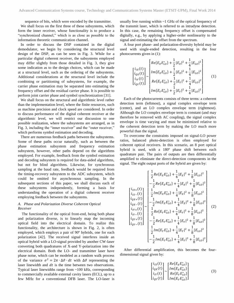
However, as we can see in Fig. 4 (constellations simulated
with OptiSystem) the main optical impairments (chromatic
dispersion, polarization-mode dispersion and fiber Kerr
nonlinearities) and hardware imperfections (e.g., incorrect bias
points settings for the I, Q, and phase ports, imperfect splitting
ratio of couplers, photodiodes responsivity mismatch, and
misadjustment of the polarization controllers) can create
amplitude and phase imbalances that destroy the orthogonality
between the two received channels and degrade performance
of the multilevel modulation formats. Also, in practice, phase
diversity receivers are vulnerable to imperfections in the
optical 90º hybrid, which result in dc offsets and both
amplitude and phase errors in the received signals. These
effects give rise to quadrature imbalance in a digital
communication system.
The Gram–Schmidt orthogonalization procedure (GSOP)
enables a set of nonorthogonal samples to be transformed into
a set of orthogonal samples. Given two nonorthogonal
components of the received signal, denoted by 𝑟𝐼(𝑡) and 𝑟𝑄(𝑡),
the GSOP results in a new pair of orthonormal signals,
denoted by 𝐼0(𝑡) and 𝑄0(𝑡), as follows:
Fig. 4. (a) QPSK constellation imbalanced due to the photodiodes responsivity mismatch at the quadrature receiver structure. (b) I and Q
channels imbalanced in a homodyne receiver due to misalignment between
the axes of the two PBS inside of the quadrature receiver. (c) I and Q channels imbalanced in a heterodyne receiver due to misalignment between
the axes of the two PBS inside of the quadrature receiver. (d) Correction of
nonorthogonality in the above case using GSOP in OptiSystem.
Advanced Communication Systems course, Technology and Communications Systems Master (ETSIT-UPM), Final Work 2014
𝐼0(𝑡) =𝑟𝐼(𝑡)
√𝑃𝐼 (4)
𝑄′(𝑡) = 𝑟𝑄(𝑡) −𝜌 ∙ 𝑟𝐼(𝑡)
𝑃𝐼 (5)
𝑄0(𝑡) =𝑄′(𝑡)
√𝑃𝑄 (6)
Where 𝜌 = 𝐸{𝑟𝐼(𝑡) ∙ 𝑟𝑄(𝑡)} is the correlation coefficient,
𝑃𝐼 = 𝐸{𝑟𝐼2(𝑡)}, 𝑃𝑄 = 𝐸{𝑟𝑄
2(𝑡)}. Fig. 4(c)-(d) shows an
example where de GSOP has been applied to a nonorthogonal
set of data with quadrature imbalance and an intermediate
frequency (IF) of 100 MHz. The GSOP corrects the mismatch
and transforms the ellipse into a circle, with the thickness
determined by the amount of noise. The orthogonality for
received signals with quadrature imbalance can thus be
restored using (4)–(6) with the amplitudes of the recovered
signals normalized correctly [34].
D. Fixed Equalization
The main driver for coherent optical communication is the
possibility to compensate for transmission impairments by
using DSP. This is possible only when both the phase and the
magnitude of the complex field of light are detected. All linear
impairments in fiber-optic transmission systems can
potentially be compensated, in particular GVD and PMD.
While in principle equalization could be realized in one
subsystem, it is generally beneficial to partition the problem
into static and dynamic equalization.
GVD compensation requires static equalization with large
static filters. In contrast, dynamic equalization requires
adaptive equalization with a set of relatively short adaptive
filters to compensate the rotation of the state-of-polarization
(SOP) of the signal, which is essential to polarization
demultiplexing and to compensate de PMD effects.
D.1 GVD compensation
Dispersion in optical fiber is an all-pass filter on the electric
field of the lightwave, given by a complex transfer function in
the frequency domain [61], [70], [41, Ch. 5]:
𝐻𝑓(𝜔) ≈ 𝑒𝑥𝑝 {+𝑗𝐷 ∙ 𝐿 ∙ 𝜆0
2
4𝜋𝑐0𝜔2 − 𝑗
𝑆 ∙ 𝐿 ∙ 𝜆04
24𝜋2𝑐02 𝜔3} (7)
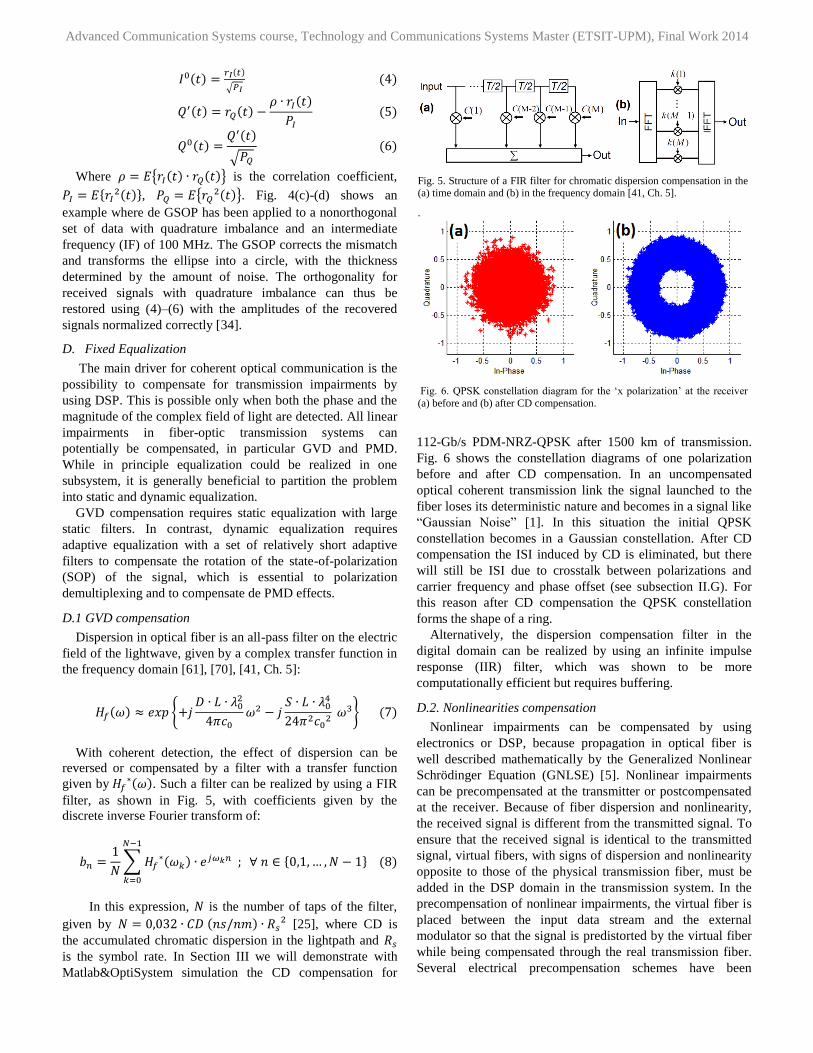
With coherent detection, the effect of dispersion can be
reversed or compensated by a filter with a transfer function
given by 𝐻𝑓∗(𝜔). Such a filter can be realized by using a FIR
filter, as shown in Fig. 5, with coefficients given by the
discrete inverse Fourier transform of:
𝑏𝑛 =1
𝑁∑𝐻𝑓
∗(𝜔𝑘)
𝑁−1
𝑘=0
∙ 𝑒𝑗𝜔𝑘𝑛 ; ∀ 𝑛 ∈ {0,1, … , 𝑁 − 1} (8)
In this expression, 𝑁 is the number of taps of the filter,
given by 𝑁 = 0,032 ∙ 𝐶𝐷 (𝑛𝑠/𝑛𝑚) ∙ 𝑅𝑠2 [25], where CD is
the accumulated chromatic dispersion in the lightpath and 𝑅𝑠 is the symbol rate. In Section III we will demonstrate with
Matlab&OptiSystem simulation the CD compensation for
112-Gb/s PDM-NRZ-QPSK after 1500 km of transmission.
Fig. 6 shows the constellation diagrams of one polarization
before and after CD compensation. In an uncompensated
optical coherent transmission link the signal launched to the
fiber loses its deterministic nature and becomes in a signal like
“Gaussian Noise” [1]. In this situation the initial QPSK
constellation becomes in a Gaussian constellation. After CD
compensation the ISI induced by CD is eliminated, but there
will still be ISI due to crosstalk between polarizations and
carrier frequency and phase offset (see subsection II.G). For
this reason after CD compensation the QPSK constellation
forms the shape of a ring.
Alternatively, the dispersion compensation filter in the
digital domain can be realized by using an infinite impulse
response (IIR) filter, which was shown to be more
computationally efficient but requires buffering.
D.2. Nonlinearities compensation
Nonlinear impairments can be compensated by using
electronics or DSP, because propagation in optical fiber is
well described mathematically by the Generalized Nonlinear
Schrödinger Equation (GNLSE) [5]. Nonlinear impairments
can be precompensated at the transmitter or postcompensated
at the receiver. Because of fiber dispersion and nonlinearity,
the received signal is different from the transmitted signal. To
ensure that the received signal is identical to the transmitted
signal, virtual fibers, with signs of dispersion and nonlinearity
opposite to those of the physical transmission fiber, must be
added in the DSP domain in the transmission system. In the
precompensation of nonlinear impairments, the virtual fiber is
placed between the input data stream and the external
modulator so that the signal is predistorted by the virtual fiber
while being compensated through the real transmission fiber.
Several electrical precompensation schemes have been
Fig. 5. Structure of a FIR filter for chromatic dispersion compensation in the time domain [Kaminow13, Ch. 5].
.
Fig. 6. QPSK constellation diagram for the ‘x polarization’ at the receiver
(a) before and (b) after CD compensation.
Fig. 5. Structure of a FIR filter for chromatic dispersion compensation in the (a) time domain and (b) in the frequency domain [41, Ch. 5].
.
Fig. 6. QPSK constellation diagram for the ‘x polarization’ at the receiver
(a) before and (b) after CD compensation.
Advanced Communication Systems course, Technology and Communications Systems Master (ETSIT-UPM), Final Work 2014
demonstrated to compensate for chromatic dispersion or
nonlinearity in single-channel or WDM systems [48], [42],
[24]. In the postcompensation of nonlinear impairments, the
virtual fiber is placed after coherent detection so that the
signal is distorted in the real transmission fiber while being
compensated through the virtual fiber. Postcompensation
using coherent detection and DSP has been shown to be very
effective in chromatic dispersion compensation and
intrachannel nonlinearity compensation [42].
While the complexity may be reduced using wavelets [26],
nonlinear compensation based on one step per span may still
be prohibitive to implement in hardware. Nevertheless, it
provides a benchmark against which simpler compensation
schemes may be compared, such as the three block models
Hammerstein–Wiener (NLN), the Wiener-Hammerstein
(LNL) [18], with the challenge being to improve the nonlinear
tolerance of the system without making the DSP prohibitive to
implement.
E. Adaptive Equalization
The purpose of this subsystem is to compensate the PMD
degradation and to eliminate the crosstalk between the two
polarizations of the received PDM signal. This crosstalk arises
due to the misalignment between the SOP of the received
signal and the axes of the initial PBS in Fig. 2. The key is to
observe the analogy between dual-polarization optical systems
and multiple-input–multiple-output (MIMO) radiofrequency
wireless communications. As a result, algorithms for wireless
MIMO channel estimation can be readily applied to
polarization demultiplexing in optical polarization MIMO [7].
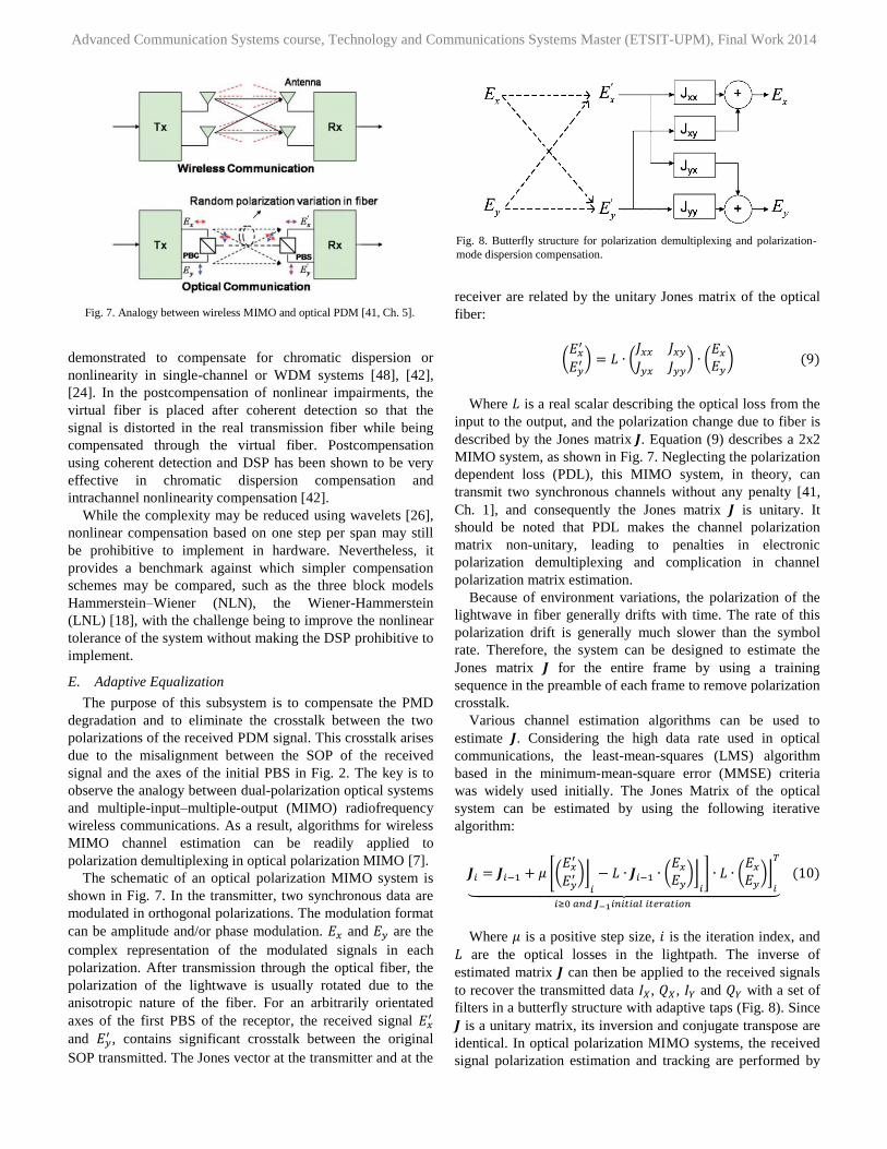
The schematic of an optical polarization MIMO system is
shown in Fig. 7. In the transmitter, two synchronous data are
modulated in orthogonal polarizations. The modulation format
can be amplitude and/or phase modulation. 𝐸𝑥 and 𝐸𝑦 are the
complex representation of the modulated signals in each
polarization. After transmission through the optical fiber, the
polarization of the lightwave is usually rotated due to the
anisotropic nature of the fiber. For an arbitrarily orientated
axes of the first PBS of the receptor, the received signal 𝐸𝑥′
and 𝐸𝑦′ , contains significant crosstalk between the original
SOP transmitted. The Jones vector at the transmitter and at the
receiver are related by the unitary Jones matrix of the optical
fiber:
(𝐸𝑥′
𝐸𝑦′ ) = 𝐿 ∙ (
𝐽𝑥𝑥 𝐽𝑥𝑦𝐽𝑦𝑥 𝐽𝑦𝑦
) ∙ (𝐸𝑥𝐸𝑦) (9)
Where 𝐿 is a real scalar describing the optical loss from the
input to the output, and the polarization change due to fiber is
described by the Jones matrix 𝑱. Equation (9) describes a 2x2
MIMO system, as shown in Fig. 7. Neglecting the polarization
dependent loss (PDL), this MIMO system, in theory, can
transmit two synchronous channels without any penalty [41,
Ch. 1], and consequently the Jones matrix 𝑱 is unitary. It
should be noted that PDL makes the channel polarization
matrix non-unitary, leading to penalties in electronic
polarization demultiplexing and complication in channel
polarization matrix estimation.
Because of environment variations, the polarization of the
lightwave in fiber generally drifts with time. The rate of this
polarization drift is generally much slower than the symbol
rate. Therefore, the system can be designed to estimate the
Jones matrix 𝑱 for the entire frame by using a training
sequence in the preamble of each frame to remove polarization
crosstalk.
Various channel estimation algorithms can be used to
estimate 𝑱. Considering the high data rate used in optical
communications, the least-mean-squares (LMS) algorithm
based in the minimum-mean-square error (MMSE) criteria
was widely used initially. The Jones Matrix of the optical
system can be estimated by using the following iterative
algorithm:
𝑱𝑖 = 𝑱𝑖−1 + 𝜇 [(𝐸𝑥′
𝐸𝑦′ )⌋
𝑖
− 𝐿 ∙ 𝑱𝑖−1 ∙ (𝐸𝑥𝐸𝑦)⌋𝑖
] ∙ 𝐿 ∙ (𝐸𝑥𝐸𝑦)⌋𝑖
𝑇
⏟ 𝑖≥0 𝑎𝑛𝑑 𝑱−1𝑖𝑛𝑖𝑡𝑖𝑎𝑙 𝑖𝑡𝑒𝑟𝑎𝑡𝑖𝑜𝑛
(10)
Where 𝜇 is a positive step size, 𝑖 is the iteration index, and
𝐿 are the optical losses in the lightpath. The inverse of
estimated matrix 𝑱 can then be applied to the received signals
to recover the transmitted data 𝐼𝑋, 𝑄𝑋, 𝐼𝑌 and 𝑄𝑌 with a set of
filters in a butterfly structure with adaptive taps (Fig. 8). Since
𝑱 is a unitary matrix, its inversion and conjugate transpose are
identical. In optical polarization MIMO systems, the received
signal polarization estimation and tracking are performed by
Fig. 7. Analogy between wireless MIMO and optical PDM [41, Ch. 5].
Fig. 8. Butterfly structure for polarization demultiplexing and polarization-
mode dispersion compensation.
Advanced Communication Systems course, Technology and Communications Systems Master (ETSIT-UPM), Final Work 2014
DSP algorithms, and no optical dynamic polarization control
is required at the receiver.
However, it is possible to estimate the Jones matrix of the
optical channel without relying on a training sequence if there
exist statistical properties of the transmitted symbols that can
be exploited. In particular, for PDM systems using constant-
intensity modulation formats such as M-(D)PSK, the Jones
matrix can be estimated using the fact that the modulus of the
received signal should be constant [3]. Without loss of
generality, let us assume that the constant modulus is unity.
An estimate of the Jones matrix is obtained by minimizing the
mean squared errors ⟨휀𝑥,𝑦2 ⟩ of the quantities 휀𝑥,𝑦 = 1 −
|𝐸′𝑥,𝑦|2. In order to do so, the gradient of the mean squared
error with respect to the appropriate elements of the Jones
matrix should vanish, i.e.:
𝜕휀𝑥2
𝜕𝐽𝑥𝑥= 0,
𝜕휀𝑥2
𝜕𝐽𝑥𝑦= 0,
𝜕휀𝑦2
𝜕𝐽𝑦𝑥= 0,
𝜕휀𝑦2
𝜕𝐽𝑦𝑦= 0 (11)
To obtain the estimate of the channel Jones matrix, it is
initialized as an identity matrix. Subsequently, the matrix
elements are updated by using the stochastic gradient
algorithm of [16] as follows:
𝐽𝑥𝑥 ⟶ 𝐽𝑥𝑥 + 𝛿 ∙ 휀𝑥 ∙ 𝐸𝑥 ∙ 𝐸𝑥′ ∗ (12)
𝐽𝑥𝑦 ⟶ 𝐽𝑥𝑦 + 𝛿 ∙ 휀𝑥 ∙ 𝐸𝑥 ∙ 𝐸𝑦′ ∗ (13)
𝐽𝑦𝑥 ⟶ 𝐽𝑦𝑥 + 𝛿 ∙ 휀𝑦 ∙ 𝐸𝑦 ∙ 𝐸𝑥′ ∗ (14)
𝐽𝑦𝑦 ⟶ 𝐽𝑦𝑦 + 𝛿 ∙ 휀𝑦 ∙ 𝐸𝑦 ∙ 𝐸𝑦′ ∗ (15)
Where * denotes complex conjugate, (𝐸𝑥 , 𝐸𝑦) is the
demultiplexed optical field and 𝛿 is the positive convergence
parameter. This algorithm is known as Constant Modulus
Algorithm (CMA). The CMA was proposed by Godard in
[16], as a means of blind equalization for QPSK signals in the
1980s. In M-QAM systems it is found that the classic CMA
becomes much less effective and therefore can no longer be
used as a stand-alone equalization algorithm. This is because
an M-QAM signal does not present constant symbol
amplitude. As a result, the CMA error signal will not approach
zero even for an ideal M-QAM signal, resulting in extra noise
after equalization. To address this issue, we can use in the
DSP the multi-modulus algorithm (CMMA). Due to the limit
extension of this work we cannot go into details, but the reader
can obtain more information in [75].
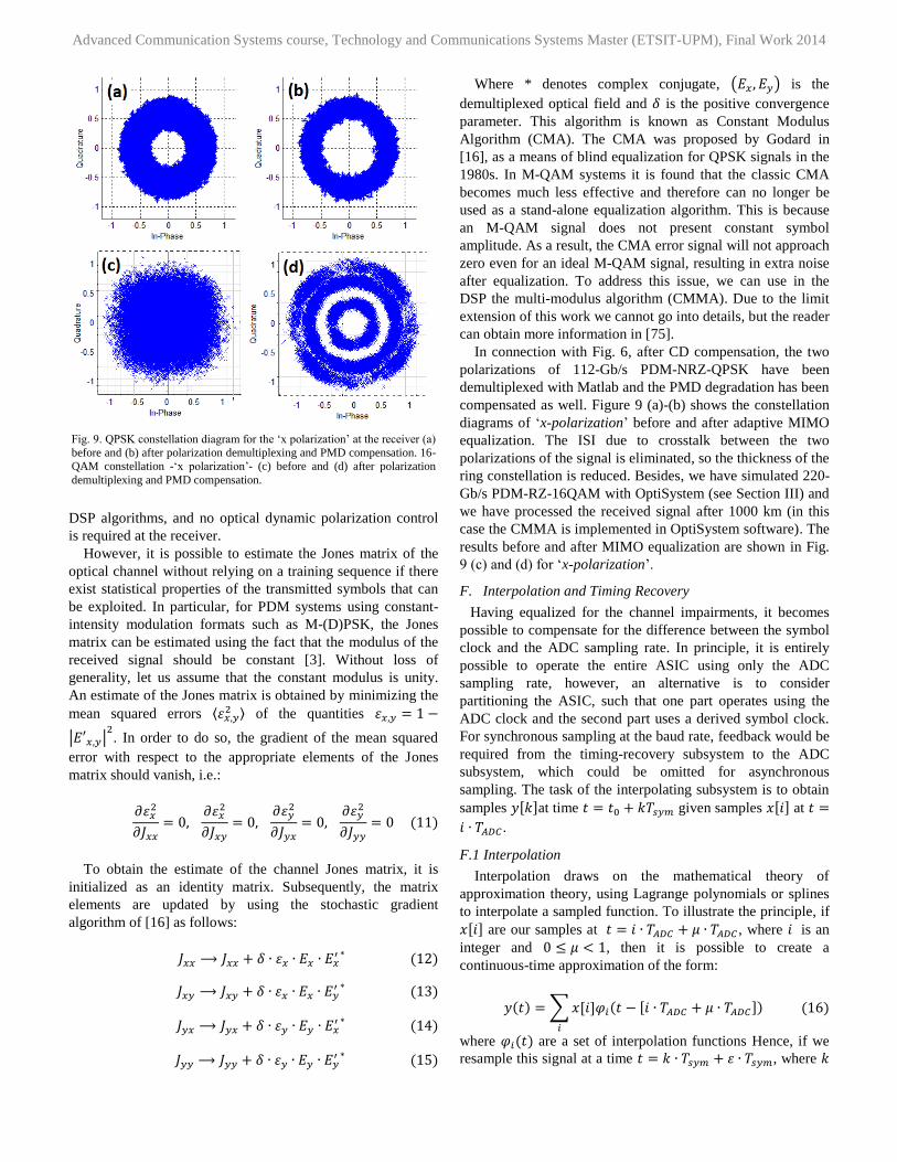
In connection with Fig. 6, after CD compensation, the two
polarizations of 112-Gb/s PDM-NRZ-QPSK have been
demultiplexed with Matlab and the PMD degradation has been
compensated as well. Figure 9 (a)-(b) shows the constellation
diagrams of ‘x-polarization’ before and after adaptive MIMO
equalization. The ISI due to crosstalk between the two
polarizations of the signal is eliminated, so the thickness of the
ring constellation is reduced. Besides, we have simulated 220-
Gb/s PDM-RZ-16QAM with OptiSystem (see Section III) and
we have processed the received signal after 1000 km (in this
case the CMMA is implemented in OptiSystem software). The
results before and after MIMO equalization are shown in Fig.
9 (c) and (d) for ‘x-polarization’.
F. Interpolation and Timing Recovery
Having equalized for the channel impairments, it becomes
possible to compensate for the difference between the symbol
clock and the ADC sampling rate. In principle, it is entirely
possible to operate the entire ASIC using only the ADC
sampling rate, however, an alternative is to consider
partitioning the ASIC, such that one part operates using the
ADC clock and the second part uses a derived symbol clock.
For synchronous sampling at the baud rate, feedback would be
required from the timing-recovery subsystem to the ADC
subsystem, which could be omitted for asynchronous
sampling. The task of the interpolating subsystem is to obtain
samples 𝑦[𝑘]at time 𝑡 = 𝑡0 + 𝑘𝑇𝑠𝑦𝑚 given samples 𝑥[𝑖] at 𝑡 =
𝑖 ∙ 𝑇𝐴𝐷𝐶 .
F.1 Interpolation
Interpolation draws on the mathematical theory of
approximation theory, using Lagrange polynomials or splines
to interpolate a sampled function. To illustrate the principle, if
𝑥[𝑖] are our samples at 𝑡 = 𝑖 ∙ 𝑇𝐴𝐷𝐶 + 𝜇 ∙ 𝑇𝐴𝐷𝐶 , where 𝑖 is an
integer and 0 ≤ 𝜇 < 1, then it is possible to create a
continuous-time approximation of the form:
𝑦(𝑡) = ∑𝑥[𝑖]𝜑𝑖(𝑡 − [𝑖 ∙ 𝑇𝐴𝐷𝐶 + 𝜇 ∙ 𝑇𝐴𝐷𝐶])
𝑖
(16)
where 𝜑𝑖(𝑡) are a set of interpolation functions Hence, if we
resample this signal at a time 𝑡 = 𝑘 ∙ 𝑇𝑠𝑦𝑚 + 휀 ∙ 𝑇𝑠𝑦𝑚, where 𝑘
Fig. 9. QPSK constellation diagram for the ‘x polarization’ at the receiver (a)
before and (b) after polarization demultiplexing and PMD compensation. 16-
QAM constellation -‘x polarization’- (c) before and (d) after polarization
demultiplexing and PMD compensation.
Advanced Communication Systems course, Technology and Communications Systems Master (ETSIT-UPM), Final Work 2014
is an integer and 0 ≤ 휀 < 1, then the samples 𝑦[𝑘] will be
given by:
𝑦[𝑘] = ∑𝑥[𝑖]𝜑𝑖(𝑘𝑇𝑠𝑦𝑚 + 휀𝑇𝑠𝑦𝑚 − [𝑖𝑇𝐴𝐷𝐶 + 𝜇𝑇𝐴𝐷𝐶])
𝑖
(17)
such that the output is a linear combination of the inputs, and
hence, may be realized as an FIR filter. For the case of linear
interpolation, the samples 𝑦[𝑘] will be a linear combination of
𝑥[𝑖] and 𝑥[𝑖 + 1]. Linear interpolation forms the basis of
higher order approximations, such as cubic interpolation or
step interpolation. Nevertheless, as the degree of the
approximation is increased, it does not necessarily follow that
the quality of the approximation improves, indicating that step
interpolation outperforms linear or cubic interpolation [23],
[44], [58].
F.2 Timing Recovery
The timing recovery has been a topic of extensive research
[31] with both non-data-aided and data-aided [37] algorithms
being employed. One such algorithm aims to maximize the
squared modulus |𝑦(𝑚𝑘, 𝜇𝑘)|2 of the interpolated signal
𝑦[𝑘] = 𝑦(𝑚𝑘, 𝜇𝑘) [31]. Differentiating |𝑦(𝑚𝑘 , 𝜇𝑘)|2 with
respect to time gives the error signal as follows:
𝑒(𝑚𝑘) =𝑑
𝑑𝑡(|𝑦(𝑚𝑘, 𝜇𝑘)|
2)
≈ 2𝑅𝑒 {𝑦(𝑚𝑘, 𝜇𝑘)[𝑦(𝑚𝑘 + 1, 𝜇𝑘) − 𝑦(𝑚𝑘 − 1, 𝜇𝑘)]
2𝑇𝑠𝑦𝑚} (18)
with this error signal going to zero when the signal is
synchronized. We may use this error signal 𝑒(𝑚𝑘) to update
𝑤𝑘, our estimate of 𝑇𝑠𝑦𝑚/𝑇𝐴𝐷𝐶 , such that:
𝑤𝑘+1 = 𝑤𝑘 +∑ 𝑐[𝑖] ∙
𝑁−1
𝑖=0
𝑒(𝑚𝑘−𝑖) (19)
where the error signal is filtered by an FIR filter of length N with coefficients 𝑐[𝑖], which incorporate the convergence
factor for this stochastic gradient method.
G. Carrier Frequency and Phase Estimation
Given the structural design of the DSP, we have elected to
separate the bulk frequency estimation from the carrier
recovery. We can model the received signal such a:
𝑥𝑖𝑛[𝑘] = 𝑥𝑠𝑦𝑚[𝑘]𝑒𝑥𝑝 (𝑗(𝜃𝑠[𝑘] + 𝜃𝑒[𝑘] + 2𝜋∆𝑓 ∙ 𝑘 ∙ 𝑇𝑠𝑦𝑚)) (20)
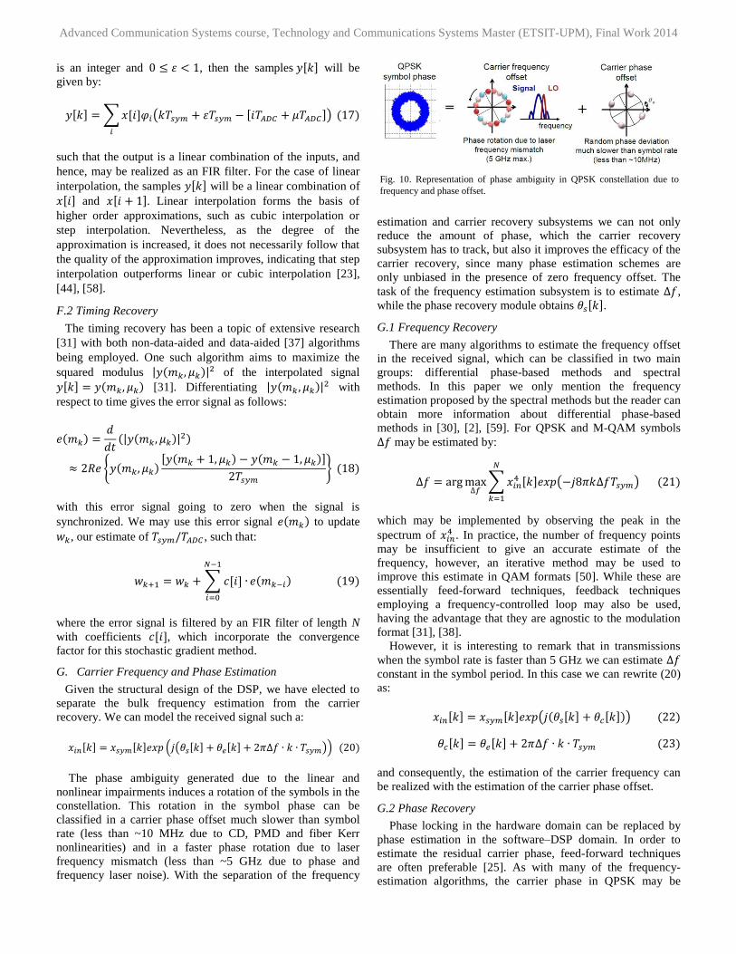
The phase ambiguity generated due to the linear and
nonlinear impairments induces a rotation of the symbols in the
constellation. This rotation in the symbol phase can be
classified in a carrier phase offset much slower than symbol
rate (less than ~10 MHz due to CD, PMD and fiber Kerr
nonlinearities) and in a faster phase rotation due to laser
frequency mismatch (less than ~5 GHz due to phase and
frequency laser noise). With the separation of the frequency
estimation and carrier recovery subsystems we can not only
reduce the amount of phase, which the carrier recovery
subsystem has to track, but also it improves the efficacy of the
carrier recovery, since many phase estimation schemes are
only unbiased in the presence of zero frequency offset. The
task of the frequency estimation subsystem is to estimate ∆𝑓,
while the phase recovery module obtains 𝜃𝑠[𝑘].
G.1 Frequency Recovery
There are many algorithms to estimate the frequency offset
in the received signal, which can be classified in two main
groups: differential phase-based methods and spectral
methods. In this paper we only mention the frequency
estimation proposed by the spectral methods but the reader can
obtain more information about differential phase-based
methods in [30], [2], [59]. For QPSK and M-QAM symbols
∆𝑓 may be estimated by:
∆𝑓 = argmax∆𝑓
∑𝑥𝑖𝑛4 [𝑘]𝑒𝑥𝑝(−𝑗8𝜋𝑘∆𝑓𝑇𝑠𝑦𝑚)
𝑁
𝑘=1
(21)
which may be implemented by observing the peak in the
spectrum of 𝑥𝑖𝑛4 . In practice, the number of frequency points
may be insufficient to give an accurate estimate of the
frequency, however, an iterative method may be used to
improve this estimate in QAM formats [50]. While these are
essentially feed-forward techniques, feedback techniques
employing a frequency-controlled loop may also be used,
having the advantage that they are agnostic to the modulation
format [31], [38].
However, it is interesting to remark that in transmissions
when the symbol rate is faster than 5 GHz we can estimate ∆𝑓
constant in the symbol period. In this case we can rewrite (20)
as:
𝑥𝑖𝑛[𝑘] = 𝑥𝑠𝑦𝑚[𝑘]𝑒𝑥𝑝(𝑗(𝜃𝑠[𝑘] + 𝜃𝑐[𝑘])) (22)
𝜃𝑐[𝑘] = 𝜃𝑒[𝑘] + 2𝜋∆𝑓 ∙ 𝑘 ∙ 𝑇𝑠𝑦𝑚 (23)
and consequently, the estimation of the carrier frequency can
be realized with the estimation of the carrier phase offset.
G.2 Phase Recovery
Phase locking in the hardware domain can be replaced by
phase estimation in the software–DSP domain. In order to
estimate the residual carrier phase, feed-forward techniques
are often preferable [25]. As with many of the frequency-
estimation algorithms, the carrier phase in QPSK may be
Fig. 10. Representation of phase ambiguity in QPSK constellation due to
frequency and phase offset.

Advanced Communication Systems course, Technology and Communications Systems Master (ETSIT-UPM), Final Work 2014
estimated using the fourth-power carrier phase recovery
algorithm [25] (Fig. 11). With 𝑥𝑖𝑛[𝑘] = 𝐴 ∙ 𝑒𝑥𝑝(𝑗(𝜃𝑠[𝑘] +
𝜃𝑐[𝑘])) and 𝜃𝑠[𝑘] = 0,± 𝜋/2, 𝜋 radians. To estimate the
carrier phase θc[k] by using DSP, the received signal is raised
to the fourth power as shown in Fig. 11, we obtain:
𝐴4 ∙ 𝑒𝑥𝑝(𝑗(4𝜃𝑠[𝑘] + 4𝜃𝑐[𝑘])) = 𝐴4 ∙ 𝑒𝑥𝑝(𝑗4𝜃𝑐[𝑘]) (24)
because 𝑒𝑥𝑝(𝑗4𝜃𝑠[𝑘]) = 1, i.e., the power operation strips off
the data phase. The carrier phase can then be computed and
subtracted from the phase of the received signal to recover the
data phase. Such a feed-forward phase estimation scheme
lends itself well to real-time digital implementation. Figure 11,
however, is an idealization where no additive noise is present
in the received signal. In realistic systems, the received signal
will contain noise dominated by either ASE–LO beat noise or
shot noise of the LO. In the presence of these additive noises,
digital carrier-phase estimation must be adapted to manage
these noises. The generalization of fourth-power carrier phase
recovery algorithm for QPSK signals gives the estimate of the
phase as follows [20]:
𝜙[𝑘] = 𝑎𝑟𝑔 {1
2𝑁 + 1∑ 𝑤[𝑛]𝑥𝑖𝑛
4 [𝑘 + 𝑛]
𝑁
𝑛=−𝑁
} (25)
where w[n] is a weighting function, which depends on the
ratio of the additive white Gaussian noise to the laser phase
noise. The result of the weighting function is to apply a
Wiener filter to estimate the phase noise [20], [47], which can
approach the performance of an ideal maximum a priori
(MAP) estimator of the phase. Using this approach for a 1-dB
penalty, a linewidth up to 28 MHz may be tracked for 28
GBaud PDM-QPSK [47].
As modulation formats move beyond QPSK to M-QAM,
the requirements on the laser linewidth become increasingly
stringent because the symbol period is longer for the same bit
rate and consequently more phase laser fluctuations will take
place due to spontaneous emissions [42], [55]. Later, in
section III.C we will analyze the tolerance of 100G-PDM-
QPSK and 200G-PDM-16QAM to frequency and phase laser
noise.
Nevertheless using conventional wireless approaches such
as decision-directed phase locked loops, have enabled a
linewidth of 1 MHz to be tracked digitally for 14 GBaud
PDM-16-QAM [54]. Furthermore, for differential 16-QAM
and 64-QAM, it has been shown that a digital phase-locked
loop can compensate for a residual frequency offset of 1% of
the symbol rate [33]. While the digital phase-locked loop
presents challenges for CMOS-based parallel implementation,
hardware efficient carrier-recovery schemes have also been
proposed with similar performance [65].
In addition to the errors due to the residual phase noise,
there is also the possibility of a cycle slip, which can have a
catastrophic effect on the performance. As discussed by
Taylor [47], in order to reduce the probability of a cycle slip to
that of the corrected the BER=10-18, the laser linewidth may
need to be reduced by two orders of magnitude, e.g., 600 kHz
for 28 GBaud PDM-QPSK. In order to minimize the impact of
phase ambiguity differential decoding has been proposed.
While this has the effect of increasing the BER by as much as
a factor of two, and hence, incurring a modest penalty (<1
dB), this often outweighs advantage of relaxed linewidth
requirements and simplified symbol decoding.
To close this subsection, we include in Fig.12 the
constellation diagrams of 112-Gb/s PDM-NRZ-QPSK and
220-Gb/s PDM-RZ-16QAM obtained at the output of the DSP
after a transmission of 1500 km and 1000 km, respectively (in
the former case the signal is processed with Matlab and in the
latter case with OptiSystem). We show the comparison before
and after carrier frequency and phase recovery in both cases.
H. Symbol Estimation and Decoding
Following carrier recovery, the symbols may be decided by
the outer receiver. This could take the form of a soft-decision
forward error correction (SD-FEC) using a Galois field
corresponding to the symbol alphabet, or symbol estimation
followed by hard-decision FEC (HD-FEC). In current systems,
which are based on hard decision decoding of binary data,
Fig. 11. Mth power carrier phase recovery algorithm. Symbol phase is
recovered by digital cancellation of carrier phase and frequency offset [25].
Fig. 12. QPSK constellation diagrams for the ‘x polarization’ at the receiver
(a) before and (b) after carrier frequency and phase recovery. 16-QAM
constellation -‘x polarization’- (c) before and (d) after carrier frequency and
phase recovery.
Advanced Communication Systems course, Technology and Communications Systems Master (ETSIT-UPM), Final Work 2014
symbol estimation and bit decoding is required. For
rectangular constellations, such as QAM, this may be achieved
by applying a series of decision thresholds to the in-phase and
quadrature components separately. While this corresponds to
the maximum likelihood symbol estimation for a system
limited by additive white Gaussian noise, by using
nonrectangular decision boundaries, it is possible to improve
the performance for systems limited by linear and nonlinear
optical impairments, which is a line of research for improve
the performance in superchannels transmissions [10], [41, Ch.
3].
III. ADVANCED OPTICAL MODULATION FORMATS IN 100 AND
200-Gb/s DWDM TRANSMISSIONS
Digital coherent detection technology described in the
above section allows the use of a universal receiver front-end
for different advanced optical modulation formats. It moves
the complexity of phase and polarization tracking into the
digital domain [42].
With the rapid growth of capacity demand on carrier’s
transport networks, spectrally-efficient modulation and
detection technology have become increasingly important due
to their potential to reduce cost per transmitted bit by sharing
fiber and optical components over more capacity. Modulation
and detection technologies capable of achieving even higher
SE might be needed for 100-Gb/s and above DWDM systems
[6], [10]. Therefore, high-spectral-efficiency multi-level
modulation formats have been proposed to increase spectral
utilization: PDM-QPSK, PDM-QDB, PDM-8-PSK, and PDM-
M-QAM [70], [75], [41, Ch. 7].
The question as to the ‘best’ modulation format there is no
unique answer to this question. Rather, the answer depends on
system requirements such as [41, Ch. 7], [72]: target per-
channel interface rate, available per-channel optical
bandwidth, spectral efficiency, target transmission reach,
optical networking requirements and transponder integration
and power consumption. Each of the above boundary
conditions implies a certain set of trade-offs that help to
determine the ‘best’ modulation format:
Symbol Rate vs Constellation Size: affecting to DAC and
ADC resolution, digital filters size in DSP (proportional
to Rs2 [60]) to compensate the linear and nonlinear optical
impairments and the tolerance to laser phase noise (the
higher the symbol rate the more sensitive to laser phase
noise and consequently, narrower-linewidth lasers are
required [49]).
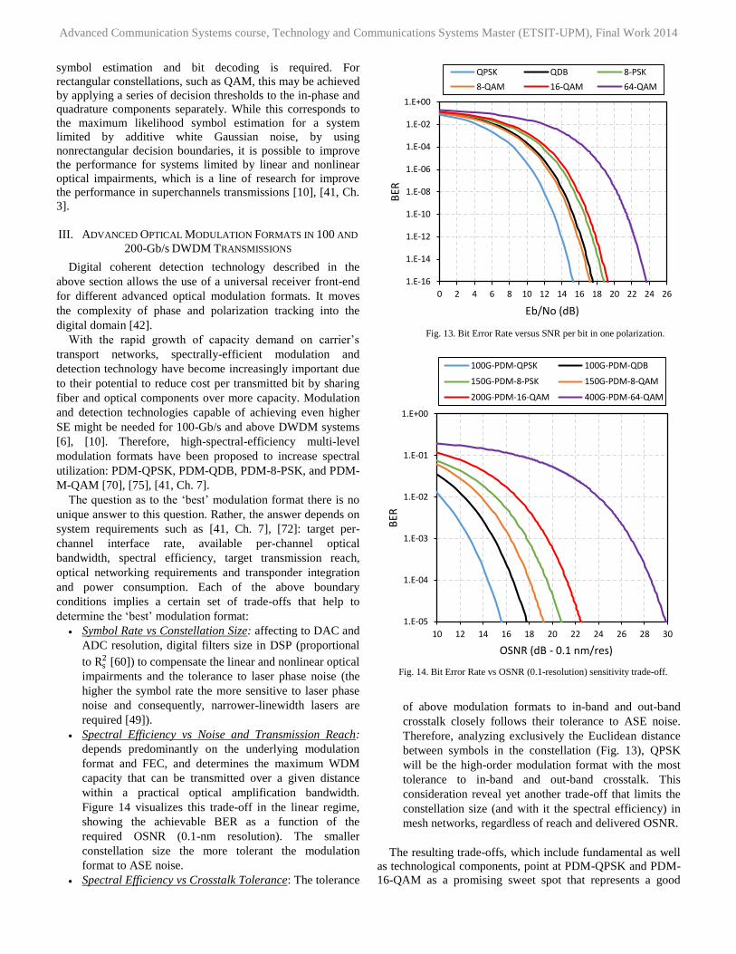
Spectral Efficiency vs Noise and Transmission Reach:
depends predominantly on the underlying modulation
format and FEC, and determines the maximum WDM
capacity that can be transmitted over a given distance
within a practical optical amplification bandwidth.
Figure 14 visualizes this trade-off in the linear regime,
showing the achievable BER as a function of the
required OSNR (0.1-nm resolution). The smaller
constellation size the more tolerant the modulation
format to ASE noise.
Spectral Efficiency vs Crosstalk Tolerance: The tolerance
of above modulation formats to in-band and out-band
crosstalk closely follows their tolerance to ASE noise.
Therefore, analyzing exclusively the Euclidean distance
between symbols in the constellation (Fig. 13), QPSK
will be the high-order modulation format with the most
tolerance to in-band and out-band crosstalk. This
consideration reveal yet another trade-off that limits the
constellation size (and with it the spectral efficiency) in
mesh networks, regardless of reach and delivered OSNR.
The resulting trade-offs, which include fundamental as well
as technological components, point at PDM-QPSK and PDM-
16-QAM as a promising sweet spot that represents a good
Fig. 13. Bit Error Rate versus SNR per bit in one polarization.
Fig. 14. Bit Error Rate vs OSNR (0.1-resolution) sensitivity trade-off.
1.E-16
1.E-14
1.E-12
1.E-10
1.E-08
1.E-06
1.E-04
1.E-02
1.E+00
0 2 4 6 8 10 12 14 16 18 20 22 24 26
BER
Eb/No (dB)
QPSK QDB 8-PSK
8-QAM 16-QAM 64-QAM
1.E-05
1.E-04
1.E-03
1.E-02
1.E-01
1.E+00
10 12 14 16 18 20 22 24 26 28 30
BER
OSNR (dB - 0.1 nm/res)
100G-PDM-QPSK 100G-PDM-QDB
150G-PDM-8-PSK 150G-PDM-8-QAM
200G-PDM-16-QAM 400G-PDM-64-QAM
Advanced Communication Systems course, Technology and Communications Systems Master (ETSIT-UPM), Final Work 2014
compromise between various limiting effects but still enables
high-performance in 100-Gb/s transmissions with PDM-QPSK
and in 200-Gb/s transmissions with PDM-16QAM. In the next
subsections we review and investigate the tolerance of 112G-
PDM-QPSK (12% overhead for FEC) and 220G-PDM-
16QAM (20% overhead for FEC) to some physical
impairments: optical filtering, crosstalk and laser phase noise.
The analysis of both formats to GVD, PMD and fiber Kerr
nonlinearities degradation remains outstanding for future
works due to space restrictions of this document. Finally, we
present three high-spectral-efficiency and high-speed DWDM
transmission experiments implementing these formats and the
optical coherent receiver presented in Section II.
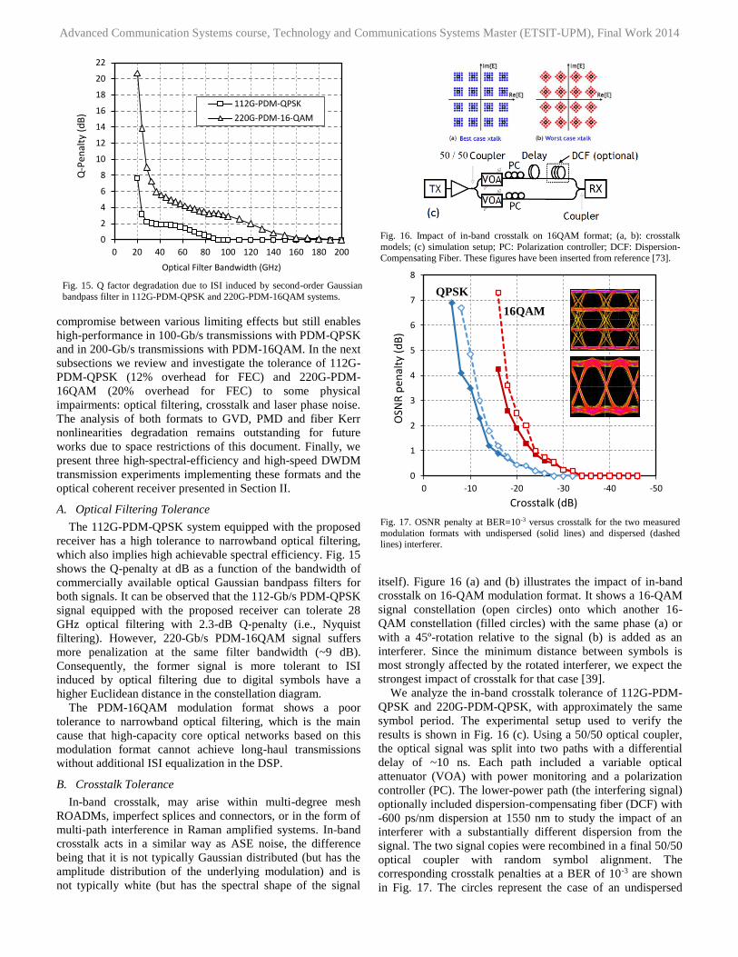
A. Optical Filtering Tolerance
The 112G-PDM-QPSK system equipped with the proposed
receiver has a high tolerance to narrowband optical filtering,
which also implies high achievable spectral efficiency. Fig. 15
shows the Q-penalty at dB as a function of the bandwidth of
commercially available optical Gaussian bandpass filters for
both signals. It can be observed that the 112-Gb/s PDM-QPSK
signal equipped with the proposed receiver can tolerate 28
GHz optical filtering with 2.3-dB Q-penalty (i.e., Nyquist
filtering). However, 220-Gb/s PDM-16QAM signal suffers
more penalization at the same filter bandwidth (~9 dB).
Consequently, the former signal is more tolerant to ISI
induced by optical filtering due to digital symbols have a
higher Euclidean distance in the constellation diagram.
The PDM-16QAM modulation format shows a poor
tolerance to narrowband optical filtering, which is the main
cause that high-capacity core optical networks based on this
modulation format cannot achieve long-haul transmissions
without additional ISI equalization in the DSP.
B. Crosstalk Tolerance
In-band crosstalk, may arise within multi-degree mesh
ROADMs, imperfect splices and connectors, or in the form of
multi-path interference in Raman amplified systems. In-band
crosstalk acts in a similar way as ASE noise, the difference
being that it is not typically Gaussian distributed (but has the
amplitude distribution of the underlying modulation) and is
not typically white (but has the spectral shape of the signal
itself). Figure 16 (a) and (b) illustrates the impact of in-band
crosstalk on 16-QAM modulation format. It shows a 16-QAM
signal constellation (open circles) onto which another 16-
QAM constellation (filled circles) with the same phase (a) or
with a 45º-rotation relative to the signal (b) is added as an
interferer. Since the minimum distance between symbols is
most strongly affected by the rotated interferer, we expect the
strongest impact of crosstalk for that case [39].
We analyze the in-band crosstalk tolerance of 112G-PDM-
QPSK and 220G-PDM-QPSK, with approximately the same
symbol period. The experimental setup used to verify the
results is shown in Fig. 16 (c). Using a 50/50 optical coupler,
the optical signal was split into two paths with a differential
delay of ~10 ns. Each path included a variable optical
attenuator (VOA) with power monitoring and a polarization
controller (PC). The lower-power path (the interfering signal)
optionally included dispersion-compensating fiber (DCF) with
-600 ps/nm dispersion at 1550 nm to study the impact of an
interferer with a substantially different dispersion from the
signal. The two signal copies were recombined in a final 50/50
optical coupler with random symbol alignment. The
corresponding crosstalk penalties at a BER of 10-3 are shown
in Fig. 17. The circles represent the case of an undispersed
Fig. 15. Q factor degradation due to ISI induced by second-order Gaussian
bandpass filter in 112G-PDM-QPSK and 220G-PDM-16QAM systems.
0
2
4
6
8
10
12
14
16
18
20
22
0 20 40 60 80 100 120 140 160 180 200
Q-P
enal
ty (
dB
)
Optical Filter Bandwidth (GHz)
112G-PDM-QPSK
220G-PDM-16-QAM
Fig. 16. Impact of in-band crosstalk on 16QAM format; (a, b): crosstalk
models; (c) simulation setup; PC: Polarization controller; DCF: Dispersion-
Compensating Fiber. These figures have been inserted from reference [73].
Fig. 17. OSNR penalty at BER=10-3 versus crosstalk for the two measured
modulation formats with undispersed (solid lines) and dispersed (dashed lines) interferer.
0
1
2
3
4
5
6
7
8
-50-40-30-20-100
OSN
R p
enal
ty (
dB
)
Crosstalk (dB)
QPSK
16QAM
Advanced Communication Systems course, Technology and Communications Systems Master (ETSIT-UPM), Final Work 2014
interferer (with a random phase relative to the signal), while
the squares are for the 600-ps/nm dispersed interferer. As
expected, introducing dispersion onto the interferer increases
crosstalk penalties due to the larger peak-to-average power
(PAPR) of the interfering signal, resulting in more severe
crosstalk-induced reductions of the minimum symbol distance
compared to a well-confined, undispersed interfering
constellation. Hence, the expansion of the symbols into sizable
clouds due to ISI leaves less room for further degradations by
crosstalk. For a 1-dB crosstalk penalty, our simulations allow
for average crosstalk levels of about –15 dB and –24 dB for
112G-PDM-QPSK and 220G-PDM-16-QAM, respectively.
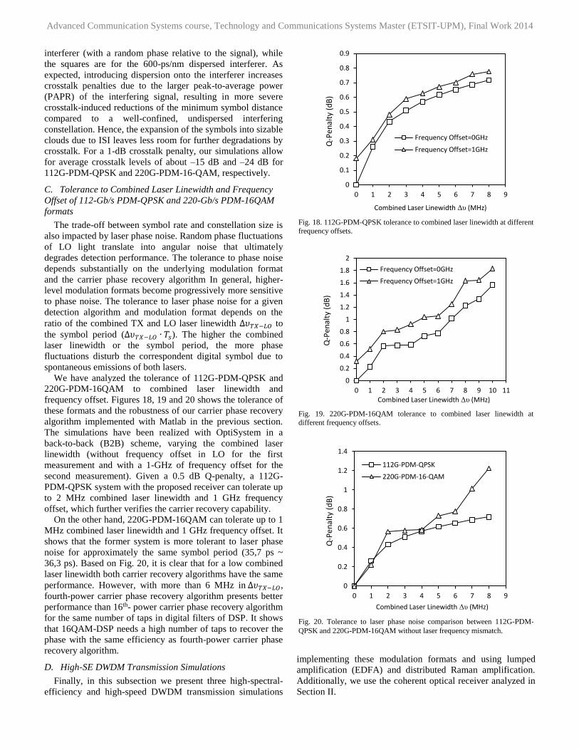
C. Tolerance to Combined Laser Linewidth and Frequency
Offset of 112-Gb/s PDM-QPSK and 220-Gb/s PDM-16QAM
formats
The trade-off between symbol rate and constellation size is
also impacted by laser phase noise. Random phase fluctuations
of LO light translate into angular noise that ultimately
degrades detection performance. The tolerance to phase noise
depends substantially on the underlying modulation format
and the carrier phase recovery algorithm In general, higher-
level modulation formats become progressively more sensitive
to phase noise. The tolerance to laser phase noise for a given
detection algorithm and modulation format depends on the
ratio of the combined TX and LO laser linewidth ∆𝜐𝑇𝑋−𝐿𝑂 to
the symbol period (∆𝜐𝑇𝑋−𝐿𝑂 ∙ 𝑇𝑠). The higher the combined
laser linewidth or the symbol period, the more phase
fluctuations disturb the correspondent digital symbol due to
spontaneous emissions of both lasers.
We have analyzed the tolerance of 112G-PDM-QPSK and
220G-PDM-16QAM to combined laser linewidth and
frequency offset. Figures 18, 19 and 20 shows the tolerance of
these formats and the robustness of our carrier phase recovery
algorithm implemented with Matlab in the previous section.
The simulations have been realized with OptiSystem in a
back-to-back (B2B) scheme, varying the combined laser
linewidth (without frequency offset in LO for the first
measurement and with a 1-GHz of frequency offset for the
second measurement). Given a 0.5 dB Q-penalty, a 112G-
PDM-QPSK system with the proposed receiver can tolerate up
to 2 MHz combined laser linewidth and 1 GHz frequency
offset, which further verifies the carrier recovery capability.
On the other hand, 220G-PDM-16QAM can tolerate up to 1
MHz combined laser linewidth and 1 GHz frequency offset. It
shows that the former system is more tolerant to laser phase
noise for approximately the same symbol period (35,7 ps ~
36,3 ps). Based on Fig. 20, it is clear that for a low combined
laser linewidth both carrier recovery algorithms have the same
performance. However, with more than 6 MHz in ∆𝜐𝑇𝑋−𝐿𝑂,
fourth-power carrier phase recovery algorithm presents better
performance than 16th- power carrier phase recovery algorithm
for the same number of taps in digital filters of DSP. It shows
that 16QAM-DSP needs a high number of taps to recover the
phase with the same efficiency as fourth-power carrier phase
recovery algorithm.
D. High-SE DWDM Transmission Simulations
Finally, in this subsection we present three high-spectral-
efficiency and high-speed DWDM transmission simulations
implementing these modulation formats and using lumped
amplification (EDFA) and distributed Raman amplification.
Additionally, we use the coherent optical receiver analyzed in
Section II.
Fig. 18. 112G-PDM-QPSK tolerance to combined laser linewidth at different
frequency offsets.
Fig. 19. 220G-PDM-16QAM tolerance to combined laser linewidth at
different frequency offsets.
Fig. 20. Tolerance to laser phase noise comparison between 112G-PDM-
QPSK and 220G-PDM-16QAM without laser frequency mismatch.
0
0.1
0.2
0.3
0.4
0.5
0.6
0.7
0.8
0.9
0 1 2 3 4 5 6 7 8 9
Q-P
enal
ty (
dB
)
Combined Laser Linewidth Δυ (MHz)
Frequency Offset=0GHz
Frequency Offset=1GHz
0
0.2
0.4
0.6
0.8
1
1.2
1.4
1.6
1.8
2
0 1 2 3 4 5 6 7 8 9 10 11
Q-P
enal
ty (
dB
)
Combined Laser Linewidth Δυ (MHz)
Frequency Offset=0GHz
Frequency Offset=1GHz
0
0.2
0.4
0.6
0.8
1
1.2
1.4
0 1 2 3 4 5 6 7 8 9
Q-P
enal
ty (
dB
)
Combined Laser Linewidth Δυ (MHz)
112G-PDM-QPSK
220G-PDM-16-QAM
Advanced Communication Systems course, Technology and Communications Systems Master (ETSIT-UPM), Final Work 2014
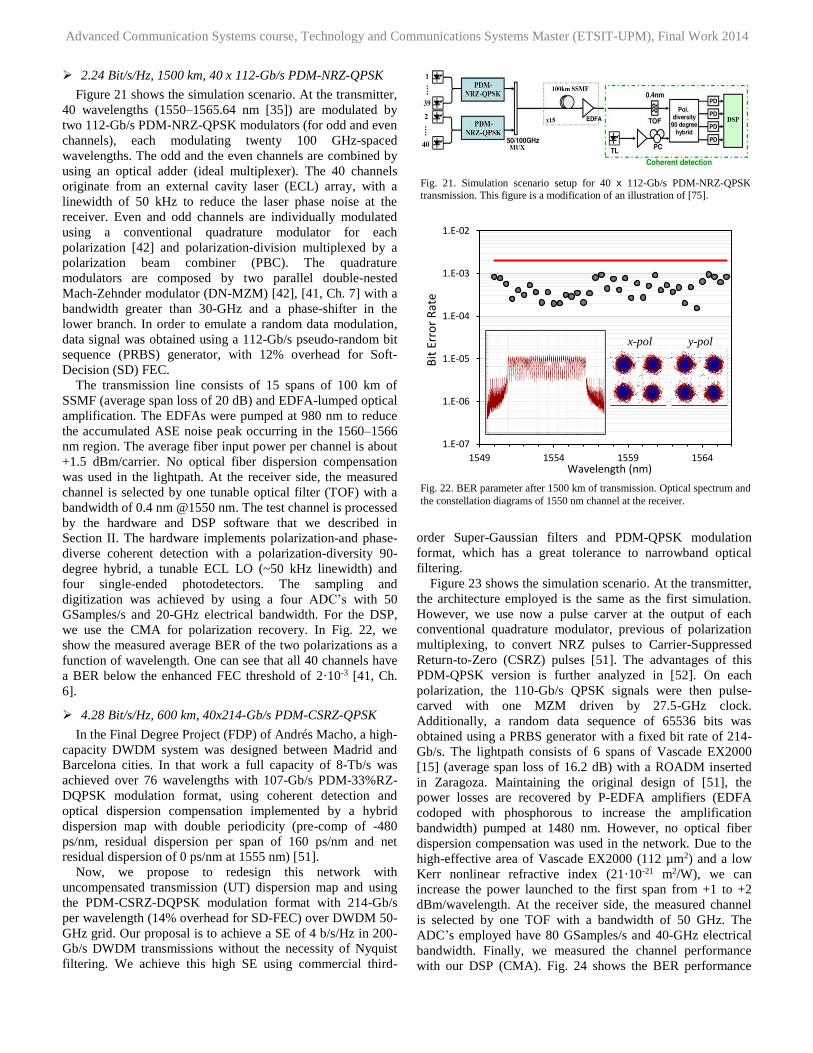
2.24 Bit/s/Hz, 1500 km, 40 x 112-Gb/s PDM-NRZ-QPSK
Figure 21 shows the simulation scenario. At the transmitter,
40 wavelengths (1550–1565.64 nm [35]) are modulated by
two 112-Gb/s PDM-NRZ-QPSK modulators (for odd and even
channels), each modulating twenty 100 GHz-spaced
wavelengths. The odd and the even channels are combined by
using an optical adder (ideal multiplexer). The 40 channels
originate from an external cavity laser (ECL) array, with a
linewidth of 50 kHz to reduce the laser phase noise at the
receiver. Even and odd channels are individually modulated
using a conventional quadrature modulator for each
polarization [42] and polarization-division multiplexed by a
polarization beam combiner (PBC). The quadrature
modulators are composed by two parallel double-nested
Mach-Zehnder modulator (DN-MZM) [42], [41, Ch. 7] with a
bandwidth greater than 30-GHz and a phase-shifter in the
lower branch. In order to emulate a random data modulation,
data signal was obtained using a 112-Gb/s pseudo-random bit
sequence (PRBS) generator, with 12% overhead for Soft-
Decision (SD) FEC.
The transmission line consists of 15 spans of 100 km of
SSMF (average span loss of 20 dB) and EDFA-lumped optical
amplification. The EDFAs were pumped at 980 nm to reduce
the accumulated ASE noise peak occurring in the 1560–1566
nm region. The average fiber input power per channel is about
+1.5 dBm/carrier. No optical fiber dispersion compensation
was used in the lightpath. At the receiver side, the measured
channel is selected by one tunable optical filter (TOF) with a
bandwidth of 0.4 nm @1550 nm. The test channel is processed
by the hardware and DSP software that we described in
Section II. The hardware implements polarization-and phase-
diverse coherent detection with a polarization-diversity 90-
degree hybrid, a tunable ECL LO (~50 kHz linewidth) and
four single-ended photodetectors. The sampling and
digitization was achieved by using a four ADC’s with 50
GSamples/s and 20-GHz electrical bandwidth. For the DSP,
we use the CMA for polarization recovery. In Fig. 22, we
show the measured average BER of the two polarizations as a
function of wavelength. One can see that all 40 channels have
a BER below the enhanced FEC threshold of 2·10-3 [41, Ch.
6].
4.28 Bit/s/Hz, 600 km, 40x214-Gb/s PDM-CSRZ-QPSK
In the Final Degree Project (FDP) of Andrés Macho, a high-
capacity DWDM system was designed between Madrid and
Barcelona cities. In that work a full capacity of 8-Tb/s was
achieved over 76 wavelengths with 107-Gb/s PDM-33%RZ-
DQPSK modulation format, using coherent detection and
optical dispersion compensation implemented by a hybrid
dispersion map with double periodicity (pre-comp of -480
ps/nm, residual dispersion per span of 160 ps/nm and net
residual dispersion of 0 ps/nm at 1555 nm) [51].
Now, we propose to redesign this network with
uncompensated transmission (UT) dispersion map and using
the PDM-CSRZ-DQPSK modulation format with 214-Gb/s
per wavelength (14% overhead for SD-FEC) over DWDM 50-
GHz grid. Our proposal is to achieve a SE of 4 b/s/Hz in 200-
Gb/s DWDM transmissions without the necessity of Nyquist
filtering. We achieve this high SE using commercial third-
order Super-Gaussian filters and PDM-QPSK modulation
format, which has a great tolerance to narrowband optical
filtering.
Figure 23 shows the simulation scenario. At the transmitter,
the architecture employed is the same as the first simulation.
However, we use now a pulse carver at the output of each
conventional quadrature modulator, previous of polarization
multiplexing, to convert NRZ pulses to Carrier-Suppressed
Return-to-Zero (CSRZ) pulses [51]. The advantages of this
PDM-QPSK version is further analyzed in [52]. On each
polarization, the 110-Gb/s QPSK signals were then pulse-
carved with one MZM driven by 27.5-GHz clock.
Additionally, a random data sequence of 65536 bits was
obtained using a PRBS generator with a fixed bit rate of 214-
Gb/s. The lightpath consists of 6 spans of Vascade EX2000
[15] (average span loss of 16.2 dB) with a ROADM inserted
in Zaragoza. Maintaining the original design of [51], the
power losses are recovered by P-EDFA amplifiers (EDFA
codoped with phosphorous to increase the amplification
bandwidth) pumped at 1480 nm. However, no optical fiber
dispersion compensation was used in the network. Due to the
high-effective area of Vascade EX2000 (112 µm2) and a low
Kerr nonlinear refractive index (21·10-21 m2/W), we can
increase the power launched to the first span from +1 to +2
dBm/wavelength. At the receiver side, the measured channel
is selected by one TOF with a bandwidth of 50 GHz. The
ADC’s employed have 80 GSamples/s and 40-GHz electrical
bandwidth. Finally, we measured the channel performance
with our DSP (CMA). Fig. 24 shows the BER performance
Fig. 21. Simulation scenario setup for 40 x 112-Gb/s PDM-NRZ-QPSK
transmission. This figure is a modification of an illustration of [75].
Fig. 22. BER parameter after 1500 km of transmission. Optical spectrum and
the constellation diagrams of 1550 nm channel at the receiver.
1.E-07
1.E-06
1.E-05
1.E-04
1.E-03
1.E-02
1549 1554 1559 1564
Bit
Err
or
Rat
e
Wavelength (nm)
x-pol y-pol
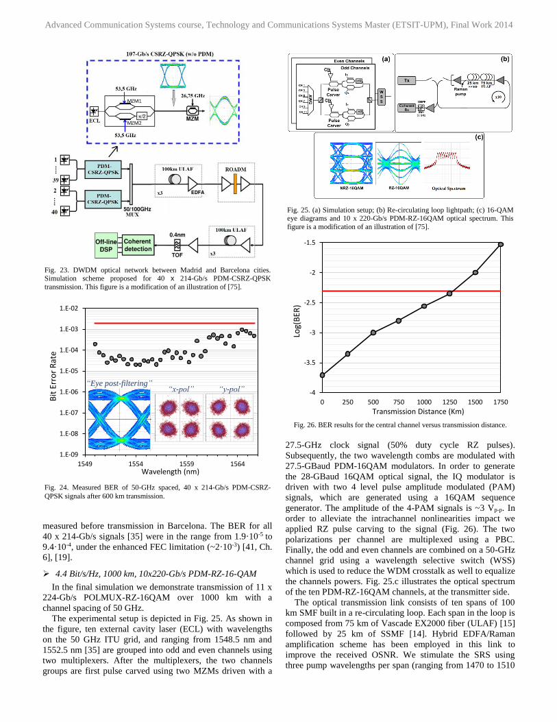
Advanced Communication Systems course, Technology and Communications Systems Master (ETSIT-UPM), Final Work 2014
measured before transmission in Barcelona. The BER for all
40 x 214-Gb/s signals [35] were in the range from 1.9·10-5 to
9.4·10-4, under the enhanced FEC limitation (~2·10-3) [41, Ch.
6], [19].
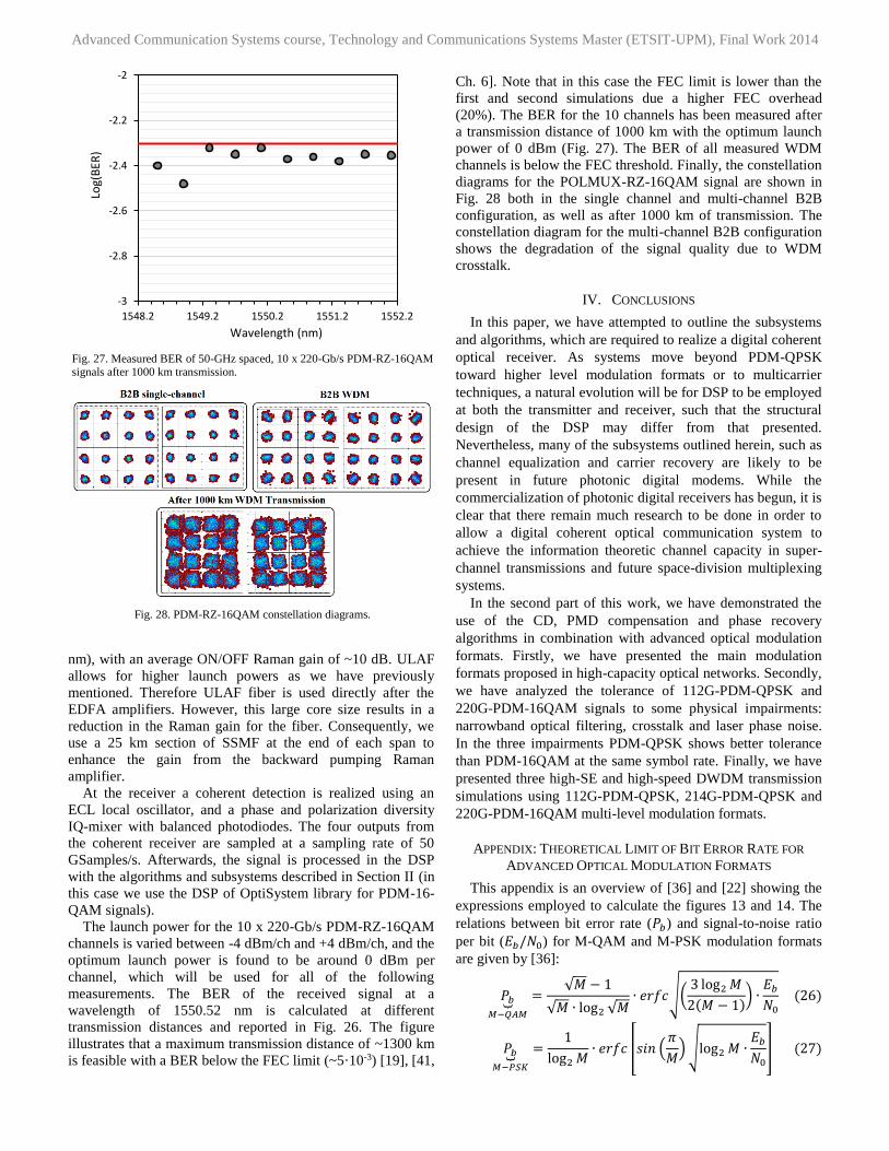
4.4 Bit/s/Hz, 1000 km, 10x220-Gb/s PDM-RZ-16-QAM
In the final simulation we demonstrate transmission of 11 x
224-Gb/s POLMUX-RZ-16QAM over 1000 km with a
channel spacing of 50 GHz.
The experimental setup is depicted in Fig. 25. As shown in
the figure, ten external cavity laser (ECL) with wavelengths
on the 50 GHz ITU grid, and ranging from 1548.5 nm and
1552.5 nm [35] are grouped into odd and even channels using
two multiplexers. After the multiplexers, the two channels
groups are first pulse carved using two MZMs driven with a
27.5-GHz clock signal (50% duty cycle RZ pulses).
Subsequently, the two wavelength combs are modulated with
27.5-GBaud PDM-16QAM modulators. In order to generate
the 28-GBaud 16QAM optical signal, the IQ modulator is
driven with two 4 level pulse amplitude modulated (PAM)
signals, which are generated using a 16QAM sequence
generator. The amplitude of the 4-PAM signals is ~3 Vp-p. In
order to alleviate the intrachannel nonlinearities impact we
applied RZ pulse carving to the signal (Fig. 26). The two
polarizations per channel are multiplexed using a PBC.
Finally, the odd and even channels are combined on a 50-GHz
channel grid using a wavelength selective switch (WSS)
which is used to reduce the WDM crosstalk as well to equalize
the channels powers. Fig. 25.c illustrates the optical spectrum
of the ten PDM-RZ-16QAM channels, at the transmitter side.
The optical transmission link consists of ten spans of 100
km SMF built in a re-circulating loop. Each span in the loop is
composed from 75 km of Vascade EX2000 fiber (ULAF) [15]
followed by 25 km of SSMF [14]. Hybrid EDFA/Raman
amplification scheme has been employed in this link to
improve the received OSNR. We stimulate the SRS using
three pump wavelengths per span (ranging from 1470 to 1510
Fig. 23. DWDM optical network between Madrid and Barcelona cities. Simulation scheme proposed for 40 x 214-Gb/s PDM-CSRZ-QPSK
transmission. This figure is a modification of an illustration of [75].
Fig. 24. Measured BER of 50-GHz spaced, 40 x 214-Gb/s PDM-CSRZ-
QPSK signals after 600 km transmission.
1.E-09
1.E-08
1.E-07
1.E-06
1.E-05
1.E-04
1.E-03
1.E-02
1549 1554 1559 1564
Bit
Err
or
Rat
e
Wavelength (nm)
Fig. 25. (a) Simulation setup; (b) Re-circulating loop lightpath; (c) 16-QAM eye diagrams and 10 x 220-Gb/s PDM-RZ-16QAM optical spectrum. This
figure is a modification of an illustration of [75].
Fig. 26. BER results for the central channel versus transmission distance.
-4
-3.5
-3
-2.5
-2
-1.5
0 250 500 750 1000 1250 1500 1750
Log(
BER
)
Transmission Distance (Km)
“Eye post-filtering”
“x-pol” “y-pol”
Advanced Communication Systems course, Technology and Communications Systems Master (ETSIT-UPM), Final Work 2014
nm), with an average ON/OFF Raman gain of ~10 dB. ULAF
allows for higher launch powers as we have previously
mentioned. Therefore ULAF fiber is used directly after the
EDFA amplifiers. However, this large core size results in a
reduction in the Raman gain for the fiber. Consequently, we
use a 25 km section of SSMF at the end of each span to
enhance the gain from the backward pumping Raman
amplifier.
At the receiver a coherent detection is realized using an
ECL local oscillator, and a phase and polarization diversity
IQ-mixer with balanced photodiodes. The four outputs from
the coherent receiver are sampled at a sampling rate of 50
GSamples/s. Afterwards, the signal is processed in the DSP
with the algorithms and subsystems described in Section II (in
this case we use the DSP of OptiSystem library for PDM-16-
QAM signals).
The launch power for the 10 x 220-Gb/s PDM-RZ-16QAM
channels is varied between -4 dBm/ch and +4 dBm/ch, and the
optimum launch power is found to be around 0 dBm per
channel, which will be used for all of the following
measurements. The BER of the received signal at a
wavelength of 1550.52 nm is calculated at different
transmission distances and reported in Fig. 26. The figure
illustrates that a maximum transmission distance of ~1300 km
is feasible with a BER below the FEC limit (~5·10-3) [19], [41,
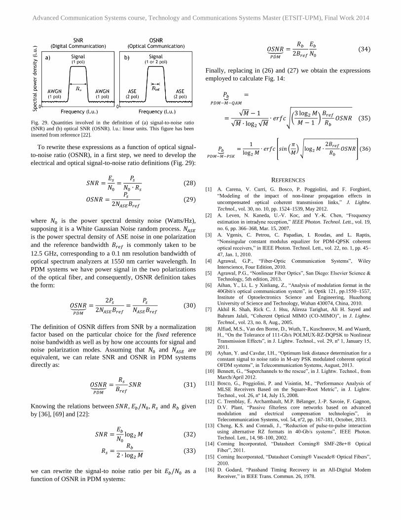
Ch. 6]. Note that in this case the FEC limit is lower than the
first and second simulations due a higher FEC overhead
(20%). The BER for the 10 channels has been measured after
a transmission distance of 1000 km with the optimum launch
power of 0 dBm (Fig. 27). The BER of all measured WDM
channels is below the FEC threshold. Finally, the constellation
diagrams for the POLMUX-RZ-16QAM signal are shown in
Fig. 28 both in the single channel and multi-channel B2B
configuration, as well as after 1000 km of transmission. The
constellation diagram for the multi-channel B2B configuration
shows the degradation of the signal quality due to WDM
crosstalk.
IV. CONCLUSIONS
In this paper, we have attempted to outline the subsystems
and algorithms, which are required to realize a digital coherent
optical receiver. As systems move beyond PDM-QPSK
toward higher level modulation formats or to multicarrier
techniques, a natural evolution will be for DSP to be employed
at both the transmitter and receiver, such that the structural
design of the DSP may differ from that presented.
Nevertheless, many of the subsystems outlined herein, such as
channel equalization and carrier recovery are likely to be
present in future photonic digital modems. While the
commercialization of photonic digital receivers has begun, it is
clear that there remain much research to be done in order to
allow a digital coherent optical communication system to
achieve the information theoretic channel capacity in super-
channel transmissions and future space-division multiplexing
systems.
In the second part of this work, we have demonstrated the
use of the CD, PMD compensation and phase recovery
algorithms in combination with advanced optical modulation
formats. Firstly, we have presented the main modulation
formats proposed in high-capacity optical networks. Secondly,
we have analyzed the tolerance of 112G-PDM-QPSK and
220G-PDM-16QAM signals to some physical impairments:
narrowband optical filtering, crosstalk and laser phase noise.
In the three impairments PDM-QPSK shows better tolerance
than PDM-16QAM at the same symbol rate. Finally, we have
presented three high-SE and high-speed DWDM transmission
simulations using 112G-PDM-QPSK, 214G-PDM-QPSK and
220G-PDM-16QAM multi-level modulation formats.
APPENDIX: THEORETICAL LIMIT OF BIT ERROR RATE FOR
ADVANCED OPTICAL MODULATION FORMATS
This appendix is an overview of [36] and [22] showing the
expressions employed to calculate the figures 13 and 14. The
relations between bit error rate (𝑃𝑏) and signal-to-noise ratio
per bit (𝐸𝑏/𝑁0) for M-QAM and M-PSK modulation formats
are given by [36]:
𝑃𝑏⏟𝑀−𝑄𝐴𝑀
=√𝑀 − 1
√𝑀 ∙ log2 √𝑀∙ 𝑒𝑟𝑓𝑐√(
3 log2𝑀
2(𝑀 − 1)) ∙𝐸𝑏𝑁0 (26)
𝑃𝑏⏟𝑀−𝑃𝑆𝐾
=1
log2𝑀∙ 𝑒𝑟𝑓𝑐 [𝑠𝑖𝑛 (
𝜋
𝑀)√log2𝑀 ∙
𝐸𝑏𝑁0] (27)
Fig. 27. Measured BER of 50-GHz spaced, 10 x 220-Gb/s PDM-RZ-16QAM signals after 1000 km transmission.
Fig. 28. PDM-RZ-16QAM constellation diagrams.
-3
-2.8
-2.6
-2.4
-2.2
-2
1548.2 1549.2 1550.2 1551.2 1552.2
Log(
BER
)
Wavelength (nm)
Advanced Communication Systems course, Technology and Communications Systems Master (ETSIT-UPM), Final Work 2014
To rewrite these expressions as a function of optical signal-
to-noise ratio (OSNR), in a first step, we need to develop the
electrical and optical signal-to-noise ratio definitions (Fig. 29):
𝑆𝑁𝑅 =𝐸𝑠𝑁0=
𝑃𝑠𝑁0 ∙ 𝑅𝑠
(28)
𝑂𝑆𝑁𝑅 =𝑃𝑠
2𝑁𝐴𝑆𝐸𝐵𝑟𝑒𝑓 (29)
where 𝑁0 is the power spectral density noise (Watts/Hz),
supposing it is a White Gaussian Noise random process. 𝑁𝐴𝑆𝐸
is the power spectral density of ASE noise in one polarization
and the reference bandwidth 𝐵𝑟𝑒𝑓 is commonly taken to be
12.5 GHz, corresponding to a 0.1 nm resolution bandwidth of
optical spectrum analyzers at 1550 nm carrier wavelength. In
PDM systems we have power signal in the two polarizations
of the optical fiber, and consequently, OSNR definition takes
the form:
𝑂𝑆𝑁𝑅⏟ 𝑃𝐷𝑀
=2𝑃𝑠
2𝑁𝐴𝑆𝐸𝐵𝑟𝑒𝑓=
𝑃𝑠𝑁𝐴𝑆𝐸𝐵𝑟𝑒𝑓
(30)
The definition of OSNR differs from SNR by a normalization
factor based on the particular choice for the fixed reference
noise bandwidth as well as by how one accounts for signal and
noise polarization modes. Assuming that 𝑁0 and 𝑁𝐴𝑆𝐸 are
equivalent, we can relate SNR and OSNR in PDM systems
directly as:
𝑂𝑆𝑁𝑅⏟ 𝑃𝐷𝑀
=𝑅𝑠𝐵𝑟𝑒𝑓
𝑆𝑁𝑅 (31)
Knowing the relations between 𝑆𝑁𝑅, 𝐸𝑏/𝑁0, 𝑅𝑠 and 𝑅𝑏 given
by [36], [69] and [22]:
𝑆𝑁𝑅 =𝐸𝑏𝑁0log2𝑀 (32)
𝑅𝑠 =𝑅𝑏
2 ∙ log2𝑀 (33)
we can rewrite the signal-to noise ratio per bit 𝐸𝑏/𝑁0 as a
function of OSNR in PDM systems:
𝑂𝑆𝑁𝑅⏟ 𝑃𝐷𝑀
=𝑅𝑏2𝐵𝑟𝑒𝑓
𝐸𝑏𝑁0 (34)
Finally, replacing in (26) and (27) we obtain the expressions
employed to calculate Fig. 14:
𝑃𝑏⏟𝑃𝐷𝑀−𝑀−𝑄𝐴𝑀
=
=√𝑀 − 1
√𝑀 ∙ log2 √𝑀∙ 𝑒𝑟𝑓𝑐√(
3 log2𝑀
𝑀 − 1)𝐵𝑟𝑒𝑓
𝑅𝑏𝑂𝑆𝑁𝑅 (35)
𝑃𝑏⏟𝑃𝐷𝑀−𝑀−𝑃𝑆𝐾
=1
log2𝑀∙ 𝑒𝑟𝑓𝑐 [𝑠𝑖𝑛 (
𝜋
𝑀)√log2𝑀 ∙
2𝐵𝑟𝑒𝑓
𝑅𝑏𝑂𝑆𝑁𝑅] (36)
REFERENCES
[1] A. Carena, V. Curri, G. Bosco, P. Poggiolini, and F. Forghieri,
“Modeling of the impact of non-linear propagation effects in
uncompensated optical coherent transmission links,” J. Lightw.
Technol., vol. 30, no. 10, pp. 1524–1539, May 2012.
[2] A. Leven, N. Kaneda, U.-V. Koc, and Y.-K. Chen, “Frequency
estimation in intradyne reception,” IEEE Photon. Technol. Lett., vol. 19,
no. 6, pp. 366–368, Mar. 15, 2007.
[3] A. Vgenis, C. Petrou, C. Papadias, I. Roudas, and L. Raptis,
“Nonsingular constant modulus equalizer for PDM-QPSK coherent
optical receivers,” in IEEE Photon. Technol. Lett., vol. 22, no. 1, pp. 45–
47, Jan. 1, 2010.
[4] Agrawal, G.P., “Fiber-Optic Communication Systems”, Wiley
Interscience, Four Edition, 2010.
[5] Agrawal, P.G., “Nonlinear Fiber Optics”, San Diego: Elsevier Science & Technology, 5th edition, 2013.
[6] Aihan, Y., Li, L. y Xinliang, Z., “Analysis of modulation format in the
40Gbit/s optical communication system”, in Optik 121, pp.1550–1557, Institute of Optoelectronics Science and Engineering, Huazhong
University of Science and Technology, Wuhan 430074, China, 2010.
[7] Akhil R. Shah, Rick C. J. Hsu, Alireza Tarighat, Ali H. Sayed and
Bahram Jalali, “Coherent Optical MIMO (CO-MIMO)”, in J. Lightw.
Technol., vol. 23, no. 8, Aug., 2005.
[8] Alfiad, M.S., Van den Borne, D., Wuth, T., Kuschnerov, M. and Waardt, H., “On the Tolerance of 111-Gb/s POLMUX-RZ-DQPSK to Nonlinear
Transmission Effects”, in J. Lightw. Technol., vol. 29, nº 1, January 15,
2011. [9] Ayhan, Y. and Cavdar, I.H., “Optimum link distance determination for a
constant signal to noise ratio in M-ary PSK modulated coherent optical
OFDM systems”, in Telecommunication Systems, August, 2013. [10] Bennett, G., “Superchannels to the rescue”, in J. Lightw. Technol., from
March/April 2012.
[11] Bosco, G., Poggiolini, P. and Visintin, M., “Performance Analysis of MLSE Receivers Based on the Square-Root Metric”, in J. Lightw.
Technol., vol. 26, nº 14, July 15, 2008.
[12] C. Tremblay, É. Archambault, M.P. Bélanger, J.-P. Savoie, F. Gagnon, D.V. Plant, “Passive filterless core networks based on advanced
modulation and electrical compensation technologies”, in
Telecommunication Systems, vol. 54, nº2, pp. 167-181, October, 2013. [13] Cheng, K.S. and Conradi, J., “Reduction of pulse-to-pulse interaction
using alternative RZ formats in 40-Gb/s systems”, IEEE Photon.
Technol. Lett., 14, 98–100, 2002. [14] Corning Incorporated, “Datasheet Corning® SMF-28e+® Optical
Fiber”, 2011.
[15] Corning Incorporated, “Datasheet Corning® Vascade® Optical Fibers”,
2010.
[16] D. Godard, “Passband Timing Recovery in an All-Digital Modem
Receiver,” in IEEE Trans. Commun. 26, 1978.
Fig. 29. Quantities involved in the definition of (a) signal-to-noise ratio (SNR) and (b) optical SNR (OSNR). l.u.: linear units. This figure has been
inserted from reference [22].
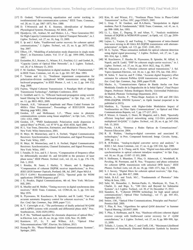
Advanced Communication Systems course, Technology and Communications Systems Master (ETSIT-UPM), Final Work 2014
[17] D. Godard, “Self-recovering equalization and carrier tracking in
twodimensional data communication systems,” IEEE Trans. Commun.,
vol. 28, no. 11, pp. 1867–1875, Nov. 1980.
[18] D. T.Westwick and R. E. Kearney, Identification of Nonlinear
Physiological Systems. Piscataway, NJ: IEEE, 2003.
[19] Djordjevic, I.B., Arabaci, M. and Minkov, L.L., “Next Generation FEC
for High-Capacity Communication in Optical Transport Networks”, in J.
Lightw. Technol., vol. 27, no. 16, Aug. 15, 2009.
[20] E. Ip and J. Kahn, “Feedforward carrier recovery for coherent optical
communications,” J. Lightw. Technol., vol. 25, no. 9, pp. 2675–2692,
Sep. 2007.
[21] Elbers, J.P., “Modelling of polarization mode dispersion in single mode
fibers”, in Electronics Letters. Vol. 33 nº 22, pp. 1894-1895, October, 1997.
[22] Essiambre, R.J., Kramer, G., Winzer, P.J., Foschini, G.J. and Goebel, B.,
“Capacity Limits of Optical Fiber Networks”, in J. Lightw. Technol.,
vol. 28, nº 4, February 15, 2010.
[23] F. M. Gardner, “Interpolation in digital modems. Part I: Fundamentals,”
in IEEE Trans. Commun., vol. 41, no. 3, pp. 501–507, Mar. 1993.
[24] F. Yaman and G. Li, “Nonlinear impairment compensation for
polarization-division multiplexed WDM transmission using digital
backward propagation,” in IEEE Photon. J., vol. 1, no. 2, pp. 144–152,
Aug. 2009.
[25] Fujitsu, “Digital Coherent Transmission: A Paradigm Shift of Optical
Transmission Technology”, SubOptic Conference, 2010.
[26] G. Goldfarb and G. Li, “Efficient backward-propagation using wavelet
based filtering for fiber backward-propagation,” in Opt. Exp., vol. 17,
no. 11, pp. 8815–8821, 2009.
[27] Gnauck, A.H., “Advanced Amplitude and Phase Coded Formats for
40Gb/s Fiber Transmission”, Proceedings of IEEE/LEOS Annual
Meeting, page WR1, 2004. [28] Gordon, J.P. and Mollenauer, L.F., “Phase noise in photonic
communications systems using linear amplifiers”, in Opt. Lett., 15(23),
1351–1353, 1990. [29] Gordon, J.P., “PMD fundamentals: Polarization mode dispersion in
optical fibers” in PNAS., vol. 97 Nº 9, pp. 4541-4550, April 2000. [30] H. L. Van Trees, Detection, Estimation, and Modulation Theory, Part I.
New York: Wiley Interscience, 2001.
[31] H. Meyr, M. Moeneclaey, and S. A. Fechtel, “Digital Communication
Receivers: Synchronization, Channel Estimation, and Signal Processing.
New York: Wiley, 1997.
[32] H. Meyr, M. Moeneclaey, and S. A. Fechtel, Digital Communication
Receivers: Synchronization, Channel Estimation, and Signal Processing.
New York: Wiley, 1997.
[33] I. Fatadin, D. Ives, and S. J. Savory, “Compensation of frequency offset
for differentially encoded 16- and 64-QAM in the presence of laser
phase noise,” IEEE Photon. Technol. Lett., vol. 22, no. 3, pp. 176–178,
Feb. 1, 2010.
[34] I. Roudas, M. Sauer, J. Hurley, Y. Mauro, and S. Raghavan,
“Compensation of coherent DQPSK receiver imperfections,” in Proc.
IEEE LEOS Summer Topicals, Portland, OR, Jul. 2007, Paper MA3.4.
[35] ITU-T G.694.1 Recommendation (2012), “Spectral grids for WDM
applications: DWDM frequency grid”.
[36] J. G. Proakis, Digital Communications, 4th ed. New York: McGraw-
Hill, 2001.
[37] K. Mueller and M. Muller, “Timing recovery in digital synchronous data
receivers,” IEEE Trans. Commun., vol. COM-24, no. 5, pp. 516–531,
May 1976.
[38] K. Piyawanno, M. Kuschnerov, B. Spinnler, and B. Lankl, “Fast and
accurate automatic frequency control for coherent receivers,” in Proc.
Eur. Conf. Opt. Commun., Sep. 2009, paper 7.3.1.
[39] K. V. Cartwright et al., “The performance of dually polarized M-QAM
and L-QPRS systems with crosstalk and differential phase shift,” Proc.
Southeastcon., 1026-1029 (1991).
[40] K.-P. Ho, “Subband equaliser for chromatic dispersion of optical fibre,”
in Electron. Lett., vol. 45, no. 24, pp. 1224–1226, Nov. 19, 2009.
[41] Kaminow, I.P., Li, T. and Willner, A.E., “Optical Fiber
Telecommunications VIB”, Elsevier, Six Edition, 2013.
[42] Keang-Po Ho, “Phase-Modulated Optical Communications Systems”, Springer, 2005.
[43] Kim, H. and Winzer, P.J., “Nonlinear Phase Noise in Phase-Coded
Transmission”, in Proc. OFC, page OThO3, 2005.
[44] L. Erup, F. M. Gardner, and R.A.Harris, “Interpolation in digital
modems. Part II: Fundamentals,” IEEE Trans. Commun., vol. 41, no. 6,
pp. 998–1008, Jun. 1993.
[45] Li, L., Jijun, Z., Degong, D. and Aihan, Y., “Analysis modulation formats of DQPSK in WDM-PON system”, in Optik, vol. 123, pp. 2050-
2055, 2012. [46] Lujiao, L., Yaojun, Q. and Yuefeng, J., “Suppression of intra-channel
four-wave mixing in 40 Gbit/s RZ-DQPSK transmission with alternate-
polarization”, in Optik, vol. 122, pp. 2242– 2245, 2011. [47] M. G. Taylor, “Phase estimation methods for optical coherent detection
using digital signal processing,” J. Lightw. Technol., vol. 27, no. 7, pp.
901–914, Apr. 1, 2009.
[48] M. Kuschnerov, F. Hauske, K. Piyawanno, B. Spinnler, M. Alfiad, A.
Napoli, and B. Lankl, “DSP for coherent single-carrier receivers,” in J.
Lightw. Technol., vol. 27, no. 16, pp. 3614–3622, Aug. 15, 2009.
[49] M. Nakazawa et al., “Ultrafast coherent optical transmission,” J. Sel.
Topics Quantum Electron., vol. 18, no. 1, pp. 363–376, Jan.–Feb. 2012.
[50] M. Selmi, Y. Jaou¨en, and P. Ciblat, “Accurate digital frequency offset
estimator for coherent PolMux QAM transmission systems,” in Proc.
Eur. Conf. Opt. Commun., Sep. 2009, paper P3.08.
[51] Macho, A., “Comunicaciones Ópticas de Banda Ancha con Fase
Modulada: Estudio de la Degradación de la Señal Óptica”, Final Project
Degree, Professor: Paloma Rodríguez Horche, Universidad Politécnica
de Madrid, Photonic Technology Department, 2013.
[52] Macho, A., Horche, P., “Pulse-Shape Analysis in 100 and 200 Gb/s
PDM-(D)QPSK DWDM Systems”, in Optik Journal (expected to be
published in 2015).
[53] Matthias, S., “Systems with Higher-Order Modulation Impact of Nonlinearities on Fiber Optic Communications”, in Optical and Fiber
Communications Reports, vol. 7, pp. 177-217, 2011.
[54] P. Winzer, A. Gnauck, C. Doerr, M. Magarini, and L. Buhl, “Spectrally
efficient long-haul optical networking using 112-Gb/s polarization
multiplexed 16-QAM,” J. Lightw. Technol., vol. 28, no. 4, pp. 547–556,
Feb. 15, 2010.
[55] Pereda, J.A.M., “Sistemas y Redes Ópticas de Comunicaciones”.
Pearson Educacion. 2004.
[56] R. H. Walden, “Analog-to-digital converters and associated IC
technologies,” in Proc. Compound Semicond. Integr. Circuits. Symp.,
2008, pp. 1–2.
[57] R. H.Walden, “Analog-to-digital converter survey and analysis,” in
IEEE J. Sel. Areas Commun., vol. 17, no. 4, pp. 539–550, Apr. 1999.
[58] S. H. Chang, H. S. Chung, and K. Kim, “Digital non-data-aided symbol
synchronization in optical coherent intradyne reception,” in Opt. Exp.,
vol. 16, no. 19, pp. 15 097–15 103, 2008.
[59] S. Hoffmann, S. Bhandare, T. Pfau, O. Adamczyk, C. Wordehoff, R.
Peveling, M. Porrmann, and R. Noe, “Frequency and phase estimation
for coherent QPSK transmission with unlocked DFB lasers,” IEEE
Photon. Technol. Letts, vol. 20, no. 18, pp. 1569–1571, Sep. 15, 2008.
[60] S. J. Savory, “Digital filters for coherent optical receivers,” Opt. Exp.,
vol. 16, no. 2, pp. 804–817, 2008.
[61] Saleh, B.A.E. and Teich, M.C., “Fundamentals of Photonics” John
Wiley & Sons, 1991. [62] Salsi, M., Renaudier, J., Bertran-Pardo, O., Mardoyan, H., Tran, P.,
Charlet, G. and Bigo, S., “100 Gb/s and Beyond for Submarine
Systems”, in J. Lightw. Technol., vol. 30, nº 24, December 15, 2012. [63] Saunders, R., “Coherent DWDM technology for high speed optical
communications”, Optical Fiber Technology., vol 17, pp. 445–451,
September 2011. [64] Senior, J.M., “Optical Fiber Communications, Principles and Practice”.
Prentice Hall. 2009.
[65] T. Pfau, R. Noe, “Algorithms for optical QAM detection” in Summer
Topical Meeting, LEOSST 2009.
[66] T. Pfau, S. Hoffmann, and R. Noe, “Hardware-efficient coherent digital
receiver concept with feedforward carrier recovery for M -QAM
constellations,” in J. Lightw. Technol., vol. 27, no. 8, pp. 989–999, Apr.
15, 2009.
[67] Tellado, J., Louise, M., Hoo, C. and Cioffi, J.M., “Maximum-Likelihood Detection of Nonlinearly Distorted Multicarrier Symbols by Iterative

Advanced Communication Systems course, Technology and Communications Systems Master (ETSIT-UPM), Final Work 2014
Decoding”, in IEEE Transactions on Communications, vol. 51, no. 2,
February, 2003.
[68] Wang, J., Xie, C. and Pan, Z., “Generation of Spectrally Efficient
Nyquist-WDM QPSK Signals Using Digital FIR or FDE Filters at
Transmitter”, in J. Lightw. Technol., vol. 30, nº 23, December 1, 2012. [69] Winzer, P.J. and Essiambre, R.J., “Advanced optical modulation
formats”, Proc. IEEE, vol.94, nº 5, pp.952-985, May 2006.
[70] Winzer, P.J. and Essiambre, R.J., “Advanced optical modulation formats”, in Optical Fiber Telecommunications, 2008.
[71] Winzer, P.J. and Gnauck, A.H., “Optical Phase-Shift-Keyed
Transmision”, in J. Lightw. Technol., 23(1), 115–130, 2005. [72] Winzer, P.J., “High-Spectral-Efficiency Optical Modulation Formats”,
in J. Lightw. Technol., vol. 30, nº 24, December 15, 2012.
[73] Winzer, P.J. et al., “Penalties from In-Band Crosstalk for Advanced
Optical Modulation Formats”, in ECOC 2011, paper Tu.5.B.7.
[74] Yu, J., Dong, Z., Chien, H.-C., Jia, Z., Li, X., Huo, D., Gunkel, M.,
Wagner, P., Mayer, H. and Schippel, A., “Transmission of 200 G PDM-CSRZ-QPSK and PDM-16QAM with a SE of 4 b/s/Hz”, in J. Lightw.
Technol., vol. 31, nº 4, February 15, 2013.
[75] Zhou, X. and Yu, J., “Multi-Level, Multi-Dimensional Coding for High-
Speed and High-Spectral-Efficiency Optical Transmission”, in J.
Lightw. Technol., vol. 27, nº 16, August 15, 2009.
Andrés Macho received the
Telecommunication Engineering
degree (M.S.) from the ETSIT-
Universidad Politécnica de Madrid in
2013. Currently, he is working
towards his Ph.D. degree at
Nanophotonics Technology Center
Universidad Politécnica de Valencia
(Spain). His professional interest
includes high-capacity wavelength-
division multiplexed systems (WDM),
advanced optical modulation formats
and space-division multiplexing for
optical networks. He worked in 2013
at Telefonica R&D Corporation in the
Core Network Evolution group involved in some R&D European projects
(INSPACE, STRAUSS and DISCUS).