digital commons - liberty university research

Running head: HYPERBOLIC CONFORMAL TRANSFORMATIONS 1

Examples of Solving the Wave Equation in the Hyperbolic Plane

Cooper Ramsey

A Senior Thesis submitted in partial fulfillment

of the requirements for graduation

in the Honors Program

Liberty University

Spring 2018

HYPERBOLIC CONFORMAL TRANSFORMATIONS

2

Acceptance of Senior Honors Thesis

This Senior Honors Thesis is accepted in partial

fulfillment of the requirements for graduation from the

Honors Program of Liberty University.

______________________________

James Cook, Ph.D.

Thesis Chair

______________________________

Hector Medina, Ph.D.

Committee Member

______________________________

David Wang, Ph.D.

Committee Member

______________________________

David Schweitzer, Ph.D.

Assistant Honors Director

______________________________

Date


3

Abstract

The complex numbers have proven themselves immensely useful in physics,

mathematics, and engineering. One useful tool of the complex numbers is the method of

conformal mapping which is used to solve various problems in physics and engineering

that involved Laplace’s equation. Following the work done by Dr. James Cook, the

complex numbers are replaced with associative real algebras. This paper focuses on

another algebra, the hyperbolic numbers. A solution method like conformal mapping is

developed with solutions to the one-dimensional wave equation. Applications of this

solution method revolve around engineering and physics problems involving the

propagation of waves. To conclude, a series of examples and transformations are given to

demonstrate the solution method.

Keywords: hyperbolic, Fourier, associative real algebra, wave equation


4

Examples of Solving the Wave Equation in the Hyperbolic Plane

Introduction

Conformal mapping refers to local angle preserving transformation functions

called conformal maps. These maps turn out to be profoundly useful in physics when

looking at them in the complex number plane. Certain transformation functions in the

complex plane are solutions to Laplace's equation which is the equation governing the

temperature distribution in two-dimensional steady-state heat flow and electrostatics and

a variety of other physical phenomena (Saff & Snider, 2016). The solutions to many

problems in physics are found in the study of various conformal maps in the complex

numbers. Similar mappings can also be studied on the hyperbolic number system which

houses functions that are solutions to the wave equation. The study of these hyperbolic

mappings is in its infancy and, as a result, its applications to physics are slim; but

considering how useful complex conformal mapping has been to physics, it is reasonable

to suppose that similar benefits may be derived from the hyperbolic numbers. To begin, a

study of complex conformal mapping and its applications to physics will be undertaken.

Following this, the theory of associative real algebras will be studied using Dr. James

Cook's paper Introduction to A-Calculus (2017) as a guide. The larger picture that

encapsulates both the complex and hyperbolic number systems will be highlighted as

well. Having created a framework for studying associative real algebras, the focus will

shift to the hyperbolic numbers which are an instance of associative real algebras. Using

the developed theory, the hyperbolic number system will be studied to discover useful


5

transformations that solve the wave equation. A series of example transformations and

regions will be presented to conclude the paper.

Complex Conformal Mapping

A common technique for solving Laplace's equation is the conformal mapping

technique found in the study of the complex numbers. Laplace's equation can be solved

on a variety of regions with this method. To establish the conformal mapping technique,

the complex numbers must first be examined and understood. The theorems developed

here will be utilized as a framework for studying the hyperbolic numbers later in the

paper.

The Complex Numbers

This section follows Fundamentals of Complex Analysis with Applications to

Engineering, Science, and Mathematics by Edward B. Saff and Arthur D. Snider (2016).

This section is not a complete study of complex analysis and should not be treated as

such. Rather, only the necessary theorems and definitions for studying the conformal

mapping technique will be covered. For complete works on complex analysis, the works

by Brown & Churchill (2009), and Saff & Snider (2016) are excellent references.

Definition 1. A complex number is an expression of the form 𝑎 + 𝑏𝑖, where 𝑎

and 𝑏 are real numbers. Two complex numbers 𝑎 + 𝑏𝑖 and 𝑐 + 𝑑𝑖 are said to be equal if

and only if 𝑎 = 𝑐 and 𝑏 = 𝑑.

For complex number 𝑎 + 𝑏𝑖, 𝑎 is called the real part and denoted by

Re(𝑎 + 𝑏𝑖) = 𝑎, and 𝑏 is the imaginary part denoted by Im(𝑎 + 𝑏𝑖) = 𝑏.

Definition 2. The modulus of the number 𝑧 = 𝑎 + 𝑏𝑖, denoted |𝑧|, is given by


6

|𝑧| = √𝑎2 + 𝑏2. (1)

Definition 3. The complex conjugate of the number 𝑧 = 𝑎 + 𝑏𝑖 is denoted by 𝑧̅

and is given by,

𝑧̅ = 𝑎 − 𝑏𝑖. (2)

Another immensely useful formula in the complex numbers is Euler's Equation.

Definition 4. If 𝑧 = 𝑥 + 𝑖𝑦, then 𝑒𝑧 is defined to be the complex number,

𝑒𝑧 = 𝑒𝑥(cos 𝑦 + 𝑖 sin 𝑦). (3)

Analytic Functions

Before discussing analytic functions in detail, first, the definition of a

circular neighborhood is needed.

Definition 5. The set of all points that satisfy the inequality,

|𝑧 − 𝑧0| < 𝜌, (4)

where 𝜌 is a positive real number and 𝑧, 𝑧0 are complex numbers, is called an open disk

or circular neighborhood of 𝑧0.

Having established the definition for a circular neighborhood, the definition of the

limit of a complex-valued function can be made.

Definition 6. Let 𝑓 be a function defined in some circular neighborhood of 𝑧0,

with the possible exception of the point 𝑧0 itself. We say that the limit of 𝑓(𝑧) as 𝑧

approaches 𝑧0 is the number 𝑤0 and write,

𝑙𝑖𝑚𝑧→𝑧0

𝑓 (𝑧) = 𝑤0 (5)

or equivalently,

𝑓(𝑧) → 𝑤0 𝑎𝑠 𝑧 → 𝑧0 (6)


7

if for any 𝜖 > 0 there exists a positive number 𝛿 such that,

|𝑓(𝑧) − 𝑤0| < 𝜖 whenever 0 < |𝑧 − 𝑧0| < 𝛿. (7)

From Definition 6, the definition of continuous complex-valued functions is

natural.

Definition 7. Let 𝑓 be a function defined in a circular neighborhood of 𝑧0. Then 𝑓

is continuous at 𝑧0 if,

lim𝑧→𝑧0

𝑓 (𝑧) = 𝑓(𝑧0). (8)

A function 𝑓 is said to be continuous on a set 𝑆 if it is continuous at each point in

𝑆. The observant reader may have noticed that both definitions are closely related to their

real number counterparts. This trend continues, and all the usual limit properties seen in

calculus over the real numbers are found here. The real counterparts to each of the above

definitions and below properties can be found in the calculus textbooks by Salas, Hille &

Etgen (2007), and Briggs, Cochran, Gillett, & Schulz (2013).

Theorem 1. If lim𝑧→𝑧0

𝑓 (𝑧) = 𝐴 and lim𝑧→𝑧0

𝑔 (𝑧) = 𝐵, then,

1. lim𝑧→𝑧0

(𝑓(𝑧) ± 𝑔(𝑧)) = 𝐴 ± 𝐵,

2. lim𝑧→𝑧0

𝑓 (𝑧)𝑔(𝑧) = 𝐴𝐵,

3. lim𝑧→𝑧0

𝑓(𝑧)

𝑔(𝑧)=

𝐴

𝐵 if 𝐵 ≠ 0.

Proof: Proof of the previous theorem can be found on pages 61-62, of Saff & Snider

(2016). ∎

The continuity properties from the real numbers also translate to the complex

numbers.


8

Definition 8. Let 𝑓 be a complex-valued function defined in a circular

neighborhood of 𝑧0. Then the derivative of 𝑓 at 𝑧0 is given by,

𝑑𝑓

𝑑𝑧(𝑧0) = 𝑓′(𝑧0) = lim

Δ𝑧→0

𝑓(𝑧0 + Δ𝑧) − 𝑓(𝑧0)

Δ𝑧(9)

provided this limit exists.

Any complex-valued function 𝑓 satisfying the above definition is said to be

complex-differentiable at 𝑧0. Again, all the usual derivative properties hold for the

complex numbers.

Theorem 2. If 𝑓 and 𝑔 are differentiable at 𝑧, then,

1. (𝑓 ± 𝑔)′(𝑧) = 𝑓′(𝑧) ± 𝑔′(𝑧),

2. (𝑐𝑓)′ = 𝑐𝑓′(𝑧) (for constant 𝑐),

3. (𝑓𝑔)′(𝑧) = 𝑓′(𝑧)𝑔(𝑧) + 𝑓(𝑧)𝑔′(𝑧),

4. (𝑓

𝑔)

′(𝑧) =

𝑓′(𝑧)𝑔(𝑧)−𝑓(𝑧)𝑔′(𝑧)

𝑔(𝑧)2 .

If 𝑔 is differentiable at 𝑧 and 𝑓 is differentiable at 𝑔(𝑧), then the chain rule holds:

𝑑

𝑑𝑧𝑓(𝑔(𝑧)) = 𝑓′(𝑔(𝑧))𝑔′(𝑧). (10)

Proof: This theorem is proved in detail in on pages 68-68, of Saff & Snider (2016). ∎

Any complex-valued function 𝑓(𝑧) can be written in terms of its real and

imaginary component functions 𝑢(𝑥, 𝑦) and 𝑣(𝑥, 𝑦). Thus, 𝑓 can be written 𝑓(𝑧) =

𝑢(𝑥, 𝑦) + 𝑖𝑣(𝑥, 𝑦).

This leads to an important property that many complex-valued functions have.

Definition 9. A complex-valued function 𝑓(𝑧) is said to be analytic on an open set

𝐺 if it has a derivative at every point of 𝐺.


9

Analytic functions are covered later in more detail, but first the Cauchy-Riemann

equations and the theorems they lead to are needed.

Laplace’s Equation

Using the limit properties from the previous section paired with the structure of

complex numbers, the derivative of a complex-valued function at 𝑧0 is shown to be,

𝑓′(𝑧0) =𝜕𝑢

𝜕𝑦(𝑥0, 𝑦0) + 𝑖

𝜕𝑣

𝜕𝑥(𝑥0, 𝑦0). (11)

It is also the case that,

𝑓′(𝑧0) = −𝑖𝜕𝑢

𝜕𝑦(𝑥0, 𝑦0) +

𝜕𝑣

𝜕𝑥(𝑥0, 𝑦0). (12)

Thus, by equating the real and imaginary parts, the below equations are obtained:

𝜕𝑢

𝜕𝑥=

𝜕𝑣

𝜕𝑦 ,

𝜕𝑢

𝜕𝑦= −

𝜕𝑣

𝜕𝑥. (13)

The equations above, Equation 13, are the famed Cauchy-Riemann equations. This result

provides a necessary condition for a function to be complex-differentiable, i.e. analytic.

Theorem 3. If a function 𝑓(𝑧) = 𝑢(𝑥, 𝑦) + 𝑖𝑣(𝑥, 𝑦) is differentiable at a point,

𝑧0 = 𝑥0 + 𝑖𝑦0 then the Cauchy-Riemann equations must hold at 𝑧0. As a result, if 𝑓 is

analytic in an open set 𝐺, then the Cauchy-Riemann equations must hold at every point in

𝐺.

Proof: A detailed proof of this theorem can be found on pages 73-74 of Saff & Snider

(2016). ∎

Theorem 3 is useful, but notice that the Cauchy-Riemann equations alone are not

a sufficient condition for complex-differentiability. To achieve this, the first partial

derivatives of 𝑢 and 𝑣 must be continuous.


10

Theorem 4. Let 𝑓(𝑧) = 𝑢(𝑥, 𝑦) + 𝑖𝑣(𝑥, 𝑦) be defined on some open set 𝐺

containing a point 𝑧0. If the first partial derivatives of 𝑢 and 𝑣 exist in 𝐺, are continuous

at 𝑧0, and satisfy the Cauchy-Riemann equations at 𝑧0, then 𝑓 is complex-differentiable at

𝑧0.

Proof: Proof for this theorem can be found on pages 74-76 of Saff and Snider (2016). ∎

Following James Brown & Ruel Churchill (2009), Saff & Snider's theorem can be

added to by providing formulas to simplify the calculation of derivatives of complex-

valued functions,

𝑓′(𝑧0) =𝜕𝑢

𝜕𝑥+ 𝑖

𝜕𝑣

𝜕𝑥. (14)

Repackaged with more elegant notation, the formula reads,

𝑓′(𝑧0) = 𝑢𝑥 + 𝑖𝑣𝑥 . (15)

Where 𝑢𝑥 =𝜕𝑢

𝜕𝑥 and 𝑣𝑥 =

𝜕𝑣

𝜕𝑥. This formula can also be derived for component function 𝑣.

This leads to the concept of harmonic functions. These functions wrap up

continuity with the two-dimensional Laplace equation and lead to a fantastic result of

analytic functions. Recall that Laplace's equation is written,

∇2𝜙 =𝜕2𝜙

𝜕𝑥2+

𝜕2𝜙

𝜕𝑦2= 0. (16)

For further study in Laplace's equation and its applications to physics, see Gustafson

(1980), Haberman (1998), Logan (2015), and Weinberger (1995).

Definition 10. A real-valued function 𝜙(𝑥, 𝑦) is said to be harmonic in a domain

𝐷 if all its second-order partial derivatives are continuous in 𝐷 and if, at each point in 𝐷,

𝜙 satisfies Laplace's equation, Equation 16.


11

This definition leads to the following theorem.

Theorem 5. If 𝑓(𝑧) = 𝑢(𝑥, 𝑦) + 𝑖𝑣(𝑥, 𝑦) is analytic in a domain 𝐷, then each of

the functions 𝑢(𝑥, 𝑦) and 𝑣(𝑥, 𝑦) is harmonic in 𝐷.

Proof: To complete this proof the real and imaginary parts of any analytic function must

have continuous partial derivatives of all orders. This result is not covered in this paper,

but Saff & Snider (2016) prove this in detail. This result is assumed moving forward.

From calculus it is known that partial derivatives commute under the conditions on the

functions so,

𝜕

𝜕𝑦

𝜕𝑢

𝜕𝑥=

𝜕

𝜕𝑥

𝜕𝑢

𝜕𝑦. (17)

Apply Equation 13 to Equation 17 and obtain,

𝜕2𝑣

𝜕𝑦2= −

𝜕2𝑣

𝜕𝑥2. (18)

Thus 𝑣 is harmonic. A similar argument proves 𝑢 is harmonic. ∎

With Theorem 5, solutions to Laplace's equation are easily found. Harmonic

functions solve Laplace's equation, so any analytic function automatically has its

component functions solve Laplace's equation.

Conformal Mapping

Conformal mapping is the study of the geometric properties of functions

considered as mappings from a domain to a range.

Theorem 6. If 𝑓 is analytic at 𝑧0 and 𝑓′(𝑧0) ≠ 0, then there is an open disk 𝐷

centered at 𝑧0 such that 𝑓 is one-to-one on 𝐷.


12

Proof: The proof of this theorem requires the study of integration of complex functions

which is beyond the scope of this paper, so a detailed proof can be found on page 378, of

Saff & Snider (2016). ∎

Now the definition of conformality can be given. To understand the coming

definition, consider an analytic, one-to-one function 𝑓(𝑧) in a neighborhood of the point

𝑧0. Also, consider two smooth curves 𝜙1 and 𝜙2 intersecting at 𝑧0. Under the mapping 𝑓,

the images of these smooth curves 𝜙1 and 𝜙

2 are also smooth curves intersecting at

𝑓(𝑧0) = 𝑤0. Construct vectors 𝑣1 and 𝑣2 at 𝑧0 that are tangent to 𝜙1 and 𝜙2 respectively

that are pointing in the direction of the orientation of the two curves. The angle from 𝜙1

to 𝜙2, 𝜃, is the angle through which 𝑣1 must be rotated counterclockwise to lie along 𝑣2.

Define the angle 𝜃′ from 𝜙1 to 𝜙

2 similarly. The mapping 𝑓 is conformal at 𝑧0 if 𝜃 = 𝜃′

for every pair of smooth curves intersecting at 𝑧0. This condition is referred to by saying

that the angles are preserved (Saff & Snider, 2016). When 𝑓 is analytic, Theorem 7

follows.

Theorem 7. An analytic function 𝑓 is conformal at every point 𝑧0 for which

𝑓′(𝑧0) ≠ 0.

Proof: A full proof of this theorem is beyond the scope of this paper, but a proof sketch is

given. By Theorem 7, there is an open disk containing the point 𝑧0 where 𝑓 is one-to-one.

Every smooth curve through 𝑧0 has its tangent line through the same angle, under the

mapping 𝑤 = 𝑓(𝑧). Thus, the angle between any two curves intersecting at 𝑧0 will be

preserved. A full proof can be found on pages 378-379 of Saff & Snider (2016). ∎


13

The problem of mapping one domain into another under a conformal

transformation can be difficult, so developing the basic building blocks that allow the

study of a large range of conformal mapping problems is proper. These tools are the

properties of Möbius Transformations which will be discussed in the next section.

Consider first the translation mapping defined by the function

𝑤 = 𝑓(𝑧) = 𝑧 + 𝑐 (19)

for a fixed complex number 𝑐. This mapping shifts every point by the vector 𝑐. Clearly,

the angles here are preserved.

The rotation mapping utilizes Euler's equation and is written

𝑤 = 𝑓(𝑧) = 𝑒𝑖𝜃𝑧. (20)

This transformation rotates each point about the origin by angle 𝜃. Again, this preserves

the angles between the domains.

The magnification transformation is written

𝑤 = 𝑓(𝑧) = 𝑝𝑧 (21)

where 𝑝 is a positive real constant. This transformation simply inflates the original

domain by a factor of 𝑝. This leaves the angles unchanged, thus preserving them.

A linear transformation is a mapping of the form,

𝑤 = 𝑓(𝑧) = 𝑎𝑧 + 𝑏 (22)

for complex constants 𝑎 and 𝑏 with 𝑎 ≠ 0. These are important because we can view

them as the composition of a rotation, a magnification, and a translation. The final

building block transformation is the inversion transformation written,

𝑤 = 𝑓(𝑧) =1

𝑧. (23)


14

This transformation has the fantastic property that its image of a line or circle is always

either a line or a circle. The details of this property are outlined on pages 388-389, of Saff

& Snider (2016).

Möbius transformations.

Definition 11. A Möbius Transformation is any function of the form,

𝑤 = 𝑓(𝑧) =𝑎𝑧 + 𝑏

𝑐𝑧 + 𝑑(24)

with the restriction that 𝑎𝑑 ≠ 𝑏𝑐. (This condition excludes 𝑤 being a constant function.)

Any Möbius transformation can be decomposed into a composition of the

previously described building block transformations. This statement is formalized in

Theorem 8.

Theorem 8. Let 𝑓 be any Möbius transformation. Then,

1. 𝑓 can be expressed as the composition of a finite sequence of translations,

magnifications, rotations, and inversions,

2. 𝑓 maps circles and lines to themselves,

3. 𝑓 is conformal at every point except the poles.

Proof: First notice that,

𝑓′(𝑧) =𝑎𝑑 − 𝑏𝑐

(𝑐𝑧 + 𝑑)2(25)

is only equal to zero at 𝑧 = −𝑑/𝑐 and thus is conformal at every point other than that.

Now consider the linear transformation induced by 𝑐 = 0. For 𝑐 ≠ 0, write,

𝑎𝑧 + 𝑏

𝑐𝑧 + 𝑑=

𝑎𝑐

(𝑐𝑧 + 𝑑) −𝑎𝑑𝑐 + 𝑏

𝑐𝑧 + 𝑑=

𝑎

𝑐+

𝑏 −𝑎𝑑𝑐

𝑐𝑧 + 𝑑. (26)


15

This shows that the Möbius transformation can be expressed as a linear transformation,

𝑤1 = 𝑐𝑧 + 𝑑 (27)

followed by an inversion,

𝑤2 =1

𝑤1

(28)

and then another linear transformation,

𝑤 = (𝑏 −𝑎𝑑

𝑐) 𝑤2 +

𝑎

𝑐. (29)

The proof for (8.2) was outlined previously by referencing Saff & Snider pages 388-389

(2016). ∎

Having established the basic tools of conformal mapping, the solution technique

can now be studied. Knowing that any analytic function has solutions to Laplace's

equation built into its component functions, there are an innumerable number of solutions

that can be easily found for different regions in the complex plane. For example, it can be

shown that the level curves of the logarithm function form a circle in the complex plane.

It can also be shown that the logarithm function is analytic, and thus its component

functions are solutions to Laplace's equation. Using this fact, transformation functions

can be found whose level curves have images that will be a circle, a region with a known

solution to Laplace's equation. With this transformation, the composition of the

transformation function with the solution function will be the solution function in the

region that is the domain for the transformation function. An example in physics will be

used to help clarify the technique.


16

An example in physics. For this section, an example from Saff & Snider (2016)

pages 421-422 is followed. A knowledge of the point at infinity in the complex plane is

required for this example.

Example 1. Find the function 𝜙 that is harmonic in the shaded domain, depicted

below in Figure 1, and takes the value 0 on the inner circle and 1 on the outer circle. 𝜙

can be interpreted as the electrostatic potential inside a capacitor formed by two nested

parallel cylindrical conductors.

Figure 1. Example 1 pre-transformation graph. Graph of the initial region before the

conformal mapping technique is used.

To solve this problem, map the given region into a washer so the two circles are

concentric. A pair of real points 𝑧 = 𝑥1 and 𝑧 = 𝑥2 that are symmetric, with respect to

both circles simultaneously, can be found. For this, a formula, derived in Saff & Snider

(2016), relating the two points with respect to some circle is given below where the bars

above the numbers are the standard notation for the complex conjugate:


17

𝑥1 =𝑅2

𝑥2 − �̅�+ 𝑎 (30)

where 𝑎 is the center of the circle and 𝑅 is the radius. In this case, with respect to the

outer circle,

𝑥2 =1

𝑥1. (31)

The symmetry with respect to the inner circle is,

𝑥2 − 0.3 =(0.3)2

𝑥1 − 0.3. (32)

Solve these equations to find,

𝑥1 =1

3 , 𝑥2 = 3. (33)

Select the Möbius transformation sending 𝑥1 to 0 and 𝑥2 to ∞ via,

𝑤 = 𝑓(𝑧) =𝑧 − 1/3

3 − 𝑧. (34)

The resulting region is a pair of circles where 0 and ∞ are symmetric points. It is a fact

that the point at infinity is symmetric to the center of a circle, so the resulting region has

concentric circles as depicted in Figure 2.

This is a simple washer problem which has template solution 𝜙(𝑥, 𝑦) =

𝐴 log|𝑤| + 𝐵 where 𝐴 and 𝐵 are real numbers. The radius of the inner circle is found to

be,

|𝑤𝑖| = |𝑓(0)| =1

9. (35)

The outer circle has radius,

|𝑤𝑜| = |𝑓(1)| =1

3. (36)


18

transformed under function 𝑓(𝑧).

Figure 2. Example 1 post-transformation graph. Graph of the region in Figure 1

The solution is found by solving for constants 𝐴 and 𝐵 below,

𝐴 log|𝑤𝑖| + 𝐵 = 1 𝐴 log|𝑤𝑜| + 𝐵 = 0. (37)

Solve to obtain the harmonic function,

Ψ =log |9𝑤|

log 3. (38)

Now transform this solution back into the starting region:

𝜙(𝑧) = Ψ (𝑧 − 1/3

𝑧 − 3)

=log |

9𝑧 − 3𝑧 − 3 |

log 3

=1

log 3[log 3 +

1

2 log[(3𝑥 − 1)2 + 9𝑦2] −

1

2 log[(𝑥 − 3)2 + 𝑦2]] . (39)


19

Solving the above problem directly would have been extremely difficult as the

solution suggests. By using the technique of conformal mapping, the complicated

problem was moved into a simplified region where a solution was already known. The

constants for the solution function were found and then the solution was mapped back

into the more complicated region to produce the desired solution. The list of examples

demonstrating this method are endless and can be found in any complex-analysis text that

covers conformal mapping.

Fundamental Theory of Associative Real Algebras

The focus of the paper will shift now to the study of hyperbolic numbers and the

development of a solution technique for the wave equation like conformal mapping. The

needed results from Cook (2017) will be stated and then revisited in the next section

when it is proven that the hyperbolic numbers form an associative real algebra and thus

can utilize the stated theorems from this section. A working knowledge of Linear Algebra

and Advanced Calculus is assumed for the remainder of the paper. See Curtis (1984) for

an excellent resource in Linear Algebra, and Edwards (1994), and McInerney (2013) for

excellent resources in Advanced Calculus.

Definition 12. Let 𝒜 be a finite-dimensional real vector space paired with a function

⋆: 𝒜 × 𝒜 → 𝒜 which is called a multiplication. The multiplication map ⋆ satisfies the

below properties:

1. Bilinear: (𝑐𝑥 + 𝑦) ⋆ 𝑧 = 𝑐(𝑥 ⋆ 𝑧) + 𝑦 ⋆ 𝑧 and 𝑥 ⋆ (𝑐𝑦 + 𝑧) = 𝑐(𝑥 ⋆ 𝑦) + 𝑥 ⋆ 𝑧

for all 𝑥, 𝑦, 𝑧 ∈ 𝒜 and 𝑐 ∈ ℝ.

2. Associative: 𝑥 ⋆ (𝑦 ⋆ 𝑧) = (𝑥 ⋆ 𝑦) ⋆ 𝑧 for all 𝑧, 𝑦, 𝑧 ∈ 𝒜.


20

3. Unital: There exists 1 ∈ 𝒜 for which 1 ⋆ 𝑥 = 𝑥 and 𝑥 ⋆ 1 = 𝑥.

If 𝑥 ⋆ 𝑦 = 𝑦 ⋆ 𝑥 for all 𝑥, 𝑦 ∈ 𝒜 then 𝒜 is commutative.

The above construction is called an Algebra. Given the structure above, notice

that an algebra is a vector space paired with a multiplication.

Definition 13. If 𝛼 ∈ 𝒜 then 𝐿𝛼(𝑥) = 𝛼 ⋆ 𝑥 is a left-multiplication map on 𝒜. It

is right-𝒜-linear as,

𝐿𝛼(𝑥 ⋆ 𝑦) = 𝛼 ⋆ (𝑥 ⋆ 𝑦) = (𝛼 ⋆ 𝑥) ⋆ 𝑦 = 𝐿𝛼(𝑥) ⋆ 𝑦. (40)

Definition 14. Let ℛ𝒜 define the set of all right-𝒜-linear transformations on 𝒜. If

𝑇 ∈ ℛ𝒜 then 𝑇: 𝒜 → 𝒜 is an ℝ-linear transformation for which 𝑇(𝑥 ⋆ 𝑦) = 𝑇(𝑥) ⋆ 𝑦 for

all 𝑥, 𝑦 ∈ 𝒜.

Given an algebra 𝒜 with basis 𝛽 = {1, 𝑣2, 𝑣3, … , 𝑣𝑛} we can define an inner

product on 𝒜. The details of this inner product can be found on pages 16-17 of Cook

(2017). With the norm defined, the definition of differentiability follows.

Definition 15. Let 𝑈 ⊆ 𝒜 be an open set containing 𝑝. If 𝑓: 𝑈 → 𝒜 is a function,

then we say 𝑓 is 𝒜-differentiable at 𝑝 if there exists a linear function 𝑑𝑝𝑓 ∈ ℛ𝒜 such that

limℎ→0

(𝑓(𝑝 + ℎ) − 𝑓(𝑝) − 𝑑𝑝𝑓(ℎ)

||ℎ||) = 0. (41)

The above definition is the Fréchet limit presented in any advanced calculus

course.

Theorem 9. If f is 𝒜-differentiable at 𝑝 then 𝑓 is ℝ-differentiable at 𝑝.

Proof: Following Cook's proof on page 18 (2017), if 𝑓 is 𝒜-differentiable at 𝑝 then

𝑑𝑝𝑓 ∈ ℛ𝒜 satisfies the Fréchet limit given in Definition 15. Thus 𝑓 is ℝ-differentiable. ∎


21

Using the results presented in this section, the solution technique for solving the

wave equation via transformation mappings can be developed. The full construction of

the technique is given in the next section with references back to Cook's paper for the

proofs that are outside the scope of this paper.

Transformations in the Hyperbolic Plane

A solution technique like conformal mapping is found in the next section of the

paper. In studying the properties of the hyperbolic numbers, we discover a series of

transformation functions that preserve solutions to the wave equation when mapping

from region to region. A catalog of key transformations and solutions will be given to

conclude.

The Hyperbolic Numbers

To begin the discussion, defining the hyperbolic plane is needed. Proving that

they satisfy the conditions of an associative real algebra, and therefore the results in the

previous section will assist in the development of the wave equation solution technique.

Definition 16. Define the hyperbolic number system as the set ℋ where,

ℋ = {𝑎 + 𝑗𝑏: 𝑗2 = 1 𝑎, 𝑏 ∈ 𝑅} (42)

Given 𝑧, 𝑤 ∈ ℋ where 𝑧 = 𝑥 + 𝑗𝑦 and 𝑤 = 𝑎 + 𝑗𝑏, define addition and subtraction in

the following way,

𝑧 + 𝑤 = (𝑥 + 𝑎) + 𝑗(𝑦 + 𝑏) , 𝑧𝑤 = (𝑥𝑎 + 𝑦𝑏) + 𝑗(𝑥𝑏 + 𝑦𝑎). (43)

Having this definition, consider elements 𝑧 within ℋ where 𝑧 = 𝑥 + 𝑗𝑦. Define

the conjugate of 𝑧 as 𝑧̅ = 𝑥 − 𝑗𝑦 and the following results are obtained.


22

Theorem 10. Let 𝑧, 𝑤 ∈ ℋ such that 𝑧 = 𝑥 + 𝑗𝑦. Then we have the following

properties,

1. 𝑧𝑧̅ = 𝑥2 − 𝑦2,

2. 𝑧𝑤̅̅ ̅̅ = 𝑧̅�̅�,

3. 𝑧−1 =�̅�

𝑥2−𝑦2.

Proof: For each statement in the theorem, Definition 17 can be used to show them

directly. Suppose z, w ∈ ℋ then notice zz = (x + jy)(x − jy) = x2 − y2 which proves

(10.1). Next, notice zw = (x + jy)(e + jf) = xe + yf − j(xf + ye) = (x − jy)(e − jf) =

zw which proves (10.2). Finally, observe that 1/z = 𝑧/(𝑧𝑧) = z/(x2 − y2) by (10.1)

which proves (10.3). ∎

With the above definitions, we can show that the hyperbolic numbers form an

associative real algebra. Consider 𝛼 ∈ ℝ and 𝑥, 𝑦, 𝑧 ∈ ℋ. Thus, 𝑥 = 𝑎 + 𝑏𝑗, 𝑦 = 𝑐 +

𝑑𝑗, and 𝑧 = 𝑒 + 𝑓𝑗 for 𝑎, 𝑏, 𝑐, 𝑑, 𝑒, 𝑓 ∈ ℝ. The standard multiplication will be the

operation denoted by juxtaposition. Notice,

(𝛼𝑥 + 𝑦)𝑧 = (𝛼(𝑎 + 𝑏𝑗) + (𝑐 + 𝑑𝑗))(𝑒 + 𝑓𝑗)

= (𝛼𝑎 + 𝛼𝑏𝑗 + 𝑐 + 𝑑𝑗)(𝑒 + 𝑓𝑗)

= (𝛼𝑎𝑒 + 𝑐𝑒 + 𝛼𝑏𝑓 + 𝑑𝑓) + 𝑗(𝛼𝑎𝑓 + 𝑐𝑓 + 𝛼𝑏𝑒 + 𝑑𝑒)

= 𝛼((𝑎𝑒 + 𝑏𝑓) + 𝑗(𝑎𝑓 + 𝑏𝑒))

= 𝛼((𝑎 + 𝑏𝑗)(𝑒 + 𝑓𝑗)) + (𝑐 + 𝑑𝑗)(𝑒 + 𝑓𝑗)

= 𝛼(𝑥𝑧) + 𝑦𝑧.

A similar argument is used to show 𝑥(𝑐𝑦 + 𝑧) = 𝛼(𝑥𝑦) + 𝑥𝑧. Thus, the hyperbolic

numbers are bilinear. Showing the hyperbolic numbers are associative is trivial, and there


23

exists 1 ∈ ℋ where 1 ⋆ 𝑥 = 𝑥 and 𝑥 ⋆ 1 = 𝑥 for 𝑥 ∈ ℋ. Thus, the hyperbolic numbers

are unital. Therefore, the hyperbolic numbers form an associative real algebra. It can also

be shown that the hyperbolic numbers are commutative.

Hyperbolic-Differentiable Functions

By replacing 𝒜 with ℋ in Definition 15, the differentiability of hyperbolic-

valued functions is constructed.

Definition 17. Let 𝑈 ⊆ ℋ be an open set containing 𝑝. If 𝑓: 𝑈 → ℋ is a function,

then we say 𝑓 is ℋ-differentiable at 𝑝 if there exists a linear function 𝑑𝑝𝑓: ℋ → ℋ such

that

limℎ→0

(𝑓(𝑝 + ℎ) − 𝑓(𝑝) − 𝑑𝑝𝑓(ℎ)

||ℎ||) = 0. (44)

If 𝑓 is ℋ-differentiable at every point 𝑝 ∈ 𝑈 then we say 𝑓 is ℋ-differentiable on 𝑈.

The definition is again a direct result of the definition of the Fréchet Differential

from advanced calculus. Following the path laid out in the previous section on associative

real algebras, Theorem 9 can be constructed with the hyperbolic numbers in the following

way.

Theorem 11. If 𝑓 is ℋ-differentiable at 𝑝 ∈ 𝑈 ⊆ ℋ then 𝑓 is ℝ-differentiable at

𝑝 ∈ 𝑈.

Proof: As the hyperbolic numbers form an algebra, Theorem 9 can be directly applied to

prove Theorem 11. ∎

In a similar construction to the complex numbers, the Hyperbolic Cauchy-

Riemann equations can be constructed as follows.


24

Theorem 12. If a function 𝑓 = 𝑢 + 𝑗𝑣 is ℋ-differentiable at 𝑝 ∈ 𝑈 ⊆ ℋ then

𝑢𝑥 = 𝑣𝑦 and 𝑢𝑦 = 𝑣𝑥.

Proof: Suppose 𝑓 = 𝑢 + 𝑗𝑦 is ℋ-differentiable at 𝑝. Then notice span{1, 𝑗} = ℋ. This

implies that 𝛽 = {1, 𝑗} is a basis for ℋ; in fact, it is the standard basis 𝛽 = {𝑒1, 𝑒2} where

𝑒1 = 1 and 𝑒2 = 𝑗. Since 𝑓 is ℋ-differentiable we have the function 𝑑𝑝𝑓 by Definition

17. Consider the Jacobian matrix of 𝑑𝑝𝑓,

[𝑑𝑝𝑓] = [𝑢𝑥 𝑢𝑦

𝑣𝑥 𝑣𝑦] . (45)

Now we look at the separate basis elements with respect to the Jacobian matrix,

(𝑑𝑝𝑓)(𝑒1) = (𝑑𝑝𝑓)(1) = [𝑢𝑥

𝑣𝑥] , and (46)

(𝑑𝑝𝑓)(𝑒2) = (𝑑𝑝𝑓)(𝑗) = [𝑢𝑦

𝑣𝑦] . (47)

Here we observe that 𝑗 = 1 ⋅ 𝑗 and obtain the following,

(𝑑𝑝𝑓)(𝑒2) = (𝑑𝑝𝑓)(1 ⋅ 𝑗) = ((𝑑𝑝𝑓)(1)) 𝑗 = (𝑢𝑥 + 𝑣𝑥𝑗)𝑗 = 𝑣𝑥 + 𝑢𝑥𝑗 = [𝑣𝑥

𝑢𝑥] = [

𝑢𝑦

𝑣𝑦] . (48)

Thus, we find the desired result 𝑢𝑥 = 𝑣𝑦 and 𝑢𝑦 = 𝑣𝑥. An identical argument can be

made in the context of the complex numbers using the standard basis {1, 𝑖}. ∎

The Jacobian matrix is explained in full detail on pages 188-194 of C.H. Edwards'

book Advanced Calculus of Several Variables (1994).

With this in place, a theorem for the sufficiency of ℋ-differentiability of a

function follows naturally.


25

Theorem 13. If a function 𝑓 = 𝑢 + 𝑗𝑣 is continuously ℝ-differentiable

(𝑢𝑥 , 𝑢𝑦, 𝑣𝑥, 𝑣𝑦 all continuous), at a point 𝑝 ∈ 𝑈 ⊆ ℋ and 𝑢𝑥 = 𝑣𝑦 & 𝑢𝑦 = 𝑣𝑥 at 𝑝 then 𝑓

is ℋ-differentiable at 𝑝.

Proof: Suppose 𝑓 is continuously ℝ-differentiable and the hyperbolic Cauchy-Riemann

equations satisfied. Then the hyperbolic Cauchy-Riemann equations being satisfied

means that 𝑑𝑝𝑓 is right-ℋ-linear which implies that 𝑓 is ℋ-differentiable. ∎

One final theorem is required before discussing the wave equation. The

composition of two ℋ-differentiable functions is again ℋ-differentiable.

Theorem 14. Suppose 𝑓 and 𝑔 are ℋ-differentiable functions satisfying 𝑓: 𝑈 → 𝑉

and 𝑔: 𝑉 → 𝑊 where 𝑈, 𝑉, 𝑊 ⊆ ℋ then 𝑔 ∘ 𝑓 ∶ 𝑈 → 𝑊 is ℋ-differentiable with,

𝑑

𝑑𝑧(𝑔 ∘ 𝑓) =

𝑑𝑔

𝑑𝑧(𝑓(𝑧))

𝑑𝑓

𝑑𝑧. (49)

Proof: Notice, 𝑓, and 𝑔 are maps on open subsets of ℝ2 and are composable ℝ-

differentiable maps. Thus,

𝑑𝑝(𝑔 ∘ 𝑓) = (𝑑𝑓(𝑝)𝑔) ∘ 𝑑𝑝𝑓. (50)

To show 𝑔 ∘ 𝑓 is ℋ-differentiable we need to demonstrate right-ℋ-linearity:

𝑑𝑝(𝑔 ∘ 𝑓)(𝑣𝑤) = (𝑑𝑓(𝑝)𝑔) (𝑑𝑝𝑓(𝑣𝑤)) = (𝑑𝑓(𝑝)𝑔)(𝑑𝑝𝑓(𝑣)𝑤) (51)

as 𝑓 is ℋ-differentiable at 𝑝 ∈ 𝑈. Then,

= ((𝑑𝑓(𝑝)𝑔)(𝑑𝑝𝑓)(𝑣)) (𝑤) (52)

as 𝑔 is ℋ-differentiable at 𝑝 ∈ 𝑈. Then,

= (𝑑𝑝(𝑔 ∘ 𝑓)(𝑣)) (𝑤). (53)

Further details can be found on pages 22-24 of Cook's paper (2017). ∎


26

The Wave Equation

In a previous section complex conformal mapping was developed which naturally

led to obtaining the standard Cauchy-Riemann equations. It was also found that every

complex differentiable function, or analytic function, 𝑓 = 𝑢 + 𝑖𝑣 has component

functions 𝑢 and 𝑣 that satisfy the Laplace differential equations 𝑢𝑥𝑥 + 𝑢𝑦𝑦 = 0 and 𝑣𝑥𝑥 +

𝑣𝑦𝑦 = 0.

Following an almost identical argument, similar results for the hyperbolic

numbers are found but with the one-dimensional wave equation.

Theorem 15. If a function 𝑓 = 𝑢 + 𝑗𝑣 is ℋ-differentiable at 𝑝 ∈ 𝑈 ⊆ ℋ then,

𝑢𝑥𝑥 − 𝑢𝑦𝑦 = 0, and 𝑣𝑥𝑥 − 𝑣𝑦𝑦 = 0. (54)

Proof: Suppose a function 𝑓 = 𝑢 + 𝑗𝑣 is ℋ-differentiable at 𝑝 ∈ 𝑈 ⊆ ℋ. Notice by

Theorem 12 that 𝑢𝑥 = 𝑣𝑦 and 𝑢𝑦 = 𝑣𝑥. In standard partial differential notation,

𝜕𝑢

𝜕𝑥=

𝜕𝑣

𝜕𝑦, and

𝜕𝑢

𝜕𝑦=

𝜕𝑣

𝜕𝑥. (55)

Starting with the left-hand equation notice,

𝜕

𝜕𝑥

𝜕𝑢

𝜕𝑥=

𝜕

𝜕𝑥

𝜕𝑣

𝜕𝑦. (56)

But partial derivatives commute so,

𝜕2𝑢

𝜕𝑥2=

𝜕

𝜕𝑦

𝜕𝑣

𝜕𝑥. (57)

Then by Equation 55,

𝜕2𝑢

𝜕𝑥2=

𝜕2𝑢

𝜕𝑦2(58)


27

⇒𝜕2𝑢

𝜕𝑥2−

𝜕2𝑢

𝜕𝑦2= 0. (59)

Changing back to the original notation,

𝑢𝑥𝑥 − 𝑢𝑦𝑦 = 0. (60)

By a similar argument,

𝑣𝑥𝑥 − 𝑣𝑦𝑦 = 0. (61)

Thus, the theorem is proved. ∎

The component functions 𝑢 and 𝑣 of an ℋ-differentiable function 𝑓 are both

solutions to the so-called Hyperbolic Laplace Equations, or more precisely, the one-

dimensional wave equation. The one-dimensional wave equation is typically written,

𝜕2𝑢

𝜕𝑡2= 𝑐2

𝜕2𝑢

𝜕𝑥2(62)

Where 𝑐 is some fixed constant and 𝑡 is time. In the context of this paper, 𝑐 = 1 and the

variables 𝑡, 𝑥 are replaced with 𝑥, 𝑦. Solving the wave equation with ℋ-differentiable

functions is an extremely powerful tool and allows the study of specific regions in the

hyperbolic number plane that by construction allow the wave equation to be solved on

them. To demonstrate this feature of the hyperbolic numbers, some of the basic functions

for the hyperbolic numbers will be defined and a demonstration that their component

functions solve the wave equation will be given.

Solutions to common functions. This section will cover four common functions

that find great use when looking at transformations in the hyperbolic plane. This section

will examine the exponential function, the logarithm, the reciprocal function and the


28

square function. Each function will be proven to be hyperbolic-differential and its

components verified as solutions to the wave equation.

Theorem 16. Consider a hyperbolic number 𝑧 = 𝑥 + 𝑗𝑦. Then the exponential

function can be written,

𝑒𝑧 = 𝑒𝑥(cosh 𝑦 + 𝑗 sinh 𝑦). (63)

Proof: Consider the Taylor series of 𝑒𝑗𝑥 where 𝑥 ∈ ℝ,

𝑒𝑗𝑥 = ∑(𝑗𝑥)𝑛

𝑛!

∞

𝑛=0

= 1 + 𝑗𝑥 +(𝑗𝑥)2

2!+

(𝑗𝑥)3

3!+ ⋯ . (64)

Also, notice the series expansions of cosh(𝑥) and sinh(𝑥),

cosh(𝑥) = ∑𝑥2𝑛

(2𝑛)!

∞

𝑛=0

= 1 +𝑥2

2!+

𝑥4

4!+ ⋯ , and (65)

sinh(𝑥) = ∑𝑥2𝑛+1

(2𝑛 + 1)!

∞

𝑛=0

= 𝑥 +𝑥3

3!+

𝑥5

5!+ ⋯ . (66)

Given this, we can see,

𝑒𝑗𝑥 = 1 + 𝑗𝑥 +(𝑗𝑥)2

2!+

(𝑗𝑥)3

3!+

(𝑗𝑥)4

4!+

(𝑗𝑥)5

5+

= (1 +𝑥2

2!+

𝑥4

4!+ ⋯ ) + 𝑗 (𝑥 +

𝑥3

3!+

𝑥5

5!+ ⋯ )

= cosh(𝑥) + 𝑗 sinh(𝑥). (67)

Consider for 𝑧 = 𝑥 + 𝑗𝑦,

𝑒𝑧 = 𝑒𝑥+𝑗𝑦 = 𝑒𝑥𝑒𝑗𝑦 = 𝑒𝑥(cosh(𝑥) + 𝑗 sinh(𝑥)). (68)

Thus, the identity holds true. ∎


29

Having the above identity provides a way to break the exponential function into

its component functions. Before proceeding, we need to ensure that the exponential is

indeed a function and does not require special treatment as in the complex case with

branches. First, notice that the exponential is into the hyperbolic plane.

Secondly, suppose,

𝑒𝑧1 = 𝑒𝑥1cosh(𝑦1) + 𝑗𝑒𝑥1sinh(𝑦1) = 𝑒𝑥2cosh(𝑦2) + 𝑗𝑒𝑥2sinh(𝑦2) = 𝑒𝑧2 . (69)

From this notice,

𝑒𝑥1cosh(𝑦1) = 𝑒𝑥2cosh(𝑦2), and (70)

𝑒𝑥1sinh(𝑦1) = 𝑒𝑥2sinh(𝑦2). (71)

Divide these two equations to obtain,

tanh(𝑦1) = tanh(𝑦2). (72)

As tanh(𝑥) is a non-periodic function, 𝑦1 = 𝑦2 and thus 𝑒𝑧 is a 1-1 function.

Now that 𝑒𝑧 is established as an injective function, notice that for 𝑧 = 𝑥 + 𝑗𝑦,

𝑒𝑧 = 𝑒𝑥+𝑗𝑦 = 𝑒𝑥cosh(𝑦) + 𝑗𝑒𝑥sinh(𝑦) = 𝑢 + 𝑗𝑣 (73)

where 𝑥, 𝑦 ∈ ℝ. We have that 𝑢 = 𝑒𝑥cosh(𝑦) and 𝑣 = 𝑒𝑥sinh(𝑦). Next, consider the

partial derivatives of 𝑢 and 𝑣,

𝑢𝑥 = 𝑒𝑥cosh(𝑦), 𝑎𝑛𝑑 𝑢𝑦 = 𝑒𝑥sinh(𝑦), (74)

𝑣𝑥 = 𝑒𝑥sinh(𝑦), 𝑎𝑛𝑑 𝑣𝑦 = 𝑒𝑥cosh(𝑦). (75)

Notice that 𝑢𝑥, 𝑢𝑦, 𝑣𝑥, and 𝑣𝑦 are all continuous, implying that 𝑒𝑧 is ℝ-differentiable.

Also, notice that 𝑢𝑥 = 𝑣𝑦 and 𝑢𝑦 = 𝑣𝑥 so Theorem 13 applies, and we conclude that 𝑒𝑧 is

ℋ-differentiable. Because of this, by Theorem 15, 𝑢 = 𝑒𝑥cosh(𝑦) and 𝑣 = 𝑒𝑥sinh(𝑦)

are both solutions to the wave equation.


30

The Logarithm Function is constructed from the results found on the exponential

function. Let 𝑤 = 𝑒𝑧 where 𝑧 ∈ ℋ then define log(𝑤) = 𝑧. It was shown that 𝑒𝑧 is a 1-1

function, so the log(𝑤) function should act naturally.

Suppose 𝑧 = 𝑥 + 𝑗𝑦 and 𝑤 = 𝑢 + 𝑗𝑣 where 𝑧, 𝑤 ∈ ℋ then,

𝑤 = 𝑒𝑧 = 𝑒𝑥cosh(𝑦) + 𝑗𝑒𝑥sinh(𝑦) = 𝑢 + 𝑗𝑣 (76)

⇒𝑒𝑥sinh(𝑦)

𝑒𝑥cosh(𝑦)=

𝑣

𝑢= tanh(𝑦) (77)

As 𝑒𝑥cosh(𝑦) > 0. Thus,

𝑦 = tanh−1 (𝑣

𝑢) . (78)

Now for 𝑥 observe that,

𝑢2 − 𝑣2 = 𝑒2𝑥(cosh2(𝑦) − sinh2(𝑦)) = 𝑒2𝑥 (79)

since cosh2(𝑦) − sinh2(𝑦) = 1 (Briggs et al., 2013). This provides,

𝑥 = ln √𝑢2 − 𝑣2. (80)

Having found 𝑥 and 𝑦, put them together and we find that,

log(𝑤) = ln √𝑢2 − 𝑣2 + 𝑗 tanh−1 (𝑣

𝑢) . (81)

Garret Sobczyk (1995) points out in his research that the tanh−1 (𝑣

𝑢) portion of

this formula only holds in quadrants one and three of the hyperbolic plane due to the

existence of zero divisors.

Let log(𝑤) = 𝑥 + 𝑗𝑦, and notice that 𝑥 and 𝑦 are real-valued functions. After

some calculation, it can be shown that log(𝑤) satisfies the Hyperbolic Cauchy-Riemann

equations and by Theorem 13 we conclude that it is ℋ-differentiable. Therefore, by


31

Theorem 15, the component functions of log(𝑤) are both solutions to the wave equation.

For the examples in the final section of this paper, the arctanh component of the log

function will be the focus as it provides an excellent template solution for transformations

to map regions into.

The reciprocal function, 𝑓(𝑧) = 1/𝑧 can be shown to be ℋ-differentiable and has

component functions,

1

𝑧=

𝑥

𝑥2 − 𝑦2− 𝑗

𝑦

𝑥2 − 𝑦2. (82)

The square function, 𝑓(𝑧) = 𝑧2 can also be shown to be ℋ-differentiable and has

component functions,

𝑧2 = 𝑥2 + 𝑦2 + 𝑗(2𝑥𝑦). (83)

The reader can verify that each of the component functions listed are solutions to the

wave equation by Theorem 15.

Basic Hyperbolic Transformations

Here we deviate from the standard construction of conformal mapping that was

shown in the complex numbers and shift the focus to solving the wave equation. With the

established theorems, the wave equation can be solved in one region, mapped into

another region via an ℋ-differentiable function 𝑓 where a solution to the wave equation

is known, and then mapped back to the starting region. This is the same technique as

conformal mapping but in the context of the hyperbolic numbers.

In a similar fashion to complex conformal mapping there exist basic building

block transformations: translation, rotation, and inversion. The following examples have


32

an ℋ-differentiable function 𝑓 evaluated at a point 𝑧 = 𝑥 + 𝑗𝑦, an element of the

hyperbolic numbers.

The translation mapping is written,

𝑤 = 𝑓(𝑧) = 𝑧 + 𝑐 (84)

where 𝑐 is a fixed hyperbolic number. As in the complex numbers, this transformation

simply shifts 𝑧 by a factor of 𝑐.

For rotation, a differing approach from the complex numbers is needed. Whereas

any complex number 𝑧 can be written,

𝑧 = |𝑧|𝑒𝑖𝜃, (85)

any hyperbolic number can be written as one of the following when it satisfies the

various conditions presented below. Let ℎ = √|𝑥2 − 𝑦2|.

1. For the region bounded by 𝑥 ≥ 0 and −𝑥 ≤ 𝑦 ≤ 𝑥 called segment I,

𝑧 = ℎ𝑒𝑗𝜙 (86)

where 𝜙 = tanh−1 (𝑦

𝑥).

2. For the region bounded by 𝑦 ≥ 0 and 𝑦 ≤ 𝑥 ≤ −𝑦 called segment II,

𝑧 = 𝑗ℎ𝑒𝑗𝜙 (87)

where 𝜙 = tanh−1 (𝑥

𝑦).

3. For the region bounded by 𝑥 ≤ 0 and −𝑥 ≥ 𝑦 ≥ 𝑥 called segment III,

𝑧 = −ℎ𝑒𝑗𝜙 (88)

where tanh−1 (𝑦

𝑥).


33

4. For the region bounded by 𝑦 ≤ 0 and 𝑦 ≤ 𝑥 ≤ −𝑦 called segment IV,

𝑧 = −𝑗ℎ𝑒𝑗𝜙 (89)

where tanh−1 (𝑥

𝑦).

The hyperbolic polar coordinates are defined in detail in the next section.

With the above, there are two rotation functions used for moving between the

bounded regions above. The function used for rotation by 90 degrees counterclockwise is,

𝑤 = 𝑓(𝑧) = 𝑗𝑧. (90)

The function used for rotation by 180 degrees counterclockwise is,

𝑤 = 𝑓(𝑧) = −𝑧. (91)

From these two functions, we derive a rotation by 270 degrees counterclockwise with,

𝑤 = 𝑓(𝑧) = −𝑗𝑧. (92)

The final transformation is the inversion transformation written,

𝑤 = 𝑓(𝑧) =1

𝑧. (93)

Notice, to transform any function with 𝑓(𝑧) = 1/𝑧 where 𝑧 is a complex number,

just solve for the real values 𝑥 and 𝑦. Consider,

𝑓(𝑧) =1

𝑧=

1

𝑥 + 𝑗𝑦=

1

𝑥 + 𝑗𝑦∗

𝑥 − 𝑗𝑦

𝑥 − 𝑗𝑦=

𝑥

𝑥2 − 𝑦2− 𝑗

𝑦

𝑥2 − 𝑦2. (94)

The inverse mapping takes each 𝑥 value to 𝑥/(𝑥2 − 𝑦2) and each 𝑦 value to

−𝑦/(𝑥2 − 𝑦2). Applying this to the unit hyperbola equation we find,

𝑥2 − 𝑦2 = 1 → (𝑥

𝑥2 − 𝑦2)

2

− (−𝑦

𝑥2 − 𝑦2)

2

= 1 →𝑥2 − 𝑦2

(𝑥2 − 𝑦2)2= 1 → 𝑥2 − 𝑦2 = 1. (95)


34

This is the action seen with complex inversion sending regions to circles (Saff & Snider,

2016). To assist in understanding the rotation mappings in the hyperbolic numbers, a

polar coordinate representation of any hyperbolic number is defined. This feature of the

hyperbolic numbers has the potential to reduce the complexity of problems.

Hyperbolic Polar Coordinates

The polar representation of the complex numbers is an extremely useful

convention that makes solving certain equations significantly easier. For the hyperbolic

numbers, a similar polar coordinate system that will assist in the solving of complicated

equations can be defined. To achieve this, revisiting the structure of the hyperbolic

numbers is needed.

A nice feature of the complex numbers is that the modulus of any complex

number 𝑧 corresponds to the magnitude of that numbers vector in the complex plane

which can then be used to represent numbers in polar coordinates. Unfortunately, in the

hyperbolic plane, this luxury is not afforded, so an alternative construction must take

place. As is done with complex numbers, think of hyperbolic numbers as vectors in the

hyperbolic plane, each with a magnitude and direction. Represent this magnitude and

direction in the hyperbolic plane by splitting it into four segments separated by the lines

of 𝑦 = 𝑥 and 𝑦 = −𝑥. The four segments will be referred to as segment I, II, II and IV.

The hyperbolic plane with this partitioning is shown in Figure 3 with the appropriate

labels. Due to the presence of zero divisors in the hyperbolic plane, polar coordinates for

each section of the hyperbolic plane must be defined individually.


35

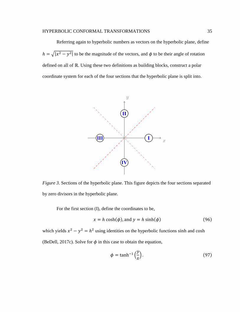
Referring again to hyperbolic numbers as vectors on the hyperbolic plane, define

ℎ = √|𝑥2 − 𝑦2| to be the magnitude of the vectors, and 𝜙 to be their angle of rotation

defined on all of ℝ. Using these two definitions as building blocks, construct a polar

coordinate system for each of the four sections that the hyperbolic plane is split into.

Figure 3. Sections of the hyperbolic plane. This figure depicts the four sections separated

by zero divisors in the hyperbolic plane.

For the first section (I), define the coordinates to be,

𝑥 = ℎ cosh(𝜙), and 𝑦 = ℎ sinh(𝜙) (96)

which yields 𝑥2 − 𝑦2 = ℎ2 using identities on the hyperbolic functions sinh and cosh

(BeDell, 2017c). Solve for 𝜙 in this case to obtain the equation,

𝜙 = tanh−1 (𝑦

𝑥) . (97)


36

This says that 𝜙 = 0 whenever 𝑦 = 0 which graphically means that 𝜙 = 0 along the 𝑥-

axis of the hyperbolic plane in section (I). Given any hyperbolic number 𝑧 = 𝑥 + 𝑗𝑦 in

section (I), convert into polar coordinates to obtain,

𝑧 = 𝑥 + 𝑗𝑦 = ℎ cosh(𝜙) + 𝑗ℎ sinh(𝜙) = ℎ(cosh(𝜙) + 𝑗 sinh(𝜙)) = ℎ𝑒𝑗𝜙. (98)

Thus, in section (I), the polar representation of any number is ℎ𝑒𝑗𝜙.

To construct the polar coordinates for the other three sections, take the

coordinates in section (I) and transform them to fit the other sections. This is done using

the transformation functions 𝑓(𝑧) = 𝑗𝑧, 𝑓(𝑧) = −𝑧, and 𝑓(𝑧) = −𝑗𝑧. Knowing that

𝑓(𝑧) = 𝑗𝑧 acts as a rotation by 90 degrees, 𝑓(𝑧) = −𝑧 acts as rotation by 180 degrees,

and 𝑓(𝑧) = −𝑗𝑧 acts as a rotation by 270 degrees, construct polar coordinates for all of

the hyperbolic plane with the exception of the dividing lines 𝑦 = 𝑥 and 𝑦 = −𝑥.

For section (II), the polar coordinate mapping must be,

𝑧 = 𝑗ℎ𝑒𝑗ℎ = 𝑗ℎ(cosh(𝜙) + 𝑗 sinh(𝜙)) = ℎ(sinh(𝜙) + 𝑗 cosh(𝜙)) (99)

because this is the original polar map transformed with the 𝑓(𝑧) = 𝑗𝑧 transformation.

With this new coordinate map notice,

𝑥 = ℎ sinh(𝜙), 𝑦 = ℎ cosh(𝜙), and 𝜙 = tanh−1 (𝑥

𝑦) . (100)

This means that 𝜙 = 0 along the 𝑦-axis in section (II).

For section (III), the polar coordinate mapping must be,

𝑧 = −ℎ𝑒𝑗𝜙 = −ℎ(cosh(𝜙) + 𝑗 sinh(𝜙)). (101)

This is the original polar map under the 𝑓(𝑧) = −𝑧 transformation. Notice,

𝑥 = −ℎ cosh(𝜙), 𝑦 = −ℎ sinh(𝜙), and 𝜙 = tanh−1 (𝑦

𝑥) . (102)


37

Thus 𝜙 = 0 along the 𝑥-axis in section (III).

For section (IV), the polar coordinate mapping must be,

𝑧 = −𝑗ℎ𝑒𝑗𝜙 = −𝑗ℎ(cosh(𝜙) + 𝑗 sinh(𝜙)) = −ℎ(sinh(𝜙) + 𝑗 cosh(𝜙)) (103)

which implies that,

𝑥 = −ℎ sinh(𝜙), 𝑦 = −ℎ cosh(𝜙), and 𝜙 = tanh−1 (𝑥

𝑦) . (104)

Thus 𝜙 = 0 along the 𝑦-axis in section (IV). Figure 4 summarizes the above results just

derived.

Figure 4. Hyperbolic polar coordinates Example 2. This figure displays the polar

coordinate maps for each section in the hyperbolic plane.

The polar coordinate system is demonstrated in the following example.

Example 2. Consider hyperbolic numbers 2 + 𝑗, −2 + 3𝑗, 1 − 2𝑗, and −2 − 𝑗.

Plot each number in the hyperbolic plane and then convert each number to polar

coordinates and plot them again. First, plot each of the points by writing them as ordered

pairs, i.e. (2, 1), (-2, 3), (1, -2), and (-2, -1). This provides the plot shown in Figure 5.


38

Now write each point in its coordinate system based on which section it resides in.

The point 2 + 𝑗 goes to √3𝑒𝑗(0.55), −2 + 3𝑗 goes to √5𝑗𝑒𝑗(−0.80), 1 − 2𝑗 goes to

− √3𝑗𝑒𝑗(−0.55), and −2 − 𝑗 goes to − √3𝑒𝑗(0.55). Plotting the polar coordinates provides

Figure 6.

Comparing both figures, we see that the points are mapped the same.

Figure 5. Example 2 plot. This figure shows the graphical location of each of the points

in Example 2.

Pairing each of the four polar coordinates in each of the sections together with the

rotation transformations provides full control over the placement of points in the

hyperbolic plane. Now having all the necessary tools, we demonstrate the solution

technique for solving the wave equation in various regions.


39

Figure 6. Hyperbolic polar coordinates Example 2 post-conversion. This figure shows the

values from Figure 5 after they have been transformed via the hyperbolic polar

coordinates.

The Wave Equation Solution Technique

Basic Example Solutions

Here, the solutions to one-dimensional wave equation boundary value problems

are given. The applications of such a problem to physics are not discussed here, but

Motter & Rosa (1998) discuss potential physics implications in their paper on hyperbolic

calculus. Following an example to demonstrate the solution method, a list of

transformation regions will be given to assist in the future study of this solution

technique.

Example 3. Consider the shaded region in Figure 7 defined by the inequality 0 ≥

𝑦 ≥ 𝑥 for 𝑥, 𝑦 ∈ ℝ. Viewing Figure 7 as a vector representation of the hyperbolic


40

number plane, each point (𝑥, 𝑦) in the shaded region can be written as a hyperbolic

number 𝑧 = 𝑥 + 𝑗𝑦.

We will solve the boundary value problem in which the top curve has value 𝜙 =

10 and the bottom curve has value 𝜙 = 0. We have shown that log(𝑤) is ℋ-

differentiable and thus its component functions are solutions to the wave equation.

We can transform the region into the region given by level curves of tanh−1(𝑦/𝑥) via the

transformation function 𝑓(𝑧) = 1/𝑧. Transforming the region, we obtain Figure 8 which

is defined by 0 ≤ 𝑦 ≤ 𝑥.

Figure 7. Example 3 pre-transformation. This figure shows the region that Example 3

seeks to find a solution to the wave equation on.


41

Figure 8. Example 3 post-transformation. This figure shows the region in Figure 7

transformed under 𝑓(𝑧).

Since tanh−1(𝑦/𝑥) is a component function of log(𝑤), it is a solution to the wave

equation. Thus, we can use it as a template solution, plug in the boundary conditions and

solve the following system of equations.

𝐴 tanh−1(𝑦/𝑥) + 𝐵 = 10 𝐴 tanh−1(𝑦/𝑥) + 𝐵 = 0. (105)

Solve for the value of tanh−1(𝑦/𝑥) in both above equations. Note the values will not be

equal because each equation is describing a different boundary. The leftmost equation is

describing the bottom boundary (𝜙 = 10) which is described by the equation 𝑦 = 0. The

rightmost equation is describing the top boundary (𝜙 = 0) which is described by the

equation 𝑦 = 𝑥/2. To find the value of tanh−1(𝑦/𝑥) in the leftmost equation, we use the

following process.

tanh−1(𝑦/𝑥) = 𝑐1 → 𝑦 = tanh(𝑐1)𝑥 =𝑥

2⇒ 𝑐1 = 0.55. (106)

For the rightmost equation,


42

tanh−1(𝑦/𝑥) = 𝑐2 → 𝑦 = tanh(𝑐2)𝑥 = 0 ⇒ 𝑐2 = 0. (107)

Now the system to solve for the solution is,

𝐴(0.55) + 𝐵 = 10 , 𝐵 = 0, (108)

which provides solution,

Φ = 18.18 tanh−1 (𝑦

𝑥) . (109)

Now simply transform this solution back into the starting region,

𝜙 = Φ(𝑓(𝑧)) = Φ (1

𝑧) = −18.18 tanh−1 (

𝑦

𝑥) . (110)

Example 4. Consider the transformation function 𝑓(𝑧) = 𝑗𝑧. Which region would

be mapped into the region solved by Φ = 𝐴 tanh−1(𝑦/𝑥) + 𝐵? To find the solution 𝜙,

take the composition of the transform function and 𝑓 and Φ.

𝜙 = Φ(𝑓(𝑧)) = Φ(𝑗𝑧) = Φ(𝑦 + 𝑗𝑥) = 𝐴 tanh−1 (𝑥

𝑦) + 𝐵. (111)

Thus transforming 𝜙 under 𝑓 is Φ. Figure 9 transformed under 𝑓(𝑧) is Figure 10.

Figure 9. Example 4 region pre-transformation. This figure depicts the region that will

map into Figure 10 under 𝑓(𝑧).


43

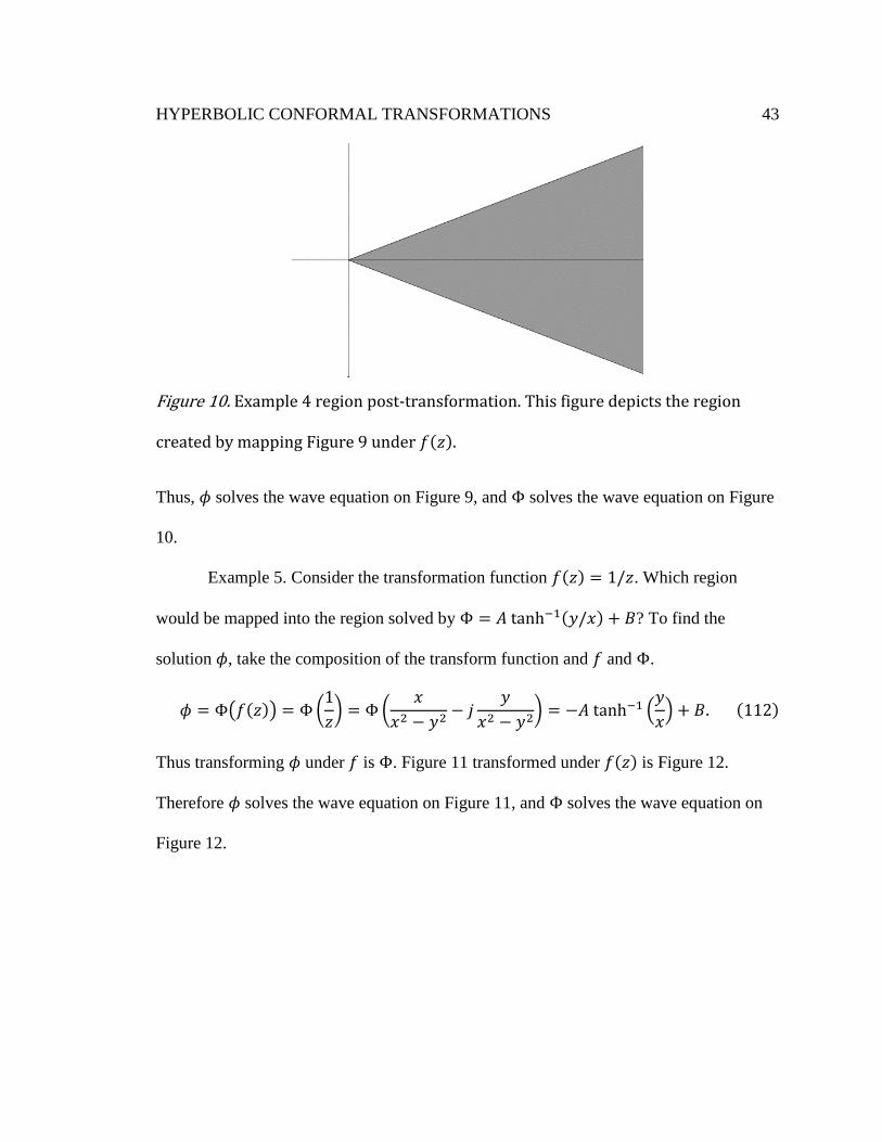
Figure 10. Example 4 region post-transformation. This figure depicts the region

created by mapping Figure 9 under 𝑓(𝑧).

Thus, 𝜙 solves the wave equation on Figure 9, and Φ solves the wave equation on Figure

10.

Example 5. Consider the transformation function 𝑓(𝑧) = 1/𝑧. Which region

would be mapped into the region solved by Φ = 𝐴 tanh−1(𝑦/𝑥) + 𝐵? To find the

solution 𝜙, take the composition of the transform function and 𝑓 and Φ.

𝜙 = Φ(𝑓(𝑧)) = Φ (1

𝑧) = Φ (

𝑥

𝑥2 − 𝑦2− 𝑗

𝑦

𝑥2 − 𝑦2) = −𝐴 tanh−1 (

𝑦

𝑥) + 𝐵. (112)

Thus transforming 𝜙 under 𝑓 is Φ. Figure 11 transformed under 𝑓(𝑧) is Figure 12.

Therefore 𝜙 solves the wave equation on Figure 11, and Φ solves the wave equation on

Figure 12.


44

Figure 11. Example 5 region pre-transformation. This figure depicts the region that will

map into Figure 12 under 𝑓(𝑧).

Figure 12. Example 5 region post-transformation. This figure depicts the region created

by mapping Figure 11 under 𝑓(𝑧).


45

Example 6. Consider the transformation function 𝑓(𝑧) = 𝑧2. Which region would

be mapped into the region solved by Φ = 𝐴 tanh−1(𝑦/𝑥) + 𝐵? To find the solution 𝜙,

take the composition of the transform function and 𝑓 and Φ.

𝜙 = Φ(𝑓(𝑧)) = Φ(𝑧2) = Φ(𝑥2 + 𝑦2 + 𝑗(2𝑥𝑦)) = 𝐴 tanh−1 (2𝑥𝑦

𝑥2 + 𝑦2) + 𝐵. (113)

Thus transforming 𝜙 under 𝑓 is Φ. To find the region where 𝜙 is a solution, we need only

find the inverse of 𝑓 and transform the post transformation region under it. The inverse

function 𝑓−1(𝑧) is seen to be √𝑧. Following a calculation in BeDell & Cook (2017), a

formula for the square root of a hyperbolic number 𝑧 = 𝑥 + 𝑗𝑦 is shown to be,

(𝑥 + 𝑗𝑦)1/2 =1

√2√𝑥 + √𝑥2 − 𝑦2 +

𝑗

√2√𝑥 − √𝑥2 − 𝑦2. (114)

Using this formula, the various points in the post-transformation region shown in Figure

12 can be transformed. First, notice that the top and bottom boundaries of Figure 12 are

described by the set of points 𝛾+ = {𝑘(1 + 𝑗): 𝑘 ∈ 𝑅} and 𝛾− = {𝑘(1 − 𝑗): 𝑘 ∈ 𝑅}

respectively. Under the transformation 𝑓−1(𝑧) = √𝑧 we find that 𝛾+ = {√𝑘/2(1 + 𝑗)} =

𝛾−. Thus, both boundaries are mapped to the same position as the upper boundary with

the length compressed by a factor of √𝑘/2. To study the points between the two

boundaries the polar representation is useful. Recall that in the region being considered,

each point 𝑢 + 𝑗𝑣 can be written ℎ𝑒𝑗𝜙 where ℎ = √𝑢2 − 𝑣2. Each point under 𝑓−1 is

then calculated to be √ℎ𝑒𝑗𝜙 = √ℎ/2(√cosh 𝜙 + 1 + 𝑗√cosh 𝜙 − 1). Points below the

upper boundary 𝛾+ and above the 𝑥 axis are represented by the angle 𝜙1 = cosh−1𝐴 for

some value 𝐴 in the domain of cosh. Similarly, angle 𝜙2 = −cosh−1𝐴 represented points


46

below the 𝑥 axis and above 𝛾−. As cosh is an even function, we have that 𝜙1 = 𝜙2.

Plugging these values into the arbitrary point given above, we find that 𝑓−1 takes points

in Figure 12 and maps them in such a way as to double cover the region between 𝛾+ and

the 𝑥 axis. Figure 13 displays this result.

Figure 13. Example 6 pre-transformation region. Under the 𝑓 = 𝑧2 mapping, this region

would map into the region depicted in Figure 12.

Example 7. Consider the transformation function 𝑓(𝑧) = (𝑗 − 𝑧)/(𝑧 + 𝑗). Which

region would be mapped into the region solved by Φ = 𝐴 tanh−1(𝑦/𝑥) + 𝐵? To find the

solution 𝜙, take the composition of the transform function and 𝑓 and Φ.

𝜙 = Φ(𝑓(𝑧))

= Φ (𝑗 − 𝑧

𝑧 + 𝑗)

= Φ (𝑥2 + 𝑦2 − 1

𝑥2 − (𝑦 + 1)2+ 𝑗

2𝑥

𝑥2 − (𝑦 + 1)2)


47

= 𝐴 tanh−1 (2𝑥

𝑥2 + 𝑦2 − 1) + 𝐵. (115)

Thus transforming 𝜙 under 𝑓 is Φ. After a short calculation, the inverse of 𝑓 is found to

be 𝑓(𝑧) = 𝑗(1 − 𝑧)/(1 + 𝑧). Similar calculations can be made as in Example 6 to find

the region that the inverse function maps the post-transformation region into.

Physics Applications

The examples provided in the previous section pose interesting questions

regarding the physical interpretation of the regions created with the hyperbolic mappings.

What does solving the wave equation bounded by a region mean in physics? The answer

to this question is beyond the scope of this paper, but hopefully, the structures developed

in this paper will assist in furthering that understanding.

Rather than solve the wave equation subject to the boundaries presented above,

consider solving the wave equation subject to two points with fixed values as the

boundary conditions. The solutions will resemble specific waves rather than regions.

Specifically, consider solving the wave equation with unit speed,

𝑢𝑡𝑡 = 𝑢𝑥𝑥 (116)

subject to the boundary conditions 𝑢(0, 𝑡) = 0 and 𝑢(𝜋, 𝑡) = 0. The standard template

solution to this is found through Fourier Analysis to be,

𝑢(𝑥, 𝑡) = ∑ 𝑎𝑛sin(𝑛𝑥)cos(𝑛𝑡)

∞

𝑛=1

+ 𝑏𝑛sin(𝑛𝑥)sin(𝑛𝑡). (117)

For further study into Fourier Analysis, see the works by Gustafson (1980), Haberman

(1998), Logan (2015), and Weinberger (1995).


48

In general, the standard solution can fit any physically reasonable boundary

condition and to solve, the coefficients 𝑎𝑛 and 𝑏𝑛 must be found. A similar template

solution can be found for the hyperbolic numbers. This construction paired with the

mapping technique described in previous sections allows for interesting and exotic

solutions to the wave equation to be found with minimal effort. Consider the function,

𝑓𝑛(𝑧) = sin(𝑛𝑧) (118)

with hyperbolic number 𝑧 = 𝑥 + 𝑗𝑡 and 𝑛 an integer. To utilize 𝑓, it must be broken into

its component functions. Utilizing results on the sin function from BeDell (2017c) we

find,

𝑓𝑛(𝑧) = sin(𝑛(𝑥 + 𝑗𝑡))

= sin(𝑛𝑥 + 𝑛𝑗𝑡)

= sin(𝑛𝑥)cos(𝑛𝑗𝑡) + sin(𝑛𝑗𝑡)cos(𝑛𝑥)

= sin(𝑛𝑥)cos(𝑛𝑡) + 𝑗 sin(𝑛𝑡)cos(𝑛𝑥). (119)

It can be shown that 𝑓 is ℋ-differentiable and thus its component functions are solutions

to the wave equation with unit speed. Notice the real component of 𝑓 is the same term

associated with the 𝑎𝑛 coefficient in the standard Fourier template solution shown above.

Similarly, consider the function,

𝑓𝑛(𝑧) = cos(𝑛𝑧)

= cos(𝑛(𝑥 + 𝑗𝑡))

= cos(𝑛𝑥 + 𝑛𝑗𝑡)

= cos(𝑛𝑥)cos(𝑛𝑗𝑡) − sin(𝑛𝑥)sin(𝑛𝑗𝑡)

= cos(𝑛𝑥)cos(𝑛𝑡) − 𝑗 sin(𝑛𝑥)sin(𝑛𝑡). (120)


49

Notice here that the 𝑗 component of 𝑓 is the same term associated with the 𝑏𝑛 coefficient

in the standard Fourier template solution. Considering both functions, sin(𝑛𝑧) and

cos(𝑛𝑧) together, a hyperbolic Fourier template is proposed to be,

𝑢(𝑥, 𝑡) = ∑ 𝑗

∞

𝑛=1

𝐴𝑛sin(𝑛𝑧) + 𝐵𝑛cos(𝑛𝑧). (121)

Using the hyperbolic Euler's equation, this can be simplified further to,

𝑢(𝑥, 𝑡) = ∑ 𝑗

∞

𝑛=1

𝐴𝑛sin(𝑛𝑧) + 𝐵𝑛cos(𝑛𝑧) = ∑ 𝐶𝑛𝑒𝑗𝑛𝑧

∞

𝑛=1

. (122)

Consider the initial problem, solving the wave equation of unit speed with the

boundary conditions 𝑢(0, 𝑡) = 0 and 𝑢(𝜋, 𝑡) = 0. By observation, the solution can be

seen to be,

𝑢(𝑥, 𝑡) = sin(𝑥)cos(𝑡). (123)

Looking more closely, this solution is the real component of the function 𝑓𝑛(𝑧) =

sin(𝑥 + 𝑗𝑡) = sin(𝑧). Using this as the region to be mapped into, various transform

functions can be analyzed to discover new and interesting solutions to the wave equation.

Recall that the solution 𝜙 can be found via the composition of Φ and 𝑓, the

transform function. What follows is a series of examples deriving new solutions to the

wave equation. What these solutions represent in physics is unknown, but the strong

connection to Fourier analysis suggests the connection is significant. Let Φ = sin(𝑤) for

hyperbolic number 𝑤 = 𝑢 + 𝑗𝑣. Breaking Φ into its component functions reveals,

Φ = sin(𝑢)cos(𝑣) + 𝑗 sin(𝑣)cos(𝑢). (124)

Example 8. Consider the transformation function 𝑓(𝑧) = 𝑗𝑧. To find 𝜙 take,


50

𝜙(𝑧) = Φ(𝑓(𝑧))

= Φ(𝑗𝑧)

= Φ(𝑡 + 𝑗𝑥)

= sin(𝑡)cos(𝑥) + 𝑗 sin(𝑥)cos(𝑡). (125)

The equation 𝜙 is a solution to the wave equation subject to the boundary conditions


Example 9. Consider the transformation function 𝑓(𝑧) = 𝑧2. To find 𝜙 take,

𝜙(𝑧) = Φ(𝑓(𝑧))

= Φ(𝑧2)

= Φ(𝑥2 + 𝑡2 + 2𝑗𝑥𝑡)

= sin(𝑥2 + 𝑡2)cos(2𝑥𝑡) + 𝑗 sin(2𝑥𝑡)cos(𝑥2 + 𝑡2). (126)



Example 10. Consider the transformation function 𝑓(𝑧) = (𝑗 − 1)/(1 + 𝑗). To

find 𝜙 take,

𝜙(𝑧) = Φ(𝑓(𝑧))

= Φ (𝑗 − 1

1 + 𝑗)

= Φ (𝑥2 + 𝑦2 − 1

𝑥2 − (𝑦 + 1)2+ 𝑗

2𝑥

𝑥2 − (𝑦 + 1)2)


51

= sin (𝑥2 + 𝑦2 − 1

𝑥2 − (𝑦 + 1)2) cos (

2𝑥

𝑥2 − (𝑦 + 1)2)

+ 𝑗 sin (2𝑥

𝑥2 − (𝑦 + 1)2) cos (

𝑥2 + 𝑦2 − 1

𝑥2 − (𝑦 + 1)2) . (127)



Future Research

There are many open questions regarding the hyperbolic number plane, but this

paper has hopefully exemplified that these questions are worthy of being answered. An

important next step would be to discover a hyperbolic Möbius transformation which

would allow more complicated examples to be solved and find more meaningful

transformations useful in physics. Another useful area to continue studying would be the

physical interpretation of one-dimensional wave equation boundary value problems.

Utilizing the Hyperbolic Fourier construction allows for the solving of highly exotic

wave equation problems. Interpreting what these exotic solutions mean in physics would

be a worthy pursuit. The final section of this paper is meant to be used as a guide for the

future study of solutions to the wave equation. The examples presented here are not an

exhaustive list but serve as a good foundation for more complicated solutions.


52

References

BeDell, N. (2017a). Doing algebra in associative algebras. Unpublished manuscript.

BeDell, N. (2017b). Logarithms over associative algebras. Unpublished manuscript.

BeDell, N. (2017c). Generalized trigonometric functions over associative algebras.

Unpublished manuscript.

BeDell, N., & Cook, J. S. (2017). Introduction to the theory of A-ODE’s. Unpublished

manuscript.

Briggs, W., Cochran, L., Gillett, B., & Schulz, E. (2013). Calculus for scientists and

engineers. New York: Pearson Education, Inc.

Brown, J. W., & Churchill, R. V. (2009). Complex variables and applications. New

York: McGraw-Hill.

Catoni, F., Boccaletti, D., Cannata, R., Catoni, V., & Zampetti, P. (2011). Geometry of

Minkowski space-time. Berlin: Springer-Verlag.

Cook, J. S. (2017). Introduction to A-calculus. Unpublished manuscript.

Cook, J. S., Leslie, W. S., Nguyen, M. L., & Zhang, B. (2013). Laplace equations for real

semisimple associative algebras of dimension 2, 3 or 4. Springer Proceedings in

Mathematics & Statistics, 64, 67-83. doi:10.1007/97814614933278.

Curtis, C. W. (1984). Linear algebra, an introductory approach. New York: Springer-

Verlag.

Edwards, C. H. (1994). Advanced calculus of several variables. New York: Dover

Publications, Inc.


53

Gaudet, E., Foret, J., Olsen, S., & Austin, W. (n.d.). Mobius transformations in

hyperbolic space. Retrieved from https://www.math.lsu.edu/system/files/Final

Draft.pdf

Gustafson, K. E. (1980). Introduction to partial differential equations and Hilbert space

methods. New York: John Wiley & Sons, Inc.

Haberman, R. (1998). Elementary applied partial differential equations with Fourier

series and boundary value problems. Upper Saddle River: Prentice-Hall, Inc.

Logan, J. D. (2015). Applied partial differential equations. Switzerland: Springer

International Publishing.

McInerney, A. (2013). First steps in differential geometry, riemannian, contact,

symplectic. New York: Springer Science+Business Media.

Motter, A. E., & Rosa, M. A. F. (1998). Hyperbolic calculus. Advances in applied

Clifford algebras, 8(1), 109-128. doi:10.1007/BF03041929

Saff, E. B., & Snider, A. D. (2016). Fundamentals of complex analysis with applications

to engineering, science, and mathematics. Tamil Nadu: Dorling Kindersley India

Pvt. Ltd.

Salas, S., Hille, E., & Etgen, G. (2007). Calculus one and several variables. Hoboken:

John Wiley & Sons, Inc.

Sobczyk, G. (1995). The hyperbolic number plane. The College Mathematics Journal,

26(4), 268-280. doi:10.2307/2687027.

Weinberger, H. F. (1995). A first course in partial differential equations with complex

variables and transform methods. New York: Dover Publications, Inc.

digital commons - liberty university research

Documents