digital communications -...
TRANSCRIPT

Chapter 13
Digital Communications
To this point in time (2003), when one thinks of optical communication, one generally thinks of fiber opticalcommunication and the telephone network. Indeed, to the present (although the situation is evolving),the phone companies (telecos) have been the largest users of fiber optic technology. This form of opticalcommunication is an archetypical form of digital communication using optics. There are other applicationsof digital communications using optics; among others, there is data communications (datacom). We’ll try tokeep the discussion in this chapter general, but a number of examples will come from telecommunications.There are good reasons for why the telephone companies went so rapidly and completely over to fiber atthe same time they were trying so hard to convert to digital transmission as well as for why fiber optictechnology proved so powerful in carrying the digital implementation. To put audio frequency informationon a transmission line requires one to use some amount of bandwidth. The ear of a young (25 years oryounger) musician will have a frequency response from perhaps 20 Hz to 20 KHz. Things over about 10 KHzby themselves are, however, probably not too pleasant to hear, like chalk on a blackboard or a misguidedcolatura soprano. There could be pleasant sounds, however, with lower center frequencies that includefrequencies in the 10–20 KHz band as overtones to fill out the sound. To understand somebody speakingnormal everyday conversation, such high frequencies are unnecessary. It was therefore arbitrarily decidedsomewhere a long ways back that a 4-KHz bandwidth was sufficient for direct transmission of a voice.Therefore, in the mouthpiece of a telephone there is a diaphragm which is shaken by the acoustic wavesemanating from the vocal cords of the caller that converts the waves to an electrical signal on a wire thatwill respond as linearly as possible to the shaking audio frequency spectra up to a maximum frequency of4 KHz. In the earpiece of the telephone there is an inverse-purposed transducer which, for a 0–4 KHz inputelectrical signal, generates a 0–4 KHz output audio signal.
Once we can convert an audio signal to an electrical signal and vice versa, we need to get it from one placeto another. The original telephone system (1870s) did this first with a circuit switching system employing asingle-conductor telegraph wire until the adoption of the less noisy twisted-pair wire medium (early 1900s).The idea was that, when one dials the number of another end user, the dialing sequence will then havethe effect of throwing (or, originally, of having operators throw) a number of switches until direct pathsfor both transmission and reception are set up between the users. Their connection then really looks like acircuit. As was mentioned, the connection medium of choice was, from the early 1900s through the 1960s,twisted-pair—that is, two insulation-coated wires literally just twisted around each other with one carryingthe signal and the other acting as a local ground. (Twisted pair is still the medium which takes phone callsfrom drop boxes on the curb into the house, but it is questionable even in this application that it is anylonger the medium of choice, but rather that it’s just too expensive to exchange it for fiber.) Despite thelongness of the wavelength at 4 KHz, the cable pathlength could be quite long as well in the trunk lineapplication—i.e. between local offices—so that the inclusion of the ground wire along next to the signalwire is just to insure that the signal always sees the desired ground at a subwavelength distance, fixing thedirection of the Poynting vector to point in the direction of the wire axis which is the desired directionof propagation and thereby insuring one against such things as spurious reflections. (See the discussion insection 4.4 of Chapter 4 or in the Introduction to Part IV.)
1

CHAPTER 13. DIGITAL COMMUNICATIONS 2
Already by the 1950s, some problems were arising with such a transmission system. A major one wascapacity. The telephone system, like any system tied in some way to population, is plagued with theproblem of exponential growth. (The number of applications being developed is probably also increasingexponentially, at least at the present time.) The circuit-switched system was, to say the least, inefficient, aslarge numbers of operators were needed to plug wires into large switchboards (manually operated crossbarswitches). Further, with each line carrying but one telephone call, the quantities of wire involved in thesystem were rapidly becoming appalling. Of course, the real problem with the quantity of wire was that ofso-called right of way. This is the reason that time-division multiplexing (TDM) was first introduced in circa1962. However, the twisted pair medium was not especially upgradable. The phone companies could onlycontrol so many ducts underground and string so many wires on telephone poles above ground. At somepoint, the space for twisted-pair wire would simply be used up, and further network growth would necessarilyhave to be halted. It has also been touted that the cost of right of way is so expensive as to completelyswamp all other costs, although this is probably somewhat of an overstatement. Installation of cable intoducts is not inexpensive either. Further, there really was no cost issue associated with telecommunicationsper se until the early 1980s when the phone companies, which were mostly government-regulated and, inmany countries, wholly government-owned and operated monopolies, began to be deregulated. Slowly butsurely, market forces are now causing companies to take a new and different look at cost.
The demonstration of a transistor in 1947 (Bardeen and Brattain 1948; Schockley 1949) led to a succes-sion of developments in electronics. By the early 1960s, integrated circuit technology had already becomesufficiently advanced that it was possible to construct digital switches—that is, switches which could beactivated by “control bits” included on a digitally encoded information stream incident on the switch. Theera of automatic routing was upon us. However, digital signals, as we will presently discuss, require signif-icantly more bandwidth than do their analog counterparts, and the switches required that the signals bedigital. Digitally coding a 4-kHz analog channel requires roughly 64 kbps, sixteen times the rate—not tospeak of the extra bandwidth required to get edges on these bits. Automatic routing cried out for a digitalsolution, as did the mass-of-wire problem for a different reason. Including more and more wires, each fora single conversation, is a technique known as space-division multiplexing (SDM). In the ‘Fifties and intothe ‘Sixties, SDM was both the only solution and the problem. With digital encoding, however, anotherform of multiplexing can be employed, that of time-division multiplexing (TDM). In TDM, one takes, forexample, two streams both at the same rate of b bps. By halving the length of each bit and interleaving thebits, one can generate a composite stream of 2b bits in the same time period—but with the cost associatedwith doubling the bandwidth of the signal. The first thing that was done with telephone conversations wasto combine 24 conversations at a time to generate a composite rate of roughly 1.5 Mbps. (This rate is notquite 24 times the single conversation rate, as there are techniques to correct for transmission errors byincluding a few extra so-called parity bits. In a system which allows high latency—i.e., where some simpleprocessing can be carried out on the signal before completing transmission—some form of parity correctioncode is practically always employed, as the gain in bit error rate can be dramatic. Generally, if latency isan issue, the only way to lower the bit error rate is to raise the signal-to-noise level through increasing thetransmitted power.) This rate was called digital signal 1 (DS-1), and its original implementation was calledT1, although now the terms DS-1 and T1 are used interchangeably. It was this trunk line implementationwhich proved to be the first triumph of fiber optics. The real problem with the wire implementation of thisrate wasn’t that it could not be done. (Twisted-pair was still used in the local loop, whereas coaxial cablewas generally being used in the trunk lines where the TDM was taking place.) It could if signal-regeneratingrepeaters were to be placed each two kilometers. The problem was that the rate could not be upgraded asthe subscribership increased without reducing the repeater spacing. The problem was one of bandwidth.The wire was just too dispersive at rates higher than 1 Mbps—and these rates were to become necessary.Today’s long-line standards are dictated by the synchronous optical network (SONET) standard, which, to-gether with the European synchronous digital hierarchy (SDH), are the international standards which allowfor seamless interconnection over transoceanic links, for example. The standard dictates that TDM ratescan increase by factors of four from 565 Mbps to 2.5 Gbps to 10 Gbps to 40 Gbps, etc., and prescribesthe interleaving of the bit pattern and parity codes. These are long-line rates, but an article by Personick(1992) indicates that telecommunication companies have not-so-long-term plans to form the local loops intological buses with TDM rates of up to 10-Gbps SONET links in order to be able to supply high-resolution

CHAPTER 13. DIGITAL COMMUNICATIONS 3
video to businesses. (That this increase to widespread use of 10-Gps is taking some time again has to dowith cost. As most telecos no longer have in-house circuit-making facilities, they need to buy from majorsuppliers. Major suppliers don’t really want to make a major effort until there is widespread demand. Thetotal demand for a certain circuit from the telecommunications industry is a drop in the bucket comparedto, for example, the demand for components from the personal computer market.) This 10-Gbps discussedtrunk rate is a far cry from the 1.5-Mbps non-upgradeable rate of the mid ‘60s. How did we get there?
It was fortuitous circumstances which so rapidly brought optical communications to the telephone net-work. The first work on waveguides really dates back to Rayleigh (1897) and shortly after to Sommerfeld(1899), although complete solutions of the fully dielectric waveguide problem were not really given in asuccinct form until the work of Hondros and DeBye (1910) in 1910. Their results were pretty well verifiedby microwave measurements in 1916 (Zahn 1916) and 1920 (Schriever 1920). There really wasn’t muchmore work in this area until after Maimon’s demonstration of the ruby laser in 1960 (Maimon 1960), whichprompted a study of dielectric optical fibers by Snitzer in 1961 (Snitzer 1961a). A problem, though, withSnitzer’s fiber was that the loss was so high (> 10 dB/cm) that it transmitted almost no light over anyappreciable distance, and this actually prompted him to develop (Snitzer 1961b) the rare-earth-doped fiberamplifier in 1963 (Koester and Snitzer 1963). Even with that improvement, fiber was a long way frompractical in those days. The laser demonstration also prompted various groups to demonstrate electricallypumped semiconductor lasers in 1961 (Basov et al 1961, Hall et al 1962, Nathan et al 1962), albeit all withthe drawback that these lasers could not be operated at room temperature or anywhere near it. These earlydemonstrations caught the attention of the telecos, but the technology was still far from the applicationstage. The phone companies worldwide during these years were frantically searching for a solution to theircapacity quandary. The solution to their problem appeared in 1970 with, on the one hand, the demonstrationof low-loss (< 100 dB/km) optical fiber at Corning Glass Works (Kapron et al 1970) and the demonstrationof room-temperature semiconductor laser operation by several groups that same year (Alferov et al 1970,Hayashi and Panish 1970). In 1975, trunk lines (with 2-km repeater spacing) began to be installed withmultimode fiber (bandwidth of > 100Mbps·km), which proved to be upgradeable to DS-3 rates (64 Mbps)and therefore to solve the immediate problems of the crowding of rights of way and nonupgradeability of coaxand twisted pair solutions. Although most predictions were that fiber would then find its way into the localloop and eventually into the home, things actually went the other way. Single-mode fiber (pulse-spreadingof roughly 1 ps/km/nm sourcewidth and loss of 0.5 dB/km at 1.3µm and of 0.2 dB/km at 1.55µm) andsingle-mode semiconductor lasers (spectral widths 0.04 nm) by roughly 1980 allowed fiber to go into longlines (20-km repeater spacing, highest possible bandwidth with greater than 100µW power output). Thefiber proved so advantageous in the long-line applications that essentially all worldwide long lines have beenshifted to fiber at present, and several new transoceanic links have been implemented with several moreplanned.
As the above has outlined, optical fiber may not have been ideally suited to the telephone network,but fiber optic communications technology arrived at the right time to take over the application. Further,since telephone network subscribership is tied to population dynamics as well as the computer-supporteddata age, the growth has been and will continue to be exponential. Digital optical communications is hereto stay, and such is a prime motivation for this chapter. This is not to say that other applications arenot constantly arising for fiber optics and even free-space optical technology. At that point in the ‘80swhen optical communications was truly making its debut in such a big way that those in the financialmarkets began to take note, there were numerous predictions of how rapidly fiber optic technology wouldexpand into other markets. These predictions, for the most part, were off the mark. Expansion to diverseapplications has been much more gradual than was generally thought—and basically for good reason. Thetelecommunications industry, which originally began the widespread deployment of fiber in their network,initially gave no thought to the problem of cost. Monopolies don’t need to consider cost and could alwaysexplain the cost as being part of the problem of right of way and argue for rate increases. For fiber tofind widespread use in electronics, the technology will need to become cheap. The early telecommunicationssolutions cannot be used, as they are anything but cheap. The situation is presently evolving. This evolutionis a major reason why I have tried to keep the analysis of this chapter as general as possible. The digitaloptical communications systems of the future and the problems that arise in their implementaion may havelittle in common with the telecommunication problems of yesterday and today.

CHAPTER 13. DIGITAL COMMUNICATIONS 4
Figure 13.1: Schematic depiction of an information-bearing process.
This chapter is organized as follows. The next section will be given to a discussion of information theoryfor the purposes of discussing signal coding and recovery. Section 13.2 will be given to a discussion ofdetection and estimation theory and construction of optimal decision circuitry. Section 13.3 will discussclock recovery and the effect of timing errors on signal-to-noise ratios. Section 13.4 will discuss a techniquefor taking into account propagation effects on the information stream.
13.1 Some Information Theory
Although the world is a continuous analog one, first Whittaker (1915) and independently Nyquist (1928) andthen Shannon (1948) showed us that any analog piece of information has a completely retrievable sampledrepresentation. The sampled pulse heights can be quantized and/or digitized then to form a discrete sampledrepresentation of a continuous analog signal. Transmission in a digital representation can be advantageous.A primary reason for this is a “recognizability” property of a digital transmission. Instead of having torecognize heights and shapes accurately, with a digital signal one needs only to decide after detecting anedge whether the signal is on or off. This makes almost perfect reconstruction a possibility. Further, itmakes almost perfect reconstruction possible with inexpensive digital electronics. The data streams are alsoquite compatible with the signals in digital processors, which are beginning to appear everywhere and withwhich we would like to be able to communicate easily.
13.1.1 Information and Signal Entropy
We have talked about the fact that we want to insert information into one end of the system and hopefullyget something similar out at the other end. Without being able to quantify information, it will be hard toreally evaluate how well we are achieving what we set out to achieve. In this subsection, we will first quantifywhat we mean by information and how to resolve it, and then we’ll see how to code information for optimumpractical reconstructability. As information is easier to quantify in digital transmission systems, we will usea digital yardstick to quantify all information. (Actually, all information is analog. Digital is really just atheoretical construct for quantifying information and coding it.) This will also allow us to appreciate thedistinctions between analog and digital transmission and reception.
Let’s assume that we have a timeline, and at each of a set of discrete times ti an event Ri takes place,as is schematically depicted in Figure 13.1. Let us further assume that each event Ri can have ni distinctoutcomes. We would like to be able to quantify how much information is contained in each of the events Ri.
We could redepict the situation of Figure 13.1 as a network. At each event Ri, a distinct outcome xij
which is one of the ni alternatives is revealed, sketching out a path through the network. Clearly, the totalnumber of possible paths is some measure of the system complexity and must be related to the informationcontained. The total number of paths P must just be the product of the ni, or
P =M∏i=1
ni. (13.1)
We would assume that what we mean by information is that, at each ti, we are supplied with an“additional” piece of information. By additional, we naturally mean that the information should add—i.e., really be independent. The expression of (13.1) has products, not additions. To make the products into

CHAPTER 13. DIGITAL COMMUNICATIONS 5
Figure 13.2: Schematic depiction of an information-bearing process as an ensemble of paths through anetwork.
additions, we need to take a logarithm, or
I =∑
Ii =∑
ln ni. (13.2)
If the outcomes at ti were all equally likely, then we could write that the probability of the jth outcome atthe ith event, pij , is equal to
pij =1ni
, (13.3)
and we could write thatIij = − log pij . (13.4)
That is, the information associated with the jth outcome at the ith event is given by the negative logarithmof the inverse probability of the jth outcome at the ith event. Generally, what an information theorist wouldsay is that there is an a priori uncertainty U associated with the outcome xij , which occurs with probabilitypij , such that
U(xij) = − log pij . (13.5)
If we then measure xij , we say that we have gained a quantity of information
I(xij
∣∣xij) = U(xij), (13.6)
where the x|y notation is read “x given y” and denotes a conditional probability, as we’ll discuss more whenwe come to Baye’s rule in the next subsection. That is, given that we measure xij , there is no uncertaintyleft. If pij is small, it is not very likely that there is a large uncertainty in it occurring and, if it does occur,that is a significant amount of information. If it were a probability 1 event—one that always occurs—thereis no information in measuring it, as there is no uncertainty in its occurrence. In general, we won’t measurexij but instead some yij , even if xij was the symbol sent, as there is always noise present in the channel. Ingeneral, we could say that
I(xij
∣∣yij) < U(xij), (13.7)
but this is the stuff of section 2 of this chapter, where we’ll consider detection theory. For the present, wewant to define a quantity which we can associate with the event Ri at ti, unlike the information which isassociated with the individual outcomes xij of the event Ri. This quantity is the entropy, which we defineas an expectation of the uncertainty
Hi = E[U(xij)
](13.8)
over the set of ni outcomes which, for discrete events xij , we could express as
Hi = −K∑
j
pij ln pij , (13.9)

CHAPTER 13. DIGITAL COMMUNICATIONS 6
Figure 13.3: Plot of the entropy of a single bit as a function of the probability of the bit being on.
where K is some normalization constant. We generally fix the normalization constant by arguing that theentropy associated with a maximally uncertain binary bit be equal to unity. That is, we can write theentropy of a binary bit as
H
K= −p0 ln p0 − p1 ln p1. (13.10)
Usingp0 = 1 − p1, (13.11)
we can further writeH
K= −(1 − p1) ln(1 − p1) − p1 ln p1, (13.12)
which is plotted in Figure 13.3. We see that the maximum is obtained for
p0 = p1 =12
(13.13)
and has the value ln 2. Then, using
K =1
ln 2, (13.14)
we find thatHi = −
∑j
pij log2 pij (13.15)
in order to have bit normalization.An interesting point is that there is a definite relation between signal entropy and the thermodynamic
type of entropy we are used to. As we will soon see, the only difference between them is the normalizationconstant. Let’s consider that there is a system with a density of states as a function of energy that we willcall D(E) and that it is at a temperature T . For a macroscopic system, the number of available states at agiven energy tends to be extremely large, as this number will tend to grow as a factorial of the number ofparticle states accessible. As the average phonon energy at T is kBT and therefore the total system energymust be NkBT where N is the total number of particles, the system is free to make transitions betweenstates with energies ranging from roughly E − kBT/2 to E + kBT/2 by exchanging phonons with its thermalreservoir, and in fact this is the way that the system and reservoir stay in equilibrium. The total number ofstates g(E) accessible to the system is therefore
g(E) = D(E) dE , (13.16)
where the dE is the energy interval. (As it turns out, D(E) grows so rapidly with particle number that, formacroscopic systems, the size of dE is not too important—i.e. whether it is kBT or something else—as the
CHAPTER 13. DIGITAL COMMUNICATIONS 7
D(E) grows as a factorial of the number of particles and the total energy is linear in the total number ofparticles. That is to say that E/dE is infinitesimal compared to D(E) for a macroscopic system.) Now let’ssay that we have M systems, each with an accessible number of states gi. Then the total number of statesaccessible to the composite system will be
gtot =M∏i=1
gi. (13.17)
In order that the entropy of the systems add, we need to define the entropy of a system by
S = K ln g. (13.18)
The constant K can be determined from the classical definition of temperature—that is, the inverse of thetemperature is equal to the partial derivative of the entropy with respect to energy,
1T
=∂S
∂E . (13.19)
To derive this relation, let’s say that we place two systems, 1 and 2, in thermal contact such that they areat different temperatures T1 and T2 but can exchange energy to obtain thermal equilibrium—that is, a statein which T1 = T2 = Teq. The total number of states available to the composite system will be
gt(E) =∫
g1(E − E ′)g2(E ′) dE ′. (13.20)
In order to find out the equilibrium distribution of energy between the two systems, we need to find the E ′
which maximizes the integral. Writing
dgt(E) =∂g1
∂E1g2 dE1 + g1
∂g2
∂E2dE2 = 0, (13.21)
where we must have thatdE1 = −dE2, (13.22)
we find immediately that, at equilibrium,
∂ ln g1
∂E1=
∂ ln g2
∂E2, (13.23)
which in turn gives that∂S1
∂E1=
∂S2
∂E2. (13.24)
However, the left-hand side is a property of system 1 alone, and the right-hand side is a property of system 2alone, but they are properties that approach each other and become equal at thermal equilibrium. This isa property of the temperature as well. Identifying the terms in (13.24) with subsystem temperatures gives,as a definition,
1T
=∂S
∂E . (13.25)
For this to be true dimensionally, we see that the entropy here would have to have dimensions of en-ergy/temperature. As the logarithm of the number of states is dimensionless, we would need the constant Kto have these dimensions. There is just such a fundamental constant with those dimensions. It is Boltzmann’sconstant kB. Indeed, if we set
S = kB ln g, (13.26)
we find that (13.25) holds experimentally. Of course, we could have written (13.14) as
1kBT
=∂S
∂E , (13.27)
CHAPTER 13. DIGITAL COMMUNICATIONS 8
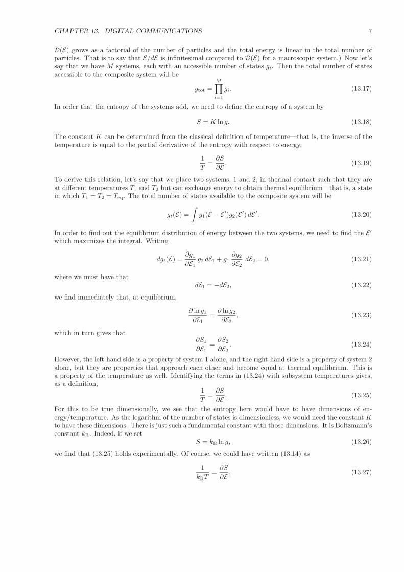
Figure 13.4: An archetypical bandlimited spectrum.
and then the entropy would be dimensionless. It is hard to find a statistical thermodynamics book thatdoesn’t use dimensionless entropy and temperature in units of energy. The important thing about (13.26)really is the ln. The natural logarithm is the natural function to be used with physical entropy, unlike thelog2 in the bit-normalized communications entropy. There is still another difference; however, we’ll soon seethat it is illusory. The communications entropy is defined as an expectation. Well, the physical entropyreally should also be defined as an expectation, as the number of states in the system fluctuates with thefluctuating energy. We could as well write (13.26) as
S = −kBE[ln g(E)
], (13.28)
which in turn could be written asS = −kB
∫p(E) ln p(E) dE . (13.29)
This discussion only serves to reinforce our earlier discussions on the origin of noise. Basically, noise isinformation—but information in such great quantities about so many things that we don’t need to knowthat it becomes an irritant. Even the mathematics reiterates this point. Let’s now return to our discussionof signal information.
13.1.2 The Sampling Theorem
How is it that one can show that each bandlimited analog signal has an invertible sampled representation?Consider an analog signal f(t) which has a Fourier spectrum F (ω) defined by
F (ω) =
∞∫−∞
dt′e−iωt′f(t′), (13.29)
which might appear as in Figure 13.4. The bandlimited aspect should not be considered as especially limiting,as all circuits and systems have finite bandwidth, and therefore any signal will cease to have spectral contentabove some cutoff frequency. What happens when we sample such a signal at fixed intervals?
Let’s say that we have a perfect sampler, such as is depicted in Figure 13.5. Out of the sampler comes asignal which is a set of samples which we will denote by fs(t), where
fs(t) = f(t)p(t), (13.30)
where p(t) is a periodic sampling function with a period T . The situation may be as depicted in Figure 13.5.Because the p(t) is periodic in T , we can write it as a Fourier series:
p(t) =∑
anei 2πT nt. (13.31)

CHAPTER 13. DIGITAL COMMUNICATIONS 9
Figure 13.5: Schematic depiction of (a) a signal, (b) a sampling function, and (c) the sampled signal.
If we then take a Fourier transform of fs(t),
F[fs(t)]
=
∞∫−∞
df ′e−i2πft′fs(t′), (13.32)
we see thatFs(ω) =
∑n
an
∫dt′ e−i2π(f− n
T )t′f(t′), (13.33)
which, from our earlier definition of F (ω), is just
Fs(ω) =∑
n
anF (ω − nωs), (13.34)
where the ωs can be defined by
ωs =2π
T. (13.35)
The situation is as depicted in Figure 13.6.

CHAPTER 13. DIGITAL COMMUNICATIONS 10
Figure 13.6: Sketch of the spectrum of a sampled version of the function whose spectrum appears in Fig-ure 13.1.
Figure 13.6 is really the proof of the Whittaker-Shannon sampling theorem and gives us the so-calledNyquist rate. The idea is that, if ωs is greater than twice ωc, then each bump on the plot of Fs(ω) containsall of the necessary spectral information to reconstruct f(t). If we define the bandwidth B of the signal tobe the cutoff frequency—that is, ωc/2π, then the condition for sampling to be recoverable is
T <1
2B, (13.36)
or that the highest frequency to be preserved must be sampled twice per period. This rate of 2B is calledthe Nyquist rate.
13.1.3 Channel Capacity
Now let’s give some consideration to channel capacity given that we have now defined a transmission systemwhere we transmit a representation of a continuous signal as pulse amplitudes where we need to transmit atleast two of these pulse amplitudes per signal period. One could ask how much information we can get fromthis sampled signal. Let’s consider the digital bit stream depicted in Figure 13.7. How rapidly is informationbeing transmitted here? Each bit has an information content (entropy) of 1, and they come at a rate of1/τinfo, which says that the rate is indeed 1/τinfo. Oftentimes we define a channel capacity C by
C =1
τinfolog2 n, (13.37)
where n is the number of levels, which for binary is 2, whereas for analog it is big but never really infinite.That is to say that we really can’t choose n arbitrarily large, as we know that the world is a noisy place. Thechannel capacity should be the quantity of information which can be sent and received. If we were to choosen too large, we could not distinguish between levels at the receiver. There is some maximum obtainableinformation flow given a channel characteristic. A real signal may well appear as depicted in Figure 13.8.In the channel capacity formula, one can define the number of levels n to be the average signal level dividedby the level spacing a, and clearly the minimum level spacing a must just be some constant times the noiseσ, or
n =P
κσ, (13.38)
which is the same thing as
n =SNR
κ, (13.39)

CHAPTER 13. DIGITAL COMMUNICATIONS 11
Figure 13.7: A possible signal containing a bit stream.
Figure 13.8: A bit stream corrupted by noise.
where SNR is the signal-to-noise ratio—that is, the ratio of the average signal power to the rms Gaussiannoise power in the frequency range extending to τ⊥
info. Shannon (1959) was able to show theoretically thatthe constant could be as small as SNR/(1+SNR) for additive bandlimited Gaussian noise—that is, that thelevel spacing could be equal to the RMS noise level. With this proviso, one can still write that
C =1
τinfolog2(1 + SNR) (13.40)
as the ultimate limit of channel capacity when using pulse amplitude modulation with the optimal number oflevels for a given SNR. Note that, from this, the capacity of the channel can be increased through increasingeither the bandwidth or the SNR. The SNR is a less efficacious way to go, though, as it must increaseexponentially for a linear increase in capacity. To decrease τinfo while keeping the SNR constant requiresonly a linear increase in signal power. Now, even if one could achieve the level spacing of SNR/(1 + SNR),if one were to increase the SNR it would require redesigning encoder, receiver, and decoder for a differentnumber of levels. No one has ever been able to even nearly achieve the channel capacity of (13.40) in practice,and Shannon’s proof was nonconstructive, leaving no hint of how the optimum could be achieved.
The technique that we have described above whereby we store information on the amplitudes of pulsesis called pulse amplitude modulation or PAM. Despite the hope held out by the channel capacity theorem, itis not really a very good technique practically. What is more generally done is to first do a sampling, thenquantize the amplitudes of the samples into 2n levels, and then code the levels into binary (on and off, forexample) pulses. For example, to code into sixteen levels will require a four-bit (24 = 16) code to send theinformation. (Actually, the requirement will be a little higher, as one generally sends some parity bits alongwith a data stream in order to allow for some error correction in the receiver.) This transmission scheme isgenerally called pulse code modulation (PCM) and is the one we will use as the archetype. It is the usualone employed in direct detection digital optical communications. Coherent microwave communications isoften carried out using four levels rather than two, as in the quadrature phase-shift keying (QPSK) code.Heterodyne digital optical communication has not come nearly so far to present. Only two-level codeshave been demonstrated, and coherent transmission systems unfortunately seem to the present to remainlaboratory curiosities. This is not to say that QPSK codes are not within the realm of possibility; it is justthat there is no “push” for them at present. Let’s now look at some spectral characteristics of a PCM signal.

CHAPTER 13. DIGITAL COMMUNICATIONS 12
Figure 13.9: An archetypical PCM data stream.
13.1.4 Spectra for Binary Signals
Consider an information stream that might appear as the stream in Figure 13.9. We’ll say for the momentthat a 1 is coded by sending a signal of amplitude A for a period τ , which is somewhat less than the bitperiod τi. (It would have to be half of the period to allow for the simplest form of clock reconstruction. Whenit is 1, we say that we have a non-return to zero (NRZ) code. There will be more on this in section 13.4.)We can therefore define a duty cycle by τ/τi. An expression for the pulse train of Figure 13.9 could be
s(t) =N∑
n=−N
qn rect[ t − nτi
τp
], (13.41)
where each qn can take on the values of either 0 or 1 with probabilities 1 − pn and pn, respectively.In order to take the spectrum of a random sequence (as was discussed in sections 3.3 and 3.4 of Chapter 3),
we need to consider the qn collectively as a binary random vector q. We note that there must be 22N+1
different realizations of q. We’ll call each realization qi. In order to find an expectation of a function of q,f(q), will then require the operation
E [f(q)] =2N+1∑i=1
p(qi)f(qi), (13.42)
where p(qi) is the probability of the sequence qi. If we assume that the bits are independent of each other,then for a qi with 2N + 1 − M zeroes and M ones the p(qi) will just be p2N+1−M
0 pM1 . In order to find the
spectrum of a signal of length 2N + 1 will then require that our function of qi, f(qi), be the function
f(q) =
∣∣∣∣∣∣∞∫
−∞ei2πft′s(t′;q) dt′
∣∣∣∣∣∣2
, (13.43)
where the notation s(t;q) means the s(t) evaluated for one of the 2N + 1 sequences q. As was mentioned inthe last chapter, we want to take a fixed-length record and then average down the ensemble. In the presentcase, this is straightforward. If each bit is independent of each other bit, we need only to pick the probabilityof a zero p0 and the probability of 1, p1 averaged over many realizations. In our case, the answer we desireis the spectral density Ss(ω), which is given by
Ss(ω) = E [Ss(ω;q)] , (13.44)
where
Ss(ω;q) =
∣∣∣∣∣∣∞∫
−∞ei2πft′s(t′;q) dt′
∣∣∣∣∣∣ . (13.45)

CHAPTER 13. DIGITAL COMMUNICATIONS 13
With all of this, we can write that
Ss(ω) =1
22N+1
22N+1∑i=1
p(qi)S(ω;qi). (13.46)
To make all of this more concrete, let’s do a pair of examples.The simplest example we can carry out is the one for which N = 0. Here we see that
s(ω) = p1τ2p sinc2fτp, (13.47)
where the sinc is defined as usual:sinc x =
sin πx
πx. (13.48)
The next simplest case we can consider is N = 1. In this case there will be different sequences possible.The case with three zeroes will, of course, have a null spectrum. The three terms with one ON bit will haveidentical spectra, as they will only differ by a phase, as will the two sequences with two ones next to eachother. Using these facts, we can write
s(ω) = 3p20p1τ
2p sinc2(fτp) + 2p0p
21 cos fτi sinc2(fτp) + 2p0p
21 sinc2(2fτp) + p3
1 sinc2(3fτp). (13.49)
Although we see that it may be hard to calculate an exact expression for arbitrary N , we note that the formwill be
s(ω) =2N+1∑n=1
sn(ω) sinc2(nfτp). (13.50)
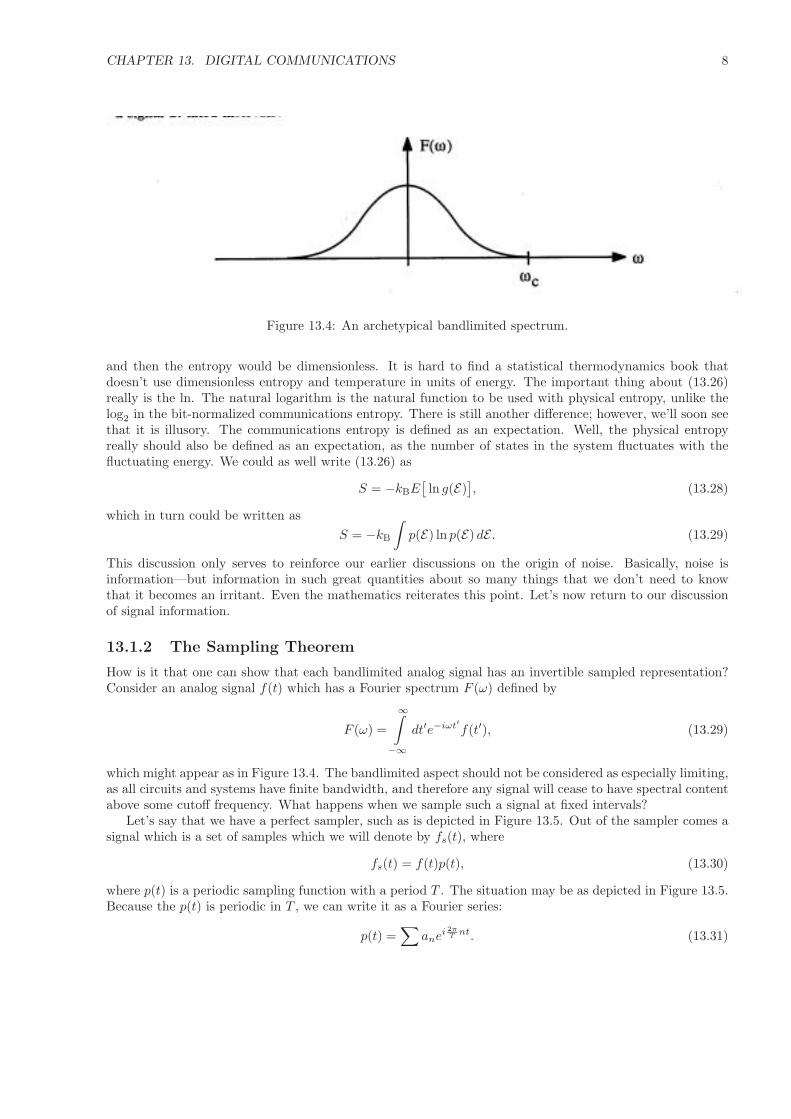
The two most interesting cases to us (for optical communications) are the NRZ code–that used in SONETand SDH–and the Manchester code, which is used in some datacommunication systems. In the NRZ, allis as we derived saw above if we simply take τi = τp in the above. The resulting spectrum may well looklike that depicted in Figure 13.10. The idea is that each sine function will have a zero at ±1/τi. The firstsinc function, sinc fτi, has its first zero there, so the first zero of the spectrum must fall at 1/τi. As all ofthe other sinc function in the expansion of (13.50) are narrower than the first one, one would expect thespectrum to be narrower than that of the first sinc taken alone. We really needn’t interest ourselves muchwith the spectrum beyond the first zero, as the receiver filter in general has a cutoff at this first zero point. AManchester code is one in which there are two symbols, both with 50% duty cycle but one with the pulse inthe first half of the τi frame and the other with the pulse in the last half. This isn’t quite in the form of thecase we calculated above, but from the calculation above we can draw some conclusions about a Manchestercode with the same τi as an NRZ. As the Manchester has a τp that is half that of the NRZ, the first zeroes ofthe spectrum will be at 2/τi, twice the frequency of the first zero of the NRZ. The Manchester spectrum willhave appreciable power at 1/τi. In the next section, we will see that this has implications for clock recovery.
13.2 The System Blocks in a Digital Optical Communications Sys-tem
A schematic block diagram of a digital optical communications system may appear as depicted in Figure 13.11below. Many of the pieces are the same as they were for the analog system of the last chapter. There aresome notable exceptions, however. The encoder and decoder will be quite different here, as digital coding isnothing like any coding would be in analog. The other major difference will be behind the amplifier—thatis, the filter, clock recovery, and decision circuitry.
It should be pointed out here that, although there can be many different kinds of digital optical systemsfor a multitude of operations, there are two types that stand out. Telephone systems have a definite set ofrequirements as well as the need for worldwide standardization. There are now a set of standards coveringthe transmission medium (physical level) of the telephone. The standards are collectively referred to as thesynchronous optical network (SONET) in the United States and as synchronous digital hierarchy (SDH) in
CHAPTER 13. DIGITAL COMMUNICATIONS 14
Figure 13.10: Sketch of a possible spectrum of a random bit stream compared to the spectrum of a singlepulse.
the rest of the world. Optical telephone systems at this point tend to consist of single-mode fiber, employlaser sources and PIN detectors, and operate at 1.3µm or 1.55µm. The long-haul part of the net (link lengthgreater than 80 km) generally employ erbium-doped fiber amplifiers (EDFAs), can use wavelength-divisionmultiplexing, and need to operate around 1.55µm in order to use the EDFAs. Another set of problemsis encountered in data communications where the distances may be much shorter than the point-to-pointdistances of telephone systems, but many require networking—that is, multiple tap points. Standards forsuch systems are beginning to converge. SONET basically fixes a number of standard rates (OC1 at roughly50 Mbs, OC3 at 150 Mbs, OC12 at 625 Mbs, OC48 at 2.5 Gbs, OC192 at 10 Gbs, OC768 at 40 Gbs, etc.)and then specifies the signal structure. All of these rates are based on the basic unit of one telephone callbeing 64 Kbs or the unit of DS1 of 24 telephone conversation or 1.5 Mbs. There is a 10-Mbs electrical localarea network (LAN) standard called ethernet. There is a fiber ethernet standard as well. There is anotherstandard called fiber distributed data interface (FDDI) which operates at 100 Mbs. There is presently workgoing on for 1-Gbs LANs and MANs (metropolitan area networks), called gigabit ethernet or GBE. Tothe present, most fiber LANs have employed multimode fiber (this may change in the future, at least forlonger distances at the higher bit rates), have used either LEDs or laser diodes at 1.3µm (although there ispresently a movement to go back operation at 0.83µm due to receiver cost), and generally use PIN diodes inthe receiver. As we go through the system blocks, we’ll see that there are differences between these systemtypes.
13.2.1 Digital Coding
As was touched upon in the last section, there are a number of ways to send quantized information. Wediscussed N -level pulse code modulation as a first example. In microwave communications, such codes with2N levels are generally used with phase shift keying and heterodyne detection. As will be discussed in thenext chapter, coherent optical receivers have not come so far as to do N -level detection. Essentially all digitaloptical communications is done with binary codes. It would be somewhat hard to imagine how one couldhave an N > 2 code for direct detection, as the system would not be especially robust and it might well besusceptible to non-graceful degradation with aging. In what follows, we’ll concentrate on binary codes.
Line codes basically come in two different types, the non-return to zero (NRZ) and the return to zero(RZ). Block codes really correspond to methods of including parity bits along with the information bits. Forexample, a block code of length 8 could include seven directly encoded bits plus a parity bit, which might beas simple as a modulo 2 sum of the proceding seven bits. This sum could be recalculated at the receiver to seeif the value received still agreed with the value calculated from the seven received bits. If not, clearly an errorhas occurred. There are also block codes such as pulse position modulation in which only one bit is on per

CHAPTER 13. DIGITAL COMMUNICATIONS 15
Figure 13.11: Schematic depiction of the pieces of a digital optical communications system.
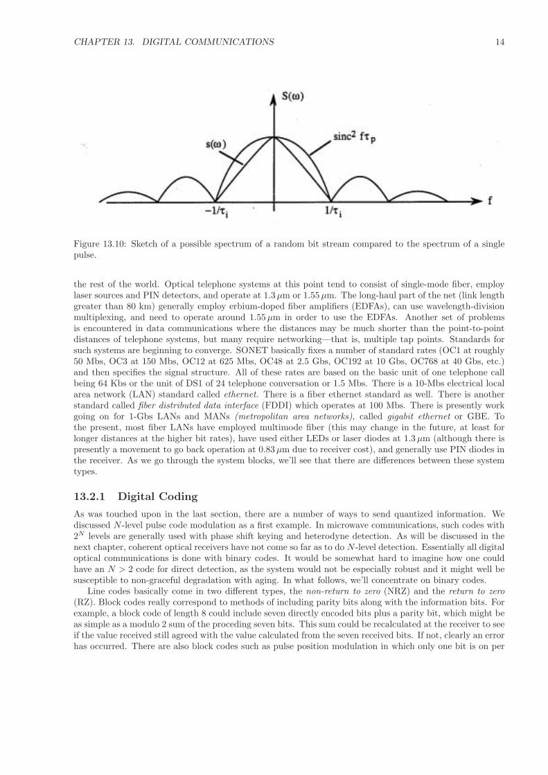
block. If the block is N bits long, then any of N words may be sent with a single bit, leading to a low powerrequirement, albeit a small effective transmission rate. For the present, we’ll consider only line codes as aresummarized in Figure 13.12 below, which is paraphrased from Keiser (1992). As can be perused from thediagram, the simplest, lowest bandwidth, highest signal-to-noise ratio code is the non-return to zero (NRZ),but it has two definite drawbacks. One is that it does not contain the fundamental frequency required forclock reconstruction except as a harmonic. As one does not want to have to tap too much power from thesignal, one wants the clock frequency signal (beat note) to be as strong as possible in the information streamto be sampled. There can therefore be a cost associated with not having the clock reconstruction note as thefundamental, as this may require one to draw more current from the signal in order to get enough power atthe beat note in order to lock the phase-locked loop. Both the unipolar and biphase have their fundamentalat the clock frequency, although the unipolar can exhibit fading. That is, the uniphase, given a long enoughset of transmitted zeroes, might lose clock synchronization. The biphase will always have a component atthe clock frequency, even during a long sequence of zeroes, as the biphase will still be changing state at theclock frequency.
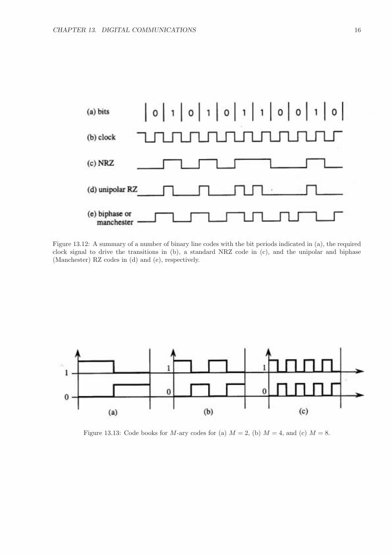
A major problem with SONET systems is that the ones that carry the highest bit rates are strapped forbandwidth. Forty-Gbs electronics doesn’t yet exist. As soon as 10-Gbs electronics existed, though, 10-GbsSONET systems followed. Telephone companies would always rather pack more data into the present cableplant than have to install a new cable plant. For this reason among others, SONET systems use NRZ code.A NRZ code only needs half the bandwidth of a Manchester code. LANs and MANs are only now reaching1 Gbs, a factor of ten below the OC192 SONET systems. As we will soon see, there are advantages toManchester code. The Manchester code is the M = 1 member of a set of orthogonal M -ary codes. TheM = 2, M = 4, and M = 8 code words are depicted in Figure 13.13. It can be shown (Schwartz 1970) thatthe M -ary codes are the optimal codes and can, in the limit M → ∞, even provide error-free transmission.The idea is that each symbol carries the same power and can be detected by filters matched to the pulseshapes. This of course assumes that there are no timing errors. However, as we saw in the last section, thereis a strong frequency component at the clock frequency, and, as we’ll soon see, this eases the problem ofclock recovery somewhat. In a LAN or MAN where a factor of two in bandwidth is available, the increasedreceiver sensitivity (that is, smaller power requirement for a given bit error rate due to the use of an optimalcode) and the simpler clock recovery circuit are worth the extra bandwidth requirement.
CHAPTER 13. DIGITAL COMMUNICATIONS 16
Figure 13.12: A summary of a number of binary line codes with the bit periods indicated in (a), the requiredclock signal to drive the transitions in (b), a standard NRZ code in (c), and the unipolar and biphase(Manchester) RZ codes in (d) and (e), respectively.
Figure 13.13: Code books for M -ary codes for (a) M = 2, (b) M = 4, and (c) M = 8.

CHAPTER 13. DIGITAL COMMUNICATIONS 17
13.2.2 Sources and Modulators
In SONET systems, the sources are generally lasers fabricated from quaternary materials such as InGaAsP.Generally, one also needs these lasers to be single-mode for both fiber coupling and to achieve the mini-mum dispersion penalty. Semiconductor lasers in quaternaries (unlike in GaAlAs/GaAs systems for “firstwindow”—0.78µm–0.85µm) don’t automatically achieve single-mode operation when properly index guided.For this reason, it is necessary to use distributed feedback (DFB) structures with these lasers to force single-mode operation. DFB lasers do not respond especially well to modulation, especially modulation at ratesgreater than 1 Gbs, and therefore SONET systems are using external modulators at the higher rates. ForOC48 (2.5 Gbs), most systems use electroabsorption modulators which can be monolithically integrated withthe laser structure. At higher rates, it may be necessary to go over to LiNbO3 modulators, which seem tohave no real speed limitations.
For multimode networking systems, both lasers and LEDs are employed. Lasers for such operation mustbe either multimode or “dithered” to enhance their linewidths to reduce any modal noise penalty. For a62.5-µm, 0.26-NA multimode fiber, one generally needs to have a source linewidth of greater than roughly0.5 nm to eliminate the modal noise penalty. Interestingly enough, this linewidth is essentially the linewidthfor which the fiber modes become a continuum, as was discussed in Chapter 10. There are no “practical”multimode modulators such as there are for single-mode systems. For this reason, multimode systems usedirect laser modulation. As was discussed in the last chapter, the laser or LED therefore becomes a circuitelement in the transmitter. As we saw in the last chapter, a laser appears to the circuit as a resonatingelement. This resonance, known as the relaxation oscillation peak, generally lies above roughly 3 GHz fortypical 300µm-long cavities in either the ternary or quaternary materials. Modulation depth is enhanced atthe resonance and greatly diminished above it (the 20-dB/decode rolloff of a two-pole filter). This peak is,therefore, roughly the limiting factor for modulation bandwidth in LAN-type systems.
It should be pointed out that the distinction between SONET, SDH, and networking systems may becomeeven more blurred in the future. The internet is one of the causes of this. Back in the 1950s, the DefenseAdvanced Projects Administration (DARPA) decided to launch a program where existing communicationnetworks could be used even if major sections of the network were knocked out by a nuclear attack and theelectromagnetic pulse that would accompany it were the weapons to be used “optimally”—that is, explodeda bit above the surface of the land being attacked. The way to optimize the communications system was touse packet switching rather than circuit switching. In circuit switching, once the path is set up it remainsfixed until the message is over. With packet switching, as the message is being sent and after each fixedlength of information, it is sent off with a header. The packet then finds any route that is open to get to itsdestination. At the destination, software is used to reconstruct the message. Packet switching, or variationsthereof, are the rule for networking systems. At this point in time, however, telecos as well as cable companiesand independent entities would like to send telephone, CATV, internet access, and whatever else over thesame set of lines. Switches and systems which can handle both SONET and network information are everappearing. As such systems must handle the high-speed SONET, they appear as SONET systems. Theexpense of such systems, though, will preclude such applications as workstation networks for the foreseeablefuture.
13.2.3 Filtering at the Linear Amplifier Output
In Chapter 10, discussion of both multimode and single-mode channels was given in some detail. Detectors,both PIN and APD (in the last chapter) have been discussed along with receiver front ends and linear ampli-fiers in the last chapter. Discussion, then, will presently turn to the filtering performed after amplification.
The basic reason for having a filter at the output of the linear amplifier is that the circuit noise, shot noise,and any spontaneous emission noise has a virtually flat spectrum, whereas we saw in the last section that thespectrum of a binary signal can be bandlimited without losing information. Signal-to-noise ratio can thenbe improved significantly at the amplifier. Certainly, the detector/preamplifier circuit is also bandlimitedand, to manage costs, bandlimited to a limit which shouldn’t too greatly exceed the limit of the signal.However, the design of the front end is really more concerned with passing as much signal as possible. Thefilter section is concerned with blocking noise without attenuating signal. In the last chapter, we discussedoptimal filtering—that is, the Wiener filter which can be applied to an arbitrary signal spectral profile. With

CHAPTER 13. DIGITAL COMMUNICATIONS 18
a binary switched signal, the main feature we recognize about the signal—i.e. the cutoff point—and that atbest it will be a bit narrower than the diode width corresponding to a single pulse. For this reason, one mayas well use a standard filter solution for a lowpass filter where essentially the only parameter specified is thecutoff.
An ideal lowpass filter would have the transmission function T (f) given by
T (f) = rect(
f
fc
)(13.51)
—that is, would have a sharp cutoff. Unfortunately, the Fourier transform of T (f), T (t), is given by
T (t) = fc sinc(fct). (13.52)
The effect of a filter on a signal s(t) with transform S(f) is to generate sf (t) and Sf (f), where
sf (t) = T (t) ∗ s(t) (13.53a)
Sf (f) = T (f)S(f). (13.53b)
The frequency domain response is the one that we want, but the time domain response is a bit problematic.If we were to say that s(t) is zero for t ≤ 0, we would still have a filtered version sf (t) that starts at −∞.The frequency response—that is, the filter is outputting a filtered signal before the signal arrives at the filter.Circuits, we know, have causal outputs, and further, circuit transfer functions must be of the form
T (s) =ZT∏i=1
(s − szi)
PT∏i=1
1s − spi
, (13.54)
where ZT < PT . For a stable circuit, we further would have that
spi< 0 ∀ pi. (13.55)
The frequency response of such a filter would be given by evaluating the T (s) for s = jω. We with to lookat the class of filters for which ZT = 0—that is, the class of all pole filters for which
T (ω) = (−j)PT
PT∏i=1
1ω − ωpi
. (13.56)
Such filters have more linear phase characteristics than ones with finite zeroes (Moschytz and Horm 1981).Nonlinear phase characteristics lead to pulse dispersion.
A frequency response such as (13.56) corresponds to an inverse polynomial. As we all well know, thereare any number of orthogonal polynomials. Essentially any set of orthogonal polynomials will lead to a set offilters where the order of the polynomial gives the order of the filter. Indeed, there are Legendre, Chebyshev,and Bessel filters. Chebyshev filters have a very sharp cutoff but exhibit ripple in the passband. Bessel filtershave not nearly so sharp a cutoff as a Chebyshev filter but have a very nearly linear phase response so thatpulses output from the filter show little or no ringing or overshoot. Another filter known as a Butterworthfilter is not quite so phase-linear as a Bessel filter but has an essentially flat amplitude response in its passbandand a much sharper cutoff response than a Bessel filter. Generally, Bessel or Butterworth filters are employedas the filters of choice in digital systems. More discussion of filtering, including techniques to find activefilter implementations, is given in Moschytz and Horn (1981). As was discussed in Chapter 4, active filterimplementations are advantageous in that some amount of gain can be combined with the spectral shapingoperation. As receiver front ends generally employ transimpedance amplifiers which need an amplifier thatfunctions as a operational amplifier, the filtering operation can employ a similar technology, and this leavesopen the possibility of monolithic receiver integration.

CHAPTER 13. DIGITAL COMMUNICATIONS 19
Figure 13.14: A possible clock recovery circuit in which the signal is bandpass filtered to obtain a sine wavewhich is phase-locked looped before being injected into a comb generator and then an integrator to generatea square pulse train which can then be input to the filter and decision circuitry.
13.2.4 Clock Recovery and Timing Errors
In a digital system, there is always the question of whether the system should be run synchronously orasynchronously. In a standard computer system, one in general has a clock distribution so that each gate isrunning to the same time synch. Even though the standard for the physical level of the telephone networkis called SONET for synchronous optical network, this name is a bit confusing for a couple of reasons. Oneis that the higher logical levels of the IEEE 488 standard that is inevitably used to insert and receive datafrom SONET can actually support such protocols as ATM (or asynchronous transfer mode). The other isthat, with transmission over a long distance with random connection path, one cannot distribute a clockto everywhere independent of the transmission path, but instead the receivers need to somehow reconstructthe timing information from the signal. The “synchronous” in SONET really refers to the fact that the datarates, bit shapes, and parity bit placements in the stream are all standardized at each level in the networksuch that everybody can use the same transmission and reception equipment and does not mean synchronousin the computer sense that there is only clock distribution to everywhere in the system.
The circuit that performs the timing information reconstruction is generally called the clock recoverycircuit. A possible realization of a clock recovery circuit is shown in Figure 13.14. The circuit is actuallya bit more general than need be. The signal has already been through a lowpass filter. The phase-lockedloop really functions as a narrow bandpass filter. Generally, clock recovery implementations employ eithera phase-locked loop or a narrowband bandpass filter—not both. In SONET, the information rates are quiteconstrained. For example, OC48, which we have said before is a rate of 2.5 Gbs, is not totally accurate. Itis actually 2.488 Gbs. The SONET rates are constrained to four significant figures or to about 1 MHz infrequency space. A filter has a fixed passband, so information rate drift can knock out a system. This is notmuch of a problem with SONET. With packet switching, it can be, as a few bits of header must be sufficientto synchronize the receiver. A phase-locked loop here is necessary, if not a combined phase and frequencylock if drift is significant. (See, for example, Pottbacker et al 1992.) Some research is currently going intoall-optical clock recovery techniques as well, as indicated by recent literature (Wang et al 1998, Dulter et al1995, Kawanishi et al 1993). Other high-speed techniques are also being proposed (Fang et al 1995, Imai etal 1993). In what follows, we will discuss a filtering technique and a phase-locked loop technique.
We included some considerable discussion of electrical filtering in section 4.6 of Chapter 4. We showedthat, if we had a bandpass filter with 2Np poles—Np on the low-frequency side and Np on the high-frequencyside—the rejection at the next sideband would be 1
2Np, 13Np at the third sideband, etc. For a sharp-edged
digital pulse, there can be many sidebands, each of them nearly as strong as the fundamental. To get goodrejection (20–30 dB) would require an inordinate number of filtering stages, each contributing some loss

CHAPTER 13. DIGITAL COMMUNICATIONS 20
to an already weak signal. An alternative solution which is coming more and more into use is the surfaceacoustic wave (SAW) filter, which we will presently discuss.
Surface acoustic wave (SAW) devices are interesting in their own right. The basic idea behind theseelectric filtering devices could be described as follows. A material which is unstressed will also be unstrainedin the sense that the equilibrium positions of all of the material elements which we will define by a functionu(x, y, z) will be in their unstressed positions u0(x, y, z) such that
∂uj
∂xi+
∂ui
∂xj= 0, (13.57)
wherex1 = x (13.58a)
x2 = y (13.58b)
x3 = z. (13.58c)
Any stress applied to the material will cause the elements of the strain tensor Sij , defined by
Sij =12
(∂uj
∂xi+
∂ui
∂xj
), (13.59)
to become nonzero. The (lowest-order linear) relation between the stress tensor Tij and the strain tensorSk is given by Hooke’s law in terms of the constitutive tensor Cijk by
Tij =∑k
CijkSk, (13.60)
where the elements of the stress tensor denote the force per unit area applied to an ordered element of area.The on-diagonal elements Tii, therefore, denote compressional forces, and the off-diagonals Tij , where i = j,are shears. Newton’s law tells us that force must be mass times acceleration. The force density, though,must be dimensionally given by ∑
j
∂Tij
∂xj= fi, (13.61)
where fi is the force density, which in turn must be given by
fi = ρ∂2ui
∂t2, (13.62)
where ρ is the material mass density. Combining Hooke’s law with the divergence of Tij with the force lawgives us
ρ∂2ui
∂t2=∑jk
∂
∂xjCijk
(∂uj
∂xi+
∂ui
∂xj
), (13.63)
which is a second-order wave equation and shows that we can have phonon propagation in crystalline-typemedia. This still isn’t too useful, though.
Certain materials exhibit a so-called piezoelectric effect in which there is a coupling between polarizability(electric) and stress/strain (mechanical). This electromechanical coupling leads to a modification of Hooke’slaw to the form
Tij =∑k
CEijkSk −
∑k
eijkEk (13.64a)
Di =∑k
εikSk +∑
k
εSikEk, (13.64b)
where eijk is the piezoelectric tensor, E is the electric field vector, D is the electrical displacement vector, εSij
is the electrical permittivity tensor when a strain tensor S is present, and CEijk is the mechanical constitutive
tensor in the presence of an electrical field. The important thing to note from the above is that the electric
CHAPTER 13. DIGITAL COMMUNICATIONS 21
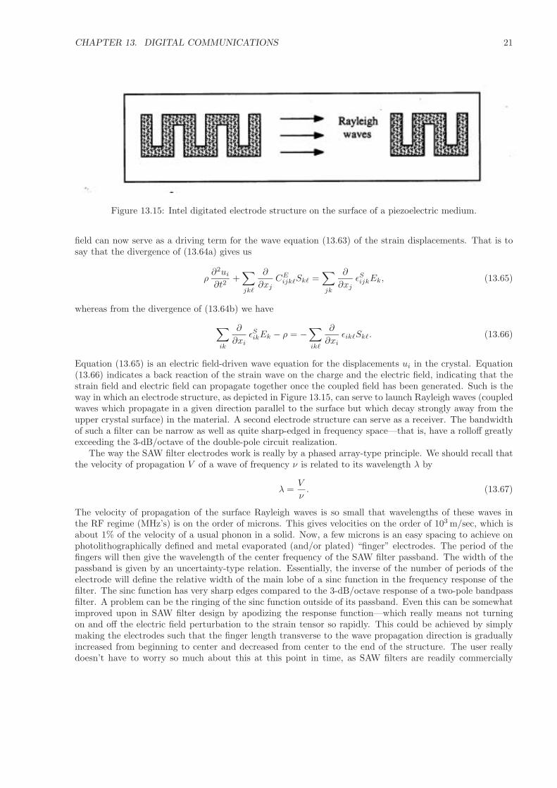
Figure 13.15: Intel digitated electrode structure on the surface of a piezoelectric medium.
field can now serve as a driving term for the wave equation (13.63) of the strain displacements. That is tosay that the divergence of (13.64a) gives us
ρ∂2ui
∂t2+∑jk
∂
∂xjCE
ijkSk =∑jk
∂
∂xjεSijkEk, (13.65)
whereas from the divergence of (13.64b) we have∑ik
∂
∂xiεSikEk − ρ = −
∑ik
∂
∂xiεikSk. (13.66)
Equation (13.65) is an electric field-driven wave equation for the displacements ui in the crystal. Equation(13.66) indicates a back reaction of the strain wave on the charge and the electric field, indicating that thestrain field and electric field can propagate together once the coupled field has been generated. Such is theway in which an electrode structure, as depicted in Figure 13.15, can serve to launch Rayleigh waves (coupledwaves which propagate in a given direction parallel to the surface but which decay strongly away from theupper crystal surface) in the material. A second electrode structure can serve as a receiver. The bandwidthof such a filter can be narrow as well as quite sharp-edged in frequency space—that is, have a rolloff greatlyexceeding the 3-dB/octave of the double-pole circuit realization.
The way the SAW filter electrodes work is really by a phased array-type principle. We should recall thatthe velocity of propagation V of a wave of frequency ν is related to its wavelength λ by
λ =V
ν. (13.67)
The velocity of propagation of the surface Rayleigh waves is so small that wavelengths of these waves inthe RF regime (MHz’s) is on the order of microns. This gives velocities on the order of 103 m/sec, which isabout 1% of the velocity of a usual phonon in a solid. Now, a few microns is an easy spacing to achieve onphotolithographically defined and metal evaporated (and/or plated) “finger” electrodes. The period of thefingers will then give the wavelength of the center frequency of the SAW filter passband. The width of thepassband is given by an uncertainty-type relation. Essentially, the inverse of the number of periods of theelectrode will define the relative width of the main lobe of a sinc function in the frequency response of thefilter. The sinc function has very sharp edges compared to the 3-dB/octave response of a two-pole bandpassfilter. A problem can be the ringing of the sinc function outside of its passband. Even this can be somewhatimproved upon in SAW filter design by apodizing the response function—which really means not turningon and off the electric field perturbation to the strain tensor so rapidly. This could be achieved by simplymaking the electrodes such that the finger length transverse to the wave propagation direction is graduallyincreased from beginning to center and decreased from center to the end of the structure. The user reallydoesn’t have to worry so much about this at this point in time, as SAW filters are readily commercially

CHAPTER 13. DIGITAL COMMUNICATIONS 22
available from a number of sources and are well specified by the product literature. This is in part drivenby the fact that SAWs are the filters of choice for digital television and will soon find broad application. Aproblem can be that most SAW materials exhibit a great increase in acoustic wave propagation attenuationabove circa 1 GHz. It seems that optical communication rates, at least for the telecos, will continue toincrease above the 1-Gbps rate for the foreseeable future.
After the SAW filter, there may not be too much signal left, although we would hope that what there iswould be quite clean. The width of the SAW peak in general could be made about as narrow as one couldwant and is generally specified with respect to being greater than the maximal drift that could be suffered bythe center frequency of the clock peak. As one wants to preserve the phase of this frequency component, anobvious way to amplify it is to inject it onto a phase-locked loop. The idea here really goes back to some ofthe discussion of Van der Pol oscillators in Chapter 4. One might recall that the equation for the dynamicalbehavior of an oscillating circuit was given by
∂2v
∂t2+ δ
(1 − v2
v0
) ∂v
∂t+ ω2
0v = Aω20ve(t), (13.68)
where the ve term on the right-hand side indicates an external term which can be injected into the oscillator.If A is small enough, this term will have little or no effect on the oscillation, and the solution to theVan der Pol equation will have the form
v(t) = v0 cos(ω0t + φ0). (13.69)
If the injected signal, then, is of the form
ve(t) = ve cos(ωet + φe) (13.70)
and if the amplitude ve and coupling strength A are large enough, the v(t) will lock to the signal—that is,v(t) will become a replica of ve(t) although maybe with much larger amplitude. There is a tradeoff, however,in that if the signal is below some threshold, the lock will not be complete. Infinite gain in the phase-lockedamplification, as would be expected, is not available.
A straight filtering technique such as that described above would be fine for a Manchester code, wherethe incoming signal would have a strong component at the clock frequency. For a NRZ code, though, anadded element would be necessary. That element could be as simple as a half-wave rectifier (diode) at theinput of an amplifier to boost the signal level.
Other techniques we want to discuss in combination with clock recovery is the technique which uses aphase-locked loop. There are various configurations which can be employed. For an NRZ code, we may wellwant to employ such a circuit as schematically depicted in Figure 13.16. The NRZ signal is input to thephase-locked loop. The signal is then mixed with the output signal of a voltage-controlled oscillator whichis tuned to be close to what the clock frequency should be. (The oscillator cannot drift anywhere near asfar as half the frequency of the clock due to a limited loop bandwidth.) The loop filter in this phase-lockedloop is then just simply an integrator. The idea behind this is illustrated in Figure 13.17, which shows thatthe error signal will “null” when the clock locks in phase and frequency to the NRZ signal incident. If theclock is not in lock, the error signal will steer the oscillation toward lock. The locked clock signal is thenused to gate on (on the raising edge) an integrator which then puts out a flat level each clock period whichcan be thresholded to decide whether it is a zero or a one in the information stream.
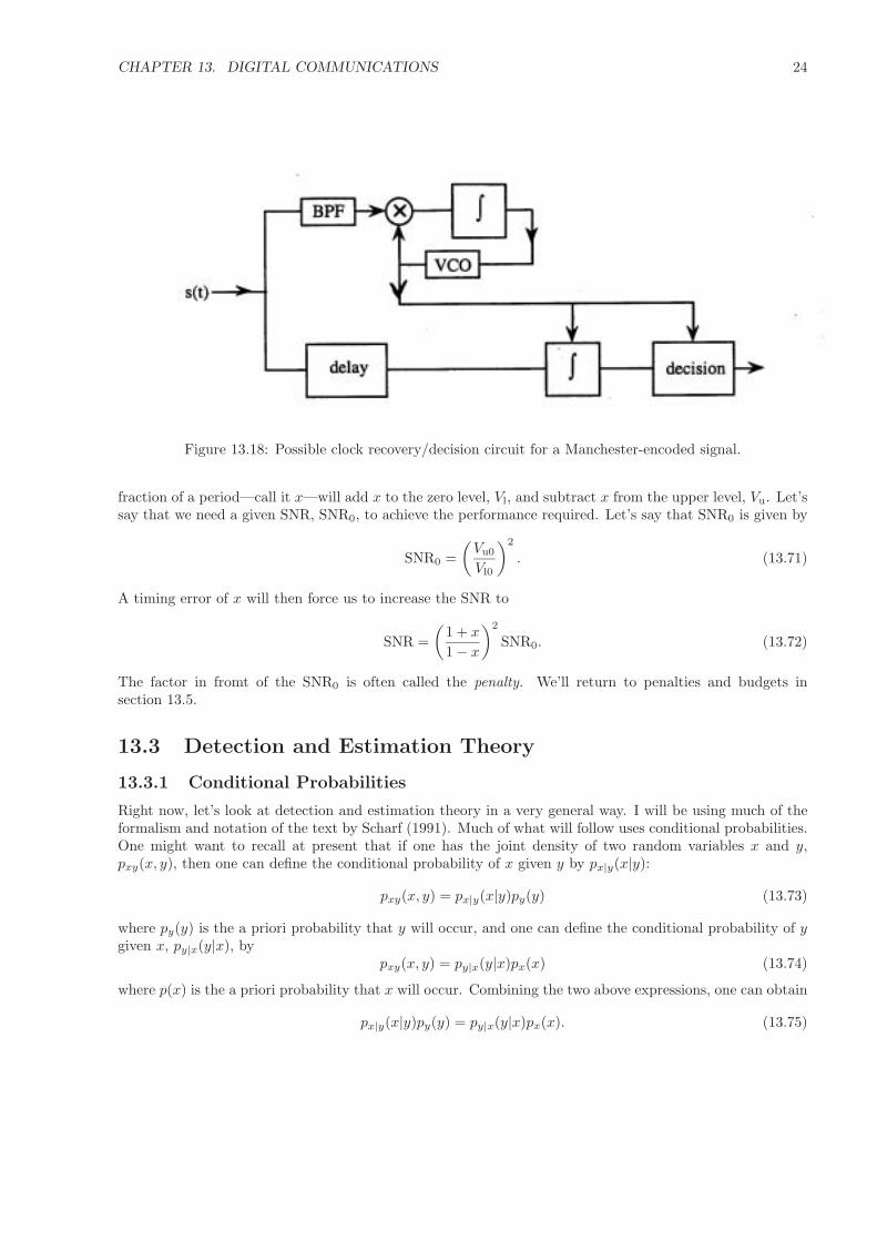
A clock recovery/decision circuit for a Manchester-coded signal may appear as in Figure 13.18. Hereone bandpasses the signal before inputting it to the phase lock. Here the filtered signal is multiplied by theoutput of a VCO which is tuned close to the clock frequency—that is, close to the frequency of the signalbeing input to the loop. One can readily convince oneself that, if the VCO is tuned to the clock frequencybut 90 out of phase, the error signal will go to zero and lock will be obtained. The decision is then madeby checking if the voltage out of the gated integrator is positive or negative.
Clock recovery is important from the standpoint of intersymbol interference (ISI). Pulses are not com-pletely square, due to both dispersion and the filter at the output of the linear amplifier. This means thata zero level is not zero even in the absence of circuit noise and dark current. The worst case would be fora zero between two ones. Timing errors can greatly exacerbate this situation, as an error of, for example, a

CHAPTER 13. DIGITAL COMMUNICATIONS 23
Figure 13.16: An archetypical clock recovery and decision circuit for a NRZ coded signal.
Figure 13.17: A timing diagram showing how the loop error signal will null when the clock has the rightphase and frequency relative to an NRZ signal.
CHAPTER 13. DIGITAL COMMUNICATIONS 24
Figure 13.18: Possible clock recovery/decision circuit for a Manchester-encoded signal.
fraction of a period—call it x—will add x to the zero level, Vl, and subtract x from the upper level, Vu. Let’ssay that we need a given SNR, SNR0, to achieve the performance required. Let’s say that SNR0 is given by
SNR0 =(
Vu0
Vl0
)2
. (13.71)
A timing error of x will then force us to increase the SNR to
SNR =(
1 + x
1 − x
)2
SNR0. (13.72)
The factor in fromt of the SNR0 is often called the penalty. We’ll return to penalties and budgets insection 13.5.
13.3 Detection and Estimation Theory
13.3.1 Conditional Probabilities
Right now, let’s look at detection and estimation theory in a very general way. I will be using much of theformalism and notation of the text by Scharf (1991). Much of what will follow uses conditional probabilities.One might want to recall at present that if one has the joint density of two random variables x and y,pxy(x, y), then one can define the conditional probability of x given y by px|y(x|y):
pxy(x, y) = px|y(x|y)py(y) (13.73)
where py(y) is the a priori probability that y will occur, and one can define the conditional probability of ygiven x, py|x(y|x), by
pxy(x, y) = py|x(y|x)px(x) (13.74)
where p(x) is the a priori probability that x will occur. Combining the two above expressions, one can obtain
px|y(x|y)py(y) = py|x(y|x)px(x). (13.75)

CHAPTER 13. DIGITAL COMMUNICATIONS 25
If, for example, px(x) is the a priori probability that we transmit a one and py(y) is the a priori probabilitythat we receive a one, then if we knew something about our channel and we could compute the a prioriprobability that we had received a one given that was what we transmitted, we could compute the a posterioriprobability that a one was sent given that we have already received a one by
px|y(x|y) =px|y(y|x)px(x)
py(y), (13.76)
which is a form of the so-called Bayes rule. We will see this relation again in what follows. Two useful thingsto recall about conditional probabilities which follow from the relations∫
p(x, y) dx = p(y);∫
p(x, y) dy = p(x) (13.77)
and ∫p(x) dx = 1;
∫p(y) dy = 1 (13.78)
are that the normalizations of the conditional probabilites are∫p(x|y) dx = 1 (13.79)
and ∫p(y|x) dy = 1. (13.80)
Let’s first consider the more general case of the estimation of a continuous parameter from a measuredvalue and later specialize to cases where we need only decide between a discrete number of hypotheses—i.e. the digital case. In the following, we will carry out the bit error rate (BER) calculations in terms ofthe pdf’s of the receiver current. This probably requires some comment, as in the previous section wediscussed in some detail how a decision is made on a voltage. As it turns out, the situation in the receiver issimilar to that in the channel. For example, in a system with a laser radiating into a fiber whose output inturn illuminates a detector, there are two ways to make the calculation of the pdf conditioning the currentgeneration. One would be to first find the pdf of the source, then propagate this pdf (or density matrix,if you will) through the system using difference equations as in Chapter 10, through to a detector surface.Because of the nature of the conditional process, however, one could equivalently propagate a classical fieldfrom the laser through the fiber and convert the classical field to a pdf at the detector. Even for a systemwith optical amplifiers, we could propagate classical fields through the system so long as we propagated twoof them, a deterministic one and a random one, to be combined into a discrete pdf at the detector using theRician density and conditional Poisson statistics. In a major sense, a similar thing is true in the receiver.In the preamplifier circuit, noise is added to the current, and one can find a pdf for this current. At theoutput of the preamplifier, there is a voltage—but one that has been amplified sufficiently that its level ishigh above any circuit noise level. Classical circuit theory can then be applied to amplification and filteringso long as one takes the amplifier noise figure in computing the circuit noise—that is, the noise temperaturewill be above room temperature. One can then assume an ideal decision circuit and worry about the effectsof timing errors along with channel effects such as dispersion as being contributors to ISI, which is includedafter the BER calculation and included as a penalty (to be discussed further in the next section). Thepropagation of the current to the decision circuit can then be simply considered as an overall amplificationnoise and a filtering. These two factors are straightforward to put into the pdf that was calculated for thecurrent at the input to the preamplifier. The noise figure will add Gaussian noise to the filter bandwidth,and our conditioning numbers for the statistical modes of any amplitude-spontaneous emission (ASE) needto be calculated using the filter bandwidth.
Let’s say, without any real loss of generality, that we want to determine the best estimate m of a countparameter m from the measurement i of a current i. The first thing that needs to be done is to define aso-called loss function (m, m) which defines what it is we would like to minimize. This is often taken to bethe mean-squared error such that
(m, m(i)
)=(m − m(i)
)2, (13.81)

CHAPTER 13. DIGITAL COMMUNICATIONS 26
where we have explicitly noted the dependence m of the measurement on i. We then define a risk functionR(m, m) such that
R(m, m(i)
)= Eim
[ (m, m(i)
)]. (13.82)
That is, the risk function is the expectation value of the loss function averaged over the joint distributionthat we receive a current i and that the condition number m was sent, pim(i,m). We would write thisexpectation in the form
R(m, m(i)
)=∫
(m, m(i)
)pim(i,m) di. (13.83)
13.3.2 Bayes Estimation
In Bayes estimation, we assume that we know the a priori distribution of m, pm(m), which gives theprobability that we will send a given level m. We can then write a new risk function R
(pm(m), m
)as a
function of this a priori density in the form of an expectation of the risk function R(m, m(i)
):
R(pm(m), m(i)
)= Em
(R(m, m(i)
)), (13.84)
which can be written out as
R(pm(m), m(i)
)=∫
R(m, m(i)
)pm(m) dm (13.85)
or, by back-substituting,
R(pm(m), m(i)
)=∫ ∫
(m, m(i)
)pim(i,m) di dm. (13.86)
We can express the joint density, though, as a function of the a posteriori probability pm|i(m|i) and thea priori probability pi(i) by
pim(i,m) = pm|i(m|i)pi(i) (13.87)
to findR(pm(m), m(i)
)=∫ ∫
(m, m(i)
)pm|i(m|i) dmpi(i) di. (13.88)
With this, we see that we can express the Bayes estimator mB as
mB = minm
∫ (m, m(i)
)pm|i(m|i) dm, (13.89)
where we have removed the p(i) di, without loss of generality, as it will not affect the value mB in theminimization. (If you wish, leave it in the expressed (13.89) and go through the derivation of (13.97) tonotice that the inclusion of p(i) di has no effect on the Bayesian estimator mB.) Let’s say that we take ourloss function to be squared error. Then we can re-express mB in the form
mB = minm
∫(m − m)2pm|i(m|i) dm. (13.90)
To minimize, we need to take a derivative and set the whole expression equal to zero:
∂
∂m
∫(m − m)2pm|i(m|i) dm = 0. (13.91)
Using the fact that ∫pm|i(m|i) dm = 1, (13.92)
we find thatmB =
∫mpm|i(m|i) dm, (13.93)

CHAPTER 13. DIGITAL COMMUNICATIONS 27
which is just the expectation of the a posteriori probability pm|i(m|i) by
mB = Em
(pm|i(m|i)). (13.94)
However, we don’t have pm|i(m|i), but we can use Bayes’ rule to write
pm|i(m|i) =pi|m(i|m)pm(m)
pi(i)(13.95)
and to write
mB(i) = Em
[pi|m(i|m)pm(m)pi(i)
], (13.96)
which is also expressible as
mB(i) = Em
[pim(i,m)pi(i)
]. (13.97)
For an example, let’s say that our signal is completely deterministic but that the current noise is Gaussiansuch that
pim(i,m) =1√2πi2n
exp− (i − mi0)2
2i2n
(13.98)
and any current is equally likely to occur, allowing us to ignore the factor pi(i) which is independent of i.With this, we can write that
pm|i(m|i) =1√2πi2n
exp− (i − mi0)2
2i2n
. (13.99)
The mean of this distribution with respect to m is just
mB =i
i0, (13.100)
more or less what one would have expected.Before going on to the other technique of estimation, namely that one which employs the principle of
maximum likelihood, let’s consider applying Bayesian estimation to a problem in digital detection. In sucha case, our m can take on only two values such that we can write that
pm(m) =
p0, m = m(0)
p1, m = m(1).(13.101)
This tells us that the distribution for the current can be expressed as
pi(i) = p0pi|m(0)
(i|m(0)
)+ p1pi|m(1)
(i|m(1)
). (13.102)
Our problem amounts to having to decide from a received current value i whether the character that wastransmitted was a one or a zero. If we say that what we are doing is hypothesis testing, we would say thatthere are two hypotheses H0 and H1, each corresponding to a possible transmission. We are trying to definea decision rule ϕ(i) such that
ϕ(i) =
1 (H1), i ⊃ S1
0 (H0), i ⊃ S0.(13.103)
That is, we are trying to section our possible result space of receivable currents into two sets S0 and S1, andif we receive a current in set S1 we will decide that our hypothesis H1 is correct. If we receive a currentin S0, we will decide on H0. If the sets S0 and S1 are not disjoint, essentially what we are trying to do is
CHAPTER 13. DIGITAL COMMUNICATIONS 28
decide on a threshold current ith such that when i < ith we assume that a zero was sent and when i > ithwe assume that a one was sent.
We now need to design a Bayes test. To do this, we’ll need to define a loss function and a risk functionand then do an optimization. Our loss function in this case is simply a set of four for values which we canexpress in a matrix component form:
(m(j), ϕ(i)
)= jk (13.104)
where j = 0, 1 and k = 0, 1. Our risk function becomes
R(m(j), ϕ(i)
)= Em
[ (m(j), ϕ(i)
)], (13.105)
which can be written out termwise as
R(m(j), ϕ(i)
)=
00p(ϕ(i) = 0|m(1)
)+ 01p
(ϕ(i) = 1|m(0)
), m = m(0)
10p(ϕ(i) = 0|m(1)
)+ 11p
(ϕ(i) = 1|m(1)
), m = m(0).
(13.106)
We can simplify the notation by writing
p(ϕ(i) = 0|m(0)
)= 1 − α (13.107a)
p(ϕ(i) = 1|m(0)
)= α (13.107b)
p(ϕ(i) = 0|m(1)
)= 1 − β (13.107c)
p(ϕ(i) = 1|m(1)
)= β, (13.107d)
where α is often referred to as the probability of false alarm, β as the probability of detection, and 1 − βas the probability of a miss. This terminology comes from radar where, from a received signal, one has todecide if there was something there or not. We can then rewrite the risk function in the form
R(m(j), ϕ(i)
)=
( 01 − 00)α + 00, m = m(0)
( 10 − 11)(1 − β) + 11, m = m(1).(13.108)
What is generally done at this point is to set
00 = 0; 11 = 0 (13.109)
and then write the Bayes risk in the form
R(pm(m), ϕ(i)
)= p0 01α + p1 10(1 − β), (13.110)
which we could rewrite in the form (assuming that neither S0 nor S1 have disjoint portions)
R(pm(m), ϕ(i)
)= p0 01
∞∫ith
pi|m(0)(i) di + p1 10
ith∫−∞
pi|m(1)(i) di, (13.111)
where the notation with the m(0) and m(1) missing in the arguments but not the subscripts should be clear,as with conditional probabilities the functional dependence is only on the variable—not on the given. Theoptimization can then be performed by
∂R(pm(m), ϕ(i)
)∂ith
= 0, (13.112)
which then gives us the expression
p1 10pi|m(1)(ith) = p0 01pi|m(0)(ith) (13.113)

CHAPTER 13. DIGITAL COMMUNICATIONS 29
Figure 13.19: Plots of the current distributions for zeroes and ones, where the cross-hatched region indicatesthe area in which errors must occur.
to define our threshold current, which in turn gives us our decision rule:
ϕ(i) =
1,pi|m(1) (i)
pi|m(0) (i)> p001
p110
0, otherwise,(13.114)
where the ratio of the densities is called the likelihood ratio and the probability and the loss function ratiois called the threshold. The test is called a likelihood ratio test. The situation is illustrated in Figure 13.19for the case where p0 01 = p1 10. The idea is that errors will occur in the regions where the distributionsoverlap. The total probability of error PE is given by
PE =
ith∫−∞
pi|m(1)(i) di +
∞∫ith
pi|m(0)(i) di, (13.115)
which is just the risk function evaluated with the optimized threshold. This probability of error, PE, is alsocalled the bit error rate (BER), allowing us to write that
BER = minith
R(m(j), φ(i)
). (13.116)
We’ll take a look at some BER calculation examples at the end of our upcoming discussion of maximumlikelihood estimation and detection under the Neyman-Pearson criterion.
13.3.3 Maximum Likelihood
A second method of doing estimation and detection theory is to simply use the maximum likelihood principle.The results of this theory are similar but not identical to those using Bayes’ theory in many of the simplercases such as for simple scalar detection and estimation. However, the Bayesian approach can be generalizedto treating sampled time series as a form of vector estimation and can therefore be used to derive suchuseful prediction schemes as Kalman filtering. As we’ll soon see in examples, though, there is a power andsimplicity to maximum likelihood which can be extended to time series as well.
The maximum likelihood principle is easily stated. It is simply that the maximum likelihood estimate ofm is the value m of the conditioning parameter m for which the observed current value i is most likely tohave occurred, which is to say that
m = maxm
p(i,m). (13.117)

CHAPTER 13. DIGITAL COMMUNICATIONS 30
So, given an observed value i of the current, we simply search the joint distribution p(i,m) for the m valuem which maximizes the probability. Generally, one defines a likelihood function L(m, i) as the logarithm ofthe joint density:
L(m, i) = ln p(i,m), (13.118)
and a score function as the derivative of this:
S(m, i) =∂
∂mL(m, i), (13.119)
and the Fisher determinant as the negative of the second derivative:
F (m, i) = − ∂2
∂m2L(m, i). (13.120)
With all of these definitions, we see that the maximum likelihood estimate is given as the solution of
S(m, i) = 0. (13.121)
Perhaps a couple of examples can illustrate the technique.Let’s consider a deterministic signal corrupted by Gaussian noise such that
p(i,m) =1√2πi2n
exp− (i − mi0)2
2i2n
. (13.122)
In this case, the loss function becomes
L(m, i) = − (i − mi0)2
2i2n− 1
2ln(2πi2n), (13.123)
and the score function isS(m, i) =
i0
i2n(i − mi0), (13.124)
which gives us the maximum likelihood estimator
m =i
i0(13.125)
and the Fisher determinant
F (m, i) = mi20
i2n, (13.126)
which just tells us that we have indeed found a maximum.Our second example will now show us how we can extend all of our earlier results to sampled data vectors
i and vectors of conditioning number m. Let’s say that we choose N independent, identically distributed(i.i.d.) values from a Gaussian distribution which is formally the same as the one we considered in the lastproblem. Let’s say that we want to estimate both the mean and the standard deviation of the distributionfrom our measurements, which then makes our conditioning vector m equal to
m =( i
i2n
)=(
m1
m2
). (13.127)
Our joint probability distribution of the measurements will then be
pim(i,m) =N−1∏j=0
e
(i−i)2
2i2n√2i i2n
, (13.128)

CHAPTER 13. DIGITAL COMMUNICATIONS 31
which can be rewritten in the form
pim(i,m) =
1√2πi2n
N
exp
− 12i2n
N−1∑j=0
(ij − i)2
. (13.129)
The loss function then becomes
L(m, i) = − 12i2n
N−1∑j=0
(ij − i)2 − N
2ln[2πi2n]. (13.130)
The score function becomes the vector function
S(m, i) =
−Ni
i2n+ 1
i2n
N−1∑j=0
ij
1
2i2n2
N−1∑j=0
(ij − i)2 − N
2i2n
, (13.131)
and the Fisher determinant becomes the matrix
F(m, i) =
N
i2n
Ni
i2n2 − 1
i2n2
N−1∑j=0
ij
− Ni
i2n2 + 1
i2n2
N−1∑j=0
ij + 1
i2n3
N−1∑j=0
(ij − i)2 − N
2i2n2
. (13.132)
The best values of our mean and standard deviation came from solving the equation
S(m, i) = 0 (13.133)
with solutions i =1N
N−1∑j=0
ij (13.134)
and
i2n =1N
N−1∑j=0
(ij − i)2. (13.135)
The Fisher matrix can be a useful tool in setting up iterations for the estimator vector in cases where weare having trouble finding an analytical solution to the score vector equation. For example, one can alwaysTaylor expand the score vector by
S(m, i) = S(m, i) + F(m, i)(m − m) + higher order terms. (13.136)
Newton’s rule for finding roots of equations is the most powerful root-finding tool we have available. In this,we attempt to set the next increment of our vector equal to zero. Let’s rewrite our above expansion as
S(mn+1, i) = S(mn, i) + F(mn, i)(mn+1 − mn). (13.137)
SettingS(mn+1, i) = 0 (13.138)
and solving for mn+1, we findmn+1 = mn + F−1(mn, i)S(mn, i), (13.139)
and we have set up an algorithm, with quadratic convergence, for finding the score function root.We can also apply maximum likelihood to the binary hypothesis testing case. Again as in the Bayesian
case, we want a binary function ϕ(i) which will tell us which hypothesis, H0 or H1, to choose given that
CHAPTER 13. DIGITAL COMMUNICATIONS 32
we know conditional probabilities p(i|m(0)
)and p
(i|m(1)
). The basic piece of information used here is the
Neyman-Pearson lemma, which I will state without proof. It is that a ϕ(i) of the form
ϕ(i) =
1,p(i|m(1))p(i|m(0)) > k
γ,p(i|m(1))p(i|m(0)) = k
0,p(i|m(1))p(i|m(0)) < k
(13.140)
for some k ≥ 0 and some 0 ≤ γ ≤ 1 is the most powerful test with a probability of error α (false alarmprobability). Such detectors are often called CFAR (Constant False Alarm Rate) detectors. In our simplestcase where the decision regions are easily separated by a single current threshold, we can write α in the form
α =
∞∫ith
p(i|m(0)
)di, (13.141)
which, given an α, fixes ith. This also sets k, as we can write that
k =p (ith|m(1))p (ith|m(0))
. (13.142)
As we see, the Neyman-Pearson lemma leads to a strategy very similar to that of Bayes detection. A coupleof BER calculations can perhaps serve to illustrate the technique. For the following, we will assume k = 1and γ = 0, which corresponds in Bayes detection to taking 01 = 10 and p0 = p1.
13.3.4 Examples
Let’s now consider the optimum bit error rate for a noiseless channel with a Poisson-distributed source. We’llsay that the lower state is characterized by
m(0) = 0 (13.143)
and the upper bym(1) = m1. (13.144)
The conditional density p(i|m(0)
)then becomes
p(i|m(0)
)= δ(k = 0), (13.145)
where we are using the fact that
k =i
i0(13.146)
and the distribution for m(1),
p(i|m(1)
)=
mi/i01
(i/i0)!e−m. (13.147)
We see immediately thatith <
e
τd, (13.148)
and the probability of error will bep(i = 0|m(1)
)= e−m1 , (13.149)
and we see that, for a BER of 10−n, we need
m1 = 2.2n, (13.150)
CHAPTER 13. DIGITAL COMMUNICATIONS 33
as our signal-to-noise ratio here is given bySNR = m1. (13.151)
A bit error rate of 10−9, then, would require that we receive 20 photons/bit. This is unrealistically low inpractice, where the receiver thermal noise will exact a large penalty and cause the number of photons perbit to actually comes out in the thousands.
Although noiseless channels are not too realistic in general, a true zero state is really unrealistic as thereis thermal noise as well as the fact that we don’t want to turn the laser completely off due to the transientsgenerated when the threshold current passes through zero. If, in the last example, we make
m(0) = m0, (13.152)
we then see that threshold will be defined by
mith/i00
(ith/i0)!e−m0 =
mith/i01
(ith/i0)!e−m1 , (13.153)
which has solutionith = i0
m1 − m0
ln m1 − ln m0. (13.154)
The total BER then will take the form
BER =ith/i0∑k=0
mk1
k!e−m1 +
∞∑k=
ithi0
mk0
k!e−m0 , (13.155)
which probably needs to be evaluated numerically. This result still hasn’t included noise.Let’s do one more example whereby we’ll take as our conditional probabilities the nonzero-mean (m0 and
m1) Gaussian densities with identical i2n’s. In this case, our threshold current is defined by
1√2πi2n
exp− (ith − m0i0)2
2i2n
=
1√2πi2n
exp− (ith − m1i0)2
2i2n
, (13.156)
which gives for our threshold
ith =m0 + m1
2i0, (13.157)
and the BER can be given as a sum of error functions. In this result, we have included receiver noise butnot the signal-dependent shot noise.
As previously discussed, a rather realistic approximation to the density of an actual receiver current fora directly detected high-speed digital receiver may well be given by
pi|m(j)
(i|m(j)
)=
∞∑k=0
m(j)k
k!e−m(j)e
− (i−ki0)2
i2n (13.158)
or by
pi|m(j) (i|m(j)) =N∑
i=0
mki
(1 + mi)k+Nexp
mc
1 + mi
LN−1
k
(mc/mi
1 + mi
)exp
(i − ki0)2
i2n
(13.159)
in the case where optical amplifiers have been employed in the channel. Unfortunately, the summations makethe ln less than effective in simplifying the expression. It seems that it could well be a numerical problemto try to determine even an ith.
CHAPTER 13. DIGITAL COMMUNICATIONS 34
13.3.5 Monte Carlo Simulation and Importance Sampling
In many practical cases, we will not be able to calculate our conditional densities p(i|m(0)
)and p
(i|m(1)
)in
an analytical form. For small BERs, Gaussian approximations are not good, as the central limit theorem isonly really correct near the main peak and actually diverges exponentially in the tail. Perhaps a good wayto illustrate this is to first go through a derivation of the Gaussian limit of the Poisson density but keep theterms through third order. (The second-order expansion was performed in section 3.4, where it was notedthat the third order would diverge but was not explicitly shown.) The Poisson density is expressible as
pk(k) =mk
k!e−m, (13.160)
and the logarithm of the density is expressible as
ln pk(k) = k ln m − m − ln k!, (13.161)
where Stirling’s approximation is
ln k! =12
ln(2π) +12
ln k + k ln k − k + · · · . (13.162)
With this, we can write
ln pk(k) = −k ln( k
m
)+ (k − m) − 1
2ln(2πk). (13.163)
Writing thatk = m + ∆k, (13.164)
we can rewrite the logarithm to find
ln pk(k) = −m(m + ∆k
m
)ln(1 +
∆k
m
)+ ∆k − 1
2ln[2π(m + ∆k)
]. (13.165)
The logarithm has an expansion
ln(1 +
∆k
m
)=
∞∑n=1
(−1)n+1
n
(∆k
m
)n
, (13.166)
and therefore the logarithm can be rewritten as
ln pk(k) = −m
∞∑n=1
(−1)n+1
n
(∆k
m
)n
− ∆k
∞∑n=1
(−1)n+1
n
(∆k
m
)n
+ ∆k − 12
ln[2π(m + ∆k)
]. (13.167)
Cancelling the first term in the first sum with the ∆k and rearranging terms, one finds
ln pk(k) = − (∆k)2
2m+ m
∞∑n=2
(−1)n
n(n + 1)
(k − m
m
)n+1
− 12
ln[2π(m + ∆k)
]. (13.168)
Expanding now to third order in (k − m)/m, we find
pk(k) =1√2πm
e−(k−m)2
2m e(k−m)3
6m2 . (13.169)
The correction is asymmetric and first-order in the sense that
∆ =(k − m)3
6m2
2m
(k − m)2=
k − m
3m. (13.170)
In the derivation of the central limit theorem, just as in the above derivation of a Gaussian from a Poisson,there is a step where one makes the approximation that
ln(1 + x) ≈ x. (13.171)

CHAPTER 13. DIGITAL COMMUNICATIONS 35
If one expands to the next order in this step, one must find, as in the above derivation,
ln(1 + x) ∼= x − x2
2(13.172)
to obtain that∆ = C
(k − m
m
), (13.173)
where C is some factor. The central limit theorem, therefore, diverges exponentially in the tails of theGaussian distribution, as was demonstrated in section 3.4 of Chapter 3.
A powerful numerical technique for calculating such quantities as error probabilities is the Monte Carlosampling technique. In this method, one uses a random number generator and some knowledge of the channelcharacteristics to actually build up probability distributions from the random samples. One can use in thistechnique an assumed ith and count how many errors occur during the random sample simulation withthat ith. A problem with this technique is that, in order to calculate a probability of error PE with a 95%confidence level that PE lies between half the value calculated and 1.5 times the value calculated, one needsto make R runs, where
R =10PE
. (13.174)
This is not realistic for PE = 10−20 or, for that matter, any PE that is presently discussed for opticalcommunications (that is, generally less than 10−9).
There is an alternate technique to the use of the straight unbiased Monte Carlo method. The method iscalled importance sampling, and the idea is closely related to the concepts of accelerated testing. In general,the problem is that one is trying to calculate some scalar functional G which is generally expressible as anexpectation of a system response g for a given system input x which we can write as
G = Ep
[g(x)
], (13.175)
where p(x) is the (unbiased) probability density of x. In the unbiased Monte Carlo, we calculate
G =1N
N∑i=1
g(xi), (13.176)
where the xi are independent and identically distributed (i.i.d.) from the probability density p(x). One canshow that the variance of an unbiased estimator G is given by
varp[G] =∫
g2(x)p(x) dx − G2
N, (13.177)
which is a disaster, as for small G it is easy to show that, in order to have a 95% certainty that the actualvalue of G lies roughly in the range
0.5G < G < 1.5G, (13.178)
one requires roughly that
N =10G . (13.179)
The idea behind importance sampling or accelerated testing is to simulate or measure not on an unbiasedsystem but on a (optimally) biased one and to take out the bias in a final processing step by including theeffects of the bias in a weight factor—that is, in importance sampling, rewrite
G = Ep1
[L(x)g(x)
], (13.180)
where
L(x) =p(x)p1(x)
, (13.181)

CHAPTER 13. DIGITAL COMMUNICATIONS 36
and then find an importance estimator by
G∗ =1N
N∑i=1
L(xi)g(xi), (13.182)
where the xi are now i.i.d. chosen from the biased probability density p1(x). The variance of the newestimator is given by
varp1 [G∗] =
∫ p2(x)g2(x)p1(x) dx − G2
N. (13.183)
The problem is how to choose an optimal p1(x).Much of the original importance sampling and accelerated testing work guessed what p1(x) might work
and then tried it—sometimes successfully. In a series of papers, Orsak and Aazhang (1989, 1991, 1995) havebrought some order to the procedure. In the first work (Orsak and Aazhang 1989), they were able to showthat an optimal popt(x) is given by
popt(x) =p(x)g(x)
G , (13.184)
which is, of course, rather problematic, as this biased distribution contains the answer. However, by usingprobabilistic estimation techniques, they have been able to find distributions which haven’t contained theanswer yet contained parameters that could be optimized to minimize the “distance” between their distri-bution and the optimum. In the earliest work, they used a distribution that was “shifted” in the sensethat
p1(x) = p(x − xth), (13.185)
where xth was the parameter on which to optimize. The idea there was that, if one wants to know aboutthe tail of a distribution, then one should sample the tail.
In the second work (Orsak and Aazhang 1991), they used a density
p1(x) =
(1 − ε1)p(x − xth), popt(x)p(x−xth) < C1
1C1
(1 − ε1)popt(x), popt(x)p(x−xth) > C1
, (13.186)
where the ε1 must be related to the C1 such that the p1(x) is a valid density. Although p1(x) appears to havethe desired answer built into it, one can actually find ways to choose a p1(x) without knowing the answer G.The exciting thing about this work was that, using the above p1(x) density, the authors were able to showthat the required number of trials in order to obtain the 95% confidence level was no longer dependent onthe magnitude of G, and in one of the authors’ examples they were able to obtain a 95% confidence level ona quantity of order 10−7 in just eight trials. In the third work, the authors use a new density defined by
p1(x) =IG(x)p(x)
p(G), (13.187)
where G is a superset of the error set E and I0(x) is the indicator function
IG(x) =
1, x ∈ G0, x ∈ GC ,
(13.188)
where GC is the complement of the set G. The idea is as illustrated below. The p1(x) is a truncated andrenormalized version of p(x). This distribution is supposed to be the most powerful they have yet found.
The digital optical communications problem is really to calculate an (optimized on ith) bit error rate(BER):
BER =
ith∫−∞
pim(1)(i) di +
∞∫ith
pim(0)(i) di. (13.189)

CHAPTER 13. DIGITAL COMMUNICATIONS 37
To put our problem more in the form of the problem of Orsak and Aazhang, we could write our BER in theform
BER =
∞∫−∞
diPE(i), (13.190)
where the probability of error as a function of the current is expressible as
PE(i) =
Pim(1)(i), i < ithpim(0)(i), i > ith.
(13.191)
The situation is much as it was in Figure 13.20. Clearly, the probability of error PE(i) is going to have amaximum at the current value i = ith, as at the threshold one might as well flip a coin to decide what wehave received. As we move far out on the tails of the two distributions, the PE(i) away from ith probablytails off rapidly, as might be illustrated as in Figure 13.21. In the notation of Orsak and Aazhang, we mightwell write that
G = BER (13.192)
and that the function g(i) is just the integral. Clearly, if we were to write that
p(i) =PE(i)BER
, (13.193)
it is clear that ∫p(i) di = 1 (13.194)
and that, therefore, p(i) in this form is a probability distribution. The full-width half maximum of the PE(i)must be proportional to the BER due to the integral definition of the BER. The p(i), the distribution thatwe need to use to select our i values in our attempt to calculate the BER integral, will have propertieslike those illustrated in Figure 13.22. The idea is that, as the BER decreases, the p(i) will peak ever moresharply around i = ith in order to keep the error rate of our sample independent of the BER in order toallow us to keep the size of the sample we need to run independent of the BER. The problem is to find asaccurate a representation of the p(i) as we can. In the case of optical communication with either an externallymodulated laser or an LED, we have some feeling that a good approximation to the current distribution isgiven by
pim(i,m) =e−m√2πi2n
∞∑k=0
mk
k!exp
− (i − ki0)2
2i2n
. (13.195)
As we showed in Chapter 10, one can derive a characteristic function and obtain the moments. The errorprobability α would be given by
α =
∞∫ith
pi(t). (13.196)
Indeed, by making a variable substitution in this integral, we can write
α =e−m
√π
∑ mk
k!
∞∫ith−ki0√
2i2n
e−q2dq, (13.197)
which serves to define the complementary error function erfc by
α =e−m
2
∑ mk
k!erfc
[ ith − ki0√2i2n
]. (13.198)
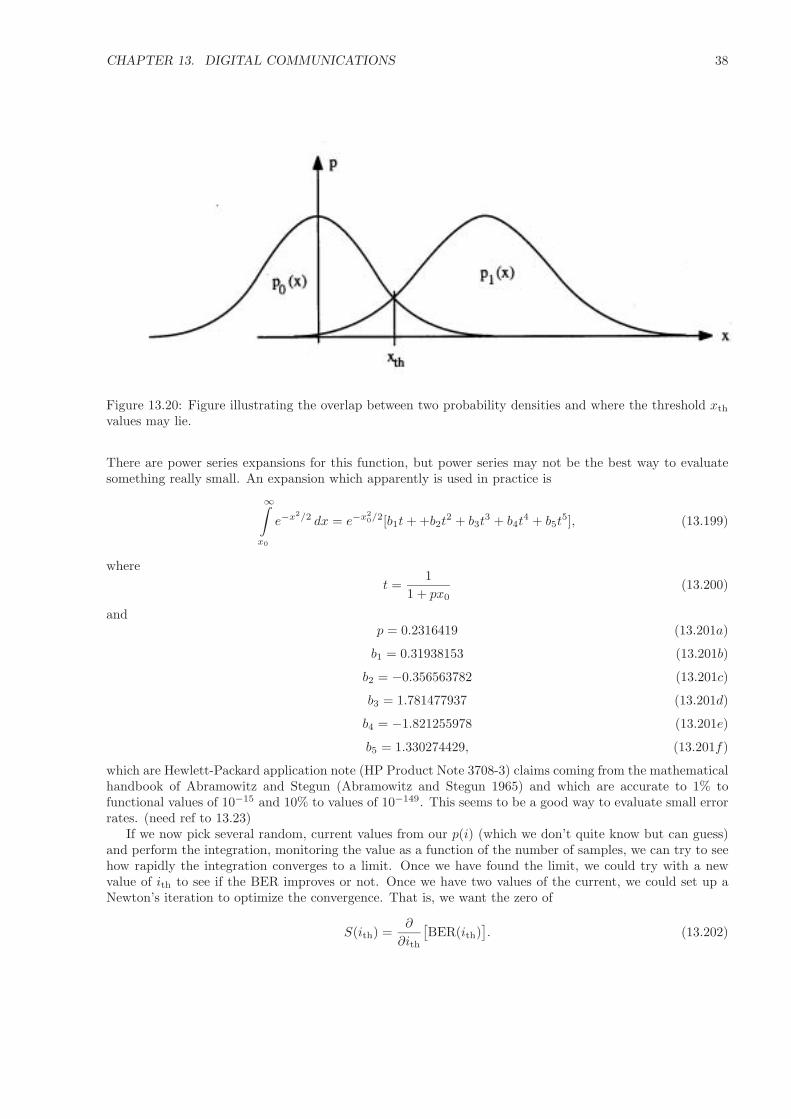
CHAPTER 13. DIGITAL COMMUNICATIONS 38
Figure 13.20: Figure illustrating the overlap between two probability densities and where the threshold xth
values may lie.
There are power series expansions for this function, but power series may not be the best way to evaluatesomething really small. An expansion which apparently is used in practice is
∞∫x0
e−x2/2 dx = e−x20/2[b1t + +b2t
2 + b3t3 + b4t
4 + b5t5], (13.199)
wheret =
11 + px0
(13.200)
andp = 0.2316419 (13.201a)
b1 = 0.31938153 (13.201b)
b2 = −0.356563782 (13.201c)
b3 = 1.781477937 (13.201d)
b4 = −1.821255978 (13.201e)
b5 = 1.330274429, (13.201f)
which are Hewlett-Packard application note (HP Product Note 3708-3) claims coming from the mathematicalhandbook of Abramowitz and Stegun (Abramowitz and Stegun 1965) and which are accurate to 1% tofunctional values of 10−15 and 10% to values of 10−149. This seems to be a good way to evaluate small errorrates. (need ref to 13.23)
If we now pick several random, current values from our p(i) (which we don’t quite know but can guess)and perform the integration, monitoring the value as a function of the number of samples, we can try to seehow rapidly the integration converges to a limit. Once we have found the limit, we could try with a newvalue of ith to see if the BER improves or not. Once we have two values of the current, we could set up aNewton’s iteration to optimize the convergence. That is, we want the zero of
S(ith) =∂
∂ith
[BER(ith)
]. (13.202)
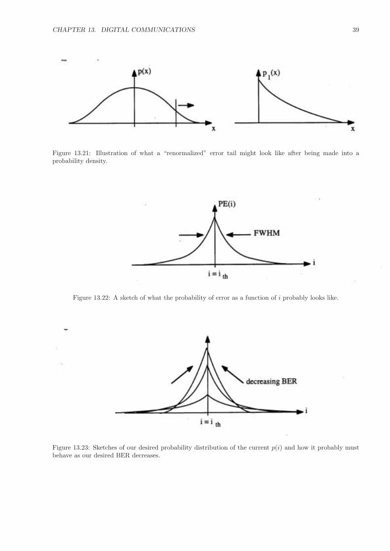
CHAPTER 13. DIGITAL COMMUNICATIONS 39
Figure 13.21: Illustration of what a “renormalized” error tail might look like after being made into aprobability density.
Figure 13.22: A sketch of what the probability of error as a function of i probably looks like.
Figure 13.23: Sketches of our desired probability distribution of the current p(i) and how it probably mustbehave as our desired BER decreases.
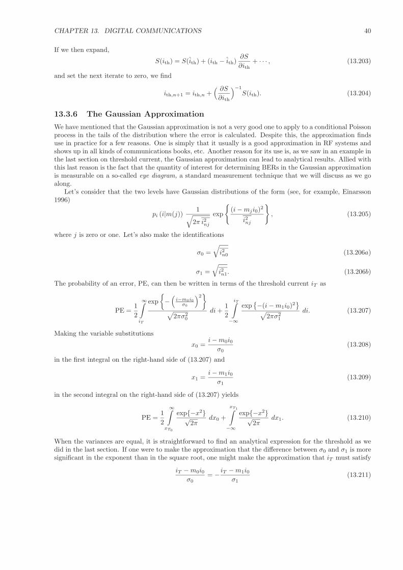
CHAPTER 13. DIGITAL COMMUNICATIONS 40
If we then expand,
S(ith) = S(ith) + (ith − ith)∂S
∂ith+ · · · , (13.203)
and set the next iterate to zero, we find
ith,n+1 = ith,n +( ∂S
∂ith
)−1
S(ith). (13.204)
13.3.6 The Gaussian Approximation
We have mentioned that the Gaussian approximation is not a very good one to apply to a conditional Poissonprocess in the tails of the distribution where the error is calculated. Despite this, the approximation findsuse in practice for a few reasons. One is simply that it usually is a good approximation in RF systems andshows up in all kinds of communications books, etc. Another reason for its use is, as we saw in an example inthe last section on threshold current, the Gaussian approximation can lead to analytical results. Allied withthis last reason is the fact that the quantity of interest for determining BERs in the Gaussian approximationis measurable on a so-called eye diagram, a standard measurement technique that we will discuss as we goalong.
Let’s consider that the two levels have Gaussian distributions of the form (see, for example, Einarsson1996)
pi (i|m(j))1√
2π i2nj
exp
(i − mji0)2
i2nj
, (13.205)
where j is zero or one. Let’s also make the identifications
σ0 =√
i2n0 (13.206a)
σ1 =√
i2n1. (13.206b)
The probability of an error, PE, can then be written in terms of the threshold current iT as
PE =12
∞∫iT
exp−(
i−m0i0σ0
)2
√2πσ2
0
di +12
iT∫−∞
exp−(i − m1i0)2
√2πσ2
1
di. (13.207)
Making the variable substitutions
x0 =i − m0i0
σ0(13.208)
in the first integral on the right-hand side of (13.207) and
x1 =i − m1i0
σ1(13.209)
in the second integral on the right-hand side of (13.207) yields
PE =12
∞∫xT0
exp−x2√2π
dx0 +
xT1∫−∞
exp−x2√2π
dx1. (13.210)
When the variances are equal, it is straightforward to find an analytical expression for the threshold as wedid in the last section. If one were to make the approximation that the difference between σ0 and σ1 is moresignificant in the exponent than in the square root, one might make the approximation that iT must satisfy
iT − m0i0σ0
= − iT − m1i0σ1
(13.211)

CHAPTER 13. DIGITAL COMMUNICATIONS 41
with solutioniT =
σ0m1 + σ1m0
σ0 + σ1i0. (13.212)
Clearly, for this choice of iT , the xT0 and xT1 of (13.210) above are given by
xT0 =m1 − m0
σ0 + σ1= −xT1
∆=Q, (13.213)
and therefore we can write
PE =12
∞∫Q
exp−x2√2π
dx +12
Q∫−∞
exp−x2√2π
, (13.214)
which in turn can be expressed in terms of the complementary error function erfc(x),
erfc(x) =1√2π
∞∫x
e−x2dx (13.215)
byPE = erfc(Q). (13.216)
It should be noted that, for Q ≥ 3, an accurate approximation to erfc(Q) is
erfc(Q) =1
Q√
2πe−Q2/2, (13.217)
which is a so-called Chernoff bound on the integral. Note that in the limit here of
m1 >> m0; σ1 >> σ0, (13.218)
the Q is just the optical SNR, as would be found from the pdf of the conditioning field, which correspondsto the square root of the SNR in terms of electrical power. The electrical SNR in dB can be obtained bysimply taking
SNRe = 20 log10 Q. (13.219)
We’ll next turn to a measurement technique which can find an approximate Q easily.
13.3.7 Eye Diagrams
In the past, a primary technique used to determine the threshold level was to simply pick a level, measure theBER, increment the level, measure the BER, etc., until the level was found where the BER is minimum. Fora telephone system with a required BER of 10−9 operating at a rate of 1 Gbs, a BER could be determinedwith some level of certainty in a few minutes. For data, such a BER is unacceptably high in many cases. Ata BER of 10−16 and a rate of 1 Gbs, there will be an error only every four months, and a BER determinationcould take decades. However, as explained in some detail by Bergano (Bergano et al 1993, Bergano andDavidson 1996, Bergano 1997), there is still a technique to find an approximate Q with which to approximatea BER.
An oft-used technique to estimate digital link performance is to observe the input to the decision circuitrywith a storage oscilloscope. Such a trace may appear as in the sketch of Figure 13.24, where it has beenassumed that the data is pseudo-random. On the eye diagram, we see four lines—one representing a samplingof the signal when no data transition takes place from 1 to 0, one for which there is no transition from 0,and two more where transitions do take place. As many bits have been sampled, noise on the trace causesthe traces to thicken and, therefore, the eye to close. The eye diagram is useful as a qualitative tool withoutany further analysis. However, one can go further. If one samples the trace values that have occurred atthe center of the eye, one can obtain pdf’s of the zeros and ones. If one has some reasonable certainty as towhat form the pdf’s should have (i.e. Gaussian), one can fit the data to the supposed pdf, determine freeparameters, and then extrapolate a BER. If one fits the distributions to Gaussians, the data can be used tofind m1, m0, σ0, σ1, and, therefore, Q.
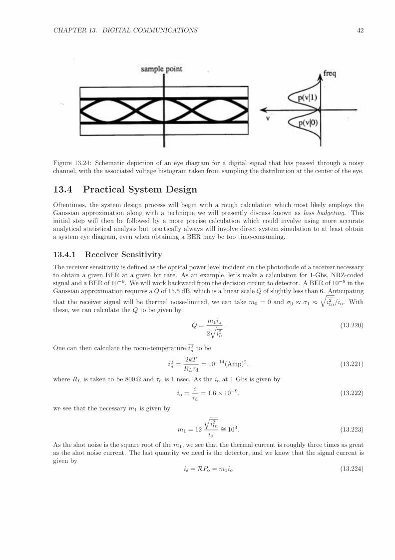
CHAPTER 13. DIGITAL COMMUNICATIONS 42
Figure 13.24: Schematic depiction of an eye diagram for a digital signal that has passed through a noisychannel, with the associated voltage histogram taken from sampling the distribution at the center of the eye.
13.4 Practical System Design
Oftentimes, the system design process will begin with a rough calculation which most likely employs theGaussian approximation along with a technique we will presently discuss known as loss budgeting. Thisinitial step will then be followed by a more precise calculation which could involve using more accurateanalytical statistical analysis but practically always will involve direct system simulation to at least obtaina system eye diagram, even when obtaining a BER may be too time-consuming.
13.4.1 Receiver Sensitivity
The receiver sensitivity is defined as the optical power level incident on the photodiode of a receiver necessaryto obtain a given BER at a given bit rate. As an example, let’s make a calculation for 1-Gbs, NRZ-codedsignal and a BER of 10−9. We will work backward from the decision circuit to detector. A BER of 10−9 in theGaussian approximation requires a Q of 15.5 dB, which is a linear scale Q of slightly less than 6. Anticipating
that the receiver signal will be thermal noise-limited, we can take m0 = 0 and σ0 ≈ σ1 ≈√
i2tn/io. Withthese, we can calculate the Q to be given by
Q =m1io
2√
i2n
. (13.220)
One can then calculate the room-temperature i2n to be
i2n =2kT
RLτd= 10−14(Amp)2, (13.221)
where RL is taken to be 800Ω and τd is 1 nsec. As the io at 1 Gbs is given by
io =e
τd= 1.6 × 10⁻⁹, (13.222)
we see that the necessary m1 is given by
m1 = 12
√i2tn
io∼= 103. (13.223)
As the shot noise is the square root of the m1, we see that the thermal current is roughly three times as greatas the shot noise current. The last quantity we need is the detector, and we know that the signal current isgiven by
is = RPo = m1io (13.224)

CHAPTER 13. DIGITAL COMMUNICATIONS 43
or, as R is given byR =
eη
hν, (13.225)
we see thatPo =
nν
eηm1io =
hν
ητdm1. (13.226)
At 1.55µm, hν is roughly 0.8 eV; η, however, is lower at 1.55µm than at shorter wavelengths, where it couldbe near unity, and could be as low as 0.2 eV. Plugging in, we find
Po = 7 × 10⁻⁷ W, (13.227)
so the receiver sensitivity is roughly 1µW or, in dBm,
Po = −30 dBm. (13.228)
13.4.2 Loss Budgeting
Knowing a receiver sensitivity, one can then ask all kinds of questions as, for a given fiber plant, how muchpower do we need? or, for a given launched power, how much loss can we take? If we knew the launchedpower, the fiber loss, and the total connector loss, we could find the total length possible. For example, let’ssay the laser can launch −10 dBm into the fiber. If one needs to acocunt for 2 dB of space, connector, anddetector coupling loss, then if the fiber loss is 0.2 dB/km, the link could be as long as 36 km. Of course,we did not take into account any BER margin—that is, although for perhaps 3 dB of extra power in thereceiver to account for inaccuracies and aging—that is, the components may change with time. We also didnot account for loss penalties.
13.4.3 Power Penalties
To present, the model has only taken into account loss. There are other propagation effects, most notablydispersion. In multimode fibers, this is relatively straightforwad, as modal dispersion dominates chromaticdispersion. A problem is the launch conditions. A manufacturer gives a rating in terms of MHz/km ofbandwidth, but multimode launches, other than overfilled ones, are hard to repeat. Even with an LED,no less a laser, it is hard to overfill the modes. In single-mode fiber, the problem is worse still, as withno modal dispersion there is only chromatic dispersion, and it starts out strongly dependent on the sourcespectrum. The spectrum may chirp, may exhibit mode partitioning, may be transform-limited, etc. Further,any nonlinear effects in the fiber such as self phase modulation will have an effect on the spectrum as thelight travels down the fiber. To top all of these off, some single-mode fibers can exhibit a large degreeof polarization mode dispersion, which is also quite spectrum-dependent. Probably the bottom line withdispersion, though, is that, if one knows the shape of the pulse entering the detector and from that cancalculate the amount of the pulse that does not fit within the decision time frame, this will affect the m1 andm0 values that were used in calculating the receiver sensitivity. Calculating the reduction in sensitivity dueto the time frame “slopover” gives a number in dB that is called the power penalty. Various texts discussthis (Agrawal 1992, Gower 1984, Einarsson 1996).
Another source of power penalty can be amplitude fluctuations. In multimode fibers, modal noise isa sourcewidth-dependent cause. In any system, laser RIN will cause additional modulation. The primaryeffect of the amplitude fluctuations is to increase the effective values of both the m1 and σ1 of the receiversensitivity.
13.5 Multiplexing Techniques
One wishes to always make a system that is upgradable—that is, whose data rate can be increased at afuture time without having to install a new cable plant. Although the price for bare fiber may be below$.20/meter, by the time right of way has been secured and the fiber cabled and installed, the cost may betwenty times that of the bare fiber. The cable plant for a 2-km trunk may cost in the tens of thousands of
CHAPTER 13. DIGITAL COMMUNICATIONS 44
dollars, while the price for an 80-km span of long line could approach $1 million. Telephone traffic increasesexponentially with time, so problems of overcapacity don’t last very long. This was the reason for the initialintroduction of fiber into the phone network. Twisted pair or even coax cable was not even upgradable fromDS1 (1.54 MHz) to DS1C (3.08 MHz) with two-kilometer spacing back in the early 1970s. Optical fibercould be upgraded to an order of magnitude beyond that. (See, for example, Personick 1993.)
13.5.1 Space-Division Multiplexing (SDM)
The easiest way to upgrade data throughput is to use more fibers. Generally, when fiber is installed, anumber of extra, unused fibers are put in for future use. There is a limit on the upgradability with thistechnique. One can install more fibers than necessary, but probably nothing like an order of magnitudemore. In an exponentially growing market, such upgrades do not last too long.
13.5.2 Time-Division Multiplexing (TDM)
As was mentioned previously, one can bit-interleave data coming in by using the fiber bandwidth. Althoughthe fiber bandwidth is large (> Tbs), it is not all accessible at present with TDM. The problem is transmitterand receiver electronics. When SONET/SDH standards became accepted, it was thought that the data rateswould rapidly increase from 625 Mbs to 2.5 Gbs to 10 Gbs and on to 40 Gbs. Although 10 Gbs (OC192)systems are beginning to appear, 40 Gbs looks a long way off. Not that many years ago, many telecos wereinvolved in making their own special electronics. In today’s market, where economics is a prime consideration,electronics being used are more often those of electronic component companys, as the production costs canbe lower with such concerns due to the volume of production. But this fact now ties the rate of TDMdevelopment to the market. There seem to be gradually increasing interest and availability of multi-gigabitcomponents, but one must doubt that 40 Gbs and 160 Gbs are going to appear in any quantity especiallysoon.
13.5.3 Wavelength-Division Multiplexing (WDM)
WDM is presently finding ways around the electronic problem by performing certain operations in the opticaldomain. A simple WDM system is depicted in Figure 13.25. The basic idea is that multiple channels canbe carried over a single fiber if each channel is at a separate known wavelength. This does require somesource stability, but by spacing the channels a distance much greater than the information bandwidth of anychannel as well as using external modulation of DFB lasers to minimize any signal chirp, the problem becomesmanageable. Generally, the multiplexer is simply a 3-dB coupler. There will of course be an obligatory 3-dBcoupling loss at this junction due to the brightness theorem. (See, for example, Mickelson 1992.) For systemswith many channels (that is, many wavelengths), the problem is exacerbated as the loss for 2N channels mustbe minimally 3N dB. However, these larger systems tend to use optical amplifiers, with one right behindthe junction and often another at the detector. It is possible to attempt to losslessly combine by usingdispersive elements, but there are alignment problems, etc. The demultiplexer needs dispersive elements,but it is easier to split things apart losslessly than to put them back together. A simple optical grating willspatially separate channels, although more elegant solutions (i.e. not requiring free space propagation) canbe fiber Bragg gratings or waveguide gratings in various waveguide crystals. After separation, the systemsimply appears as two separate receivers.
Dense WDM (DWDM) is a technology which combines space, time, and wavelength multiplexing toachieve huge throughputs and thereby a great degree of upgradability. Lucent’s Wavestar OS40 system haseight fibers, each carrying 16 channels of 2.5-Gbs TDM’d signals for a composite rate of 320 Gbs. Lucent’sOS400 system also has eight fibers but 80 channels, each capable of handling both OC48 (2.5 Gbs) andOC192 (10 Gbs) in order to achieve a composite bandwidth of 3.2 Tbs. The system consists of 80-km spansbetween EDFAs. It is unlikely that there are many users who need such high data throughputs at present,so the system is being sold as a basic system, and then upgrades will be sold when needed.
Some new problems arise with DWDM. A typical system schematic may appear as in Figure 13.26. Aproblem that arises is that the gain profile of an EDFA is not really flat. If there are multiple amplifiers,it could be that some channels will grow and others will attenuate. This leads to obvious problems at the

CHAPTER 13. DIGITAL COMMUNICATIONS 45
Figure 13.25: Schematic depiction of a two-channel WDM system.
receivers, but even before this it could lead to some channels saturating downstream amplifiers. However,one can preattenuate some of the channels with respect to the others by employing an equalizer. Generallywhat one does is to employ a composite Bragg grating before the input of the first amplifier. The gratingsare designed to cause some amount of channels’ power to be either reflected or coupled to radiation modes.In this manner, by carefully selecting the necessary attenuation profile, one can equalize the received powers.(See, for example, Bergano 1997.)
Another problem that arises is overall power level. Nonlinear effects such as self phase modulation areno worse in DWDM if the power of each channel is the same as in a smaller system. The problem effectwill be four-wave mixing. The issue with cross-channel effects is that they become much more prevalentbetween phase-matched channels. Operation of such a system at near the dispersion minimum of a fiber istherefore not an especially good idea, although it was the initial idea behind dispersion-shifted fiber (shiftedto put the dispersion minimum at 1.55µm, which is the loss minimum and the choice for DWDM operationbecause of the passband of the EDFAs). But one can compensate for the effects of dispersion by havingtwo different fibers in the cable plant, one with a minimum above the operating wavelength and one withdispersion minimum below the operating wavelength. This scheme can cancel most of the second-orderdispersion (Bergano 1997, Bergano and Davidson 1996).
A last problem is that of routing. It would be nice to be able to add and drop wavelengths from thestream directly in the optical domain. Numerous proposals for such routers have been made (Kewitsch et al1998, Nykolak et al 1997, Okamato et al 1996). It is probably still too early (1999) to tell which technologyor combination of technologies may be used, but it is clear that a fully programmable optical router couldlead to a whole new dimension in optical networking.
13.5.4 Code-Division Multiple Access (CDMA)
In the RF world, CDMA is a rather mature technology. It is much less so in optics. It is in a sense a blockcode. A bit is made up of a set of chips which are coded either in the time domain through time positions(direct sequence, or DS-CDMA), the frequency domain through changes in frequency between equi-spacedchips (frequency encoded, or FE-CDMA) or in both, as fast frequency hopping (FFH-CDMA; see, for example,Fethallah et al 1999). The reason it is called multiple access is that there can be a number of “orthogonal”codes, meaning that one can have a number of different channels on a line. The idea is usually to let eachreceiver communicate on only one code—that is, have a filter which only receives one code word from thecode book. To the present, optical CDMA operates in much the same way as optical WDM—that is, as atechnique to put more channels of data on a single fiber. The technology just has not come nearly as far asoptical WDM to the present but does have some promise.

CHAPTER 13. DIGITAL COMMUNICATIONS 46
Figure 13.26: A possible DWDM system configuration including amplification, dispersion compensation, anda wavelength switch which allows for a degree of routing.
13.6 Simulation
We previously mentioned Monte-Carlo simulation. Probably every organization involved in fiber optic re-search and development has their own simulation programs. There are also some commercial products avail-able at present. A company called BNED has a product called BroadNed. They last year (1998) mergedwith a company called Virtual Photonics and started to market a product called Opals. Hewlett-Packarddeveloped a tool called Photonic Systems Design. Recently the three companies started a joint venture forH-P to market what they call the Photonic Transmission Design Suite, which is a combination of essentiallyall of the above tools. These tools are quite expensive and probably bought primarily by consulting firmsthat rely on such tools for their livelihood. In this section, something will be said about the common threadsbetween different simulation tools.
One aspect of the simulation tools I have seen is their modularity. They are very much based on usingdifferent blocks that have inputs and outputs that are compatible with another set of blocks. In this sense(and others), they follow the recommendations of books such as Jeruchim et al (1992) on simulation ofcommunication systems. An example of a system block diagram for a channel of a DWDM system mightappear as in Figure 13.27. The clock block would be input a rate and perhaps pulse (code) shapes to begated ON and OFF by a pseudo-random sequence generator. The sequence generator would be limited insuch things as the length of the sequence. The laser block could be complicated or simple. It could begiven such information as RIN and spectral width alone, or the information could be as complex as a rateequation simulation. Even though an electroabsorption external modulator is included, generally the EAMis monolithic, causing laser chirp. The EAM will also exhibit dynamic chirp due to the changing refractiveindex in the medium. These effects change according to the operating point of the laser as well as the signalmodulation depth and, evidently, the modulation characteristic of the EAM. Unless the simulation calculatesthese things from fabrication parameters, these parameters all must be input. Oftentimes a filter is usedbefore the first link in order to shape the pulse. Pulse shape can be quite important in nonlinear propagation.Evidently the filter characteristic must be input. The signal flow then enters the first link. Coupling efficiencyshould somehow be included. The fiber loss, second-order dispersion, and nonlinear coefficient need to beinput if all the pertinent propagation effects are to be taken into account. Some amplified simulationsinput only loss, as in long links the integration of the nonlinear equations can be quite time-consuming.

CHAPTER 13. DIGITAL COMMUNICATIONS 47
Signal flow through the erbium-doped fiber amplifier (EDFA) can also become computer-intensive, as thesignal, pump, and ASE satisfy a complicated nonlinear equation involving all fiber parameters including allrelevant dopant profiles. The detector preamplifier combination requires knowledge of detector efficiency,dark current, and an overall electrical transfer function including capacitor junction capacitance. There arenumerous clock recovery/decision circuits available, and, as this is the crucial step, they need to be wellmodeled. Evidently, much work needs to go into keeping the blocks up to date on components and devices.There is also a question about what level of approximation one uses in the modeling. Simulating a DWDMsystem using time-resolved spectra of lasers, full nonlinear propagation, could probably take days on a PCif the PC didn’t crash first. One has to pick and choose. This is not, however, just a property of opticalsimulators. Hewlett-Packard’s MDS uses reasonably simple lookup models and runs reasonably quickly ona workstation. The same can’t really be said for full wave simulators like H-P’s HFSS. One way in whichdigital circuit simulation tools have somewhat circumvented such problems is by being hierarchical as well asmodular. If “standard” models programmed into the simulators are good enough to meet specifications, thenone might be able to complete a design with chips modeled simply by transfer functions (or, more correctly,logic operations). If such doesn’t work, one needs to find the offensive piece (chip) and do internal modelingof pieces inside the chip as transfer functions. If one really needs to do something in a custom manner, onemay need to drop five or more levels (depending on the simulator) and go all the way to the transistor level.With ten million transistors in a chip and several chips in a system, such is not terribly productive. Opticalsimulation (or analog, for that matter) is nowhere near the level of hierarchical simulation at this point intime.
As anyone who has used SPICE or MDS is aware, when modeling something real, one’s simulation resultis only as good as the set of parameter models in one’s version. Student versions of simulators can beinexpensive, but the device models tend to be primitive. The most recent models probably only exist infoundries or are obtained at great expense by consultants being paid for design. The same is somewhat truewith optical simulation. Even if you had a simulator, a system simulation requires a multitude of parametersfrom the detail of the source chirp spectra to the time constants in the clock recovery circuit. This makessimulation a good tool for use the in the R&D lab but less useful for modeling some strange behavior in asystem whose parameters are not well documented or maybe even proprietary. But again, this problem isnot unique to optical simulation.
Problems
1. As in problem 13.1 above, assume that the current to be MAP decoded is made up of signal, shotnoise, and dark and thermal current. Assume that there are timing errors of order ε for one period.
(a) Calculate the effects of a timing error on the SNRp calculated in problem 1(a) above. Sketch thisSNRp for several values of ε between 0 and 0.5. What happens if ε > 0.5?
(b) In a real practical optical communications system, one would try to control the BER due to timingerrors to be about as large as the BER due to the largest noise-producing source in the receiver.In general, a control system which can place a timing spike with accuracy ε within a period T of asignal of bandwidth B will require a bandwidth of B/ε. Calculate the control system bandwidthsnecessary for “practical” communication systems operating in the following regimes:
i. αPs < αPd;ii. αPd < αPs < Nt/e2;iii. e2α2P 2
s > Nt2B > e2αPs2B.
2. Consider two Gaussian distributed intensity levels:
PI0(I0) =1√
2π σ0
exp−(I0 − 〈I0〉
)22σ2
0
PI1(I1) =1√
2π σ1
exp−(I1 − 〈I1〉
)22σ2
1
.

CHAPTER 13. DIGITAL COMMUNICATIONS 48
Figure 13.27: Schematic of the simulation blocks that might be used to simulate a single channel of a DWDM.Blocks are discussed in the text.
Find an expression defining an optimal decision threshold intensity It for differentiating between thesetwo levels. Explain why your It is optimal. Find It in the limit where σ1 = σ0.
3. Assume that k is distributed by a negative binomial variate distribution for either of its two possiblelogical states, k0 and k1. In what follows, assume that the lower level is defined by k0 = 0 and theupper state is high enough to achieve a reasonable BER. Further assume that the coding is such thatzeroes and ones are equally likely in the incident stream.
(a) Find an expression satisfied by the ML kT for an ML realization of a MAP decoder.Specialize the kT in (a) to the cases where
(b) N → 1 and where
(c) N >> 1.In both cases, give expressions for the BER.
(d) Repeat (c) for the cases where k0 = 1.
4. Consider a two-mode fiber with modal group velocities Vg1 and Vg2. Say that a sequence of 1s and 0sis transmitted over the fiber. Find the probability of error, PE due only to this dispersion in terms of∆Vg = Vg2 − Vg1. Explain your method of attack in this problem.

Bibliography
[1] M. Abramowitz and I. A. Stegun, Handbook of Mathematical Functions (Dover Publications, 1965).
[2] G. P. Agrawal, Fiber Optic Communication Systems (New York: Wiley, 1992).
[3] Zh. I. Alferov, M. V. Andreev, E. L. Portnoi, and M. K. Trukan, “AlAs-GaAs HeterojunctionInjection Lasers with a Low Room-Temperature Threshold,” Sov Phys Semiconductors 3, 1107-1110 (1970).
[4] J. Bardeen and W. H. Brittain, “The Transistor, a Semiconductor Triode,” Phys Rev 74, 230(1948).
[5] N. G. Basov, O. N. Krokhin, and Y. M. Popov, “Production of Negative Temperature States inp − n Junctions of Degenerate Semiconductors,” J E T P 40, 1320 (1961).
[6] N. S. Bergano, “Undersea Amplified Lightwave Systems Design,” in Optical Fiber Telecommuni-cations, Vol. IIIA, I. P. Kaminow and T. L. Koch, Eds. (Murray Hill, NJ: Lucent Technologies,1997).
[7] N. S. Bergano and C. R. Davidson, “Wavelength Division Multiplexing in Long-Haul TransmissionSystems,” Journ Light Tech 19:1299–1308 (1996).
[8] N. S. Bergano, F. W. Kerfoot, and C. R. Davidson, “Margin Measurement in Optical AmplifierSystems,” IEEE Photon Tech Lett ??:304–306 (1993).
[9] D. L. Butler, J. S. Wey, M. W. Cubat, G. L. Burdge, and J. Goldhar, “Optical Clock Recoveryfrom a Data Stream of Arbitrary Bit Rate by Use of Stimulated Brillonin Scattering,” Optics Lett20:560–562 (1995).
[10] G. Einarsson, Lightwave Communications (New York: Wiley, 1996).
[11] H. Fathallah, L. A. Rusch, and S. LaRochelle, “Passive Optical Fast Frequency Hop CDMA Com-munications System,” to appear, Journ Light Tech (1999).
[12] T. K. Fong, M. Cerisola, R. T. Hofmeister, P. Poggiolini, and L. G. Kazovsky, “Ultrafast RecoveryTechnique for High Speed Optical Packet Networks,” Elect Lett 31:1687–1688 (1995).
[13] R. M. Gagliardi and S. Karp, Optical Communications, Second Edition (New York: Wiley, 1995).
[14] J. Gower, Optical Communications Systems (Prentice Hall, 1984).
[15] H. Haken, Light, Volume 1: Waves, Photons, Atoms (North Holland, 1981).
[16] H. Haken, Light, Volume 2: Laser Light Dynamics (North Holland, 1985).
[17] R. N. Hall, G. E. Fenner, J. O. Kingsley, T. J. Soltys, and R. O. Carlson, “Coherent Light Emissionfor GaAs Junctions,” Phys Dev Lett 9, 366 (1962).
[18] I. Hayashi and M. B. Panish, “GaAs-GaxAl1−xAs Heterostructure Injection Lasers which ExhibitLow Thresholds at Room Temperature,” J Appl Phys 41, 150–163 (1970).
49
BIBLIOGRAPHY 50
[19] K. O. Hill and G. Meltz, “Fiber Bragg Grating Technology Fundamentals and Overview,” JournLight Tech 15:1263–1276 (1997).
[20] D. Hondros and P. Debye, “Elektromagnetische Wellen an Dielektrischen Drahten,” Ann Phys 32,465–476 (1910).
[21] Y. Imai, E. Sano, M. Nakumura, N. Ishihara, H. Kikuchi, and T. Ono, “Design and Performanceof Clock-Recovery GaAs ICs for High-Speed Optical Communication Systems,” IEEE Trans Mi-crowave Th Tech 41:745–751 (1993).
[22] jeru92 M. C. Jeruchim, P. Balaban, and K. S. Shanmugon, Simulation of Communication Systems(New York: Plenum Press, 1992).
[23] F. P. Kapron, D. B. Keck, and R. D. Maurer, “Radiation Losses in Glass Optical Waveguides,”Appl Phys Lett 17, 423-425 (1970).
[24] S. Kawanishi and M. Saruwatori, “Ultra-High-Speed PLL-Type Clock Recovery Circuit Based onAll-Optical Gain Modulation in Traveling-Wave Laser Diode Amplifier,” IEEE Journ Light Tech11:2123–2129 (1993).
[25] G. Keiser, Optical Fiber Communications, First Edition (McGraw-Hill, 1983) and Second Edition(1991).
[26] A. S. Kewitsch, G. A. Rakuljic, P. A. Willems, and A. Yariv, “All-Fiber Zero-Insertion-Loss Add-Drop Filter for Wavelength Division Multiplexing,” Opt Lett 23:106–108 (1998).
[27] C. J. Koester and E. Snitzer, “Amplification in a Barium Crown Glass,” Appl Opt 3, 1182–1186(1964).
[28] G. Lenz, B. J. Eggleton, C. R. Giles, C. K. Madsen, and R. E. Slusher, “Dispersive Properties ofOptical Filters for WDM Systems,” IEEE Journ Quant Elect 34:1390–1402 (1998).
[29] T. H. Maimon, “Optical and Microwave-Optical Experiments in Ruby,” Phys Rev Lett 4, 564–565(1960).
[30] A. R. Mickelson, Guided Wave Optics (Van Nostrand, 1993).
[31] D. Middleton, An Introduction to Statistical Communication Theory (McGraw-Hill, 1960); re-printed (Peninsula, 1987); reprinted (IEEE Press, 1996).
[32] M. I. Nathan, W. P. Dumke, G. Burns, F. H. Dills, and G. Lasher, “Stimulated Emission ofRadiation from GaAs p − n Junctions,” Appl Phys Lett 1, 62 (1962).
[33] G. Nykokak, M. R. X. deBarros, T. N. Nielsen, and L. Eskildsen, “All-Fiber Active Add-DropWavelength Router,” IEEE Photon Tech Lett 9:605–606 (1997).
[34] H. Nyquist, “Certain Topics in Telegraph Transmission Theory,” Trans AIEE 47, 617–644 (1928).
[35] K. Okavisto, M. Okuno, A. Hinens, and Y. Ohmori, “16-Channel Optical Add/Drop MultiplexerConsisting of Arrayed-Waveguide Gratings and Double-Gate Switches,” Opt Lett 32:1471–1472(1996).
[36] G. Orsak and B. Aazhang, “On the Theory of Importance Sampling Applied to the Analysis ofDetection Systems,” IEEE Trans Comm 37, 332-339 (1989).
[37] G. Orsak and B. Aazhang, “Constrained Solutions in Importance Sampling via Robust Statistics,”IEEE Trans Inform Th 37, 307–316 (1991).
[38] G. Orsak and B. Aazhang, “A Class of Optimum Importance Sampling Strategies,” InformationSciences 84, 139–160 (1995).
BIBLIOGRAPHY 51
[39] S. Personick, “Towards Global Information Networking,” Proc IEEE 81(11), 1549 (1993).
[40] A. Pottbacker, U. Langmann, and H.-U. Schreider, “A Si Bipolar Phase and Frequency DetectorIC for Clock Extraction up to 8 Gb/s,” IEEE Journ Solid-State Circuits 27:1747–1751 (1992).
[41] J. W. S. Rayleigh, Phil Mag 43, 125 (1897).
[42] L. L. Scharf, Statistical Signal Processing: Detection, Estimation, and Time Series Analysis(Addison-Wesley Publishing Co., 1991).
[43] W. Schockley, “The Theory of p−n Junctions in Semiconductors and p−n Junction Transistors,”Bell Sys Tech Journ 28, 435 (1949).
[44] O. Schriever, “Elektromagnetische Wellen and Dielektrischen Drahten,” Ann Phys 64, 645–673(1920).
[45] M. Schwartz, Information, Transmission Modulation, and Noise (New York: McGraw-Hill, 1970).
[46] M. Schwartz, W. R. Bennett, and S. Stein, Communication Systems and Techniques (McGraw-Hill,1966); reprinted (IEEE Press, 1996).
[47] C. E. Shannon, “A Mathematical Theory of Communication,” Bell Sys Tech Journ 27, 379–423(Part I), 623–656 (Part II). Reprinted in book form with postscript by W. Weaver (Urbana: Uni-versity of Illinois Press, 1949).
[48] C. E. Shannon, “Probability of Error for Optimal Codes in a Gaussian Channel,” Bell Sys TechJourn 38, 611–656 (1959).
[49] E. Snitzer, “Cylindrical Dielectric Waveguide Modes,” J Opt Soc Amer 51, 491–498 (1961a).
[50] E. Snitzer, “Optical Maser Action of Nd+3 in a Barium Crown Glass,” Phys Rev Lett 7, 444-446(1961b).
[51] A. Sommerfeld, Ann d Phys 67, 233 (1899).
[52] A. M. Vengsarkar, P. J. Lemaire, J. B. Judkins, V. Bhatia, T. Erdogan, and J. E. Sipe, “Long-PeriodFiber Gratings as Band-Rejection Filters,” Journ Light Tech 14:58–68 (1996).
[53] L. J. Wang, H. X. Shi, J. T. Lin, K. J. Gua, and P. Ye, “Clock and Frame Synchronization RecoveryBased on a Terrahertz Asymmetric Demultiplexer,” IEEE Photon Tech Lett 10:881–883 (1998).
[54] E. T. Whittaker, “On the Functions which are Represented by the Expansions of the InterpolationTheory,” Proc Royal Soc Edinburgh 35, 181–195 (1915).
[55] J. Xu and R. Strand, Acouto-Optic Devices: Principles, Design, and Applications (New York:Wiley, 1992).
[56] H. Zahn, “Uber den Nachweis Elektromagnetischen Wellen an Dielektrischen Drahten,” Ann Phys49, 907–933 (1916).