Digital Control and Monitoring Methods for

Nonlinear Processes

A ThesisPresented to

The Academic Faculty

by

Nguyen Huynh

In Partial Fulfillmentof the Requirements for the Degree

Doctor of Philosophy

Chemical EngineeringWorcester Polytechnic Institute

September 2006

ABSTRACT

The chemical engineering literature is dominated by physical and (bio)-

chemical processes that exhibit complex nonlinear behavior, and as a consequence, the

associated requirements of their analysis, optimization, control and monitoring pose

considerable challenges in the face of emerging competitive pressures on the chemical,

petrochemical and pharmaceutical industries. The above operational requirements

are now increasingly imposed on processes that exhibit inherently nonlinear behavior

over a wide range of operating conditions, rendering the employment of linear process

control and monitoring methods rather inadequate. At the same time, increased

research efforts are now concentrated on the development of new process control and

supervisory systems that could be digitally implemented with the aid of powerful

computer software codes. In particular, it is widely recognized that the important

objective of process performance reliability can be met through a comprehensive

framework for process control and monitoring. From:

(i) a process safety point of view, the more reliable the process control and monitor-

ing scheme employed and the earlier the detection of an operationally hazardous

problem, the greater the intervening power of the process engineering team to

correct it and restore operational order

iii

(ii) a product quality point of view, the earlier detection of an operational prob-

lem might prevent the unnecessary production of off-spec products, and subse-

quently minimize cost.

The present work proposes a new methodological perspective and a novel set of

systematic analytical tools aiming at the synthesis and tuning of well-performing dig-

ital controllers and the development of monitoring algorithms for nonlinear processes.

In particular, the main thematic and research axis traced are:

(i) The systematic integrated synthesis and tuning of advanced model-based digital

controllers using techniques conceptually inspired by Zubov’s advanced stability

theory.

(ii) The rigorous quantitative characterization and monitoring of the asymptotic

behavior of complex nonlinear processes using the notion of invariant manifolds

and functional equations theory.

(iii) The systematic design of nonlinear state observer-based process monitoring sys-

tems to accurately reconstruct unmeasurable process variables in the presence

of time-scale multiplicity.

(iv) The design of robust nonlinear digital observers for chemical reaction systems

in the presence of model uncertainty.

iv

ACKNOWLEDGEMENTS

First, I would like to give my sincere thanks to my advisor, Professor Nikolaos

Kazantzis, for his support, insight and guidance throughout this project.

Thanks to my thesis committee for accepting to read this work.

Thanks the Department of Chemical Engineering, its faculty, staff and students

for their warm welcome.

Thanks to my friends and family, here and there.

Special thoughts for Fede, Matt, Philippe, Wat, Fred, Nancy, Pascal, James, Jean,

Florin, Tracy, Raphael, Magali, Nicolas, Claire, le petit Camille, Jean-Louis, Michael,

Florent, Martin, Therese, Madee, Ann, Velocity, Remi, Isabelle, Jacqueline, Papa et

Maman.

v

TABLE OF CONTENTS

ABSTRACT . . . . . . . . . . . . . . . . . . . . . . . . . . . . . . . . . . . iii

ACKNOWLEDGEMENTS . . . . . . . . . . . . . . . . . . . . . . . . . . v

TABLE OF CONTENTS . . . . . . . . . . . . . . . . . . . . . . . . . . . vi

LIST OF TABLES . . . . . . . . . . . . . . . . . . . . . . . . . . . . . . . viii

LIST OF TABLES . . . . . . . . . . . . . . . . . . . . . . . . . . . . . . . . viii

LIST OF FIGURES . . . . . . . . . . . . . . . . . . . . . . . . . . . . . . ix

LIST OF FIGURES . . . . . . . . . . . . . . . . . . . . . . . . . . . . . . . ix

I PARAMETRIC OPTIMIZATION OF DIGITALLY CONTROLLEDNONLINEAR REACTOR DYNAMICS . . . . . . . . . . . . . . . 1

1.1 Introduction . . . . . . . . . . . . . . . . . . . . . . . . . . . . . . . 1

1.2 Mathematical Preliminaries and Motivation . . . . . . . . . . . . . . 4

1.3 The Proposed Approach . . . . . . . . . . . . . . . . . . . . . . . . . 12

1.4 Illustrative example . . . . . . . . . . . . . . . . . . . . . . . . . . . 16

1.5 Concluding Remarks . . . . . . . . . . . . . . . . . . . . . . . . . . . 22

II A MODEL-BASED CHARACTERIZATION OF THE LONG TERMASYMPTOTIC BEHAVIOR OF NONLINEAR DISCRETE-TIMEPROCESSES . . . . . . . . . . . . . . . . . . . . . . . . . . . . . . . . 24

2.1 Introduction . . . . . . . . . . . . . . . . . . . . . . . . . . . . . . . 24

2.2 Mathematical preliminaries . . . . . . . . . . . . . . . . . . . . . . . 27

2.3 Main results . . . . . . . . . . . . . . . . . . . . . . . . . . . . . . . 29

vi

2.3.1 Special Case: The Long-Term Dynamic Behavior of LinearDiscrete-Time Processes . . . . . . . . . . . . . . . . . . . . 37

2.4 Illustrative example . . . . . . . . . . . . . . . . . . . . . . . . . . . 39

2.5 Concluding remarks . . . . . . . . . . . . . . . . . . . . . . . . . . . 44

III NONLINEAR OBSERVER DESIGN FOR PROCESS MONITOR-ING IN THE PRESENCE OF TIME-SCALE MULTIPLICITY 46

3.1 Introduction . . . . . . . . . . . . . . . . . . . . . . . . . . . . . . . 46

3.2 Mathematical preliminaries and problem formulation . . . . . . . . . 49

3.3 Main results . . . . . . . . . . . . . . . . . . . . . . . . . . . . . . . 55

3.4 Illustrative example . . . . . . . . . . . . . . . . . . . . . . . . . . . 61

3.5 Concluding remarks . . . . . . . . . . . . . . . . . . . . . . . . . . . 66

IV DISCRETE-TIME NONLINEAR OBSERVER DESIGN FOR CHEM-ICAL REACTION SYSTEMS IN THE PRESENCE OF MODELUNCERTAINTY . . . . . . . . . . . . . . . . . . . . . . . . . . . . . . 68

4.1 Introduction . . . . . . . . . . . . . . . . . . . . . . . . . . . . . . . 68

4.2 Mathematical preliminaries and problem formulation . . . . . . . . . 71

4.3 Main results . . . . . . . . . . . . . . . . . . . . . . . . . . . . . . . 76

4.4 Concluding remarks . . . . . . . . . . . . . . . . . . . . . . . . . . . 81

V CONCLUSIONS . . . . . . . . . . . . . . . . . . . . . . . . . . . . . . 83

I MAPLE CODE FOR CHAPTER II ILLUSTRATIVE EXAMPLE 87

II EXISTENCE AND UNIQUENESS CONDITIONS FOR THE SO-LUTION OF THE SYSTEM OF SINGULAR PDES (3.6) . . . . 89

REFERENCES . . . . . . . . . . . . . . . . . . . . . . . . . . . . . . . . . . 92

Bibliography . . . . . . . . . . . . . . . . . . . . . . . . . . . . . . . . . . . 92

vii

LIST OF TABLES

1 Process Parameter Values . . . . . . . . . . . . . . . . . . . . . . . . 18

2 Kinetic and bioreactor parameter values . . . . . . . . . . . . . . . . 40

viii

LIST OF FIGURES

1.1 Optimal values of p1 as a function of the size of the step change in theset point . . . . . . . . . . . . . . . . . . . . . . . . . . . . . . . . . 19

1.2 Optimal values of p2 as a function of the size of the step change in theset point . . . . . . . . . . . . . . . . . . . . . . . . . . . . . . . . . 20

1.3 Optimal output responses to a step change in the set point from 1.2gmol/lto 1.05gmol/l with different weight coefficient . . . . . . . . . . . . . 21

1.4 Optimal intput responses to a step change in the set point from 1.2gmol/lto 1.05gmol/l with different weight coefficient . . . . . . . . . . . . . 22

1.5 Geometric interpretation of the method for estimating the stabilityregion with N = 4, p1 = 46.4l2/h ·mol, p2 = 57.3l2/h ·mol . . . . . . 23

1.6 Stability region estimates for N = 2 and N = 4 with p1 = 46.4l2/h ·mol, p2 = 57.3l2/h ·mol . . . . . . . . . . . . . . . . . . . . . . . . . 23

2.1 Phaseportrait of the bioreactor dynamics slow manifold (N = 5). . . . 42

2.2 Phaseportrait of the bioreactor dynamics slow manifold (N = 10). . . 43

2.3 Comparison between the actual and estimated substrate concentrationprofiles (N = 10). . . . . . . . . . . . . . . . . . . . . . . . . . . . . . 44

2.4 Comparison between the actual and estimated substrate conversionprofiles (N = 10). . . . . . . . . . . . . . . . . . . . . . . . . . . . . . 45

3.1 Estimation of substrate concentration for ε = 2% of the fastest processtime-constant. . . . . . . . . . . . . . . . . . . . . . . . . . . . . . . . 64

3.2 Estimation of substrate concentration for ε = 30% of the fastest processtime-constant. . . . . . . . . . . . . . . . . . . . . . . . . . . . . . . . 65

3.3 Estimation of substrate concentration for ε comparable in magnitudeto the fastest process time-constant. . . . . . . . . . . . . . . . . . . . 67

ix

CHAPTER 1Parametric Optimization of Digitally

Controlled Nonlinear Reactor Dynamics

1.1 Introduction

In recent years, the development of powerful analytical and computational tools

enabled the analysis of the dynamic behavior of complex nonlinear chemical reaction

systems to be performed in a thorough and rigorous manner [42, 43, 86, 95]. As a

result, the ”inverse problem” of modifying and controlling the above dynamic be-

havior has also received considerable attention [18, 28]. In particular, it is widely

recognized that quite often the chemical reactor dynamics is often driven by ”input”

variables associated with the reactor feeding and reaction initiation policy (feed flow

rates, reactant inlet concentration, etc.), and therefore it is amenable to modification

through feedback action and the subsequent enforcement of the desirable dynamic

modes and behavior [18, 28]. Equivalently stated, one may derive a feedback control

law that dictates the appropriate input profile, which in turn, enforces the requisite

and desirable dynamic behavior on the controlled reactor dynamics. In particular,

unexpected disturbances may occur driving the chemical reactor far from the design

steady state conditions, and the primary objective is to derive a control law capable

1

of driving the system back to the design steady-state in a smooth, fast and reliable

manner, thus rejecting the disturbance effect [18,28].

The above represents a typical scenario of a reactor regulation problem that can

be adequately addressed via the action of a feedback controller. Please notice, that a

feedback regulator enjoys design flexibility by introducing tunable controller param-

eters that can be adjusted in order to assign the desirable dynamic characteristics

to the controlled reactor dynamics (speed and non-oscillatory characteristics of the

reactor’s response, tolerable overshoot, size of the stability region, transient behavior

towards the stable manifold, as well as other asymptotic properties) [18, 48].

Over the last two decades significant research effort has concentrated on the non-

linear feedback controller synthesis problem, in order to overcome performance limi-

tations associated with linear controller design methods applied to linearized reactor

dynamic models [18,48]. Furthermore, the advent of digital technology revolutionized

the way advanced nonlinear feedback control algorithms are implemented in practice

with the aid of a computer. Nowadays, computer-based digital control systems are

successfully designed and used in a multitude of applications [57, 78]. However, the

problem of systematically selecting the digital controller parameters for nonlinear

chemical reactors has not been given proper attention, and has been traditionally

addressed either through heuristics or trial-and-error type of approaches, thus in-

evitably resorting to extensive dynamic simulations and/or costly experiments [51,78].

The proposed approach aims at the development of a systematic and comprehensive

method to optimally select the parameters of a nonlinear digital reactor control sys-

tem, when in addition to standard performance requirements of the controlled reactor

dynamics (stability, fast and smooth regulatory response and disturbance rejection),

optimality is also requested with respect to a physically meaningful performance in-

dex.

2

In the present study [47], the tunable parameters of the feedback controlled reac-

tor dynamics are optimally selected through the minimization of a performance index,

representing the decision variables of the associated optimization problem. Under this

formulation, the problem under consideration becomes a finite-dimensional static op-

timization problem, as opposed to an infinite-dimensional nonlinear optimal control

problem that could exhibit computational challenges in practice [10]. Traditionally,

the above optimization problem is carried out in a ”brute force” manner: after an

initial guess for the controller parameters, the dynamic equations of the controlled

reactor dynamics are simulated and the value of the performance functional is calcu-

lated numerically. Then, a gradient-direction method is typically applied to update

the controller parameter values until convergence of the recursive algorithm leads to

an optimal set of controller parameter values [10]. More elaborate methods from

an algorithmic and computational point of view have also appeared in the pertinent

body of literature. They rely either on numerical techniques for solving challenging

two-point boundary value problems, or large scale nonlinear mathematical programs

resulting from time-discretization and parameterization of the input variables [10,31].

The present research study introduces a systematic and practical methodology

that addresses the above finite-dimensional static parametric optimization problem

for digitally controlled nonlinear reactor dynamics. In particular, the proposed ap-

proach is based on the explicit calculation of a physically meaningful quadratic per-

formance index by solving a Zubov-like functional equation. It can be proven that the

functional equation admits a unique locally analytic solution in the vicinity of the ref-

erence equilibrium point, which is also endowed with all the properties of a Lyapunov

function for the controlled reactor dynamics. Therefore, a transparent and very use-

ful link between optimality and stability can be established through the solution of

the above functional equation. Furthermore, the analyticity of the solution enables

the development of a series solution method for the functional equation that can be

3

easily implemented with the aid of a symbolic software package such as MAPLE. It

is also shown that the evaluation of the above Lyapunov function solution at the ini-

tial conditions leads to an explicit calculation of the value of the performance index.

Since the dynamic equations of the controlled reactor dynamics are parameterized

by the controller parameters, the Lyapunov function and solution to the functional

equation is also parameterized, and therefore, the value of the performance index

depends explicitly on the controller parameters. In light of the above observation,

the employment of static optimization techniques can provide the optimal values of

the finite set of controller parameters. Moreover, it should be pointed out, that for

the optimally calculated controller parameter values, an explicit estimate of the size

of the system’s stability region can also be provided by using results from advanced

stability theory for discrete dynamical systems [27,80].

The present chapter is organized as follows: In Section 1.2 a succinct description

of the requisite mathematical preliminaries and background is provided. Section 1.3

encompasses the main ideas and algorithmic structure of the proposed approach for

parametric optimization of nonlinear digitally controlled reactor dynamics. In Sec-

tion 1.4 simulation studies have been conducted in a representative chemical reactor

example in order to evaluate the proposed method and illustrate its applicability.

Finally, a few concluding remarks are provided in Section 1.5.

1.2 Mathematical Preliminaries and Motivation

Before we embark on the presentation of the proposed parametric optimization

scheme for nonlinear digitally controlled reactor dynamics, let’s first consider the

simpler case of linear reactor dynamics in order to conceptually and methodologically

motivate the development of its nonlinear analogue. The latter represents the focus of

the present study. A linear (or linearized) autonomous dynamic system is considered

4

in the discrete-time domain:

x(k + 1) = Ax(k) (1.1)

where the non-negative integer k ∈ N = 1, 2, ... is the discrete time index, x(k) ∈ Rn

is the vector of state variables at the time instant k and A an n× n constant matrix.

The above linear dynamic system in the discrete-time domain represents the linear

discrete dynamics of a chemical reactor that is obtained either:

• through a reliable and accurate discretization method applied to the original

continuous-time reactor dynamics in order to digitally (numerically) simulate

the dynamic behavior of the reactor of interest [18,52,78]

or:

• through direct system identification methods and a set of historical input/output

data, in the case where the reactor dynamics and the associated kinetics are dis-

couragingly complex and not amenable to first-principle based modeling [18,78].

In both cases however, it is assumed that equation (1.1) adequately captures

the actual linear reactor dynamics.

It is also assumed that the above system’s characteristic matrix A has stable

eigenvalues, which were assigned thanks to a fixed structure linear controller, designed

in accordance to well-known methods [48,78].

The following quadratic performance index associated with system (1.1) can be

defined:

J =∞∑

k=0

[x(k)]T Q [x(k)] (1.2)

where Q is an arbitrarily selected positive-definite symmetric matrix, and the super-

script T denotes the transpose of a vector or a matrix. Notice, that the aforementioned

stability requirement on the reactor dynamics (1.1) implies that the infinite series in

(1.2) converges to a fixed value limit [27,80].

5

Introducing the following Lyapunov matrix equation:

AT PA− P = Q (1.3)

one can easily show that equation (1.3) admits a unique symmetric and positive-

definite solution P [27]. Furthermore, applying standard Lyapunov stability theorems

[27], it can be inferred that the quadratic form defined below:

V (x) = xT Px (1.4)

has the following properties:

V (x) > 0, V (0) = 0

∆V (k) = V (x(k + 1))− V (x(k)) = −x(k)T Qx(k) < 0(1.5)

and therefore, it qualifies as a Lyapunov function [27]. Using equation (1.5) one

obtains:

J =∑∞

k=0 [x(k)]T Q [x(k)] = −∑∞

k=0 V (x(k + 1))− V (x(k))

J = −(V (x(∞)))− V (x(0)) = V (x(0))(1.6)

since V (x(∞)) = V (x(k →∞)) = V (0) = 0 due to the aforementioned stability

assumption [27,80].

Therefore, the value of the performance index J can be easily calculated through

the formula below:

J = V (x(0)) = [x(0)]T P [x(0)] (1.7)

where P is the unique solution of the Lyapunov matrix equation (1.3) and x(0) the

initial value of the state vector. Please notice, that the interesting feature of this

approach is signified by the underlying connection between optimality (performance

index) and stability (Lyapunov function). This link was first explored and mathe-

matically established by Bertram and Kalman [51] in the continuous time domain.

Let us now examine how the above ideas and techniques can be generalized in

order to account for nonlinear reactor dynamics.

6

In particular, nonlinear reactor dynamics in the discrete time domain are consid-

ered:

x(k + 1) = ϕ (x(k)) (1.8)

where x(k) ∈ Rn is the vector of state variables at the discrete time instant k and

ϕ(x) a real analytic vector function defined on Rn. Let x0 be the reference (fixed)

equilibrium point of interest:

ϕ(x0) = x0 (1.9)

As it was mentioned in the linear reactor dynamics case, the discrete reactor dy-

namics and nonlinear difference equations (1.8) are assumed to have been obtained

either through an accurate and reliable discretization method for the numerical (digi-

tal) simulation of the original continuous-time reactor dynamics, or through standard

system identification methods [18, 48, 52, 57, 78]. It should be emphasized that the

state space representation of the reactor dynamics (1.8) in the discrete time domain

(realized via a nonlinear system of difference equations) represents the point of de-

parture of any meaningful study of the digital reactor monitoring and control system

design problem [78].

Furthermore, as in the linear case, let us assume that a fixed structure feedback

controller has been designed, so that (1.8) represents the control reactor dynamics

that has been rendered locally asymptotically stable. This is equivalent to assume

that the Jacobian matrix of the linearized system A =∂ϕ

∂x(x0) has stable eigenvalues,

i.e. eigenvalues that all lie inside the unit disc on the complex plane [78].

In this case, a quadratic performance index or cost function can be defined as

follows:

J =∞∑

k=0

Q (x(k)) (1.10)

where Q(x) is an arbitrarily selected positive-definite real analytic scalar function

defined on Rn with Q(x0) and∂Q

∂x(x0) = 0.

7

Let us now introduce the following functional equation:

V (ϕ(x))− V (x) = −Q(x) (1.11)

accompanied by the boundary condition V (x0) = 0 where the unknown solution is a

scalar function V (x) with V : Rn → R. One easily observes:

J =∞∑

k=0

Q (x(k)) = −∞∑

k=0

[V (x(k + 1))− V (x(k))] = V (x(0))− V (∞) (1.12)

and since V (x(∞)) = V (x(k →∞) = V (x0) = 0 due to the stability assumption

stated earlier, the following equality can be established:

J = V (x(0)) (1.13)

Therefore, the above ideas allow a direct and explicit calculation of the value

of the performance index in terms of the solution of the functional equation (1.11),

assuming it exists and can be computed. Moreover, we are provided with some

interesting properties concerning the solution V (x) of the functional equation (1.11).

Notice that by construction, the rate of change ∆V (x(k)) is negative definite since

Q(x) is positive definite:

∆V (x(k)) = V (ϕ (x(k)))− V (x(k)) = −Q(x(k)) < 0 (1.14)

and therefore, if the solution of the functional equation (1.11) can be proven to be

positive definite, it also qualifies as a Lyapunov function for the controlled reactor

dynamics (1.8) [27]. In such a case, the stability property of dynamics (1.8) and

standard converse Lyapunov stability theorems for nonlinear discrete dynamical sys-

tems [27] imply the existence of a Lyapunov function that satisfies the functional

equation (1.11). It should be emphasized, that the above construction represents ex-

actly the discrete-time analogue of Zubov’s PDE that was developed for the explicit

computation of Lyapunov functions for nonlinear dynamical systems modeled through

ODEs in the continuous-time domain [52, 80]. With respect to the above Zubov-like

functional equation (1.11) the following important issues need to be addressed:

8

(i) Existence and uniqueness of solution

Theorems in references [55,56,60,80] guarantee the existence and uniqueness of a

locally analytic solution V (x) of the functional equation (1.11) in the vicinity of the

reference equilibrium point x0.

(ii) Solution Method

From a practical point of view, one needs to develop a comprehensive method for

solving the functional equation (1.11). Since ϕ(x), Q(x) and the solution V (x) are

locally analytic, it is possible to calculate the solution V (x) as a multivariate Taylor

series around the equilibrium point of interest x = x0. The proposed solution method

can be realized through the following steps:

a. Expand ϕ(x), Q(x) and the unknown solution V (x) in multivariate Taylor series

and insert them into functional equation (1.11).

b. Equate the Taylor coefficients of the same order of both sides of functional

equation (1.11)

c. Derive a hierarchy of linear recursion formulas through which one can calculate

the N th order coefficient of V (x) given the Taylor coefficients up to order N −1

that have been computed in previous recursive steps.

It is feasible to explicitly derive the aforementioned recursive formulas and present

them in a mathematically compact form if tensorial notation is used [60]:

a. The partial derivatives of the µ− th component fµ(x) of a vector function f(x)

evaluated at x = x0 are denoted as follows:

f iµ =

∂fµ

∂xi

(x0)

f ijµ =

∂2fµ

∂xi∂xj

(x0)

f ijkµ =

∂3fµ

∂xi∂xj∂xk

(x0), etc...

(1.15)

9

b. The standard summation convention where repeated upper and lower tensorial

indices are summed up.

Under the above notation, the unknown solution V (x) of the functional equation

(1.11) represented as a multivariate Taylor series attains the following form:

V (x) = 11!V i1

(xi1 − xi1,0

)+ 1

2!V i1i2

(xi1 − xi1,0

) (xi2 − xi2,0

)+ ...+

+ 1N !

V i1i2...iN(xi1 − xi1,0

)...

(xiN − xiN,0

)+ ...

(1.16)

As mentioned above, one inserts the Taylor series expansions of ϕ(x), Q(x), V (x)

into functional equation (1.11) and starts equating coefficients of the same order.

Since Q(x0) = ∂Q∂x

(x0) = 0, one can easily show that V (x) does not have linear terms

in x: ∂V∂x

= 0, or equivalently V i1 = 0 for i1 = 1, ..., N .

Furthermore, the following relation for the N − th order coefficients can be ob-

tained:N∑

L=1

∑0≤m1≤...≤mL

V j1...jLϕm1j1

...ϕmLjL

= −Qi1...iN (1.17)

where i1, ..., iN = 1, ..., n, m1 + m2 + ... + mL = N and N ≥ 2. Note that the second

summation symbol in the above formula indicates summing up the relevant quantities

over the N !m1!...mL!

possible combinations to assign the N indices (i1, ..., iN) as upper

indices to the L positions ϕj1 , ..., ϕjL, with m1 of them being put in the first position,

m2 of them in the second one , etc(∑L

i=1 mi = N)

[60].

Please notice that the above expression represents a set of linear algebraic equa-

tions in the unknown coefficients V i1,...,iN . This is precisely the mathematical reason

that enables the proposed method to be easily implemented using a symbolic software

package. Indeed, a simple and comprehensive MAPLE code has been developed to

automatically compute the Taylor coefficients of the unknown solution V (x) of the

Zubov-like functional equation (1.11) (see Appendix A).

(iii) Local positive definiteness of the solution V (x)

10

Let:

ϕ(x) = x0 + A(x− x0) + ϕ(x) (1.18)

and:

Q(x) = (x− x0)T Q(x− x0) + Q(x) (1.19)

with ϕ(x), Q(x) real analytic and:

ϕ(x0) = Q(x0) =∂ϕ

∂x(x0) =

∂Q

∂x(x0) = 0 (1.20)

Furthermore, one may represent the solution V (x) of (1.11) as follows:

V (x) = (x− x0)T P (x− x0) + V (x) (1.21)

where:

V (x0) =∂V

∂x(x0) =

∂2V

∂x2(x0) = 0 (1.22)

It can be easily shown that matrix P satisfies the following Lyapunov matrix

equation:

AT PA− P = −Q (1.23)

which coincides with the one encountered in the linear case (Equation (1.3)). Under

the assumptions stated, the above matrix equation admits a unique, positive-definite

and symmetric solution P , and therefore, V (x) is locally positive definite and a Lya-

punov function for the controlled reactor dynamics (1.8) [27].

(iv) Stability region estimates V (x)

Let N be the truncation order corresponding to an N th-order Taylor polynomial

approximation V (N)(x) of the solution of the Zubov-like functional equation (1.11).

Let:

ΩN = x ∈ Rn|x 6= x0 ∧∆V (x) = 0 (1.24)

and:

C(N) = minx∈Ω(N)

V (N)(x) (1.25)

11

Then, thanks to standard Lyapunov stability theorems for nonlinear discrete-time

systems, the set S(N)(x) defined below can be proven to be wholly contained in the

stability region of system (1.8) [27]:

S(N)(x) =x ∈ Rn|V (N)(x) ≤ C(N)

(1.26)

Therefore, the set S(N) represents an estimate of the system’s stability region

[27,80].

1.3 The Proposed Approach

The link established in the previous section between optimality and reactor sta-

bility through a Lyapunov function satisfying a Zubov-like functional equation can

adequately serve the purposes of optimally choosing the parameters of a digital con-

trol system with respect to a performance index. In particular, the optimal selection

of the digital controller parameters can be attained through the static optimization

of the performance index, whose value is explicitly calculated through the solution of

the functional equation that is now parameterized by the controller parameters. Let

us consider the following nonlinear discrete-time dynamical system with a state space

representation describing the input-driven reactor dynamics:

x(k + 1) = ϕ (x(k), u(k)) (1.27)

where:

• k = 0, 1, ... is the discrete time index

• u ∈ R is the input variable (typically being the feed flow rate, or the inlet

reactant concentration, or the temperature of the feed stream, etc.) that can be

manipulated according to a ”control law” that modifies the reactor dynamics

and enforces the desired dynamic behavior [18,35,48,57]

• x(k) ∈ Rn is the vector of state variables

12

• ϕ (x, u(x)) and h(x) are real analytic functions defined on Rn × R and Rn re-

spectively.

Without loss of generality, it is assumed that the origin x0 = 0 is the reference

equilibrium point that corresponds to: u = u0 = 0 : ϕ(0, 0) = 0.

A typical scenario of a reactor regulation problem presupposes that exogeneous

disturbances unexpectedly occurred driving the system far from the design steady

state conditions. The control objective is to derive a control law that would dictate

the requisite pattern of manipulating the input variable , modify the reactor dynamics

in a desirable fashion ( the reactor dynamics is driven by u ) and bring the system

back to the design steady state, thus rejecting the effect of the disturbances. There

is a variety of well-performing and carefully synthesized nonlinear reactor regulation

laws in the pertinent body of literature [18,48,78], and the simplest of which exhibits

the following structure:

u(k) = κ (x(k), p) (1.28)

where p ∈ P represents the m-dimensional vector of controller parameters and P

the admissible parameter space, which is assumed to be a compact subset of Rm.

Furthermore, κ (x; p) is assumed to be a real analytic scalar function, defined on

Rn × P , with κ (0; p) = 0.

It should be pointed out, that all system regulation laws introduce a set of con-

troller parameters p ∈ P [18,48,78]. The latter reflect the controller degrees of freedom

(the controller design flexibility). Indeed, the controller parameters are selected in

such a manner that the desired dynamic behavior is assigned to the controlled reactor

dynamics by the regulator. Desirable characteristics would be a stable, non-oscillatory

and relatively fast response/reversion to the design steady state in the presence of

disturbances, suppressing intolerable overshoots, or meeting certain optimality crite-

ria [18, 48, 78]. Traditionally, the selection of the nonlinear regulator parameters p

has been achieved through heuristics or trial-and-error type of approaches [48,78]. In

13

the context of the present study however, p would be optimally selected through the

optimization of a physically meaningful performance index and the ideas presented

in the previous section.

The controlled (regulated) reactor dynamics can be easily obtained by inserting

(1.28) into the reactor dynamics equation (1.27):

x(k + 1) = ϕ (x(k), κ (x(k); p)) (1.29)

Let:

J(p) =∑∞

k=0 ||x(k)||2 + ρ||u(k)||2

=∑∞

k=0 ||x(k)||2 + ρ||κ (x(k), p) ||2(1.30)

The choice of the above quadratic performance index is physically meaningful and

can be justified by the fact that it contains a term: ||x(k)||2 that captures the distance

of the current dynamic reactor state from the reference equilibrium point (assumed

to be the origin) as the regulator forces the reactor to asymptotically reach it, and a

second one: ||u(k)||2 that represents a measure of the necessary control effort in order

to successfully perform the system’s regulation at the origin. Please notice, that since

the regulation law introduces the parameters p, the performance index J will depend

on p as well.

To simplify the notation, let us define the vector function Φ((x(k); p) =

ϕ(x(k), κ(x(k); p)) and the positive definite scalar function Q(x(k); p) = ‖x(k)‖2 +

ρ‖κ(x(k); p)‖2. Under the above notation, the controlled reactor dynamics (1.29) and

the performance index J(p) can be rewritten as follows:

x(k + 1) = Φ(x(k); p) (1.31)

J(p) =∞∑

k=0

Q(x(k); p) (1.32)

Please notice, that the problem under consideration is now formulated exactly

as the one presented in the previous section. However, the dependence of both the

14

controlled system dynamics and the performance index on the controller parameter

vector p is now explicit.

As intuitively expected, the regulator (1.28) has rendered the controlled reactor

dynamics stable, and therefore, the Zubov-like functional equation:

V (Φ(x(k); p))− V (x(k)) = −Q(x; p) (1.33)

admits a unique locally analytic solution x(0),which is a Lyapunov function that

explicitly depends on the controller parameters p∗. Moreover, the performance index

J(p) is exactly the value of V at the initial state:

J(p) = V ((x(0); p) (1.34)

Therefore, given an initial condition x(0), the optimal values for the controller

parameters p∗ can be obtained through the solution of the following finite-dimensional

parametric optimization problem:

p∗ = arg minp∈P

J(p) = arg minp∈P

V (x(0); p) (1.35)

subject to a set of constraints that guarantee that the Jacobian matrix∂Φ

∂x(0; p) has

stable eigenvalues (stability requirement). The above static optimization problem is

a nonlinear mathematical program for which a multitude of numerically efficient algo-

rithms and techniques exist in the literature [31]. Furthermore, the set of admissible

parameters P and the constraints associated with the reactor stability assumptions

render this optimization problem a constrained one. It should be pointed out, that the

proposed approach can be computationally demanding under certain circumstances

for higher-order large-scale systems due to the formulation of the optimization prob-

lem that presupposes the symbolic calculation of the solution of the functional equa-

tion (1.11). However, the comparative advantage of the proposed method is that it

allows a more transparent and insightful analysis of the reactor dynamics to be per-

formed, establishing a very important system-theoretic link between stability and a

15

physical measure of performance such as an optimality criterion [51,75,80]. Further-

more, as it will be seen in the next section’s illustrative example, the availability of

enhanced computational capabilities naturally generates new interest in the practical

application of the above ideas and the proposed optimization scheme.

1.4 Illustrative example

To illustrate the main aspects and different steps of the proposed algorithmic

approach, let us consider the series/parallel Van de Vusse reaction [100] taking place

in a continuous stirred tank chemical reactor in isothermal operation [18,86]:

A → B → C

2A → D(1.36)

with rates of formation of species A and B given by:

rA = −k1CA − k3C2A (1.37)

rB = k1CA − k2C2B (1.38)

Under the assumption that the feed stream consists of pure A, the mass balance

equations for species A and B lead to the following nonlinear dynamic process model

[100]:dCA

dt= f1

(CA, CB,

F

V

)=

F

V(CA0 − CA)− k1CA − k3C

2A

dCB

dt= f2

(CA, CB,

F

V

)= −F

VCB + k1CA − k2CB

(1.39)

where is the inlet flow rate of A, V is the volume of the reactor that is considered to

be constant during the operation, CA and CB are the concentrations of species A and

B in the reactor respectively, and CA0 is the concentration of A in the feed stream.

The control objective is to regulate the concentration CB at a constant desired level

(set-point) by manipulating the dilution rate (F/V ).

The above reactor-dynamic model is mathematically represented in the continuous

time domain. In order to digitally control and optimize the reactor dynamic behavior

a discretization method is needed [18,28,78].

16

Any type of time-discretization can be used in principle, but for the sake of sim-

plicity let us employ a basic Euler’s discretization scheme for the nonlinear ODEs

(1.39). One obtains:

CA(k + 1) = CA(k) + δf1 (CA(k), CB(k), (F/V ) (k))

= ϕ1 (CA(k), CB(k), (F/V ) (k)) (1.40)

CB(k + 1) = CB(k) + δf2 (CA(k), CB(k), (F/V ) (k))

= ϕ2 (CA(k), CB(k), (F/V ) (k))

where k is the discrete-time index, and δ is the discretization time-step. Please notice

that the time step has been chosen small enough compared to the dominant process

time constant in order to avoid numerical instability. Under the above assumption, it

was numerically verified that the nonlinear difference equations (1.40) capture quite

adequately the reactor’s actual dynamic behavior. Let us now consider the problem

of optimally calculating the digital controller parameters for a specific step change in

the set point. In all ensuing simulation runs the set-point for CB was chosen to be

CB,S = 1.05gmol/l with the corresponding reactor equilibrium state being at:

(F/V )S = 28.428l/h

CAS= 2.697gmol/l

CBS= 1.05gmol/l

In order to conform to the theory presented in previous sections and facilitate the

pertinent calculations, deviation variables with respect to the above reference steady

state are defined as follows:

x1(k) = CA(k)− CAS

x2(k) = CB(k)− CBS(1.41)

u(k) = (F/V ) (k)− (F/V )S

17

Notice, that the origin becomes now the reference equilibrium point when devia-

tion variables are used.

Using the above set of deviation variables the reactor dynamic model can be put

in the following form:

x1(k + 1) = ϕ1 (x1(k), x2(k), u(k))

x2(k + 1) = ϕ2 (x1(k), x2(k), u(k))(1.42)

with:

ϕ1 (x1(k), x2(k), u(k)) = ϕ1 (x1(k) + CAS, x2(k) + CBS

, u(k) + (F/V ))

ϕ2 (x1(k), x2(k), u(k)) = ϕ2 (x1(k) + CAS, x2(k) + CBS

, u(k) + (F/V ))

Parameter Valuek1 10h−1

k2 100h−1

k3 10l/gmol · hCA0 10gmol/h

Table 1: Process Parameter Values

The numerical values used for the various process parameters are tabulated in

Table 1.

A simple digital linear regulation law was applied to the system:

u(k) = −p1x1(k)− p2x2(k) (1.43)

where p1, p2 are the regulator parameters to be optimized [78]. According to the

proposed method, their optimal values can be obtained by minimizing the following

performance index:

J(p1, p2) =∞∑

k=0

[x2(k)]2 + ρ [u(k)]2

=∞∑

k=0

[x2(k)]2 + ρ [−p1x1(k)− p2x2(k)]2 (1.44)

18

Figure 1.1: Optimal values of p1 as a function of the size of the step change in theset point

Applying the method described in Sections 2 and 3, the above performance index

can be explicitly calculated as follows:

J(p1, p2) = V (x1(0), x2(0); p1, p2) (1.45)

where V (x1, x2; p1, p2) is the solution of the following Zubov-like functional equation:

V (ϕ1(x1, x2,−p1x1 − p2x2), ϕ2(x1, x2,−p1x1 − p2x2))− V (x1, x2)

= −x22 − ρ(p1x1 + p1x2)

2(1.46)

The above functional equation was solved symbolically using the software package

MAPLE and the series solution method for a finite truncation order N . The result

was evaluated at the chosen initial condition and the function V N (x1(0), x2(0); p1, p2)

was minimized using the nonlinear programming library of MAPLE (see Appendix

A):

p∗ = arg minp∈P

J(p1, p2) = arg minp∈P

V (x1(0), x2(0); p1, p2) (1.47)

The optimal values of p1 and p2 for different values of the step size and different

orders of truncation N are presented in Figures 1.1 and 1.2. These values were

19

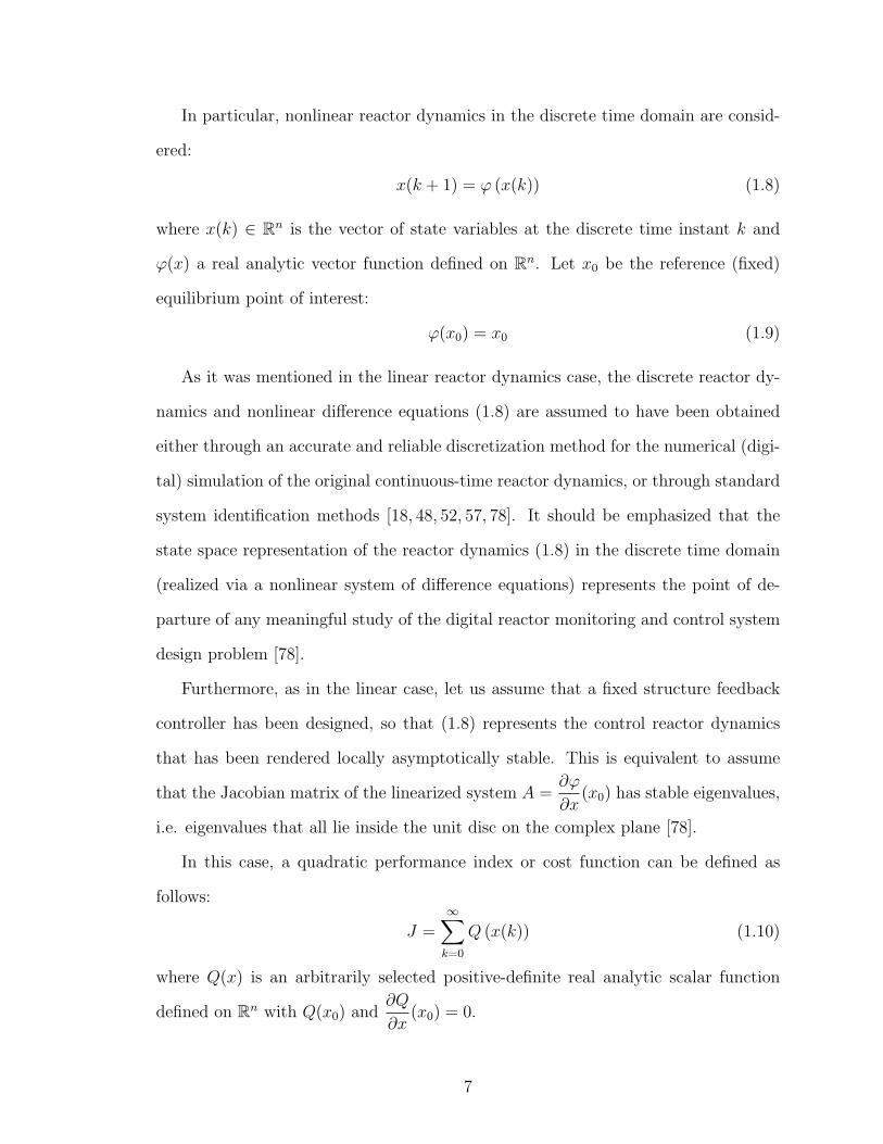
Figure 1.2: Optimal values of p2 as a function of the size of the step change in theset point

obtained with a weight coefficient ρ = 10−5. Please notice that the step size is a

measure of how drastic the disturbance effect has been, driving the system far from

the desired final equilibrium state.

As suggested by Figures 1.1 and 1.2, the optimal values of the regulator param-

eters p1 and p2 are highly dependent on the step size. This is of course intuitively

expected due to the nonlinear nature of the system under study. An additional piece

of information provided by these figures, is that fast convergence is attained, as the

order of series truncation N increases. In this particular case study, an order of

truncation N = 4 is enough for a satisfactory approximation.

Figures 1.3 and 1.4 show the optimal responses obtained with different values of

the weight coefficient ρ. As expected, when the weight coefficient ρ attains small

values the system’s response is very fast, but at the expense of unrealistic values

of the dilution rate. Indeed, as we lower the value of ρ, we tend not to drastically

penalize the control effort needed for reactor regulation, the regulator becomes more

20

Figure 1.3: Optimal output responses to a step change in the set point from 1.2gmol/lto 1.05gmol/l with different weight coefficient

aggressive, the reactor response that it induces faster, but the values of the input

variable that are generated may become physically unrealizable. The opposite effect

is naturally observed for larger values of the weight coefficient ρ. In this case, a large

control effort u is severely penalized, the regulator becomes less aggressive enforcing a

dynamically more sluggish response and reversion to the desired reference equilibrium

state.

Finally, Figures 1.5 and 1.6 illustrate how the method described in Section 2 is

used to obtain stability region estimates. This is a very useful feature of the proposed

method, because it also equips us with the capacity to assess the reactor’s stability

characteristics under the optimal regulator parameters. In particular, stability region

estimates were obtained by considering the largest contour curve of the function V (x)

which is tangent to the ∆V (N)(x) = 0 curve, and wholly contained in the region where

∆V (N)(x) < 0 [75,80].

21

Figure 1.4: Optimal intput responses to a step change in the set point from 1.2gmol/lto 1.05gmol/l with different weight coefficient

1.5 Concluding Remarks

A systematic methodology was presented that responds to the need of optimiz-

ing the digitally controlled reactor dynamics. The method is based on the explicit

calculation of the value of a physically meaningful performance index through the so-

lution of a Zubov-like functional equation. A static optimization scheme provides the

optimal reactor regulator parameters through the minimization of the parameterized

performance index. The properties of the solution of the Zubov-like functional equa-

tion allow the derivation of stability region estimates associated with the controlled

reactor dynamics. Finally, the proposed method was illustrated in a nonlinear chem-

ical reactor example and its satisfactory performance demonstrated via simulation

studies.

22

Figure 1.5: Geometric interpretation of the method for estimating the stability regionwith N = 4, p1 = 46.4l2/h ·mol, p2 = 57.3l2/h ·mol

Figure 1.6: Stability region estimates for N = 2 and N = 4 with p1 = 46.4l2/h ·mol,p2 = 57.3l2/h ·mol

23

CHAPTER 2A Model-Based Characterization of the

Long Term Asymptotic Behavior of

Nonlinear Discrete-Time Processes

2.1 Introduction

The chemical engineering literature is dominated by physical and (bio)chemical

processes that exhibit nonlinear behavior and are typically modeled by systems of non-

linear ordinary (ODEs) or partial differential equations (PDE) in the continuous-time

domain , or systems of nonlinear difference equations (DEs) in the discrete-time do-

main [8,18,79,82]. Furthermore, accompanying the growing computational capacities,

efficient and accurate discrete-time dynamic process modeling techniques have been

developed, allowing the digital simulation, analysis and characterization of complex

process dynamic behavior to be performed in a thorough manner. Particularly, the

development of efficient discretization techniques, applied to a system of ODEs/PDEs

or various process identification methods in the continuous-time domain, can provide

us with discrete-time dynamic models characterized by a high degree of fidelity, al-

lowing insightful theoretical and computational investigations on the process dynamic

24

behavior. Nevertheless, despite the fact that the dynamic analysis of linear processes

can be performed with rigor [8,27,82], the task remains very challenging for nonlinear

processes. Particular efforts in nonlinear dynamic analysis have been concentrated on

reducing the dimensionality of the original problem [3, 11, 21, 33, 34, 45, 54, 77, 84, 99].

Within the above framework, the restriction of the system dynamics on an invari-

ant manifold results in a reduced-order dynamic model, and essentially determines

the long-term asymptotic behavior, since the original transition or approach to the

manifold can be proven to be rather fast under certain conditions. Some representa-

tive recent applications of invariant manifold theory to chemical reaction systems for

model-reduction purposes can be found in various publications [6,43,70,72,83,97,101].

Furthermore, the study of invariant manifolds has been historically conducted in con-

nection with the existence problem of a stable, unstable or center manifold, stability,

as well as bifurcation analysis [99]. One should however notice that the stable and

center manifold theory presupposes the successful transformation of the original non-

linear dynamical system into one whose Jacobian matrix of the linearized system

around the equilibrium point of interest is in Jordan canonical form, and the corre-

sponding stable, unstable and center eigenmodes appear as decoupled (the state space

of interest being the direct sum of the stable, unstable and center eigenspaces) [99].

The later requirement, while always achievable through a coordinate transformation,

may result in a computationally demanding numerical problem particularly for higher

order systems, such as the ones obtained from discretization or modal decomposition

techniques applied to distributed parameter systems [18]. Following the ideas used

for the standard stable and center manifold theory, conceptual and technical exten-

sions have been developed in the case of singularly perturbed systems, where the

classification of the corresponding invariant manifolds as slow and fast is a natural

consequence of the two-time scale separation property [30,64]. Moreover, a conceptu-

ally similar geometric notion of a positively invariant finite-dimensional manifold was

25

introduced in the study of the dynamic model reduction problem for parabolic PDE

systems under the name of inertial manifold [18]. One should notice that unlike the

existence theorems available for the standard stable and center manifold theory [99],

inertial manifolds were proven to exist only for certain classes of parabolic PDEs (on

a case-by-case basis). However, there are systematic techniques available for com-

puting, up to a certain degree of accuracy, approximations of the so-called manifold

equation [18]. Finally, research results on symmetry-induced generalized invariants

for distributed parameter systems were also reported in [81].

A systematic approach is proposed in the present research study [58], to rigor-

ously address the problem of quantitatively characterizing the long-term dynamic

behavior of non-linear discrete-time processes using the notion of invariant manifold.

The problem under consideration is naturally formulated as a system of nonlinear

functional equations (NFEs), and a set of rather general solvability conditions can be

derived. This set of conditions guarantees the existence and uniqueness of a locally

analytic solution, which is then proven to represent a locally analytic invariant man-

ifold of the nonlinear discrete-time process dynamincs considered. However, within

the proposed framework of analysis, the formulation of the problem of interest does

not require the special structure of the Jacobian eigenspace of the linearized sys-

tem associated with the classical stable and center manifold theory, thus effectively

overcoming the associated problems of computing the requisite transformation into

the Jordan canonical form with the explicit decoupling of the stable, unstable and

center eigenspaces, as well as the numerical solution to the associated eigenstructure

problem [99]. Furthermore, the local analyticity property of the invariant manifold

map enables the development of a series solution method, which can be easily im-

plemented using MAPLE. Under a certain set of conditions, it can be shown that

the invariant manifold computed attracts all system trajectories, and therefore, the

asymptotic process response and long-term dynamic behavior are calculated through

26

the restriction of the discrete-time process dynamics on the invariant manifold.

The present chapter is organized as follows: Section 2.2 contains some mathemat-

ical preliminaries that are necessary for the ensuing theoretical developments. The

chapter’s main results are presented in Section 2.3, accompanied by remarks and

comments on their potential use for process performance monitoring purposes. An

illustrative case study of an enzymatic bioreactor is presented in Section 2.4, followed

by a few concluding remarks in Section 2.5.

2.2 Mathematical preliminaries

A nonlinear discrete-time dynamic process model is considered with a state space

representation of the following form:

x(k + 1) = F (x(k), w(k)) (2.1)

which is driven by the states of an exogenous nonlinear discrete-time autonomous

dynamical system:

w(k + 1) = G (w(k)) (2.2)

where k ∈ N is the discrete-time index and N the set of positive integers, x ∈ Un ⊂ Rn

is the process state vector, w ∈ Um ⊂ Rm is the state vector associated with dynamics

(2.2), and Un, Um are open subsets of the Euclidean spaces Rn and Rm respectively.

Notice that the above dynamic process description in the discrete-time domain may

represent a process whose dynamics (2.1) is driven by:

(i) the input/disturbance dynamics (2.2), where input or disturbance changes are

modeled and generated as outputs of the exogenous dynamical system (2.2), or

(ii) a time-varying process parameter vector w(k) that follows dynamics (2.2) and

models phenomena such as catalyst deactivation, enzymatic thermal deactiva-

tion, heat-transfer coefficient changes, time-varying (bio)chemical kinetic pa-

rameters, etc., or

27

(iii) the autonomous dynamics of an upstream process modeled by (2.2), in which

case, a cascade connection of the two nonlinear processes results in the ”block-

triangular” structure (2.1)-(2.2).

As stated in the introductory Section 2.1 ,it is also assumed that the discrete-time

dynamic process model (2.1)-(2.2) is obtained:

(a) either through the deployment of efficient and accurate discretization methods

for the original continuous time process (modeled by a system of nonlinear

ordinary (ODEs) or partial differential equations (PDEs) that mathematically

reflect the underlying fundamental phenomena) or

(b) through direct identification methods.

It is also assumed that the F (x, w) and G(w) maps of the discrete-time dynamics

(2.1)-(2.2) are real-analytic vectors functions defined on Un×Um and Um respectively.

Without loss of generality, let the origin x0 = 0 be an equilibrium point of (2.1):

F (0, 0) = 0, that corresponds to w0 = 0 with G(0) = 0. The following assumption is

also made:

Assumption 2.1.

Matrix A:

A =∂G

∂w(0) (2.3)

has non-zero eigenvalues ki, (i = 1, ...,m) that all lie inside or outside the unit disk

(Poincare domain [3]). This assumption implies that the w-dynamics is either locally

asymptotically stable or unstable, and that the G(w) map is locally invertible around

w0 = 0.

28

The original nonlinear discrete-time dynamic process model (2.1)-(2.2) may there-

fore be rewritten as follows:

x(k + 1) = Bx(k) + Cw(k) + f (x(k), w(k))

w(k + 1) = Aw(k) + g (w(k)) (2.4)

where B,C are constant matrices with appropriate dimensions, and f(x, w), g(w) are

real analytic functions of x and w with f(0, 0) =g(0), and∂f

∂x(0, 0) =

∂f

∂w(0, 0) =

∂g

∂w(0) = 0.

The following definitions are essential for the ensuing developments.

Definition 2.1.

A set S ∈ Rm+n is said to be invariant under the flow of the nonlinear discrete-time

dynamics 2.4 if for each (x0, w0) ∈ S, the orbit Ω = (x(k), w(k)) , k ∈ N satisfying

((x(k = 0), w(k = 0)) = (x0, w0), is such that (x(k), w(k)) ∈ S for all k ∈ N [99].

Definition 2.2.

An invariant set S ⊂ Rm+n passing through the origin (x0, w0) = (0, 0) is said

to be an locally analytic invariant manifold of (2.4) , if S has the local topological

structure of an analytic manifold around the origin [99].

2.3 Main results

Together with the original nonlinear discrete-time input-driven dynamic process

model (2.4) an associated system of nonlinear first-order functional equation (NFEs)

is also considered:

π(Aw + gw) = Bπ(w) + Cw + f(π(w), w)

π(0) = 0(2.5)

where π : Rm → Rn is the unknown vector function of 2.5.

The following technical lemma reported in [55] is necessary.

29

Lemma 2.1.

Suppose that for the nonlinear discrete-time dynamic process model (2.1)-(2.2)

Assumption 2.1 holds true.

Consider the system of NFEs (2.5) and assume the eigenvalues ki, (i = 1, ...,m)

of matrix A =∂G

∂w(0) are not related to the eigenvalues λi, (i = 1, ..., n) of matrix

B =∂F

∂x(0, 0) through any equation of the following type:

m∏i=1

kdii = λj (2.6)

(j = 1, ..., n), where all the di’s are nonnegative integers satisfying the condition:

m∑i=1

di > 0 (2.7)

Then, the associated system of NFEs (2.5) admits a unique locally analytic solu-

tion π(w) in a neighborhood of w = 0

Remark 2.1. Let us now consider the linear case where G(w) = Aw and F (x, w) =

Bx + Cw, with A, B, C being constant matrices with appropriate dimensions. The

unique solution to the system of functional equations (2.5) is given by: π = Πw where

Π is the solution of the Lyapunov-Sylvester matrix equation:

ΠA−BΠ = C (2.8)

It is known that the above linear matrix equation (2.8) admits a unique solution

Π as long as the eigenspectra of matrices A, B are disjoint [38]. Notice, that the latter

is guaranteed by the assumptions of Lemma 2.1, and, therefore, the linear result can

be naturally reproduced.

We are now in a position to present this chapter’s main results.

Theorem 2.1.

30

Suppose that for the nonlinear discrete-time dynamic process model (2.1)-(2.2)

Assumption 2.1 holds true, as well as the assumptions of Lemma 2.1.

Then, there exists a neighborhood V ⊂ Rm of w0 = 0, and a unique locally analytic

mapping π : V → Rn such that:

S = (x, w ∈ Rn × V : x = π(w), π(0) = 0 (2.9)

is an analytic local invariant manifold of (2.1)-(2.2) (in the sense of Definition 2.2)

that passes through the origin (x0, w0) = (0, 0), where π(w) is the unique solution of

the associated system of NFEs (2.5).

Proof of Theorem 2.1. For the graph of the mapping x = π(w) to be a local invariant

manifold that passes through the origin (x0, w0) = (0, 0), it has to satisfy the following

system of invariance NFEs:

π(Aw + g(w)) = Bπ(w) + Cw + f(π(w), w)

x(0) = 0(2.10)

The above equation can be easily deduced by applying the one-step forward in

time-operator on x = π(w) and along an arbitrary solution curve (x(k), w(k)) of

(2.1) and (2.2) which belongs to the manifold of interest, i.e. identically satisfies:

x(k) = π(w(k)).

The above system of invariance NFEs (2.10) is exactly the system of NFEs (2.5)

associated with the original discrete-time dynamics and the maps F (x, w) and G(w).

Under the assumptions stated, the above system of NFEs (2.10) admits a unique and

locally analytic solution in a neighborhood V ⊂ Rm of w0 = 0 due to Lemma 2.1.

Therefore:

S = (x, w ∈ Rn × V : x = π(w), π(0) = 0 (2.11)

is indeed an analytic local invariant manifold of (2.1) and (2.2).

Remark 2.2. The invariant manifold x = π(w) of Theorem 2.1, that is computed

through the solution of the associated system of NFEs (2.5), may coincide with the

31

system’s stable or unstable manifold under certain conditions. For a more thorough

discussion on this matter, the interested reader is refered to [55].

Remark 2.3. For practical reasons, one must provide a solution scheme for the

system of invariance NFEs (2.5).

Notice that F (x, w), G(w) and π(w) are locally analytic, and therefore, the pro-

posed method suggests their expansion in Taylor series, followed by a procedure that

equates the same order Taylor coefficients of both sides of (2.5). This procedure leads

to recursion formulas, through which one can calculate the Nth-order Taylor coeffi-

cients of the unknown solution x = π(w), given the Taylor coefficients of x = π(w)

up to order N − 1 by solving a system of linear equations. In the derivation of the

recursion formulas, it is convenient to use the following tensorial notation:

a. The entries of a constant matrix A are represented as aji , where the subscript i

refers to the corresponding row and the superscript j refers to the corresponding

column of the matrix.

b. The partial derivatives of the µ-th component Fµ(x, w) of the vector function

F (x, w) evaluated at (x, w) = (x0, w0) are denoted as follows:

F iµ =

∂Fµ

∂xi

(0, 0)

F ijµ =

∂2Fµ

∂xi∂xj

(0, 0)

F ijkµ =

∂3Fµ

∂xi∂xj∂xk

(0, 0), etc...

where i, j, k=1, ..., n.

c. The partial derivatives of the µ-th component Fµ(x, w) of the vector function

F (x, w) with respect to the variables w evaluated at (x, w) = (0, 0) are denoted

as follows: F iµ =

∂iFµ

∂wi(0, 0), etc.

d. The standard summation convention where repeated upper and lower tensorial

indices are summed up.

32

Under the above notation, the l-th component pil(w) of the unknown solution

π(w) can be expanded in a multivariate Taylor series as follows:

πl(w) =1

1!πi1

l wi1 +1

2!πi1i2

l wi1wi2 + ...

+1

N !πi1i2...iN

l wi1wi2 ...wiN + ... (2.12)

and similarly for F (x, w) and G(w). Inserting the Taylor expansions of π(w),F (x, w)

and G(w) into (2.5) and matching the Taylor coefficients of the same order, the

following relation for the Nth order can be obtained:

N∑L=1

∑0≤m1≤...≤mL

πj1...jL

l Gm1j1

...GmLjL

= F µl πi1...iN

µ + F i1...iNl + f i1...iN

l (πi1...iN−1) (2.13)

where i1, ..., iN = 1, ...,m, l = 1, ..., n,∑L

j=1 mj = N and f i1...iNl (πi1...iN−1) is a func-

tion of Taylor coefficients of the unknown solution π(w) calculated in the previous

recursive steps. Note that the second summation symbol in (2.13) suggests summing

up the relevant quantities over the N !m1!...mL!

possible combinations to assign the N

indices (i1, ...iN) as upper indices to the L positions Gj1 ...GjL, with m1 of them being

put in the first position, m2 of them in the second position, etc. (∑L

j=1 mj = N).

Furthermore, notice that equations (2.13) represent a set of linear algebraic equations

in the unknown coefficients πi1,...iNµ . Finally, a MAPLE code similar to the code found

in Appendix A has been developed to automatically compute the Taylor coefficients

of the unknown solution x = π(w) of NFEs (2.5).

Theorem 2.2. Let matrix B have stable eigenvalues (|λi| < 1, i = 1, ...n) and all

assumptions of Theorem 2.1 hold true. Furthermore, let S defined in equation (2.9)

be an invariant manifold of (2.1)-(2.2), where π(w) is the solution to the associated

system of invariance NFEs (2.5) and (x(k), w(k)) a solution curve of (2.1)-(2.2).

33

There exists a neighborhood U0 of the origin (x0, w0) = (0, 0) and a real number

M ∈ (0, 1) such that, if (x(0), w(0) ∈ U0), then:

||x(k)− π((w(k))||2 ≤ (M)k||x(0)− π(w(0))||2 (2.14)

Proof of Theorem 2.2. Denote by z the ”off-manifold” coordinate:

z(k) = x(k)− π(w(k)) (2.15)

whose dynamics is described by:

z(k + 1) = B(z(k) + π(w(k))) + Cw(k) + f(z(k) + π(w(k)), w(k))

−Bπ(w(k))− Cw(k)− f(π(w(k)), w(k))

= Bz(k) + N(z(k), w(k)) (2.16)

where: N(z, w) = f(z +π(w), w)− f(π(w), w). Notice that N(z, w) is a real analytic

vector function with: N(0, 0) = 0 and no linear terms in z: ∂N∂z

(0, 0) = 0. Conse-

quently: ||N(z,w)||2||z||2 → 0 as ||z‖2 → 0, and thus, for an arbitrary constant L > 0 there

exist positive ρ1, ρ2, such that in the domain: ‖z‖2 < ρ1, ‖w‖2 < ρ2 the following

inequality holds:

‖N(z, w)‖2 < L‖z‖2 (2.17)

Furthermore, since matrix B has all its eigenvalues with modulus less than one,

there exist positive constants β ∈ (0, 1) and γ such that [11,27]:

‖(B)ky‖2 ≤ γ(β)k‖y‖2 (2.18)

for all y ∈ Rn.

From equation (2.16), one obtains [27]:

z(k) = (B)kz(0) +k−1∑j=0

(B)k−j−1N(z(j), w(j)) (2.19)

and therefore:

‖z(k)‖2 ≤ γ(β)k‖z(0)‖2 +k−1∑j=0

γL(β)k−j−1‖z(j)‖2 (2.20)

34

or:

(β)−k‖z(k)‖2 ≤ γ

(‖z(0)‖2 +

k−1∑j=0

L(β)−j−1‖z(j)‖2

(2.21)

Applying Gronwall-Bellman’s inequality [27], it can be deduced that:

(β)−k‖z(k)‖2 ≤ ‖z(0)‖2

k−1∏j=0

(1 + γL(β)−1)

⇒ (β)−k‖z(k)‖2 ≤ ‖z(0)‖2(β)−k(β + Lγ)k

⇒ ‖z(k)‖2 ≤ (M)k‖z(0)‖2

⇒ ‖x(k)− π(w(k))‖2 ≤ (M)k‖x(0)− π((w(0))‖2 (2.22)

where M = β + Lγ. Since L can be made arbitrarily small, let is choose L < 1−βγ

so

that 0 < M < 1, and the proof is complete.

Theorem 2.2 states that, as time tends to infinity (asymptotically), any trajectory

of the overall system (2.1)-(2.2) starting at a point sufficiently close to the origin

converges to a trajectory that lies entirely on the invariant manifold S. Therefore,

the long-term asymptotic response of the nonlinear process (2.1) in the presence of

the w-dynamics (2.2) is given by:

x(k) ≈k→∞

π(w(k)) (2.23)

where π(k) is the solution of the associated system of invariance NFEs (2.5). Equiva-

lently, under the assumption of Theorem 2.2, the invariant manifold S (2.9) computed

through the associated system of NFEs (2.5) is rendered locally ”attractive” [11], and

the restriction of the process dynamics on the aforementioned manifold (often termed

as the ”slow dynamics” or the ”dynamics on the slow manifold”) embedded in state

space determines the long-term asymptotic behavior of the process [99]:

w(k + 1) = G(w(k))

x(k) ≈k→∞

π(w(k))(2.24)

35

Remark 2.4. The seminal work presented in [37, 93, 98] on chemical reaction in-

variants/variants is fundamentally different in scope and technically from the pro-

posed one. In their respective framework of analysis, the above publications aim

at identifying classes of linear variable transformations that reflect the basic under-

lying conservation laws (for atoms, charge and energy) dictated by stoichiometry,

kinetics, thermodynamics and possibly reactor operating conditions (linear invariant

subspaces). Therefore, the above approaches identify all constraints that the process

dynamics ought to obey and typically lead to the smallest number of independent

transformed variables whose dynamic evolution suffices for a unique characteriza-

tion of the process dynamic state. The proposed work presupposes that the state

space representation (2.1) and (2.2) is already realized by the smallest number of

independent state variables (for simple systems, this task can be easily carried out;

the aforementioned approaches focus primarily on complex chemical reaction systems

with numerous reactions and species for which the task is not trivial), and aims at

identifying the nonlinear map of an attracting manifold (in certain cases the stable

manifold itself [55]), on the basis of which the slow process dynamics (once the fast

transients die out) can be explicitly characterized. The two approaches could conceiv-

ably be used in tandem for model reduction purposes of complex chemical reaction

systems.

Remark 2.5. The possibility of integrating the proposed approach into a nonlinear

MPC synthesis framework certainly deserves further examination and traces a mean-

ingful line of future research work. On an intuitive level, it is expected that nonlinear

controller design based on the methodological principles of MPC for the process dy-

namics evolving on the stable slow manifold can be considerably simplified, and the

associated on-line optimization problem become less computationally demanding due

to the lower dimensionality of the problem under consideration.

36

2.3.1 Special Case: The Long-Term Dynamic Behavior of Linear Discrete-Time Processes

Let us now consider the special case of a linear (or linearized around a reference

steady state (x0, w0)) discrete-time dynamic process model:

x(k + 1) = Bx(k) + Cw(k) (2.25)

where x ∈ Rn is the vector of process state variables, and for the sake of simplicity, let

w ∈ R be a time-varying scalar process parameter following the first-order dynamics:

w(k + 1) = aw(k) (2.26)

with B,C being constant matrices with appropriate dimensions and |a| < 1 (sta-

bility assumption for the w-dynamics). Notice that one may envision a case where

a chemical reaction system with z being the composition vector (in deviation form

from the reference steady state conditions), and w the catalyst activity (in devia-

tion form as well) corresponding to a specific deactivation mechanism, is modeled by

(2.25)-(2.26) [32]. In this representative case, the objective is to calculate the long-

term asymptotic behavior of the chemical reaction system (2.25) in the presence of

catalyst deactivation (2.26), and therefore, to investigate the possibility of catalyst

replacement if conversion or selectivity are affected in an adverse manner.

It is assumed that the eigenspectrum of the process characteristic matrix B is

comprised of eigenvalues λi with λi < 1, i = 1, ..., n, and therefore the discrete-time

process (2.25) is assumed to be a stable one. Notice, that in the case of an unstable

process, one could assume that a stabilizing controller has been already synthetized to

ensure closed-loop stability, and therefore, the previous stability assumption should

not be viewed as a restrictive one within the context of the present study. Fur-

thermore, it is assumed that the time-constant associated with the catalyst activity

w-dynamics is larger compared to the dominant process time-constant:

|a| >> ρ (2.27)

37

where ρ = maxi |λi|, (i = 1, ..., n) is the spectral radius of the process characteris-

tic matrix B. Within the current context, this assumption appears to be valid and

reasonable for chemical reaction systems where catalyst deactivation by poisoning

occurs [32]. One may now explicitly calculate the long-term asymptotic process re-

sponse in the presence of catalyst deactivation (2.26) through a direct computation

of the solution x(k) of the system of linear difference equations (2.25) and (2.26) [27]:

x(k) = Bkx(0) +k−1∑i=0

Bk−i−1Caiw(0)

= Bkx(0)− w(0)akI −Bk

(B − aI)−1C (2.28)

where the following matrix identity was used:

k−1∑j=0

Bk−j−1aj =Bk − akI

(B − aI)−1 (2.29)

Under assumption (2.27), it can be easily inferred that the longterm asymptotic

response of the linear discrete-time process (2.25) in the presence of catalyst deacti-

vation (2.26) is given by:

x(k) ≈k→∞

−w(0)(B − aI)−1Cak (2.30)

It should be pointed out that the same expression for the long-term asymptotic

process response can be derived by following the proposed approach which is based on

the explicit construction of the invariant manifold S (2.9). Indeed, in the linear case

(2.25) and (2.26), the associated system of invariance NFEs (2.5) takes the following

form:

π(aw) = Bπ(w) + Cw

π(0) = 0(2.31)

Under the assumptions of Theorem 2.1, the above system of NFEs admits a unique

solution:

π(w) = Πw (2.32)

38

where Π is the unique solution that satisfies the following Lyapunov matrix equation:

ΠaI −BΠ = C (2.33)

It is easy to show that (2.33) admits the following solution:

Π = −(B − aI)−1C (2.34)

where (B−aI) is indeed an invertible matrix since a does not belong to the eigenspec-

trum of the process characteristic matrix B, which is guaranteed by Lemma 2.1 and

Theorem 2.1. According to Theorem 2.2, the invariant manifold x = Πw is locally

attractive, and the long-term asymptotic behavior of the chemical reaction system

(2.25) in the presence of catalyst deactivation (2.26) is given by:

x(k) ≈k→∞

Πw(k) = −w(0)(B − aI)−1Cak (2.35)

The above expression was derived on the basis of the invariant manifold construc-

tion of the proposed approach, and it coincides with the one (Eq. (2.30)) obtained

through a direct calculation of the solution of the discrete-time linear process dynamic

equations (2.25) and (2.26). Notice that the proposed approach naturally reproduces

the results offered by linear analysis, and it can be therefore viewed as its nonlinear

analogue.

2.4 Illustrative example

Immobilized cell and enzyme bioreactors are now widely used in a variety of in-

teresting applications. In these systems, the short-term behavior of the bioreactor is

dependent upon the nonlinear kinetics of the immobilized enzymes or cells participat-

ing in the reactions. However, the long-term behavior of the bioreactors depends upon

the stability of the immobilized enzymes or the viability of the immobilized cells. The

short-term behavior of these systems is important in determining the conversion of a

39

nutraceutical or degradation of a toxin, for example, parameters that define the per-

formance of the bioreactor. The long-term behavior of the bioreactor will determine

when the enzyme or cell catalyst needs to be replaced in order to maintain conversions

at acceptable levels. Therefore, accurately estimating when bioreactor performance

declines below acceptable levels has important consequences for the profitability of a

process or the health of a patient. Actual kinetic data on enzyme performance and

enzyme degradation are considered in the present study for an immobilized enzyme

bioreactor that is used for the production of food grade linoleic acid from corn oil [88].

In the case study considered, we assume that the enzymatic bioreactor behaves as

an ideal continuous stirred tank reactor (CSTR). It is also assumed that the enzyme

involved converts substrate into product, in this case corn oil into linoleic acid, via

a pingpong bi-mechanism, as reported in [88]. Under a set of standard assumptions,

the following nonlinear dynamic process model can be developed:

dS

dt= f (1)(S, E) =

k1ES

1− k2S+

v0

V(S0 − S)

dE

dt= g(1)(E) = −kd1E

(2.36)

Parameter ValueS0 3.4MS(t = 0) 3ME(t = 0) 3gV 50mlv0 100ml/hk1 8.2× 10−2h−1g−1

k2 5.9× 10−1M−1

kd1 3.4× 10−3h−1

Table 2: Kinetic and bioreactor parameter values

The above dynamic equations describe the change in substrate concentration in

the reactor as a function of time, and the degradation of activity of the enzyme. S, S0

and E represent the concentrations of substrate, substrate in the feed stream and

enzyme, respectively. k1 and k2 represent kinetic parameters describing the rate of the

40

enzymatic reaction and kd1 is a kinetic parameter describing the rate of deactivation of

the enzyme. v0 is the flow rate of the substrate and V is the reactor volume. In Table

2, kinetic parameters used in the example, as well as initial substrate and enzyme

concentrations, are provided. It is worth mentioning that under these parameter

values, the above bioreactor dynamics is characterized by a latent two-time scale

multiplicity attributed to the slow degradation of the enzyme when compared to the

much faster bioprocess dynamics. Using a time-discretization step: δ = 0.01h, which

is smaller than the dominant process time-constant, Euler’s discretization method

was applied in order to obtain a quite accurate discrete-time dynamic process model

(sampled-data representation of (2.36)):

S(k + 1) = F (1)(S(k), E(k)) = S(k) + f (1)(S(k), E(k))δ

E(k + 1) = G(1)(E(k)) = E(k) + g(1)(E(k))δ(2.37)

In order to conform to the theory presented in previous sections, the following

set of deviation variables relative to the equilibrium point (S0, E0) = (3.4, 0) is intro-

duced:

x = S − S0

w = E − E0(2.38)

Let us also denote: F (1)(x, w) = F (1)(x + S0, w + E0), G(1)(w) = G(1)(, w + E0).

Notice that for the bioreactor model (2.37), all conditions of Theorems 2.1 and 2.2

are satisfied. Therefore, there exists a unique and locally analytic invariant manifold:

x = π(w), with π(w) being the solution of the following nonlinear functional equation:

π(G(1)(w)) = F (1)(π(w), w)

π(0) = 0(2.39)

A series solution of the above functional equation is sought around the origin. The

Taylor coefficients of the unknown solution x = π(w) can be automatically computed

by using a simple MAPLE code. A finite-order series truncation N is considered

leading to a Taylor polynomial approximation u = π[N ](w) of the actual solution

41

Figure 2.1: Phaseportrait of the bioreactor dynamics slow manifold (N = 5).

of the invariance nonlinear functional equation (2.39). In particular, with the aid of

the aforementioned MAPLE code up to a 10th-order series truncation was considered:

N = 1, ..., 10. Figs. 2.1 and 2.2 represent the phaseportrait of the bioreactor dynamics

along with the actual slow invariant manifold (depicted through the solid line) and the

one obtained through the solution of the invariance functional equation (2.39) for N =

5 and 10, respectively (depicted through the dotted line). It should be first pointed out

that the underlying two-time scale multiplicity manifests itself quite explicitly and the

familiar dynamic pattern naturally emerges [64]: the transition of the system from the

initial state to the slow manifold is depicted through the vertical constant-E lines since

the enzymatic concentration remains practically unchanged due to the much slower

enzymatic dynamics, while the substrate concentration changes rather rapidly until

the system reaches the slow manifold, upon which the bioreactor dynamics is bound

to evolve (for large times). Please notice the satisfactory approximation of the actual

slow invariant manifold by the proposed method in the case of N = 5, and the almost

indistinguishable curves in the N = 10 case. As intuitively expected and as a result

42

Figure 2.2: Phaseportrait of the bioreactor dynamics slow manifold (N = 10).

of the uniform convergence of the series solution of (2.39), numerical convergence

to the actual slow invariant manifold can be satisfactorily demonstrated. Both the

actual dynamic response of the bioreactor was computed by simulating the full process

model (2.37), as well as the long-term asymptotic behavior of the bioreactor by using

the proposed method and Eq. (2.24) with N = 10 and u = π[10](w), a 10th-order

Taylor polynomial approximation of the actual solution of the invariance functional

equation (2.39). As it can be seen in Fig. 2.3, the estimated substrate concentration

profile (dotted line) at the outlet of the reactor obtained through the proposed method

becomes indistinguishable from the actual substrate concentration profile (solid line)

at times larger than 100h, which is less than the approximate half-life of the decaying

enzyme. Fig. 2.4 shows the actual conversion profile (solid line) in the bioreactor

as well as the conversion estimated (dotted line) from the asymptotic behavior of

the bioreactor as characterized through the proposed method. Please notice that the

proposed method accurately approximates the actual conversion profile, and therefore

allows the satisfactory monitoring of the actual bioprocess performance, at times much

43

Figure 2.3: Comparison between the actual and estimated substrate concentrationprofiles (N = 10).

shorter than the half-life of the decaying enzyme.

2.5 Concluding remarks

A new approach to the problem of computing and quantitatively characterizing

the long-term dynamic behavior of nonlinear discrete-time processes was presented.

The formulation of the problem of interest was conveniently realized through a system

of nonlinear functional equations for which a rather general set of conditions for the

existence and uniqueness of a locally analytic solution was derived. The solution to

the aforementioned system of NFEs was then shown to represent a locally analytic

invariant manifold of the nonlinear discrete-time dynamic process model considered.

The local analyticity property of the invariant manifold enabled the development of

a series solution method, which can be easily implemented using a simple MAPLE

code. Under a certain set of conditions, it was also shown that the invariant mani-

fold computed attracts all system trajectories, and therefore, the asymptotic process

response and long-term dynamic behavior can be explicitly determined through the

44

Figure 2.4: Comparison between the actual and estimated substrate conversion pro-files (N = 10).

restriction of the discrete-time process dynamics on the invariant manifold.

45

CHAPTER 3Nonlinear Observer Design for Process

Monitoring in the Presence of Time-Scale

Multiplicity

3.1 Introduction

The problem of the development of operationally flexible and reliable methods

to accurately reconstruct the unmeasurable process state variables, as well as other

key quantities associated with process safety and/or product quality, is of central

importance in process control, monitoring and diagnostics [24, 92]. Indeed, techni-

cal limitations and cost-related considerations that affect segments of current sensor

technology, as well as inherent physical limitations associated with the measurement

of certain physical and/or chemical quantities, necessitate and motivate the devel-

opment of methods that allow the accurate estimation of the above unmeasurable

quantities [24, 92]. A widely followed strategy to accomplish this objective relies

on the design of model-based state observers that make explicit use of the available

process measurements and are capable of providing accurate estimates for the unmea-

surable process state variables [24,92]. For linear processes, both the popular Kalman

46

filter [40] and its deterministic analogue known as the Luenberger observer [73], form

the basis of a comprehensive and practically intuitive framework that adequately

addresses the linear state estimation problem. However, the recognition that the

majority of physical and/or chemical processes exhibit nonlinear behavior and the

occasional difficulties encountered when linear observers are designed on the basis of

linearized process models characterized of local validity [24, 92], induced a wave of

research efforts aiming at developing the requisite nonlinear observer design methods

that could directly cope with process nonlinearities. As a result, a number of notable

nonlinear observer design frameworks emerged, where various methodological objec-

tives were pursued and perspectives offered, as well as different aspects of the under-

lying state estimation problem emphasized [1,4,9,19,22,23,29,39,44,65–69,71,91,96].

However, all the above approaches presuppose the availability of a dynamic process

model that does not exhibit time-scale multiplicity (a process dynamic response char-

acteristic that naturally arises in a multitude of applications), and most importantly,

the sensor dynamics is not integrated into their respective observer design frame-

works, and thus its impact on the viability and performance of the proposed observer

remains inevitably unaddressed. Please notice, that for processes exhibiting fast and

slow dynamic modes (such as instrumented processes where there is a latent time-

scale separation property that distinguishes the fast sensor dynamics from the slow

process dynamics, as well as reactor networks and classes of bioprocesses that exhibit

inherent time-scale multiplicity [14,16,70], the state estimation problem becomes not

only theoretically challenging due to the multiple timescales, but practically an in-

triguing and important one [13, 62, 74]). Indeed, one could in principle realize the

design of the nonlinear observer through the restriction of the process dynamics on

the slow manifold (the reduced-order process dynamic model), and thus capitalizing

on all the computational and analytical advantages that the lower-dimensionality of

47

the problem of interest brings, followed by a detailed, rigorous and insightful anal-

ysis on the impact of the ignored fast dynamics (otherwise known as parasitics) on

the convergence properties of the reduced-order observer [62, 74]. It should be em-

phasized, that the design of nonlinear observers based on the reduced-order process

dynamic model on the slow manifold is motivated by the fact that model-based es-

timation problems for systems/processes exhibiting time-scale multiplicity, and thus

stiff dynamics, may lead to ill-conditioned observer gains and potentially undermine

the convergence properties of an observer designed for the full-order singularly per-

turbed system (3.1) [16, 70]. Please notice that the aforementioned problem has

been thoroughly studied for linear systems [49], and within a singular perturbation

framework of analysis, pursued by a few researchers on the nonlinear front as well.

In particular, high-gain [15, 26, 62, 74, 94] and sliding-mode observers [46] have been

designed for special classes of nonlinear systems, that explicitly take into account

the underlying time-scale separation property of the system under consideration, and

nicely embedded it into their respective frameworks of analysis and design.

The present work [59], while adopting a singular perturbation framework of anal-

ysis, aims at developing a generic and systematic nonlinear observer design method

for fast/slow systems, as well as overcoming some of the restrictions associated with

the above approaches by following a methodologically and technically different path.

In particular, a nonlinear observer is designed on the basis of the reduced order pro-

cess dynamics evolving on the slow manifold, and the effect of the unmodeled fast

component (which may represent the sensor dynamics in an overall dynamic descrip-

tion of an instrumented process) of the process dynamics on the estimation error

dynamics is carefully analyzed and mathematically characterized. It is shown, that

in the proposed method, the observer error generated by neglecting the fast process

dynamics is of order O(ε), where ε is the perturbation parameter and a measure of

the relative speed/time-constant of the fast and the slow component of the process

48

dynamics. Therefore, the proposed method establishes robustness of the observer

design method with respect to fast unmodeled process dynamics.

The present Chapter is organized as follows: in Section 3.2 some mathematical

preliminaries are presented, as well as the problem formulation. In Section 3.3 the

Chapter’s main results are provided, and a detailed analysis on the behavior of the

estimation error induced by the proposed observer is performed in the presence of

the unmodeled fast component of the process dynamics. Finally, some concluding

remarks are provided in Section 3.5.

3.2 Mathematical preliminaries and problem for-

mulation

In the context of the present study single-output nonlinear dynamic process mod-

els are considered, that are mathematically realized through the following standard

singular perturbation state-space representation form:

x(t) =dx(t)

dt= f

(x(t), w(t)

)εw(t) = ε

dw(t)

dt= M1(t)x(t) + M2(t)w(t) (3.1)

y(t) = C1x(t) + C2w(t)

where x ∈ X ⊂ Rn is the vector of the slow process state variables, w ∈ W ⊂ Rm is

the vector of states associated with the fast w-dynamics and X,W are compact sets

containing the origin, ε is the perturbation parameter that represents a measure of the

relative speed/time-constant of the fast and the slow component of the overall process

dynamics and through which the latent two-time-scale separation is explicitly quan-

tified, and y ∈ R is the measured process output variable. It is assumed that f(x, w)

is a real analytic vector function defined on X ×W , and M1, M2, C1, C2 are constant

matrices/ vectors of appropriate dimensions with M2 being nonsingular. It should

be pointed out, that the state-space representation (3.1) of a singularly perturbed

49

system with linear fast w-dynamics captures a broad class of interesting cases such

as instrumented processes where the fast dynamics represent the sensor dynamics,

biological processes, reactor networks, etc. [16,70]. Furthermore, in numerous studies

the fast component of the process dynamics is typically considered as unmodeled,

and inevitably, robustness questions arise in relation to the design of model-based

process control and observer-based monitoring systems [14, 16, 70]. Without loss of

generality, it is assumed that system (3.1) is expressed in deviation variable form, so

that the origin (x, w) = (0, 0) is an equilibrium point of (3.1) with: f(0, 0) = 0. If one

neglects the fast process dynamics by setting ε = 0, the following reduced-order dy-

namical system represents the restriction of the process dynamics the slow manifold:

M1x + M2w = 0 [63]:

˙x(t) =dx(t)

dt= f (x(t))

y(t) = C0x(t)(3.2)

where:

f (x) = f(x,−M−1

2 M1x)

C0 = C1 − C2M−12 M1 (3.3)

Without considering the full system (3.1) and on the basis of the above reduced-

order system (3.2) that represents the process dynamics on the slow manifold, the

simplified design of an appropriate nonlinear observer could be in principle realized,

and thus lead to estimates of the unmeasurable slow process state variables. The idea

of designing nonlinear observers using the reduced-order process dynamics (3.2) on

the low-dimensional slow manifold rather than the entire two-time-scale singularly

perturbed system description (3.1), is motivated by the fact that the dynamics of

system (3.1) is stiff, occasionally leading to ill-conditioned observer gains and struc-

ture (highly sensitive to the perturbation parameter ε), and adversely affecting the

observer’s convergence properties [16, 70]. However, neglecting the fast sensor dy-

namics will inevitably introduce an observer error, and therefore, a rigorous analysis

50

of its effect on the convergence properties of the proposed observer and the associ-

ated estimation error dynamics should be carefully performed. Another interesting

way of addressing the estimation problem under consideration, is to consider the fast

component of the process dynamics as unmodeled (e.g. unmodeled fast sensor dynam-

ics), and conduct the requisite analysis on the robustness properties of the proposed

reduced-order nonlinear observer design method on the system’s slow manifold and

in the presence of fast unmodeled process dynamics. The above considerations es-

sentially dictate the main objectives and focus of the present research study. Within

the proposed methodological framework, the point of departure is the reduced-order

system (3.2), to which the principles of the nonlinear observer design methodology

introduced in [60] are applied. According to the design method presented [60], one

considers a nonlinear identity observer of the following form:

˙x = f(x) + L (x) (y − y) (3.4)

where x ∈ Rn is the state estimate, and y = Cx. The above nonlinear observer has a

state-dependent gain L(x), which can be computed as follows:

L(x) =

[∂T

∂x(x)

]−1

B (3.5)

where T (x) : Rn → Rn is a solution to the following associated system of first-order

non-homogeneous linear partial differential equations (PDEs):

∂T

∂xf(x) = AT (x) + BC0x (3.6)

with A, B being constant matrices of appropriate dimensions. Under the above choice

of the nonlinear gain and in the absence of sensor dynamics, the observer (3.4) induces

linear error dynamics in the transformed coordinates z = T (x) for the reduced-order

51

process model (3.2) [60]:

de

dt=

d

dt(z − z) =

d

dt(T (x)− T (x)) =

∂T

∂x

dx

dt− ∂T

∂x

dx

dt

=∂T

∂xf(x)− ∂T

∂x

dx

dt

f(x) + L(x)(y − Cx)

= AT (x) +BC0x− AT (x)−BC0x−BC0x +BC0x =⇒

de

dt= A(T (x)− T (x)) = A(z − z) = Ae (3.7)

and therefore, if A is chosen to be Hurwitz, its eigenvalues regulate the exponential

rate of decay of the estimation error (T (x)− T (x)) to zero. Notice, that invertibility

of the matrix∂T

∂x(x) (or the transformation map T (x)) implies that the state estimate

x asymptotically approaches the actual state x [60].

Remark 3.1. To ensure the feasibility and viability of the observer (3.4), a set of

necessary and sufficient conditions needs to be derived, under which the associated

system of PDEs (3.6) admits a unique and invertible solution. Please notice, that in

this case the proposed nonlinear observer (3.4) would exhibit the desirable conver-

gence properties, or equivalently, it would generate state estimates that asymptoti-

cally converge to the actual unmeasurable states in the absence of fast w-dynamics.

Furthermore, and from a practical point of view, the use of the observer (3.4) re-

quires the development of a comprehensive solution method for the system of PDEs

(3.6). First, attention should be drawn to the fact that the above system of first-order

PDEs is of particular structure and admits a common principal part that consists of

the components fi(x)(k = 1, ..., n) of the vector function f(x) [20, 60]. Furthermore,

notice that the principal part vanishes at x = 0 due to the equilibrium condition,

and thus, the origin becomes a characteristic (singular) point for the system of PDEs

(3.6) [20, 60]. As a consequence, the well-known existence and uniqueness Cauchy

Kovalevskaya theorem can not be invoked because the pertinent conditions are not

satisfied for the singular system of first-order PDEs (3.6) [20], and inevitably one

needs to resort to methods and results from singular PDE theory [60]. Indeed, it can

52

be proven that under a set of rather generic necessary and sufficient conditions the

above system of singular PDEs (3.6) admits a unique locally analytic and invertible

solution in the neighborhood of the reference equilibrium point x = 0 (see Appendix

B); for detailed proofs see [60,68,69]. Furthermore, the unknown solution’s analyticity

property enables the development of a comprehensive and practical solution method

for the system of PDEs (3.6) as delineated in Appendix B.

In the presence of the fast w-dynamics one can easily show that, within the above

nonlinear observer design framework, the estimation error dynamics is no longer lin-

earizable, and one needs to be prepared to encounter an inevitable observer error

whose behavior and impact on the estimation error dynamics needs to be assessed

and quantified. Indeed, in this case the estimation error dynamics can be calculated

in the following fashion:

de

dt=

d

dt(z − z) =

d

dt(T (x)− T (x)) =

∂T

∂x

dx

dt− ∂T

∂x

dx

dt

=∂T

∂xf(x, w)− ∂T

∂x

f(x) + L(x)(y − C0x)

=

∂T

∂xf(x, w)− ∂T

∂xf(x)−B (C1x + C2w − C0x))

=∂T

∂xf(x, w)− ∂T

∂xf(x) +

∂T

∂xf(x)

−∂T

∂xf(x)−B (C1x + C2w − C0x)

= A(T (x)− T (x))−BC2M−12 M1x−BC2w +

∂T

∂xf(x, w)− ∂T

∂xf(x)

= Ae−BC2M−12 M1x−BC2w +

∂T

∂xf(x, w)− ∂T

∂xf(x) (3.8)

From the above expression for the estimation error dynamics (3.8), it can be easily

inferred that the proposed nonlinear observer (3.4) which was designed on the basis

of the reduced order process dynamics (3.2) on the slow manifold does not induce

linear error dynamics in the presence of the unmodeled fast process dynamics, its

convergence properties are directly affected by the latter, and as intuitively expected,

an observer error emerges even in the case of a zero observer initialization error. In

53

the ensuing theoretical developments and within the technical framework of singular

perturbation theory, the inevitable observer error that arises due to the presence of

the unmodeled fast dynamics will be analyzed and shown to be of order O(ε).

Within the standard singular perturbation context of analysis and sensor modeling

framework, it is typical to invoke the assumption that matrix M2 appearing in the

sensor dynamic equations is Hurwitz (and thus invertible) [13,49,63,74]. Furthermore,

in order to ensure closeness of solutions in the infinite time interval of the singularly

perturbed system (3.1), local exponential stability of the reduced-order dynamics (3.2)

is needed as well [17, 63]. An immediate consequence is that the mismatch: ‖w(t)−

w(t)‖ between the sensor’s true state w and the state w associated with the reduced-

order dynamics (3.2) (the quasi-steady-state approximant): w(t) = −M−12 M1x(t),

asymptotically decays with time-constants (dynamic modes) of the order of O(ε)

[49, 63, 74]. The following technical lemma is essential for the ensuing theoretical

developments:

Lemma 3.1. Under the stated assumptions, one can show that [49,63]:

w(t) = exp

(M2(t− t0)

ε

) w(t0) + M−1

2 M1x(t0)−M−1

2 M1x(t) + O(ε) (3.9)

∀t ∈ [t0,∞), where t0 is the initial time instant.

Using the result of Lemma 3.1, Eq. (3.8) becomes:

de

dt= Ae−BC2M

−12 M1x−BC2

exp

(M2(t− t0

ε

)×(w(t0) + M−1

2 M1x(t0))−M−12 M1x(t)

+

∂T

∂xf(x, w)− ∂T

∂xf(x) + O(ε)

de

dt= Ae−BC2

(exp

(M2(t− t0)

ε

)(w(t0) + M−1

2 M1x(t0))

)+

∂T

∂xf(x, w)− ∂T

∂xf(x) + O(ε) (3.10)

From (3.10) it can be inferred that the estimation error satisfies the equation

54

below:

e(t) = exp(A(t− t0))e(t0)−∫ t

t0

exp(A(t− t))

×BC2exp

(M2(t− t0

ε

)(w(t0) + M−1

2 M1x(t0))dt

+

∫ t

t0

exp

(M2(t− t0

ε

) (∂T

∂x(x(t))f(x(t), w(t))− ∂T

∂x(x(t))f(x(t))

)dt

+O(ε) (3.11)

where e(t0) represents the observer initialization error.

3.3 Main results

The following theorem captures the present chapter’s main results.

Theorem 3.1. For the original singularly perturbed system (3.1) and in the pres-

ence of locally asymptotically stable fast w-dynamics and locally exponentially stable

reduced-order dynamics (3.2), the estimation error e(t) that is induced by the observer

(3.4) satisfies the following equation:

e(t) = exp (A(t− t0)) e(t0) + H(t, ε) (3.12)

where the observer error term H(t, ε) is of order O(ε) in t ∈ [t0,∞).

Proof of Theorem 3.1. In Eq. (3.11), let us denote:

H1(t, ε) =

∫ t

t0

exp(A(t− t))BC2 exp

(M2(t− t0)

ε

)w(t0) + M−1

2 M1x(t0)

dt (3.13)

and:

H2(t, ε) =

∫ t

t0

exp(A(t− t))

∂T

∂x(x(t))f(x(t), w(t))

−∂T

∂x(x(t))f(x(t))

dt (3.14)

55

For the function H1(t, ε) one obtains:

‖H1(t, ε)‖ ≤∫ t

t0

‖exp(A(t− t))‖‖BC2‖

×∥∥∥∥exp

M2(t− t0)

ε

∥∥∥∥ ‖w(t0) + M−12 M1x(t0)‖dt

≤ ‖BC2‖‖w(t0) + M−12 M1x(t0)‖

×∫ t

t0

‖exp(A(t− t))‖∥∥∥∥exp

(M2(t− t0

ε

)∥∥∥∥ dt (3.15)

Since both matrices A and M2 are Hurwitz, there exist positive constants k0, a0, k1, a1

such that [63]: ∥∥∥∥exp

(M2(t− t0)

ε

)∥∥∥∥ ≤ k11 exp

(−a1(t− t0)

ε

)(3.16)

and:

‖exp (A(t− t))‖ ≤ k0 exp (−a0(t− t)) (3.17)

Therefore, Eq. (3.15) yields:

‖H1(t, ε)‖ ≤ εk0k1

a1 − εa0

‖BC2‖∥∥w(t0) + M−1

2 M1x(t0)∥∥

×

exp(−a0(t− t0))− exp

(−a1(t− t0)

ε

)(3.18)

Let us now establish a bound for the second term H2(t, ε) in Eq. (3.11). Using

(3.17) one obtains:

‖H2(t, ε)‖ ≤∫ t

t0

‖ exp(A(t− t))‖∥∥∥∥∂T

∂x(x(t))

∥∥∥∥×

∥∥f(x(t), w(t))− f(x(t))∥∥ dt

≤ k0

∫ t

t0

‖ exp(−a0(t− t))‖∥∥∥∥∂T

∂x(x(t))

∥∥∥∥×

∥∥f(x(t), w(t))− f(x(t))∥∥ dt (3.19)

The analyticity of the map T (x) on the compact domain X, implies that there

exists a positive constant L such that:∂T

∂x≤ L , for all x ∈ X. Furthermore,

if we denote by y the ”off-manifold” coordinate: y(t) = w(t) − (M−12 M1x(t)) =

w(t) + M−12 M1x(t) , then the boundary layer system [63] for the original singularly

56

perturbed system (3.1) can be easily shown that it follows the linear dynamics below

:

dy

dτ= M1x + M2(y −M−1

2 M1x) = M2y (3.20)

where τ = t/ε represents the fast time scale. Therefore, in light of (3.16) and (3.20)

the following inequality can be established :

‖y(τ)‖ =

∥∥∥∥y

(t

ε

)∥∥∥∥ ≤ k2 exp

(−a1(t− t0)

ε

)(3.21)

where k2 is a positive constant.

Under the assumptions stated and as a consequence of Tikhonov’s theorem for the

infinite time interval case, it can be inferred that the mismatch between the solution

to the boundary-layer system dynamics (3.20) and y(t) that are associated with the

full fast/slow original system (3.1) is of order O(εi) ( [63]):

y(t)− y

(t

ε

)= y(t)− y(τ) = O(ε) (3.22)

and furthermore, the following bound can be established for all i ∈ J1, `K [63]:

‖y(t)‖ ≤ k2 exp

(−a1(t− t0)

ε

)+ εδ (3.23)

with δ being a positive constant. Let us now denote:

F (x, y) = f(x, y −M−12 M1x) (3.24)

One obtains:

‖f(x, w)− f(x)‖ = ‖f(x, y −M−12 M1x)

−f(x,−M−12 M1x)‖

= ‖F (x, y)− F (x, 0)‖ (3.25)

The analyticity of the vector function F (x, y) on the compact domain of its defi-

nition, entails that there exist positive constants L1 such that [63]:

‖F (x(t), y(t))− F (x(t, 0))‖ ≤ L1‖y(t)‖

≤ L1εδ + L1k2 exp

(−a1(t− t0)

ε

)(3.26)

57

due to Eq. (3.23).In light of (3.26), Eq. (3.19) yields:

‖H2(t, ε)‖ ≤∫ t

t0

k0 exp(−a0(t− t))

×

LL1εδ + LL1k2 exp

(−a1(t− t0)

ε

)dt

≤ k0Lε

L1δ

a0

(1− exp(−a0(t− t0)))

+L1k2

a1 − εa0

(exp(−a0(t− t0))− exp

(−a1(t− t0)

ε

))(3.27)

On the basis of the derived bounds for the two nonlinear functions H1(t, ε) and

H2(t, ε), the following bound can be readily established for H(t, ε) ≤ −H1(t, ε) +

H2(t, ε):

‖H(t, ε)‖ ≤ ‖H1(t, ε)‖+ ‖H2(t, ε)‖

≤ ε

K1 + K2 exp(−a0(t− t0)) + K3exp

(−a1(t− t0)

ε

)(3.28)

with:

K1 =k0LL1δ

a0

K2 =k0LL1k2

a1 − εa0

− k0LL1δ

a0

+k0k1

a1 − εa0

‖BC2‖‖w(t0) + M−12 M1x(t0)‖

K3 = − k0k1

a1 − εa0

‖BC2‖‖w(t0) + M−12 M1x(t0)‖ −

k0LL1k2

a1 − εa0

Please notice that both K2, K3 are of order O(1) with respect to the perturbation

parameter ε, and therefore, the observer error term H(t, ε) is of order O(ε) due to

(1.27), and the proof is complete.

The following remarks are important in order to interpret the result of Theorem

3.1 and gain some insight into its practical consequences on the state estimation

problem under consideration.

Remark 3.2.

58

Theorem 3.1 suggests that even in the absence of an observer initialization error

(e(t0) = 0), the proposed observer, which was designed on the basis of the reduce-

dorder dynamic process model (3.2) on the slow manifold, generates state estimates

that exhibit an inevitable estimation error when compared to the actual slow process

state variables. However, this observer error has been shown to be of order O(ε).

Therefore, the faster the unmodeled w-dynamics compared to the process dynamics

(or equivalently, the smaller its time-constant compared to the fastest process time-

constant), the less significant the observer error generated. Please notice that the

result of Theorem 1 lends itself to the following interpretation as well:

(i) it establishes a concrete robustness property characterizing the proposed non-

linear observer design method against fast stable unmodeled process dynamics,

and

(ii) it gives rise to a systematic reduced-order nonlinear observer design methodol-

ogy that is realized on the systems low-dimensional slow manifold, thus effec-

tively overcoming the occasionally ill-conditioned nature of an observer design

based on the full-order singularly perturbed system (3.1) that exhibits stiff dy-

namics in a variety of practical applications [16,70].

Remark 3.3. The established bound on the observer error H(t, ε) in Theorem 3.1,

implies that it is of order O(ε) and consists of two time-varying terms of physical sig-

nificance: a relatively slower exponentially decaying mode exp(−a0(t−t0)) associated

with the observer matrix A that enforces the requisite convergence speed of the slow

state estimates to the actual process states, and the faster exponentially decaying

dynamic modes exp(−a1(t − t0)/ε) with time-constant of order O(ε) related to the

unmodeled fast dynamics.

Remark 3.4. The proposed method can be generalized to a system with multiple-

time-scale (more than two) of the type:

59

x(t) =dx(t)

dt= f (x(t), w1(t), w2(t), ..., w`(t))

ε1w1(t) = ε1dw1(t)

dt= M1x(t) + N1w1(t)

ε2w2(t) = ε2dw2(t)

dt= M2x(t) + N2w2(t)

......

...

ε`w`(t) = ε`dw`(t)

dt= M`x(t) + N`w`(t)

y(t) = C0x(t) +∑`

i=1 Ciwi(t)

(3.29)

where: x ∈ X ⊂ Rn is the vector of the slow process state variables, ` ∈ N is the

number of independent fast dynamics. For all i ∈ J1, `K:

• wi ∈ Wi ⊂ Rmis the vector of states associated with the ith fast dynamics

• X, Wi are compact sets containing the origin

• εi is the perturbation parameter that represents a measure of the relative speed/time-

constant of the fast and the slow component of the overall process dynamics

and through which the latent two-time-scale separation is explicitly quantified

and y ∈ R is the measured process output variable. It is assumed that f(x, w1, ..., w`)

is a real analytic vector function defined on X ×W1 × ....×W`, and for all i ∈ J1, `K,

Mi, Ni, Ci are constant matrices/vectors of appropriate dimensions with Ni being

nonsingular.

The construction of the observer is very similar, based on the slow manifold created

by setting ∀i ∈ J1, `K εi = 0: M1x + N1w1 = 0

...

Mix + Niwi = 0

(3.30)

and the reduced-order dynamical system represents the restriction of the process

60

dynamics on this slow manifold is expressed by [63]:

˙x(t) = dxdt

= f (x(t))

y(t) = Cx(t)(3.31)

where:

f (x) = f(x,−N−1

1 M1x,−N−12 M2x, ...,−N−1

` M`x)

C = C0 −∑i=1

CiN−1i Mi

It can be shown that again the error generated by neglecting the fast process

dynamics is of order O(ε), where ε is the greatest of the perturbation parameters εi.

3.4 Illustrative example

A typical continuous stirred-tank biological reactor is considered, where cells

are being grown through the consumption of a substrate. Under the assumption of

constant volume, the following dynamic process model can be developed [7]:

X =dX

dt= µ(X, S)X − F

VX

S =dS

dt= −µ(X,S)X

Y+

F

V(SF − S)

(3.32)

where X, S are the cell-mass and substrate concentrations respectively, µ(X, S) is the

specific growth rate, Y is the yield coefficient, F is the feedrate of the substrate, SF is

the feed concentration and V is the reactor volume. Under the assumption of Contois

kinetics the specific growth rate takes the form [7,39]:

µ(X, S) =K1S

K2X + S(3.33)

where K1, K2 are kinetic constants, and therefore, the process dynamic model 3.32

assumes the following form:

X =K1XS

K2X + S− F

VX

S = − K1XS

K2X + S+

F

V(SF − S)

(3.34)

61

If we denote: x1 = X, x2 = S and assign the following values to the model parameters:

K1 = 1min−1, K2 = 1, Y = 1, F/V = 0.08min−1, SF = 0.1kg ·m−3, the following

reactor model is obtained:

x1 =x1x2

60(x1 + x2)− 0.08x1

60

x2 = − x1x2

60(x1 + x2)− 0.08x2

60+

0.008

60

(3.35)

Please notice that the equilibrium point is (x1,0, x2,0) = (0.092, 0.008). Current

sensor technology allows the on-line measurement of the cell-mass concentration [25],

and the associated sensor dynamics can be represented as follows [14,25]:

εw = εdw

dt= x1 − w (3.36)

where w is the state of the sensor dynamics, ε is its time constant that is consid-

ered as the perturbation parameter in the context of the present case study, and

y(t) = w(t) is the available sensor measurement. The objective is to estimate the

substrate concentration x2(t), by using the on-line sensor measurements for the cell-

mass concentration y(t) = w(t) [25]. According to the methodology presented in

Section 3.3, the following observer is used, whose design was performed by neglecting

the fast sensor dynamics:

˙x1 =x1x2

60(x1 + x2)− 0.08x1

60+ L1(x1, x2)(y − x1)

˙x2 = − x1x2

60(x1 + x2)− 0.08x2

60+ 0.008

60+ L2(x1, x2)(y − x1)

(3.37)

where the nonlinear observer gain: L(x) = [L1(x)|L2(x)]T =

[∂T

∂x(x)

]−1

is computed

through the following system of first-order singular PDEs:

∂T1

∂x1

(x1x2

60(x1 + x2)− 0.08x1

60

)+

∂T1

∂x2

(− x1x2

60(x1+x2)− 0.08x2

60+

0.008

60

)= a11T1 + a12T2 + b1x1

∂T2

∂x1

(x1x2

60(x1 + x2)− 0.08x1

60

)+

∂T2

∂x2

(− x1x2

60(x1 + x2)− 0.08x2

60+

0.008

60

)= a12T1 + a22T2 + b2x1

(3.38)

62

T1(x1,0, x2,0) = T1(0.092, 0.008) = 0

T2(x1,0, x2,0) = T2(0.092, 0.008) = 0

In the present case study, the following design parameters have been selected:

A =

a11 a12

a21 a22

=

−0.1 0

0 −0.2

(3.39)

and:

B =

b1

a2

=

1

2

(3.40)

Under the above choice of design parameters, the system of singular PDEs (3.38)

admits a unique locally analytic and invertible solution w = T (x), since all condi-

tions presented in Appendix B are satisfied. A series solution of the above system

of PDEs (3.38) is then sought around the equilibrium point of interest (x1,0, x2,0) =

(0.092, 0.008). The Taylor coefficients of the unknown solution w = T (x) are au-

tomatically computed by using a simple MAPLE code. In particular, a third-order

truncation w = T [3](x1, x2) of the Taylor series expansion of w = T (x1, x2) is consid-

ered and given by:

w1 = T[3]1 (x1, x2) (3.41)

= 10.1224(x1 − 0.092)− 1.6887(x2 − 0.008)

+0.1254(x1 − 0.092)2 − 3.4561(x1 − 0.092)

(x2− 0.008) + 29.8104(x2 − 0.008)2

−1.2314(x1 − 0.092)3 + 32.0972(x1 − 0.092)2

×(x2 − 0.008)− 191.0671(x1 − 0.092)

×(x2 − 0.008)2− 399.6450(x2 − 0.008)3

+O(|x1 − 0.092|4, |x2 − 0.008|4)

63

Figure 3.1: Estimation of substrate concentration for ε = 2% of the fastest processtime-constant.

w2 = T[3]2 (x1, x2) (3.42)

= 10.0613(x1 − 0.092)− 0.7690(x2 − 0.008)

+0.0572(x1 − 0.092)2 − 1.4475(x1 − 0.092)

×(x2 − 0.008) + 9.1546(x2 − 0.008)2

−1.7181(x1 − 0.092)3 + 13.6812(x1 − 0.092)2

×(x2 − 0.008)− 73.4817(x1 − 0.092)(x2 − 0.008)2

−110.8042(x2 − 0.008)3

+O(|x1 − 0.092|4, |x2 − 0.008|4) (3.43)

On the basis of the above third-order polynomial approximation w = T [3](x1, x2) of

the actual solution w = T (x1, x2) of the system of PDEs (3.38) the proposed nonlinear

observer (3.37) was simulated for different values of the perturbation parameter ε.

The impact of sensor dynamics on the performance and convergence properties of the

observer (3.38) is shown in Figs. 3.1, 3.2 and 3.3. The time-constant of the sensor

64

Figure 3.2: Estimation of substrate concentration for ε = 30% of the fastest processtime-constant.

dynamics is 2% of the fastest process time-constant in Fig. 3.1. In this case, the

sensor dynamics is fast enough, that there is virtually no impact on the performance

of the observer, which is quite satisfactory. In Fig. 3.2, the time-constant of the

sensor dynamics is 30% of the fastest process time constant. At this value, there is a

noticeable impact on the observer’s performance, as the estimate responds slower and

undershoots the actual process state. Please notice, that the observer state (estimate)

still converges to the actual process state,yet not as quickly as in Fig. 3.1. In Fig. 3.3,

the time constant of the sensor dynamics is almost comparable to the fastest process

time-constant. As it can be inferred, the convergence is obviously much slower, and

the inevitable observer error much greater. However, with sensor dynamics this slow

and clearly not negligible (the singular perturbation framework of analysis is no longer

adequate), one needs to consider it part of the overall (instrumented) process model,

on the basis of which a higher-order observer that explicitly takes it into account

should be designed.

65

3.5 Concluding remarks

A new approach to the nonlinear observer design problem in the presence of

multiple time-scales was presented. The design of the proposed nonlinear observer

was realized through the reduced-order process dynamics that evolve on the system’s

slow manifold. Furthermore, the behavior of the estimation error that the proposed

nonlinear observer induces in the presence of unmodeled fast process dynamics was

carefully analyzed, and within a singular perturbation framework of analysis, was

shown to be of order O(ε), where ε is the slowest perturbation parameter and a

measure of the relative speed/time-constant of the fast and the slow component of

the process dynamics. Therefore, the analysis conducted established robustness of the

proposed observer design method with respect to fast unmodeled process dynamics.

Finally, it should be pointed out that the proposed observer design method could in

principle be integrated into the output feedback controller synthesis framework for

multiple-time-scale processes introduced in [18], tracing a meaningful future research

direction.

66

Figure 3.3: Estimation of substrate concentration for ε comparable in magnitude tothe fastest process time-constant.

67

CHAPTER 4Discrete-time Nonlinear Observer Design

for Chemical Reaction Systems in the

Presence of Model Uncertainty

4.1 Introduction

Broad classes of chemical reaction systems exhibit nonlinear dynamic behavior

and are typically modeled by systems of nonlinear differential equations [28, 76, 87].

These dynamic models aim at capturing the actual behavior of the system of interest

as faithfully as possible, and are now extensively used (simulated) in order to gen-

erate reliable predictions, as well as monitor the system’s dynamic state for product

quality (yield, selectivity, conversion, etc.) and/or process safety purposes (reactions

with runaway potential, heat generated by exothermic reactions, ignition conditions,

etc.) [5,7,18,36,53,76,85–87,90] . Furthermore, in order to meet the above objectives

and characterize the chemical reaction system’s behavior, the explicit use of such a

dynamic model (in various degrees of complexity and descriptive accuracy) is often

complemented by sensor measurements related to measurable physical and chemical

quantities [7, 18, 36]. However, it is a rare occasion in practice for all variables to

68

be available for direct on-line measurement due to physical and/or technical limita-

tions pertaining to the current state of sensor technology [24,92]. In most cases there

is a substantial need for an accurate estimation and dynamic reconstruction of key

unmeasurable physical and chemical variables, especially when they are used for sys-

tem performance monitoring purposes and in the design of advanced process control

systems in the chemical industries [7,18,24,92]]. For this particular task, a state esti-

mator/observer or software sensor is usually employed and appropriately designed in

order to accurately reconstruct the aforementioned unmeasurable variables. The state

estimator/observer is a dynamic system itself which is driven by the available on-line

sensor measurements, and capitalizes on the available information provided by the

chemical system/process model [48, 92]. The observer’s dynamic equations are then

simulated on-line with the aid of a computer code, and offer accurate estimates of the

unmeasurable quantities (hence the name software or soft sensors). In the world of

linear systems, both the well-known Kalman filter [40] and its deterministic analogue

realized by Luenberger’s observer [12, 73], offer a full comprehensive solution to the

problem.

In the case of nonlinear systems, the traditional practical approach in designing

state observers relies on a local linearization around the reference equilibrium point,

and the subsequent employment of linear observer design methods [40, 92]. How-

ever, this approach exhibits only local validity because it overlooks the dominant

process nonlinearities, and as reported in [40], might lead to poor performance of the

observer. Consequently, in order to overcome the above type of performance limita-

tions, nonlinear observers need to be designed that can directly cope with the system

nonlinearities [48]. It should be pointed out however, that the nonlinear observer de-

sign problem poses considerable challenges and has received appreciable attention in

the pertinent body of literature. One could mention the extended Kalman filter and

extended Luenberger observers, whose design is based on a local linearization of the

69

system around a reference trajectory and the reconstructed state, respectively [7,40].

Undoubtedly, the first systematic approaches for the development of a design method

for nonlinear observers were reported in [9,66,67], where nonlinear coordinate trans-

formations were proposed in order to linearize the original system followed by linear

methods to complete the state observer design procedure. However, this linearization

approach is based upon a set of rather restrictive conditions, that are only met in

a very limited class of systems [48]. Other important contributions to the nonlinear

observer design problem can be found in [2, 4, 19, 23, 39, 44, 50, 69, 91, 96] , where a

different type of methodological approach is followed for classes of nonlinear systems

exhibiting special structural characteristics.

It should be pointed out, that dynamic models can not fully capture and accurately

describe the actual system’s behavior in practice, due to the inevitable modeling

errors and/or model uncertainty pertaining for example to unknown or poorly known

kinetic parameter values [7, 15, 18]. It is therefore quite important to investigate the

possibility of designing observers that are capable of providing robust and accurate

estimates of the unmeasurable quantities in the presence of model uncertainty and/or

modeling errors [15,18].

The development of such an observer, which should be able to overcome the model

uncertainties, requires online measurement of some specific measured states through

a sensor. From a practical point of view, the online measurement is realized through

computer acquisition cards, which involve a sampling of the analog signal sent by

the sensor. The use of a continuous-time nonlinear observer is therefore practically

difficult to realize, and one should consider the realization of a discrete-time nonlinear

observer.

This chapter is organized as follows: In section 2, the necessary mathematical

prerequisites are briefly presented. Section 3 is reporting the main results and section

4 will include some concluding remarks.

70

4.2 Mathematical preliminaries and problem for-

mulation

Let us consider spatially homogeneous chemical reactions systems, which can be

described by the M chemical reactions involving S species:

S∑j=1

νijAj 0 (4.1)

where i = 1, . . . ,M and νij denotes the stoichiometric coefficients of the j-th species

Aj in the i reaction. It is assumed that the reactions are taking place in a standard

continuous stirred-tank reactor (CSTR) and that the volume of the reacting mixture

remains constant [36,87]. Let us denote ri and ∆Hi the reaction rate and the heat of

chemical reaction number i, respectively. By applying mass and energy balances, one

can derive the dynamics of the considered reactions as a system of nonlinear ordinary

differential equations (ODEs) which describes the evolution of the various species

concentrations, and the reacting mixture temperature inside the reactor [36,97]:

dCj

dt=

M∑i=1

νijri +F

ρV

(Cin

j − Cj

),

dT

dt= − 1

ρCp

M∑i=1

∆Hiri +FCin

p

ρV Cp

(T in − T

)+

UA

ρV Cp

(T h − T

). (4.2)

where Cj represents the concentration of species j (j = 1, . . . , S), T the reactor

temperature, V , Cp, ρ the volume, heat capacity and density of the reacting mixture

respectively, F denotes the mass flowrate, U and A denote the heat transfer coefficient

and area, respectively, T h denotes the temperature of the heat transfer medium, and

finally the superscript in denotes quantities associated with the inlet stream. A more

compact mathematical representation of the system (4.2) can be realized through the

71

use of vectorial/matrix notations, by defining the vector of variables:

x =

C1

...

CS

T

,

often called the state vector (or vector of state variables), because it uniquely deter-

mines and characterizes the dynamic of the reaction system (4.1), since its evolution

is deterministically governed by the system of ODEs (4.2) [41, 43, 95]. Let us also

define:

(i) the M -dimensional reaction rate vector:

r(x) =

r1

...

rM

,

where each reaction rate ri associated to the reaction i is expressed as : ri =

ki(T )ri(C), with ki(T ) being the temperature-dependent kinetic rate constant

[36,97].

(ii) the (S + 1)×M -dimensional generalized stoichiometric matrix [97]:

N(x) =

ν11 . . . νM1

... . . ....

ν1S . . . νMS

−∆H1

ρCp. . . −∆HM

ρCp

,

(iii) the vector function: J(x), J : RS+1 → RS+1 containing all remaining terms in

72

the system of ODEs (4.2) associated with mass flow and heat transfer [36,97]:

J(x) =

FρV

(Cin1 − C1)

...

FρV

(CinS − CS)

FCinP

ρV Cp(T in − T ) + UA

ρV Cp

(T h − T

)

.

The use of the vectorial/matrix notations provides us with the following form fo

system (4.2):

dx(t)

dt= N (x(t)) r (x(t)) + J (x(t)) ≡ F (x(t)) , (4.3)

where F (x), F : RS+1 → RS+1 denotes the vector function on the right hand-side of

ODEs (4.3). Furthermore, for the present study, it is assumed that x ∈ X ⊂ RS+1,

where X is a compact subset of the state space (in other words, it is implicitly

assumed that the dynamical system (4.3) is stable with bounded space trajectories

x(t) contained in X or that a controller has been synthesized to render the controlled

reaction system stable) and F (x) is a real analytic vector function on X. Without

loss of generality, it can be assumed that the origin x0 = 0 is an equilibrium point of

(4.3). Indeed, if the equilibrium point is non-zero, the following linear transformation

x = x − x0 with F (x) ≡ F (x + x0) maps the non-zero equilibrium point x0 to the

origin in the new system of coordinates, where the system’s dynamics is represented

as follows:

dx(t)

dt= F (x(t)) . (4.4)

For convenience purposes, the notation used in (4.3) will be used in the rest of the

study. The aim of the study being to design a digital state estimator or observer,

a discretization method [18, 28, 78] is used to obtain a discrete-time system of the

following form (typically called a sampled-data represention of (4.4)) :

x(k + 1) = Φ (x(k)) , (4.5)

73

where k ∈ N is the discrete-time index and Φ: RS+1 → RS+1. In practice, this

discrete-time dynamic model often does not capture faithfully the behavior of the

actual system over all possible regimes because of the presence of model uncertainty.

For example, certain parameters of the model, like the kinetic parameters in the

present study could be unknown or approximated and as such, they add uncertainty

to the model of the system [7, 18, 36, 87, 92]. This uncertainty can be represented

mathematically as follows:

x(k + 1) = Φ (x(k)) = ϕ (x(k)) + εγ (x(k)) , (4.6)

where the vector function x(k + 1) = Φ (x(k)) is now partitioned into two terms:

Φ (x(k)) = ϕ (x(k)) + εγ (x(k)). ϕ (x(k)), with φ ((x(0))) = 0 is the known part (or

equivalently the nominal part) of the dynamical model and εγ (x(k)) represents the

model uncertainty or modeling error. It should be noticed that ε > 0 represents

usually a small number (perturbation parameter) and even though γ (x(k)) is not

exactly determined, it is not entirely unknown, in the sense that it could be bounded

in some way. Indeed, it is often assumed that the term γ (x(k)) is bounded on X and

satisfies the following condition:

‖γ(x(k))‖ ≤ M, (4.7)

where M > 0 and x ∈ X. Let us now introduce the online measurements used

for the state reconstruction. The m < (S + 1) quantities yi are available for direct

on-line measurement, and can be represented mathematically as functions of the

state variables: y ∈ Rm, y = [y1, . . . , ym] = η (x(k)), where η : RS+1 → Rm is a

real analytic vector function. Very often y is a subset of the state variables and

are measured using available sensor technology: y = [x1, . . . , xm], whereas the rest

(S+1−m) variables: [xm+1, . . . , xS+1] are unmeasurable. The purpose of this study is

to accurately reconstruct these unmeasurable states in order to ensure product quality,

process safety and/or performance monitoring. It is for example easily conceivable

74

that a temperature or a pressure measurement can be obtained faster and more

reliably than a concentration. Similarly a cell mass concentration in a biochemical

reaction is easier to measure than a substrate or enzyme concentration [7, 18, 24, 36,

87,92]. Considering the known discrete-time nominal dynamic model and the sensor

measurement signal:

x(k + 1) = ϕ (x(k))

y(k) = η (x(k)) . (4.8)

one can design a digital observer :

x(k + 1) = ω (x(k), y(k)) (4.9)

which is also a discrete dynamical system itself, driven by the on-line sensor mea-

surements y(k) and capable of providing accurate estimates x(k) of the actual state

vector x(k), in the sense that the estimation error: e(k) = x(k) − x(k) (or the mis-

match between the state x and its estimate x) converges to zero asymptotically:

‖e(k)‖ = ‖x(k)− x(k)‖ → 0, as k →∞. Consequently, the convergence properties of

the state estimator or observer are determined by the appropriate choice of the vector

function ω (x, y) on the right-hand side of the observer’s dynamic equations (4.9).This

choice should cause the estimation error e(k) to decay over time, and preferably pro-

vide stable, smooth and fast dynamic modes to the estimation error dynamics. In

other words the choice of the vector function ω (x, y) must be dictated by the desired

speed/rate of convergence of the state estimate x to the actual state x. After present-

ing this observer, a question comes naturally to mind: Would this observer still offer a

reliable state vector estimate x that converges to the actual state x in the presence of

the model uncertainty γ(x), and therefore would the convergence properties be robust

to modeling error and uncertainty? Mathematically stated, what are the conditions

that render the estimation error dynamics structurally stable in the presence of the

perturbation term εγ(x), or equivalently, is the stability of the error dynamics robust

75

in the presence of model uncertainty or error? The next section will be dedicated to

the study of this problem.

4.3 Main results

From a methodological point of view, it is necessary for us to start by studying

the state estimator design for the unperturbed system (4.8) as presented in [60].

This first step will form the basic framework of analysis, and will be adapted to the

later robustness properties study. The design of the state estimator for the nominal

unperturbed system is realized as follows. Let us suppose that there exists a change

of state coordinates z = θ(x), θ : RS+1 → RS+1, an output injection term β(y)

and an (S + 1) × (S + 1) matrix A such that the dynamics of the system (4.6)

in the z-coordinates is linear and driven by the nonlinear output injection term β(y):

z(k + 1) = Az(k) + β (y(k)). Then, θ(x) should satisfy the following system of first

order functional equations (FEs):

θ(ϕ(x)) = Aθ(x) + β(η(x))

θ(0) = 0, (4.10)

Using this change of coordinates, the following observer can be constructed:

z(k + 1) = Az(k) + β (y(k))

x(k) = θ−1 (z(k)) . (4.11)

In the original coordinates system, it can be shown that the observer becomes:

x (k + 1) = θ−1 [θ (ϕ (x(k))) + β (y(k))− β (h (x(k)))] . (4.12)

76

In this case corresponding to the nominal system (4.8), the following error dynamics

can be derived in the transformed coordinates z = θ(x) :

ez(k + 1) = z(k + 1)− z(k + 1)

= Az(k) +β (y(k))− Az(k)−β (y(k)) =⇒

ez(k + 1) = Aez(k). (4.13)

The above error dynamics is linear and if the fundamental matrix A is chosen to have

stable eigenvalues, these eigenvalues will regulate the decay of the estimation error

ez(k) = z(k) − z(k) to zero (eigenmodes of the estimation error dynamics (4.13)).

Moreover the invertibility of θ(x) ensures that the state estimates x asymptotically

converge to the actual state x. A set of necessary and sufficient conditions need

to be determined in order to ensure the feasibility of the observer design (4.11).

Particularly the associated system of FEs (4.10) must admit a unique and invertible

solution. This is provided by [60] under a set of rather generic necessary and sufficient

conditions, under which the system of FEs (4.10) admits a unique and locally analytic

and invertible solution in the neighborhood of the equilibrium point. However, from

a practical point of view, in order to use the observer (4.11) the development of a

solution method for the system of FEs (4.10) is required. As mentioned previously

the functions ϕ(x), η(x), and θ(x) are all locally analytic. It is therefore possible to

expand ϕ(x), η(x), and the unknown solution θ(x) in multivariate Taylor series. Using

these series expansion in the system of FEs (4.10) and equating the Taylor coefficients

on both sides, recursion algebraic formulas are generated. These formulas are linear

with respect to the Taylor coefficients of the unknown solution. Consequently, one

can express the N -th order Taylor coefficients of θ(x) as a function of the Taylor

coefficient up to the order N − 1, which are calculated in previous steps. To simplify

these recursive formulas , tensorial notation can be used. In particular, as defined

in [60] , the following notational rules will be considered:

77

(a) The entries of a constant matrix A are represented as aij, where the subscript

i refers to the corresponding row and the superscript j to the corresponding

column of the matrix.

(b) The partial derivative of the µ-th component ϕµ(x) of a vector field ϕ(x) at

x = 0 are denoted as follows:

ϕiµ =

∂ϕµ

∂xi

(0), ϕijµ =

∂2ϕµ

∂xi∂xj

(0), ϕijkµ =

∂3ϕµ

∂xi∂xj∂xk

(0),

etc.

(c) The summation convention is considered, according to which repeated upper

and lower tensorial indices are summed up.

One can notice that using the above notational convention, the l-th component θl(x)

of the unknown solution θ(x) of the system of FEs (4.10) can be rewritten in a

multivariate Taylor series form in the following fashion:

θl(x) =1

1!θi1

l xi1 +1

2!θi1i2

l xi1xi2 + . . . +1

N !θi1i2...iN

l xi1xi2 . . . xiN + . . . . (4.14)

The functions ϕ(x) and η(x) are similarly expanded in Taylor series, and then inserted

into FEs (4.10). Matching the coefficients of the same order, the following recursion

formulas for the N -th order Taylor coefficients of the unknown solution θ(x) [60]:

N−1∑L=1

∑0≤m1≤m2≤...≤mL

θj1...jL

l ϕm11 . . . ϕmL

L = aµl θ

i1...iNµ + bµ

l θi1...iNµ , (4.15)

where m1 + m2 + . . . + mL = N , i1, . . . , iN = 1, . . . , n. Notice that (4.15) represents a

set of linear algebraic equations in the unknown coefficients θi1...iNµ , and consequently a

symbolic software package like MAPLE can be used to solve a simple code, developped

that automatically provides the Taylor cofficients of the unknown solution of (4.10) .

Remark 4.1. The state observer (4.11) is based on the explicit construction of an

78

invariant manifold map z = θ(x) for the system:

x(k + 1) = ϕ (x(k))

z(k + 1) = Az(k) + β(η (x(k))),(4.16)

This augmented system contains both the original nominal dynamical system (4.8)

and the observer dynamics expressed in the transformed coordinates. One can indeed

show that the invariance requirement is translated into the system of invariance FEs

(4.10) [41,43,55,86,95,99]. Also, it should be pointed out that the augmented system

(4.15) belongs to the class of the so-called skew-product systems [89]: the original

system dynamics driving the state observer dynamics through the sampled sensor

measurement y(k) = η(x(k))) as shown in (4.15). At this point let us determine how

the convergence properties of the state observer (4.11) is affected in the presence of the

model uncertainty or modeling error γ(x). Particularly from a mathematical point

of view, it is of interest to determine whether or not the estimation error dynamics

associated with the state observer (4.11) remains structurally stable in the presence

of the model uncertainty γ(x). As it has been shown earlier, the observer (4.11)

based on the nominal model (4.8) produces linear error dynamics with assignable

rate of decay shown in (4.13). However, the introduction of the model uncertainty

γ(x) induces the following estimation error dynamics in the transformed coordinates

ez = z − z:

79

ez(k + 1) = z(k + 1)− z(k + 1)

= θ [x(k + 1)]− θ [x(k + 1)]

= θ [ϕ(x(k)) + εγ(x(k))]

−θθ−1 [θ(ϕ(x(k)) + β(y(k))− β(η(x(k)))]

= θ [ϕ(x(k)) + εγ(x(k))]

−θ(ϕ(x(k))− β(y(k)) + β(η(x(k)))

≈ θ [ϕ(x(k))] +∂θ

∂xγ(x(k))ε

−θ(ϕ(x(k))− β(y(k)) + β(η(x(k)))

≈ Aθ(x(k)) +β(η(x(k))) +

∂θ

∂xγ(x(k))ε

−Aθ(x(k))−β(η(x(k)))−

β(η(x(k))) +β(η(x(k))) =⇒

ez(k + 1) ≈ Aez(k) + ε∂θ

∂xγ(x(k)). (4.17)

The above error dynamics is obviously not linear anymore. It is composed of a

linear term, corresponding to the nominal dynamical system, and a nonlinear term

ε ∂θ∂x

γ(x(k)) introduced by the model uncertainty. In particular, the linear part rep-

resents a linear dynamical system with a stable fundamental matrix A, chosen to

correspond to the desired observer design (4.11). Equation (4.17) yields [27]:

ez(k) = Akez(0) +k−1∑j=0

Ak−j−1 ∂θ

∂x(x(j))γ(x(j))ε. (4.18)

Since A has stable eigenvalues, there exist positive constants α ∈ (0, 1), δ > 0 such

that for all y ∈ RS+1 [11, 27]:

‖Aky‖ ≤ δ(α)k‖y‖, (4.19)

80

and the estimation error can be bounded as follows:

‖ez(k)‖ ≤ δ(α)k‖ez(0)‖+ εk−1∑j=0

δαk−j−1

∥∥∥∥∂θ

∂x(x(j))

∥∥∥∥ ‖γ(x(j))‖

≤ δ(α)k‖ez(0)‖+ εδLMk−1∑j=0

αk−j−1

‖ez(k)‖ ≤ δ(α)k‖ez(0)‖+ εδLM1− αk

1− α, (4.20)

where ez(0) is the initial estimation error of the unmeasurable states and ‖∂θ/∂x‖ ≤ L

in the compact set X. Result (4.20) yields the following important remarks:

(i) Without model uncertainty: γ(x) ≡ 0, the estimation error in the transformed

coordinates converges to zero: ‖ez(k)‖ = ‖z(k)− z(k)‖ → 0, as k →∞. Invok-

ing the analyticity and local invertibility property of the coordinate transforma-

tion map z = θ(x), it can be established that the estimation error expressed in

the original coordinates converges to zero as well: ‖e(k)‖ = ‖x(k)− x(k)‖ → 0,

as k →∞.

(ii) In the presence of the model uncertainty term γ(x) the estimation error does not

converge asymptotically to zero even in the presence of zero initial estimation

error: ez(0) = 0. However (4.20) shows that the offset is of order O(ε). In other

words, the estimation error will be ultimately bounded by a small bound of the

same order of magnitude as the model uncertainty term:

‖ez‖ ≤ εδLM

1− α(4.21)

(k →∞)

4.4 Concluding remarks

In this chapter a new approach to the observer design problem in discrete-time is

proposed for nonlinear chemical reaction systems in the presence of model uncertainty.

81

Specifically the observer dynamic equations are derived through the solution of a

system of FEs, and the convergence properties of the estimation error dynamics were

analyzed and quantitatively analyzed in the presence of model uncertainty.

82

CHAPTER 5Conclusions

The first Chapter aimed at the development of a systematic method to opti-

mally choose the parameters of digitally controlled nonlinear reactor dynamics. In

addition to traditional performance requirements for the controlled reactor dynamics

such as stability, fast and smooth regulation, disturbance rejection, etc., optimality

was requested with respect to a physically meaningful performance index. The value

of the performance index is analytically calculated via the solution of a Zubov-like

functional equation and became explicitly parameterized by the digital controller pa-

rameters. A standard static optimization algorithm yielded subsequently the optimal

values of the above parameters. Within the proposed framework, stability region es-

timates were provided through the solution of the above functional equation. Finally,

a nonlinear chemical reactor example following Van de Vusse kinetics was used in

order to illustrate the proposed parametric optimization method.

It should be pointed out, that the proposed method could be refined with the

use of a dedicated programming language, which would increase the computational

efficiency by integrating the symbolic solution of the Zubov-like functional equation

with the above static optimization problem.

The second Chapter proposed a new approach to the problem of quantitatively

83

characterizing the long-term dynamic behavior of nonlinear discrete-time processes.

It was assumed that in order to analyze the process dynamic behavior and digitally

simulate it for performance monitoring purposes, the discrete-time dynamic process

model considered could be obtained: (i) either through the employment of efficient

and accurate discretization methods for the original continuous-time process which

is mathematically described by a system of nonlinear ordinary (ODEs) or partial

differential equations (PDEs) or (ii) through direct identification methods. In partic-

ular, nonlinear processes were considered whose dynamics can be viewed as driven:

(i) either by an external time-varying forcing input/disturbance term, (ii) by a set

of time-varying process parameters or (iii) by the autonomous dynamics of an up-

stream process. The formulation of the problem of interest was realized through a

system of nonlinear functional equations (NFEs), for which a rather general set of

conditions for the existence and uniqueness of a solution was derived. The solution

to the aforementioned system of NFEs was then proven to represent a locally ana-

lytic invariant manifold of the nonlinear discrete-time process under consideration.

The local analyticity property of the invariant manifold map enables the development

of a series solution method for the above system of NFEs, which was implemented

with the aid of a symbolic software package such as MAPLE. Under a certain set of

conditions, it was shown that the invariant manifold computed attracts all system

trajectories, and therefore, the asymptotic process response and long-term dynamic

behavior were determined through the restriction of the discrete-time process dynam-

ics on the invariant manifold. An illustrative case study of an enzymatic bioreactor

was presented.

The problem considered in this chapter could be extended by considering w-

dynamics that would be dependent on the state variable x. This would broaden

the field of applications of the proposed method. One could for example consider the

problem of a concentration-dependent catalyst deactivation mechanism, which would

84

be more representative of the actual catalyst deactivation.

The third Chapter presented a new approach to the nonlinear observer design

problem in the presence of two-time-scale multiplicity. In particular, nonlinear pro-

cesses were considered that exhibit fast and unmeasurable slow dynamic modes, and

the latter needed to be accurately reconstructed through the use of a state observer.

The proposed observer was designed on the basis of the reduced-order process dy-

namics that evolve on the system’s slow manifold, and the dynamic behavior of the

estimation error is analyzed and mathematically characterized in the presence of the

unmodeled fast process dynamics. It was shown, that within the proposed nonlinear

observer design framework, the observation error generated by neglecting the fast

process dynamics was of order O(ε), where ε was the perturbation parameter and a

measure of the relative speed/time-constant of the fast and the slow component of

the process dynamics. Furthermore, the analysis conducted established robustness of

the proposed observer design method with respect to fast unmodeled process dynam-

ics. Finally, the performance of the proposed method and the convergence properties

of the reduced-order nonlinear observer designed were evaluated in an illustrative

biological reactor example.

As a future research direction, this problem could be adapted within a more gen-

eral framework than the explicit standard singular perturbation problem considered

in the present Thesis. One could for example consider the case of unmodeled pertur-

bations or non-singular perturbation analysis.

In the fourth Chapter, a new solution to the unmeasurable state reconstruction

problem in discrete-time for nonlinear chemical reaction systems in the presence of

85

model uncertainty was proposed. In particular, a new robust nonlinear state esti-

mation method was developed that explicitly uses all the available useful informa-

tion associated with: (i) a dynamic model inevitably characterized by uncertainty,

and (ii) a set of sensor measurements in order to accurately reconstruct other key

quantities/variables that cannot be measured on-line due to physical and/or techni-

cal limitations. The problem of interest was conveniently formulated and addressed

within the context of nonlinear functional equations (NFEs) theory, leading to a

discrete-time nonlinear state estimator that possesses a state-dependent gain com-

puted through the solution of a system of first-order NFEs. A set of necessary and

sufficient conditions was presented that ensure the existence and uniqueness of a lo-

cally analytic solution to the aforementioned system of NFEs, and a series solution

method that can be easily implemented via a MAPLE code was developed. Under

these conditions, the convergence of the estimation error or the mismatch between

the actual unmeasurable states and their estimates was analyzed and characterized

in the presence of model uncertainty.

Finally, the last Chapter’s methods could be generalized to include model inputs

or time-varying process parameters, such as catalyst deactivation, enzymatic degra-

dation, or other types of model uncertainty. This would further enlarge the range of

applications of the proposed methods.

86

APPENDIX AMAPLE Code for Chapter II Illustrative

example

> restart:

> libname:="D:/archives/maple/nlp", libname:

> readlib(mtaylor):

> readlib(coeftayl):

> with( LinearAlgebra):

> with( linalg ):

> with ( NonlinearProgramming ):

> T:=0.000001:x10:=0:x20:=0:xa0:=10:xas:=2.697:xbs:=1.05:

fv:=28.423:k1:=50:k2:=100:k3:=10:

> Q:=x2^2+1E-5*(-p1*x1-p2*x2)^2:F1:=x1+((-x1*p1- x2*p2)*

(xa0-xas-x1)-(fv+k1+2*k3*xas)*x1-k3*x1^2)*T:

> F2:=x2+((x1*p1+x2*p2)*(xbs+x2)+k1*x1-(k2+fv)*x2)*T:

> N:=7:

> s:=mtaylor(V(x1,x2)-V(x10,x20)-D[1](V)(x10,x20)*x1-

D[2](V)(x10,x20)*x2,[x1=x10,x2=x20],N):

> sp:=subs([x1=F1,x2=F2],s):d:=:q(1):=:

87

> for j from 2 to N-1 do

for i from 0 to j do

p[i,j-i]:=(i!*(j-i)!)*coeftayl(s,[x1,x2]=

[x10,x20],[i,j-i]):

q(j):=q(j-1) union p[i,j-i]:

d:=d union q(j):

od:

od:

> pde:=mtaylor(sp-s+Q,[x1=x10,x2=x20],N):c:=:r(1):=:

> for j from 2 to N-1 do

for i from 0 to j do

t[i,j-i]:=coeftayl(pde,[x1,x2]=[x10,x20],[i,j-i]):

r(j):= r(j-1) union t[i,j-i]:

c:=c union r(j):

od:

od:

> fin:=solve(c,d):

> fin:

> sol:=subs(fin,s):

> obj:=subs([x1=-0.877307434,x2=-0.16], sol):

> fun:=algsubs(p2=x[2], algsubs(p1=x[1],obj)):

> infolevel[’UnconstrainedNewton’]:=2:

> infolevel[’Optimize’]:=2:

> infolevel[’PrimalDualLogBarrier’]:=2:

> numDecVars:=2:

> x_start:=<50,80>:

> UnconstrainedNewton( fun, numDecVars, x_start, ’convex’,’float[8]’);

88

APPENDIX BExistence and uniqueness conditions for

the solution of the system of singular PDEs

(3.6)

Under the following set of conditions, the system of first-order singular PDEs (3.6)

admits a unique locally analytic and invertible solution z = T (x) in a neighborhood

of the origin [60]:

Condition B.1. The Jacobian matrix F = ∂f∂x

(0) has eigenvalues ki(i = 1, ..., n)

with:

0 /∈ cok1, k2, ..., kn (B.1)

where co stands for the convex hull of a set. Equivalently stated, the spectrum of F

belongs to the Poincare domain [3]. It should be pointed out, that this assumption

has been recently relaxed in [69], where existence and uniqueness of a solution to

the system of PDEs (3.6) is proved under the rather generic assumption that the

spectrum of F lies wholly in the Siegel domain [3, 69].

Condition B.2.

89

The following matrix O:

O =

C0

C0F

...

C0Fn−1

(B.2)

has rank n.

Condition B.3.

The following matrix C :

C =

[B AB · · ·An−1B

](B.3)

has rank n. It can be shown that Conditions B.2 and B.3 are crucial in order to

ensure local invertibility of the unknown solution T (x) of (3.6) [60].

Condition B.4.

The eigenvalues ki(i = 1, ..., n) of F are not related to the eigenvalues λi(i =

1, ..., n) of A through any equation of the type:

n∑i=1

miki = λi(j = 1, ..., n) (B.4)

where all the mi are non-negative integers that satisfy the condition:

n∑i=1

mi > 0 (B.5)

Conditions B.1 and B.4 are necessary for the existence and uniqueness of the

unknown solution T (x) of (3.6). In particular, Condition B.1 ensures the uniform

convergence of the formal power series representation of the unique solution T (x)

that is guaranteed by Condition B.4, and hence, its analyticity property [60].

Let us now consider the problem of the development of a solution method for

the system of PDEs (3.6). We would first like to point out, that the method of

90

characteristics for the system of first-order PDEs (3.6) can not be applied due to

the singularity at the reference equilibrium point. However, as previously mentioned,

the function f(x), as well as the solution T (x) are locally analytic. Therefore, the

proposed solution method is based on a multivariate Taylor series expansion of f(x),

as well as the unknown solution T (x), followed by a procedure that equates the

Taylor coefficients of both sides of the system of PDEs (3.6). As a result, recursion

algebraic formulas are generated that are linear with respect to the Taylor coefficients

of the unknown solution, and in particular, one can calculate the N -th order Taylor

coefficients of T (x), given the Taylor coefficients of T (x) up to the order N−1 already

calculated in previous recursive steps. It should be pointed out, that the above linear

recursive formulas admit a compact mathematical representation if tensorial notation

is used [60]. The linearity exhibited by the above recursive relations is precisely

the mathematical reason, that allows the proposed series solution method for the

system of singular PDEs (3.6) to be easily implemented through a symbolic software

package such as MAPLE. Indeed, a simple MAPLE code has been developed that

automatically calculates the various higher-order Taylor coefficients of the unknown

solution of (3.6) [61].

91

Bibliography

[1] Alonso, A. A., Kevrekidis, I. G., Banga, J. R., and Frouzakis, C. E.,“Optimal sensor location and reduced order observer design for distributed,”Computers and Chemical Engineering, vol. 28, p. 27, 2004.

[2] Armaou, A. and Christofides, P. D., “Feedback control of the kuramoto-sivashinsky equation,” Physica D, vol. 137, p. 49, 2000.

[3] Arnold, V. I., Geometrical methods in the theory of ordinary differential.Springer-Verlag, New York, 1983.

[4] Astolfi, A. and Praly, L., “Global complete observability and output-to-state stability imply the existence of a globally convergent observer,” Proceed-ings of 2003 IEEE conference on decision control, Maui, Hawaii, p. 1562, 2003.

[5] Bailey, J. and Ollis, D., Biochemical Engineering Fundamentals. McGraw-Hill, New York, 1986.

[6] Balakotaiah, V. and Dommeti, M. S., “Effective models for packed-bed,”Chemical Engineering Science, vol. 54, p. 1621, 1999.

[7] Bastin, G. and Dochain, D., Online estimation and adaptive control. Else-vier, New York, NY, 1990.

[8] Bequette, B. W., Process dynamics: Modeling, analysis and simulation.Prentice Hall, Upper Saddle River, NJ, 1998.

[9] Bestle, D. and Zeitz, M., “Canonical form observer design for nonlinear,”International Journal of Control, vol. 38, p. 419, 1983.

[10] Bryson, A. and Ho, Y., Applied Optimal Control. Taylor and Francis, Bristol,1975.

[11] Carr, J., Applications of center manifold theory. Springer-Verlag, New York,1981.

[12] Chen, C. T., Linear System Theory and Design. Holt, Einehart and Winston,New York, 1984.

92

[13] Chiu, T. Y. and Christofides, P. D., “Robust control of particulate pro-cesses using uncertain population balances.,” AICHE Journal, vol. 49, p. 266,2000.

[14] Christofides, P. D., “Output feedback control of nonlinear two-timescale,”Industrial and Engineering Chemistry Research, vol. 37, p. 1893, 1998.

[15] Christofides, P. D., “Robust output feedback control of nonlinear singu-larly,” Automatica, vol. 36, p. 45, 2000.

[16] Christofides, P. D. and Daoutidis, P., “Feedback control of two-timescale,” International Journal of Control, vol. 63, p. 965, 1996.

[17] Christofides, P. D. and Teel, A. R., “Singular perturbations and input-to-state stability,” IEEE Transaction on Automatic Control, vol. 41, p. 1645,1996.

[18] Christofides, P., Nonlinear and Robust Control of PDE systems. Birkhauser,Boston, 2001.

[19] Ciccarela, G., Dalla Mora, M., and Germani, A., “A luenberger-likeobserver for nonlinear systems.,” International Journal of Control, vol. 57,p. 537, 1996.

[20] Courant, R. and Hilbert, D., Methods of mathematical physics (Vol. II).John Wiley and Sons, New York, NY, 1962.

[21] Cox, S. M. and Roberts, A. J., “Initial conditions for models of dynamicalsystems,” Physica D, vol. 85, p. 126, 1995.

[22] Ding, X., Frank, P., and Guo, L., “Nonlinear observer design via an ex-tended observer canonical form,” System and Control Letters, vol. 15, p. 313,1990.

[23] Dochain, D., Perrier, M., and Ydstie, B. E., “Asymptotic observers forstirred tank reactors,” Chemical Engineering Science, vol. 47, p. 4167, 1992.

[24] Doyle III, F. J., “Nonlinear inferential control for process applications,” Jour-nal of Process Control, vol. 8, p. 339, 1998.

[25] Ducommun, P., Kadouri, A., von Stockar, U., and Marison, I. W.,“Online determination of animal cell concentration in two industrial highdensityculture processes by dielectric spectroscopy,” Biotechnology and Bioengineering,vol. 77, p. 316, 2002.

[26] El-Farra, N. H. and Christofides, P. D., “Bounded robust control ofconstrained multivariable nonlinear processes,” Chemical Engineering Science,vol. 58, p. 3025, 2003.

93

[27] Elaydi, S., An Introduction to Difference Equations. Springer Verlag, NewYork, 1999.

[28] Epstein, I. and Pojman, J., An Introduction to Nonlinear Chemical Dynam-ics. Oxford University Press, New York, 1998.

[29] Fan, X. and Arcak, M., “Observer design for systems with multivariablemonotone nonlinearities,” System and Control Letters, vol. 50, p. 319, 2003.

[30] Fenichel, N., “Geometric singular perturbation theory for ordinary differen-tial equations,” Journal of Differential Equations, vol. 31, p. 53, 1979.

[31] Floudas, C., Deterministic Global Optimization: Theory, Algorithms and Ap-plications. Kluwer, New York, 1999.

[32] Fogler, H. S., Elements of chemical reaction engineering. Prentice Hall,Englewood Cliffs, NJ, 1992.

[33] Foias, C., Jolly, M. S., Kevrekidis, I. G., Sell, G. R., and Titi, E. S.,“On the computation of inertial manifolds,” Physics Letters A, vol. 131, p. 433,1989.

[34] Foias, C., Sell, R., and Titi, E. S., “Exponential tracking and approx-imation of inertial manifolds for dissipative equations,” Journal of DynamicDifferenctial Equations, vol. 1, p. 199, 1989.

[35] Freeman, R. A. and Kokotovic, P., Robust Nonlinear Control Design:State-Space and Lyapunov Techniques. Birkhauser, Boston, 1996.

[36] Froment, G. F. and Bischoff, K., Chemical Reactor Analysis and Design.Wiley, New York, 1990.

[37] Gadewar, S. B., Doherty, M. F., and Malone, M. F., “A systematicmethod for reaction invariants and mole balances for complex chemistries,”Computer and Chemical Engineering, vol. 25, p. 1199, 2001.

[38] Gantmacher, F. R., The theory of matrices. Chelsea Publishing Company,New York, NY, 1960.

[39] Gauthier, J. P., Hammouri, H., and Othman, S., “A simple observer fornonlinear systems: Applications to bioreactors,” IEEE Transaction on Auto-matic Control, vol. 37, p. 875, 1992.

[40] Gelb, A., Applied optimal estimation. MIT Press, Cambridge, MA, 1974.

[41] Gorban, A. N., Karlin, I. V., Zmievskii, V. B., and Dymova, S. V.,“Reduced description in the reaction kinetics,” Physica A, vol. 275, p. 361,2000.

94

[42] Gorban, A. and Karlin, I.V.and Zinoyev, A., “Constructive methodsof invariant manifolds for kinetic problems,” Physics Reports, vol. 336, p. 197,2004.

[43] Gorban, A. and Karlin, I., “Method of invariant manifold for chemicalkinetics,” Chemical Engineering Science, vol. 58, p. 4751, 2003.

[44] Guay, M., “Observer linearization by output-dependent time-scale transfor-mation,” IEEE Transaction on Automatic Control, vol. 25, p. 277, 2002.

[45] Guckenheimer, J. and Holmes, P. J., Nonlinear oscillations, dynamicalsystems, and bifurcations of vector fields. Springer-Verlag, New York, NY, 1983.

[46] Hernandez, J. and Barbot, J. P., “Sliding observer-based feedback controlfor flexible joints manipulator,” Automatica, vol. 32, p. 1243, 1996.

[47] Huynh, N. and Kazantzis, N., “Parametric optimization of digitally con-trolled nonlinear reactor dynamics using zubov-like functional equations,” Jour-nal of Mathematical Chemistry, vol. 38, p. 467, 2005.

[48] Isidori, A., Nonlinear Control Systems: An Introduction. Springer Verlag,New York, 1989.

[49] Javid, H., “Observing the slow states of a singularly perturbed system,” IEEETransaction on Automatic Control, vol. 25, p. 277, 1980.

[50] Judd, K., “Nonlinear state estimation, indistinguishable states, and the ex-tended kalman filter,” Physica D, vol. 183, p. 273, 2003.

[51] Kalman, R. E. and Bertram, J. E., “Control system analysis and designvia the ’second method’ of liapunov, i. continuous-time systems,” Transactionsof the ASME - Journal of Basic Engineering, vol. 82, p. 371, 1960.

[52] Kalogiratou, Z. and Simos, T., “Newton-cotes formulae for long-time inte-gration,” Journal of Computational and Applied Mathematics, vol. 158, p. 75,2003.

[53] Kaper, H. G. and Kaper, T. J., “Asymptotic analysis of two reductionmethods for systems of chemical,” Physica D, vol. 165, p. 66, 2002.

[54] Kaper, T., Koppel, N., and Jones, C. K. R. T., Tracking invariant mani-folds up to exponentially small errors, vol. 1996. SIAM Journal on MathematicalAnalysis, 27.

[55] Kazantzis, N., “On invariant manifolds of nonlinear discrete-time input-driven dynamical systems,” Physics Letters A, vol. 292, p. 107, 2001.

[56] Kazantzis, N., “On the existence and uniqueness of analytic invertible solu-tions of a system of nonlinear functional equations,” Journal of Computationaland Applied Mathematics, vol. 146, p. 301, 2002.

95

[57] Kazantzis, N., “Invariance inducing control of nonlinear discrete-time dy-namical systems,” Journal of Nonlinear Science, vol. 13, p. 579, 2003.

[58] Kazantzis, N., Huynh, N., and Good, T., “A model-based characterizationof the long-term asymptotic behavior of nonlinear discrete-time processes usinginvariance functional equations,” Computers and Chemical Engineering, vol. 29,p. 2346, 2005.

[59] Kazantzis, N., Huynh, N., and Wright, R., “Nonlinear observer designfor the slow states of a singularly perturbed system,” Computers and ChemicalEngineering, vol. 29, p. 797, 2005.

[60] Kazantzis, N. and Kravaris, C., “Discrete-time nonlinear observer designusing functional equations,” Systems and Control Letters, vol. 42, p. 81, 2001.

[61] Kazantzis, N., Kravaris, C., and Wright, R., “Nonlinear observer designfor process monitoring,” System and Control Letters, vol. 39, p. 408, 2000.

[62] Khalil, H. K., “Robust servomechanism output feedback controllers for feed-back linearizable systems,” Automatica, vol. 30, p. 1587, 1994.

[63] Khalil, H. K., Nonlinear systems (3rd ed.). Prentice-Hall, Englewood Cliffs,NJ, 2002.

[64] Kokotovic, P., Khalil, H., and O’Reilly, J., Singular perturbation meth-ods in control: Analysis and design. Academic Press, 1986.

[65] Kreisselmeier, G. and Engel, R., “Nonlinear observers for autonomouslipschitz continuous systems,” IEEE Transaction on Automatic Control, vol. 48,p. 451, 2003.

[66] Krener, A. J. and Isidori, A., “Linearization by output injection and non-linear observers,” System and Control Letters, vol. 3, p. 47, 1983.

[67] Krener, A. J. and Respondek, W., “Nonlinear observers with linearizableerror dynamics,” SIAM Journal of Control Optimization, vol. 33, p. 197, 1985.

[68] Krener, A. J. and Xiao, M., “Nonlinear observer design in the siegel do-main,” SIAM Journal of Control Optimization, vol. 41, p. 932, 2002.

[69] Krener, A. J. and Xiao, M., “Observers for linearly unobservable nonlinearsystems,” System and Control Letters, vol. 46, p. 281, 2002.

[70] Kumar, A., Christofides, P. D., and Daoutidis, P., “Singular perturba-tion of nonlinear processes with nonexplicit time-scale multiplicity,” ChemicalEngineering Science, vol. 53, p. 1491, 1998.

[71] Kurtz, M. J. and Henson, M. A., “State and disturbance estimation fornonlinear systems affine in the unmeasured variables,” Computers and ChemicalEngineering, vol. 22, p. 1441, 1998.

96

[72] Li, G. and Rabitz, H., “A general analysis of exact nonlinear lumping inchemical kinetics,” Chemical Engineering Science, vol. 49, p. 343, 1994.

[73] Luenberger, D. G., “Observing the state of a linear system,” IEEE Trans-action on Milit Electricity, vol. 8, p. 74, 1963.

[74] Mahmoud, M. S. and Khalil, H. K., “Robustness of high-gain observer-based nonlinear controllers to unmodeled actuators and sensors,” Automatica,vol. 38, p. 361, 2002.

[75] Margolis, S. G. and Vogt, W. G., “Control engineering applications of v.i. zubov’s construction procedure for lyapunov functions,” IEEE Trans. Autom.Contr., vol. 8, p. 104, 1963.

[76] Masel, R. I., Chemical Kinetics and Catalysis. Wiley-Interscience, New York,2001.

[77] Moore, G., “Geometric methods for computing invariant manifolds,” AppliedNumerical Mathematics, vol. 17, p. 319, 1995.

[78] Nijmeijer, H. and Van der Schaft, A. J., Nonlinear Dynamical ControlSystems. Springer Verlag, Berlin, Germany, 1990.

[79] Ogunnaike, B. A. and Ray, W. H., Process dynamics, modeling and control.Oxford University Press, New York, NY, 1994.

[80] O’Shea, P. R., “An introduction to difference equations,” IEEE Transactionson Automatic Control, vol. 9, p. 62, 1964.

[81] Palazoglu, A. and Karakas, A., “Control of nonlinear distributed param-eter systems using generalized invariants,” Automatica, vol. 36, p. 697, 2000.

[82] Ray, W. H., Advanced process control. MGraw-Hill, New York, NY, 1981.

[83] Rhodes, C., Morari, M., and Wiggins, S., “Identification of low ordermanifolds: Validating the algorithm of maas and pope,” Chaos, vol. 9, p. 108,1999.

[84] Roberts, A. J., “Low-dimensional modelling of dynamics via computer alge-bra,” Computer Physics Communications, vol. 100, p. 215, 1997.

[85] Roussel, M. R. and Fraser, S. J., “Invariant manifold methods formetabolic model reduction,” Chaos, vol. 11, p. 196, 2001.

[86] Roussel, M., “Forced-convergence iterative schemes for the approximation ofinvariant manifolds,” J. Math. Chem., vol. 21, p. 385, 1997.

[87] Schmidt, L. D., The Engineering of Chemical Reactions. Oxford UniversityPress, New York, 1998.

97

[88] Sehanputri, P. and Hill, C., “Biotechnology for the production of nutraceu-ticals enriched in conjugated linoleic acid: 1. uniresponse kinetics of the hydroly-sis of corn oil by a pseudomonas sp,” Biotechnology and Bioengineering, vol. 64,p. 568, 1999.

[89] Sell, G. R., Topological Dynamics and Diffeerential Equations. Van Nostrand-Reinhold, London, 1971.

[90] Shvartsman, S. and Kevrekidis, I., “Nonlinear model reduction for controlof distributed systems: A computer-assisted study,” AICHE Journal, vol. 44,p. 1579, 1998.

[91] Soroush, M., “Nonlinear state-observer design with application to reactors,”Chemical Engineering Science, vol. 52, p. 387, 1997.

[92] Soroush, M., “State and parameter estimations and their applications in pro-cess control,” Computers and Chemical Engineering, vol. 23, p. 229, 1998.

[93] Srinivasan, B., Amrhein, M., and Bonvin, D., “Reaction and flow vari-ants/invariants in chemical reaction systems with inlet and outlet streams,”AICHE Journal, vol. 44, p. 1858, 1998.

[94] Tornambe, A., “Use of asymptotic observers having high-gains in state andparameter estimation,” In Proceedings of 1989 IEEE conference on decisioncontrol, Tampa, FL, p. 1791, 1989.

[95] Toth, J., Rabitz, H., and Tomlin, A., “The effect of lumping and expand-ing on kinetic differential equations,” SIAM Journal on Applied Mathematics,vol. 57, p. 1531, 1997.

[96] Tsinias, J., “Further results on the observer design problem,” System andControl Letters, vol. 14, p. 411, 1990.

[97] Vora, N. and Daoutidis, P., “Nonlinear model reduction of chemical reac-tion systems,” AICHE Journal, vol. 47, p. 2320, 2001.

[98] Waller, K. V. and Makila, P. M., “Chemical reaction invariants and vari-ants and their use in reactor modeling, simulation and control.,” Industrial andEngineering Chemistry Research, vol. 20, p. 1, 1981.

[99] Wiggins, S., Introduction to applied nonlinear dynamical systems and chaos.New York, NY: Springer-Verlag., 1990.

[100] Wright, R. A. and Kravaris, C., “Nonminimum-phase compensation fornonlinear processes,” AIChE Journal, vol. 38, p. 26, 1992.

[101] Zmievski, V. B., Karlin, I. V., and Deville, M., “The universal limit indynamics of dilute polymeric solution,” Physica A, vol. 275, p. 152, 2000.

98