digital kommunikationselektronik tne027 lecture 4 1 finite impulse response (fir) digital filters...

Digital Kommunikationselektronik TNE027 Lecture 4

1

Finite Impulse Response (FIR) Digital Filters

• Digital filters are rapidly replacing classic analog filters.

• Programmable DSP with MAC can be used to implement digital filters.

• For high-bandwidth signal processing applications, FPGA technology can provide multiple MACs to achieve the desired thoughput.


2

• FIR Theory– An FIR with constant coefficient is an Linear

Time-Invariant (LTI) filter.– The ouput of an FIR of order (or length) L, to

an input time-series x[n], is given by a finite version of the convolution sum:

y[n] = f[n]*x[n] = Σ f[k] x[n-k]

where f[0] 0 through f[L-1] 0 are the filter’s L coefficients. They also correspond to the FIR’s impulse response.

L-1

k=0


3

• LTI system expressed in the z-domain:Y(z) = F(z) X(z)

where F(z) is the FIR’s transfer function defined in z-domain by

F(z) = Σ f[k] z–k

The roots of polynomial F(z) define the zeros of the filter. FIRs are also called all zero filters.

k=0

L-1


4

Direct Form FIR FilterTapped delay line

Tapped weight

Fig. 3.1.


5

FIR Filter with Transposed Structure

A variation of the direct FIR model is called the transposed FIR filter. It can be constructed from the direct form FIR filter by– Exchanging the input and output– Inverting the direction of signal flow– Substituting an adder by a fork, and vice versa


6

FIR Filter in the Transposed Structure

Fig. 3.3.

See Example 3.1: Programmable FIR Filter


7

• The direct form FIR filter needs extra pipeline registers between the adders to reduce the delay of the adder tree and to achieve high throughput.

• The FIR filter with transposed structure has registers between the adders and can achieve high throughput without adding any extra pineline registers.

Comparison of the two forms of the FIR filter


8

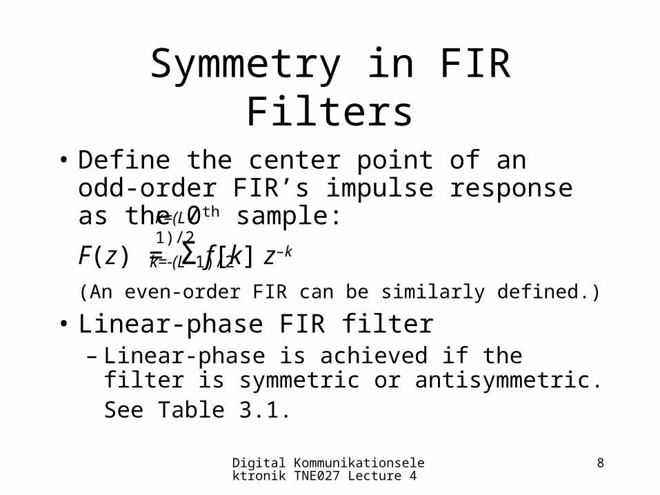
Symmetry in FIR Filters

• Define the center point of an odd-order FIR’s impulse response as the 0th sample:

F(z) = Σ f[k] z–k

(An even-order FIR can be similarly defined.)

• Linear-phase FIR filter– Linear-phase is achieved if the filter is

symmetric or antisymmetric.See Table 3.1.

k=(L-1)/2

k=-(L-1)/2


9

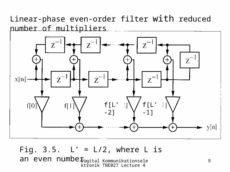
Fig. 3.5. L’ = L/2, where L is an even number.

Linear-phase even-order filter with reduced number of multipliers

f[L’-1]f[L’-2]


10

Constant Coefficient FIR Design

• There are only a few applications, e.g., adaptive filters, where we need a general programmable filter.

• In many applications, the filters are Linear Time Invariant (LTI) and the coefficients do not change over time.

• The hardware effort can be reduced for constant coefficient FIR.


11

Direct FIR implementation

• In a practical situation, the FIR coefficients are obtained from a computer design tool and presented to the designer as floating point numbers.

• The performance of a fixed-point FIR, based on the floating-point coefficients, should be verified using simulation or algebraic analysis to ensure that design specifications remain satisfied.


12

• Dynamic range overflow should be avoided.

• The worst-case dynamic range growth G of an Lth- order FIR is

G log2(Σ |f[k]|)

See Example 3.2: Four-tap direct FIR filter.

L-1

k=0


13

Improve the direct FIR design

1. Realize each filter coefficient with an optimal CSD code.

2. Increase effective multiplier speed by pipelining.

3. For FIR with symmetric coefficients, the number of multipliers can be reduced.

See Table 3.3 and Example 3.3.


14

Rephasing pipelined multiplier in FIR filter

Add a positive delay

f[n]=z d f[n] z -d


15

FIR Filter with Transposed Structure

• If the transposed filter has constant coefficients, two improved designs should be considered:– Multiple use of the repeated coefficients using

the reduced adder graph (RAG) algorithm– Pipeline adders


16

Reduced Adder Graph

Algorithm 3.4: Reduced Adder Grapha) Remove the sign of the coefficient.

b) Remove all coefficients and factors that are a power of two.

c) Realize all cost “1” coefficients.

d) Use cost “1” coefficients in building the multiplier of higher cost. (Use Table 2.3.)

See Example 3.5.


17

Reduced Adder Graph for F6 Half-band Filter

Fig. 3.11. Realization of F6 using RAG algorithm


18

FIR Filter Using Distributed Arithmetic

• Distributed Arithmetic Using Logic Cells See Example 3.6: Distributed Arithmetic Filter as State Machine.– Logic cells are used to implement small look-

up tables for low-order filters.– The outputs of a collection of low-order filters

can be added together to define the output of a high-order FIR.

See Example 3.7: Five-input DA Table.


19

• DA Using Embedded Array Blocks– It is not economical to use the 2-kbit EABs for

a short FIR filter, mainly because the number of available EABs is limited.

– The maximum registered speed of an EAB is 76 MHz, and an LC table implementation may be faster for a short FIR filter.

– For long filters, EABs have registered throughput at a constant 76 MHz and routing effort is reduced.See Example 3.8: Distributed Arithmetic Filter using EABs.


20

Fig. 3.16: Parallel implementation of a distributed arithmetic FIR filter

Example 3.10: Loop Unrolling for DA FIR Filter

digital kommunikationselektronik tne027 lecture 4 1 finite impulse response (fir) digital filters...

Documents