digital modulation 04 - massey university modulation_04_1s.pdf · – provide an overview of...

Digital Modulation – Lecture 04

FiltersDigital Modulation Techniques

© Richard Harris

Communication Systems 143.332 - Digital Modulation Slide 2

Objectives

• To be able to discuss the purpose of filtering and determine the properties of well known filters.

• You will be able to:– Describe I/Q diagrams and their uses– Provide an overview of digital modulation application areas– Describe the characteristics of the various forms of filters and

their use in digital transmission


Presentation Outline

• Filtering methods– Raised cosine– Square-root raised cosine– Gaussian filters

• Detection methods for standard Digital Modulation techniques

• PSDs for common Digital Modulation schemes


References

• Digital Modulation in Communication Systems – An Introduction (Hewlett Packard Application Note 1298)

• Principles of Digital Modulation, by Dr Mike Fitton, [email protected] Telecommunications Research Lab Toshiba Research Europe Limited


Filtering – 1

• Filtering allows the transmitted bandwidth to be significantly reduced without losing the content of the digital data.

• Spectral efficiency of the signal is improved using filtering.• Many possible varieties:

– Raised cosine– Square-root raised cosine– Gaussian filters

• Any fast transition in a signal, irrespective of whether it is amplitude, phase or frequency, will need wide occupied bandwidth.

• Thus, if we have a technique that can help to slow down these transitions then it will narrow the occupied bandwidth.


Filtering – 2

• Filtering helps to smooth these transitions (in I and Q).• It also reduces interference since it lowers the

tendency of one signal to interfere with another.• On the receiver side, the reduced bandwidth increases

the sensitivity because more noise and interference are rejected.

• Tradeoffs may be necessary though:– Some types of filtering may cause the trajectory of the signal

(the paths of transitions between states) to overshoot .– Overshooting implies more carrier power and phase from the

transmitter amplifiers


Filtering – 3

• Other problems– Filtering may make radios more complex and larger.– Filtering can create ISI problems

• Can occur if heavy filtering so that the symbols blur together and each symbol affects those around it .

• This is determined by the time response or the impulse response of the filter.


Nyquist or Raised-Cosine Filters

• The following graph shows the impulse or time domain response of a Nyquist filter. – We have seen this figure before.

• Nyquist filters have the property that their impulse response rings at the symbol rate.

• The filter is chosen to ring or have the impulse response of the filter cross through zero at the symbol clock frequency.

0

1f



• The time response of the filter goes through zero with a period that exactly corresponds to the symbol spacing.

• Adjacent symbols do not interfere with each other at the symbol times because the response equals zero at all symbol times except the centre (desired) one.

• Nyquist filters heavily filter the signal without blurring the symbols together at the symbol times.

• This is important for transmitting information without errors caused by Inter-Symbol Interference.

• Note that Inter-Symbol Interference does exist at all times except the symbol (decision) times.

• Usually the filter is split, half being in the transmit path and half in the receiver path.

• In this case root Nyquist filters (commonly called root raised cosine) are used in each part, so that their combined response is that of a Nyquist filter.



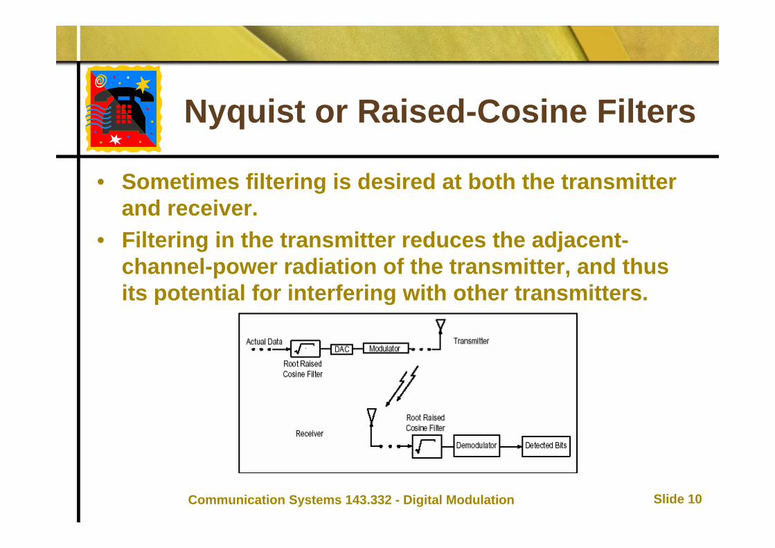
• Sometimes filtering is desired at both the transmitter and receiver.

• Filtering in the transmitter reduces the adjacent-channel-power radiation of the transmitter, and thus its potential for interfering with other transmitters.



• Filtering at the receiver reduces the effects of broadband noiseand also interference from other transmitters in nearby channels.

• To get zero Inter-Symbol Interference (ISI), both filters are designed until the combined result of the filters and the rest of the system is a full Nyquist filter.

• Potential differences can cause problems in manufacturing because the transmitter and receiver are often manufactured by different companies.– The receiver may be a small hand-held model and the transmitter

may be a large cellular base station. – If the design is done correctly, the results are the best data rate, the

most efficient radio, and reduced effects of interference and noise. • This is why root-Nyquist filters are used in receivers and

transmitters as √Nyquist x √Nyquist = Nyquist. • Matched filters are not used in Gaussian filtering.


Gaussian Filter - 1

• In contrast, a GSM signal will have a small blurring of symbols on each of the four states because the Gaussian filter used in GSM does not have zero Inter-Symbol Interference.

• The phase states vary somewhat causing a blurring of the symbols as shown in the figure below.

• Wireless system architects must decide just how much of the Inter-Symbol Interference can be tolerated in a system and combine that with noise and interference.


Gaussian Filter – 2


Gaussian Filter – 3

• Gaussian filters are used in GSM because of their advantages in carrier power, occupied bandwidth and symbol-clock recovery.

• The Gaussian filter is a Gaussian shape in both the time and frequency domains, and it does not ring like the raised cosine filters do.

• Its effects in the time domain are relatively short and each symbol interacts significantly (or causes ISI) with only the preceding and succeeding symbols.

• This reduces the tendency for particular sequences of symbols to interact which makes amplifiers easier to build and more efficient.


Filter Bandwidth Parameter r - 1

• The sharpness of a raised cosine filter is described by the value of r – the roll-off parameter.

• Thus r gives a direct measure of the occupied bandwidth of the system and is calculated as

Occupied bandwidth = Symbol rate X (1 + r).• If the filter had a perfect characteristic with sharp

transitions and r = 0, the occupied bandwidth would be:

Occupied bandwidth = Symbol rate X (1 + 0) = symbol rate.



• An r-value of one uses twice as much bandwidth as an r-value of zero.

• In practice, it is possible to implement an r-value below 0.2 and make good, compact, practical radios. – Typical values range from 0.35 to 0.5, though some video

systems use an r-value as low as 0.11. The corresponding term for a Gaussian filter is BT (bandwidth time product).

• Occupied bandwidth cannot be stated in terms of BT because a Gaussian filter’s frequency response does not go identically to zero, as does a raised cosine.

• Common values for BT are 0.3 to 0.5.


Different Filter Bandwidths

• Different filter bandwidths show different effects. For example, look at a QPSK signal and examine how different values of r effect the vector diagram. If the radio has no transmitter filter as shown on the left of the graph, the transitions between states are instantaneous. No filtering means an r of infinity.

Power Spectral Densities and Detection Methods for Digital Modulation

© Richard Harris


Coherent Reception

• An estimate of the channel phase and attenuation is recovered. It is then possible to reproduce the transmitted signal, and demodulate. It is necessary to have an accurate version of the carrier, otherwise errors are introduced.

• Carrier recovery methods include:– Pilot Tone (such as Transparent Tone in Band)– Less power in information bearing signal– High peak-to-mean power ratio

• Pilot Symbol Assisted Modulation– Less power in information bearing signal

• Carrier Recovery (such as Costas loop)– The carrier is recovered from the information signal


Differential Reception

• In the transmitter, each symbol is modulated relative to the previous symbol, for example in differential BPSK:– 0 = no change 1 = +180o

• In the receiver, the current symbol is demodulated using the previous symbol as a reference. – The previous symbol acts as an estimate of the channel.

• Differential reception is theoretically 3dB poorer than coherent. This is because the differential system has two sources of error: – a corrupted symbol, and – a corrupted reference (the previous symbol).

• Non-coherent reception is often easier to implement.


Computing the PSD of OOK

• The Power Spectral Density of the complex envelope is computed using our PSD formula as:

• Assuming that m(t) has a peak value of • The PSD of OOK is then given by

22 sin( ) ( )2c b

g bb

A fTP f f TfTπδ

π

⎡ ⎤⎛ ⎞⎢ ⎥= + ⎜ ⎟⎢ ⎥⎝ ⎠⎣ ⎦

2

1 ( ) ( )4 g c g cP f f P f f⎡ ⎤− + − −⎣ ⎦

Note: We have already considered this in a tutorial


Plot of PSD for OOK

• The null-null bandwidth is 2R• The transmission bandwidth

of OOK is BT = 2B where B is the baseband bandwidth

• With raised cosine rollofffiltering, B= ½(1+r)R, hence– BT = (1+r)R

• Note:– For binary signalling, D = R.


Detection of OOK – 1

• The following set up is used to detect OOK signals:

OOK in Envelopedetector

Binary output

Non-coherent Detection

Coherent Detection with Low-Pass Filter Processing

Low-passfilter

Binary outputOOK in


Detection of OOK – 2

• Note:– When the received OOK signal is corrupted by Additive White

Gaussian Noise (AWGN), the optimal detection (to obtain the lowest possible Bit Error Rate – BER ) requires coherent detection with matched filter processing.


Binary Phase-Shift Keying

• Computing the PSD for the complex envelope of BPSK gives the following:

• Assuming that m(t) has peak values of ±1• The PSD of BPSK is then given by

22 sin)( ⎟⎟

⎠

⎞⎜⎜⎝

⎛=

b

bbcg fT

fTTAfPππ

[ ])()(41

cgcg ffPffP −−+−


The PSD of BPSK

• The bandwidth for BPSK is the same as for OOK.• Raised cosine-rolloff filtering can be used to conserve

bandwidth


Detection of BPSK

• recovers m(t)• Coherent detection must be used.[ ]( )( sin c LPs t tω−


Orthogonal Signalling – 1

• Consider transmitting a binary 1 over the bit interval 0<t<Tb using an FSK signal given by:

• The binary 0 is transmitted using the signal

• Where θ1 = θ2 for continuous phase FSK, the two signals are orthogonal if

• That is:2

1 1 2 20cos( )cos( ) 0bT

cA t t dtω θ ω θ+ + =∫

1 20( ) ( ) 0bT

s t s t dt =∫

1 1 1( ) cos( )cs t A tω θ= +

2 2 2( ) cos( )cs t A tω θ= +



• This means that

• The second term is negligible since we assume ω1+ω2is large.

• Therefore

21 2 1 2 1 2

1 2

21 2 1 2 1 2

1 2

sin[( ) ( )] sin( )2 ( )

sin[( ) ( )] sin( ) 02 ( )

c b

c b

A T

A T

ω ω θ θ θ θω ω

ω ω θ θ θ θω ω

⎡ ⎤− + − − −⎢ ⎥−⎣ ⎦⎡ ⎤+ + + − +

+ =⎢ ⎥+⎣ ⎦

1 2 1 2sin[2 ( )] sin( ) 02

hh

π θ θ θ θπ

+ − − −=



• Where

• For θ1 = θ2 the minimum value for orthogonality is h=0.5, or a peak frequency deviation of

• For θ1 ≠ θ2 the discontinuous phase FSK case, the minimum value for the orthogonality is h=1, or a peak frequency deviation of

1 2( ) 2 (2 )and

2

b b

b

T F T

h FT

ω ω π− = ∆

= ∆

1 14 4b

F RT

∆ = =

1 12 2b

F RT

∆ = =


Minimum Shift Keying (MSK)

• Minimum Shift Keying is continuous phase FSK with a minimum modulation index (h=0.5) that will produce orthogonal signalling.

• The complex envelope is

• Where ∆F= ¼R and m(t) = ±1• MSK is a constant amplitude signal

( )( )( )t

m dj tc cg t A e A e

λ λθ −∞∫= =


MSK – 2

• MSK can be generated by using a simple FM modulator, viz:

• MSK is equivalent to OQPSK with sinusoidal pulse shaping.

FM Transmitter∆F= ¼R


PSD of MSK

• The PSD of the complex envelope is given by:

2 2

2 2 2

16 cos 2( )[1 (4 ) ]

c b bg

b

A T T fP fT fπ

π⎛ ⎞

= ⎜ ⎟−⎝ ⎠


GMSK – 1

• Gaussian-filtered MSK– The data (rectangular shaped pulses) are filtered by a filter

having a Gaussian shaped frequency response

– Where B is the 3dB bandwidth of the filter• The PSD of GMSK can be obtained via computer

simulation

2( / ) (ln 2 / 2)( ) f BH f e⎡ ⎤−⎣ ⎦=


GMSK – 2

• BTb = 0.3 (ie. the 3dB bandwidth is 0.3 of the bit rate) gives a good compromise for relatively low side-lobes and tolerable ISI

• GMSK has a constant envelope• GMSK with BTb = 0.3 is the modulation format used in

GSM cellular telephone systems• GMSK and MSK can be detected either coherently or

non-coherently


Detection of DPSK

• Partially coherent detection:– Does not require carrier phase synchronisation

• Receiver detects the relative phase difference between the waveforms of en and en-1 to determine dn

• In the previous example, dn=1 if phase difference is πand dn=0 if no phase difference


PSD of FSK

• h is the digital modulation index, the peak frequency deviation for m(t) having values of ±1.

• (See pages 349-351 for the mathematical expression for the PSD in this case)

/ 2fF D π∆ =


Bandwidth of FSK

• The approximate bandwidth is given by Carson’s rule:

• Where and B is the bandwidth of the square-wave data waveform.

• Using the first null bandwidth, B=R, thus

• With raised cosine filtering, B = 1/2 (1+r)R, hence

2( 1)TB Bβ= +

/F Bβ = ∆

2( )TB F R= ∆ +

2 (1 )TB F r R= ∆ + +


Detection of FSK

digital modulation 04 - massey university modulation_04_1s.pdf · – provide an overview of...

Documents