digital programmable gaussian noise generator · digital programmable gaussian noise generator wpi...
TRANSCRIPT

1
Digital Programmable Gaussian Noise Generator
WPI – MIT Lincoln Laboratory
A Major Qualifying Project
Submitted to the faculty of the WORCESTER POLYTECHNIC INSTITUTE in partial fulfillment of the requirements for the
Degree of Bachelor of Science in Electrical and Computer Engineering
by
________________________________
Karen L. Fitch Date: October 30, 2015
________________________________
Kathryn A. Gillis Date: October 30, 2015
________________________________
Abby W. Harrison Date: October 30, 2015
Approved: ________________________________
Edward A. Clancy, Faculty Advisor, WPI
Date: October 30, 2015
This work is sponsored by the Department of the Air Force under Air Force Contract #FA8721-05-C-0002. Opinions, interpretations, conclusions, and recommendations are those of the
authors and not necessarily endorsed by the United States Government.
2
Abstract Electronic countermeasures are critical to air vehicle survivability. Noise jamming is a
technique used to prevent radar from tracking targets by taking advantage of a radar’s sensitivity
to noise. Gaussian noise is preferred for this purpose because it is more difficult to eliminate than
structured noise. This project produced a digital Gaussian noise generator based around a field
programmable gate array (FPGA) with programmable bandwidth, center frequency, and
amplitude to be used by Group 108 within MIT Lincoln Laboratory. Noise produced by the
generator is band limited white in frequency with a Gaussian probability density function, as
verified both visually and via statistical tests. The device is a strong improvement over existing
technology used by Group 108 and it will be used in laboratory and over-the-air testing for
researching the effects of Gaussian noise on various radar systems.

3
Statement of Authorship
In this project, all three group members contributed to work on all parts of the design and
implementation of the final device. All members also contributed to editing all sections of the
paper, but sections were written individually as follows:
Karen Fitch: Sections 1.0, 2.5, 3.1, 3.2, Chapter 6 Kathryn Gillis: Sections 2.1, 2.3, 3.4.1, 3.4.3, Chapter 4 Abby Harrison: Sections 2.2, 2.4, 3.3, 3.4.2, 3.4.3, Chapter 5 All members wrote the Abstract and Executive Summary

4
Acknowledgements
We would like to thank Lisa Basile, Sarah Curry, Emily Fenn and Chris Massa for
mentoring us throughout our time at MIT Lincoln Laboratory and for assisting us in
understanding and completing our project. We would also like to thank Professor Edward
Clancy, our WPI advisor, for guiding us and consistently encouraging us to improve our project.
Additional thanks go to Dave Baur, Jim Burke, Bob Giovanucci, Dave McQueen and Andy
Messier for their important contributions to our project.
5
Table of Contents
Abstract ........................................................................................................................................... 1
Statement of Authorship ................................................................................................................. 3
Acknowledgements ......................................................................................................................... 4
Table of Contents ............................................................................................................................ 5
Table of Figures .............................................................................................................................. 7
Table of Tables ............................................................................................................................... 9
Executive Summary ...................................................................................................................... 10
2.0 Background ............................................................................................................................. 15 2.1 Gaussian Noise and Radar ................................................................................................... 15
2.1.1 Radar Overview ............................................................................................................ 15 2.1.2 Radar Pulse Generation ................................................................................................ 16 2.1.3 Effects of Noise on Radar ............................................................................................. 19 2.1.4 Jamming Techniques .................................................................................................... 19 2.1.5 Effectiveness of White Gaussian Noise in Jamming .................................................... 20
2.2 Gaussian Characteristics ..................................................................................................... 20 2.2.1 Defining Characteristics ............................................................................................... 20 2.2.2 How to Test Characteristics .......................................................................................... 24
2.3 Group 108 Testing Environment ......................................................................................... 27 2.3.1 Radar Open Systems Architecture ................................................................................ 27 2.3.2 Existing Noise Sources in Group 108 ........................................................................... 28
2.4 Digital Generation of Gaussian Noise ................................................................................. 28 2.4.2 Pseudorandom Number Generation .............................................................................. 29 2.4.3 Techniques for Digitally Generating Gaussian Distributions ....................................... 29
2.5 Digital Programmability ...................................................................................................... 33 2.5.1 Center Frequency and Bandwidth ................................................................................ 33 2.5.2 Amplitude ..................................................................................................................... 37
3.0 Methods................................................................................................................................... 38 3.1 Project Requirements .......................................................................................................... 38 3.2 Gaussian Test Suite ............................................................................................................. 39 3.3 Hardware Selection ............................................................................................................. 39 3.4 Implementation .................................................................................................................... 40
3.4.1 Random Number Algorithm Selection and Implementation ........................................ 40 3.4.2 Programmability ........................................................................................................... 48 Determining Center Frequency and Bandwidth .................................................................... 48 User Interface ........................................................................................................................ 51
6
4.0 Results ..................................................................................................................................... 54 4.1 Simulation Results .............................................................................................................. 54 4.2 Output Test Results ............................................................................................................. 60 4.3 ROSA Data .......................................................................................................................... 64
5.0 Discussion ............................................................................................................................... 66
6.0 Conclusion .............................................................................................................................. 70
Works Cited .................................................................................................................................. 72
Appendix A – Hardware Platform Value Analysis ....................................................................... 75
Appendix B – MATLAB Simulation of Uniform Data Through ROSA ...................................... 76
7
Table of Figures Figure 1: Comparison of KC705 Noise Generator to WhiteBox Lite Noise ................................ 13
Figure 2: IQ Data .......................................................................................................................... 16
Figure 3: Mixing a signal to a desired center frequency ............................................................... 17
Figure 4: IQ data generation by digital mixing (top) and analog mixing (bottom) ...................... 18
Figure 5: MATLAB-generated autocorrelation of white Gaussian noise vs. band-limited Gaussian noise ....................................................................................................................... 21
Figure 6: MATLAB-generated power spectral density plots of white vs. band-limited noise ..... 22
Figure 7: Gaussian distribution with zero-mean and standard deviation of 1 .............................. 23
Figure 8: Rayleigh distribution with σ = 1 .................................................................................... 24
Figure 9: Visualizing chi-square null hypothesis testing .............................................................. 26
Figure 10: Overview of data acquisition using ROSA ................................................................. 27
Figure 11: Gaussian ICDF ............................................................................................................ 30
Figure 12: Ziggurat Resolution Comparison ................................................................................ 32
Figure 13: Ideal vs Practical Band Pass Filter .............................................................................. 34
Figure 14 Filter Flow Diagrams .................................................................................................... 35
Figure 15: Cascaded 2nd Order IIR Filter .................................................................................... 36
Figure 16: Broadband vs. Baseband Generation ........................................................................... 37
Figure 17: High Level Integration Diagram ................................................................................. 39
Figure 18: Diagram of Fixed-Point Box-Muller Algorithm Implementation ............................... 45
Figure 19: Block Diagram of Second Box-Muller Implementation ............................................. 46
Figure 20: Calculating an FIR Band pass Filter Response ........................................................... 51
Figure 21: FPGA-based digital noise generator ............................................................................ 54
Figure 22: Power Spectrum of MATLAB Simulated Data .......................................................... 55
Figure 23: Time Domain Distribution of MATLAB Simulated Data .......................................... 56
Figure 24: Power Spectrum of Fixed-Point Box-Muller Hardware Simulation ........................... 57
Figure 25: Time Domain Distribution of Fixed-Point Box-Muller Hardware Simulation ........... 58
Figure 26: Power Spectrum of Floating-Point Box-Muller Hardware Simulation ....................... 59
8
Figure 27: Time Domain Distribution of Floating-Point Box-Muller Hardware Simulation ....... 59
Figure 28: KC705 Broadband Noise Power Spectrum ................................................................. 60
Figure 29: KC705 Time Domain Distribution of Broadband Noise ............................................. 61
Figure 30: Power Spectrum of Band-limited Noise with Bandwidth and Center Frequency of 30 MHz (3 dB cutoffs marked) ................................................................................................... 62
Figure 31: Time Domain Distribution of Band-limited Noise ...................................................... 62
Figure 32: Power Spectrum of WhiteBox Lite Frequency Sweep ................................................ 63
Figure 33: Time Domain Distribution of WhiteBox Lite Frequency Sweep ................................ 63
Figure 34: Time Domain Distribution ROSA Data from Fixed-Point Box-Muller ...................... 65
Figure 35: Time Domain Distribution ROSA Data from WhiteBox Lite .................................... 65

9
Table of Tables Table 1: Result Comparison .......................................................................................................... 12
Table 2: MATLAB randn p-values ............................................................................................... 56
Table 3: Fixed-Point Simulation p-values .................................................................................... 58
Table 4: Floating-Point Simulation p-values ................................................................................ 59
Table 5: Floating-Point Broadband Oscilloscope Data p-values .................................................. 61
Table 6: Floating-Point Band-Limited Oscilloscope Data p-values ............................................. 62
Table 7: WhiteBox Lite p-values .................................................................................................. 64
Table 8: Table of FPGA Resources Utilized ................................................................................ 68
10
Executive Summary The objective of our project was to design and implement a digital, programmable,
intermediate frequency (IF) band Gaussian noise generator for Group 108 at MIT Lincoln
Laboratory. The Group conducts research on tactical defense and intelligence, surveillance, and
reconnaissance (ISR) systems and is interested in the effects of Gaussian versus structured noise
on radar.
Pulsed radar is a surveillance technique widely used for aerial defense. This surveillance
technique detects targets by emitting a high frequency signal and identifying returned signals that
have reflected off of an object. The radar locates targets by comparing the power of a received
signal in a given direction to a threshold determined by the system. The amount of noise in a
radar system influences its performance. Noise in the radar system comes from both electrical
components in the receiver and the environment. Jamming is an electronic counter-measure
technique that takes advantage of threshold detection sensitivity to noise to deny or deceive radar
detection of targets. One jamming method is emission of a structured signal that matches a
radar’s pulse, which causes the radar to detect a false target. Another jamming method is
emission of unstructured noise in order to mask reflected signals within the increased noise
received by the radar. Group 108 currently has strong capabilities for generating false targets, but
is looking to expand their noise jamming abilities. Generation of Gaussian noise is an area of
interest for noise jamming since the noise inherent in radar systems is also Gaussian. [Eaves,
1987; Nitzberg, 1999]
The noise generated by electrical components in radar receivers is approximated as white
Gaussian noise. White noise is defined as noise that has equal power at all frequencies. Gaussian
noise is a random signal that has a normal, bell-shaped probability density function (PDF).
Generating wideband white Gaussian noise is not achievable in practice since infinite-valued
noise amplitudes and frequencies are purely theoretical. In actuality, white Gaussian noise is
always band-limited due to physical constraints and is only white within its frequency band.
We designed a digital noise generator on standalone hardware that produces band-
limited, white Gaussian noise with programmable amplitude, center frequency, and bandwidth.
We implemented the generator on the Xilinx Kintex-7 DSP Development Kit (KC705), a
development board with a large Kintex-7 FPGA and a daughtercard containing a dual channel,
16-bit digital-to-analog converter (DAC). Data for the implementation were collected using

11
Xilinx ISim testbench simulations, a spectrum analyzer, and an oscilloscope. We did not collect
data for our noise generator on Group 108’s test and development system as the processing
performed by the system distorted the acquired data. To test the whiteness and normality of our
results, we created a MATLAB test suite that qualitatively evaluates a data set based on its
autocorrelation, power spectral density (PSD), and histogram. Additionally, quantitative
measurements are provided using the chi-square test and the Anderson-Darling test. To reduce
the effects of random variations in the data, we averaged results from five runs over a standard
sample size of 100,000 per run.
Group 108 currently uses the KC705 with their radar test and development system to
produce false targets for jamming using a system called WhiteBox Lite. We used the source code
for this device as a base for our design. Our KC705 implementation generates either broadband
or band-limited white Gaussian noise with a maximum bandwidth of 0 to 125 MHz by
transforming uniformly distributed, pseudorandom numbers to normally distributed numbers.
The numbers are optionally processed through a filter and amplitude control and then converted
to an analog signal using a DAC. The uniform numbers are generated using a Tausworthe
algorithm based on linear feedback shift registers and transformed using the Box-Muller
algorithm. The original implementation used fixed-point calculations, while a later improvement
changed the algorithm to use floating point calculations to improve the statistical quality of the
Gaussian output. The floating point implementation makes use of Xilinx modules, which are
fully pipelined to produce one output every clock cycle. The device is programmable through a
command line interface which uses a terminal window to send serial commands to a soft
processor on the FPGA. The amplitude is controlled by multiplying the output values by an
attenuation factor while a finite impulse response band pass filter controls the center frequency
and bandwidth.
Before testing the KC705, we collected data from MATLAB-simulated Gaussian noise,
an analog Gaussian noise generator, and a digital noise source used by Group 108. These data
were collected using the Group’s radar test and development system, except for the MATLAB
simulation. Based on analysis of the preliminary data, we set a benchmark where our noise
generator must pass the chi-square and Anderson-Darling tests. These tests produce a test
statistic called a p-value that we require to be at least 0.2. For goodness-of-fit tests to a Gaussian
distribution, a higher p-value indicates a closer fit. A commonly used significance level is 0.05
12
when researchers are trying to show that their data are statistically significant rather than
random. We opted to raise the threshold to meet the lowest value scored by MATLAB’s randn
function, which also produces pseudorandom, normally distributed numbers.
We performed analysis on both the in-phase (I) and quadrature (Q) components of our
output, both of which were Gaussian, as well as the signal with combined components, which
had a Rayleigh distribution. The simulation data passed all of our tests with comparable quality
to an analog noise generator. The chi-square and Anderson-Darling test results were a significant
improvement over the existing WhiteBox Lite noise and are comparable to both the MATLAB
simulation and a commercially available analog noise source. The physical data collected using
the spectrum analyzer showed that output is white up to approximately 80 MHz, with attenuation
at higher frequencies. The physical data collected using the oscilloscope showed that the analog
noise is visually Gaussian, though with less statistical quality than its simulated counterpart. A
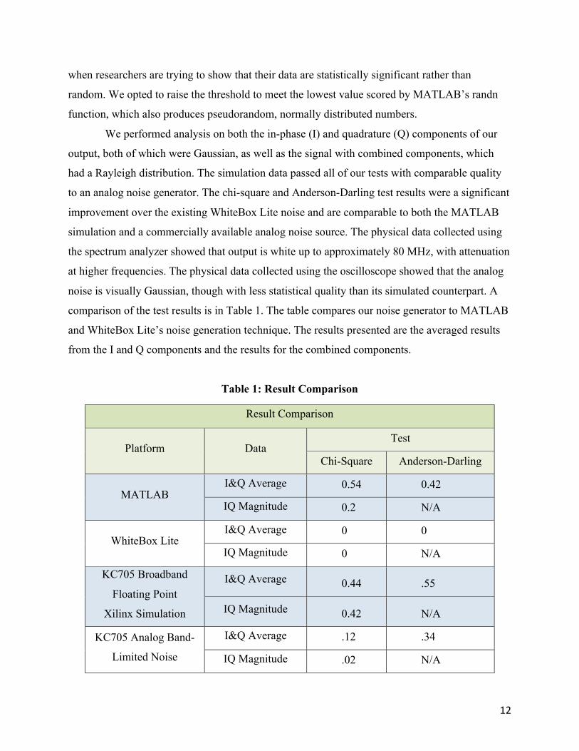
comparison of the test results is in Table 1. The table compares our noise generator to MATLAB
and WhiteBox Lite’s noise generation technique. The results presented are the averaged results
from the I and Q components and the results for the combined components.
Table 1: Result Comparison
Result Comparison
Platform Data Test
Chi-Square Anderson-Darling
MATLAB I&Q Average 0.54 0.42
IQ Magnitude 0.2 N/A
WhiteBox Lite I&Q Average 0 0
IQ Magnitude 0 N/A
KC705 Broadband
Floating Point
Xilinx Simulation
I&Q Average 0.44 .55
IQ Magnitude 0.42 N/A
KC705 Analog Band-
Limited Noise
I&Q Average .12 .34
IQ Magnitude .02 N/A
13
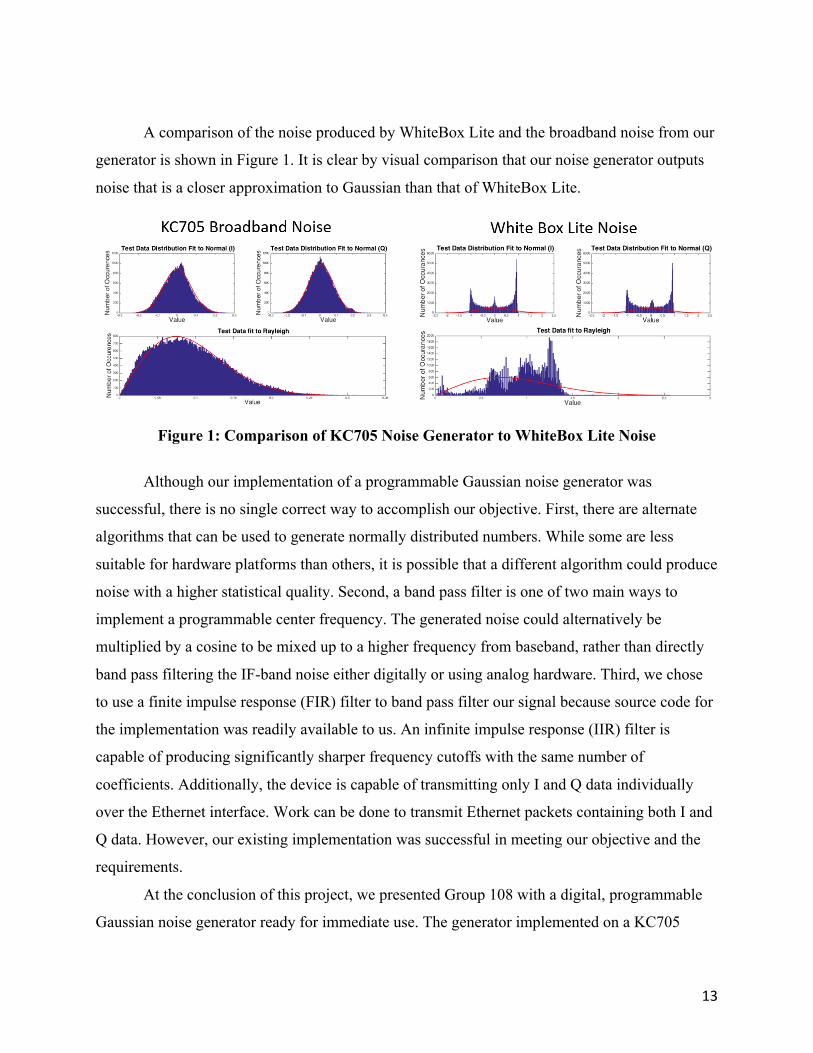
A comparison of the noise produced by WhiteBox Lite and the broadband noise from our
generator is shown in Figure 1. It is clear by visual comparison that our noise generator outputs
noise that is a closer approximation to Gaussian than that of WhiteBox Lite.
Figure 1: Comparison of KC705 Noise Generator to WhiteBox Lite Noise
Although our implementation of a programmable Gaussian noise generator was
successful, there is no single correct way to accomplish our objective. First, there are alternate
algorithms that can be used to generate normally distributed numbers. While some are less
suitable for hardware platforms than others, it is possible that a different algorithm could produce
noise with a higher statistical quality. Second, a band pass filter is one of two main ways to
implement a programmable center frequency. The generated noise could alternatively be
multiplied by a cosine to be mixed up to a higher frequency from baseband, rather than directly
band pass filtering the IF-band noise either digitally or using analog hardware. Third, we chose
to use a finite impulse response (FIR) filter to band pass filter our signal because source code for
the implementation was readily available to us. An infinite impulse response (IIR) filter is
capable of producing significantly sharper frequency cutoffs with the same number of
coefficients. Additionally, the device is capable of transmitting only I and Q data individually
over the Ethernet interface. Work can be done to transmit Ethernet packets containing both I and
Q data. However, our existing implementation was successful in meeting our objective and the
requirements.
At the conclusion of this project, we presented Group 108 with a digital, programmable
Gaussian noise generator ready for immediate use. The generator implemented on a KC705

14
development board met the needs of the Group. Our final design is a small, standalone platform
that produces band-limited, white Gaussian noise with programmable amplitude, center
frequency, and bandwidth. This platform will enhance Group 108’s radar research and test
capabilities.
15
2.0 Background
This chapter will provide background information necessary for the development of our
digital, programmable, Gaussian noise generator. Section 2.1 first gives general information on
what radar is, how it works, and why Gaussian noise is effective for jamming applications.
Second, section 2.2 covers the characteristics of Gaussian noise and testing how close a sample
distribution is to an ideal Gaussian distribution. Third, section 2.3 describes the need and purpose
for a digital, programmable, Gaussian noise generator in Group 108’s radar testing and
development system. Finally, sections 2.4 and 2.5 explain how to digitally generate Gaussian
noise and techniques that can be used to configure the noise.
2.1 Gaussian Noise and Radar Before discussing digitally generated Gaussian noise, it is important to provide basic
background on how radar works and why Gaussian noise is important to radar research.
2.1.1 Radar Overview Radar is a common tool used in many contexts, such as air traffic control and aerial
defense, to find and track targets that cannot be easily tracked visually. Pulsed radar systems
detect objects by sending a sinusoidal pulse of electromagnetic radiation into the environment at
a high frequency and checking for any reflection of the pulse that returns to the radar. If the
return voltage from a pulse is above a certain threshold, the system assumes that the radiated
waveform reflected off an object within the antenna’s beam, resulting in target detection. The
radiation’s constant velocity and the time to return can then be used to calculate the distance to
the object, R, that caused the reflection by using the relation in Equation 1 where c is the speed
of light. Additionally, the Doppler shift in the frequency of the returned signal gives the target’s
approximate radial velocity. [Eaves, 1987; Nitzberg, 1999]
𝑡" = 𝑑𝑖𝑠𝑡𝑎𝑛𝑐𝑒𝑣𝑒𝑙𝑜𝑐𝑖𝑡𝑦 =
2𝑅𝑐 Eq. 1.
16
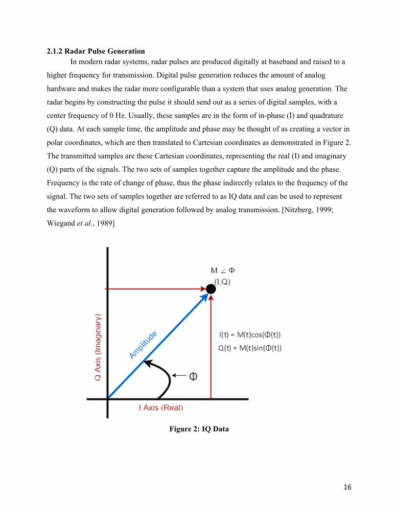
2.1.2 Radar Pulse Generation In modern radar systems, radar pulses are produced digitally at baseband and raised to a
higher frequency for transmission. Digital pulse generation reduces the amount of analog
hardware and makes the radar more configurable than a system that uses analog generation. The
radar begins by constructing the pulse it should send out as a series of digital samples, with a
center frequency of 0 Hz. Usually, these samples are in the form of in-phase (I) and quadrature
(Q) data. At each sample time, the amplitude and phase may be thought of as creating a vector in
polar coordinates, which are then translated to Cartesian coordinates as demonstrated in Figure 2.
The transmitted samples are these Cartesian coordinates, representing the real (I) and imaginary
(Q) parts of the signals. The two sets of samples together capture the amplitude and the phase.
Frequency is the rate of change of phase, thus the phase indirectly relates to the frequency of the
signal. The two sets of samples together are referred to as IQ data and can be used to represent
the waveform to allow digital generation followed by analog transmission. [Nitzberg, 1999;
Wiegand et al., 1989]
Figure 2: IQ Data

17
This signal is then mixed with sinusoidal waves at an intermediate frequency (IF)
between 0 Hz and the frequency at which it will be transmitted. The I data are multiplied by a
wave of the form cos(2πfct) and the Q data by a wave of the form sin(2πfct). As the signal must
be transmitted as an analog pulse, the I and Q data are combined and converted to an analog
waveform using a digital to analog converter (DAC). The amplitude of the analog pulse is the
square root of the sum of the squares of the I and Q data, while the phase is the inverse tangent of
Q divided by I. Finally, the pulse is multiplied by another sine wave, this time in the analog
domain, to shift its frequency up to the transmission radio frequency (RF) the radar uses. The
process of multiplying the signal with sine waves is known as mixing. At each stage, the signal is
shifted up by the frequency of the sine wave, as seen in Figure 3. Replicas are also created at
integer multiples of the sine wave frequency, which must be removed through filtering. Analog
mixing is often useful for bypassing the limitations of the DAC. Without mixing, the maximum
transmit frequency is limited to half the DAC output rate; with mixing, the maximum frequency
is limited by the analog mixing hardware.
Signalf f
Sine Wave fc
f-fc fcSignal Mixed to fc
-fc
Figure 3: Mixing a signal to a desired center frequency
When the return signal is received, the same process is performed in reverse. IQ data
points are created by mixing the received signal with cosine and sine waves at the signal’s center
frequency to produce two separate signals centered at 0 Hz or at IF. These signals are then low
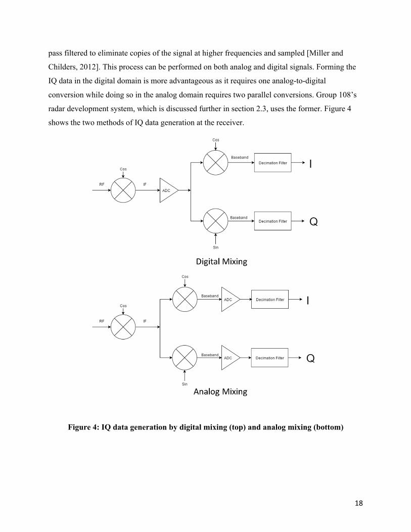
18
pass filtered to eliminate copies of the signal at higher frequencies and sampled [Miller and
Childers, 2012]. This process can be performed on both analog and digital signals. Forming the
IQ data in the digital domain is more advantageous as it requires one analog-to-digital
conversion while doing so in the analog domain requires two parallel conversions. Group 108’s
radar development system, which is discussed further in section 2.3, uses the former. Figure 4
shows the two methods of IQ data generation at the receiver.
Figure 4: IQ data generation by digital mixing (top) and analog mixing (bottom)

19
2.1.3 Effects of Noise on Radar There are many factors in radar detection that add to the complexity of the simplified
explanation above. One of the most prominent is detection in noise. Detection is the process by
which a target is sensed in the presence of competing returns that come from background echoes,
atmospheric noise, or noise generated in the radar receiver. Noise forces the radar to perform a
careful balancing act as its effects can increase or decrease the detected return voltage depending
on whether the interference is constructive or destructive. If the radar has too low a threshold for
detecting a target, noise that adds to the return voltage will cause many false positives. If the
threshold is too high, the radar may miss detecting distant targets that reflect less of the
transmitted radiation. Additionally, if the noise voltage is higher than the reflected voltage at the
radar’s transmit frequency, the target is impossible to detect. [Eaves, 1987; Nitzberg, 1999]
2.1.4 Jamming Techniques Jamming is an electronic countermeasure (ECM) that makes use of radar sensitivity to
noise in order to deny or deceive radar by creating false targets or masking a signal with noise.
There are two types of false target jamming and two types of noise jamming. One method of
creating false targets is to transmit pulses of energy that match the energy transmitted by a threat
radar. The second method of false target jamming is digital radio frequency memory (DRFM)
false target generation. A DRFM generates false targets by detecting and recording a threat radar
pulse, processing the pulse digitally, and repeatedly transmitting the resulting signal [Roome,
1990]. For both methods, a single pulse represents a single target. The goal is for the radar to
treat each replica as a separate target and to make real targets indistinguishable from the false
targets. Additionally, attempts to process each target replica may overload the radar’s processor
and render it unable to create or maintain a track for any real targets [Nitzberg, 1999].
Noise jamming introduces interference to a threat radar, which raises the amount of noise
received by the radar and makes targets more difficult to detect. One type of noise jamming is
spot jamming. Spot jamming transmits a large amount of energy at the approximate frequency at
which a radar is transmitting. This method requires knowledge of the radar’s center frequency.
Measuring a threat radar’s center frequency is not a simple task for a receiver that is within range
of multiple radars, or in the case of a radar transmitting over multiple frequencies simultaneously
or consecutively to avoid spot jamming. Thus, many noise jammers instead produce broadband
noise, a method known as barrage jamming. This method reduces the power at all frequencies,

20
but it eliminates the requirement to monitor and mimic the radar’s frequency. If the wideband
noise is sufficiently random, it may blend with noise produced by the environment and make
filtering out everything other than the narrowband, structured noise of the target more difficult
[Nitzberg, 1999]. It has been shown that fixed detection threshold radar systems experiencing
noise jamming are significantly less capable of tracking targets [Choi et, al., 2002]. This project
will focus on noise jamming, as Group 108 already possesses DRFM technology for false target
jamming.
2.1.5 Effectiveness of White Gaussian Noise in Jamming The noise that affects radar can come from both the natural environment and manmade
sources. Naturally occurring noise is generated by the random movement of free electrons in a
conducting medium. Sources of random noise in radar applications include atmospheric noise
picked up by the radar antenna and electrically conductive components inside the radar receiver.
These random processes all follow a normal, or Gaussian, distribution. The resulting
electromagnetic signal, theoretically, has approximately equal power at all frequencies – a
phenomenon known as white Gaussian noise. Using white Gaussian noise for noise jamming is
preferred since it mimics the distribution of noise already present at the radar receiver. The next
section describes the characteristics of white Gaussian noise as well as testing how closely a data
set follows a Gaussian distribution, and how close it is to white. [Eaves, 1987]
2.2 Gaussian Characteristics True white Gaussian noise is a theoretical phenomenon of infinite power over an infinite
range of frequencies. In practice, infinite numbers are impossible to realize and measure. Band-
limited noise is practical to model and analyze, unlike true white Gaussian noise. The properties
and characteristics of white Gaussian noise also apply to band-limited white Gaussian noise, but
only within the given bandwidth. [Vaseghi, 2008]
2.2.1 Defining Characteristics White noise is characterized by its autocorrelation function. Autocorrelation compares a
signal to time-shifted versions of the same signal. True white noise should have complete
correlation at zero time-shift and zero correlation at any other time-shift; thus, the autocorrelation
of white noise is an impulse function. The autocorrelation of band-limited noise that is white
21
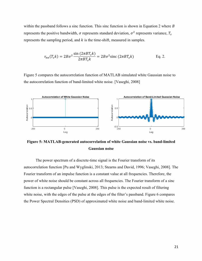
within the passband follows a sinc function. This sinc function is shown in Equation 2 where 𝐵
represents the positive bandwidth, 𝜎 represents standard deviation, 𝜎4 represents variance, 𝑇6
represents the sampling period, and 𝑘 is the time-shift, measured in samples.
𝑟99 𝑇6𝑘 = 2𝐵𝜎4sin (2𝜋𝐵𝑇6𝑘)2𝜋𝐵𝑇6𝑘
= 2𝐵𝜎4sinc (2𝜋𝐵𝑇6𝑘) Eq. 2.
Figure 5 compares the autocorrelation function of MATLAB simulated white Gaussian noise to
the autocorrelation function of band-limited white noise. [Vaseghi, 2008]
Figure 5: MATLAB-generated autocorrelation of white Gaussian noise vs. band-limited
Gaussian noise
The power spectrum of a discrete-time signal is the Fourier transform of its
autocorrelation function [Pu and Wyglinski, 2013; Stearns and David, 1996; Vaseghi, 2008]. The
Fourier transform of an impulse function is a constant value at all frequencies. Therefore, the
power of white noise should be constant across all frequencies. The Fourier transform of a sinc
function is a rectangular pulse [Vaseghi, 2008]. This pulse is the expected result of filtering
white noise, with the edges of the pulse at the edges of the filter’s passband. Figure 6 compares
the Power Spectral Densities (PSD) of approximated white noise and band-limited white noise.
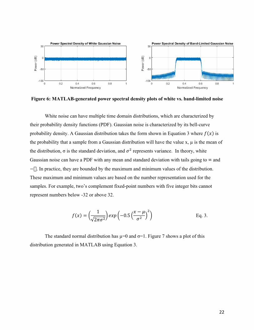
22
Figure 6: MATLAB-generated power spectral density plots of white vs. band-limited noise
White noise can have multiple time domain distributions, which are characterized by
their probability density functions (PDF). Gaussian noise is characterized by its bell-curve
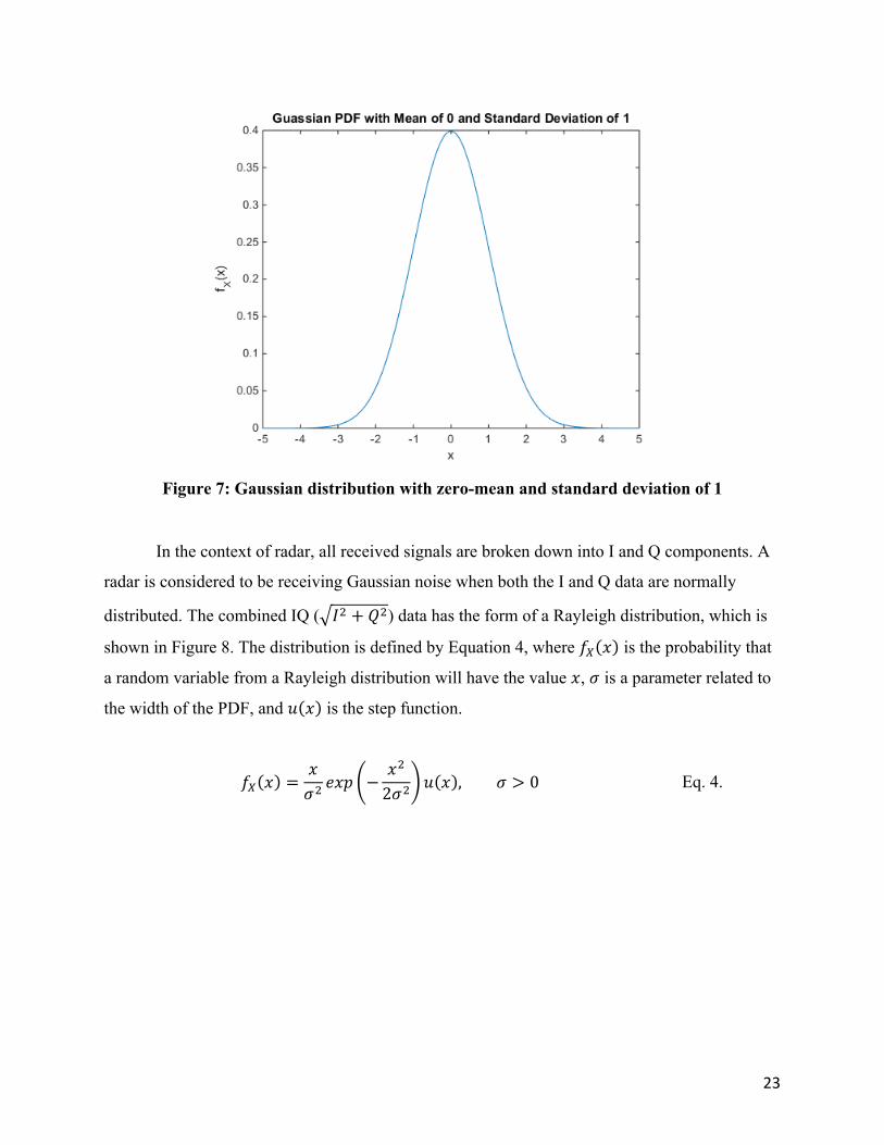
probability density. A Gaussian distribution takes the form shown in Equation 3 where 𝑓 𝑥 is
the probability that a sample from a Gaussian distribution will have the value x, µ is the mean of
the distribution, σ is the standard deviation, and 𝜎4 represents variance. In theory, white
Gaussian noise can have a PDF with any mean and standard deviation with tails going to ∞ and
−�. In practice, they are bounded by the maximum and minimum values of the distribution.
These maximum and minimum values are based on the number representation used for the
samples. For example, two’s complement fixed-point numbers with five integer bits cannot
represent numbers below -32 or above 32.
𝑓 𝑥 =12𝜋𝜎4
𝑒𝑥𝑝 −0.5𝑥 − 𝜇𝜎4
4 Eq. 3.
The standard normal distribution has µ=0 and σ=1. Figure 7 shows a plot of this
distribution generated in MATLAB using Equation 3.
23
Figure 7: Gaussian distribution with zero-mean and standard deviation of 1
In the context of radar, all received signals are broken down into I and Q components. A
radar is considered to be receiving Gaussian noise when both the I and Q data are normally
distributed. The combined IQ ( 𝐼4 + 𝑄4) data has the form of a Rayleigh distribution, which is
shown in Figure 8. The distribution is defined by Equation 4, where 𝑓M 𝑥 is the probability that
a random variable from a Rayleigh distribution will have the value 𝑥, 𝜎 is a parameter related to
the width of the PDF, and 𝑢 𝑥 is the step function.
𝑓M 𝑥 =𝑥𝜎4 𝑒𝑥𝑝 −
𝑥4
2𝜎4 𝑢 𝑥 , 𝜎 > 0 Eq. 4.
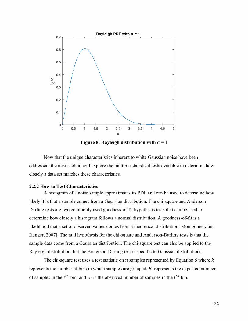
24
Figure 8: Rayleigh distribution with σ = 1
Now that the unique characteristics inherent to white Gaussian noise have been
addressed, the next section will explore the multiple statistical tests available to determine how
closely a data set matches these characteristics.
2.2.2 How to Test Characteristics A histogram of a noise sample approximates its PDF and can be used to determine how
likely it is that a sample comes from a Gaussian distribution. The chi-square and Anderson-
Darling tests are two commonly used goodness-of-fit hypothesis tests that can be used to
determine how closely a histogram follows a normal distribution. A goodness-of-fit is a
likelihood that a set of observed values comes from a theoretical distribution [Montgomery and
Runger, 2007]. The null hypothesis for the chi-square and Anderson-Darling tests is that the
sample data come from a Gaussian distribution. The chi-square test can also be applied to the
Rayleigh distribution, but the Anderson-Darling test is specific to Gaussian distributions.
The chi-square test uses a test statistic on 𝑛 samples represented by Equation 5 where 𝑘
represents the number of bins in which samples are grouped, 𝐸R represents the expected number
of samples in the 𝑖ST bin, and 𝑂R is the observed number of samples in the 𝑖ST bin.
25
𝑋W4 =(𝑂R − 𝐸R)4
𝐸R
X
RYZ
Eq. 5
The PDF of a chi-square distribution is defined in Equation 6 where 𝑘 − 𝑣 − 1 is the
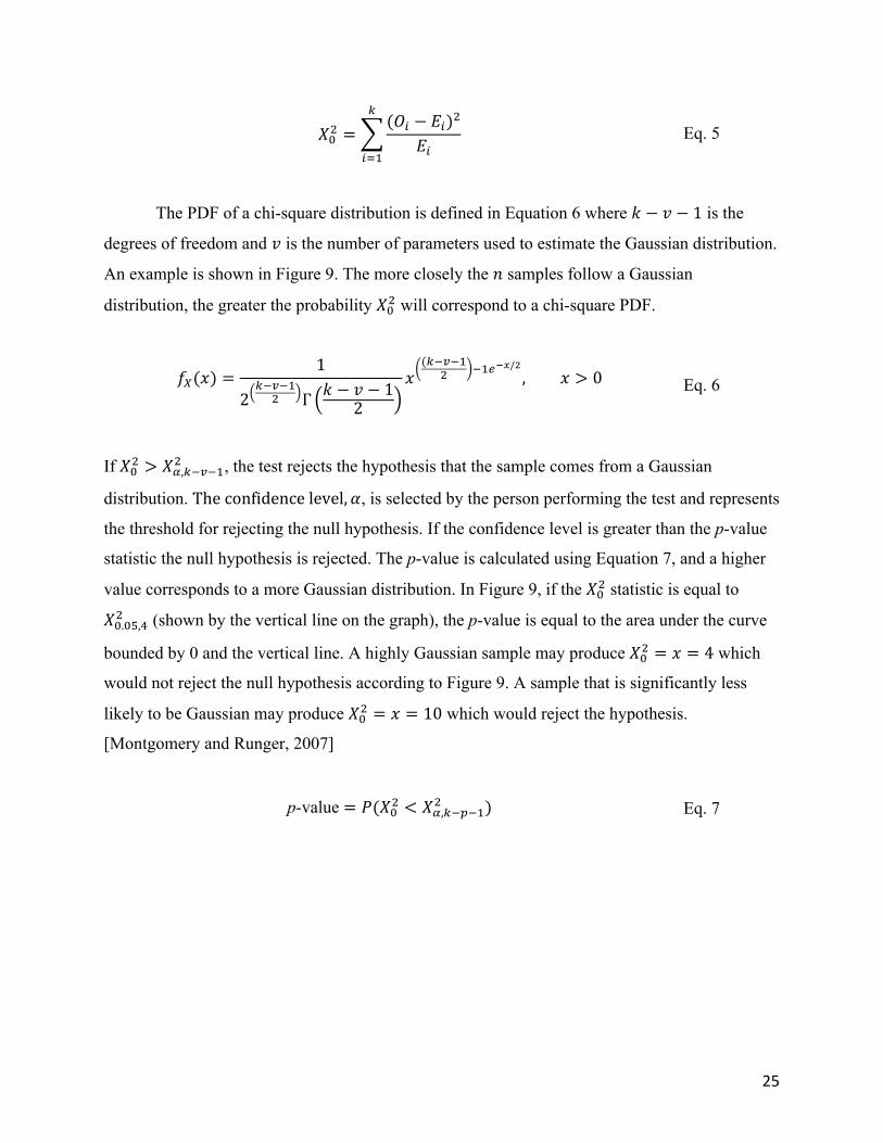
degrees of freedom and 𝑣 is the number of parameters used to estimate the Gaussian distribution.
An example is shown in Figure 9. The more closely the 𝑛 samples follow a Gaussian
distribution, the greater the probability 𝑋W4 will correspond to a chi-square PDF.
𝑓M(𝑥) =1
2X[\[Z
4 Γ 𝑘 − 𝑣 − 12
𝑥(X[\[Z
4 [Z^_`/b, 𝑥 > 0 Eq. 6
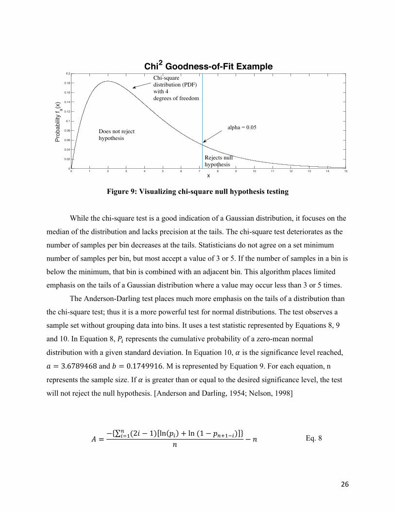
If 𝑋W4 > 𝑋c,X[\[Z4 , the test rejects the hypothesis that the sample comes from a Gaussian
distribution. The confidence level, 𝛼, is selected by the person performing the test and represents
the threshold for rejecting the null hypothesis. If the confidence level is greater than the p-value
statistic the null hypothesis is rejected. The p-value is calculated using Equation 7, and a higher
value corresponds to a more Gaussian distribution. In Figure 9, if the 𝑋W4 statistic is equal to
𝑋W.Wm,n4 (shown by the vertical line on the graph), the p-value is equal to the area under the curve
bounded by 0 and the vertical line. A highly Gaussian sample may produce 𝑋W4 = 𝑥 = 4 which
would not reject the null hypothesis according to Figure 9. A sample that is significantly less
likely to be Gaussian may produce 𝑋W4 = 𝑥 = 10 which would reject the hypothesis.
[Montgomery and Runger, 2007]
p-value = 𝑃(𝑋W4 < 𝑋c,X[r[Z4 ) Eq. 7
26
Figure 9: Visualizing chi-square null hypothesis testing
While the chi-square test is a good indication of a Gaussian distribution, it focuses on the
median of the distribution and lacks precision at the tails. The chi-square test deteriorates as the
number of samples per bin decreases at the tails. Statisticians do not agree on a set minimum
number of samples per bin, but most accept a value of 3 or 5. If the number of samples in a bin is
below the minimum, that bin is combined with an adjacent bin. This algorithm places limited
emphasis on the tails of a Gaussian distribution where a value may occur less than 3 or 5 times.
The Anderson-Darling test places much more emphasis on the tails of a distribution than
the chi-square test; thus it is a more powerful test for normal distributions. The test observes a
sample set without grouping data into bins. It uses a test statistic represented by Equations 8, 9
and 10. In Equation 8, 𝑃R represents the cumulative probability of a zero-mean normal
distribution with a given standard deviation. In Equation 10, 𝛼 is the significance level reached,
𝑎 = 3.6789468 and 𝑏 = 0.1749916. M is represented by Equation 9. For each equation, n
represents the sample size. If 𝛼 is greater than or equal to the desired significance level, the test
will not reject the null hypothesis. [Anderson and Darling, 1954; Nelson, 1998]
𝐴 =− (2𝑖 − 1) ln 𝑝R + ln (1 − 𝑝9zZ[R)9
RYZ
𝑛 − 𝑛 Eq. 8
x0 1 2 3 4 5 6 7 8 9 10 11 12 13 14 15
Prob
abilit
y f x(x
)
0
0.02
0.04
0.06
0.08
0.1
0.12
0.14
0.16
0.18
0.2Chi2 Goodness-of-Fit Example
Rejects nullhypothesis
Chi-squaredistribution (PDF)with 4degrees of freedom
Does not rejecthypothesis
alpha = .005alpha = 0.05
27
𝑀 = 𝐴 1 + . 75 𝑛 + 2.25 𝑛4 Eq. 9
𝛼 = 𝑎𝑒[| } Eq. 10
A limitation for both the Anderson-Darling and chi-square tests is sample size. Both test
outcomes are partially dependent on the size of the sample data set being analyzed. If two
samples of different size 𝑛 from the same set of data are analyzed using the same test, the results
will differ. Additionally, if the sample size is very small, it may not contain enough information
to accurately represent its distribution. Conversely, since a true Gaussian distribution is purely
theoretical, the tests will always fail if the sample set is large enough.
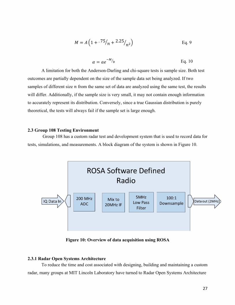
2.3 Group 108 Testing Environment Group 108 has a custom radar test and development system that is used to record data for
tests, simulations, and measurements. A block diagram of the system is shown in Figure 10.
Figure 10: Overview of data acquisition using ROSA
2.3.1 Radar Open Systems Architecture To reduce the time and cost associated with designing, building and maintaining a custom
radar, many groups at MIT Lincoln Laboratory have turned to Radar Open Systems Architecture
28
(ROSA). ROSA systems use subsystem components that meet standardized interfaces and are
easily replaceable for upgrades or repairs [Rejto, 2000]. Group 108 has a software-defined
ROSA system that the group uses for lab testing radar-related equipment. In the development
system in Building 1718, The ROSA system samples data input to the system as analog data over
a cable.
2.3.2 Existing Noise Sources in Group 108 One piece of equipment that currently can be tested in conjunction with the ROSA
system is the WhiteBox Lite DRFM. DRFMs receive a signal, digitize it at IF using the
conversion process described in Section 2.1.2, and retransmit the signal after a delay. Due to the
digital nature of the system, the signal can be delayed for an arbitrary period of time, and it can
be processed to change the amplitude or frequency [Wiegand et al., 1989]. Group 108 built and
uses a custom DRFM called WhiteBox Lite. WhiteBox Lite is primarily used as a target
generator for radar systems that the group builds and operates. The created targets may be either
single targets or repeated targets that can be used for jamming. It is also capable of creating noise
in the form of a frequency sweep, starting at a low frequency and moving towards a high
frequency at a user-specified rate and bandwidth. To receivers that integrate received signals
over time, this sweep is interpreted as noise over the given frequency band. However, noise
generated by a frequency sweep is completely deterministic. Currently, WhiteBox Lite has no
way to create unstructured Gaussian noise [Massa, 2015].
In addition to WhiteBox Lite, Group 108 has analog NoiseCom NC6108A noise
generators, which generate broadband Gaussian noise. These types of generators are designed to
produce truly random, unstructured noise, but making them configurable requires additional
analog hardware. Digital noise generators can be configurable by utilizing digital logic on
FPGAs. Group 108 is interested in having a configurable, standalone digital noise generation
device on an FPGA platform.
2.4 Digital Generation of Gaussian Noise Digitally generated Gaussian noise is created by converting normally distributed, pseudo-
random digital numbers to an analog signal. The resulting analog noise is always band-limited
due to hardware limitations such as sample rate and clock speed. Theoretical white Gaussian
noise would require a clock speed and a digital-to-analog converter (DAC) sample rate of
29
infinity. Previous works show that a number of algorithms for generating normally distributed
random numbers can be implemented on FPGAs.
2.4.2 Pseudorandom Number Generation Most of the following methods perform a series of calculations on a uniformly distributed
sample. Samples from a uniform distribution have an equal probability of being any number
between two endpoints (typically 0 and 1) [Pu and Wyglinski, 2013]. Pseudo-random uniform
numbers are relatively easy to generate on FPGAs using linear feedback shift registers (LFSRs).
In digital circuitry, a shift register is a cascade of flip-flops where each flip-flop transfers its
output value to the following flip-flop at every clock cycle. The initial value of the shift register
is called the seed. The value of a flip-flop that has shifted its value out is ‘0’ unless it receives a
value of ‘1’. If the number of shifts exceeds the number of flip-flops, every flip-flop will hold a
value of ‘0’. Linear feedback is a method of reintroducing logical ‘1’ values back into the shift
register, effectively increasing the register’s cycle. The feedback uses a logical operation, usually
exclusive-or, of several flip-flops in the shift register to set the value of the first flip-flop in the
cascade.
Once the uniformly distributed random numbers are produced there are a number of
different techniques to transform them to normally distributed numbers. The following sections
describe how various Gaussian random algorithms are implemented using programmable logic.
2.4.3 Techniques for Digitally Generating Gaussian Distributions Inverse Cumulative Density Function
A cumulative distribution function (CDF) represents the probability for every x that a
random number will have a value less than or equal to x. Since the range of standard uniform
random variables extends from 0 to 1, the CDF is essentially a mapping from a normal to a
uniform distribution. An inverse cumulative distribution function (ICDF) works the other way,
mapping from a uniform to a normal distribution. The inversion method generates a normal
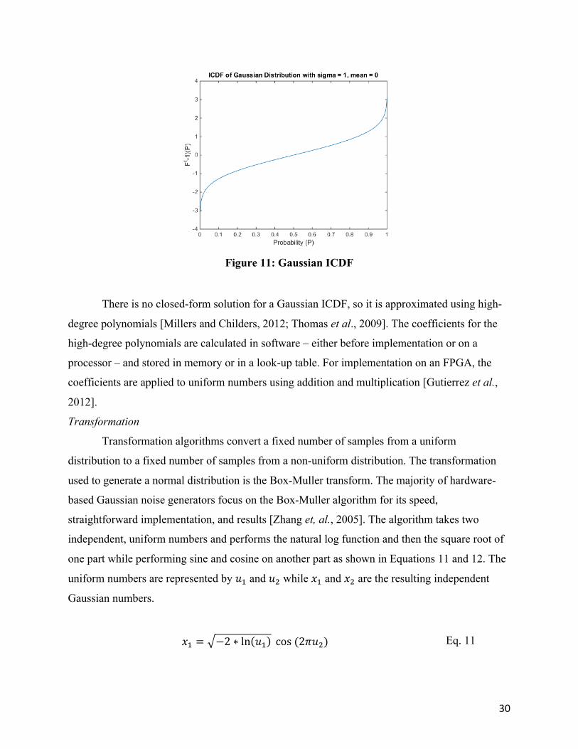
distribution by applying an ICDF to a uniform distribution. A plot of the ICDF is shown in
Figure 11.
30
Figure 11: Gaussian ICDF
There is no closed-form solution for a Gaussian ICDF, so it is approximated using high-
degree polynomials [Millers and Childers, 2012; Thomas et al., 2009]. The coefficients for the
high-degree polynomials are calculated in software – either before implementation or on a
processor – and stored in memory or in a look-up table. For implementation on an FPGA, the
coefficients are applied to uniform numbers using addition and multiplication [Gutierrez et al.,
2012].
Transformation
Transformation algorithms convert a fixed number of samples from a uniform
distribution to a fixed number of samples from a non-uniform distribution. The transformation
used to generate a normal distribution is the Box-Muller transform. The majority of hardware-
based Gaussian noise generators focus on the Box-Muller algorithm for its speed,
straightforward implementation, and results [Zhang et, al., 2005]. The algorithm takes two
independent, uniform numbers and performs the natural log function and then the square root of
one part while performing sine and cosine on another part as shown in Equations 11 and 12. The
uniform numbers are represented by 𝑢Z and 𝑢4 while 𝑥Z and 𝑥4 are the resulting independent
Gaussian numbers.
𝑥Z = −2 ∗ ln 𝑢Z cos (2𝜋𝑢4) Eq. 11

31
𝑥4 = −2 ∗ ln 𝑢Z sin (2𝜋𝑢4) Eq. 12
The minimum period of the Box-Muller transformation is the greatest period of the two
underlying uniform number generators. Using programmable logic, the Box-Muller transform
uses sine, cosine, log, and square root approximations. Coefficients for these operations can be
calculated and stored as described in the previous section.
Rejection
The Ziggurat algorithm is a popular method for generating Gaussian random numbers in
software. This algorithm will reject some uniform samples, instead moving on to use another
sample. This rejection of certain samples requires additional logic, so the method is not
guaranteed constant throughput. The inconstant throughput is trivial in software, but it is
undesirable in hardware because the DAC throughput is constant regardless of whether or not a
new sample has been produced [Lee et, al., 2005].
The algorithm is implemented by first determining a number of layers that define the
shape of the resulting curve. Visually, a plot of the layers resembles a step pyramid. More layers
result in higher resolution, and thus create a more statistically sound Gaussian output. First, one
of the layers is randomly selected using certain bits from a uniform number. The value of the
layer is multiplied by the uniform number. Logical if statements determine whether the results of
the multiplication are clearly within the curve of the distribution. In cases where the sample is
close to the curve, additional processing must be performed to determine whether the sample
should be accepted or rejected. This additional processing causes a stall and non-constant
throughput, and must be performed more often for a less precise approximation with less layers.
The tails of the distribution are filled from the bottom layer, which extends to infinity. This
processing is often done using natural log, division, and multiplication. Figure 12 shows a
resolution comparison between 4 layers and 16 layers [Lee et al., 2005].
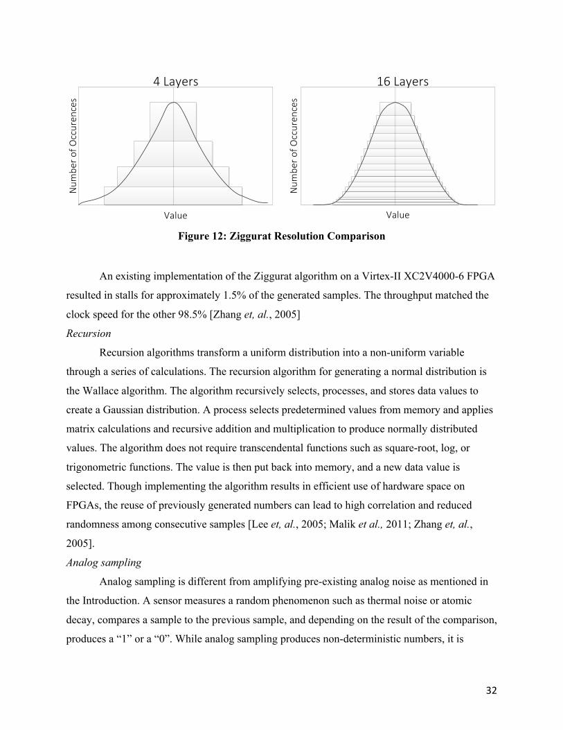
32
32-‐bit Tausworthe uniform random number generator
Coefficient ROM Delay Absolute Value
Comparator
FIFO2
Operation Unit
FIFO3
FIFO1
Multiplexer
18-‐bit
i32-‐bit
32-‐bit
18-‐bit
i
32-‐bit
36-‐bit
36-‐bit
REQ
36-‐bitMSB
Gaussian Out
8-‐bit
Value Value
Num
ber o
f Occuren
ces
Num
ber o
f Occuren
ces
4 Layers 16 Layers
Figure 12: Ziggurat Resolution Comparison
An existing implementation of the Ziggurat algorithm on a Virtex-II XC2V4000-6 FPGA
resulted in stalls for approximately 1.5% of the generated samples. The throughput matched the
clock speed for the other 98.5% [Zhang et, al., 2005]
Recursion
Recursion algorithms transform a uniform distribution into a non-uniform variable
through a series of calculations. The recursion algorithm for generating a normal distribution is
the Wallace algorithm. The algorithm recursively selects, processes, and stores data values to
create a Gaussian distribution. A process selects predetermined values from memory and applies
matrix calculations and recursive addition and multiplication to produce normally distributed
values. The algorithm does not require transcendental functions such as square-root, log, or
trigonometric functions. The value is then put back into memory, and a new data value is
selected. Though implementing the algorithm results in efficient use of hardware space on
FPGAs, the reuse of previously generated numbers can lead to high correlation and reduced
randomness among consecutive samples [Lee et, al., 2005; Malik et al., 2011; Zhang et, al.,
2005].
Analog sampling
Analog sampling is different from amplifying pre-existing analog noise as mentioned in
the Introduction. A sensor measures a random phenomenon such as thermal noise or atomic
decay, compares a sample to the previous sample, and depending on the result of the comparison,
produces a “1” or a “0”. While analog sampling produces non-deterministic numbers, it is

33
considerably slower than the previous algorithms mentioned. It can only produce one bit at a
time, so generating a single set of 16-bit IQ data requires 32 clock cycles. Prior art using this
method is directed towards cryptography where significantly more emphasis is placed on the
randomness of the number generators and less emphasis is placed on speed. [Drutarovsky et, al.,
2004; Callegari et, al., 2005]
Central Limit Theorem
The Central Limit Theorem states that means of random variables “converge to a
Gaussian random variable in distribution” [Miller and Childers, 2013]. To implement the central
limit theorem in conjunction with the aforementioned algorithms, sets of normally distributed
data are averaged before output. The convergence introduced by this technique can produce a
more Gaussian distribution than the distribution produced by an individual generator [Lee et, al.,
2005]. Implementing the Central Limit Theorem separately from other algorithms can also be
done by band pass filtering a uniform distribution to produce a more Gaussian distribution.
However, the samples are no longer independent or uncorrelated after filtering.
2.5 Digital Programmability Regardless of the algorithm used, digitally produced noise has an advantage over analog
noise in the form of its high programmability. The following section describes how the center
frequency, bandwidth, and amplitude can be digitally adjusted.
2.5.1 Center Frequency and Bandwidth One of the most common ways to select the desired frequency response of a system is to
use a filter. A filter is a device that passes signals at certain frequencies while attenuating others.
Band pass filters are designed with a specified center frequency and bandwidth. Filters can be
implemented using either analog or digital methods [Paul et al., 2015].
A digital filter works by determining a set of coefficients that, when multiplied by a
combination of past and present input and output values, generate a desired frequency response.
An ideal band pass filter would pass the desired frequencies and completely attenuate the
undesired frequencies. However, a filter implemented in real time must be causal, relying on
only values that occur between time zero and the present time, which imposes restrictions on the
frequency response characteristic. An ideal filter is not achievable in practice. Causal, linear
filters are described in Equation 13 where x is the input signal, y is the output signal, and {𝑎X}
34
and {𝑏X} are the coefficients. Since the filter designer is limited to causal systems for real
applications, the designer must properly select the coefficients {𝑎X} and {𝑏X} to design a system
that approximates the ideal frequency response characteristics [Proakis and Manolakis, 1996]
𝑦 𝑛 = 𝑏X𝑥(𝑛 − 𝑘)|
XYW− 𝑎X𝑦(𝑛 − 𝑘)
�
XYZ Eq. 13
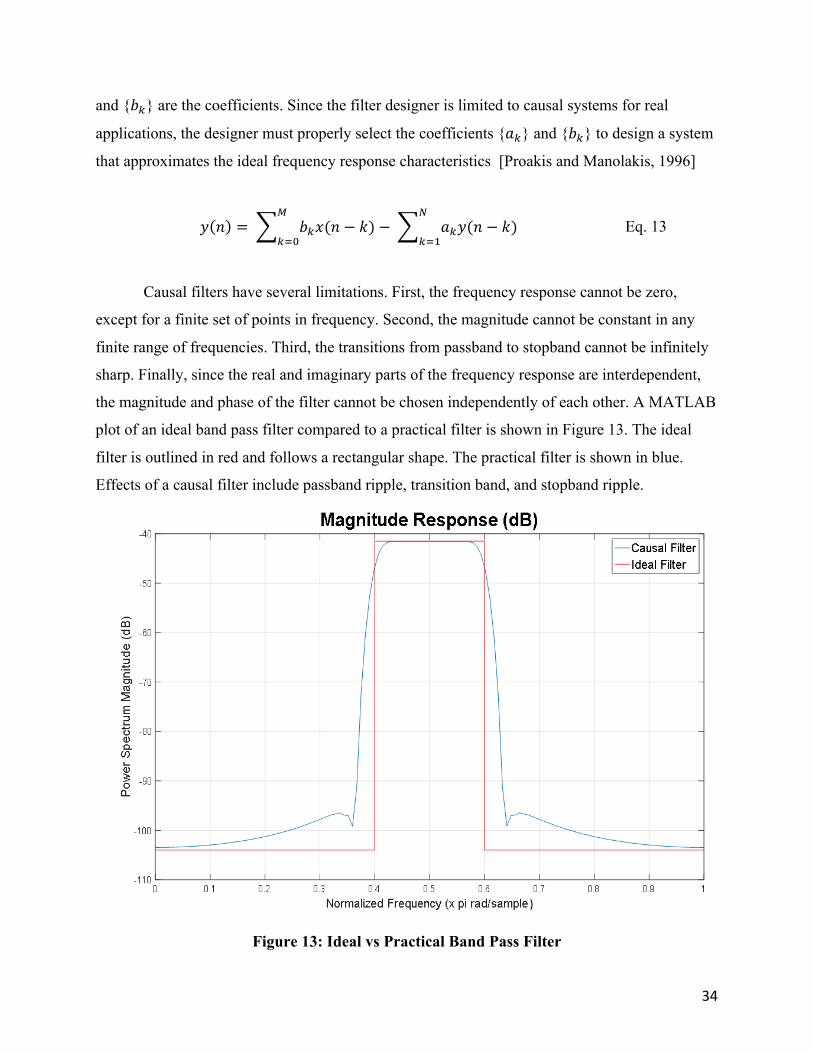
Causal filters have several limitations. First, the frequency response cannot be zero,
except for a finite set of points in frequency. Second, the magnitude cannot be constant in any
finite range of frequencies. Third, the transitions from passband to stopband cannot be infinitely
sharp. Finally, since the real and imaginary parts of the frequency response are interdependent,
the magnitude and phase of the filter cannot be chosen independently of each other. A MATLAB
plot of an ideal band pass filter compared to a practical filter is shown in Figure 13. The ideal
filter is outlined in red and follows a rectangular shape. The practical filter is shown in blue.
Effects of a causal filter include passband ripple, transition band, and stopband ripple.
Figure 13: Ideal vs Practical Band Pass Filter
35
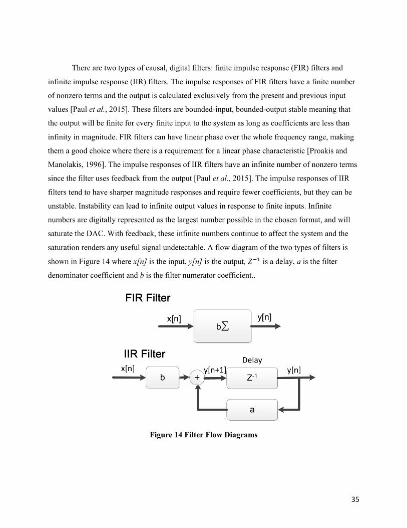
There are two types of causal, digital filters: finite impulse response (FIR) filters and
infinite impulse response (IIR) filters. The impulse responses of FIR filters have a finite number
of nonzero terms and the output is calculated exclusively from the present and previous input
values [Paul et al., 2015]. These filters are bounded-input, bounded-output stable meaning that
the output will be finite for every finite input to the system as long as coefficients are less than
infinity in magnitude. FIR filters can have linear phase over the whole frequency range, making
them a good choice where there is a requirement for a linear phase characteristic [Proakis and
Manolakis, 1996]. The impulse responses of IIR filters have an infinite number of nonzero terms
since the filter uses feedback from the output [Paul et al., 2015]. The impulse responses of IIR
filters tend to have sharper magnitude responses and require fewer coefficients, but they can be
unstable. Instability can lead to infinite output values in response to finite inputs. Infinite
numbers are digitally represented as the largest number possible in the chosen format, and will
saturate the DAC. With feedback, these infinite numbers continue to affect the system and the
saturation renders any useful signal undetectable. A flow diagram of the two types of filters is
shown in Figure 14 where x[n] is the input, y[n] is the output, 𝑍[Z is a delay, a is the filter
denominator coefficient and b is the filter numerator coefficient..
Figure 14 Filter Flow Diagrams
36
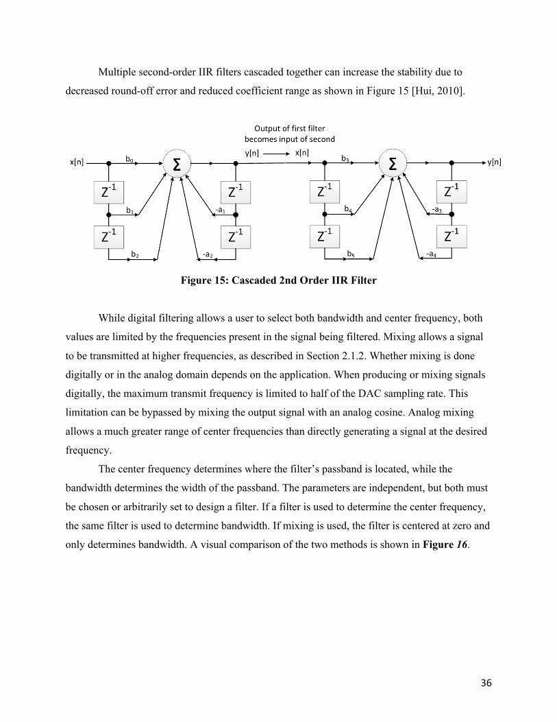
Multiple second-order IIR filters cascaded together can increase the stability due to
decreased round-off error and reduced coefficient range as shown in Figure 15 [Hui, 2010].
Figure 15: Cascaded 2nd Order IIR Filter
While digital filtering allows a user to select both bandwidth and center frequency, both
values are limited by the frequencies present in the signal being filtered. Mixing allows a signal
to be transmitted at higher frequencies, as described in Section 2.1.2. Whether mixing is done
digitally or in the analog domain depends on the application. When producing or mixing signals
digitally, the maximum transmit frequency is limited to half of the DAC sampling rate. This
limitation can be bypassed by mixing the output signal with an analog cosine. Analog mixing
allows a much greater range of center frequencies than directly generating a signal at the desired
frequency.
The center frequency determines where the filter’s passband is located, while the
bandwidth determines the width of the passband. The parameters are independent, but both must
be chosen or arbitrarily set to design a filter. If a filter is used to determine the center frequency,
the same filter is used to determine bandwidth. If mixing is used, the filter is centered at zero and
only determines bandwidth. A visual comparison of the two methods is shown in Figure 16.

37
Figure 16: Broadband vs. Baseband Generation
2.5.2 Amplitude In addition to center frequency and bandwidth, the amplitude of a signal can be configured.
Adjusting the amplitude can be done using analog components or digital logic. Amplifiers can be
used to attenuate or amplify the analog output of a digitally generated signal, but require external
hardware. If the signal is modified digitally, the output amplitude is related to the magnitude of
the digital values and the power that the DAC can output. The method for controlling the
amplitude in logic is multiplying the signal by a constant. This multiplication allows easy control
of the final signal power by reducing the maximum output [Bird, 2007]. A signal can be
attenuated without modifying logic values by reducing the maximum voltage used by the DAC.
Group 108 currently has capabilities for testing false target jamming and broadband, analog
noise jamming; however, they do not currently have a method for digital, configurable, Gaussian
noise jamming. The next section will detail the methods used to design and implement a
standalone platform for the Group’s test and development system to meet this need.

38
3.0 Methods
This chapter details our methodology for designing a digital, programmable, band-limited,
white Gaussian noise generator on the Xilinx Kintex-7 Digital Signal Processing Development
Kit (KC705). Section 3.1 introduces our project requirements. Section 3.2 explains our platform
decision. Section 3.3 covers our algorithm selection. Section 3.4 follows our implementation.
3.1 Project Requirements At the beginning of the project, Group 108 defined a set of explicit requirements for our
generator. First, the generator needed to be implemented on a standalone hardware platform with
a Xilinx FPGA in order to be integrated with the existing DRFM jammer of the group, WhiteBox
Lite, in the future. Second, the platform had to be capable of transmitting at 20 MHz to match the
frequency at which the ROSA system operates. Third, noise produced by the generator needed to
have user programmable amplitude, center frequency, and bandwidth. Last, the noise generator
needed to be capable of interfacing with WhiteBox Lite by transmitting IQ data through both
analog cable and Ethernet. The group requires that both the I and Q data be Gaussian and
independent. ROSA reads the I and Q data separately, then combines the two signals as part of
its digital processing. A high-level block diagram showing how the noise generator will integrate
with the current test and development system is shown in Figure 17. In addition to the given
project requirements, we developed a test suite for Gaussian noise that our results must pass, as
described in the following section.
39
Figure 17: High Level Integration Diagram 3.2 Gaussian Test Suite
We developed a test suite for Gaussian noise based on the characteristics of Gaussian noise
described in Section 2.3. The test suite consists of three visual inspections and two statistical
tests based on a sample data set’s PDF, autocorrelation, and power spectrum.
The test suite uses MATLAB to generate plots of the estimated PDF in the form of a
histogram, autocorrelation, and frequency spectrum of a sample data set. First, we examine the
histograms of the I and Q noise for a symmetrical, bell-shaped curve centered at zero and the
histogram of the combined IQ data for a Rayleigh distribution. Second, we examine the
autocorrelation for a sinc function. Last, we examine the power spectrum for a flat spectrum
within the desired bandwidth. These visual inspections are supported by two statistical tests.
The two statistical tests used were the chi-square and Anderson-Darling goodness-of-fit tests
based on the histograms of the sample data I and Q and the combined IQ data. We used the
existing MATLAB 2014b functions chi2gof (chi-square) and adtest (Anderson-Darling) with the
null hypothesis that the sample I and Q data came from a normal distribution. We also ran the
chi2gof test with the null hypothesis that the combined IQ data came from a Rayleigh
distribution. The Anderson-Darling test cannot be applied to Rayleigh distributions. Both
MATLAB functions return a p-value and a test decision on the null hypothesis based on a user-
specified significance level. While we were in the process of developing the test suite, we also
selected the hardware platform for our project.
3.3 Hardware Selection We researched and compared eight potential hardware platforms that were either
recommended to us by Group 108 or that we discovered through online research. We compared
each platform’s price, RF range, DAC resolution and range, and number of logic cells available.
The requirements of a Xilinx FPGA and ability to transmit at 20 MHz eliminated six of the eight
options. A full value analysis is in Appendix A. The remaining platforms were the Ettus
Research X310 USRP (Ettus), a software defined radio, and the Xilinx Kintex-7 Digital Signal
Processing Development Kit (KC705). Both platforms have a 16-bit, dual-channel DAC with a
maximum sample rate of 800 megasamples per second (Ms/s), a Xilinx Kintex-7 FPGA, analog
output, and an Ethernet port. We chose to use both platforms for our project for several reasons.
40
We worked with the KC705 first because we had immediate access while there was significant
lead time for the Ettus. Furthermore, the KC705 is the current hardware of WhiteBox Lite and
the source code was available to us. We planned to use the Ettus for our final design because the
hardware is already fully encased while the KC705 requires an expensive, custom-built case.
However, due to unforeseen complications, we were unable to complete our implementation on
the Ettus and instead used the KC705 as our final platform. The following sections detail our
work with the KC705.
3.4 Implementation The KC705 is a development kit consisting of a development board with a high-powered
Kintex-7 XC7K325T FPGA and a signal processing daughter card with dual-channel, 14-bit
ADC and 16-bit DAC. The KC705 is the platform currently used for WhiteBox Lite. This board
has multiple features which were significant for our application: it has over 325,000 logic cells,
which are the basic unit of the FPGA and consist of a flip-flop, a lookup table to implement
combinational logic, and connections to other cells. It also has 840 DSP slices, which combine a
fixed-point multiplier and accumulator, and can be used to increase the speed at which
mathematical operations are performed. Finally, the development board has flash memory, which
can be used to store a project design and program the design to the FPGA at runtime. While the
DAC is capable of a maximum sample rate of 800 megasamples per second (Ms/s), it is
configured to run at 250 Ms/s on WhiteBox Lite. This rate matches the system clock speed of
250 MHz, which is the fastest the clock can run without timing issues caused by the clock signals
reaching different parts of the board at different times. As we used a significant amount of the
existing WhiteBox Lite architecture, we chose to keep this DAC sample rate and system clock
speed. The following sections detail how we implemented a digital, programmable, Gaussian
noise generator on the KC705.
3.4.1 Random Number Algorithm Selection and Implementation
For the KC705, we needed a normally distributed random number generation algorithm
with characteristics that would make it suitable for generating noise on an FPGA platform, as
described in Section 2.4. We ruled out the rejection and recursion methods due to non-constant
throughput, the analog sampling method due to slow throughput, the Central Limit Theorem due
41
to limited frequency range, and the inversion method due to the large number of coefficients
required. We selected the Box-Muller transformation algorithm for its speed, constant output
rate, and ability to generate high-quality noise. This algorithm transforms two, independent
uniform, numbers into two, independent, normal numbers. We used the two normally distributed
numbers as the I and Q data for the output. The transformation is shown in Equation 14, where
𝑢Z and 𝑢4 are the unform numbers, and 𝑥Z and 𝑥4 are the normal numbers.
𝑥Z = −2 ∗ ln 𝑢Z cos (2𝜋𝑢4) Eq. 14a
𝑥4 = −2 ∗ ln 𝑢Z sin (2𝜋𝑢4) Eq. 14b
We modeled our initial algorithm design on prior art published in IEEE Transactions on
Computers that discussed a general method for hardware implementation of the Box-Muller
algorithm [Lee et al., 2006]. The considerations of the paper included the necessary sample bit
length and how to implement functions such as square roots, logarithms and trigonometric
functions in hardware. The authors represented 𝑥Zand 𝑥4 with 16 bits to match the width of their
DAC. Five of these bits form the integer portion of the number, allowing the tails to extend to
approximately 8.1 standard deviations from the mean. Their error analysis for each step of the
process showed strong statistical results when 𝑢Z was represented by 48 bits and 𝑢4 represented
by 16 bits. In a fixed-point uniform number, each bit has an equal probability of having a value
of ‘0’ or ‘1’. Therefore, bits from uniform numbers can be separated and concatenated at will,
and the resulting number will still be uniform. The numbers 𝑢Z and 𝑢4 can then be produced by
taking bits from two 32-bit uniform numbers. To perform transcendental functions, the authors
scaled the values at each stage to a certain range and then divided the range into a number of
segments. Each segment was linearly approximated using a set of polynomials and coefficients.
To begin the implementation of our algorithm, we had to choose a method for generating
uniform random numbers. The period of the Box-Muller algorithm matches that of its input. As
discussed previously, using an LFSR is a fast method for generating uniform, fixed-point
numbers of a certain bit length. However, a 32-bit LFSR only has a maximum period of 232. At a
rate of 250 Ms/s, the uniform numbers would begin to repeat after just 17 seconds, which could
lead to noise that repeats within the same test.

42
A solution is the Tausworthe algorithm, which utilizes modulo 2 math based on three
parameters called k, q, and s. The Tausworthe is implemented in digital logic using the steps
below where A, B, and C are three binary vectors. C is a fixed vector, while A and B both
change on every iteration. A and B are seeded with initial values at the start of the algorithm
using logic. The final value of A at step 6 is taken as the output uniform number. The cycle then
repeats with the new values of A and B.
Step 1. B ← q-bit left-shift of A
Step 2. B ← A ⊕ B
Step 3. B ← k-bit right-shift of B
Step 4. A ← A&C
Step 5. A ← s-bit left-shift of A
Step 6. A ← A ⊕ B
Maximally equidistributed and combined (MEC) Tausworthe uniform number generators
have statistically more random output than single Tausworthes. An MEC Tausworthe is created
by implementing multiple Tausworthe algorithms with different values for C, k, q, s, and the
seed, and applying exclusive-or to each bit of all three outputs. We chose to use an MEC 32-bit
Tausworthe uniform number generator combining three Tausworthes to achieve a maximum
period of 288. A period of 288 does not repeat for over 39 billion years at our sampling rate, which
is sufficiently long for any possible test. The first Tausworthe uses 19, 13, and 12 for k, q, and s,
respectively. The second Tausworthe uses 25, 2, and 4. The third Tausworthe uses 11, 3, and 17.
The final result is the exclusive-or of all three individual Tausworthe outputs. Each bit has a 50%
chance of being a ‘1’ or a ‘0’; thus, every possible output is equally likely, which makes the
output uniform. Many previous works in random number generation on FPGAs use the
aforementioned combination for uniform number generation. [L’Ecuyer, 1996].
We implemented two MEC Tausworthe modules to generate 𝑢Z and 𝑢4. The two
Tausworthes are seeded differently to ensure that they are independent of each other. The first
seeds A1 and C1 with 0xFFFFFFFF and 0xFFFFFFFE, A2 and C2 with 0xCCCCCCCC and
0xFFFFFFF8, and A3 and C3 with 0x00FF00FF and 0xFFFFFFF0. The second Tausworthe
seeds A1, A2, and A3 with 0x1F1F1F1F, 0xAACCAACC, and 0x55555555 respectively while

43
C1, C2, and C3 remain the same. For both modules, B is assigned at the first step rather than
independently seeded. Next, we developed our method for transforming the uniformly
distributed numbers to normally distributed numbers. Initially, we used fixed-point calculations
and approximations, but later we added floating point math.
Implementation 1: Fixed-Point Math and Polynomial Approximations
To approximate the transcendental functions in the Box-Muller algorithm, we determined
polynomial coefficients using MATLAB. For the logarithm and square root operations, the
transformed number is scaled by removing the leading zeroes and assuming a number of integer
bits that would place the number in the range for which coefficients were calculated. This
procedure is equivalent to representing the number in binary scientific notation. The first bits
after the leading zeros would be used to place the number into one of the predetermined
segments and decide which coefficients to use to approximate the value. After calculating the
value, the numbers were re-scaled using the equivalencies shown in Equations 15 and 16, where
𝑀� is the mantissa, which is in [1, 2), and 𝐸� is the binary exponent.
ln (𝑀� ∗ 2�`) = ln 𝑀� + 𝐸� ∗ ln (2) Eq. 15
𝑀� ∗ 2�` = 𝑀� ∗ 2�`b (even 𝐸�) Eq. 16a
𝑀� ∗ 2�` = 2 ∗ 𝑀� ∗ 2�`_�b (odd 𝐸�) Eq. 16b
The logarithm range was divided into 256 segments, each defined by three coefficients.
The log function was applied to a 48-bit number consisting of 32 bits from one Tausworthe and
16 bits from the other. Since the output of the Tausworthes are uniform and independent, all bit
combinations are equally likely; thus, they are still uniform. The log coefficients were
represented by 48 bits to match the length of the input. The result is truncated to 7 integer bits
and 24 fractional bits and these 31 most significant bits are carried over to the next stage. The
square root function was applied to the 31-bit result of the log function. The square root had two
separate sets of 64 coefficients based on whether the exponent of the number in binary scientific
notation was even or odd, as shown in Equation 16. Again, the coefficients were represented by
31 bits to match the square root input length. The result is represented using 4 integer bits and 13
fractional bits, for a total of 17 bits.
44
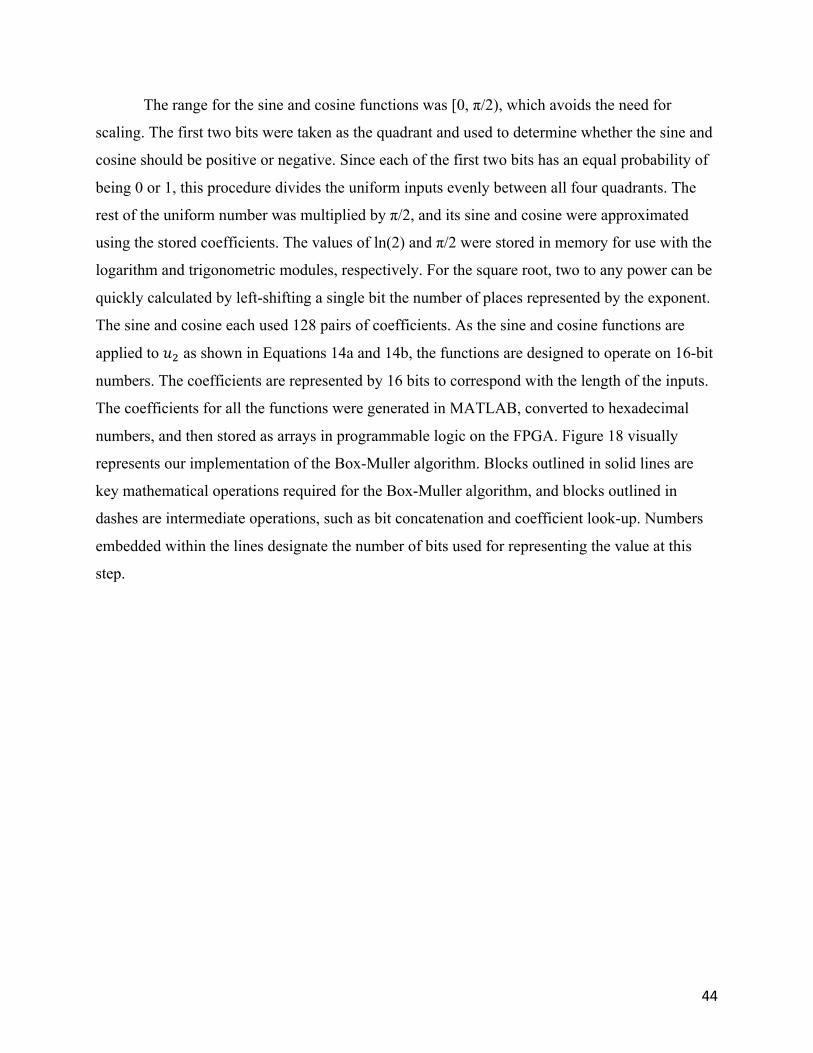
The range for the sine and cosine functions was [0, π/2), which avoids the need for
scaling. The first two bits were taken as the quadrant and used to determine whether the sine and
cosine should be positive or negative. Since each of the first two bits has an equal probability of
being 0 or 1, this procedure divides the uniform inputs evenly between all four quadrants. The
rest of the uniform number was multiplied by π/2, and its sine and cosine were approximated
using the stored coefficients. The values of ln(2) and π/2 were stored in memory for use with the
logarithm and trigonometric modules, respectively. For the square root, two to any power can be
quickly calculated by left-shifting a single bit the number of places represented by the exponent.
The sine and cosine each used 128 pairs of coefficients. As the sine and cosine functions are
applied to 𝑢4 as shown in Equations 14a and 14b, the functions are designed to operate on 16-bit
numbers. The coefficients are represented by 16 bits to correspond with the length of the inputs.
The coefficients for all the functions were generated in MATLAB, converted to hexadecimal
numbers, and then stored as arrays in programmable logic on the FPGA. Figure 18 visually
represents our implementation of the Box-Muller algorithm. Blocks outlined in solid lines are
key mathematical operations required for the Box-Muller algorithm, and blocks outlined in
dashes are intermediate operations, such as bit concatenation and coefficient look-up. Numbers
embedded within the lines designate the number of bits used for representing the value at this
step.

45
Figure 18: Diagram of Fixed-Point Box-Muller Algorithm Implementation
Implementation 2: Floating-Point Math and Look-Up Tables
To improve our throughput as well as to potentially increase the statistical quality of the
output noise, we added floating point math and look-up tables to our algorithm. We used
intellectual property (IP) provided by Xilinx, which can be fully pipelined to ensure maximum
throughput.
While fixed-point operations are intuitive in hardware, they lack the precision of floating-
point math. Integers represented by 32 fixed bits can represent numbers ranging from −2�Z to
2�Z − 1 while 32-bit floating-point can represent numbers ranging from approximately
±1.18 × 10[�� to ±3.4 × 10��. Floating-point math is often avoided on FPGAs due to the
complex operations needed to perform even the most basic calculations and the high logic
utilization. We addressed the first issue by using fully pipelined computation modules provided
by Xilinx through the IP CoreGen user interface, which produce one output value per clock
TauswortheUniform Random
Number Generator 1
TauswortheUniform Random
Number Generator 2
ConcatenateMultiply by pi/2
Natural LogCoefficient Look-‐Up
Multiply by -‐2
Square Root
Multiply by CosineMultiply by Sine
32 1614
48
31
31
14
16
16
31 31
16-‐bit In-‐Phase Data Out
16-‐bit Quadrature Data
Out
16 16
Sine
16
Cosine
16
Coefficient Look-‐Up 48
Coefficient Look-‐Up 31
QuadrantDetermines Sign
of Result
2

46
cycle. We chose to use existing modules instead of creating our own to save time and for their
ease of use. The modules include conversions between floating and fixed-point numbers, a
square root function, addition and subtraction, multiplication, a natural logarithm function, and
the sine and cosine functions. A diagram of the progression through the modules is shown in
Figure 19. Blocks outlined in solid lines are key mathematical operations required for the Box-
Muller algorithm, and blocks outlined in dashes are intermediate operations such as conversion
between floating and fixed point number representations. Numbers embedded within the lines
designate the number of bits used for representing the value at this step.
TauswortheUniform Random
Number Generator 1
TauswortheUniform Random
Number Generator 2
ConcatenateMultiply by pi
To Single Precision Float
To Single Precision Float
Natural Log
Look-‐Up Table
Multiply by -‐2
Square RootTo Single
Precision Float
Multiply by CosineMultiply by Sine
32 1616
56
32
32
32
16
16 16
32
32 3232
32 32
To Integer To Integer
16-‐bit In-‐Phase Data Out
16-‐bit Quadrature Data
Out
16 16
Fixed-‐Point
Floating Point
Fixed-‐Point
Fixed-‐Point
Floating Point
Fixed-‐Point
Sine
16
Cosine
16
zeros 8
Figure 19: Block Diagram of Second Box-Muller Implementation

47
The left side of the block diagram in Figure 19 illustrates the calculation of −2ln (𝑥4)
from the Box-Muller algorithm represented by equations 14a and 14b. Since 𝑥4 is intended to be
a uniform number between 0 and 1, we chose to use all 48 bits to represent the decimal. We then
convert the fixed point number to a single precision, floating-point number using a module
provided by Xilinx. The module expects the input to represent the integer with 8 bits and the
decimal with 48 bits, so we concatenated 8 zeros to the most significant bit of each 48-bit
number. The resulting 32-bit float then goes to a floating point module that performs the natural
log. The result of the natural log is multiplied by a constant of -2 in floating-point representation.
The square root of the multiplication result is then taken in floating-point.
The right side of the block diagram represents the sin (𝑢4) and cos (𝑢4) from equations
14a and 14b. To produce sine and cosine values, we tried two methods: the CORDIC module as
well as a sine and cosine look-up table, which are both provided by Xilinx. The CORDIC
algorithm is a method for calculating trigonometric functions without multiplication by using bit
shifting, look-up-tables, addition, and subtraction. The look-up table matches input values to
output values stored in logic. Both methods expect a fixed-point input between 𝜋 and – 𝜋
represented by 1 sign bit, 2 integer bits, and 13 bits for the decimal. To produce values within
this range, we multiply 16 bits from one of the Tausworthe generators by a fixed-point
representation of 𝜋 using Xilinx’s fixed-point multiplication module. The uniform input is
represented by 1 sign bit and 15 decimal bits, while 𝜋 and the output are represented by 1 sign
bit, 2 integer bits, and 13 bits for the decimal. Multiplication with these representations is
equivalent to multiplying a range of -1 to 1 by 𝜋 to get a range of −𝜋 to 𝜋. The sine and cosine
outputs are also fixed point and range from -1 to 1 represented by 1 sign bit, 1 integer bit, and 14
bits for the decimal. We then converted the fixed point outputs to single precision floating point
numbers. We produce I and Q data respectively by multiplying the 32-bit floats representing
cosine and sine by the floating point result from the square root module. We then convert the I
and Q numbers back to fixed point numbers to be sent to the DAC. Testing showed that the look-
up table was significantly more effective than the CORDIC module.
Using this algorithm with our chosen number representations, the largest number we can
represent with our fixed point output is approximately 8.16, which was calculated using Equation
20.

48
𝑀𝐴𝑋 = −2ln (2[n�) ∗ cos 2[Zn ≡ 8.16 Eq. 20
Based on our maximum output value, we chose to represent our final output using 1 bit
for the sign, 4 bits for the integer, and the remaining 11 bits for the decimal; however, further
investigation showed that the greatest number being output was approximately 3.5, and thus the
smallest number that the 48-bit vector was representing was around 2[�. This low number is due
to the way that the second Tausworthe is seeded. The final output was changed so that 1 bit was
used for the sign, 2 for the integer, and 13 for the decimal. We were satisfied with our statistical
results, and did not change the seeding.
The method for converting random numbers to noise signals remained almost unchanged.
The DAC is capable of converting both I and Q data at a frequency of 250MHz, outputting
frequencies up to 125MHz. Since floating-point numbers are more precise than fixed-point with
no penalty in speed, we chose the floating-point implementation for our final noise generator.
3.4.2 Programmability
Once we implemented a normally distributed random number generator, we focused on a
method for making the noise amplitude, bandwidth and center frequency programmable. The
methods used to manipulate our output were implemented on the KC705 FPGA while the ability
to select parameters for these methods was implemented on a soft processor. The processor is a
modified version of the WhiteBox Lite processor generated using FPGA logic.
Determining Center Frequency and Bandwidth The two options for controlling the center frequency characteristics of the noise generator
are generating directly at the desired center frequency and mixing baseband noise to higher
frequencies. The bandwidth is determined by a filter regardless of the method chosen. The
KC705 does not contain any analog signal processing hardware, so any frequency control must
be performed digitally. This limitation means that the center frequency and bandwidth are
constrained by the clock speed of 250 MHz. The Nyquist frequency is half of that rate, or
approximately 125 MHz. Since the Box-Muller algorithm produces a value at every clock cycle,
the KC705 can directly generate frequencies between 0 and 125 MHz.
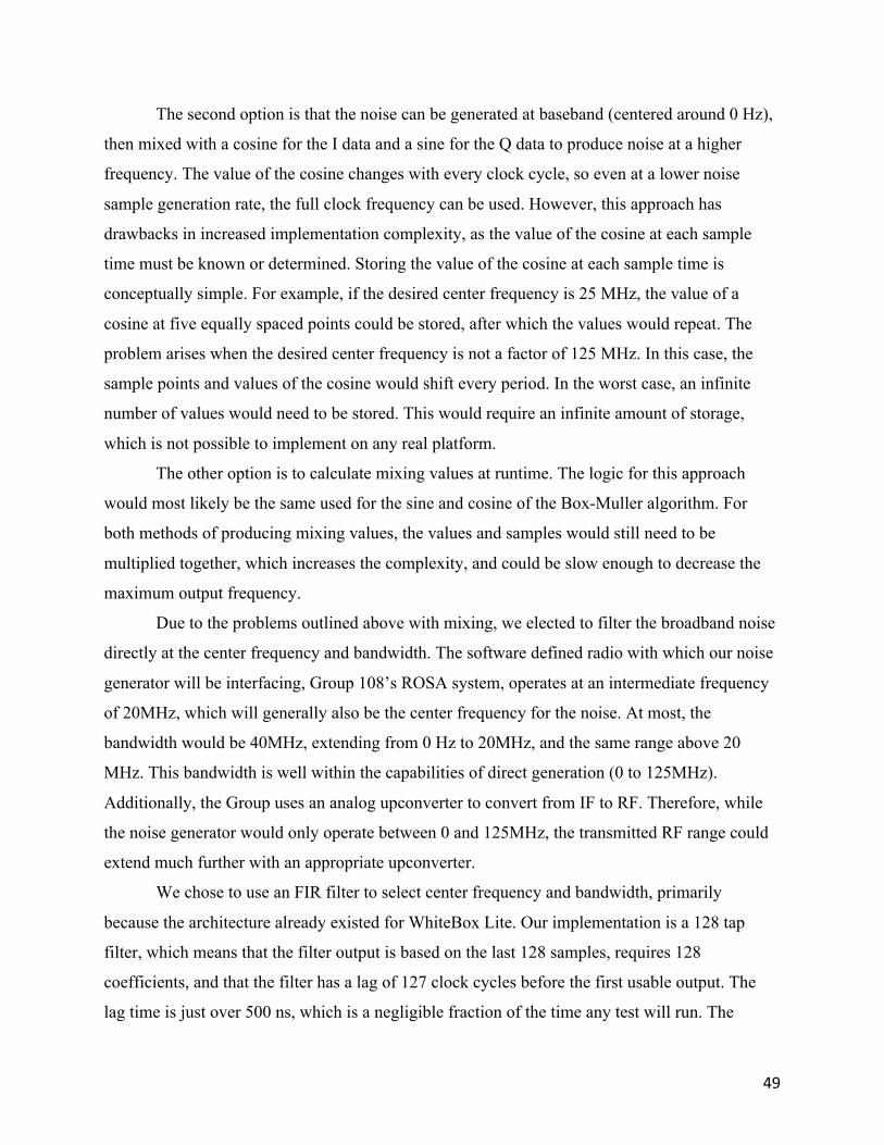
49
The second option is that the noise can be generated at baseband (centered around 0 Hz),
then mixed with a cosine for the I data and a sine for the Q data to produce noise at a higher
frequency. The value of the cosine changes with every clock cycle, so even at a lower noise
sample generation rate, the full clock frequency can be used. However, this approach has
drawbacks in increased implementation complexity, as the value of the cosine at each sample
time must be known or determined. Storing the value of the cosine at each sample time is
conceptually simple. For example, if the desired center frequency is 25 MHz, the value of a
cosine at five equally spaced points could be stored, after which the values would repeat. The
problem arises when the desired center frequency is not a factor of 125 MHz. In this case, the
sample points and values of the cosine would shift every period. In the worst case, an infinite
number of values would need to be stored. This would require an infinite amount of storage,
which is not possible to implement on any real platform.
The other option is to calculate mixing values at runtime. The logic for this approach
would most likely be the same used for the sine and cosine of the Box-Muller algorithm. For
both methods of producing mixing values, the values and samples would still need to be
multiplied together, which increases the complexity, and could be slow enough to decrease the
maximum output frequency.
Due to the problems outlined above with mixing, we elected to filter the broadband noise
directly at the center frequency and bandwidth. The software defined radio with which our noise
generator will be interfacing, Group 108’s ROSA system, operates at an intermediate frequency
of 20MHz, which will generally also be the center frequency for the noise. At most, the
bandwidth would be 40MHz, extending from 0 Hz to 20MHz, and the same range above 20
MHz. This bandwidth is well within the capabilities of direct generation (0 to 125MHz).
Additionally, the Group uses an analog upconverter to convert from IF to RF. Therefore, while
the noise generator would only operate between 0 and 125MHz, the transmitted RF range could
extend much further with an appropriate upconverter.
We chose to use an FIR filter to select center frequency and bandwidth, primarily
because the architecture already existed for WhiteBox Lite. Our implementation is a 128 tap
filter, which means that the filter output is based on the last 128 samples, requires 128
coefficients, and that the filter has a lag of 127 clock cycles before the first usable output. The
lag time is just over 500 ns, which is a negligible fraction of the time any test will run. The
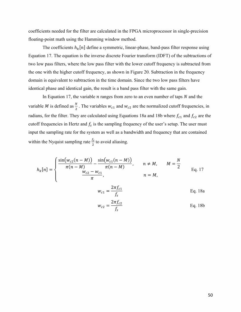
50
coefficients needed for the filter are calculated in the FPGA microprocessor in single-precision
floating-point math using the Hamming window method.
The coefficients ℎX 𝑛 define a symmetric, linear-phase, band-pass filter response using
Equation 17. The equation is the inverse discrete Fourier transform (IDFT) of the subtractions of
two low pass filters, where the low pass filter with the lower cutoff frequency is subtracted from
the one with the higher cutoff frequency, as shown in Figure 20. Subtraction in the frequency
domain is equivalent to subtraction in the time domain. Since the two low pass filters have
identical phase and identical gain, the result is a band pass filter with the same gain.
In Equation 17, the variable 𝑛 ranges from zero to an even number of taps 𝑁 and the
variable 𝑀 is defined as �4 . The variables 𝑤�Z and 𝑤�4 are the normalized cutoff frequencies, in
radians, for the filter. They are calculated using Equations 18a and 18b where 𝑓�Z and 𝑓�4 are the
cutoff frequencies in Hertz and 𝑓6 is the sampling frequency of the user’s setup. The user must
input the sampling rate for the system as well as a bandwidth and frequency that are contained
within the Nyquist sampling rate ��4
to avoid aliasing.
ℎX 𝑛 =
sin 𝑤�4 𝑛 − 𝑀𝜋 𝑛 −𝑀 −
sin 𝑤�Z 𝑛 − 𝑀𝜋 𝑛 −𝑀 , 𝑛 ≠ 𝑀, 𝑀 =
𝑁2
𝑤�4 − 𝑤�Z
𝜋 , 𝑛 = 𝑀,
Eq. 17
𝑤�Z =2𝜋𝑓�Z𝑓6
Eq. 18a
𝑤�4 =2𝜋𝑓�4𝑓6
Eq. 18b
51
Figure 20: Calculating an FIR Band pass Filter Response
The coefficients are calculated on a soft processor using single-precision floating-point
operations and are then stored in registers. On the FPGA, the coefficients pulled from registers,
and within the FIR module, each sample is multiplied by the appropriate coefficients at each
sample time. All the multiplication results are summed to produce the filter output.
User Interface The main method for users to enter their desired amplitude, center frequency and
bandwidth is through a command line interface produced using embedded C code on a soft
processor. We took the command line interface created for WhiteBox Lite and modified it to

52
accept commands specific to our project. The command line interface uses a soft processor to
print byte streams to a terminal window over a serial UART-to-USB connection. The user may
input commands from a set list, which are then sent back to the processor. The set list can be
accessed by typing ‘?’ into the command line. The processor interprets the input and writes data
to custom registers. We added four commands that a user may input to the processor: noise_amp,
set_params, output_sel, and output_mode. We also utilized the existing command ipconfig.
The command noise_amp adjusts the amplitude of the output signal. The command is
performed by typing noise_amp followed by an integer ranging from 0 to 100 that represents a
percentage of the maximum amplitude. The processor converts the integer to a 16-bit fixed-point
number, then writes the result to a register that can be accessed by the FPGA. On the FPGA, the
random numbers that will be fed to the DAC are multiplied by this value using a fixed-point
multiplication module provided by Xilinx. Percentage is represented using 16 unsigned bits.
The command set_params allows a user to select a desired center frequency and
bandwidth. Processing the set_params command is significantly more complicated than
processing noise_amp. The three inputs for the command are integers representing the
bandwidth, center frequency, and sample frequency, all measured in kilohertz (kHz). Since the
number of required coefficients is the number of filter taps plus one, the processor produces 128
coefficients from the given information, which are then stored in registers. The coefficients
define the filter response of an FIR filter implemented in logic on the FPGA.
The processor generates the coefficients using Equations 17, 18a, and 18b. The processor
stores the coefficients in an array and keeps track of the largest and smallest values. These
coefficients are used to determine a constant scaling factor that will be used to scale the
coefficients to 18-bit integers. Without scaling, the coefficients are smaller than 1; thus they
cannot be represented as integers on the FPGA. The scaling factor is computed using Equation
19 and allows the coefficients to be represented over the maximum range of signed 18-bit
number representation. We used 18 bits to represent the coefficients to take full advantage of the
18x18 multipliers on the FPGA. After scaling, the Hamming window function is applied to the
coefficients.
𝑆𝑐𝑎𝑙𝑒 = min 𝑎𝑏𝑠−2Z�
min ℎX 𝑛, 𝑎𝑏𝑠
2Z� − 1max ℎX 𝑛
Eq. 19
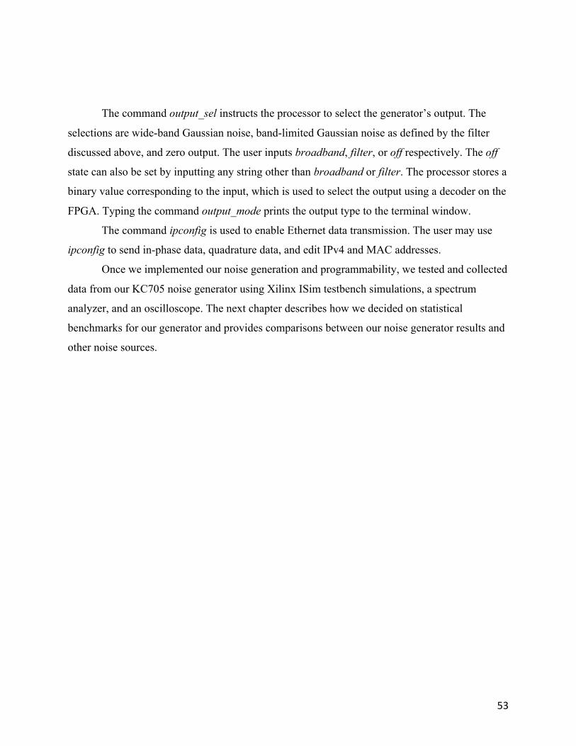
53
The command output_sel instructs the processor to select the generator’s output. The
selections are wide-band Gaussian noise, band-limited Gaussian noise as defined by the filter
discussed above, and zero output. The user inputs broadband, filter, or off respectively. The off
state can also be set by inputting any string other than broadband or filter. The processor stores a
binary value corresponding to the input, which is used to select the output using a decoder on the
FPGA. Typing the command output_mode prints the output type to the terminal window.
The command ipconfig is used to enable Ethernet data transmission. The user may use
ipconfig to send in-phase data, quadrature data, and edit IPv4 and MAC addresses.
Once we implemented our noise generation and programmability, we tested and collected
data from our KC705 noise generator using Xilinx ISim testbench simulations, a spectrum
analyzer, and an oscilloscope. The next chapter describes how we decided on statistical
benchmarks for our generator and provides comparisons between our noise generator results and
other noise sources.

54
4.0 Results This section details the results obtained from tests throughout the project. Section 4.1
covers the results from off-line simulations of software-generated and hardware-generated
random noise. Section 4.2 contains results from testing our FPGA-based noise generator using a
spectrum analyzer and sampling oscilloscope. Section 4.3 addresses the results of tests conducted
using Group 108’s radar test and development system. Throughout the chapter, all statistical tests
were conducted using five runs of 100,000 samples each, and all numerical results presented are
the average values from all five tests. Spectrum plots produced off-line were generated using
MATLAB’s pwelch function on 100,000 samples. Histograms were created (for both off-line
and sampled on-line data) using MATAB’s histfit function and use a standard 100,000 samples
with a bin size of 317, which is the square root of the sample size rounded up to the next integer.
In each histogram, the blue bars show the number of actual samples in each bin. The red line
follows an ideal Gaussian distribution. The full FPGA-based noise generator is shown in Figure
21.
Figure 21: FPGA-based digital noise generator
4.1 Simulation Results The first set of tests conducted was through simulation. Our first test involved a set of
random, normally distributed data produced by MATLAB using the randn function. This

55
function uses a 32-bit Ziggurat algorithm with a period of 264 to produce pseudorandom,
normally-distributed numbers. Uniform numbers for the algorithm are created using shift
registers, but the actual implementation is proprietary. Although MATLAB’s randn function is
not a direct comparison to our hardware Gaussian number generator, we used the data to set a
baseline for what we could expect visually and statistically from a general pseudorandom
number generator. Figure 22 and Figure 23 plot the power spectra and time domain distributions,
respectively, of the MATLAB simulated data.
Figure 22: Power Spectrum of MATLAB Simulated Data
The power spectrum plot frequency axis ranges from 0 to 125 MHz to match that of the
digital noise generator built in this project. To match the DAC output speed on the actual noise
generator, a sampling rate of 250 MHz was assumed.
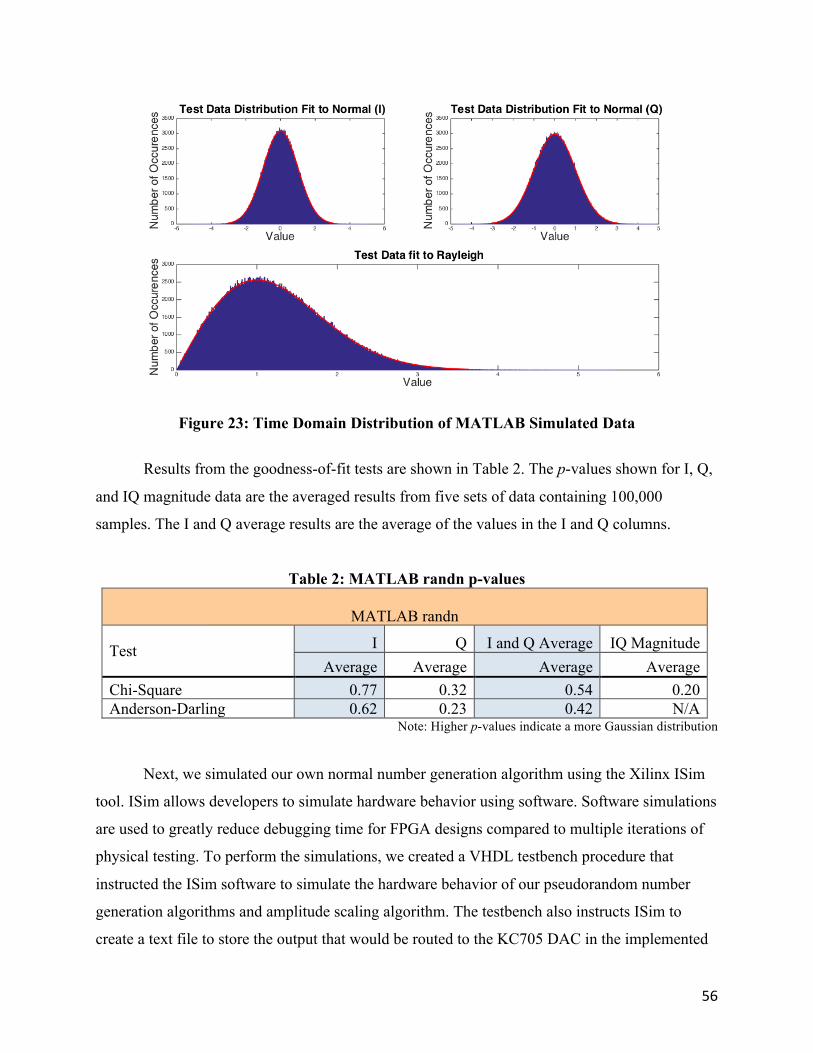
56
Figure 23: Time Domain Distribution of MATLAB Simulated Data
Results from the goodness-of-fit tests are shown in Table 2. The p-values shown for I, Q,
and IQ magnitude data are the averaged results from five sets of data containing 100,000
samples. The I and Q average results are the average of the values in the I and Q columns.
Table 2: MATLAB randn p-values
MATLAB randn
Test I Q I and Q Average IQ Magnitude Average Average Average Average
Chi-Square 0.77 0.32 0.54 0.20 Anderson-Darling 0.62 0.23 0.42 N/A
Note: Higher p-values indicate a more Gaussian distribution
Next, we simulated our own normal number generation algorithm using the Xilinx ISim
tool. ISim allows developers to simulate hardware behavior using software. Software simulations
are used to greatly reduce debugging time for FPGA designs compared to multiple iterations of
physical testing. To perform the simulations, we created a VHDL testbench procedure that
instructed the ISim software to simulate the hardware behavior of our pseudorandom number
generation algorithms and amplitude scaling algorithm. The testbench also instructs ISim to
create a text file to store the output that would be routed to the KC705 DAC in the implemented

57
design. The initial simulation run was our fixed-point Box-Muller algorithm implementation.
The power spectrum in Figure 24 is visually flat and the histograms in Figure 25 clearly shows a
time domain distribution that does not meet our needs. The histograms show too many values
near zero, and too few values at certain points farther out in the tails. Additionally, the statistical
results were all approaching zero, which is not sufficient to pass our tests. Results from the
goodness-of-fit tests are shown in Table 3.
Figure 24: Power Spectrum of Fixed-Point Box-Muller Hardware Simulation
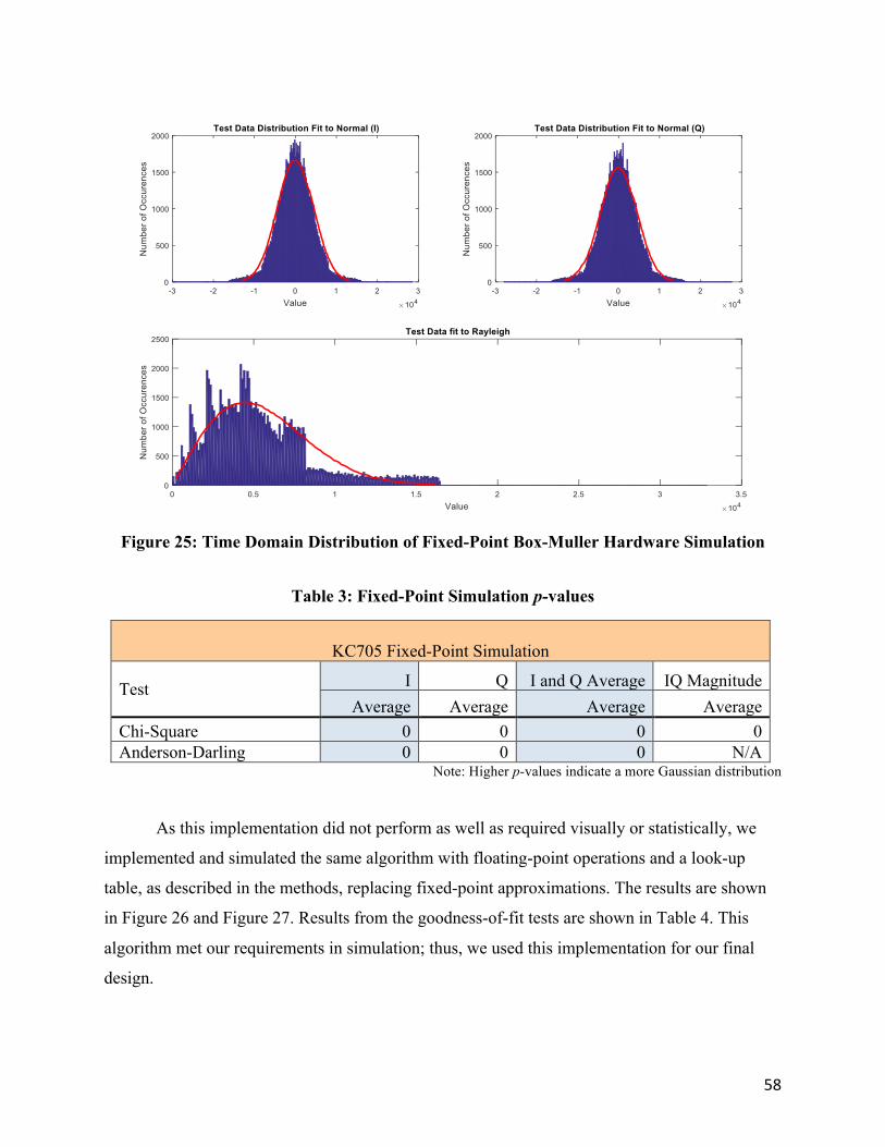
58
Figure 25: Time Domain Distribution of Fixed-Point Box-Muller Hardware Simulation
Table 3: Fixed-Point Simulation p-values
KC705 Fixed-Point Simulation
Test I Q I and Q Average IQ Magnitude Average Average Average Average
Chi-Square 0 0 0 0 Anderson-Darling 0 0 0 N/A
Note: Higher p-values indicate a more Gaussian distribution
As this implementation did not perform as well as required visually or statistically, we
implemented and simulated the same algorithm with floating-point operations and a look-up
table, as described in the methods, replacing fixed-point approximations. The results are shown
in Figure 26 and Figure 27. Results from the goodness-of-fit tests are shown in Table 4. This
algorithm met our requirements in simulation; thus, we used this implementation for our final
design.

59
Figure 26: Power Spectrum of Floating-Point Box-Muller Hardware Simulation
Figure 27: Time Domain Distribution of Floating-Point Box-Muller Hardware Simulation
Table 4: Floating-Point Simulation p-values
KC705 Floating-Point Simulation
Test I Q IQ Average IQ Magnitude Average Average Average Average
Chi-Square 0.31 0.57 0.44 0.55 Anderson-Darling 0.37 0.37 0.37 N/A
Note: Higher p-values indicate a more Gaussian distribution

60
4.2 Output Test Results Once we achieved acceptable simulation results we tested the analog output signal from
the KC705, using both a spectrum analyzer and an oscilloscope. We used a Keysight N9030A
spectrum analyzer to visually inspect the whiteness of the noise. This spectrum analyzer can
measure frequencies from 3 Hz to 2.6 GHz, so we could measure the entire spectrum of our
noise with no risk of aliasing. First, the spectrum of the broadband noise was visually inspected
to ensure that it was an approximately flat line across the generator’s entire frequency range.
While the spectrum is flat up to 80 MHz as shown in Figure 28, it steadily decreases from this
point to the full frequency of 125 MHz. Based on this result, we conducted further testing to
determine the source of the problem. We used a signal generator to produce sine waves at
various frequencies and used the spectrum analyzer to examine their spectra. The spectra were
not attenuated at higher frequencies, which indicated that the measured frequency decline was
occurring in the noise generator hardware.
We collected corresponding time domain data for the noise distribution using a Teledyne
LeCroy SDA 18000 oscilloscope with a bandwidth of 6 GHz and a sampling rate of 20 Gs/s. Due
to limitations of the oscilloscope, the I and Q data were recorded separately at different times and
then combined in MATLAB to conduct our analysis. Since the I and Q outputs of the generator
are statistically independent, combining the data should not affect the analysis of the IQ
magnitude. The broadband noise distribution results in Figure 29 show that the noise is relatively
Gaussian visually; however, the noise does not pass either the chi-square or Anderson-Darling
test. These statistical results are in Table 5.
Figure 28: KC705 Broadband Noise Power Spectrum
KC705 Broadband Power Spectrum
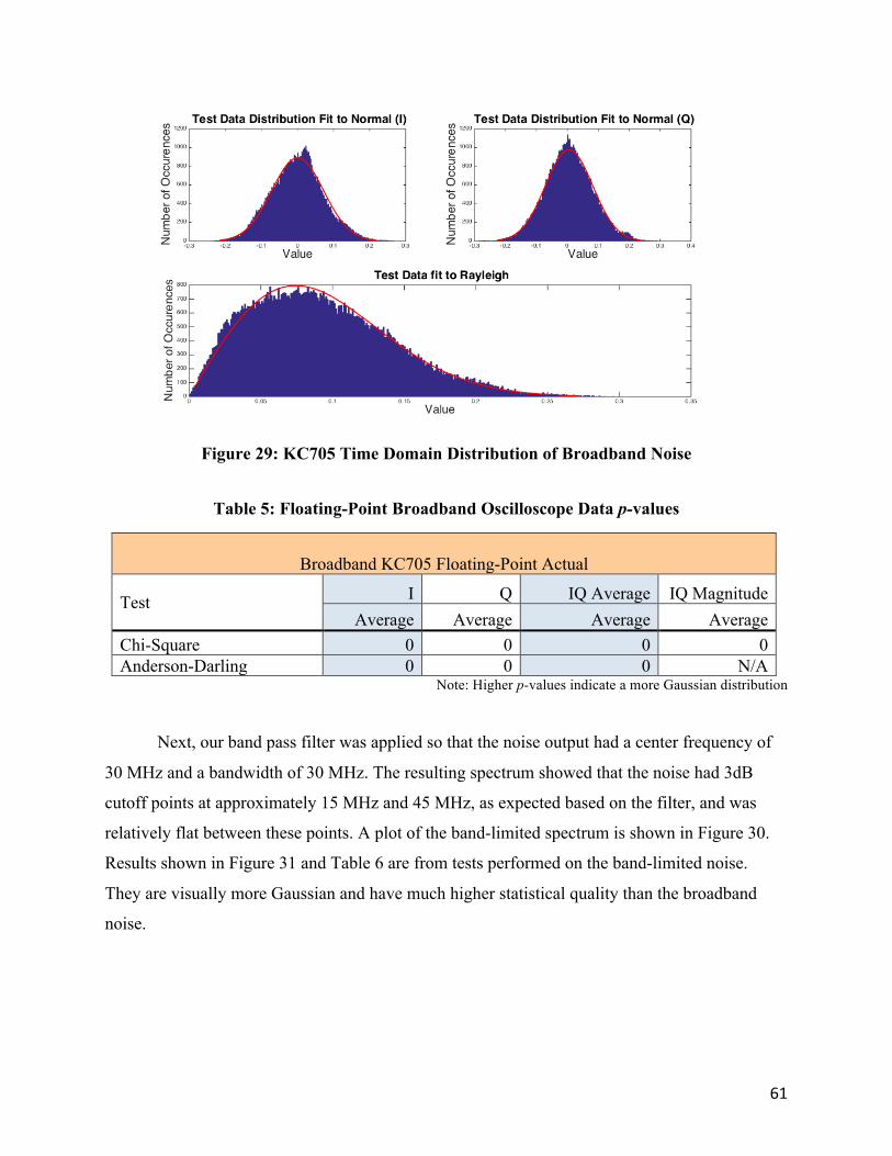
61
Figure 29: KC705 Time Domain Distribution of Broadband Noise
Table 5: Floating-Point Broadband Oscilloscope Data p-values
Broadband KC705 Floating-Point Actual
Test I Q IQ Average IQ Magnitude Average Average Average Average
Chi-Square 0 0 0 0 Anderson-Darling 0 0 0 N/A
Note: Higher p-values indicate a more Gaussian distribution
Next, our band pass filter was applied so that the noise output had a center frequency of
30 MHz and a bandwidth of 30 MHz. The resulting spectrum showed that the noise had 3dB
cutoff points at approximately 15 MHz and 45 MHz, as expected based on the filter, and was
relatively flat between these points. A plot of the band-limited spectrum is shown in Figure 30.
Results shown in Figure 31 and Table 6 are from tests performed on the band-limited noise.
They are visually more Gaussian and have much higher statistical quality than the broadband
noise.
62
Figure 30: Power Spectrum of Band-limited Noise with Bandwidth and Center Frequency
of 30 MHz (3 dB cutoffs marked)
Figure 31: Time Domain Distribution of Band-limited Noise
Table 6: Floating-Point Band-Limited Oscilloscope Data p-values
Band-Limited KC705 Floating-Point Actual
Test I Q IQ Average IQ Magnitude Average Average Average Average
Chi-Square 0.13 0.12 0.12 0.34 Anderson-Darling 0.02 0.03 0.02 N/A
Note: Higher p-values indicate a more Gaussian distribution
KC705 Band-Limited Power Spectrum
63
We also tested WhiteBox Lite’s noise generation method using the same instruments. By
visual inspection of the spectrum and histograms shown in Figure 32 and Figure 33, the noise
produced by the frequency sweep is clearly neither white nor Gaussian. This noise also fails all
of our goodness-of-fit tests as shown in Table 7.
.
Figure 32: Power Spectrum of WhiteBox Lite Frequency Sweep
Figure 33: Time Domain Distribution of WhiteBox Lite Frequency Sweep
64
Table 7: WhiteBox Lite p-values
WhiteBox Lite
Test I Q IQ Average IQ Magnitude Average Average Average Average
Chi-Square 0 0 0 0 Anderson-Darling 0 0 0 N/A
Note: Higher p-values indicate a more Gaussian distribution
4.3 ROSA Data During the early phase of our testing, we used Group 108’s ROSA system to test the
analog noise generator and WhiteBox Lite frequency sweep that we used as benchmarks. We
also tested our fixed-point noise generation algorithm before we decided to improve our
statistical quality by moving to a floating-point algorithm. However, we later discovered that the
processing performed by the ROSA system, which includes mixing, filtering and downsampling
as described in Section 2.3, will make almost any random signal at the input look more Gaussian
at the output. A simulation of the effects of the processing chain on random uniform noise is
shown in Appendix B.
The results of these tests are presented here, but must be evaluated carefully as they do
not accurately reflect the input to the system. Figure 34 is the time domain distribution of the
fixed-point Box-Muller implementation data collected using ROSA and Figure 35 is the time-
domain distribution of WhiteBox Lite’s frequency sweep collected using ROSA. The results are
clearly much more Gaussian than the simulation data shown in Figure 27 and Figure 33.
However, as these results are more Gaussian than unprocessed results would be, we believe they
are useful as an upper limit on how well we could expect our analog noise to perform on any
tests.
65
Figure 34: Time Domain Distribution ROSA Data from Fixed-Point Box-Muller
Figure 35: Time Domain Distribution ROSA Data from WhiteBox Lite
66
5.0 Discussion
After testing our digital noise generator, the team evaluated its strengths and weaknesses.
The generator we developed meets our requirements of programmable amplitude, center
frequency, and bandwidth while displaying strong white and Gaussian characteristics.
Our results show that the power spectrum of our simulated data from Xilinx is flat over
the full 0 to 125 MHz range; however, when producing analog, unfiltered, broadband noise, the
spectrum analyzer showed a relatively flat spectrum from 0 to only approximately 80 MHz.
Starting around 80 MHz, the spectrum analyzer displayed a significant decline in power. This
decline continued to 200 MHz, at which point the analyzer detected no power. To determine
whether the spectrum analyzer or the noise generator was the cause of the power decline at
higher frequencies, we used a Keysight E-series PSG analog signal generator in conjunction with
the spectrum analyzer. We created sinusoidal pulses ranging from 10 MHz up to 200 MHz and
visually inspected the spectrum analyzer for power attenuation at the higher frequency range. We
did not see any attenuation, implying that the power decline is the product of our noise generator.
We identified two possible causes for the power decline at high frequencies. First, the
DAC has a settling time, which is the time interval from when it begins changing voltages to
when it reaches the final voltage. In high frequency applications, the DAC may not be able to
change voltage levels quickly enough, causing a false representation of the input. Since higher
frequencies generally involve greater changes in voltage, this phenomenon would affect higher
frequencies more and cause them to be represented less often. Therefore, the power would be
reduced at these frequencies [Stranneby, 2001]. Additionally, inherent noise in the hardware
could cause bit errors in the DAC that partially account for the low power detections at
frequencies above 125 MHz. From the power spectrum results, we recommend only using our
noise generator to produce frequencies below 80 MHz.
Despite the spectrum limitations of our generator, the output noise is a significant
improvement in whiteness over noise produced by WhiteBox Lite. WhiteBox Lite produces
noise using a frequency sweep carried by a pulse, which is highly deterministic, and the
spectrum results show a regularly spaced series of peaks at different power levels, with the
highest peak at the carrier frequency.
Our noise generator results also show a compelling improvement in normality over
WhiteBox Lite. Our simulation data produces high p-values on the chi-square and Anderson-
67
Darling goodness-of-fit tests, with results comparable to or better than MATLAB’s randn
function. As expected, the corresponding histograms are decidedly Gaussian. Broadband noise
data collected using an oscilloscope produces much lower p-values, but the corresponding
histograms are still visually quite Gaussian. The lower statistical quality may be caused by the
same factors that caused power decline at high frequencies. Since settling time issues primarily
affect larger voltages, they would cause smaller voltages to be represented disproportionately
more often, which appears to be the case in our histograms. Noise in the hardware would explain
signal detection at frequencies above 125 MHz. Additionally, discussion with lab personnel
revealed that the oscilloscope we used likely has an ADC with a resolution of 8 or 10 bits, which
is much lower than the resolution of our noise generator’s DAC. To highlight this difference, the
16-bit DAC used to produce noise on the KC705 can represent up to 65536 possible values,
while an 8-bit ADC can only represent 256 different values. This difference in resolution affects
how samples are divided into bins for analysis, and thus affects statistical test results.
Band-limited noise data collected using the same oscilloscope showed a significant
increase in statistical quality over our broadband noise. This increase in quality is due to the
central limit theorem. As discussed in Section 2.4.3, the central limit theorem can be realized
using a band pass filter. Filtering our noise increased its Gaussian characteristics, which is
reflected in the higher statistical test results.
Data collected from WhiteBox Lite’s frequency sweep are not visually Gaussian. As
expected, applying the chi-square and Anderson-Darling tests to the data produced p-values
approaching zero.
Our noise generator meets the needs of Group 108 and is a significant improvement over
WhiteBox Lite’s method of producing noise. However, we feel that future work can improve its
capabilities.
In addition to producing analog noise, our noise generator can transmit Ethernet packets
containing I or Q data. The goal was to send Ethernet packets with both I and Q data, but due to
time constraints, we were unable to complete the implementation. Also due to time constraints,
we were unable to verify the data within the packets. To realize digital Ethernet with
simultaneous I and Q data output, additional work must be done to change the Ethernet packet
generator module to accept both 16-bit I data and 16-bit Q data as well as modify the packet
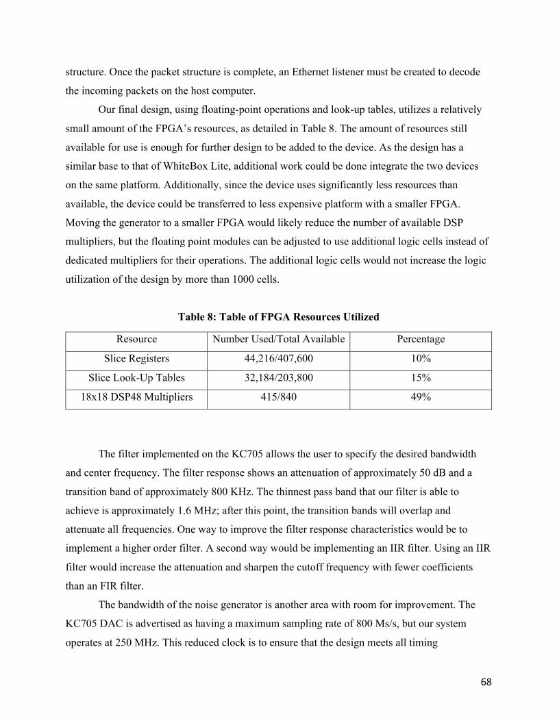
68
structure. Once the packet structure is complete, an Ethernet listener must be created to decode
the incoming packets on the host computer.
Our final design, using floating-point operations and look-up tables, utilizes a relatively
small amount of the FPGA’s resources, as detailed in Table 8. The amount of resources still
available for use is enough for further design to be added to the device. As the design has a
similar base to that of WhiteBox Lite, additional work could be done integrate the two devices
on the same platform. Additionally, since the device uses significantly less resources than
available, the device could be transferred to less expensive platform with a smaller FPGA.
Moving the generator to a smaller FPGA would likely reduce the number of available DSP
multipliers, but the floating point modules can be adjusted to use additional logic cells instead of
dedicated multipliers for their operations. The additional logic cells would not increase the logic
utilization of the design by more than 1000 cells.
Table 8: Table of FPGA Resources Utilized
Resource Number Used/Total Available Percentage
Slice Registers 44,216/407,600 10%
Slice Look-Up Tables 32,184/203,800 15%
18x18 DSP48 Multipliers 415/840 49%
The filter implemented on the KC705 allows the user to specify the desired bandwidth
and center frequency. The filter response shows an attenuation of approximately 50 dB and a
transition band of approximately 800 KHz. The thinnest pass band that our filter is able to
achieve is approximately 1.6 MHz; after this point, the transition bands will overlap and
attenuate all frequencies. One way to improve the filter response characteristics would be to
implement a higher order filter. A second way would be implementing an IIR filter. Using an IIR
filter would increase the attenuation and sharpen the cutoff frequency with fewer coefficients
than an FIR filter.
The bandwidth of the noise generator is another area with room for improvement. The
KC705 DAC is advertised as having a maximum sampling rate of 800 Ms/s, but our system
operates at 250 MHz. This reduced clock is to ensure that the design meets all timing

69
requirements as the same 250 MHz clock is used by almost every module in the system. To
increase the bandwidth of the system, design optimization may allow the DAC sampling rate and
system clock speeds to increase to 350 Ms/s and 350 MHz or higher. Additionally, it may be
useful to determine the frequency response of the DAC. This can be done by generating
sinusoidal signals on the FPGA at varying frequencies up to the Nyquist rate of the DAC.
Viewing the response on a spectrum analyzer would show where the DAC setting time begins to
compromise the output signal.
Another improvement for future work is implementing the noise generator on an Ettus
USRP x310 instead of the KC705. This hardware would improve the generator in three ways.
First, the Ettus comes in an enclosed platform, which is desirable feature over the exposed
hardware of the KC705. Second, the two transmit channels on the Ettus could double the current
bandwidth of the generator. Last, the analog hardware on the Ettus allows for analog mixing.
Mixing using Ettus hardware would allow for a greater range of center frequencies not limited by
the bandwidth of the system, while still maintaining a standalone hardware platform.
It should be noted that the core concept of our design is not limited to FPGAs. The use of
FPGAs was a requirement for our project, but the concept of transforming uniform random
numbers to normally distributed random numbers is applicable to software as well as hardware.
A DAC combined with a microcontroller with enough processing power could produce similar
results, albeit significantly more slowly. Using a larger processor such as a desktop computer is
also possible in the situation where an analog signal is not required or the project is not limited
by size.
70
6.0 Conclusion The goal of this project was to produce a digital Gaussian noise generator with
programmable amplitude, bandwidth, and center frequency. The device had to be a standalone,
FPGA-based hardware platform with the ability to produce noise as an analog signal and in the
form of IQ data in Ethernet packets. We chose to use a Xilinx Kintex-7 DSP development kit
(KC705) as our hardware platform for its wide transmit bandwidth and high FPGA resources.
Additionally, the platform was immediately available for use and Group 108 provided a strong
code base for its development.
We digitally created Gaussian noise by using the Box-Muller transform on uniformly
distributed numbers. The uniform numbers were generated by a Tausworthe algorithm. We used
a soft processor capable of communicating with a host computer to program the noise generator.
A user can select whether to generate broadband noise or band-limited noise, as well as select
output power and center frequency. A user may also choose to transmit I or Q data over Ethernet
instead of transmitting the noise as an analog signal, though the goal of simultaneously
transmitting both I and Q data was not realized. Band-limited noise is produced by passing
broadband noise through a 127th order FIR filter, which has a filter response defined by a user-
selected bandwidth and center frequency.
For testing our noise generator and comparing it to other noise sources, we developed a
set of visual and goodness-of-fit tests. These tests examine the frequency and distribution
characteristics of the noise. We initially analyzed our algorithm using data collected through a
Xilinx testbench simulation, which visually indicated whiteness and normality as well as passing
the goodness-of-fit tests with p-values over 0.4. We then analyzed data from the generator’s
analog output collected using an oscilloscope. The results visually showed white and Gaussian
characteristics, but they were weaker than the simulation. Statistically, the broadband noise
failed the goodness-of-fit tests, while band-limited noise passed the goodness-of-fit tests with p-
values ranging from 0.02 to 0.34.
The digital noise generator presented to Group 108 at the conclusion of this project
produced noise with strong white and Gaussian characteristics and allowed programmable
amplitude, bandwidth, and center frequency. The generator is a standalone, FPGA-based
hardware platform ready for use in a lab environment. With the addition of an up-converter, the

71
device could also be used for field testing. This device will allow the group to further investigate
the effects of noise jamming on various radar systems.

72
Works Cited
Agin, M. A., & Godbole, A. P. (1992). A New Exact Runs Test for Randomness. In C. Page & R. LePage (Eds.), Computing Science and Statistics (pp. 281-285): Springer New York.
Anderson, T. W., & Darling, D. A. (1954). A Test of Goodness of Fit. Journal of the American Statistical Association, 49(268), 765-769. doi:01621459.1954.10501232.
Bird, J. O. (2007). Electrical and Electronic Principles and Technology (3rd ed.). Amsterdam; Boston: Newnes.
Bradley, J. V. (1969). Distribution-Free Statistical Tests. Management Science, 16(1), 141-143. doi:10.2307/2628376.
Callegari, S., Rovatti, R., & Setti, G. (2005). Embeddable ADC-based true random number generator for cryptographic applications exploiting nonlinear signal processing and chaos. IEEE Transactions on Signal Processing, 53(2), 793-805.
Choi, K., Cheun, K., & Jung, T. (2002). Adaptive PN code acquisition using instantaneous power-scaled detection threshold under Rayleigh fading and pulsed Gaussian noise jamming. IEEE Transactions on Communications, 50(8), 1232 - 1235.
Drutarovsky, M., Simka, M., Fischer, V., & Celle, F. (2004). A Simple PLL-Based True Random Number Generator for Embedded Digital Systems. Computing and Informatics, 23, 501–515.
Eaves, J. L., & Reedy, E. K. (1987). Principles of Modern Radar (pp. 265-354, 591-596). New York: Van Nostrand Reinhold.
Gutierrez, R., Torres, V., & Valls, J. (2012). Hardware Architecture of a Gaussian Noise Generator Based on the Inversion Method. Circuits and Systems II, 59(8), 5.
L'Ecuyer, P. (1996). Maximally Equidistributed Combined Tausworthe Generators. Mathematics of Computation, 65, 14.
Lee, D. U., Luk, W., Villasenor, J. D., Guanglie, Z., & Leong, P. H. W. (2005). A hardware Gaussian noise generator using the Wallace method. Very Large Scale Integration (VLSI) Systems, IEEE Transactions on, 13(8), 911-920. doi:10.1109/TVLSI.2005.853615.
Malik, J. S., Malik, J. N., Hemani, A., & Gohar, N. D. (2011). An Efficient Hardware Implementation of High Quality AWGN Generator Using Box-Muller Method. Paper presented at the The 11th International Symposium on Communications & Information Technologies (ISCIT 2011), Hangzhou, China. http://ieeexplore.ieee.org/xpls/abs_all.jsp?arnumber=6090035.
Massa, C. (2015). Personal Communication.
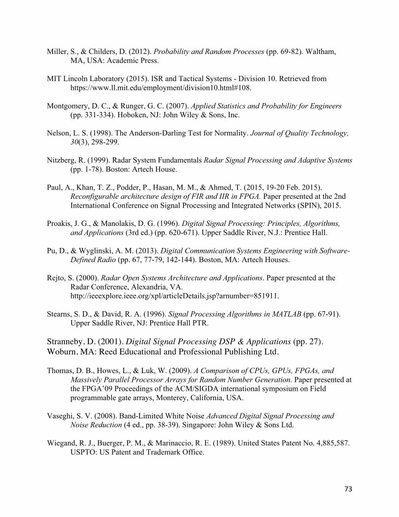
73
Miller, S., & Childers, D. (2012). Probability and Random Processes (pp. 69-82). Waltham, MA, USA: Academic Press.
MIT Lincoln Laboratory (2015). ISR and Tactical Systems - Division 10. Retrieved from https://www.ll.mit.edu/employment/division10.html#108.
Montgomery, D. C., & Runger, G. C. (2007). Applied Statistics and Probability for Engineers (pp. 331-334). Hoboken, NJ: John Wiley & Sons, Inc.
Nelson, L. S. (1998). The Anderson-Darling Test for Normality. Journal of Quality Technology, 30(3), 298-299.
Nitzberg, R. (1999). Radar System Fundamentals Radar Signal Processing and Adaptive Systems (pp. 1-78). Boston: Artech House.
Paul, A., Khan, T. Z., Podder, P., Hasan, M. M., & Ahmed, T. (2015, 19-20 Feb. 2015). Reconfigurable architecture design of FIR and IIR in FPGA. Paper presented at the 2nd International Conference on Signal Processing and Integrated Networks (SPIN), 2015.
Proakis, J. G., & Manolakis, D. G. (1996). Digital Signal Processing: Principles, Algorithms, and Applications (3rd ed.) (pp. 620-671). Upper Saddle River, N.J.: Prentice Hall.
Pu, D., & Wyglinski, A. M. (2013). Digital Communication Systems Engineering with Software-Defined Radio (pp. 67, 77-79, 142-144). Boston, MA: Artech Houses.
Rejto, S. (2000). Radar Open Systems Architecture and Applications. Paper presented at the Radar Conference, Alexandria, VA. http://ieeexplore.ieee.org/xpl/articleDetails.jsp?arnumber=851911.
Stearns, S. D., & David, R. A. (1996). Signal Processing Algorithms in MATLAB (pp. 67-91). Upper Saddle River, NJ: Prentice Hall PTR.
Stranneby, D. (2001). Digital Signal Processing DSP & Applications (pp. 27). Woburn, MA: Reed Educational and Professional Publishing Ltd.
Thomas, D. B., Howes, L., & Luk, W. (2009). A Comparison of CPUs, GPUs, FPGAs, and Massively Parallel Processor Arrays for Random Number Generation. Paper presented at the FPGA’09 Proceedings of the ACM/SIGDA international symposium on Field programmable gate arrays, Monterey, California, USA.
Vaseghi, S. V. (2008). Band-Limited White Noise Advanced Digital Signal Processing and Noise Reduction (4 ed., pp. 38-39). Singapore: John Wiley & Sons Ltd.
Wiegand, R. J., Buerger, P. M., & Marinaccio, R. E. (1989). United States Patent No. 4,885,587. USPTO: US Patent and Trademark Office.

74
Zhang, G., Leong, P. H. W., Lee, D.-U., & Villasenor, J. D. (2005). Ziggurat-based hardware Gaussian random number generator. Paper presented at the International Conference on Field Programmable Logic and Applications.
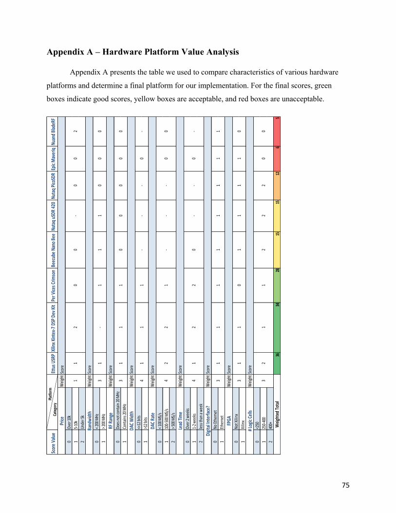
75
Appendix A – Hardware Platform Value Analysis
Appendix A presents the table we used to compare characteristics of various hardware
platforms and determine a final platform for our implementation. For the final scores, green
boxes indicate good scores, yellow boxes are acceptable, and red boxes are unacceptable.
Score V
alue
Ettus USR
PXilinx
Kintex-‐7
DSP D
ev Kit
Per V
ices C
rimson
Beecub
e Nano B
eeNu
taq uS
DR 42
0Nu
taq PicoSD
REpic Maveriq
Nuand B
ladeR
FWeig
htScore
0Ov
er 10
k1
5-‐10k
2Un
der 5k
Weig
htScore
0< 2
00 MHz
1> 2
00 MHz
Weig
htScore
0Do
es no
t con
tain 2
0 MHz
1Co
ntain
s 20 M
HzWeig
htScore
0<=12 bits
1>12 b
itsWeig
htScore
0< 1
00 MS/s
1100-‐5
00 MS/s
2> 5
00 MS/s
Weig
htScore
0Ov
er 2 we
eks
11-‐2
wee
ks2
less than a
wee
kWeig
htScore
0No
Ethe
rnet
1Eth
erne
tWeig
htScore
0No
t Xilin
x1
Xilinx
Weig
htScore
0<250
1250-‐4
002
400+
3634
2815
1512
65
Categ
ory Pla
tform
Price
11
20
0-‐
00
2
Band
width
31
-‐1
11 1
11
1
DAC W
idth
00
0
Digit
al Int
erfac
e?
31
11
1
-‐-‐
00
Lead Time
-‐0
-‐
DAC R
ate
42
21
-‐
41
11
-‐-‐0
00
0
FPGA
-‐0
-‐
RF Ra
nge
31
11
0
41
22
0-‐ 2
20
0
Weig
hted
Total
11
0
# Logic Ce
lls
32
11
2
31
10
11
76
Appendix B – MATLAB Simulation of Uniform Data Through ROSA
Appendix B shows the effects of each stage of the ROSA system’s processing on a
random uniform distribution. For each stage, the left figure shows the time domain distribution
and the right figure shows the frequency domain. These figures indicate that ROSA will make
most distributions look more Gaussian, though the magnitude of this effect will depend on the
original distribution. The MATLAB code used to simulate the data acquisition process on ROSA
is below the following figure.
77
% generate uniform random data in = rand(1,1000000); figure; subplot(4, 2, 1); histogram(in) title('Time Domain Uniform Data into ROSA'); xlabel('Value'); ylabel('Times Occurred'); subplot(4, 2, 2); pwelch(in); title('Frequency Domain Uniform Data into ROSA'); xlabel('Frequency (MHz)'); ylabel('Power'); ylim([-100 0]); % mix with 20 MHz cosine t = ( 0:(length(in)-1) ) / 2e8; mixed = in.*cos(2*pi*2e7*t); subplot(4, 2, 3); histogram(mixed) title('Time Domain Data Mixed by 20 MHz Cosine'); xlabel('Value'); ylabel('Times Occurred'); subplot(4, 2, 4); pwelch(mixed); title('Frequency Domain Data Mixed by 20 MHz Cosine'); xlabel('Frequency (MHz)'); ylabel('Power'); ylim([-100 0]); % Lowpass filter with 5 MHz Cutoff bcoeffs = fir1(128, 5/100, 'low'); filtered = filter(bcoeffs, 1, mixed); subplot(4, 2, 5); histogram(filtered) title('Time Domain Data Lowpass Filtered'); xlabel('Value'); ylabel('Times Occurred'); subplot(4, 2, 6); pwelch(filtered); title('Frequency Domain Data Lowpass Filtered'); xlabel('Frequency (MHz)'); ylabel('Power'); ylim([-100 0]); % downsample by 100 for a 2 MHz acquisition rate downsamp = zeros(1, length(filtered)/100); for i = 1:1:length(filtered)/100

78
downsamp(i) = filtered((i-1)*100 +1); end subplot(4, 2, 7); histogram(downsamp) title('Time Domain Data Lowpass Filtered'); xlabel('Value'); ylabel('Times Occurred'); subplot(4, 2, 8); pwelch(downsamp); title('Frequency Domain Data Lowpass Filtered'); xlabel('Frequency (MHz)'); ylabel('Power'); ylim([-100 0]);