DISCUSSION PAPER SERIES

IZA DP No. 12335

Marcelo BergoloRodrigo CeniGuillermo CrucesMatias GiaccobassoRicardo Perez-Truglia

Tax Audits as Scarecrows. Evidence from a Large-Scale Field Experiment

MAY 2019

Any opinions expressed in this paper are those of the author(s) and not those of IZA. Research published in this series may include views on policy, but IZA takes no institutional policy positions. The IZA research network is committed to the IZA Guiding Principles of Research Integrity.The IZA Institute of Labor Economics is an independent economic research institute that conducts research in labor economics and offers evidence-based policy advice on labor market issues. Supported by the Deutsche Post Foundation, IZA runs the world’s largest network of economists, whose research aims to provide answers to the global labor market challenges of our time. Our key objective is to build bridges between academic research, policymakers and society.IZA Discussion Papers often represent preliminary work and are circulated to encourage discussion. Citation of such a paper should account for its provisional character. A revised version may be available directly from the author.

Schaumburg-Lippe-Straße 5–953113 Bonn, Germany

Phone: +49-228-3894-0Email: publications@iza.org www.iza.org

IZA – Institute of Labor Economics

DISCUSSION PAPER SERIES

ISSN: 2365-9793

IZA DP No. 12335

Tax Audits as Scarecrows. Evidence from a Large-Scale Field Experiment

MAY 2019

Marcelo BergoloIECON-UDELAR and IZA

Rodrigo CeniIECON-UDELAR

Guillermo CrucesCEDLAS-UNLP, University of Nottingham and IZA

Matias GiaccobassoUniversity of California, Los Angeles

Ricardo Perez-TrugliaUniversity of California, Los Angeles

ABSTRACT

IZA DP No. 12335 MAY 2019

Tax Audits as Scarecrows. Evidence from a Large-Scale Field Experiment*

The canonical model of Allingham and Sandmo (1972) predicts that firms evade taxes by

optimally trading off between the costs and benefits of evasion. However, there is no direct

evidence that firms react to audits in this way. We conducted a large-scale field experiment

in collaboration with Uruguay’s tax authority to address this question. We sent letters to

20,440 small- and medium-sized firms that collectively paid more than 200 million dollars

in taxes per year. Our letters provided exogenous yet nondeceptive signals about key inputs

for their evasion decisions, such as audit probabilities and penalty rates. We measured

the effect of these signals on their subsequent perceptions about the auditing process,

based on survey data, as well as on the actual taxes paid, based on administrative data.

We find that providing information about audits had a significant effect on tax compliance

but in a manner that was inconsistent with Allingham and Sandmo (1972). Our findings

are consistent with an alternative model, risk-as-feelings, in which messages about audits

generate fear and induce probability neglect. According to this model, audits may deter tax

evasion in the same way that scarecrows frighten off birds.

JEL Classification: C93, H26, K34, K42, Z13

Keywords: tax, evasion, audits, penalties, frictions

Corresponding author:Ricardo Perez-Truglia405 Hilgard AveLos AngelesCA 90024USA

E-mail: ricardo.truglia@anderson.ucla.edu

* We thank the Uruguay’s national tax administration (Dirección General Impositiva) for their collaboration. We

thank Gustavo Gonzalez for his support, without which this research would not have been possible. We thank

Joel Slemrod for his valuable feedback, as well as that of seminar participants at University of Michigan, University

of California San Diego, Dartmouth University, Universidad Di Tella, Universidad de la Republica, Universidad de

Santiago de Chile, Universidad Católica de Chile, CAF, Banco Central del Uruguay, the 2017 NBER Public Economics

Fall Meeting, the 2017 RIDGE Public Economics Conference, the 2017 Zurich Center for Economic Development

Conference, the 2017 Advances with Field Experiments Conference, the 2018 PacDev Conference, the 2018 AEA

Annual Meetings, the 2018 LAGV Conference, and the 2018 IIPF Annual Congress. This project benefited from

funding by CEF, CEDLAS-UNLP and IDRC.

1 Introduction

Tax audits have been standard tools of most tax administrations throughout history. Auditsincrease tax revenues directly, because firms caught evading must pay taxes on the hiddenincome and corresponding penalties. However, with the exception of large taxpayers, thesedirect revenues are insufficient to make audits cost-effective. Audits play a central role inthe deterrence paradigm of tax evasion: the threat of being audited in the future, of beingcaught evading and having to pay penalties deters firms from evading taxes in the present.

Audits may be useful to foster tax compliance, but there is no direct evidence on howfirms react to audits. The Allingham and Sandmo (1972) model (hereafter, A&S) is thecanonical model of tax evasion in economics. This model is an application of Becker (1968),in which selfish individuals choose whether to engage in criminal activities based on thetradeoff between expected costs and benefits. In A&S, firms choose the optimal amountof income to hide from the tax authority so that the marginal benefits (i.e., the lower taxburden) equal the marginal costs (i.e., the penalties if caught). Whether firms in the realworld react to audits in a calculated manner, as in A&S, is still a source of debate (Almet al., 1992; Dhami and al Nowaihi, 2007; Luttmer and Singhal, 2014; Slemrod, 2018). Inthis study, we provide direct tests of the A&S model based on a high-stakes, large-scale fieldexperiment.

We study a context in which firms should be most attentive to the threat of being audited:small- and medium-sized firms that are subject to the Value Added Tax (VAT). For othersources of taxable income, such as wage income, tax agencies can use third-party reportingto detect evasion automatically. For example, a tax agency can use a computer algorithm tocompare the wage amount reported by an individual and the amount reported by its employerand then automatically notify the individual taxpayers of any discrepancies. Consequently,as individuals earning salaried income are caught evading regardless of whether they areaudited, they should not respond to audits (Kleven et al., 2011). On the contrary, there is nocomparable automatic cross-checking for VAT enforcement.1 Thus, tax authorities must relyheavily on audits to discourage VAT evasion (Gomez-Sabaini and Jimenez, 2012; Bergmanand Nevarez, 2006).

We collaborated with Uruguay’s Internal Revenue Service (from hereon, referred to asIRS) to conduct a natural field experiment with a sample of 20,440 small- and medium-sized firms that are subject to the VAT. For our study, the IRS mailed four different types

1While the VAT requires a paper trail, which is a form of third-party reporting, this paper trail is subjectto significant limitations. Most important, there is no simple algorithm to detect tax evasion automatically.Second, the paper trail breaks down when reaching the consumer (Naritomi, 2016). Third, firms can alsocollude with each other to tamper with the paper trail (Pomeranz, 2015).

2

of letters with information about audits to the owners of each of these firms.2 Some of theinformation contained in each of these letters was randomly assigned, with the goal of testingpredictions of A&S. Using IRS administrative records, we measured the subsequent effects ofthe information contained in the letters on the firms’ compliance with the VAT and other taxresponsibilities in the following year. Additionally, we collaborated with the IRS to conducta post-mailing survey to capture the effect of this information on these firms’ subsequentperceptions about audits.

The first part of the experimental design, following the seminal work by Slemrod et al.(2001), measures how informing taxpayers about tax enforcement affects their tax com-pliance. Firms were randomized into four different letter types: baseline, audit-statistics,audit-endogeneity, and public-goods. The baseline letter type included brief and generic taxinformation that the IRS often includes in its communications with firms. The audit-statisticsletter type was identical to the baseline letter, with additional information about the prob-ability of being audited and the penalty rate, based on tax administration statistics. Therelevant hypothesis is that adding the audit-statistics message to the baseline letter will de-ter tax evasion and thus increase post-treatment tax payments. We also can compare theeffects of this audit-statistics message with the effects of other types of messages. The audit-endogeneity letter provides information about a different feature of the auditing process.The audit-endogeneity letter was identical to the baseline letter, with an additional messageabout how evading taxes increases the probability of being audited. The last letter type wasdesigned to provide a benchmark for a message that might increase tax compliance but doesnot involve the tax audits. The public-goods letter was identical to the baseline letter, with anadditional message describing the social costs from evasion: all the public goods that couldbe provided if tax evasion was lower.

The first part of the results show that, consistent with Slemrod et al. (2001) and thesubsequent literature, informing firms about tax enforcement increases their tax compliance.We find that adding the audit-statistics message to the baseline letter increases tax paymentsby about 6.3%. This effect is economically large: the estimated average VAT evasion rate inUruguay is 26% (Gomez-Sabaini and Jimenez, 2012), meaning that the 6.3% increase equatesto a 24% reduction in VAT evasion. This effect also is highly statistically significant androbust to a number of checks, such as alternative specifications and event-study falsificationtests. The other message related to audits, audit-endogeneity, also significantly increasedtax compliance by about 7.4%. This effect is statistically indistinguishable from the 6.3%effect of the audit-statistics message and robust. In comparison, the public-goods message

2Throughout the paper, for simplicity, we refer to firms’ perceptions and behavior as a shorthand forfirms’ owners or managers perceptions and behavior.

3

had a smaller effect (4.3%) and was statistically insignificant in the baseline specification.Its effect was even smaller in magnitude, and statistically insignificant, in the alternativespecifications.

The main goal of this experiment was not to demonstrate that firms react to informationabout audits but to understand why they react. More precisely, the second and most impor-tant part of the experimental design tests the hypothesis that firms react to information aboutaudits as predicted by A&S. We provide three tests of A&S. The first test exploits surveydata on perceptions about audits. If the audit-statistics letter increased average compliance,to be consistent with A&S, it must be true that this message increased the perceived proba-bility of being audited or the perceived penalty rate. To test this hypothesis, we designed asurvey, to be sent months after the firms received the audit-statistics and audit-endogeneityletters, which measures perceptions about the probability of being audited and the penaltyrate.

The second test of A&S is based on heterogeneity in the signals provided in the letters.We included exogenous, non-deceptive variation in the information about audit probabilitiesand penalty rates in the audit-statistics letter. To generate this information, we computedthe average probabilities and penalty rates using a series of random samples of 50 firms.This sample size was small enough to introduce non-trivial sampling variation in the averageprobabilities and fines shown to the subjects. That is, a given firm could receive a lettersaying that the audit probability is 8%, 10%, or 15%, depending on the sample of similarfirms chosen for that particular letter. These random variations in probabilities and penaltiesshown to the firms allow us to test whether, as predicted by A&S, firms evade less when theyface higher audit probabilities and higher penalty rates.

As a complement to the audit-statistics treatment arm, we designed a separate treatmentarm that created exogenous variation in expected audit probabilities in a more direct way.The audit-threat letter type was sent to a separate sample of firms that was pre-selected bythe IRS for auditing. We randomly divided this set of firms into two groups, one with a 25%probability of being audited and the other with a 50% probability. The audit-threat letterinformed firms of their audit probability. Again, we can test whether, as predicted by A&S,firms evade less when they face a higher audit probability.

The third test of A&S exploits heterogeneity by prior beliefs. According to A&S, thecompliance effect of a given signal about audit probability should depend on the firm’s priorbelief about that probability. For example, a firm receiving a signal that the audit probabilityis higher than its prior belief should increase its tax compliance, while a firm receiving a signallower than its prior belief should decrease its tax compliance. To test this hypothesis, weconstruct a proxy for prior beliefs about audit probability based on variation in the firms’

4

pre-treatment exposure to audits.3

The second part of the results suggests that the effects of the audit-statistics letter are notconsistent with A&S. The results for the first test, based on the survey data, indicate thatthe audit-statistics message reduced the perceived probability of being audited. Accordingto A&S, a reduction in the perceived probability of being audited should have reduced taxcompliance. On the contrary, we find that the audit-statistics message increased averagecompliance.

The second test shows that, contrary to the A&S prediction, the effect of the audit-statistics message does change with the signals of audit probability and penalty rates includedin the letter. The estimated elasticity of tax compliance, with respect to audit probabilitiesand penalty rates, is close to zero and precisely estimated. We find qualitatively and quantita-tively similar effects between the audit-statistics and audit-threat treatment arms. Moreover,we compare our experimental estimates to the results from calibrations of A&S. We reject thenull hypothesis of A&S, even under conservative assumptions about how much firms learnedfrom the audit-statistics message.

The third test also suggests probability neglect (i.e., that our messages had the samepositive effect on tax compliance, regardless of the audit probability communicated in themessage or the firm’s prior belief about such probability). Contrary to the prediction of A&S,the effect of the audit-statistics message did not vary with the firm’s prior belief about theprobability of being audited.

Our findings suggest that small and medium firms may comply with taxes because ofthe threat of being audited but not necessarily in an optimal manner, as predicted by A&S.This leaves open the question of which alternative model best explains the firms’ reactions toaudits. Models of salience (Chetty et al., 2009) and prospect theory (Kahneman and Tversky,1979) explain some but not all findings, such as probability neglect. Instead, our preferredinterpretation is based on the model of risk-as-feelings (Loewenstein et al., 2001).

The models used for choice under risk are typically cognitive; that is, people make de-cisions using some type of expectation-based calculus. The risk-as-feelings model proposesthat responses to fearsome situations may differ substantially from cognitive evaluations ofthe same risks. When fear is involved, the responses to risks are quick, automatic, and intu-itive and thus neglect the underlying probabilities (Sunstein, 2003; Zeckhauser and Sunstein,2010). This risk-as-feelings model can explain our finding of probability neglect. Indeed,

3Take for instance two firms that have been paying taxes for 10 years and, by chance, one of those firmswas audited in the past while the other was not. As a result, the firm that was audited in the past will havea higher belief about the probability of being audited in the future. The implicit assumption is that, dueto the scant information on the auditing process, firms may be forming beliefs about the audit probabilitiesbased on their own exposure to audits.

5

we discuss suggestive evidence that fear plays a significant role in tax compliance. We alsodiscuss policies used by tax agencies around the world that suggest a working knowledge ofthe risk-as-feelings model.

Our study relates to various strands of literature. First, it belongs to a recent but growingliterature that uses field experiments in partnership with tax authorities to study the decisionsof individuals to pay taxes. In a seminal contribution, Slemrod et al. (2001) showed that, for asample of U.S. self-employed individuals, those who were randomly assigned to receive a letterfrom the Minnesota Department of Revenue with an enforcement message reported higherincome in their tax returns. Similar messages about tax enforcement have been shown to havepositive effects on tax compliance in other contexts (for recent reviews, see Pomeranz andVila-Belda, 2018; Slemrod, 2018; Alm, 2019).4 One standard interpretation in this literatureis that taxpayers react to the information about tax enforcement tools and, in line with A&S,reduce their evasion to re-optimize their behavior. However, there is no direct evidence infavor or against this interpretation. Our contribution is to fill this gap in the literature.

This paper is closely related to a group of studies testing the predictions of A&S in alaboratory setting. For example, Alm et al. (1992) conducted a laboratory experiment inwhich undergraduate students play a tax evasion game. Subjects can hide income from theexperimenter, but some subjects are randomly selected to be audited and, if caught evading,must pay a penalty. The authors show that tax compliance in the game increases significantlywith audit and penalty rates, but these effects are economically small and smaller than thosepredicted by optimizing behavior in the context of A&S. The laboratory experiment settingof Alm et al. (1992) and similar studies have several advantages, such as full control overthe rules of the game and freedom in the selection of the model parameters. However, theselaboratory experiments have two main limitations. First, the subjects are typically under-graduate students playing the tax game for the first time and with no prior experience payingtaxes in the real world. In contrast, subjects in our field experiment are experienced firmowners who have been registered with the tax agency, and thus paying taxes, for an averageof 15 years. Second, subjects from laboratory experiments typically pay taxes amounting toless than USD 10. In contrast, subjects in our field experiment paid on average USD 11,800per year, which is in the same order of magnitude as the country’s GDP per capita.5 Wecontribute to this literature by showing that A&S does not fare substantially better in anatural context with experienced subjects and high stakes.

4The following are some examples: Slemrod et al. (2001); Kleven et al. (2011); Fellner et al. (2013);Pomeranz (2015); Castro and Scartascini (2015); Dwenger et al. (2016); Perez-Truglia and Troiano (2018).

5More specifically, in the 12 months before our experiment firms in our sample paid an average of USD7,770 in VAT and USD 4,030 in other taxes. In comparison, the GDP per capita in Uruguay was about USD15,000 in 2015.

6

Our findings also contribute to the more general debate about the determinants of taxcompliance. One of the main puzzles in the literature is that evasion rates seem too low,given the low detection probabilities and penalty rates, especially among smaller firms andself-employed individuals (Luttmer and Singhal, 2014). One traditional explanation for thispuzzle is based on tax morale: firms and individuals do not evade taxes because they do notwant to (Luttmer and Singhal, 2014). Our evidence suggests an alternative explanation forthe puzzle: due to the emotional nature of the decision, taxpayers overreact to the threat ofaudits. In other words, audits may scare taxpayers into compliance in the same way thatscarecrows scare birds. Indeed, this interpretation can explain why, despite the low auditprobabilities and penalty rates, taxpayers seem to be significantly concerned about audits:61% of U.S. taxpayers consider “fear of an audit” to have significant influence on their taxcompliance (United States Internal Revenue Service, 2018).6

Finally, our paper is also part of a recent but growing literature on behavioral firms(DellaVigna and Gentzkow, 2017). We document two sources of profit-maximizing frictions.First, the fact that firms have biases in beliefs about audit probabilities suggests the presenceof information frictions. Second, the fact that tax compliance is inelastic with respect to auditprobability and penalty rates suggests the presence of optimization frictions.

The paper is organized as follows. Section 2 discusses the experimental design. Section 3presents the data sources and discusses the implementation of the field experiment. Section4 presents the results on the average effect of the audit-statistics message, and section 5presents the different tests of A&S. Section 6 discusses the interpretation of the findings.The final section concludes.

2 Experimental Design

Our experiment consisted of a mailing campaign from Uruguay’s IRS with multiple treatmentarms and sub-treatments. Rather than comparing firms that received a letter to firms thatdid not, all of our analyses are based on comparisons between firms that received letterswith subtle variations in their content. We can thus minimize the potential effects of simplyreceiving a letter from the tax authority, which might induce compliance on its own as areminder to pay taxes.

The letters consisted of a single sheet of paper with the name of the recipient in theheader, the official letterhead of the IRS, and the scanned signature of the IRS GeneralDirector. These letters were folded, sealed in an envelope with the official letterhead ofthe IRS on the outside, and sent by certified mail, which guarantees direct delivery to the

6See section 6 for more details about this survey.

7

recipient, who must sign upon receipt.

2.1 Baseline Letter

The first type of letter is the baseline letter, a sample of which is provided in AppendixA.1. The baseline letter contained some information about the goals and responsibilities ofthe tax authority, which the IRS routinely includes in its communications with firms. Itexplained that the individual was randomly selected to receive this information, that theletter was for information purposes only, and that there was no need to reply or to provideany documentation to the IRS. The letters in the other treatment arms included the sametext as in the baseline letter, but also included an additional paragraphs, printed in a largertype size and in boldface.

2.2 Audit-Statistics Letter

In the audit-statistics letter type, we added a paragraph to the baseline letter, providingfirms with information about the audit and penalty rates. According to the Allinghamand Sandmo (1972) model, we expect risk-averse firms to be interested in this information,because it helps them optimize their evasion decisions and potentially increase their bottomline.7 Furthermore, this information should be particularly valuable in the context of limitedinformation about audits. For instance, it is easy to find information online about factorspotentially relevant for firms’ decision-making, such as inflation and exchange rates. However,it is extremely difficult to find any information about audit probabilities and actual penaltiespaid by evading firms. Tax authorities seem to prefer to conceal this information.

Appendix A.2 presents a sample of the audit-statistics letter type. The additional para-graph included information about audit probabilities (p) and penalty rates (θ) for a randomsample of firms that were similar to the recipient, as follows:

“On the basis of historical information on similar businesses, there is a probabilityof [p%]that the tax returns you filed for this year will be audited in at least oneof the coming three years. If, pursuant to that auditing, it is determined that taxevasion has occurred, you will be required to pay not only the amount previouslyunpaid, but also a fee of approximately [θ%] of that amount.”

Note that we communicated the probability that firms will be audited in at least one of thethree following years, because IRS experts stated that this was the relevant probability for

7We assume that firms in our sample are risk averse, which is plausible since we deal mainly with smalland medium firms. However, A&S has been generalized to settings with risk-neutral agents (Reinganum andWilde, 1985; Srinivasan, 1973).

8

firms’ decision-making. Uruguay’s tax law indicates that tax audits should cover the previousthree years of tax returns and, as a result, the probability that the current year’s tax reportwill be audited is roughly equal to the probability that the firm will be audited at least onceover the following three years.

In our sample, the average value of p is 11.7%, and the average value of θ is 30.6%.Tax agencies in most countries do not publish data on the values of p and θ, which makesit difficult to compare the Uruguayan case to other contexts. In the United States, forwhich some comparable data are available, these two parameters are on the same order ofmagnitude: self-employed individuals face a p of 11.42% and a base θ of 20%.8

The goal of this treatment arm was to generate exogenous variation in the firms’ percep-tions about audit probabilities and penalty rates. Because of legal and other constraints, wecould not assign different firms to different sets of information about these factors. We insteadinduced non-deceptive, exogenous variation in messages that may affect these perceptions byexploiting the sampling variation in statistics about audits and penalties.

More specifically, we divided the firms into five groups of “similar firms,” correspondingto the five quintiles of total VAT payments in the fiscal year before our intervention. For eachfirm, we then drew a random sample of 50 other firms from the same quintile (i.e., similarfirms), from which we computed the averages of p and θ. This randomization strategy gen-erated 940 different combinations of p and θ. These estimates of p and θ were unbiased andconsistent with the explanation given in a footnote that we included in the letter, thus infor-mation provided to recipients was nondeceptive. The footnote explained how we estimatedthe values of p and θ:

“Estimates are based on data from the 2011–2013 period for a group of firms withsimilar characteristics, for instance, in terms of total revenue. The probabilityof being audited was calculated as a percentage of audited firms in a randomsub-sample of firms. The rate of the fee was estimated as an average of a randomsub-sample of audits.”

The values of p ranged from 2% to 25%, with an average of about 11.7%. The values ofθ ranged from 15% to 68%, with an average of about 30.6%. Figure 1 presents the auditprobability and penalty size distribution across five groups by firm size (one in each row)

8First, there is an annual probability of being audited of 2.1%, according to the ratio of returns examinedfor businesses with no income tax credit and with a reported income between USD 25,000 and 200,000 (Table9a of IRS, 2014). Each audit covers the previous 3 to 6 years, which implies that the the probability thatthe current year’s tax filing will be eventually audited ranges from 5.88% to 11.42%. Second, IRS usuallyimposes a basic penalty of θ=20%, although the penalties can be higher in more severe cases.

9

and the distribution of the generated within-group parameters.9 The vertical line denotesthe average probability based on all members of the group. If we based our estimates of pand θ included in the letter on the population of firms, every member of the group wouldhave received the same signal (the vertical line). As we computed p and θ from samplesof 50 firms, the sampling variation implies that different members of each group receiveddifferent signals. For example, Figure 1.a.1. shows that in group 1, the average p for allgroup members is 8.1%, whereas the histogram depicts the different signals actually sent tofirms within the group. These signals center around the average p, but they range from 2.5%to 20%. Note the differences in the vertical lines across groups: for firms in the first quintile,the average randomized p is 8.1%, and this value increases monotonically up to 13.4% forthose in the top quintile. This means that a small share of the variation across subjects inthe values of p and θ included in the letter results from non-random variation across groups,whereas the within-group variation is fully due to random variation, which is an importantfactor for the following econometric model.10

2.3 Audit-Threat Letter

To complement the evidence from the audit-statistics sub-treatment, we implemented analternative way of randomizing perceptions about audit probabilities using an audit-threatletter. We devised a treatment arm that randomly assigned firms to groups with differentprobabilities of being audited in the following year. A sample of the audit-threat letter ispresented in A.3. The audit-threat letter was identical to the baseline letter, with the followingadditional paragraph:

“We would like to inform you that the business you represent is one of a groupof firms pre-selected for auditing in 2016. A [X%] of the firms in that group willthen be randomly selected for auditing.”

This audit-threat treatment arm was applied to a separate experimental sample, a groupof high-risk firms selected by the IRS audit department. The recipients of the audit-threatletter thus cannot be compared to those of the baseline letter. Instead, we randomly assignedthe firms in this treatment arm to two groups, one with a probability of being audited inthe following year of 25% (X=25%) and another with a probability of being audited twiceas large (X=50%). These messages were non-deceptive: the audit department provided a

9We constructed the 5 groups according to the quintiles of VAT paid during the tax year before ourintervention.

10To measure the share of the variation that corresponds to the cluster size, we regress each parameter onthe quintiles of VAT payments. Regressing p over pre-treatment VAT quintiles dummies results in R2 = 0.118,while regressing θ over the same dummies results in R2 = 0.007.

10

commitment that they would conduct audits according to these probabilities in the followingyear.

2.4 Audit-Endogeneity Letter

The audit-statistics and audit-threat treatment arms conveyed quantitative information aboutaudit probabilities and penalty rates. We also wanted to incorporate into our research design amessage about a different aspect of the audit process. Most tax agencies, including Uruguay’s,account for firm characteristics when deciding which ones to audit. They assign higheraudit probabilities to firms with higher evasion risk. As a result, evading taxes typicallyincreases the probability of being audited. This factor was incorporated as a special case inA&S, in which audit probabilities were determined endogenously. If unsuspecting firms learnabout the endogenous nature of their audit probabilities, they should revise their tax evasiondecisions and reduce the amount of tax evaded.11

We used this insight from economic theory to devise the audit-endogeneity message aboutthe nature of the audit process. We asked our counterparts at the IRS to use their evasion-risk scores to divide a small sample of firms into two groups: those suspected of evading taxesand those not suspected of evading taxes. We then computed the difference in audit ratesfrom 2011–2013 between the two groups: the rates were approximately twice as high for theformer group. We used this information to create the message in the audit-endogeneity lettertype, which was identical to the baseline letter with the addition of the following paragraph(see sample in Appendix A.4):

“The IRS uses data on thousands of taxpayers to detect firms that may be evadingtaxes; most of its audits are aimed at those firms. Evading taxes, then, doublesyour chances of being audited.”

2.5 Public-Goods Letter

We also devised a treatment arm to provide a benchmark for the effect of messages intendedto increase tax compliance without directly mentioning audits. In line with previous studies(see Blumenthal et al., 2001; Fellner et al., 2013; Pomeranz, 2015; Dwenger et al., 2016),we wanted to include a message that would leverage non-pecuniary motives to increase taxcompliance. We designed a non-pecuniary message that was expected to be most effectiveat increasing compliance by the IRS staff and authorities: a message providing information

11Konrad et al. (2016) present suggestive evidence of this mechanism in the context of a laboratory exper-iment: taxpayers facing a situation where suspicious attitudes toward tax officers increase the probability ofbeing audited increase their tax compliance by 80%.

11

about the cost of evasion in terms of the provision of public goods, in the spirit of the modelof Cowell and Gordon (1988).12

The public-goods letter is identical to the baseline letter, with the addition of a specificparagraph listing a series of services that the government could provide if tax evaders reducedtheir evasion by 10% (see Appendix A.5 for a sample of the letter):

“If those who currently evade their tax obligations were to evade 10% less, theadditional revenue collected would enable all of the following: to supply 42,000portable computers to school children; to build 4 high schools, 9 elementaryschools, and 2 technical schools; to acquire 80 patrol cars and to hire 500 policeofficers; to add 87,000 hours of medical attention by doctors at public hospitals;to hire 660 teachers; to build 1,000 public housing units (50m2 per unit). Therewould be resources left over to reduce the tax burden. The tax behavior of eachof us has direct effects on the lives of us all.”

We used estimates from different governmental agencies to make the calculations reflected inthis message.13

2.6 Survey Design

We designed a survey to be conducted with a sample of owners from our main subject pool,months after they received the letters. The IRS, with the support of the Inter-AmericanCenter of Tax Administrations and the United Nations, had previously administered a surveyon the costs of tax compliance for small- and medium-sized businesses. We collaborated withthe tax authority in the design and implementation of a new survey, which included a specificmodule tailored for our research design. The survey also included seven additional modules,designed by the IRS, about the costs of tax compliance and other topics. Appendix A.6 showsa sample of the email with the invitation to participate in the online survey. We partneredwith local and international universities to increase respondent confidence and to highlightthat the survey was part of a scientific study and not an audit or compliance exercise by theIRS.

To further ensure trustworthy responses, the IRS assured potential respondents that thesurvey responses would remain anonymous and that they could not be traced back to specific

12This message is also related to the laboratory experiment from Alm et al. (1992), which presents evidencethat one of the reasons why people decide to pay taxes is their valuation of the public goods provided bymeans of the tax revenues.

13These agencies were: Administracion Nacional de Educacion Publica (ANEP), CEIBAL, Ministerio deSalud Publica (MSP), Ministerio del Interior (MI), Ministerio de Vivienda, Ordenamiento Territorial y MedioAmbiente (MVOTMA).

12

individuals or firms. To measure the effect of our experiment on these survey responses, weembedded a code in the survey link to identify the treatment arm of the experiment to whichthe recipient was assigned. These codes did not uniquely identify any single firm, but theyallowed us to link treatment arms and survey responses while maintaining the anonymity ofresponses.

Appendix A.7 shows a snapshot of our survey module. We designed questions to assesswhether the audit-statistics message shifted perceptions of the recipients of our letters, bymeans of the two following questions:

Perceived Audit Probability: “In your opinion, what is the probability that thetax returns filed by a company like yours will be audited at least in one of thenext three years (from 0% to 100%)?”

Perceived Penalty Rate: “Let us imagine that a company like yours is auditedand that tax evasion is detected. What, in your opinion, is the penalty (in %)as determined by law that the firm must pay in addition to the originally unpaidamount? For example, a fee of X% means that, for each $100 not paid, the firmwould have to pay those original $100 plus $X in penalties.”

After each question, we elicited how certain the subject felt about his or her response on ascale from 1 to 4, where 1 is “not at all sure” and 4 is “very sure.” For the sake of completeness,we also included a question in the survey to measure the subject’s awareness about theendogeneity of audit probabilities. This question and its results are described in detail inAppendix B.3.2.

3 Data Sources and Implementation of the Field Ex-periment

3.1 Institutional Context

Uruguay is a South American country with an annual GDP per capita of about USD 15,000in 2015. Total tax revenues (i.e., for all levels of government) were about 19% of GDP in2015 and, as is common in many countries, VAT represents the largest source of tax revenue,accounting for roughly 50% of the total tax collection.14 Firms are required to remit VAT

14Own calculations based on data from the Central Bank of Uruguay and from the Internal RevenueService. Other sources of tax revenues include the personal income tax, the corporate tax, and some specifictaxes to consumption, businesses and wealth.

13

payments all along the production and distribution chain.15 The standard VAT rate is 22%.16

Our main focus is on the VAT, which represents the largest tax liability for firms inUruguay. An important factor in our context is that VAT has limited third-party reporting.The amounts reported for other sources of taxable income are subject to automatic third-party reporting, and thus taxpayers would be caught evading even without audits. Forinstance, wage income is hard to conceal in modern economies, because employers are usuallyrequired to report their employees’ earnings to the tax authority. Consequently, tax evasioncan be detected and deterred even without conducting an audit (Kleven et al., 2011). Evenif VAT requires a paper trail, this reporting has significant limitations in practice. The papertrail breaks down when reaching the consumer, and firms can collude with each other orwith customers to tamper with the paper trail, for instance, by offering discounts for saleswithout receipts (Pomeranz 2015; Naritomi 2016).17 In this institutional setting and in thecase of VAT liabilities for small and medium firms, audits represent the main tool for evasiondeterrence. They are the primary mechanism through which tax administrations can detectand deter VAT evasion (Gomez-Sabaini and Jimenez, 2012; Bergman and Nevarez, 2006).

Uruguay does not seem an atypical country in terms of tax evasion and tax morale.According to estimates from Gomez-Sabaini and Jimenez (2012), evasion of VAT in Uruguaywas around 26% in 2008. This is the third-lowest rate among the nine Latin Americancountries included in the study and comparable to evasion rates in more developed economies.For example, similar computations suggest an evasion rate of 22% for Italy in 2006 (Gomez-Sabaini and Moran, 2014).18 Regarding tax morale, we used data from the 2010–2013 waveof the World Values Survey. According to this data, 77.2% of respondents from Uruguaystated that evading taxes is “Never Justifiable,” whereas this proportion is 68.2% on average(population-weighted) for all other Latin American countries and 70.9% for the United States.

15Firms may credit VAT paid on input costs (i.e., imports and purchases from their suppliers) against thetotal sales of goods and services to their costumers (i.e., “tax debit”). They pay VAT to the IRS only onthe excess of the total “tax debit” over the tax credit. If the tax credit exceeds the debit, the excess may becarried over for future tax years. While the VAT should in theory be similar in its effects to a retail salestax, in practice the two types of taxes differ in some substantial aspects (Slemrod, 2008).

16A small number of products considered basic necessities either have a 10% rate or are exempt from thetax.

17At the time of our experiment, firms the IRS had not yet implemented standardized electronic receipts.In the future, these electronic systems may facilitate and automatize the cross-check of the VAT trail todetect evasion.

18Gomez-Sabaini and Jimenez (2012) compute those rates by applying the “indirect” method to estimatetax evasion. This method is based on the comparison of collected VAT to aggregate consumption data fromthe System of National Accounts (SNA).

14

3.2 Subject Pool and Randomization

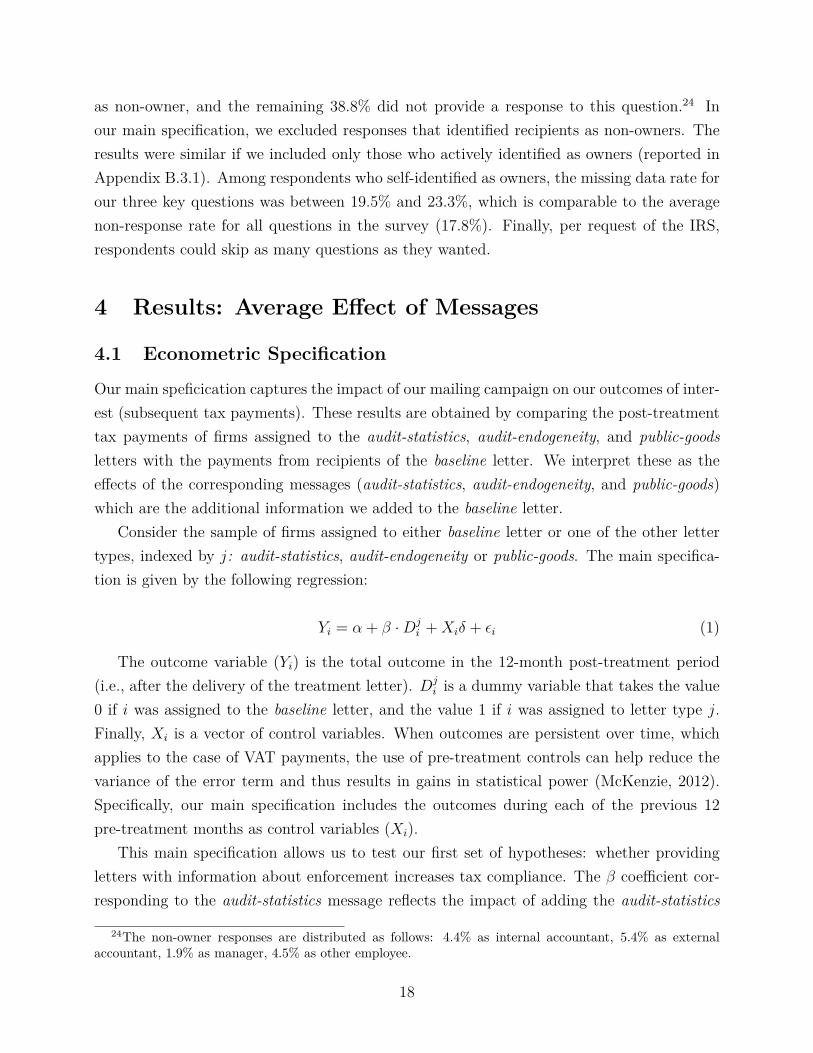
Our experiment was conducted in collaboration with the IRS of Uruguay. As of May 2015,there were 120,142 firms registered in the agency’s database. A subsample of 4,597 firms,preselected by the IRS, was put aside for the audit-threat sample, which we call the secondaryexperimental sample. Of the remaining firms, we followed a series of criteria to select ourmain experimental sample. We first excluded some firms by request of the IRS. For instance,we excluded firms subject to special regimes for VAT payments (very small or very largefirms). We also kept in the experimental sample only those firms that made VAT paymentsin at least three different months in the previous 12-month period and those with a totalvalue of at least USD 1,000.19

To maximize the impact of our information provision experiment, we did our best toensure that the letters would be delivered to the firms’ owners.20 Moreover, in very largefirms, the effect of the information could be substantially diluted, as it may not reach theowner or the individuals making decisions about tax compliance. Thus, we excluded from oursubject pool firms with a total value exceeding USD 100,000 during the previous 12 months.

These criteria left a subject pool of 20,471 firms for the main experimental sample. Allfirms were randomly assigned to receive one of the four letter types, with the followingdistribution: 62.5% were assigned to the main treatment arm (audit-statistics letter), and12.5% were assigned to each of the three remaining letter types (baseline, audit-endogeneity,and public-goods).21 After removing the roughly 18.5% of letters that were returned bythe postal service, the final distribution of letter types was as follows: 10,272 received audit-statistics; 2,064 received baseline; 2,039 received audit-endogeneity; and 2,017 received public-goods letters (total N = 16,392). The 4,597 firms in the secondary sample were assigned toreceive the audit-threat letter. Half were randomly assigned to the message of a 25% auditprobability, and the other half to the 50% audit probability. After excluding the 12% ofletters returned by the postal service, we were left with 2,015 firms in the 25% probabilitygroup and 2,033 firms in the 50% probability group (total N = 4,048). Table 1 provides somedescriptive statistics for the firms in our subject pool. The firm characteristics include VATpayments right before we sent the mailing, the age of the firm, the number of employees, andother basic variables. Column (2) corresponds to all firms in the main experimental sample.

19The sample selection was conducted in May 2015, so this 12-month period spans from April 2014 toMarch 2015.

20In some cases, owners provide the address of external accountants instead of their own or their firms.We removed from the sample firms that were registered with an accountant’s mailing address as their own(the IRS keeps records of addresses for all registered accountants).

21The randomization to letter types was stratified by the quintiles of the distribution of VAT paymentsover the fiscal year before our intervention.

15

On average, firms had 4.8 employees, had been registered with the IRS for 15.3 years, and14% had been audited at least once over the previous three years. For comparison, column(1) of Table 1 shows the same statistics for the universe of all registered firms. By design,firms in our experimental sample are smaller, both in terms of number of employees and inlevel of VAT payments. Finally, column (3) of Table 1 provides statistics about the secondaryexperimental sample (i.e., audit-threat treatment arm). Despite some statistically significantdifferences in the two groups, the firms are broadly comparable in size. The main differencebetween firms in the two experimental samples is that the audit rates were 9 percentage pointshigher in the audit-threat sample. This difference is by design, because the IRS selected firmsclassified as high-risk for this treatment arm, and these firms had a higher propensity to betargeted for audits in the past.

Table 2 allows us to compare the balance of pre-treatment characteristics between firmsassigned to the different letter types. Columns (1) through (4) correspond to firms in themain experimental sample. For each characteristic, column (5) presents the p-value of thetest of the null hypothesis that the averages for these characteristics are the same across allfour letter types. As expected, the differences across letter types are economically small andstatistically insignificant. Columns (6) through (8) of Table 2 present a similar balance test,except for the secondary sample used for the audit-threat arm. Again, the characteristics arebalanced across the two sub-treatments in the audit-threat treatment arm.

3.3 Outcomes of Interest

The letters were provided to Uruguay’s postal service on August 21, 2015. The vast majorityof the letters were delivered during September, and therefore we set August as the last monthof the pre-treatment period and October as the first month of the post-treatment period.The main outcome of interest in our study is the total amount of VAT liabilities remittedby taxpayers in the 12 months after receiving the letter.22 To test for the persistence ofour treatment effects, we defined a second period of observation between October 2016 andSeptember 2017 (i.e., up to two years after the intervention).

On average, the total amount of VAT paid by firms that received the baseline letterin the 12-month pre-treatment period was about USD 7,700, whereas the amount for thecorresponding post-treatment period was approximately USD 6,500. This negative trendin VAT payments can be explained by the fact that this sample contains a high share ofsmall firms with a high turnover rate. The size of post-treatment VAT payments variedsubstantially, ranging from the 10th percentile of USD 400 to the 90th percentile of USD

22This variable includes all VAT payments, including direct VAT payments and indirect VAT withholdings.

16

16,550.23

We can further break down firms’ VAT payments according to their timing. We canobserve the date of transfer to the IRS as well as the month for which the payment wasimputed. Firms can back-date payments to cover liabilities from previous periods. As firmstypically make VAT payments on a monthly basis, they normally cover the current andprevious months, which we call concurrent payments. We classified payments for two ormore months in the past as retroactive payments. About 99.4% of firms made at least oneconcurrent payment in the 12-month pre-treatment period, whereas only 23.8% of firms madeat least one retroactive payment over this same period.

Finally, although we focused on VAT payments in our analysis, we obtained data fromthe IRS on the other main taxes paid by the firms, such as corporate income taxes and networth taxes. These two taxes and the VAT jointly represent more than 96% of the total taxburden of firms. We used payments of these taxes as additional outcomes of interest to studywhether firms effectively changed their overall compliance or if they substituted evasion ofVAT for that of other taxes.

3.4 Survey Implementation

The IRS communicates mainly by postal mail, and it thus has mailing addresses for allregistered firms. It also keeps records of email addresses for a subset of firms that have usedtheir online services. We emailed invitations to all firms in the main experimental samplewith a valid email address. Our intention was to survey firms soon after they received ourletters, but the survey was postponed due to implementation challenges. We sent emailinvitations to participate in the online survey to 3,845 firms in May 2016, about nine monthsafter our mailing experiment. Table 1 shows that the firms we invited to the survey (column(5)) were similar in characteristics to those in the main experimental sample (column (2)).

Our purpose was to elicit the beliefs of firm owners. We did not include email addressesthat were repeated more than three times in the full sample, as these most likely correspondedto accounting firms representing multiple small and medium enterprises. Even after applyingthis criteria, the IRS records could not ensure that the registered email address correspondedto the firms’ owners. We thus asked the survey respondent to self-identify as one of thefollowing five types: owner, internal accountant, external accountant, manager, or otheremployee. From the 3,845 recipients that we invited to participate in the survey, we received2,331 responses (response rate of 60.6%). Of these 2,331, 45% self-identified as owner, 16.2%

23Table B.1 in Appendix B.1 presents detailed descriptive statistics about the distribution of pre- andpost- treatment payments for firms that received the baseline letter type.

17

as non-owner, and the remaining 38.8% did not provide a response to this question.24 Inour main specification, we excluded responses that identified recipients as non-owners. Theresults were similar if we included only those who actively identified as owners (reported inAppendix B.3.1). Among respondents who self-identified as owners, the missing data rate forour three key questions was between 19.5% and 23.3%, which is comparable to the averagenon-response rate for all questions in the survey (17.8%). Finally, per request of the IRS,respondents could skip as many questions as they wanted.

4 Results: Average Effect of Messages

4.1 Econometric Specification

Our main speficication captures the impact of our mailing campaign on our outcomes of inter-est (subsequent tax payments). These results are obtained by comparing the post-treatmenttax payments of firms assigned to the audit-statistics, audit-endogeneity, and public-goodsletters with the payments from recipients of the baseline letter. We interpret these as theeffects of the corresponding messages (audit-statistics, audit-endogeneity, and public-goods)which are the additional information we added to the baseline letter.

Consider the sample of firms assigned to either baseline letter or one of the other lettertypes, indexed by j: audit-statistics, audit-endogeneity or public-goods. The main specifica-tion is given by the following regression:

Yi = α + β ·Dji +Xiδ + εi (1)

The outcome variable (Yi) is the total outcome in the 12-month post-treatment period(i.e., after the delivery of the treatment letter). Dj

i is a dummy variable that takes the value0 if i was assigned to the baseline letter, and the value 1 if i was assigned to letter type j.Finally, Xi is a vector of control variables. When outcomes are persistent over time, whichapplies to the case of VAT payments, the use of pre-treatment controls can help reduce thevariance of the error term and thus results in gains in statistical power (McKenzie, 2012).Specifically, our main specification includes the outcomes during each of the previous 12pre-treatment months as control variables (Xi).

This main specification allows us to test our first set of hypotheses: whether providingletters with information about enforcement increases tax compliance. The β coefficient cor-responding to the audit-statistics message reflects the impact of adding the audit-statistics

24The non-owner responses are distributed as follows: 4.4% as internal accountant, 5.4% as externalaccountant, 1.9% as manager, 4.5% as other employee.

18

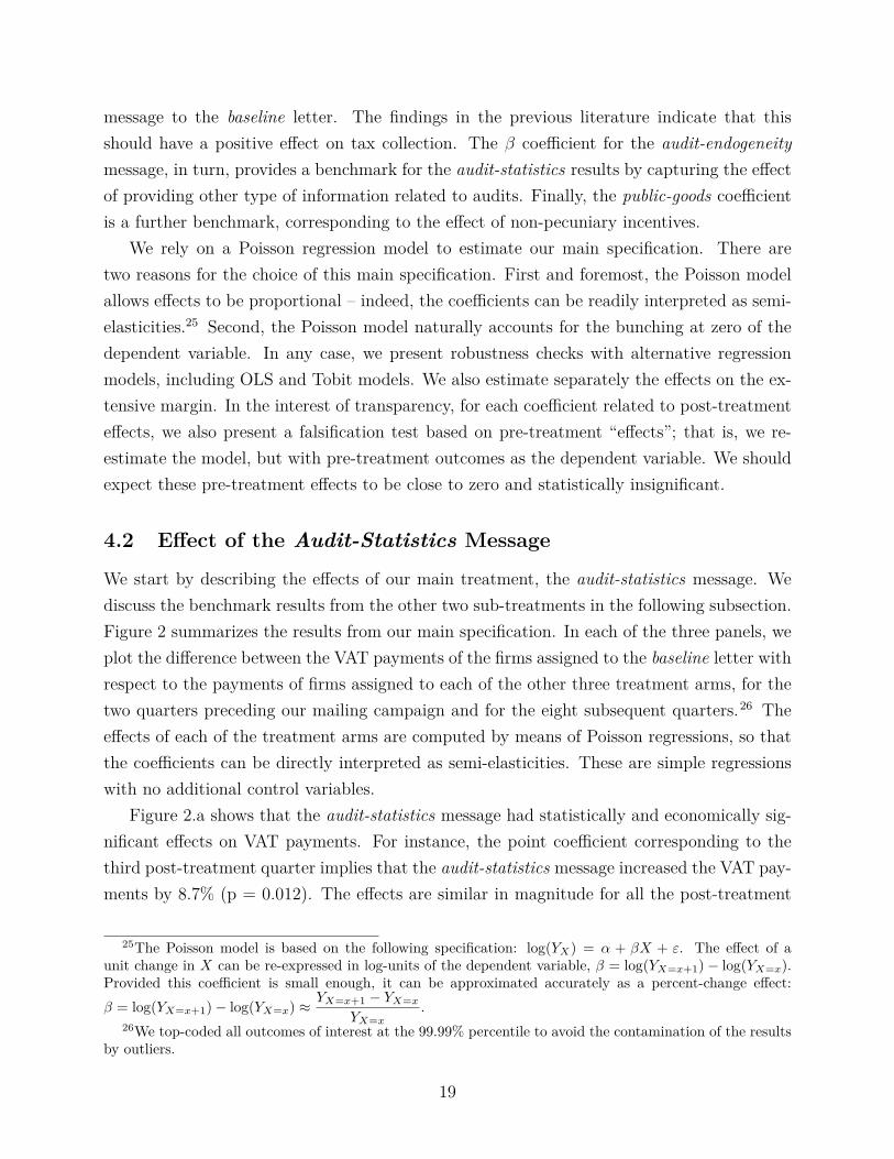
message to the baseline letter. The findings in the previous literature indicate that thisshould have a positive effect on tax collection. The β coefficient for the audit-endogeneitymessage, in turn, provides a benchmark for the audit-statistics results by capturing the effectof providing other type of information related to audits. Finally, the public-goods coefficientis a further benchmark, corresponding to the effect of non-pecuniary incentives.

We rely on a Poisson regression model to estimate our main specification. There aretwo reasons for the choice of this main specification. First and foremost, the Poisson modelallows effects to be proportional – indeed, the coefficients can be readily interpreted as semi-elasticities.25 Second, the Poisson model naturally accounts for the bunching at zero of thedependent variable. In any case, we present robustness checks with alternative regressionmodels, including OLS and Tobit models. We also estimate separately the effects on the ex-tensive margin. In the interest of transparency, for each coefficient related to post-treatmenteffects, we also present a falsification test based on pre-treatment “effects”; that is, we re-estimate the model, but with pre-treatment outcomes as the dependent variable. We shouldexpect these pre-treatment effects to be close to zero and statistically insignificant.

4.2 Effect of the Audit-Statistics Message

We start by describing the effects of our main treatment, the audit-statistics message. Wediscuss the benchmark results from the other two sub-treatments in the following subsection.Figure 2 summarizes the results from our main specification. In each of the three panels, weplot the difference between the VAT payments of the firms assigned to the baseline letter withrespect to the payments of firms assigned to each of the other three treatment arms, for thetwo quarters preceding our mailing campaign and for the eight subsequent quarters.26 Theeffects of each of the treatment arms are computed by means of Poisson regressions, so thatthe coefficients can be directly interpreted as semi-elasticities. These are simple regressionswith no additional control variables.

Figure 2.a shows that the audit-statistics message had statistically and economically sig-nificant effects on VAT payments. For instance, the point coefficient corresponding to thethird post-treatment quarter implies that the audit-statistics message increased the VAT pay-ments by 8.7% (p = 0.012). The effects are similar in magnitude for all the post-treatment

25The Poisson model is based on the following specification: log(YX) = α + βX + ε. The effect of aunit change in X can be re-expressed in log-units of the dependent variable, β = log(YX=x+1)− log(YX=x).Provided this coefficient is small enough, it can be approximated accurately as a percent-change effect:β = log(YX=x+1)− log(YX=x) ≈ YX=x+1 − YX=x

YX=x.

26We top-coded all outcomes of interest at the 99.99% percentile to avoid the contamination of the resultsby outliers.

19

quarters during the first year (e.g, 7.8%, 5.8%, 8,7% and 5.7% in the first through fourthquarter). During the second year, the effects become smaller and less statistically significantover time. The coefficients on the pre-treatment VAT payments correspond to a falsificationtest for our experiment. As expected by the random assignment of firms to different treat-ment arms, the pre-treatment differences in VAT payments are economically small and notstatistically significant.

Table 3 presents the baseline regression results. These estimates are obtained by meansof Poisson regressions with pre-treatment controls, following the econometric specificationdescribed in Section 4.1. The first column presents the main results: the average effects ofeach of the three treatments (audit-statistics in Panel A, audit-endogeneity in Panel B, andpublic-goods in Panel C) compared to the outcomes for firms that received the baseline let-ter. The post-treatment coefficients correspond to regressions with total VAT paid in the 12months after the delivery of the letter as the dependent variable (October 2015 - September2016). Additionally, as falsification tests, the pre-treatment coefficients correspond to regres-sions with total VAT paid in the 12 months prior the delivery of the letter as the dependentvariable (September 2014 - August 2015).

The post-treatment coefficient of audit-statistics (first column, panel a.) indicates thatfirms receiving this message paid 6.3% more VAT in the 12 months after the interventionon average. This effect is not only statistically significant (p = 0.013), it is also econom-ically substantial. Using the estimated average evasion rate of 26% from Gomez-Sabainiand Jimenez (2012), the effect amounts to a reduction in the evasion rate of 24% (= 6.3%

26% ).As expected, the “effect” on pre-treatment outcomes (our falsification test) is close to zero(−0.8%), statistically insignificant, and even more precisely estimated than the correspondingpost-treatment effect.27

In terms of previous findings in the literature, the effects of our audit-statistics treatmentare not directly comparable to those of the audit message from Pomeranz (2015) because themessages differed in content, and because the two studies cover firms from different countriesand with different characteristics. Nevertheless, Table 4 from Pomeranz (2015) indicates thatthe deterrence letter in that study led to an increase in VAT payments of 7.6%, which is similarin magnitude and statistically indistinguishable from the 6.3% effect of our audit-statisticsmessage. Moreover, our results are consistent with a broader literature that finds effects ofmessages about enforcement on tax compliance in a variety of contexts: self-employed incomein the United States (Slemrod et al., 2001), wage income taxes in Denmark (Kleven et al.,2011), individual public-TV fees in Austria (Fellner et al., 2013), individual municipal taxes

27The standard error on the pre-treatment coefficient is 0.021, which is smaller than the correspondingstandard error of 0.025 for the post-treatment coefficient.

20

in Argentina (Castro and Scartascini, 2015), an individual church tax in Germany (Dwengeret al., 2016), and U.S. tax delinquencies in the United States (Perez-Truglia and Troiano,2018).

The second column in Table 3 replicates the analysis for the second year after the treat-ment, i.e. October 2016 - September 2017. For this period, the effect of the treatment isless than half than that of the first year, and it is not statistically significant, even thoughthe precision of the estimate is similar in the two time periods. This is consistent with thepattern of effects by quarter depicted in Figure 2.a, which shows that the effects in the sec-ond year fall substantially when compared to those of the first year. These results are notunexpected. Over time, individuals may forget the information conveyed by the letter, or itmay become less salient. Individuals may also update their beliefs and perceptions for otherreasons, for instance because of new events such as audits and information campaigns. Thisis consistent with previous evidence on the effects of tax enforcement messages. Figure 2 inPomeranz (2015) shows that the effects of the main information campaign in that study werealso substantially higher in the first 12 months after their intervention, and fell substantiallyand became virtually zero in the 18th month (the last plotted result in the Figure).

Table 3 also presents results for complementary outcomes. As discussed in the previoussection, firms in Uruguay make payments for their current liabilities, but also for taxes thatcorrespond to previous periods — because they owe past taxes, because they revise theiraccounts and correct past mistakes, or because they impute invoices that were not availableat the time of the original payment. When firms that engage in tax evasion face a heightenedthreat of being audited, we can expect them to increase their tax payments (reduce theirevasion) in the future, but we can also expect them to retroactively revise their payments forprevious time periods to reduce or eliminate their past evasion. We explore this possibilitywith the results presented in columns (3) and (4) of Panel a in Table 3, which split the effectsof our treatment arms on retroactive and concurrent payments. These results correspondto the first year after the treatment. The messages about audits had an economically andstatistically significant effect on retroactive payments. Indeed, because of the much lowerbaseline rate, the effects on retroactive payments are larger in magnitude than the effects onthe concurrent payments. For instance, the effect for audit-statistics message is 38.1% (p =0.004) for the retroactive payments and 4.4% (p = 0.087) for the concurrent payments.

We have so far established that firms in the audit-statistics treatment arms increasedtheir VAT payments compared to recipients of the baseline letter. Our analysis focuses onVAT liabilities, which represents the largest fraction of tax payments by firms in our sample/However, our letters referred to taxes in general and did not mention VAT nor any otherspecific tax. Given the presence of other tax liabilities, the effects we reported on VAT may

21

not represent a net increase in tax payments: firms may increase their evasion (i.e., reducetheir payments) of other taxes they are liable for, crowding out payments or substitutingevasion. The results in columns (5) and (6) of Table 3 shed light on these issues. Column(5) presents the effect on all other taxes paid (mostly the corporate income tax): the effectson payments of other taxes are as economically and statistically as significant as those onVAT payments: the audit-statistics had an effect of 7.7% (p = 0.038) on other tax payments.Column (6) shows that the results are robust if we look at the effects on the sum of VAT andother taxes: the audit-statistics message increased this outcome by a statistically significant5.2%.

4.3 Benchmarks to the Audit-Statistics Message

Our research design allows us to compare the effects of the audit-statistics message to theeffects of two alternative messages, one related to audits (audit-endogeneity) and another notrelated to audits nor other forms of enforcement (public-goods).

Figure 2.b shows that the audit-endogeneity treatment arm also induced a significantchange in VAT payments compared to the baseline letter. The quarterly effect of adding theaudit-endogeneity message is positive and statistically significant in the first post-treatmentyear, and ranges between 10% and 12.4%. These effects are slightly higher than those ofthe audit-statistics treatment arm, but these differences are not statistically significant atstandard levels. As in the case of the audit-statistics message, the effects of the audit-endogeneity treatment are persistent over the first year, but diminish over the second post-treatment year. The results of the falsification test are also similar to the ones observed in theaudit-statistics treatment: the differences for the two pre-treatment quarters are economicallysmall and not statistically significant for the audit-endogeneity treatment arm.

This overall pattern of results is confirmed by the regression results presented in Panel bin Table 3. The coefficient in the first column indicates that the audit-endogeneity messageincreased subsequent VAT payments by 7.4% (p = 0.021), with no “effect” on pre-treatmentoutcomes, as expected. The effect during the first post-treatment year is similar in magnitudeto the 6.3% effect of our audit-statistics message (the difference is not statistically significantat standard levels). The effects over the second post-treatment year are also consistentwith those of the audit-statistics message: the coefficients for the second year are smaller inmagnitude than those for the first year, and they are not statistically significant. The audit-endogeneity message also had an economically and statistically significant effect on bothretroactive (31.4%) and concurrent payments (6.1%), as in the case of the audit-statisticsmessage. Finally, the results in columns (5) and (6) of Table 3 indicate that, again as in the

22

case of the audit-statistics message, the audit-endogeneity message did not crowd out othertax payments: it increased non-VAT tax payments by 8.4%.

We now turn to the effects of the public-goods treatment arm. Figure 2.c indicates thatadding this message to the baseline letter did not affect VAT payments as consistently as thetwo other treatments. While there are differences in post-treatment VAT payments betweenfirms assigned to the public-goods letters and those assigned to the baseline letter, inspectionof coefficients over time reveals that the differences in the post-treatment period were similarto the differences in the pre-treatment period.

Given these pre-treatment differences, the assessment of the effect of the public-goods mes-sage requires us to control for them. This is presented in Panel c in Table 3. The effect forthe first year of the post-treatment period as a whole for the public-goods message is positiveat 4.3%, and falls to 0.6% in the second year, and neither of these two coefficients are sta-tistically significant at standard levels (p-values of 0.147 and 0.879 respectively). Comparedto the other two treatment arms, these effects are smaller, but due to the lack of precisionthey are statistically indistinguishable. The coefficients are not statistically significant inany of the alternative specifications. The public-goods message did not have a statisticallysignificant effect either on retroactive or concurrent VAT payments (p-values of 0.304 and0.879, respectively). The effect of the public-goods message on other tax payments (column5 in Panel c in Table 3) is close to zero (0.1%) and statistically insignificant. The effectof the public-goods message on total tax payments is also small (1.8%) and statistically in-significant. Due to the precision of our estimates, we cannot rule out that the public-goodsmessage may have had some effect on tax payments. However, this findings is consistent withthe robust finding that moral suasion messages do not have significant effects on tax evasionin a variety of contexts (Blumenthal et al., 2001; Fellner et al., 2013; Castro and Scartascini,2015; Dwenger et al., 2016; Meiselman, 2018; Perez-Truglia and Troiano, 2018).28

Appendix B.2.1 presents some additional robustness checks, including regression resultsbased on alternative specifications such as OLS, Tobit and Probit models, as well as focusingon the extensive margin, and using an alternative independent source of administrative data.We show that the main findings are qualitatively and quantitatively similar to those presentedin this section, and thus robust to these alternatives.

28There are some exceptions in the literature, such as the effect of displaying norms on the timing of taxpayments (Hallsworth et al., 2017).

23

5 Tests of A&SThe results presented in the previous section are broadly consistent with the evidence in theprevious literature: providing information about audits significantly increased tax compli-ance. In this section, we present additional evidence to establish whether the effects of theaudit-statistics treatment are driven by the A&S mechanism. The subsections below presentthree different tests of A&S.

5.1 First Test of A&S: Effects on Perceptions

According to A&S, the audit-statistics message should have a positive effect on tax complianceif it increased the perceived probability of being audited, the perceived value of the evasionfine, or both. We explore this hypothesis based on data from our post-treatment survey.This survey data consists of 365 firms in the audit-statistics group and 137 in what we referto as the pooled control group with individuals who did not receive information related toaudits.29

Figure 3.a and 3.b depict the distributions of perceptions about audit probabilities andpenalty rates, respectively, as elicited from the survey. The shallow bars with solid borderscorrespond to the perceptions of firms that received the audit-statistics message. The shadedgray bars depict the distribution of perceptions for individuals from firms in the pooled controlgroup. The red dashed curve, in turn, corresponds to the distribution of signals sent to firmsin the audit-statistics letters. The comparison between the shaded bars and the red curvefrom Figure 3.a suggests that, on average, respondents in the control group substantiallyoverestimated the probability of being audited. While our administrative data on auditsindicates a probability of about 11.7%, the mean perception for the control group is 40.7%(p-value < 0.01 for the difference). This finding of overestimation of audit probabilities isconsistent with prior survey evidence (Harris and Associates 1988; Erard and Feinstein 1994;Scholz and Pinney 1995).30

Moreover, survey participants reported being confident on their responses even thoughtheir estimates were substantially off: only 16.2% of those in the control group reported being

29The survey sample size was substantially smaller than that of our experimental sample. To increasethe statistical power of our test, we defined this control group by pooling subjects from the baseline andthe public-goods groups, since both received messages with no specific information about audit probabilitiesor fines. Appendix B.3.1 shows that the results are similar, but less precisely estimated, when we only userecipients of the baseline letter for the control group.

30However, the prior survey evidence was based on responses from wage-earners, for whom the mispercep-tion of audit probabilities is mostly inconsequential due to widespread third-party reporting (Kleven et al.,2011). On the contrary, the financial stakes of misperceiving audit probabilities can be substantial in ourcontext.

24

“Not sure at all” about their perceived probability of audit (on a four point scale, rangingfrom “Not sure at all” to “Very confident”).31 Indeed, even for the subgroup of individualsfrom the control group who reported to be “Very confident” about their guesses, their averagebelief was, if anything, slightly more biased: 42.1%, still substantially higher than the actualprobability of 11.7%.

Conversely, the comparison between the shaded bars and the red curve from Figure 3.bsuggests that the average belief about the penalty rates was unbiased: the actual averagepenalty computed from administrative data for the experimental sample is 30.7%, while themean perceived penalty is 30.5% in the control group.

The positive bias in the perceived audit probability can be explained by the availabilityheuristic bias (Kahneman and Tversky, 1974). According to this model, individuals judgethe probability of an event by how easily they recall instances of it. Even though audits arerare, the fact that they may be visible for colleagues and even sometimes salient in the mediamay induce firms to perceive them to be more frequent than they actually are. Indeed, thereis evidence that individuals overestimate the probabilities of a wide range of rare events of asimilar nature (Lichtenstein et al., 1978; Kahneman et al., 1982).

The systematic upward bias in perceptions of audit probabilities and the results presentedin the previous section, showing that the audit-statistics message increased tax compliance,are not consistent with A&S. Since our letters provided information about audit probabil-ities that was lower than firms’ beliefs, the A&S framework would predict a reduction taxcompliance. Our post-treatment survey allows us to test this hypothesis more directly. Fromthe assignment of firms to the different treatment groups, we can measure the effect of theaudit-statistics letter on the perceived p and θ. The shallow bars with solid borders in Figures3.a and 3.b depict the distribution of perceptions for respondents from firms in the audit-statistics treatment arm. Inspection of Figure 3.a indicates that, compared to respondentsin the treatment group, recipients of the audit-statistics message reported on average a lowerperceived probability of being audited, from an average of 40.7% in the pooled control groupto an average of 35.2% in the audit-statistics group (p-value of the difference 0.03). Mean-while, Figure 3.b shows that the audit-statistics message had a small effect on the perceivedpenalty rate, decreasing it from an average of 30.5% for the pooled control group to an aver-age of 29.9% for the audit-statistics group, with this difference being statistically insignificant(p-value of 0.85).

This analysis only provides a lower bound for the effect of our letters on perceptions.While we are confident that our certified letters reached firms’ owners, we cannot be asconfident about whether the owner was the same person who received the email invitation

31A similar share (18.1%) reported to be “Not sure at all” about their guess for the penalty rate.

25

to complete the survey. Moreover, the survey responses took place over nine months afterour letters were sent, so it is feasible that recipients had forgotten the mailing’s messagesat that point, or that they had acquired additional information in the meantime. Thus, thetrue effect of the audit-statistics on the average subjective audit probability was probablyeven more negative than what we report above.

To sum up, the evidence suggests that the audit-statistics treatment arm may have re-duced the average perceived audit probability. This evidence, and the positive effects of thistreatment on tax compliance, are jointly inconsistent with A&S , according to which thismessage, by reducing perceived audit probabilities, should have reduced tax payments. Con-sistent with this evidence, Appendix B.3.2 suggests that the effect of the audit-endogeneitymessage is not due to an update of recipients’ beliefs about the degree of endogeneity of auditprobabilities, because recipients were already well aware of this endogeneity.

One important caveat for this test and those we present in the following subsections isthat our analysis relates to the behavior of the average firm. While the average firm doesnot behave as A&S predicts, we cannot rule out that some of the firms behave in a mannerconsistent with A&S. In other words, it is possible that some firms updated their perceivedprobability upwards because of the information contained in the letter and increased theirtax payments as a consequence.

Another caveat with this test is that it is based on survey data, which has some limitations.However, we can address some of those challenges. A first concern is that our subjects maybe confused about the meaning of an “audit.” However, our survey data provides directevidence on the contrary. Among the 145 responses from the pooled control group, 10.3%of firms reported that they were audited in the past three years. Since this share (10.3%)is close to the actual share of firms that were audited (11.7%), it seems that respondentsunderstood the definition of an audit correctly.

A second concern with survey data is that subjects may have difficulties responding aboutpercentages and probabilities. However, this may be a less of a concern in our subject pool,which is comprised of business owners who should be familiar with fractions and probabilities.At the very least, they need some rudimentary arithmetic and understanding of percentagesto compute the VAT and other tax liabilities.

A last source of concern with our survey data is that, in some circumstances, respondentsmay report probabilities of exactly 50% as a way of expressing their uncertainty (Bruinet al., 2002; Bruine de Bruin and Carman, 2012). Responses of exactly 50% are somewhatcommon in our data: among individuals in the pooled control group, 33.3% of responsesabout the perceived audit probability and 16.4% of responses about the penalty rate areexactly equal to 50%. To assess the extent of this concern, we follow the standard method

26

from Bruin et al. (2002) and Bruine de Bruin and Carman (2012). We measure certaintyusing a 1-4 scale from “Not sure at all” (1) to “Very confident” (4). If there were largedifferences in certainty between individuals who responded exactly 50% and the rest, thatwould cast doubts on the validity of the survey responses. On the contrary, we find modestdifferences in certainty between the two groups.32 As a complementary robustness check, wecan conduct our analysis ignoring 50% responses and treating them as missing data. Evenwith this conservative approach, individuals in the control group still substantially over-estimate the probability of being audited: these respondents report an average perception of31.5%, compared to the actual probability of 11.7%.

In the following sections, we provide alternative tests of A&S that do not rely on surveydata.

5.2 Second Test of A&S: Heterogeneity with Respect to Signals

5.2.1 Reduced-Form Results

The second test is based on the differential effects of the values of the signals provided in theletters. According to A&S, the effects of the audit-statistics message should be increasing inthe signals about the audit probability (p) and the penalty rate (θ). The random variationwe introduced in the p and θ conveyed in our audit-statistics letters allow us to test thishypothesis directly. Figure 4 starts with a less parametric look at the data. This figureuses the main specification from before,33 looking effect of the audit-statistics message onVAT payments, but broken down by decile of the signals included in the letter. Figure 4.apresents the effect of the audit-statistics message by decile of the signal of p included in theletter. In the A&S framework, we should expect that very low signals of p should reduce taxcompliance (since they most likely reduce the firms’ perceived probability of audits), whereasthe effect should become larger, and turn positive at some point, as we increase the value ofthe signal about p.

The coefficients plotted in Figure 4.a, however, indicate that the effect of the audit-statistics letter is not related to the value of p included in the letter. The coefficients aresimilar in magnitude for the whole range of values from p = 2% all the way up to p = 25%.For example, the effect is 8.8% and statistically significant (p-value of 0.016) for the lowest

32In the pooled control group, the average certainty for perceived audit probability is 2.18 for individualswho responded a value of exactly 50%, and 2.56 for individuals who responded a different value (p-valueof difference 0.09). For the responses about the perceived penalty rate, the average certainty is 2.18 forindividuals who responded 50%, and 2.48 for those who responded another value (p-value of difference 0.35).

33Additionally, we control for dummies for the quintiles of pre-treatment VAT payments, from which wedrew the sample to calculate pi and θi.

27

decile (p ∈ [2%, 5%]), and it is 5.6% and marginally significant (p-value of 0.065) for firms inthe upper decile (p ∈ [19%, 25%]). Moreover, the resulting slope (in dashed red line), whilepositive as predicted by A&S, is economically small (0.0014) and statistically insignificant(p-value=0.637).

Figure 4.b provides an analysis similar to that of Figure 4.a, but instead of looking atthe heterogeneity by audit probabilities (p) it shows the heterogeniety by penalty rates (θ).According to A&S, we should expect a positive relationship between the effect of the audits-statistic letter and the value of θ included in the letter. Figure 4.b shows evidence to thecontrary: the coefficients are similar for the whole range of values from θ = 15% to θ = 68%,with the slope being negative, economically small and statistically significant.

One potential confounding factor for our findings about the lack of effect of variations inp and θ is that some subjects might have interpreted the audit-statistics message per se as asignal that their firms were under the IRS radar, above and beyond the factual informationconveyed in the message. We were careful to mitigate this concern in the design of ourmailings. For instance, we highlighted the fact that the letter recipients were randomlyselected. Nevertheless, some individuals may have ignored or overlooked this cue. However,even if the recipients learned something from the receipt of the audit-statistics message, thereis no reason why they should not learn about the content of the message as well. In otherwords, the test presented above continues to be valid, as A&S would still predict that theaudit-statistics message should have a differential effect depending on the values of p and θ.

To address this concern more directly, we use the audit-threat treatment arm, in which thetax agency made an explicit threat to every recipient and thus is not subject to this concern.Figure 5 depicts the difference in the evolution of VAT payments over time between the twosub-treatments in the audit-threat arm, corresponding to audit probabilities of 50% and 25%.We find no systematic difference between the two groups in post-treatment VAT payments.This complementary test further reinforces the result that, contrary to the prediction of A&S,tax compliance does not depend on the exact probability being audited.

5.2.2 Elasticities with respect to p and θ

For a more direct test of A&S, we can quantify the effects of the audit-statistics and audit-threat sub-treatments in a way that can be contrasted to the quantitative predictions of A&S.For the audit-statistics treatment arm, we use the following model:

Yi = α + γp · pi + γθ · θi +5∑g=2

πg · I{i∈g} +Xiδ + εi (2)

28

where pi ∈ (0, 1) is the signal about the audit probability included in the letter sent to subjecti, and θi ∈ (0, 1) is the signal about the penalty rate included in the letter sent to the samefirm. The I{i∈g} variables correspond to a set of dummies for quintiles of pre-treatment VATpayments, which are the groups from which we drew the sample of “similar firms” to calculatepi and θi. Including these controls ensures that we only exploit the exogenous variation inpi and θi induced by our experimental design – that is, the heterogeneity due to samplingvariation. Since we are using a Poisson regression model, γp and γθ can be directly interpretedas elasticities. For instance, an estimate of γp = 1 would imply that a 1 percentage pointincrease in the audit probability conveyed in the letters increased VAT payments by 1%.From A&S , we can expect that γp > 0 and γθ > 0 – i.e., firms tax payments are increasingin the perceived probability of audit and evasion penalty rates. Moreover, we can comparethe values of these regression estimates to the predictions from calibrations of A&S.

A similar econometric model can be used for firms assigned to the audit-threat letter:

Yi = α + γp · pi +Xiδ + εi (3)

where pi ∈ {0.25, 0.50} is the audit probability included in the audit-threat letter sent to firmi. As in the previous regression, A&S implies a positive estimate of γp.

Panel (a) in Table 4 presents the results from the econometric model of equation 2. Col-umn (1) of Table 4 presents estimates of the elasticities of VAT payments with respect to thevalues of p and θ conveyed in the audit-statistics sub-treatments. The elasticity with respectto the audit probability in the first year after the treatment is 0.030 (SE of 0.236, p-value of0.897). This means that increasing p by 1 percentage point would increase VAT payments bya mere 0.03%. The elasticity with respect to the penalty rate is −0.118 (SE 0.115, p-value of0.304), which implies that increasing θ by 1 percentage point would reduce VAT paymentsby 0.118%. The estimates are close to zero, not statistically significant at standard levels andprecisely estimated. The precision implies that we can rule out even moderate elasticities:the 90% confidence interval for the audit probability excludes elasticities above 0.418, andthe 90% confidence interval for the penalty rate excludes elasticities above 0.071.

It should be noted that the pre-treatment falsification test does not yield any statisticallysignificant effect, and that the results are similar (no statistically significant elasticities) forthe other specifications: for the second year (column (2)), by timing of the payment (columns(3) and (4)), and by type of tax (columns (5) and (6)). In most cases, the estimates are notstatistically significant. There are some exceptions, such as the coefficient associated with theaudit probability for retroactive payments, but in this case the differences were statisticallysignificant before the treatment too, and therefore this result is probably spurious.

As complementary evidence, panel (b) of Table 4 presents the results of the audit-threat

29

treatment arm in regression form, following the econometric model of equation 3. Whilethe audit-threat messages implies an elasticity with respect to p of 0.376, this estimate onlyborderline significant at the 10% level (p-value of 0.073) and economically small. Moreover,the pre-treatment (falsification) coefficient (-0.342) is also borderline statistically significantat the 10% level (p-value of 0.055), indicating that the small post-treatment effect may bespurious.

Appendix B.2.3 present a series of robustness checks (alternative specifications basedon OLS, Tobit and Probit models, and using an alternative data source for the dependentvariable), and the results are similar. An additional robustness check, presented in the sameAppendix, shows that results are robust if, instead of estimating the elasticities with respectto p and θ separately, we estimate the elasticity with respect to p ∗ θ (i.e., the expectedpenalty per dollar evaded).

Taken together, this evidence suggests that firms did not react to the values of the pa-rameters conveyed in our letters. Since we devoted a large fraction of our subject pool tothis treatment arm, these elasticities are quite precisely estimated.

Moreover, we can assess the economic magnitude of these differences by benchmarkingthese elasticities with the quantitative predictions of A&S. The exact predictions of A&Sdepend on the specific model at hand and on the values of the underlying parameters. Weprovide calibrations under a number of settings that have been considered in the literature,allowing for social preferences (Luttmer and Singhal, 2014), endogenous audit probabilities(Allingham and Sandmo, 1972; Yitzhaki, 1987), misperceptions about audit parameters (Almet al., 1992) and non-audit detection (Acemoglu and Jackson, 2017). We calibrate differentcombinations of these models to match the average VAT evasion rate in Uruguay (26%, asestimated by Gomez-Sabaini and Jimenez, 2012), and compute the elasticity of tax paymentswith respect to p and θ under each of the alternative calibrations.

The details and results from these calibrations are presented in Appendix C. Since allthe different calibrations lead to elasticities in the same order of magnitude, the results aresimilar regardless of the calibration that we use. In our preferred calibration, we find anelasticity of tax payments with respect to the audit probability of 4.55, and an elasticityof tax payments with respect to the penalty rate of 3.48. We can test the null hypothesisthat the elasticities with respect to p and θ in the main specification of the audit-statisticspresented in column (1) of Table 4 are equal to those in our preferred A&S calibration. Wecan reject the null that the elasticity is 4.55 for the audit probability, and that it is 3.48 forthe penalty rate (both tests with p-values<0.001). These calibrated elasticities are also wellbeyond the confidence intervals for the coefficients estimated for the audit-threat model.

It should be noted that our discussion is based on the implicit assumption that a letter

30

conveying the message of a 1 percentage point higher signal of p or θ will increase theperception of the parameter by the recipient by 1 percentage point. This is probably astrong assumption: some individuals may not have read the letter in its entirety, they mayhave not entirely believed in the content of our message, or may not have updated theirprior by the full value of the signal. For a benchmark, we can compare our setting withstudies of learning from economic variables, such as the inflation rate (Cavallo et al., 2017),the cost of living (Bottan and Perez-Truglia, 2017), and housing prices (Fuster et al., 2018).These studies find that for each percentage point increase in the feedback given to subjects,the average individual updates beliefs about half a percentage point. If we assume thisrate of learning, then we should double the elasticities estimated in our regressions beforecomparing them to the calibrations of A&S. Under this assumption, we can still reject thenull that the estimated and the calibrated elasticities of tax compliance with respect to theaudit probability are equal (p-value<0.001 for each γp and γθ ).

Since we have survey data on the audit-statistics group, we can estimate the learningrate directly. However, this exercise faces two significant challenges. First, we elicited thesebeliefs with a survey conducted nine months after the information was provided, so the effectof the information may have decayed substantially. For example, Cavallo et al. (2017), showsthat the effect of information on beliefs decays by about half in a matter of just three months(similar findings are reported in Bottan and Perez-Truglia, 2017 and Fuster et al., 2018).The second limitation is the small sample size (365 observations). With those caveats inmind, the survey data suggests that a percentage point increase in the signal about the auditprobability provided in the letter increased the perceived audit probability nine months laterby 0.397 (SE 0.288) percentage points. This point estimate must be taken with a grain of saltbecause it is imprecisely estimated and thus statistically insignificant at conventional levels.However, it is reasurring that the point estimate suggests a learning rate that is consistentwith the learning rates from other studies used as a benchmark above.

Moreover, we can reproduce the analysis under an extremely conservative assumptionabout the magnitude of the learning rate. Even if we assumed that for each percentage pointdifference in the letter individuals only adjusted their beliefs by one tenth of a percentagepoint, we would still fail to reject the null hypothesis that the estimated elasticities are equalto those in the A&S calibration.

Our estimates are similar to those obtained in laboratory experiments. For example, Almet al. (1992) find an elasticity with respect to the audit probability of 0.169 (comparableto our estimate of 0.030), and with respect to the penalty rate of 0.037 (comparable to ourestimate of -0.118). Indeed, the elasticities reported in Alm et al. (1992) are statisticallyindistinguishable from the elasticities reported in our study.

31

The findings from the audit-statistics and audit-threat arms are also consistent with someresults from other field experiments. Dwenger et al. (2016) conducted a field experiment inthe context of a local church tax in Germany for which enforcement was very lax. In one oftheir treatment arms, they included information with different probabilities of audits (p = 0.1,p = 0.2, or p = 0.5). They do not compute elasticities with respect to p that we can comparewith ours. However, consistent with our probability neglect result, the effect on increasedcompliance and increased payments is very similar (and statistically indistinguishable) forthe three treatment arms. Another related experiment, Kleven et al. (2011), included atreatment arm with two different audit probabilities. Consistent with our results, they findeconomically negligible differences in tax compliance between individuals assigned to differentaudit probabilities.34 However, the evidence from Kleven et al. (2011) is not inconsistent withA&S because, unlike in our context, their subjects face automatic third party reporting.35

5.3 Third Test of A&S: Heterogeneity with Respect to Prior Be-liefs

5.3.1 Measuring Prior Beliefs

In the A&S framework, firms with different prior beliefs about the probability of beingaudited should react differently to signals and information about this probability. To testthis hypothesis, we need a measure for prior beliefs for a particular firm. We construct aproxy of prior beliefs based on the firm’s own audit history.

The intuition behind this approach is that, since there is little publicly available infor-mation about audit probabilities, firms may form their beliefs based on their own auditexperience. For instance, when a firm registers with the tax authority, its initial belief mayfollow the beta distribution with parameters {α0, β0}. Assume that firm i has been registeredfor Ti years before our mailing campaign, and during this period it has experienced Ni ≤ Ti

audits. If firm i is Bayesian, its belief about annual probability of being audited should followa beta distribution with parameters {α1 = α0 +Ni, β1 = β0 + Ti −Ni}. The mean of thatbelief should be α0+Ni

α0+β0+Ti . In turn, this implies a belief of the probability of being audited at

34In one of their treatments, they send letters to individuals stating large audit probabilities of p = 50%and p = 100%. Compared with a group that did not receive any letter, they find that the letters had apositive and significant effect on declared income and tax liability. The differential effects between thesetwo conditions, while is statistically significant, is economically negligible: an increase in the signal aboutprobability of audit from 50% to 100% increases reported income by 0.025% and taxes paid by 0.05%.

35They conduct their experiments with wage earners, for whom evasion is automatically detected throughthird-party reporting without the need for audits. As a result, A&S predicts that, consistent with theirevidence, wage earners should report their wage incomes truthfully regardless of the probability of beingaudited (Kleven et al., 2011).

32

least once in the following three years of p̂i = 1−(1− α0+Ni

α0+β0+Ti

)3. In our main specification,

we generate these proxies setting {α0 = 0.13, β0 = 1}. This baseline calibration generates anaverage belief that matches the actual average probability in our administrative data, andwe offer robustness tests using alternative calibrations.36

We can use the survey data to validate this proxy for the prior belief. Among the 145responses from the pooled control group, 10.3% of firms reported that they were auditedin the past three years and the remaining 89.7% reported that they were not. We findthat respondents from firms that were audited in the recent past reported a higher averageperceived probability of being audited (63.9%) than individuals from firms that were notrecently audited (38.1%). This different is not only economically large, but also statisticallysignificant (p-value<0.001).37 This evidence suggests that, consistent with our proxy, firmsare using their own audit history to form beliefs about the probability of being audited inthe future.

5.3.2 Results

In the A&S framework, the effect of the audit-statistics letter on tax compliance should belarger for firms with relatively low priors for the audit probability (p̂) compared to thosewith relatively high values of p̂. More specifically, the audit-statistics conveyed, on average, asignal of p̂ = 11.7%. The effect of this message on compliance should thus have been positivefor the group with p̂ < 11.7%: i.e., on average, the signal should increase their perceived auditprobability. On the contrary, the effect of the audit-statistics message should be negative forfirms with p̂>11.7%: on average, the signal should reduce their perceive probability of beingaudited.

Figure 6 presents the results. Figure 6.a presents a binned scatterplot with the treatmenteffect of the audit-statistics letter for the four quartiles of p̂. This figure includes a verticaldashed line at 11.7%, the average message about the audit probability conveyed by our letters.In contrast to the predictions from A&S, we fail to find a negative relationship between theeffect of the audit-statistics message and the value of the prior belief: the slope is negative(-0.0213), but economically small and statistically insignificant (p-value of 0.146).

Figure 6.b presents a more direct test, which combines heterogeneity in prior beliefs with36Since we only have information about audits for firms in our sample for the previous 15 years, we set

the maximum firm age at 15 to compute these priors.37As reported in a follow-up paper (Bergolo et al., 2018), the indicator of recent audits is the single

most important predictor of perceived audit probabilities among a host of different factors. The recent auditexperience also has a positive effect on the perceived penalty rate, but this effect is less significant: respondentsfrom firms that were audited recently report an average perceived penalty rate of 40.0%, compared to 29.4%for respondents from firms that were not audited recently, although this difference is statistically insignificant(p-value of 0.201).

33

heterogeneity in signals. Instead of grouping firms by their prior beliefs, we group then bythe difference between their prior and the specific signal sent to each firm in its personalizedletter. The intuition is that the difference between the prior and the signal is the “surprise”conveyed by our information treatment. We included a vertical dashed line at 0, i.e., at thepoint were firms receive signals equal to their priors. The effect of the audit-statistics letteron compliance should be decreasing in p̂− psignal, positive for the group with p̂− psignal < 0(i.e., those for whom the signal was higher than their prior) and negative for the group withp̂ − psignal > 0 (i.e., those receiving a signal indicating that they were overestimating theaudit probability). The results in Figure 6.b are consistent with the results from Figure 6.a:the slope of the relationship (in dashed red line) is negative (-0.0129) but economically smalland statistically insignificant (p-value of 0.515).

Appendix B.2.2 shows that these results are robust to a number of checks. For instance,the results are similar if we calibrate p̂ to be centered at the average perceived audit proba-bility instead of the actual audit probability. Moreover, the results are consistent with a lessparametric version of the test, in which we simply compare the effects of the audit-statisticsmessage between firms that were audited in the past and firms that were not.

6 Discussion

Our experiment was designed to test the null hypotheses of A&S. Given that our evidencerejected these null hypotheses, it remains unclear which alternative model is best suitedto explain the findings. We consider some of these alternative models in this section. Tofacilitate the discussion, we organize the main findings in three groups:

• Increased compliance: on average, the audit-statistics message had a positive effect ontax compliance.

• Reduced subjective probability: on average, the audit-statistics message decreased theperceived probability of being audited.

• Probability neglect: the effect of the audit-statistics message did not depend on the auditprobability included in the letter nor on the firm’s prior belief about this probability.

Below we discuss the plausibility of different models:

A&S with Salience. One natural model to consider is that of salience (Chetty et al.,2009). According to this model, firms behave as if the probability of detection and thepenalty rate are zero, unless these parameters are made salient to them. This model could

34

reconcile the findings of increased compliance and reduced subjective probability: even ifthose who were sent the messages adjusted their perceived audit probabilities downwards,they would have behaved as if those probabilities were zero if they had not received thosemessages. However, the salience model fails to fit other features of our findings. First, bydefinition, salience models imply short-lived effects. A reminder about a non-salient taxshould affect the behavior of an agent only when receiving the information, but not lateron. This prediction contradicts our evidence about the persistent increased compliance fromfirms that received our audit-statistics letter. This persistence remained for months afterthe messages were transmitted. Salience models also are inconsistent with our finding ofprobability neglect (i.e., making salient a high probability of audit should have a strongerimpact than information about a low probability of audit).

A&S with Prospect Theory. It is possible to incorporate prospect theory (Kahnemanand Tversky, 1979) into A&S (e.g., Dhami and al Nowaihi, 2007). This extension of themodel, however, is unlikely to explain our findings. Most important, prospect theory isunlikely to explain our finding of probability neglect. Although differences between extremelylow probabilities can be ignored under prospect theory, the range of probabilities in ourcontext was far from what is normally considered extremely low (e.g., in the audit-threatarm, the probabilities were 25% versus 50%).

Risk-as-feelings. Our preferred interpretation is based on the model of risk-as-feelings(Loewenstein et al., 2001). The models used for choice under uncertainty are typically cogni-tive, in the sense that agents make decisions using some type of expectation-based calculus.The risk-as-feelings model proposes that responses to fearsome situations may differ substan-tially from cognitive evaluations of the same risks (Loewenstein and Lerner, 2003).38 Whenfear is involved, the responses to risks are quick, automatic, and intuitive, and they tendto neglect the cost-benefit calculus. A key prediction of this model is that feelings aboutrisk will be mostly insensitive to changes in probability, which is known in the literature asprobability neglect (Sunstein (2002); Zeckhauser and Sunstein, 2010), or the fear that makesindividuals focus on the downside of outcomes and thus ignore the underlying likelihoods.There is evidence of probability neglect in a range of fearsome situations involving electricshocks, arsenic, abandoned hazardous waste dumps, pesticides, and anthrax (Sunstein (2003);Zeckhauser and Sunstein, 2010).

38A related concept, the affect heuristic, corresponds to the quick, automatic and intuitive evaluations ofrisky situations based in emotions, which might be used as shortcut for more complex evaluations of risk(Slovic et al., 2004). Borrowing Kahneman (2003) terminology for the dual system model of the human mind,emotions might influence the intuitive system.

35

This model of risk-as-feelings can reconcile all of our key findings. It explains the findingof probability neglect, as well as the findings of increased compliance and reduced subjectiveprobability. Even if the perceived probability of an audit decreased among the treatmentsubjects, they still may be scared into paying more taxes, because they did not rely oncognitive evaluations of probabilities anyway. Our interpretation suggests that taxpayersoverreact to the threat of audits. In other words, audits may scare taxpayers into compliancein the same way that scarecrows scare birds. Indeed, beyond tax compliance, fear has beenfound to drive excessive caution in other contexts (Loewenstein et al., 2001).39

There is some evidence that individuals may have an emotional reaction when dealingwith tax audits and, more generally, the tax authority. A survey by the United States InternalRevenue Service (2018) indicates that 61% of U.S. taxpayers consider “fear of an audit” tohave significant influence on their tax compliance decisions.40 This is also reflected in thepopular press. For example, a The Washington Post (2016) article claims that “a lot ofpeople are super scared of the Internal Revenue Service” and that its powers “can instill alot of fear.” The fear of the tax authority can be extreme enough to be considered a phobia(New York Times, 2009). Laboratory experiments also have confirmed the role of fear intax compliance. Coricelli et al. (2010) conducted a fairly typical tax evasion game in thelaboratory and measured how emotional arousal affected tax evasion decisions. They showedthat the intensity of emotional arousal predicts whether individuals evade and by how much.In a related laboratory setting, Dulleck et al. (2016) showed a significant correlation betweentax compliance and physiological markers of stress during the tax reporting decision.

In other areas of public policy, the risk-as-feelings heuristic can be a problem, because itdistorts facts and promotes irrational judgment, leading to suboptimal decisions from a purerisk-assessment perspective. For example, Zeckhauser and Sunstein (2010) and others discusscases involving regulation of nuclear power, vaccines, and other emotion-arousing issues.

For tax collection, these emotional biases might have positive implications, at least fromthe tax authority’s perspective. In fact, some anecdotal evidence suggests that tax authoritiesuse the risk-as-feelings model to foster tax compliance. In the United States, for example,a disproportionately large number of tax enforcement press releases covering criminal con-victions and civil injunctions are released during the weeks immediately preceding Tax Day,presumably to scare taxpayers into preparing compliant returns (Morse, 2009; Blank and

39For example, fear to terrorist attacks can make people choose other, more dangerous forms of transport;and fear of shark attacks can lead to unnecessary legislation (Sunstein, 2002, 2003; Zeckhauser and Sunstein,2010).

40More precisely, 32% of respondents claim that “fear of audits” exert “a great deal of an influence” and29% “somewhat of an influence” in whether they honestly report and pay their taxes. In comparison, auditsare perceived to be as strong of a deterrent as third-party reporting: 66% of respondents stated that “thirdparty reporting (e.g., wages, interest, dividends)” influence their tax compliance.

36

Levin, 2010). Moreover, some tax experts claim that the IRS “likes [targeting] celebritiesbecause they get the most bang for their buck in terms of publicity” to “scare the public intocomplying” (Forbes, 2008).

Furthermore, the risk-as-feelings framework indicates that vivid imagery can effectivelyinstill fear and biases in risk evaluations (Slovic et al., 2004; Zeckhauser and Sunstein, 2010).Coincidentally, tax agencies seem to resort to vivid images in some of their advertising cam-paigns. For example, in the United Kingdom, the tax agency posts banners in all sorts ofpublic spaces. One of those banners, reproduced in Figure 7, shows a pair of eyes peekingthreateningly through a gash in the paper. The poster reads, “If you’ve declared all your in-come you have nothing to fear.” The tax authority in Formosa, Argentina, was perhaps evenless subtle: its ad campaign starred a monster kidnapping tax evaders and individuals in ar-rears with their taxes.41 The tax authority claims that the use of the monster was supposedto be humorous, but they also may have been trying to send a subliminal message (Clarin,2016). Similarly, a TV advertisement in the United States showed the IRS as “somethinglike poltergeist coming out of a TV set and the world falling apart,” followed by the phrase,“Have you filed your income tax?” (United Press International, 1988).

These campaigns and anecdotes suggest that some tax administrations may be leveragingfear for tax collection. Even if administrations leverage existing fear rather than instill it,relying on such tactics is not obvious from a normative perspective, since the ethics of suchcampaigns could be questionable. Moreover, actively promoting fear could have unintendednegative effects, such as imposing negative psychological stress on taxpayers. 42

7 Conclusions

The canonical model of Allingham and Sandmo (1972) predicts that firms evade taxes byoptimally trading off between the costs and benefits of evasion, but it is unclear whetherreal-world firms react to audits in this way. We designed a large-scale field experimentin collaboration with Uruguay’s tax authority to assess the factors behind firms’ evasionbehavior and their reactions to audits. Our findings indicate that firms do increase their taxcompliance when informed about the auditing process. However, we do not find this reactionto be consistent with the predictions of A&S. For example, the information about auditsdecreased (rather than increased) the perceived probability of being audited; also, the effectsof our messages about audit probabilities were independent of the signal we conveyed and

41They used an aboriginal mythical monster, the “Pombero,” a sort of boogeyman that according tofolklore took away misbehaving children.

42For a discussion on the ethical and practical issues with the use of communication efforts to increase taxcompliance, see for example Morse (2009).

37

of the firms’ prior beliefs. Models of salience are consistent with the increased compliancewe observed and with the reduced perceived perception of audit probabilities, but they arenot consistent with our findings of probability neglect. We argue that all three findings canbe reconciled by the risk-as-feelings model, which highlights the role of emotions in decision-making and which predicts that agents might exhibit probability neglect in dreaded or fearedsituations, like paying taxes.

We conclude by discussing some policy implications. In the traditional framework of A&S,the relevant policy lever is the number of audits: the tax agency must find the point at whichthe marginal cost of an additional audit equals the expected marginal benefit (i.e., highertax revenues). Our findings suggest that small and medium firms face significant informationand optimization frictions when reacting to audits. These frictions introduce new levers forpolicy-making. For example, tax agencies can decide whether to be transparent about theauditing process,43 whether to contact taxpayers to remind them of the auditing process,and whether to make the costs of being a tax cheat salient and vivid through advertisementcampaigns.44 Indeed, we discussed anecdotal evidence that some tax agencies may alreadyhave a working knowledge of these new policy levers. For example, some tax agencies seemto avoid transparency about the auditing process while increasing visibility of enforcementactions around tax day. Some even refer to fear in their advertisement campaigns. However,there is no direct evidence on whether these policies effectively increase tax compliance orwhether they have unintended effects, such as instigating enough fear in taxpayers to makethem so anxious and unhappy that it trumps the positive effects of tax revenues. As statedby Alm (2019), in a recent review of the literature, “the role of emotions in tax compliancedecisions remains largely unexamined.” Our results highlight the need for more research onprobability neglect in the decision to pay taxes. Moreover, additional research should examinethe role of emotions on other important economic choices beyond tax compliance.

43On the one hand, our evidence indicates that increasing transparency about the audit probability wouldreduce the average perceived probability of being audited, which could in turn reduce tax compliance. Onthe other hand, our finding of probability neglect suggests that, in the end, the reduction in perceived auditprobability may not affect tax compliance.

44For a practical discussion on how to implement this type of policy, including the drawbacks, see Morse(2009). Furthermore, this same principle can be used to improve compliance with other laws. For instance,Dur and Vollaard (2019) show experimental evidence that salience of tax enforcement can be used to reduceillegal garbage disposal.

38

ReferencesAcemoglu, D. and M. O. Jackson (2017). Social Norms and the Enforcement of Laws. Journal of

the European Economic Association 15 (2), 245–295.

Allingham, M. G. and A. Sandmo (1972). Income Tax Evasion: A Theoretical Analysis. Journalof Public Economics 1, 323–338.

Alm, J. (2019). What motivates tax compliance? Journal of Economic Surveys 33 (2), 353–388.

Alm, J., B. Jackson, and M. McKee (1992). Estimating the Determinants of Taxpayer Compliancewith Experimental Data. National Tax Journal 45 (1), 107–114.

Alm, J., G. H. McClelland, and W. Schulze (1992). Why do people pay taxes? Journal of PublicEconomics 48 (1), 21–38.

Becker, G. S. (1968). Crime and Punishment: An Economic Approach. Journal of Political Econ-omy 76 (2), 169–217.

Bergman, M. and A. Nevarez (2006). Do Audits Enhance Compliance? An Empirical Assessmentof VAT Enforcement. National Tax Journal 59 (4), 817–832.

Bergolo, M., R. Ceni, G. Cruces, M. Giaccobasso, and R. Perez-Truglia (2018). Misperceptionsabout Tax Audits. AEA Papers and Proceedings 108, 83–87.

Blank, J. D. and D. Z. Levin (2010). When Is Tax Enforcement Publicized? Virginia Tax Review 30.

Blumenthal, M., C. Christian, and J. Slemrod (2001). Do Normative Appeals Affect Tax Com-pliance? Evidence From a Controlled Experiment in Minnesota. National Tax Journal 54 (1),125–138.

Bottan, N. L. and R. Perez-Truglia (2017). Choosing Your Pond: Location Choices and RelativeIncome. NBER Working Paper (23615).

Bruin, W. J. A. B. d., P. S. Fischbeck, N. A. Stiber, and B. Fischhoff (2002). What number is"fifty-fifty"? Redistributing excess 50% responses in risk perception studies. Risk Analysis 22 (4),725–735.

Bruine de Bruin, W. and K. G. Carman (2012). Measuring Risk Perceptions: What Does theExcessive Use of 50% Mean? Medical Decision Making 32 (2), 232–236.

Castro, L. and C. Scartascini (2015). Tax Compliance and Enforcement in the Pampas EvidenceFrom a Field Experiment. Journal of Economic Behavior & Organization 116, 65–82.

39

Cavallo, A., G. Cruces, and R. Perez-Truglia (2017, July). Inflation Expectations, Learning, andSupermarket Prices: Evidence from Survey Experiments. American Economic Journal: Macroe-conomics 9 (3), 1–35.

Chetty, R., A. Looney, and K. Kroft (2009). Salience and Taxation: Theory and Evidence. TheAmerican Economic Review 99 (4), 1145–77.

Clarin (2016, September). Polemica campana en formosa al que no paga los impuestos se lo llevael pombero. Clarin.

Coricelli, G., M. Joffily, C. Montmarquette, and M. C. Villeval (2010). Cheating, Emotions, andRationality: An Experiment on Tax Evasion. Experimental Economics 13 (2), 226–247.

Cowell, F. A. and J. P. F. Gordon (1988). Unwillingness to pay: Tax evasion and public goodprovision. Journal of Public Economics 36 (3), 305–321.

DellaVigna, S. and M. Gentzkow (2017). Uniform Pricing in US Retail Chains. Working Paper23996, National Bureau of Economic Research.

Dhami, S. and A. al Nowaihi (2007). Prospect theory versus expected utility theory: Why DoPeople Pay Taxes? Journal of Economic Behavior and Organization 64 (1), 171–192.

Dulleck, U., J. Fooken, C. Newton, A. Ristl, M. Schaffner, and B. Torgler (2016). Tax complianceand psychic costs: Behavioral experimental evidence using a physiological marker. Journal ofPublic Economics 134, 9 – 18.

Dur, R. and B. Vollaard (2019). Salience of law enforcement a field experiment. Journal of Envi-ronmental Economics and Management 93 (C), 208–220.

Dwenger, N., H. Kleven, I. Rasul, and J. Rincke (2016). Extrinsic and Intrinsic Motivations forTax Compliance: Evidence from a Field Experiment in Germany. American Economic Journal:Economic Policy 8 (3), 203–232.

Erard, B. and J. S. Feinstein (1994). The Role of Moral Sentiment and Audit Perceptions in TaxCompliance. Public Finance 49, 70–89.

Fellner, G., R. Sausgruber, and C. Traxler (2013). Testing Enforcement Strategies in the Field:Threat, Moral Appeal and Social Information. Journal of the European Economic Associa-tion 11 (3), 634–660.

Forbes (2008, July). Pity The Celebrity Taxpayer. Forbes.

Fuster, A., R. Perez-Truglia, and B. Zafar (2018). Expectations with Endogenous InformationAcquisition: An Experimental Investigation. NBER Working Paper .

40

Gomez-Sabaini, J. C. and J. P. Jimenez (2012). Tax structure and tax evasion in Latin America.Macroeconomics of Development Series 118.

Gomez-Sabaini, J. C. and D. Moran (2014). Tax policy in Latin America Assessment and guidelinesfor a second generation of reforms. Macroeconomics of Development Series 133.

Hallsworth, M., J. A. List, R. D. Metcalfe, and I. Vlaev (2017). The behavioralist as tax collector:Using natural field experiments to enhance tax compliance. Journal of Public Economics 148,14–31.

Harris, L. and I. Associates (1988). 1987 taxpayer opinion survey. Washington, DC: InternalRevenue Service Document.

Kahneman, D. (2003). A Perspective on Judgement and Choice: Mapping Bounded Rationality.American Psychologist 58 (9), 697–720.

Kahneman, D., P. Slovic, and A. Tversky (Eds.) (1982). Judgment under uncertainty: heuristicsand biases. Cambridge ; New York: Cambridge University Press.

Kahneman, D. and A. Tversky (1974). Judgment under Uncertainty: Heuristics and Biases. Sci-ence 185 (4157), 1124–1131.

Kahneman, D. and A. Tversky (1979). Prospect Theory: An Analysis of Decision under Risk.Econometrica 47 (2), 263–291.

Kleven, H. J., M. B. Knudsen, T. Kreiner, S. Pedersen, and E. Saez (2011). Unwilling or Unable toCheat? Evidence from a Randomized Tax Audit Experiment in Denmark. Econometrica 79 (3),651–692.

Konrad, K. A., T. Lohse, and S. Qari (2016). Compliance With Endogenous Audit Probabilities.Scandinavian Journal of Economics.

Lichtenstein, S., P. Slovic, B. Fischho, M. Layman, and B. Combs (1978). Judged frequency oflethal events. Journal of experimental psychology: Human learning and memory 4 (6), 551.

Loewenstein, G. and S. Lerner (2003). The role of affect in decision making. In R. Davidson,K. Scherer, and H. Goldsmith (Eds.), Handbook of Affictive Sciences. Oxford: Oxford UniversityPress.

Loewenstein, G. F., E. U. Weber, C. K. Hsee, and N. Welch (2001). Risk as feelings. PsychologicalBulletin 127 (2), 267–286.

Luttmer, E. F. P. and M. Singhal (2014). Tax Morale. Journal of Economic Perspectives 28 (4),149–168.

41

McKenzie, D. (2012). Beyond baseline and follow-up: The case for more T in experiments. Journalof Development Economics 99 (2), 210–221.

Meiselman, B. S. (2018). Ghostbusting in detroit: Evidence on nonfilers from a controlled fieldexperiment. Journal of Public Economics 158, 180 – 193.

Morse, S. C. (2009). Using Salience and Influence to Narrow the Tax Gap. Loyola UniversityChicago Law Journal 40, 483.

Naritomi, J. (2016). Consumers as Tax Auditors.

New York Times (2009, April). A Paralyzing Fear of Filing Taxes. New York Times.

Perez-Truglia, R. and U. Troiano (2018). Shaming tax delinquents. Journal of Public Economics 167,120–137.

Pomeranz, D. (2015). No Taxation Without Information: Deterrence and Self-Enforcement in theValue Added Tax. The American Economic Review 105 (8), 2539–2569.

Pomeranz, D. and J. Vila-Belda (2018). Taking State-Capacity Research to the Field: Insights fromCollaborations with Tax Authorities.

Reinganum, J. F. and L. L. Wilde (1985). Income tax compliance in a principal agent framework.Journal of Public Economics 26 (1), 1–18.

Scholz, J. T. and N. Pinney (1995). Duty, Fear, and Tax Compliance: The heuristic basis ofcitizenship behavior. American Journal of Political Science 39, 2.

Slemrod, J. (2008). Does It Matter Who Writes the Check to the Government? The Economics ofTax Remittance. National Tax Journal 61.

Slemrod, J. (2018). Tax Compliance and Enforcement. Journal of Eonomic Literature Forthcoming.

Slemrod, J., M. Blumenthal, and C. Christian (2001). Taxpayer Response to an Increased Prob-ability of Audit: Evidence from a Controlled Experiment in Minnesota. Journal of Public Eco-nomics 79 (3), 455–483.

Slovic, P., M. L. Finucane, E. Peters, and D. G. MacGregor (2004). Risk as analysis and risk asfeelings: some thoughts about affect, reason, risk, and rationality. Risk Analysis: An OfficialPublication of the Society for Risk Analysis 24 (2), 311–322.

Srinivasan, T. N. (1973). Tax Evasion: A Model. Journal of Public Economics 2 (4), 339–346.

Sunstein, C. (2002). Probability Neglect: Emotions, Worst Cases, and Law. Yale Law Jour-nal 112 (1), 61–107.

42

Sunstein, C. R. (2003). Terrorism and probability neglect. Journal of Risk and Uncertainty 26 (2-3),121–136.

The Washington Post (2016, August). That is NOT the IRS Calling You! The Washington Post.

United Press International (1988). Psychologist takes issue with irs scare tactic. UPI-United PressInternational.

United States Internal Revenue Service (2018). Comprehensive Taxpayer Attitude Survey (CTAS)2017 Executive Report. Publication 5296 (Rev. 3-2018) Catalog Number 71353Y, Department ofTreasury, Washington, D.C.

Yitzhaki, S. (1987). On the Excess Burden of Tax Evasion. Public Finance Review 15 (2), 123–137.

Zeckhauser, R. and C. R. Sunstein (2010). Dreadful Possibilities, Neglected Probabilities. InE. Michel-Kerjan and P. Slovic (Eds.), The Irrational Economist: Making Decisions in a Dan-gerous World, pp. 116–123. New York: Public Affairs Press.

43

Table 1: Comparison of Firm Characteristics for Different Groups: All Firms, Firms in Main Sample, Firms in the SecondarySample and Firms Invited to the Online Survey

Experimental Sample

All firms(1)

Main(2)

Secondary(3)

Invited tothe survey

(4)

Share paid VAT taxes (3 months pre-mailing) 0.78 0.93 0.89 0.93(0.42) (0.26) (0.31) (0.26)

Amount of VAT paid (3 months pre-mailing) 3.72 1.89 1.74 1.89(11.55) (2.83) (4.25) (2.98)

Years registered in tax agency 14.21 15.26 19.44 14.46(14.85) (17.16) (12.84) (10.08)

Share audited between 2013-2015 0.06 0.10 0.14 0.08(0.32) (0.40) (0.46) (0.35)

Number of employees 12.65 4.84 4.89 6.43(302.97) (26.60) (5.76) (53.77)

Share retail trade sector 0.13 0.22 0.33 0.15(0.34) (0.41) (0.47) (0.36)

Share Agricultural, forest and others 0.03 0.03 0.03 0.02(0.17) (0.17) (0.18) (0.15)

Share construction sector 0.03 0.03 0.03 0.03(0.17) (0.17) (0.17) (0.18)

Share other sector 0.84 0.73 0.61 0.80(0.37) (0.45) (0.49) (0.40)

N 120,142 16,392 4,048 3,845

Notes: Average characteristics in different subsamples of the universe of firms registered in the tax agency (standard deviations in parentheses). Column(1) includes all firms that submitted at least one payment in 2014 or 2015. Column (2) includes the subset of firms selected for the experimentalsample according to the criteria described in section 3.2. Column (3) represents a group of high risk firms that were selected from a special sampledefined by the IRS and received the audit-threat letter. Column (4) corresponds to firms with valid e-mail addresses on file with the IRS, and thereforeselected to participate in the on-line survey conducted after the experiment. All data is based on administrative tax records (monthly payments,annual tax returns and auditing registers). Robust standard errors in parentheses..

44

Table 2: Balance of Firm Characteristics across Treatment GroupsMain Sample Secondary Sample

AuditStatistics

(1)

PublicGoods(2)

AuditEndogeneity

(3)Baseline

(4)p-value test

(5)

AuditThreat (25%)

(6)

AuditThreat (50%)

(7)p-value test

(8)

Share paid VAT taxes (3 months pre-mailing) 0.92 0.94 0.93 0.93 0.18 0.90 0.89 0.54(0.00) (0.01) (0.01) (0.01) (0.01) (0.01)

Amount of VAT paid (3 months pre-mailing) 1.87 1.96 1.93 1.91 0.56 1.74 1.75 0.95(0.03) (0.07) (0.07) (0.06) (0.10) (0.09)

Years registered in tax agency 15.34 14.75 15.70 15.01 0.27 19.45 19.42 0.94(0.17) (0.22) (0.54) (0.22) (0.28) (0.29)

Share audited between 2013-2015 0.11 0.10 0.09 0.10 0.30 0.13 0.15 0.38(0.00) (0.01) (0.01) (0.01) (0.01) (0.01)

Number of employees 4.81 4.66 4.88 5.09 0.96 4.83 4.88 0.80(0.26) (0.54) (0.57) (0.64) (0.13) (0.12)

Share retail trade sector 0.22 0.22 0.21 0.23 0.78 0.33 0.32 0.40(0.00) (0.01) (0.01) (0.01) (0.01) (0.01)

Share Agricultural, forest and others 0.03 0.03 0.03 0.03 0.77 0.03 0.04 0.12(0.00) (0.00) (0.00) (0.00) (0.00) (0.00)

Share construction sector 0.03 0.03 0.03 0.03 0.85 0.03 0.03 0.33(0.00) (0.00) (0.00) (0.00) (0.00) (0.00)

Share other sector 0.73 0.73 0.73 0.72 0.95 0.61 0.62 0.54(0.00) (0.01) (0.01) (0.01) (0.01) (0.01)

Observations 10,272 2,017 2,039 2,064 2,015 2,033

Notes: Averages for different pre-treatment firm-level characteristics, by treatment group and type of sample (robust standard errors in parentheses).The main sample includes all firms selected as described in section 3.2. The secondary sample includes high risk firms selected by the IRS. Standarderrors in parentheses. The last column of each sample reports the p-value of a test in which the null hypothesis is that the mean is equal for all thetreatment groups. Data on VAT amount and firm characteristics comes from administrative tax records (including monthly payments, annual taxreturns and auditing registers). Robust standard errors in parentheses..

45

Table 3: Average Effects of Audit-Statistics, Audit-Endogeneity and Public-Goods Messages on VAT andOther Tax Payments by Time Horizon and Payment Timing

By Time Horizon By Payment Timing By Tax Type

First Year(1)

Second Year(2)

Retroactive(3)

Concurrent(4)

Non - VAT(5)

VAT + Non-VAT(6)

a. Audit - Statitstics (N= 10,272) vs Baseline (N= 2,064)

Post-Treatment 0.063** 0.032 0.381*** 0.044* 0.077** 0.052**(0.025) (0.031) (0.131) (0.026) (0.037) (0.026)

Pre-Treatment -0.008 -0.003 -0.132 -0.005 0.016 0.037(0.021) (0.025) (0.105) (0.022) (0.045) (0.026)

b. Audit - Endogeneity (N= 2,039) vs Baseline (N= 2,064)

Post-Treatment 0.074** 0.038 0.314** 0.061* 0.084** 0.079***(0.032) (0.039) (0.139) (0.033) (0.041) (0.031)

Pre-Treatment -0.006 0.072** 0.008 -0.003 0.006 0.027(0.027) (0.030) (0.125) (0.027) (0.056) (0.031)

c. Public - Goods (N= 2,017) vs Baseline (N= 2,064)

Post-Treatment 0.043 0.006 0.195 0.032 0.001 0.018(0.030) (0.036) (0.134) (0.031) (0.048) (0.029)

Pre-Treatment -0.004 0.031 -0.192 0.002 -0.047 -0.004(0.026) (0.028) (0.124) (0.026) (0.046) (0.027)

Notes: * significant at the 10% level, ** at the 5% level, *** at the 1% level. Robust standard errors in parentheses. Theresults are based on Poisson regressions, so coefficients can be interpreted directly as semi-elasticities. Panel a. comparesthe audit-statistics message with the baseline letter, while results in panels b. and c. replicate the comparison for audit-endogeneity and public-goods messages. In the first row of each panel, the dependent variable is the amount of VATpayments (in dollars) after receiving the letter. The second row presents a falsification test in which we estimate the sameregression but using the amount contributed before receiving the mailing (pre-treatment) as the dependent variable. Allregressions are estimated with a set of monthly controls that correspond to the year before the outcome: for the the post-treatment outcome regression, we include monthly VAT payment controls from September, 2014 to August, 2015, and forthe pre-treatment outcome we include the same variables for the September 2013 – August 2014 period. We also restrict theanalysis to firms that effectively received the letter as reported by the postal service. Columns (1) and (2) report the effectof treatment by time horizon. Column (1) presents the estimates of the effect for the first year (October 2015 – September2016) while Column (2) reports the effect of the letter in the second year after the treatment (October 2016 – September2017). Columns (3) and (4) present the first year effect of treatment on retroactive (3) and concurrent (4) VAT payments.Columns (5) and (6) report the first year results by type of tax. Column (5) presents the effect of the treatment on other(non-VAT) tax payments, while column (6) reports the effect on the total amount of taxes paid by the firms during thesame period..

46

Table 4: Elasticities of Tax Payments with Respect to Audit Probability and Penalty Rate, Audit-Statistics and Audit-Threat Sub-Treatments

By Time Horizon By Payment Timing By Tax Type

First Year(1)

Second Year(2)

Retroactive(3)

Concurrent(4)

Non - VAT(5)

VAT + Non-VAT(6)

a. Audit - Statitstics (N= 10,272)

Audit Probability (%)

Post-Treatment 0.030 0.170 -2.136** 0.162 0.127 0.094(0.236) (0.236) (1.040) (0.246) (0.440) (0.266)

Pre-Treatment 0.025 -0.041 -1.984** 0.123 0.192 0.111(0.115) (0.069) (0.806) (0.121) (0.388) (0.169)

Penalty Size (%)

Post-Treatment -0.118 -0.233* 1.044 -0.191* -0.291 -0.179(0.115) (0.122) (0.742) (0.112) (0.180) (0.112)

Pre-Treatment -0.001 0.049 0.032 -0.001 -0.376** -0.136(0.088) (0.034) (0.470) (0.093) (0.168) (0.086)

b. Audit - Threat Letters (N= 4,048)

Audit Probability (%)

Post-Treatment 0.376* 0.378* 0.831 0.335 0.164 0.295*(0.210) (0.220) (0.944) (0.216) (0.185) (0.170)

Pre-Treatment -0.342* -0.214 0.013 -0.289 -0.219 -0.308**(0.178) (0.162) (0.647) (0.182) (0.163) (0.142)

Notes: * significant at the 10% level, ** at the 5% level, *** at the 1% level. Robust standard errors in parentheses. Panel a. presents theeffect of providing different information regarding p and θ in the audit-statistics message. Panel b. compares the two audit-threat messages, i.e.the 50% threat of audit vs. the 25% threat of audit. Rows (1) and (3) of panel a. present the effect of an additional percentage point of p andθ (respectively) in the information included in the letters on post-treatment VAT payments. The results are based on Poisson regressions, socoefficients can be interpreted directly as semi-elasticities. Regressions are estimated using monthly pre-treatment controls and the stratificationvariable used to randomize the parameters. Rows (2) and (4) present a falsification test in which we estimate the same regression using pre-treatment information as the dependent variable. All regressions are estimated with a set of monthly controls that correspond to the year beforethe outcome: for the the post-treatment outcome regression, we include monthly VAT payment controls from September, 2014 to August, 2015,and for the pre-treatment outcome we include the same variables for the September 2013 – August 2014 period. We also restrict the analysis tofirms that effectively received the letter as reported by the postal service. Row (1) in panel b. presents the post-treatment effect of receiving theaudit-threat letter with a probability of 50% relative to receiving the letter with the 25% probability treatment. Row (2) of panel b. replicatesthe estimates for the pre-treatment outcomes. Columns (1) and (2) report the effect of treatment by time horizon. Column (1) presents theestimates of the effect for the first year (October 2015 – September 2016) while Column (2) reports the effect of the letter in the second year afterthe treatment (October 2016 – September 2017). Columns (3) and (4) present the first year effect of treatment on retroactive (3) and concurrent(4) VAT payments. Columns (5) and (6) report the first year results by type of tax. Column (5) presents the effect of the treatment on other(non-VAT) tax payments, while column (6) reports the effect on the total amount of taxes paid by the firms during the same period.

.

47

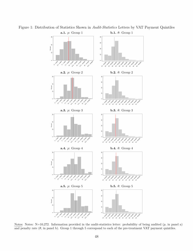
Figure 1: Distribution of Statistics Shown in Audit-Statistics Letters by VAT Payment Quintilesa.1. p: Group 1 b.1. θ: Group 1

010

2030

Per

cent

0 −

2.49

%

2.5

− 4.

99%

5 −

7.49

%

7.5

− 9.

99%

10 −

12.

49%

12.5

− 1

4.99

%

15 −

17.

49%

17.5

− 1

9.99

%

20 −

22.

49%

22.5

− 2

4.99

%

010

2030

40

15 −

19.

99%

20 −

24.

99%

25 −

29.

99%

30 −

34.

99%

35 −

39.

99%

40 −

44.

99%

45 −

49.

99%

50 −

54.

99%

55 −

59.

99%

60 −

64.

99%

65 −

69.

99%

a.2. p: Group 2 b.2. θ: Group 2

010

2030

Per

cent

0 −

2.49

%

2.5

− 4.

99%

5 −

7.49

%

7.5

− 9.

99%

10 −

12.

49%

12.5

− 1

4.99

%

15 −

17.

49%

17.5

− 1

9.99

%

20 −

22.

49%

22.5

− 2

4.99

%

010

2030

40

15 −

19.

99%

20 −

24.

99%

25 −

29.

99%

30 −

34.

99%

35 −

39.

99%

40 −

44.

99%

45 −

49.

99%

50 −

54.

99%

55 −

59.

99%

60 −

64.

99%

65 −

69.

99%

a.3. p: Group 3 b.3. θ: Group 3

010

2030

Per

cent

0 −

2.49

%

2.5

− 4.

99%

5 −

7.49

%

7.5

− 9.

99%

10 −

12.

49%

12.5

− 1

4.99

%

15 −

17.

49%

17.5

− 1

9.99

%

20 −

22.

49%

22.5

− 2

4.99

%

010

2030

40

15 −

19.

99%

20 −

24.

99%

25 −

29.

99%

30 −

34.

99%

35 −

39.

99%

40 −

44.

99%

45 −

49.

99%

50 −

54.

99%

55 −

59.

99%

60 −

64.

99%

65 −

69.

99%

a.4. p: Group 4 b.4. θ: Group 4

010

2030

Per

cent

0 −

2.49

%

2.5

− 4.

99%

5 −

7.49

%

7.5

− 9.

99%

10 −

12.

49%

12.5

− 1

4.99

%

15 −

17.

49%

17.5

− 1

9.99

%

20 −

22.

49%

22.5

− 2

4.99

%

010

2030

40

15 −

19.

99%

20 −

24.

99%

25 −

29.

99%

30 −

34.

99%

35 −

39.

99%

40 −

44.

99%

45 −

49.

99%

50 −

54.

99%

55 −

59.

99%

60 −

64.

99%

65 −

69.

99%

a.5. p: Group 5 b.5. θ: Group 5

010

2030

Per

cent

0 −

2.49

%

2.5

− 4.

99%

5 −

7.49

%

7.5

− 9.

99%

10 −

12.

49%

12.5

− 1

4.99

%

15 −

17.

49%

17.5

− 1

9.99

%

20 −

22.

49%

22.5

− 2

4.99

%

010

2030

40

15 −

19.

99%

20 −

24.

99%

25 −

29.

99%

30 −

34.

99%

35 −

39.

99%

40 −

44.

99%

45 −

49.

99%

50 −

54.

99%

55 −

59.

99%

60 −

64.

99%

65 −

69.

99%

Notes: Notes: N=10,272. Information provided in the audit-statistics letter: probability of being audited (p, in panel a)and penalty rate (θ, in panel b). Group 1 through 5 correspond to each of the pre-treatment VAT payment quintiles..

48

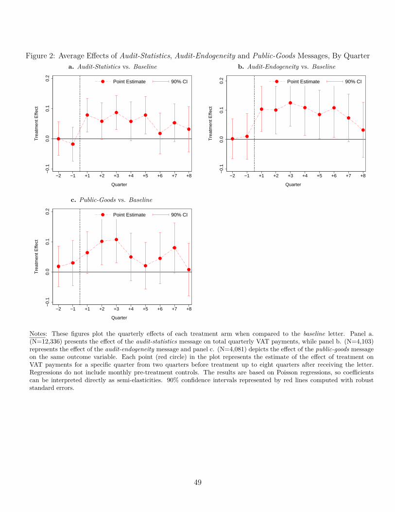
Figure 2: Average Effects of Audit-Statistics, Audit-Endogeneity and Public-Goods Messages, By Quartera. Audit-Statistics vs. Baseline b. Audit-Endogeneity vs. Baseline

−0.

10.

00.

10.

2

Tre

atm

ent E

ffect

−2 −1 +1 +2 +3 +4 +5 +6 +7 +8

Quarter

Point Estimate 90% CI

−0.

10.

00.

10.

2

Tre

atm

ent E

ffect

−2 −1 +1 +2 +3 +4 +5 +6 +7 +8

Quarter

Point Estimate 90% CI

c. Public-Goods vs. Baseline

−0.

10.

00.

10.

2

Tre

atm

ent E

ffect

−2 −1 +1 +2 +3 +4 +5 +6 +7 +8

Quarter

Point Estimate 90% CI

Notes: These figures plot the quarterly effects of each treatment arm when compared to the baseline letter. Panel a.(N=12,336) presents the effect of the audit-statistics message on total quarterly VAT payments, while panel b. (N=4,103)represents the effect of the audit-endogeneity message and panel c. (N=4,081) depicts the effect of the public-goods messageon the same outcome variable. Each point (red circle) in the plot represents the estimate of the effect of treatment onVAT payments for a specific quarter from two quarters before treatment up to eight quarters after receiving the letter.Regressions do not include monthly pre-treatment controls. The results are based on Poisson regressions, so coefficientscan be interpreted directly as semi-elasticities. 90% confidence intervals represented by red lines computed with robuststandard errors..

49

Figure 3: Survey Results: Perception of Audit Probabilities and of Tax Evasion Penalty Rates by Treat-ment Group

Audit Probability (p) Penalty Rate (θ)a. Audit-Statistics vs. Baseline and Public-Goods b. Audit-Statistics vs. Baseline and Public-Goods

Letters

010

2030

4050

60P

erce

nt

0 −

9.99

%

10 −

19.

99%

20 −

29.

99%

30 −

39.

99%

40 −

49.

99%

50 −

59.

99%

60 −

69.

99%

70 −

79.

99%

80 −

89.

99%

90 −

100

%

Audit Probability (%)

Perceived (pooled control group)Mean = 40.7%Perceived (audit−statistics)Mean = 35.2%Diff − p−value: 0.03

Letters

010

2030

40P

erce

nt

0 −

9.99

%

10 −

19.

99%

20 −

29.

99%

30 −

39.

99%

40 −

49.

99%

50 −

59.

99%

60 −

69.

99%

70 −

79.

99%

80 −

89.

99%

90%

+

Penalty Size (%)

Perceived (pooled control group)Mean = 30.5%Perceived (audit−statistics)Mean = 29.9%Diff − p−value: 0.85

Notes: The histograms are based on survey responses from those who reported themselves as owners in the post-treatmentsurvey. Perceived (pooled control group, N=137) refers to to survey respondents who received the baseline (N=69) orthe public-goods (N=68) letters during the experimental stage (none of the two letters contained any information aboutaudit probabilities nor penalty rates). Perceived (aud.–statistics) refers to respondents who received audit-statistics letters(N=365). In panel a. the x-axis represents the probability of being audited; in panel b. it represents the average penaltyrate. We report the mean responses and the p-value of the difference between the two groups. The answers correspond toquestions Q2 and Q4 (see full survey questionnaire in Appendix A.7). The red line represents the density function of theinformation displayed in the audit-statistics letters, measured in the right y-axis (hidden for the sake clarity)..

50

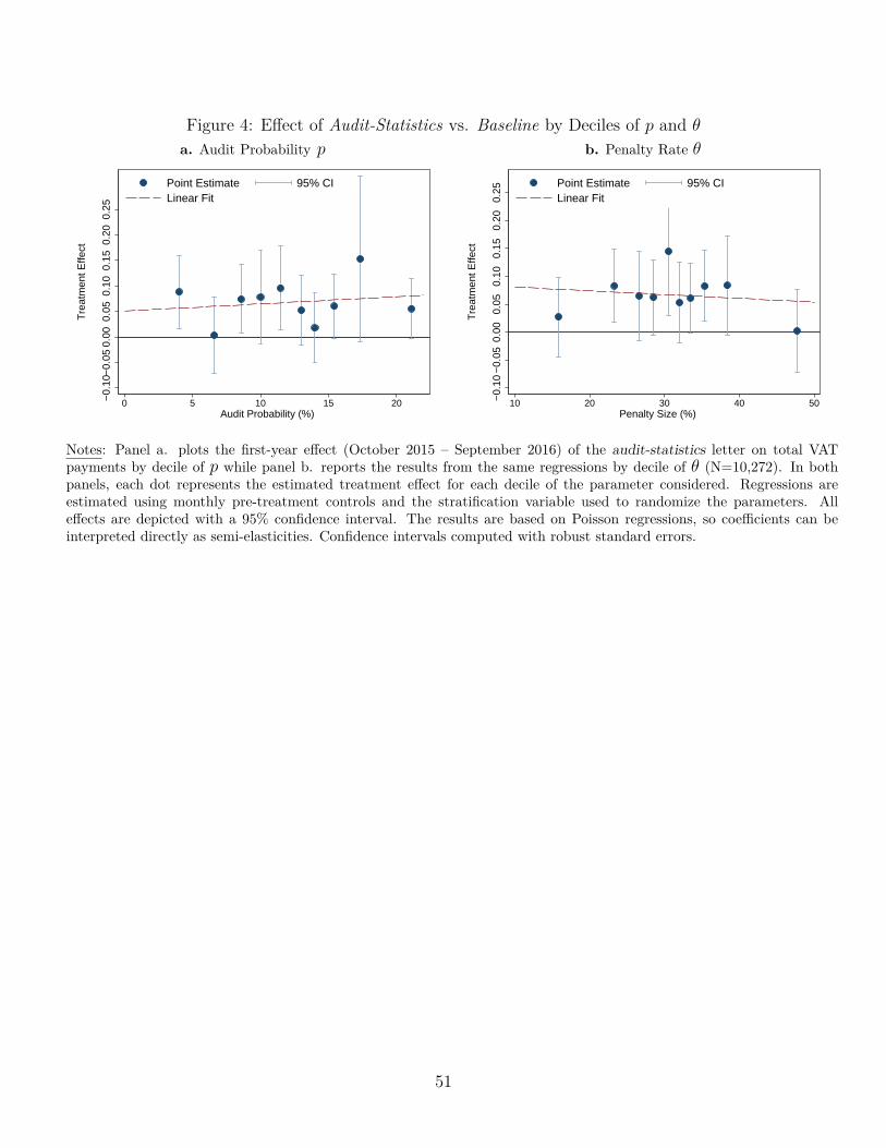
Figure 4: Effect of Audit-Statistics vs. Baseline by Deciles of p and θa. Audit Probability p b. Penalty Rate θ

−0.

10−

0.05

0.00

0.05

0.10

0.15

0.20

0.25

Tre

atm

ent E

ffect

0 5 10 15 20Audit Probability (%)

Point Estimate 95% CILinear Fit

−0.

10−

0.05

0.00

0.05

0.10

0.15

0.20

0.25

Tre

atm

ent E

ffect

10 20 30 40 50Penalty Size (%)

Point Estimate 95% CILinear Fit

Notes: Panel a. plots the first-year effect (October 2015 – September 2016) of the audit-statistics letter on total VATpayments by decile of p while panel b. reports the results from the same regressions by decile of θ (N=10,272). In bothpanels, each dot represents the estimated treatment effect for each decile of the parameter considered. Regressions areestimated using monthly pre-treatment controls and the stratification variable used to randomize the parameters. Alleffects are depicted with a 95% confidence interval. The results are based on Poisson regressions, so coefficients can beinterpreted directly as semi-elasticities. Confidence intervals computed with robust standard errors..

51

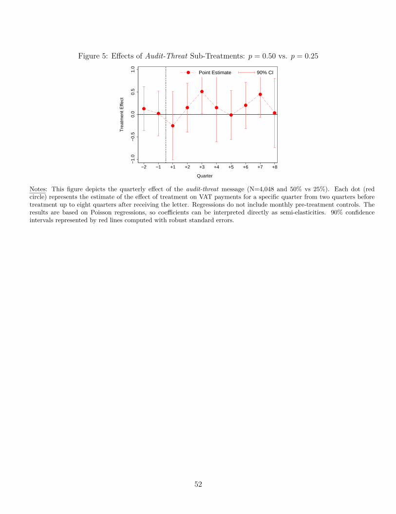
Figure 5: Effects of Audit-Threat Sub-Treatments: p = 0.50 vs. p = 0.25

−1.

0−

0.5

0.0

0.5

1.0

Tre

atm

ent E

ffect

−2 −1 +1 +2 +3 +4 +5 +6 +7 +8

Quarter

Point Estimate 90% CI

Notes: This figure depicts the quarterly effect of the audit-threat message (N=4,048 and 50% vs 25%). Each dot (redcircle) represents the estimate of the effect of treatment on VAT payments for a specific quarter from two quarters beforetreatment up to eight quarters after receiving the letter. Regressions do not include monthly pre-treatment controls. Theresults are based on Poisson regressions, so coefficients can be interpreted directly as semi-elasticities. 90% confidenceintervals represented by red lines computed with robust standard errors..

52

Figure 6: Effect of Audit-Statistics vs. Baseline by Prior Beliefsa. Audit probability - prior (calibrated to 11.7%) b. Audit probability - prior - signal (calibrated to 11.7%)

−0.

10−

0.05

0.00

0.05

0.10

0.15

0.20

0.25

Tre

atm

ent E

ffect

0 10 20 30 40 50 60 70Prior Belief: Audit Probability (%)

Point Estimate95% CILinear Fit

−0.

10−

0.05

0.00

0.05

0.10

0.15

0.20

0.25

Tre

atm

ent E

ffect

0 10 20 30 40 50 60Prior Belief: Audit Probability (%)

Point Estimate95% CILinear Fit

Notes: Panel a. plots the first-year effect (October 2015 – September 2016) of the audit-statistics letter on total VATpayments by quartiles of prior beliefs while panel b. reports the same results by quartiles of the difference between the priorbelief and the signal sent in the audit-statistics message (N=11,989). The prior belief (before the experiment) is computedas p̂i = 1−

(1− α0+Ni

α0+β0+Ti

)3

such that the mean prior belief about the probability of being audited at least once in the following three years matchesthe actual average probability observed in our sample. In panel b. the signal for the placebo group was randomly assignedusing the same strategy that for the audit-statistics group. The red dashed line represents the linear fit corresponding tothe four estimates . In panel a., the dashed green line represents the average perceived probability (11.7%). In panel b.,the dashed green line represents the point in which prior belief and signal are equal. In both panels, each dot representsthe estimated treatment effect for each quartile of the variable considered. Regressions are estimated using monthly pre-treatment controls. All effects are depicted with 95% confidence interval. The results are based on Poisson regressions, socoefficients can be interpreted directly as semi-elasticities. Confidence intervals are computed with robust standard errors..

53

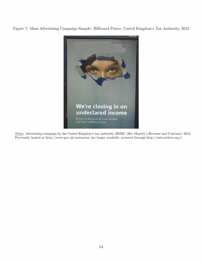
Figure 7: Mass Advertising Campaign Sample: Billboard Poster, United Kingdom’s Tax Authority, 2012

Notes: Advertising campaign by the United Kingdom’s tax authority, HMRC (Her Majesty’s Revenue and Customs), 2012.Previously hosted at http://www.gov.uk/sortmytax (no longer available, accessed through http://web.archive.org/).

54

Online Appendix: For Online Publication Only

A Replication Material: Letters and Survey

This appendix presents samples of the five types of letter in our experiment: the baseline letter (A.1),the audit-statistics letter (A.2), the audit-threat letter (A.3), the audit-endogeneity letter (A.4) and thepublic goods letter (A.5). Additionally, Appendix A.6 presents a sample of the invitation sent by emailby the IRS to complete the online survey, and Appendix A.7 presents the questionnaire module aboutperceptions of audit probabilities and penalty rates that we designed and that was included in the survey.

i

A.1 Sample Letter: Baseline Letter

Montevideo, August 20th 2015 Mr../Ms. Taxpayer: The DGI has the authority to perform inspections (see Art. 68 of the tax code) and routine audits of taxpayers on the basis of crosschecks and assessment of data compiled to detect oversights and inconsistency on tax returns as well as pending tax debts. The aim of the DGI, and the primary challenge it faces, is to ensure the collection of revenue to sustain life in society. Additionally, its task is to generate a framework of fair and transparent competition where the failure of some to meet their obligations does not have an unfavorable impact on honest taxpayers. In order to meet these goals, inspections are performed in a routine fashion. Your micro, small, or medium-sized business has been randomly selected to receive this information. It is solely for your information and its receipt does not require you to present any documentation to the DGI offices. We ask you to comply with your tax obligations for the sake of the country we all want, a more and more developed Uruguay with greater and greater social cohesion. Sincerely,

Collection and Controls Division

Internal Revenues Services

ii

A.2 Sample Letter: Audit-Statistics Letter

Montevideo, August 20th 2015 Mr../Ms. Taxpayer: The DGI has the authority to perform inspections (see Art. 68 of the tax code) and routine audits of taxpayers on the basis of crosschecks and assessment of data compiled to detect oversights and inconsistency on tax returns as well as pending tax debts.

On the basis of historical information on similar businesses, there is a probability of p% that the tax returns you filed for this year will be audited in at least one of the coming three years. If, pursuant to that auditing, it is determined that tax evasion has occurred, you will be required to pay not only the amount previously unpaid, but also a fee of

approximately 𝜽% of that amount.

The aim of the DGI, and the primary challenge it faces, is to ensure the collection of revenue to sustain life in society. Additionally, its task is to generate a framework of fair and transparent competition where the failure of some to meet their obligations does not have an unfavorable impact on honest taxpayers. In order to meet these goals, inspections are performed in a routine fashion. Your micro, small, or medium-sized business has been randomly selected to receive this information. It is solely for your information and its receipt does not require you to present any documentation to the DGI offices. We ask you to comply with your tax obligations for the sake of the country we all want, a more and more developed Uruguay with greater and greater social cohesion. Sincerely,

Collection and Controls Division

Internal Revenues Services

iii

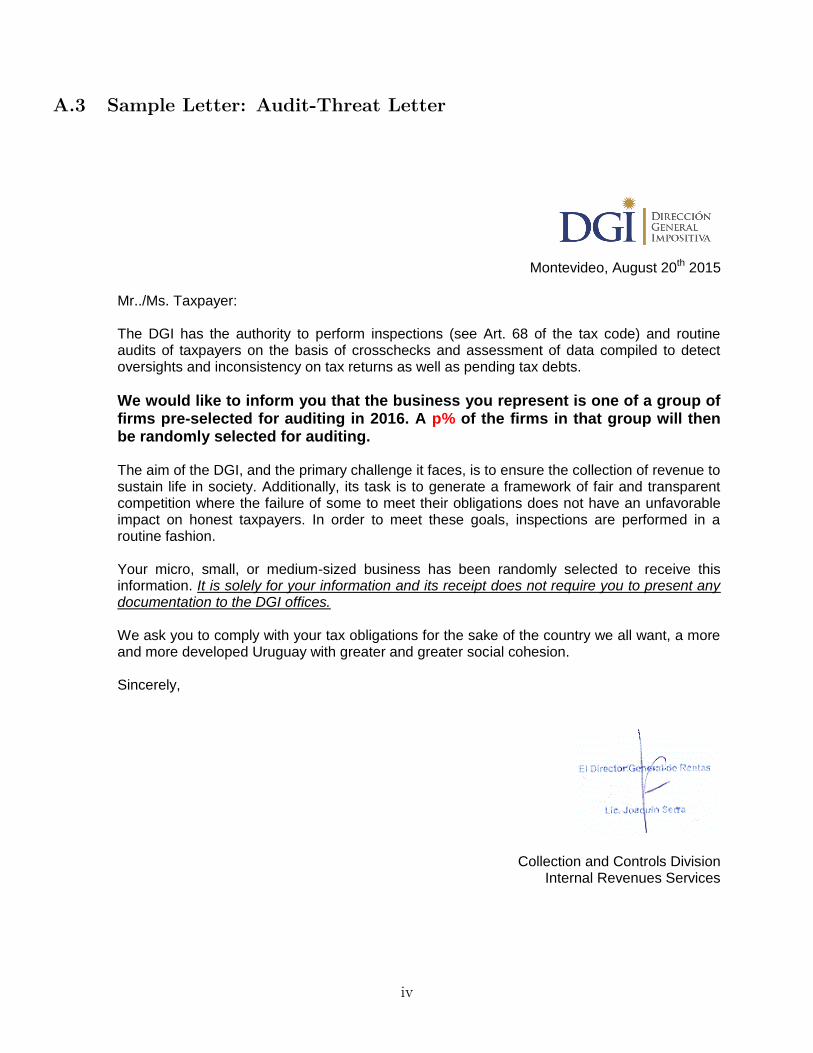
A.3 Sample Letter: Audit-Threat Letter

Montevideo, August 20th 2015 Mr../Ms. Taxpayer: The DGI has the authority to perform inspections (see Art. 68 of the tax code) and routine audits of taxpayers on the basis of crosschecks and assessment of data compiled to detect oversights and inconsistency on tax returns as well as pending tax debts.

We would like to inform you that the business you represent is one of a group of firms pre-selected for auditing in 2016. A p% of the firms in that group will then be randomly selected for auditing. The aim of the DGI, and the primary challenge it faces, is to ensure the collection of revenue to sustain life in society. Additionally, its task is to generate a framework of fair and transparent competition where the failure of some to meet their obligations does not have an unfavorable impact on honest taxpayers. In order to meet these goals, inspections are performed in a routine fashion. Your micro, small, or medium-sized business has been randomly selected to receive this information. It is solely for your information and its receipt does not require you to present any documentation to the DGI offices. We ask you to comply with your tax obligations for the sake of the country we all want, a more and more developed Uruguay with greater and greater social cohesion. Sincerely,

Collection and Controls Division Internal Revenues Services

iv

A.4 Sample Letter: Audit-Endogeneity Letter

Montevideo, August 20th 2015 Mr../Ms. Taxpayer: The DGI has the authority to perform inspections (see Art. 68 of the tax code) and routine audits of taxpayers on the basis of crosschecks and assessment of data compiled to detect oversights and inconsistency on tax returns as well as pending tax debts.

The DGI uses data on thousands of taxpayers to detect firms that may be evading taxes; most of its audits are aimed at those firms. Evading taxes, then, doubles your chances of being audited. The aim of the DGI, and the primary challenge it faces, is to ensure the collection of revenue to sustain life in society. Additionally, its task is to generate a framework of fair and transparent competition where the failure of some to meet their obligations does not have an unfavorable impact on honest taxpayers. In order to meet these goals, inspections are performed in a routine fashion. Your micro, small, or medium-sized business has been randomly selected to receive this information. It is solely for your information and its receipt does not require you to present any documentation to the DGI offices. We ask you to comply with your tax obligations for the sake of the country we all want, a more and more developed Uruguay with greater and greater social cohesion. Sincerely,

Collection and Controls Division

Internal Revenues Services

v

A.5 Sample Letter: Public-Goods Letter

Montevideo, August 20th 2015 Mr../Ms. Taxpayer: The DGI has the authority to perform inspections (see Art. 68 of the tax code) and routine audits of taxpayers on the basis of crosschecks and assessment of data compiled to detect oversights and inconsistency on tax returns as well as pending tax debts.

If those who currently evade their tax obligations were evade 10% less, the additional revenue collected would enable all of the following: to supply 42,000 portable computers to school children; to build 4 high schools, 9 elementary schools, and 2 technical schools; to acquire 80 patrol cars and to hire 500 police officers; to add 87,000 hours of medical attention by doctors at public hospitals; to hire 660 teachers; to build 1,000 public housing units (50m2 per unit). There would be resources left over to reduce the fiscal burden. The tax behavior of each of us has direct effects on the lives of us all. The aim of the DGI, and the primary challenge it faces, is to ensure the collection of revenue to sustain life in society. Additionally, its task is to generate a framework of fair and transparent competition where the failure of some to meet their obligations does not have an unfavorable impact on honest taxpayers. In order to meet these goals, inspections are performed in a routine fashion. Your micro, small, or medium-sized business has been randomly selected to receive this information. It is solely for your information and its receipt does not require you to present any documentation to the DGI offices. We ask you to comply with your tax obligations for the sake of the country we all want, a more and more developed Uruguay with greater and greater social cohesion. Sincerely,

Collection and Controls Division

Internal Revenues Services

vi

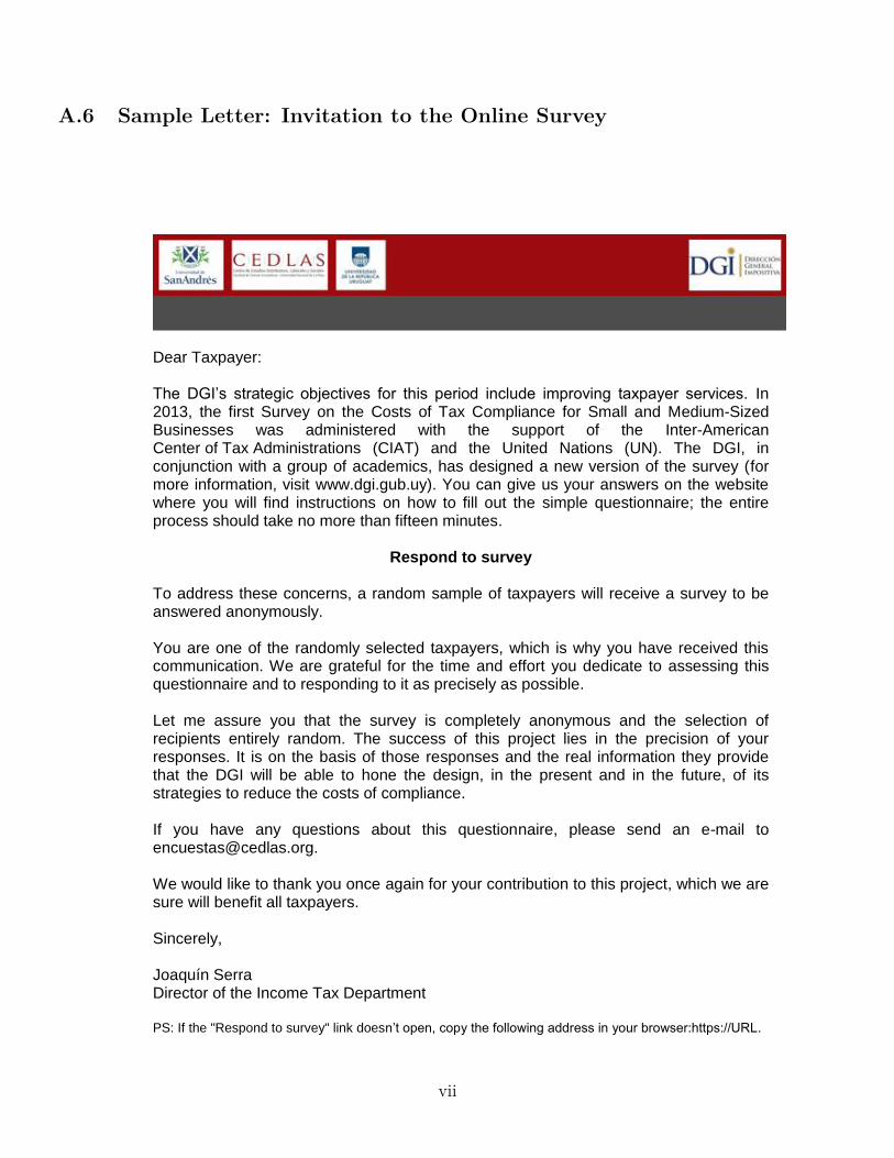
A.6 Sample Letter: Invitation to the Online Survey

Dear Taxpayer: The DGI’s strategic objectives for this period include improving taxpayer services. In 2013, the first Survey on the Costs of Tax Compliance for Small and Medium-Sized Businesses was administered with the support of the Inter-American Center of Tax Administrations (CIAT) and the United Nations (UN). The DGI, in conjunction with a group of academics, has designed a new version of the survey (for more information, visit www.dgi.gub.uy). You can give us your answers on the website where you will find instructions on how to fill out the simple questionnaire; the entire process should take no more than fifteen minutes.

Respond to survey To address these concerns, a random sample of taxpayers will receive a survey to be answered anonymously. You are one of the randomly selected taxpayers, which is why you have received this communication. We are grateful for the time and effort you dedicate to assessing this questionnaire and to responding to it as precisely as possible. Let me assure you that the survey is completely anonymous and the selection of recipients entirely random. The success of this project lies in the precision of your responses. It is on the basis of those responses and the real information they provide that the DGI will be able to hone the design, in the present and in the future, of its strategies to reduce the costs of compliance. If you have any questions about this questionnaire, please send an e-mail to encuestas@cedlas.org. We would like to thank you once again for your contribution to this project, which we are sure will benefit all taxpayers. Sincerely, Joaquín Serra Director of the Income Tax Department PS: If the "Respond to survey" link doesn’t open, copy the following address in your browser:https://URL.

vii

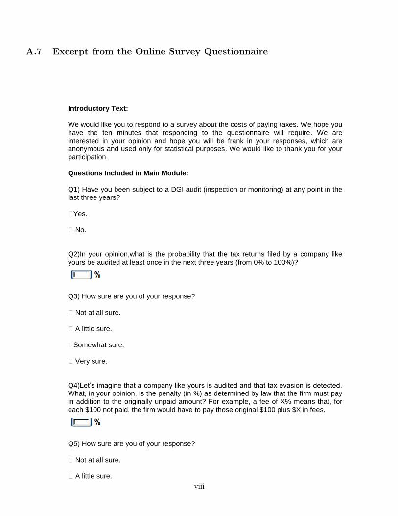
A.7 Excerpt from the Online Survey Questionnaire

Introductory Text: We would like you to respond to a survey about the costs of paying taxes. We hope you have the ten minutes that responding to the questionnaire will require. We are interested in your opinion and hope you will be frank in your responses, which are anonymous and used only for statistical purposes. We would like to thank you for your participation. Questions Included in Main Module: Q1) Have you been subject to a DGI audit (inspection or monitoring) at any point in the last three years? Yes. No. Q2)In your opinion,what is the probability that the tax returns filed by a company like yours be audited at least once in the next three years (from 0% to 100%)?

Q3) How sure are you of your response? Not at all sure. A little sure. Somewhat sure. Very sure. Q4)Let’s imagine that a company like yours is audited and that tax evasion is detected. What, in your opinion, is the penalty (in %) as determined by law that the firm must pay in addition to the originally unpaid amount? For example, a fee of X% means that, for each $100 not paid, the firm would have to pay those original $100 plus $X in fees.

Q5) How sure are you of your response? Not at all sure. A little sure.

viii

B Additional Results, Specifications and Robustness Checks

B.1 Summary Statistics of Tax Payments

Table B.1 describes the tax payments made by firms that received the baseline letter during the preand post treatment period. The pre-treatment period covers the year immediately before the treatment(September 2014 – August 2015) and analogously the post-treatment period covers the twelve immediatemonths after the treatment (October 2015 – September 2016). On average, the amount of VAT paid bya firm that received a baseline letter during the pre-treatment period was USD 7,770 while the medianwas around USD 4,860, with a standard deviation of USD 8,070. In the subsequent year, the averageamount of VAT paid was USD 6,470, the median USD 7,770 and the standard deviation USD 3,740. Thisrepresents a reduction of 16,7% in the average VAT payments when comparing post and pre-treatmentperiods. Since the group of firms we analyze are mainly small and medium sized firms, this could beexplained by a high turnover rate.

Retroactive VAT payments made by the firms show that most of taxpayers do not made this typeof payments. Indeed, the 75th percentile of this distribution is 0. The average amount of backwardpayments made by these firms during the pre-treatment period was USD 400, while during the posttreatment period it was about 300 USD. This is consistent with the trend observed for overall VATpayments. This is also confirmed when considering payments of other taxes. On average, firms paid USD4,070 of other taxes in the pre-treatment period, and USD 3,300 in the post-treatment period. Theseamounts correspond to other taxes applied to retail sales of specific goods and corporate taxes, amongothers. The standard deviation in the pre-treatment distribution was USD 8,570 in the pre-treatmentperiod, which fell to USD 5,430 in the post treatment period.

This descriptive analysis is indicative of the importance of the VAT in the Uruguayan tax structure.VAT payments are almost twice as much as payments of other taxes payments, and they represent morethan 60% of the total payments by firms in our sample.

B.2 Robustness Checks: Regression Analysis

B.2.1 Robustness Checks of Main Specification

To assess the robustness of the results from the main specification in Section 4, Table B.2 presentsalternative estimates based on different specifications. The first two columns present estimates of thetreatment effects based only on the extensive margin of VAT payments: i.e., the outcome is coded as1 if the firm made at least one payment in the post-treatment period, and 0 otherwise. Column (1)presents results from a linear probability model, while column (2) presents Probit estimates. There isnot much variation in the extensive margin: 96% of firms in the sample made positive payments in thepost-treatment period. This is a direct byproduct of the selection of the subject pool: we excluded all

ix

firms who did not make at least three payments in the 12 months before the treatment assignment. Theeffects of the three different messages on the extensive margin are close to zero and not statisticallysignificant, although the precision of our estimates does not allows to reject a large effect in the extensivemargin.

The specifications in columns (3), (4) and (5) of Table B.2 use the amount of VAT payments as thedependent variable. Column (3) corresponds to our main Poisson specification. In turn, column (4)presents estimates based on Tobit regressions and (5) presents OLS estimates. The Poisson model hasa main advantage in this context: it deals naturally with bunching of payments at exactly zero, whilestill allowing for the effects to be proportional. The OLS specification, instead, does not deal with thebunching at zero and does not allow for the effects on amounts to be proportional. The Tobit specificationis more appropriate than OLS since it takes into account the censored nature of the data at zero, but itdoes not allow for the effects to be proportional.

The results from columns (3), (4) and (5) of Table B.2 are identical in terms of the signs and statisticalsignificance of the coefficients, indicating that the results are robust to the three alternative specifications.If anything, the effects are more statistically significant when using the OLS and Tobit models. Eventhough the results from the Poisson, OLS and Tobit models are not directly comparable in terms ofmagnitudes, they are roughly consistent. For example, the Tobit model suggests an effect of audit-statistics of USD 480 (p-value=0.001). Since the average outcome is USD 6,465, this Tobit coefficientamounts to an effect of about 7.4%, which is in the same order of magnitude than the Poisson model,which indicates an effect of audit-statistics of 6.3% (p-value=0.013).

Column (6) of Table B.2 reports the results of estimating our model on the final tax liability calculatedon data from an alternative administrative data source, annual tax returns. The time frame in thisoutcome is completely different to the one of the monthly VAT payments used for our main specification,and therefore they do not necessarily match. However, the results in column (6), panel a in Table B.2indicate that the effect of the audit-statistic letter is 6.8% with this alternative measure of the outcomevariable, which is indeed similar in sign and magnitude to our main result. This effect is estimatedprecisely and statistical significant at the 5% level. The effect of the treatment in the falsification test isindistinguishable from zero.

The results in panel b in Table B.2 indicate shows that the effect of the endogeneity message on theVAT reported in the annual tax return is also similar to the effect on the monthly VAT payments. Thepoint estimate of the coefficient is 5.6%, smaller than the result for our main specification. However,in this case the coefficient is less precisely estimated, and it is not statistically different from zero atconventional levels. Finally, the results in panel c in Table B.2 indicate that the effect of the public-goodsletter on the VAT liability reported in the tax return is also close to zero, as in our main results.

x

B.2.2 Robustness Checks for Heterogeneity With Respect to Prior Beliefs and PreviousAudit Experience

As an additional robustness check for heterogeneous results in terms of prior beliefs, we present the effectof the treatment by whether the firms’ prior belief p̂ (as defined in section B.2) was below or above thespecific value of p in the letter sent to the firm as part of the audit-statistics treatment (the distribution ofthe parameters included in our audit-statistics letters is depicted in Figure 1). To estimate this effect, wedivided the sample in two groups. On the one hand, firms with prior beliefs about the probability of beingaudited that were low compared to the probability reported in the letter they received. On the otherhand, firms with prior beliefs equal or larger than the parameter reported in our information treatment.Since we divide the groups according to a characteristic of firms that received the audit-statistics message,the outcomes for both groups are compared to those of the firms that received the baseline letter.

According to the A&S model, increasing taxpayers’ beliefs about the probability of being auditedshould result in higher tax payments (the opposite is also true if we reduce their perception about p).Therefore, the expected effect of the audit-statistics message is positive on firms with p̂ < p, and negativefor firms with p̂ ≥ p. Column (2) in Table B.3 shows that the average effect of the audit-statistics letteron VAT payments in the first year after receiving the letter is 7.1% for taxpayers with relatively lowpriors. Column (3) reports that the average effect for taxpayers with relatively large priors was 9.1%.The effect in firms with relatively low priors is positive but lower in magnitude compared to firms withrelatively high priors, and the effect on the latter has the opposite sign of the one predicted by the model.Furthermore, differences in magnitude are economically not significant. These results, if anything, provideevidence against the A&S predictions.

We can also test whether actual audit experience has an effect on our treatments. In columns (3)and (4) in Table B.3, we compare the effects of the audit-statistics message between firms that wereaudited in the recent past (up to 15 years before the treatment, 23,8% of the sample) and those thatwere not audited during that period (the remaining 76,2% of the sample). We use the previous 15years because that is how far back the available IRS administrative records reach. The intuition is thatfirms that were audited in the recent past should have a higher perception of the probability of beingaudited. The null hypothesis thus is that the effect of our audit-statistics messages should be strongerfor those that were never audited, who probably had priors about audit probabilities closer to zero andincreased their perceived probability with our messages. Moreover, we could even expect negative effectson compliance for those who were audited in the past, because these firms probably had high priors aboutaudit probabilities and our information treatment should have reduced their perceptions. The results inTable B.3 indicate that there are no heterogeneous effects with respect to recent audit experience. Thedifference in treatment effects for the two groups is small and not statistically significant: the effect is4.7% for the group of firms previously audited, and 7.1% for those with no prior audit experience (p-valueof difference = 0.252). However, the number of firms that were audited is smaller (N=2,933) than that of

xi

firms that were not audited in the recent past (N=9,403), and thus the coefficients for the former groupare less precisely estimated. As a result, we cannot rule out moderate differences either between the twogroups.

We can also perform a further robustness check of our Bayesian model. For our third test, we mustset the parameters α0 and β0 to generate the prior beliefs. In the body of the paper, we selected valuesof these parameters to “center” beliefs around the true audit probability in our sample, 11.7%. Sincethis choice may seem arbitrary, we present the results from an alternative calibration, which centers theperceived probability around the value we obtain from the control group in our post-treatment survey –an average perceived audit probability of 40.5% for the comparison group. The results are presented inFigure B.2. If anything, this alternative calibration makes A&S even less plausible: as shown in panelb, we would expect that almost everyone should update their perceived probability downwards, and thusreduce their tax payments, which is the opposite of what we find.

B.2.3 Alternative Specifications for the Effects of Signals about Audit Probabilities andPenalty Rates

We also assess the robustness of the estimated effects of the signals of audit probabilities and penaltyrates on post-treatment payments in two different ways.

First, Table B.4 a. replicates the analysis in Table 4 for the five additional specifications that wealso used in Table B.2. The results are essentially the same that the ones reported in section 5. Theeffect of the information provided within firms that received the audit-statistics letter is zero. Both inthe extensive and intensive margin, regardless of the specification used or the source of the dependentvariable (using the tax liability from the annual tax returns as an outcome), all coefficients associated tothe treatment variable are statistically insignificant. This is also valid for the effects of the audit-threatmessage. Conditional on being treated, the information reported in the letter does not affect firms’compliance behavior.

Second, Table B.5 presents the results for an alternative specification of the elasticity estimation inTable 4. Instead of estimating the elasticities with respect to p and θ separately, we estimate the elasticitywith respect to the product (expected penalty) p ∗ θ in a regression of the form:

Yi = α + γp·θ · pi · θi +Xiδ + εi (B.1)

As in the model where p and θ were included separately, the elasticity computed with this alternativespecification is statistically and economically insignificant.

Figure B.3.a provides additional an event-study analysis of the effect of the audit-statistics message(relative to the baseline letter) for two groups: firms that received letters with low signals of p (p<=11.7%)and those who received high signals of p (p>11.7%). The estimates in these figures are obtained from

xii

regressions that control for the group dummies (quintiles of VAT payments), so they are identified purelyby the random sampling variation in p. Note that the effects are extremely similar for the two groups.If anything, the treatment effects seem larger for the group with the lower probability messages. FigureB.3.b presents the equivalent analysis for firms that received messages with low and high values of θ(below and above the mean penalty rate in our sample, 30.6%). Again, the effects are very similar forthe two groups.

The results in Tables B.2 and B.5, and Figure B.3, provide further evidence supporting the fearchannel rather than a rational re optimization as a consequence of being exposed to some informationabout the tax enforcement mechanisms.

B.3 Robustness Checks and Additional Results from Online Survey

B.3.1 Survey Results: Robustness to the Control Group Definition

Our analysis of the survey relied on pooling respondents from the baseline and the public-goods to forma sufficiently large comparison group. The rationale was that neither of the two messages includedinformation about audit probabilities or tax evasion penalty rates. In this appendix, we assess therobustness of the survey results in section 5.1 to alternative definitions of the sample and of the comparisongroup.

Panels a and b in Figure B.3 replicates the results in panels a and b in Figure 3. The shaded graybars show the distribution of perceptions for the 69 survey respondents that received the baseline letteronly (Figure 3 relied on the 137 observations from the pooled baseline and public-goods groups). Thered dashed curve correspond to the distribution of signals sent to the firms in the audit-statistics letters.Although slightly smaller than in the pooled control group, the average perceived audit probability ofthe baseline letter group (37.7%) is still substantially larger than the 11.7% that results from our data forthe overall sample, and this difference is statistically significant. The results are also consistent with themain results when we look at the perceived penalty size. There are no statistically significant differencesbetween the perceived penalty size by the firms that received the baseline letter and our estimates fromthe overall data.

We also replicate the analysis the average effect of the audit-statistic message on the perceived auditprobability and penalty size. The average perceived probability of being audited for the baseline groupis 37.7%, which is slightly smaller than the one reported by the pooled control group (40.7%). Since thisnumber is closer to the average perceived audit probability for the audit-statistics group (35.2%) and thestatistical power is substantially reduced by the lower number of observations (the control group reducedto the half), the mean difference test does not reject the null that both means are equal. However, theresults are in the same direction that our main results. If anything, the audit-statistics letter reducedthe average perceived probability of being audited. The results of the penalty size differences between

xiii

treated and control groups are also consistent with the main results. The audit-statistics letter did notaffect taxpayers perceptions about the average penalty size and in general the prior beliefs of the firmswere accurate.

Finally, we present an additional robustness test of the results in Figure 3. To increase the likelihoodthat survey respondents were the ones who received our experimental messages, we impose an additionalrestriction. We do the same analysis but restricting our sample to survey respondents who self-identifiedas firm owners in the survey. The results with this restricted sample (which reduced the treatment groupfrom 365 to 341 observations, and the pooled control group from 137 to 125), presented in panels c and din Figure B.3, are very similar to those reported in the body of the paper. Our audits-statistics treatmentsignificantly reduced the perceived probability of audits, although it did not affect the average perceptionof penalty rates.

If firms were rational, all these results would imply that firms would have paid less taxes as a con-sequence of the update in their beliefs. However, this is not what it is observed. Hence, this evidencesupports the hypothesis that the fear channel is driving the results rather than a rational re-optimization.

B.3.2 Beliefs About Audit Endogeneity

As in the case of the audit-statistics treatment arm, we conducted a survey of letter recipients in whichwe included a specific question to assess whether the information provided in the letter had an impacton beliefs about the endogeneity of audits:

Perceived Audit Endogeneity: “In your opinion, if a firm that evades taxes doubles the amountit is evading, what is the effect on its probability of being audited?” The possible answerswere: It would increase significantly; It would increase slightly; It would not change; It woulddiminish slightly; It would diminish significantly.

The distribution of responses to this question about the perceived endogeneity of audits is depicted inFigure B.5. The distribution of perceptions in the baseline letter suggests that firms were already awareof this endogeneity. Relative to the baseline group, there are no statistically significant differences inthe distribution of perceptions for the audit-endogeneity group. In a scale from 1 to 5, where 1 is “moreevasion significantly increases the probability of being audited”, and 5 means “more evasion significantlydiminish the probability of being audited”, the average belief was 1.45 in the baseline group and 1.41 forthe audit-endogeneity group (p-value of the difference 0.67).

xiv

Table B.1: Tax Payments: Summary StatisticsMean(1)

SD(2)

10th(3)

25th(4)

50th(5)

75th(6)

90th(7)

VAT AmountsPost-treatment 6.47 7.77 0.44 1.30 3.74 8.48 16.55Pre-Treatment 7.77 8.07 0.96 1.99 4.86 10.94 19.73

Retroactive VAT AmountsPost-treatment 0.30 1.40 0.00 0.00 0.00 0.00 0.62Pre-Treatment 0.40 1.76 0.00 0.00 0.00 0.00 0.81

Other Taxes AmountsPost-Treatment 3.30 5.43 0.00 0.95 1.81 3.52 7.42Pre-Treatment 4.07 8.57 0.04 1.43 2.14 4.37 8.72

Notes: The statistics in this table correspond to firms that received the baseline letter (N=2,064). The pre-treatmentperiod ranges from September 1, 2014 to August 31, 2015, and the post-treatment period ranges from October 1, 2015to September 30, 2016. The source of the data are IRS administrative data records. VAT amounts corresponds to VATpayments and withholdings. Retroactive VAT amounts correspond to two months or more retroactive VAT payments andwithholdings, e.g. VAT payments made in March 2016 corresponding to September 2015. Other taxes includes paymentsfor the corporate tax, the wealth tax and other specific taxes to business activity..

xv

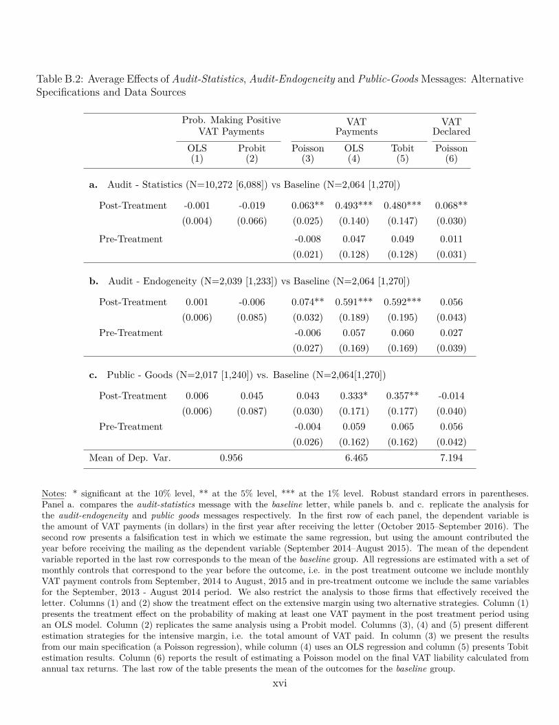
Table B.2: Average Effects of Audit-Statistics, Audit-Endogeneity and Public-Goods Messages: AlternativeSpecifications and Data Sources

Prob. Making PositiveVAT Payments

VATPayments

VATDeclared

OLS(1)

Probit(2)

Poisson(3)

OLS(4)

Tobit(5)

Poisson(6)

a. Audit - Statistics (N=10,272 [6,088]) vs Baseline (N=2,064 [1,270])

Post-Treatment -0.001 -0.019 0.063** 0.493*** 0.480*** 0.068**(0.004) (0.066) (0.025) (0.140) (0.147) (0.030)

Pre-Treatment -0.008 0.047 0.049 0.011(0.021) (0.128) (0.128) (0.031)

b. Audit - Endogeneity (N=2,039 [1,233]) vs Baseline (N=2,064 [1,270])

Post-Treatment 0.001 -0.006 0.074** 0.591*** 0.592*** 0.056(0.006) (0.085) (0.032) (0.189) (0.195) (0.043)

Pre-Treatment -0.006 0.057 0.060 0.027(0.027) (0.169) (0.169) (0.039)

c. Public - Goods (N=2,017 [1,240]) vs. Baseline (N=2,064[1,270])

Post-Treatment 0.006 0.045 0.043 0.333* 0.357** -0.014(0.006) (0.087) (0.030) (0.171) (0.177) (0.040)

Pre-Treatment -0.004 0.059 0.065 0.056(0.026) (0.162) (0.162) (0.042)

Mean of Dep. Var. 0.956 6.465 7.194

Notes: * significant at the 10% level, ** at the 5% level, *** at the 1% level. Robust standard errors in parentheses.Panel a. compares the audit-statistics message with the baseline letter, while panels b. and c. replicate the analysis forthe audit-endogeneity and public goods messages respectively. In the first row of each panel, the dependent variable isthe amount of VAT payments (in dollars) in the first year after receiving the letter (October 2015–September 2016). Thesecond row presents a falsification test in which we estimate the same regression, but using the amount contributed theyear before receiving the mailing as the dependent variable (September 2014–August 2015). The mean of the dependentvariable reported in the last row corresponds to the mean of the baseline group. All regressions are estimated with a set ofmonthly controls that correspond to the year before the outcome, i.e. in the post treatment outcome we include monthlyVAT payment controls from September, 2014 to August, 2015 and in pre-treatment outcome we include the same variablesfor the September, 2013 - August 2014 period. We also restrict the analysis to those firms that effectively received theletter. Columns (1) and (2) show the treatment effect on the extensive margin using two alternative strategies. Column (1)presents the treatment effect on the probability of making at least one VAT payment in the post treatment period usingan OLS model. Column (2) replicates the same analysis using a Probit model. Columns (3), (4) and (5) present differentestimation strategies for the intensive margin, i.e. the total amount of VAT paid. In column (3) we present the resultsfrom our main specification (a Poisson regression), while column (4) uses an OLS regression and column (5) presents Tobitestimation results. Column (6) reports the result of estimating a Poisson model on the final VAT liability calculated fromannual tax returns. The last row of the table presents the mean of the outcomes for the baseline group.. xvi

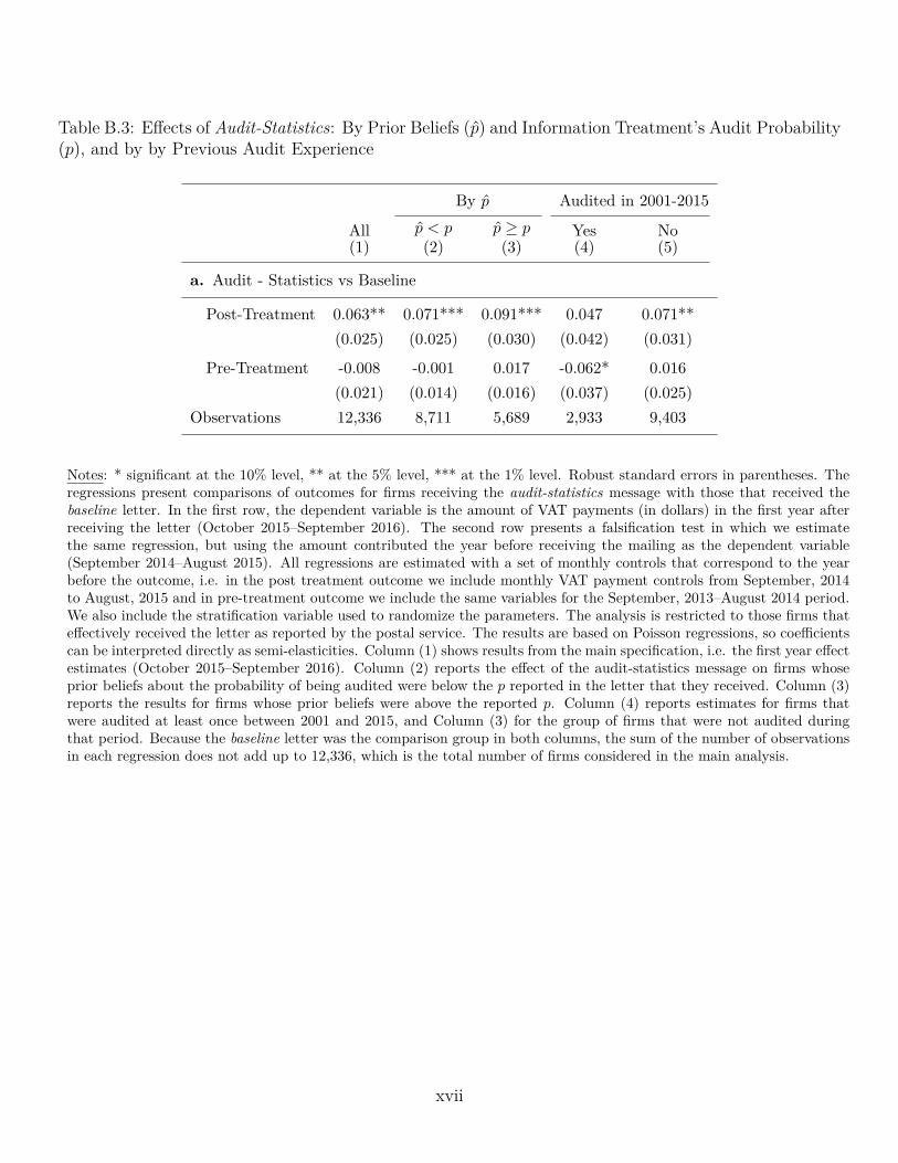
Table B.3: Effects of Audit-Statistics: By Prior Beliefs (p̂) and Information Treatment’s Audit Probability(p), and by by Previous Audit Experience

By p̂ Audited in 2001-2015

All(1)

p̂ < p(2)

p̂ ≥ p(3)

Yes(4)

No(5)

a. Audit - Statistics vs Baseline

Post-Treatment 0.063** 0.071*** 0.091*** 0.047 0.071**(0.025) (0.025) (0.030) (0.042) (0.031)

Pre-Treatment -0.008 -0.001 0.017 -0.062* 0.016(0.021) (0.014) (0.016) (0.037) (0.025)

Observations 12,336 8,711 5,689 2,933 9,403

Notes: * significant at the 10% level, ** at the 5% level, *** at the 1% level. Robust standard errors in parentheses. Theregressions present comparisons of outcomes for firms receiving the audit-statistics message with those that received thebaseline letter. In the first row, the dependent variable is the amount of VAT payments (in dollars) in the first year afterreceiving the letter (October 2015–September 2016). The second row presents a falsification test in which we estimatethe same regression, but using the amount contributed the year before receiving the mailing as the dependent variable(September 2014–August 2015). All regressions are estimated with a set of monthly controls that correspond to the yearbefore the outcome, i.e. in the post treatment outcome we include monthly VAT payment controls from September, 2014to August, 2015 and in pre-treatment outcome we include the same variables for the September, 2013–August 2014 period.We also include the stratification variable used to randomize the parameters. The analysis is restricted to those firms thateffectively received the letter as reported by the postal service. The results are based on Poisson regressions, so coefficientscan be interpreted directly as semi-elasticities. Column (1) shows results from the main specification, i.e. the first year effectestimates (October 2015–September 2016). Column (2) reports the effect of the audit-statistics message on firms whoseprior beliefs about the probability of being audited were below the p reported in the letter that they received. Column (3)reports the results for firms whose prior beliefs were above the reported p. Column (4) reports estimates for firms thatwere audited at least once between 2001 and 2015, and Column (3) for the group of firms that were not audited duringthat period. Because the baseline letter was the comparison group in both columns, the sum of the number of observationsin each regression does not add up to 12,336, which is the total number of firms considered in the main analysis..

xvii

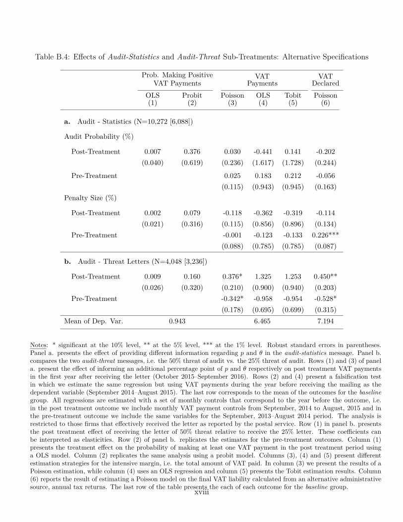
Table B.4: Effects of Audit-Statistics and Audit-Threat Sub-Treatments: Alternative Specifications

Prob. Making PositiveVAT Payments

VATPayments

VATDeclared

OLS(1)

Probit(2)

Poisson(3)

OLS(4)

Tobit(5)

Poisson(6)

a. Audit - Statistics (N=10,272 [6,088])

Audit Probability (%)

Post-Treatment 0.007 0.376 0.030 -0.441 0.141 -0.202(0.040) (0.619) (0.236) (1.617) (1.728) (0.244)

Pre-Treatment 0.025 0.183 0.212 -0.056(0.115) (0.943) (0.945) (0.163)

Penalty Size (%)

Post-Treatment 0.002 0.079 -0.118 -0.362 -0.319 -0.114(0.021) (0.316) (0.115) (0.856) (0.896) (0.134)

Pre-Treatment -0.001 -0.123 -0.133 0.226***(0.088) (0.785) (0.785) (0.087)

b. Audit - Threat Letters (N=4,048 [3,236])

Post-Treatment 0.009 0.160 0.376* 1.325 1.253 0.450**(0.026) (0.320) (0.210) (0.900) (0.940) (0.203)

Pre-Treatment -0.342* -0.958 -0.954 -0.528*(0.178) (0.695) (0.699) (0.315)

Mean of Dep. Var. 0.943 6.465 7.194

Notes: * significant at the 10% level, ** at the 5% level, *** at the 1% level. Robust standard errors in parentheses.Panel a. presents the effect of providing different information regarding p and θ in the audit-statistics message. Panel b.compares the two audit-threat messages, i.e. the 50% threat of audit vs. the 25% threat of audit. Rows (1) and (3) of panela. present the effect of informing an additional percentage point of p and θ respectively on post treatment VAT paymentsin the first year after receiving the letter (October 2015–September 2016). Rows (2) and (4) present a falsification testin which we estimate the same regression but using VAT payments during the year before receiving the mailing as thedependent variable (September 2014–August 2015). The last row corresponds to the mean of the outcomes for the baselinegroup. All regressions are estimated with a set of monthly controls that correspond to the year before the outcome, i.e.in the post treatment outcome we include monthly VAT payment controls from September, 2014 to August, 2015 and inthe pre-treatment outcome we include the same variables for the September, 2013–August 2014 period. The analysis isrestricted to those firms that effectively received the letter as reported by the postal service. Row (1) in panel b. presentsthe post treatment effect of receiving the letter of 50% threat relative to receive the 25% letter. These coefficients canbe interpreted as elasticities. Row (2) of panel b. replicates the estimates for the pre-treatment outcomes. Column (1)presents the treatment effect on the probability of making at least one VAT payment in the post treatment period usinga OLS model. Column (2) replicates the same analysis using a probit model. Columns (3), (4) and (5) present differentestimation strategies for the intensive margin, i.e. the total amount of VAT paid. In column (3) we present the results of aPoisson estimation, while column (4) uses an OLS regression and column (5) presents the Tobit estimation results. Column(6) reports the result of estimating a Poisson model on the final VAT liability calculated from an alternative administrativesource, annual tax returns. The last row of the table presents the each of each outcome for the baseline group.. xviii

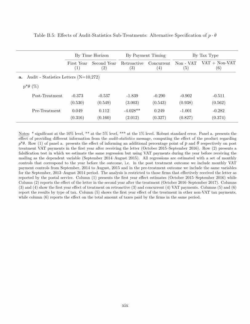
Table B.5: Effects of Audit-Statistics Sub-Treatments: Alternative Specification of p · θ

By Time Horizon By Payment Timing By Tax Type

First Year(1)

Second Year(2)

Retroactive(3)

Concurrent(4)

Non - VAT(5)

VAT + Non-VAT(6)

a. Audit - Statistics Letters (N=10,272)

p*θ (%)

Post-Treatment -0.373 -0.537 -1.839 -0.290 -0.902 -0.511(0.530) (0.549) (3.003) (0.543) (0.938) (0.562)

Pre-Treatment 0.049 0.112 -4.028** 0.249 -1.001 -0.282(0.316) (0.160) (2.012) (0.327) (0.827) (0.374)

Notes: * significant at the 10% level, ** at the 5% level, *** at the 1% level. Robust standard error. Panel a. presents theeffect of providing different information from the audit-statistics message, computing the effect of the product regardingp*θ. Row (1) of panel a. presents the effect of informing an additional percentage point of p and θ respectively on posttreatment VAT payments in the first year after receiving the letter (October 2015–September 2016). Row (2) presents afalsification test in which we estimate the same regression but using VAT payments during the year before receiving themailing as the dependent variable (September 2014–August 2015). All regressions are estimated with a set of monthlycontrols that correspond to the year before the outcome, i.e. in the post treatment outcome we include monthly VATpayment controls from September, 2014 to August, 2015 and in the pre-treatment outcome we include the same variablesfor the September, 2013–August 2014 period. The analysis is restricted to those firms that effectively received the letter asreported by the postal service. Column (1) presents the first year effect estimates (October 2015–September 2016) whileColumn (2) reports the effect of the letter in the second year after the treatment (October 2016–September 2017). Columns(3) and (4) show the first year effect of treatment on retroactive (3) and concurrent (4) VAT payments. Columns (5) and (6)report the results by type of tax. Column (5) shows the first year effect of the treatment in other non-VAT tax payments,while column (6) reports the effect on the total amount of taxes paid by the firms in the same period...

xix

Figure B.1: Distribution of Statistics Shown in Audit-Statistics Lettersa. Audit Probability (p) b. Penalty Rate (θ)

05

1015

2025

Per

cent

0 −

2.49

%

2.5

− 4.

99%

5 −

7.49

%

7.5

− 9.

99%

10 −

12.

49%

12.5

− 1

4.99

%

15 −

17.

49%

17.5

− 1

9.99

%

20 −

22.

49%

22.5

− 2

4.99

%

010

2030

40P

erce

nt

15 −

19.

99%

20 −

24.

99%

25 −

29.

99%

30 −

34.

99%

35 −

39.

99%

40 −

44.

99%

45 −

49.

99%

50 −

54.

99%

55 −

59.

99%

60 −

64.

99%

65 −

69.

99%

Notes: The data corresponds to the distribution of the information provided in the audit-statistics letters (N=10,272).Panel a. presents the distribution of the probability of being audited (p ). Panel b represents the distribution of the averagepenalty rate (θ). p and θ arise from the following procedure: 1) divide the firms in pre-treatment VAT payment quintiles,2) randomly draw a sample of 50 similar firms (i.e. from the same quintile) and 3) compute the average p and θ from thatsample. This algorithm lead to 950 different combinations of the two parameters..

xx

Figure B.2: Effect of audit-statistics vs. baseline, by Prior Beliefsa. Effect of audit probability signal b. Effect of audit probability signal

by quartile of prior beliefs (calibrated to 40.5%) by quartile of prior minus signal (calibrated to 40.5%)

−0.

10−

0.05

0.00

0.05

0.10

0.15

0.20

0.25

Tre

atm

ent E

ffect

0 10 20 30 40 50 60 70Prior Belief: Audit Probability (%)

Point Estimate95% CILinear Fit

−0.

10−

0.05

0.00

0.05

0.10

0.15

0.20

0.25

Tre

atm

ent E

ffect

0 10 20 30 40 50 60Prior Belief: Audit Probability (%)

Point Estimate95% CILinear Fit

Notes: Panel a. (N=11,989) plots the first-year effect (October 2015–September 2016) of the audit-statistics letter ontotal VAT payments by quartiles of prior beliefs while panel b. (N=11,989) reports the same results by quartiles of thedifference between the prior belief and the signal sent in the audit-statistics message. The prior belief is computed asp̂i = 1 −

(1− α0+Ni

α0+β0+Ti

)3where α0 = 1.36 and β0 = 1 such that the mean prior belief about the probability of being

audited at least once in the following three years matches the average probability perceived by firms in the baseline and publicgoods groups according to the survey answers (40.5%). In panel b. the signal for the placebo group was randomly assignedusing the same strategy that for the audit-statistics group. The red dashed line represents the linear fit corresponding tothe estimates for the four quartiles. In panel a, the green dashed line represents the average perceived probability (40.5%)for the comparison group, and in panel b. it represents the point in which prior belief and signal are equal. In both panels,each dot represents the estimated treatment effect for each quartile of the variable considered. Regressions are estimatedusing monthly pre-treatment controls. All effects are depicted with the 95% confidence interval. The results are based onPoisson regressions, so coefficients can be interpreted directly as semi-elasticities. Confidence intervals are computed withrobust standard errors..

xxi

Figure B.3: Effects of Audit-Statistics by Level of the Signal and by Quartera. Effect of audit-statistics vs. baseline, by level of p b. Effect of audit-statistics vs. baseline, by level of θ

−0.

10.

00.

10.

2

Tre

atm

ent E

ffect

−2 −1 +1 +2 +3 +4 +5 +6 +7 +8

Quarter

≥ 11.7% < 11.7%

−0.

10.

00.

10.

2

Tre

atm

ent E

ffect

−2 −1 +1 +2 +3 +4 +5 +6 +7 +8

Quarter

≥ 30.6% < 30.6%

Notes: Panels a. and b. (N=10,272) present the effect of p and θ reported in the audit-statistics messages, dividing thesample by above and below the mean value of the corresponding signal. Each dot in panels a. and b. represents theestimate of the effect of treatment on VAT payments for a specific quarter from two quarters before treatment up to eightquarters after receiving the letter. Red dots in panels a. and b. represent the effect for audit-statistics letter recipients withmessages about p or θ above the mean respectively. Green dots represent the same effect but for those with signals aboutp and θ below the mean respectively. Regressions do not include monthly pre-treatment controls. The results are based onPoisson regressions, so coefficients can be interpreted directly as semi-elasticities. 90% confidence intervals represented byred and green lines are computed with robust standard errors..

xxii

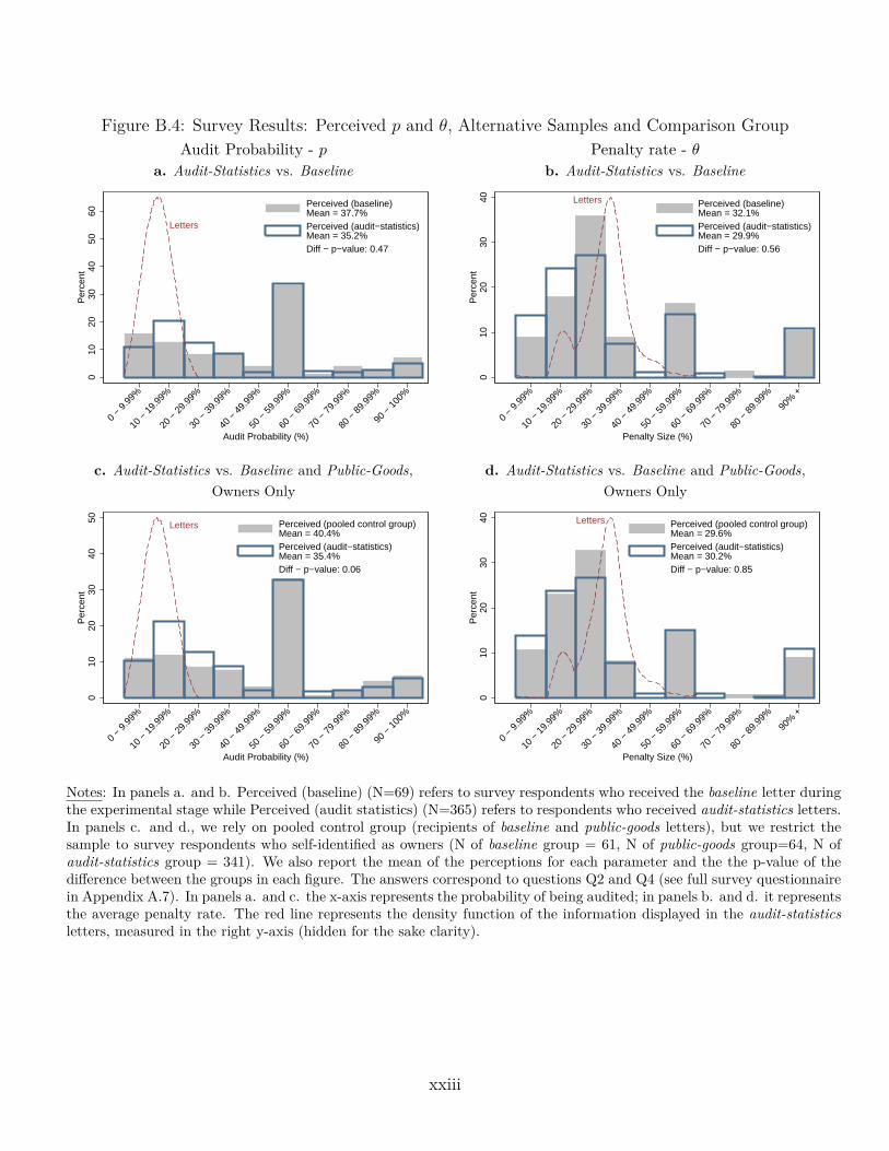
Figure B.4: Survey Results: Perceived p and θ, Alternative Samples and Comparison GroupAudit Probability - p Penalty rate - θ

a. Audit-Statistics vs. Baseline b. Audit-Statistics vs. Baseline

Letters

010

2030

4050

60P

erce

nt

0 −

9.99

%

10 −

19.

99%

20 −

29.

99%

30 −

39.

99%

40 −

49.

99%

50 −

59.

99%

60 −

69.

99%

70 −

79.

99%

80 −

89.

99%

90 −

100

%

Audit Probability (%)

Perceived (baseline)Mean = 37.7%Perceived (audit−statistics)Mean = 35.2%Diff − p−value: 0.47

Letters

010

2030

40P

erce

nt

0 −

9.99

%

10 −

19.

99%

20 −

29.

99%

30 −

39.

99%

40 −

49.

99%

50 −

59.

99%

60 −

69.

99%

70 −

79.

99%

80 −

89.

99%

90%

+

Penalty Size (%)

Perceived (baseline)Mean = 32.1%Perceived (audit−statistics)Mean = 29.9%Diff − p−value: 0.56

c. Audit-Statistics vs. Baseline and Public-Goods, d. Audit-Statistics vs. Baseline and Public-Goods,Owners Only Owners Only

Letters

010

2030

4050

Per

cent

0 −

9.99

%

10 −

19.

99%

20 −

29.

99%

30 −

39.

99%

40 −

49.

99%

50 −

59.

99%

60 −

69.

99%

70 −

79.

99%

80 −

89.

99%

90 −

100

%

Audit Probability (%)

Perceived (pooled control group)Mean = 40.4%Perceived (audit−statistics)Mean = 35.4%Diff − p−value: 0.06

Letters

010

2030

40P

erce

nt

0 −

9.99

%

10 −

19.

99%

20 −

29.

99%

30 −

39.

99%

40 −

49.

99%

50 −

59.

99%

60 −

69.

99%

70 −

79.

99%

80 −

89.

99%

90%

+

Penalty Size (%)

Perceived (pooled control group)Mean = 29.6%Perceived (audit−statistics)Mean = 30.2%Diff − p−value: 0.85

Notes: In panels a. and b. Perceived (baseline) (N=69) refers to survey respondents who received the baseline letter duringthe experimental stage while Perceived (audit statistics) (N=365) refers to respondents who received audit-statistics letters.In panels c. and d., we rely on pooled control group (recipients of baseline and public-goods letters), but we restrict thesample to survey respondents who self-identified as owners (N of baseline group = 61, N of public-goods group=64, N ofaudit-statistics group = 341). We also report the mean of the perceptions for each parameter and the the p-value of thedifference between the groups in each figure. The answers correspond to questions Q2 and Q4 (see full survey questionnairein Appendix A.7). In panels a. and c. the x-axis represents the probability of being audited; in panels b. and d. it representsthe average penalty rate. The red line represents the density function of the information displayed in the audit-statisticsletters, measured in the right y-axis (hidden for the sake clarity)...

xxiii

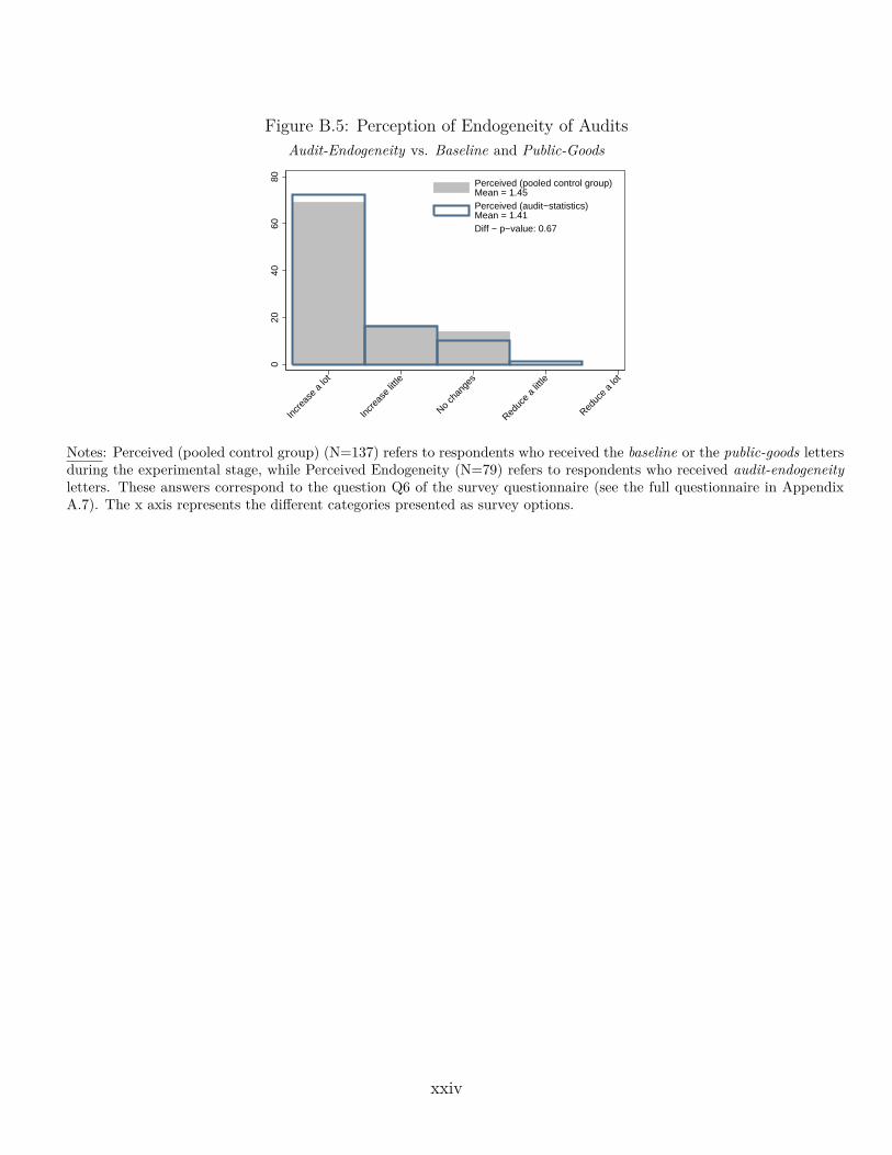
Figure B.5: Perception of Endogeneity of AuditsAudit-Endogeneity vs. Baseline and Public-Goods

020

4060

80

Incr

ease

a lo

t

Incr

ease

little

No ch

ange

s

Reduc

e a

little

Reduc

e a

lot

Perceived (pooled control group)Mean = 1.45Perceived (audit−statistics)Mean = 1.41Diff − p−value: 0.67

Notes: Perceived (pooled control group) (N=137) refers to respondents who received the baseline or the public-goods lettersduring the experimental stage, while Perceived Endogeneity (N=79) refers to respondents who received audit-endogeneityletters. These answers correspond to the question Q6 of the survey questionnaire (see the full questionnaire in AppendixA.7). The x axis represents the different categories presented as survey options..

xxiv

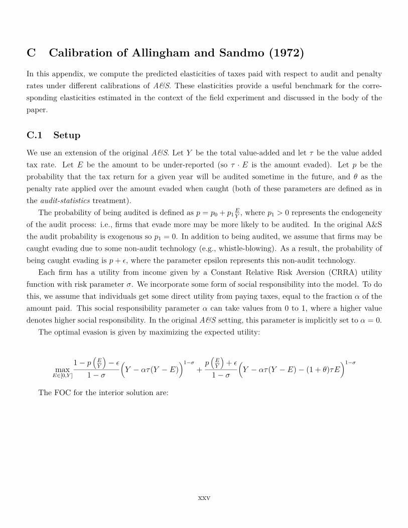
C Calibration of Allingham and Sandmo (1972)

In this appendix, we compute the predicted elasticities of taxes paid with respect to audit and penaltyrates under different calibrations of A&S. These elasticities provide a useful benchmark for the corre-sponding elasticities estimated in the context of the field experiment and discussed in the body of thepaper.

C.1 Setup

We use an extension of the original A&S. Let Y be the total value-added and let τ be the value addedtax rate. Let E be the amount to be under-reported (so τ · E is the amount evaded). Let p be theprobability that the tax return for a given year will be audited sometime in the future, and θ as thepenalty rate applied over the amount evaded when caught (both of these parameters are defined as inthe audit-statistics treatment).

The probability of being audited is defined as p = p0 + p1EY, where p1 > 0 represents the endogeneity

of the audit process: i.e., firms that evade more may be more likely to be audited. In the original A&Sthe audit probability is exogenous so p1 = 0. In addition to being audited, we assume that firms may becaught evading due to some non-audit technology (e.g., whistle-blowing). As a result, the probability ofbeing caught evading is p+ ε, where the parameter epsilon represents this non-audit technology.

Each firm has a utility from income given by a Constant Relative Risk Aversion (CRRA) utilityfunction with risk parameter σ. We incorporate some form of social responsibility into the model. To dothis, we assume that individuals get some direct utility from paying taxes, equal to the fraction α of theamount paid. This social responsibility parameter α can take values from 0 to 1, where a higher valuedenotes higher social responsibility. In the original A&S setting, this parameter is implicitly set to α = 0.

The optimal evasion is given by maximizing the expected utility:

maxE∈[0,Y ]

1− p(EY

)− ε

1− σ

(Y − ατ(Y − E)

)1−σ+p(EY

)+ ε

1− σ

(Y − ατ(Y − E)− (1 + θ)τE

)1−σ

The FOC for the interior solution are:

xxv

(1− p

(E

Y

)− ε

)(Y − ατ(Y − E)

)−σατ −

∂p(EY )∂E

Y (1− σ)

(Y − ατ(Y − E)

)1−σ−

−(p(E

Y

)+ ε

)(Y − ατ(Y − E)− (1 + θ)τE

)−σ(1 + θ − α)τ+

+∂p(EY )∂E

Y (1− σ)

(Y − ατ(Y − E)− (1 + θ)τE

)1−σ= 0

(Y − ατ(Y − E)

)−σ((1− p

(E

Y

)− ε)ατ −

∂p(EY )∂E

Y (1− σ)(Y − ατ(Y − E)))

=

(Y −ατ(Y −E)− (1 + θ)τE

)−σ((p(E

Y

)+ ε

)(1 + θ−α)τ −

∂p(EY )∂E

Y (1− σ)(Y −ατ(Y −E)− (1 + θ)τE))

In the traditional A&S specification, with α = 1, p1 = 0 and ε = 0, we can obtain a closed analyticalform for the elasticities between the VAT payments and p and θ:

∂log (τ(Y − E))∂p

= −(1− τ)− 1σ

(pθ

1−p

)−σ+1σ θ(1+θ)

(1−p)2(θ(pθ

1−p

)− 1σ + 1

)2 (τ − (1− τ)

(( pθ

1−p)− 1σ−1

1+θ( pθ1−p)

− 1σ

))

∂log (τ(Y − E))∂θ

= −(1− τ)−(1 + θ) 1

σ

(pθ

1−p

)−σ+1σ p

1−p −(pθ

1−p

)− 1σ ((pθ

1−p

)− 1σ − 1)(

θ(pθ

1−p

)− 1σ + 1

)2 (τ − (1− τ)

(( pθ

1−p)− 1σ−1

1+θ( pθ1−p)

− 1σ

))

When we expand the model with α < 1 or ε > 0, we can still get closed-form expressions for thesetwo elasticities. However, such elasticities no longer have closed-form solutions when we allow for p1 > 0.In this last case, we use standard numerical methods to compute these elasticities.

C.2 Calibration Results

Table C.1 presents the calibration results. Each row corresponds to a different calibration of A&S.The first seven columns correspond to the parameter values: σ, τ , p0, p1, ε, θ and α. The last threecolumns correspond to the predictions of the model under those parameter values. All the parametersare calibrated so that they always predict an evasion rate (E

Y) of 26%, which corresponds to the average

evasion rate estimated for Uruguay (Gomez-Sabaini and Jimenez, 2012). As a result, all the predictionsin the column corresponding to E

Yare the same. We predict the two elasticities discussed in the section

xxvi

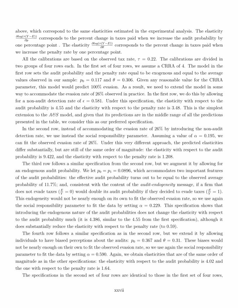
above, which correspond to the same elasticities estimated in the experimental analysis. The elasticity∂log(τ(Y−E))

∂pcorresponds to the percent change in taxes paid when we increase the audit probability by

one percentage point . The elasticity ∂log(τ(Y−E))∂θ

corresponds to the percent change in taxes paid whenwe increase the penalty rate by one percentage point.

All the calibrations are based on the observed tax rate, τ = 0.22. The calibrations are divided intwo groups of four rows each. In the first set of four rows, we assume a CRRA of 4. The model in thefirst row sets the audit probability and the penalty rate equal to be exogenous and equal to the averagevalues observed in our sample: p0 = 0.117 and θ = 0.306. Given any reasonable value for the CRRAparameter, this model would predict 100% evasion. As a result, we need to extend the model in someway to accommodate the evasion rate of 26% observed in practice. In the first row, we do this by allowingfor a non-audit detection rate of ε = 0.581. Under this specification, the elasticity with respect to theaudit probability is 4.55 and the elasticity with respect to the penalty rate is 3.48. This is the simplestextension to the A&S model, and given that its predictions are in the middle range of all the predictionspresented in the table, we consider this as our preferred specification.

In the second row, instead of accommodating the evasion rate of 26% by introducing the non-auditdetection rate, we use instead the social responsibility parameter. Assuming a value of α = 0.195, wecan fit the observed evasion rate of 26%. Under this very different approach, the predicted elasticitiesdiffer substantially, but are still of the same order of magnitude: the elasticity with respect to the auditprobability is 9.422, and the elasticity with respect to the penalty rate is 1.208.

The third row follows a similar specification from the second row, but we augment it by allowing foran endogenous audit probability. We let p0 = p1 = 0.0896, which accommodates two important featuresof the audit probabilities: the effective audit probability turns out to be equal to the observed averageprobability of 11.7%; and, consistent with the content of the audit-endogeneity message, if a firm thatdoes not evade taxes (E

Y= 0) would double its audit probability if they decided to evade taxes (E

Y= 1).

This endogeneity would not be nearly enough on its own to fit the observed evasion rate, so we use againthe social responsibility parameter to fit the data by setting α = 0.229. This specification shows thatintroducing the endogenous nature of the audit probabilities does not change the elasticity with respectto the audit probability much (it is 4.386, similar to the 4.55 from the first specification), although itdoes substantially reduce the elasticity with respect to the penalty rate (to 0.59).

The fourth row follows a similar specification as in the second row, but we extend it by allowingindividuals to have biased perceptions about the audits: p0 = 0.367 and θ = 0.31. These biases wouldnot be nearly enough on their own to fit the observed evasion rate, so we use again the social responsibilityparameter to fit the data by setting α = 0.590. Again, we obtain elasticities that are of the same order ofmagnitude as in the other specifications: the elasticity with respect to the audit probability is 4.02 andthe one with respect to the penalty rate is 1.64.

The specifications in the second set of four rows are identical to those in the first set of four rows,

xxvii

except that we assume a CRRA parameter of 2 instead of a CRRA of 4. The results indicate thatassuming a higher risk aversion provides more conservative estimates, because the lower risk aversioninduces larger elasticities.

In sum, the different specifications produce elasticities with respect to the audit probability between4.02 and 18.857, and elasticities with respect to the penalty rate between 0.66 and 6.60.

xxviii

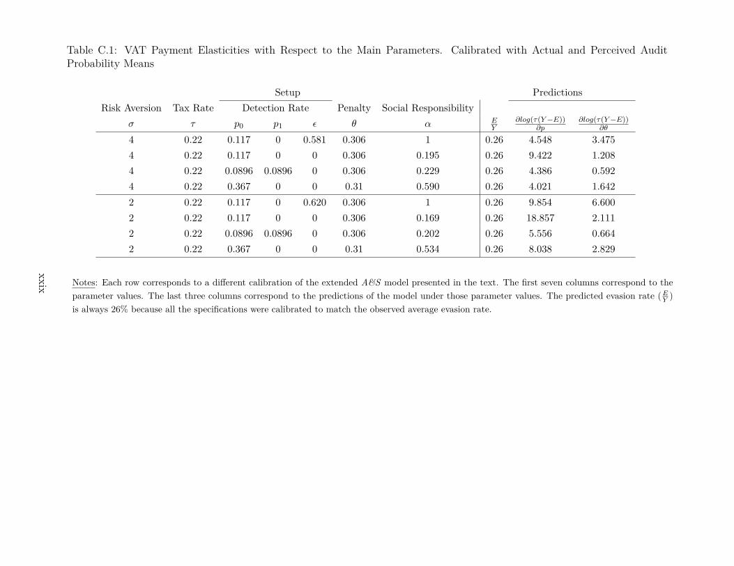
Table C.1: VAT Payment Elasticities with Respect to the Main Parameters. Calibrated with Actual and Perceived AuditProbability Means

Setup PredictionsRisk Aversion Tax Rate Detection Rate Penalty Social Responsibility

σ τ p0 p1 ε θ α EY

∂log(τ(Y−E))∂p

∂log(τ(Y−E))∂θ

4 0.22 0.117 0 0.581 0.306 1 0.26 4.548 3.4754 0.22 0.117 0 0 0.306 0.195 0.26 9.422 1.2084 0.22 0.0896 0.0896 0 0.306 0.229 0.26 4.386 0.5924 0.22 0.367 0 0 0.31 0.590 0.26 4.021 1.6422 0.22 0.117 0 0.620 0.306 1 0.26 9.854 6.6002 0.22 0.117 0 0 0.306 0.169 0.26 18.857 2.1112 0.22 0.0896 0.0896 0 0.306 0.202 0.26 5.556 0.6642 0.22 0.367 0 0 0.31 0.534 0.26 8.038 2.829

Notes: Each row corresponds to a different calibration of the extended A&S model presented in the text. The first seven columns correspond to theparameter values. The last three columns correspond to the predictions of the model under those parameter values. The predicted evasion rate (EY )is always 26% because all the specifications were calibrated to match the observed average evasion rate..

xxix