HAL Id: hal-00872746https://hal.archives-ouvertes.fr/hal-00872746

Submitted on 14 Oct 2013

HAL is a multi-disciplinary open accessarchive for the deposit and dissemination of sci-entific research documents, whether they are pub-lished or not. The documents may come fromteaching and research institutions in France orabroad, or from public or private research centers.

L’archive ouverte pluridisciplinaire HAL, estdestinée au dépôt et à la diffusion de documentsscientifiques de niveau recherche, publiés ou non,émanant des établissements d’enseignement et derecherche français ou étrangers, des laboratoirespublics ou privés.

Dimensional reductions of a cardiac model for effectivevalidation and calibration

Matthieu Caruel, Radomir Chabiniok, Philippe Moireau, Yves Lecarpentier,Dominique Chapelle

To cite this version:Matthieu Caruel, Radomir Chabiniok, Philippe Moireau, Yves Lecarpentier, Dominique Chapelle.Dimensional reductions of a cardiac model for effective validation and calibration. Biomechanics andModeling in Mechanobiology, Springer Verlag, 2014, 13 (4), pp.897-914. <10.1007/s10237-013-0544-6>. <hal-00872746>

Noname manuscript No.(will be inserted by the editor)

Dimensional reductions of a cardiac modelfor effective validation and calibration

M. Caruel · R. Chabiniok · P. Moireau · Y. Lecarpentier · D. Chapelle

the date of receipt and acceptance should be inserted later

Abstract Complex 3D beating heart models are now

available, but their complexity makes calibration and

validation very difficult tasks. We thus propose a sys-

tematic approach of deriving simplified reduced-dimen-

sional models, in “0D” – typically, to represent a car-

diac cavity, or several coupled cavities – and in “1D”

– to model elongated structures such as muscle samples

or myocytes. We apply this approach with an earlier-

proposed 3D cardiac model designed to capture length-

dependence effects in contraction, which we here com-

plement by an additional modeling component devised

to represent length-dependent relaxation. We then pre-

sent experimental data produced with rat papillary mus-

cles samples when varying preload and afterload condi-

tions, and we achieve some detailed validations of the

1D model with these data, including for the length-

dependence effects that are accurately captured. Fi-

nally, when running simulations of the 0D model pre-

calibrated with the 1D model parameters, we obtain

pressure-volume indicators of the left ventricle in good

agreement with some important features of cardiac phys-

iology, including the so-called Frank-Starling mecha-

nism, the End-Systolic Pressure-Volume Relationship

(ESPVR), as well as varying elastance properties. This

integrated multi-dimensional modeling approach thus

sheds new light on the relations between the phenomena

M. Caruel, P. Moireau and D. ChapelleInria Saclay Ile-de-France, MΞDISIM team, Palaiseau,France

R. ChabiniokDivision of Imaging Sciences & Biomedical Engineering,St Thomas’ Hospital, King’s College London, UK

Y. LecarpentierInstitut du Coeur, Hopital de la Pitie-Salpetriere, Paris, andCentre de Recherche Clinique, Hopital de Meaux, France

observed at different scales and at the local vs. organ

levels.

Keywords cardiac modeling; experimental validation;

hierarchical modeling; length-dependence effects;

Frank-Starling mechanism

1 Introduction

Complex three-dimensional (3D) multi-physics beat-

ing heart models are now available – see, e.g., (Peskin,

1975; Nash and Hunter, 2000; Costa et al, 2001; Sachse,

2004; Kerckhoffs et al, 2005; Sainte-Marie et al, 2006;

Niederer and Smith, 2009) and references therein – in-

cluding for patient-specific simulations as in (Smith and

et al., 2011; Chabiniok et al, 2011), themselves based onvarious inverse modeling approaches, see (Schmid et al,

2008; Moireau et al, 2008). However, such models are

computationally intensive, and their physical and com-

putational complexities make their detailed validations

and calibrations difficult. Preliminary calibrations of

the numerous physical parameters are essential to run

meaningful simulations, and to initiate inverse model-

ing loops for personalization purposes, and it is very

ineffective to perform this preliminary stage with the

full 3D model.

Moreover, increasingly sophisticated biomechanical

cardiac tissue models – frequently based on multi-scale

approaches – aim at capturing ever subtler aspects of

the cardiac behavior, whether in physiological or patho-

logical conditions, see e.g. recent survey in (Trayanova

and Rice, 2011). This holds in particular for load-depen-

dence mechanisms, which have been recognized as cru-

cial in cardiac physiology for decades, most notably

with the so-called Frank-Starling effect in contraction

(Frank, 1895; Starling, 1918), and also more recently

2 M. Caruel et al.

in the relaxation stage (Brutsaert et al, 1980). Various

models have endeavored to incorporate such effects, see

e.g. (Panerai, 1980) and references therein for contrac-

tion, and (Izakov et al, 1991; Niederer et al, 2006) for

relaxation. Clearly, as regards the detailed validation of

such refined models, the complete organ is not the ade-

quate scale for model assessments based on experimen-

tal testing, whereas well-adapted controllable protocols

are available at a more local scale, namely, with tissue

samples (Lecarpentier et al, 1979; Kentish et al, 1986;

Parikh et al, 1993), or even myocytes (Bluhm et al,

1995; Cazorla et al, 2000; Iribe et al, 2006). Neverthe-

less, while very refined models can be formulated and

calibrated to reproduce a given family of experiments,

it is also essential that the modeling approach be inte-

grated in a unified framework within which the detailed

3D behavior of the whole organ can also be assessed, in

order to investigate the relations between the behaviors

at the local and global scales.

In this paper we will demonstrate how, using geo-

metrical arguments, a generic 3D model that contains

the most important ingredients to reproduce a proto-

typical cardiac cycle can be used to derive associated

reduced-dimensional models both in “0D” (zero-dimen-

sional) – typically, to represent a cardiac cavity, or sev-

eral coupled cavities – and in “1D” (one-dimensional)

– to model elongated structures such as fibers or my-

ocytes. Such hierarchical models are intended for use

in combination with 3D models to provide dramatic

effectiveness gains without compromising modeling ac-

curacy at the local scale, and we emphasize that our

procedure could easily be applied to many 3D models.

Clearly, whereas the 1D model has a claim to accu-

racy for myocardial structures of adequate geometries,

the 0D model is only meant to provide a straightfor-

ward translation of local properties to the organ level

without incorporating any anatomical details – whereas

other reduced-dimensional approaches such as in (Arts

et al, 1991; Lumens et al, 2009) include more detailed

anatomical descriptions – while the 3D model is avail-

able for accurate simulations of the whole organ. We

emphasize, indeed, that the major originality and po-

tential of our approach lie in that it allows exploiting

a combination of several such closely-related models,

within the hierarchical family thus-constructed, for dif-

ferent purposes such as:

– 1D-0D: to obtain fast translations of experimentally

assessed properties – based on 1D samples – to the

“organ” level approximately represented by the 0D

model;

– 1D-3D: to infer much more accurate translations to

the organ level, e.g. including spatial heterogeneities

and detailed fiber distributions;

– 0D-3D: to easily calibrate the constitutive proper-

ties based on global indicators prior to running 3D

simulations.

We choose to illustrate this dimensional reduction

strategy with the 3D model originally proposed in (Sainte-

Marie et al, 2006) and further refined in (Chapelle et al,

2012), and we then endeavor to use the resulting 1D re-

duced model to assess the modeling framework against

unpublished experimental data obtained with rat papil-

lary muscle samples. The experimental protocol is specif-

ically designed to mimic a cardiac cycle under vary-

ing preload and afterload conditions, in order to more

particularly investigate load-dependence effects. In our

model, systolic effects are accounted for by a function

– proposed in (Chapelle et al, 2012) – representing

the varying number of available cross-bridges with re-

spect to sarcomere strain, which we validate with de-

tailed measured trajectories of extensions and forces,

and also with Hill-type force-velocity curves. Concern-

ing the load-dependence effects occurring in diastole,

we incorporate into the model a new ingredient inspired

from (Izakov et al, 1991).

Once the biophysical model parameters have been

calibrated using the 1D model confronted with papillary

muscles experimental data, we reemploy these parame-

ters – with some limited adaptations – in the 0D model

in order to explore the corresponding behavior of a car-

diac cavity representing a left ventricle. In particular,

we assess the end-systolic pressure-volume relationship

(ESPVR), which our hierarchical modeling strategy al-

lows to directly relate to the length-dependence effects

and Frank-Starling mechanism. We also analyse the re-

sulting behavior in the light of the varying elastance

concept (Suga et al, 1973).

The paper is organized as follows. In Section 2 we

recall the main ingredients of the 3D cardiac model

proposed in (Sainte-Marie et al, 2006; Chapelle et al,

2012). Next, in Section 3 we present the derivation of

the reduced-dimensional 0D and 1D models from the

3D formulation. Then, in Section 4 (Results) we de-

scribe the experimental setup and report on our val-

idation trial based on the 1D model, before assessing

the behavior of the 0D cavity model. These results are

further discussed in Section 5, and we finally give some

concluding remarks in Section 6.

2 3D model summary

We consider the multiscale cardiac model proposed

in (Sainte-Marie et al, 2006; Chapelle et al, 2012), of

which we now summarize the main ingredients, while

Dimensional reductions of a cardiac model for effective validation and calibration 3

also further emphasizing the distinctions that we intro-

duce in this work.

2.1 Sarcomere behavior

Muscles present a multiscale fiber-based structure.

At the microscale, each fiber exhibits a striated aspect

resulting from the succession of contractile units called

sarcomeres. Within the sarcomeres, myosin molecular

motors gathered in so-called thick filaments can peri-

odically attach to the surrounding thinner actin-made

filaments – thus creating so-called cross-bridges – in the

presence of adenosine tri-phosphate (ATP), the metabolic

fuel of cells. The forces exerted via these cross-bridges

by actin-myosin interaction can then induce the relative

sliding of the interdigitated filaments, hence the short-

ening of individual sarcomeres and the macroscopic con-

traction.

We first concentrate on the behavior of the sarcom-

eres and model the kinetics of cross-bridges by using

an extension of A.F. Huxley’s model (Huxley, 1957).

Let us denote by ec the equivalent strain associated

with the relative displacements of actin versus myosin

filaments. All along the thick myosin filaments, the pro-

truding myosin heads can attach to special sites located

on thin actin filaments. For a given myosin head, we

denote by s the distance to the closest such actin site

scaled by a characteristic interspace distance. Assum-

ing that only one site at a time is available for any given

myosin head, we introduce n(s, t) the fraction of heads

attached at a distance s at time t. As long as a head re-

mains attached, its extension s varies at the same rate

as ec, hence,

∂n

∂t+ ec

∂n

∂s=(n0(ec)− n

)f − ng, (1)

where f and g denote binding and unbinding rates,

respectively, and the strain-dependent function n0 ac-

counts for the length-dependent fraction of recruitable

myosin heads, by which we depart from the original

Huxley equation with right-hand side (1 − n)f − ng.

Many earlier works have proposed mechanical mod-

els of muscle contraction based on the Huxley descrip-

tion or variants thereof, albeit in general the intro-

duction of such terms as n0 in (1) primarily aims at

providing a detailed description of calcium dynamics

(Wong, 1972; Zahalak and Ma, 1990), in which some

length-dependence can be optionally introduced (Pan-

erai, 1980). Here, with our focus on mechanical model-

ing we will consider chemical activation as given, and di-

rectly incorporate length dependence into n0. The heart

muscle is known to work on the “ascending limb” of the

force-length relation where the maximum active force

rapidly increases with the degree of myofilament over-

lap within the sarcomeres (Gordon et al, 1966; Fabiato

and Fabiato, 1975; Julian and Sollins, 1975; ter Keurs

et al, 1980; Kentish et al, 1986; Shiels and White, 2008).

This phenomenon – related to the Frank-Starling mech-

anism at the organ level – is of utmost importance for

the cardiac function (Moss and Fitzsimons, 2002; Guy-

ton and Hall, 2011; Tortora and Derrikson, 2009) and

will be characterized by n0(ec) in our model. Moreover,

as in (Bestel et al, 2001; Chapelle et al, 2012) we model

f and g by

f(s, t) = |u|+ 1s∈[0,1]g(s, t) = |u|+ 1s/∈[0,1] + |u|− + α |ec|

(2a)

(2b)

where 1 denotes the indicator function – namely, e.g.,

1s∈[0,1] = 1 for s ∈ [0, 1], and 0 otherwise – and u

denotes a variable reaction rate summarizing chemical

activation – in particular calcium kinetics, see e.g. (Za-

halak and Ma, 1990; Hunter et al, 1998) – inducing

contraction or relaxation depending on whether u is

positive or negative, respectively. We use |u|+ et |u|−to respectively denote the positive and absolute values

of u, namely, |u|+ = u when u ≥ 0 and 0 otherwise,

whereas |u|− = −u when u ≤ 0 and 0 otherwise. The

term α |ec| accounts for bridges destruction upon rapid

length changes, which is revealed by rapid force drop

following fast length change (Izakov et al, 1991).

With this particular choice of f and g, we have f +

g = |u| + α |ec| and we note that this expression is

independent of s, an assumption often used in modeling

actin-myosin interaction (Guerin et al, 2011).

Relaxation is also known to be load-dependent in

mammalian cardiac muscles, with experimental evidence

showing that relaxation occurs earlier at lower loads or

smaller sarcomere lengths (Lecarpentier et al, 1979).

This phenomenon is often attributed to collective ef-

fects induced by an interplay between the ability of

troponin to bind calcium ions and the concentration

of myosin motors, or by steric effects due to changes in

lattice spacing upon contraction (Izakov et al, 1991;

Campbell, 2011), and also by calcium concentration

variations regulated by ion exchangers and sarcoplas-

mic reticulum (Brutsaert et al, 1980). This additional

length-dependence effect motivates that we depart from

the previous formulations (Chapelle et al, 2012; Sainte-

Marie et al, 2006) and represent this phenomenon by

introducing in the spirit of (Izakov et al, 1991) – al-

beit in a simpler summarized manner – a new internal

variable w(t) obeying the first-order dynamics

αrw = m0(ec)− w, (3)

4 M. Caruel et al.

which has a multiplicative effect when u ≤ 0 (relax-

ation), namely,

u = |u(t)|+ − w |u(t)|− , (4)

where u(t) is now an input variable independent of

the sarcomere state. The relaxation load-dependence

is then driven by the function m0 that will be defined

as a decreasing function of ec with a reference value

of 1 at high ec, while the parameter αr is a time con-

stant associated with a simple delay effect pertaining

to the complex chain of underlying chemical processes

summarized in the evolution of w.

The stress state in the sarcomere is then obtained

by assuming here a simple quadratic energy for realized

cross-bridges, in the form

Wm(s) = k02 (s+ s0)2,

namely, a linear spring of stiffness k0 and pre-strain

s0, which induces an individual force k0(s + s0). The

overall stiffness and stress in the sarcomere are thus

respectively given by

kc(t) = k0

∫n(s, t) ds,

τc(t) =

∫W ′m(s)n(s, t) ds = k0

∫(s+ s0)n(s, t) ds,

where we recognize expressions directly associated with

the first two moments of the density function n. The

corresponding moments dynamics are then obtained by

integrating over s in (1), which leads to the following

closed-form dynamical systemkc = −(|u|+ + w |u|− + α |ec|) kc + n0k0 |u|+τc = −(|u|+ + w |u|− + α |ec|) τc + n0σ0 |u|+ + kcec

where σ0 = k0(s0+1/2) represents the maximum active

stress.

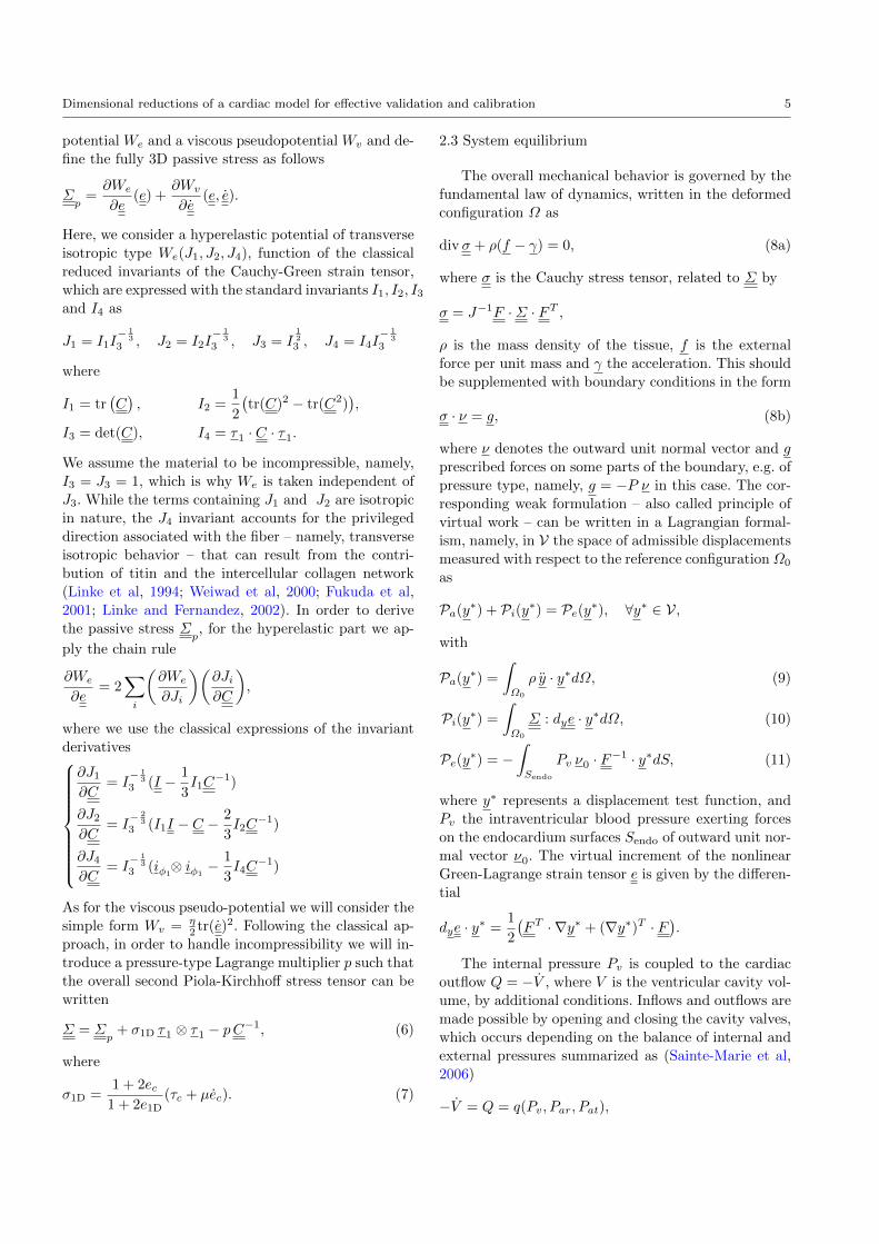
2.2 Overall constitutive law

We denote by y the displacement field with respect

to a stress-free reference configuration Ω0. We then in-

troduce the right Cauchy-Green deformation tensor C,

and the associated Green-Lagrange strain tensor e, de-

fined by

C = FT · F , e =1

2(C − I),

where F = I +∇y is the deformation gradient.

As in (Sainte-Marie et al, 2006; Chapelle et al, 2012),

we use a non-linear Hill-Maxwell rheological law to in-

corporate the above contractile modeling into the over-

all behavior, see Fig.1. As we are pursuing a Lagrangian

Es µ

τc, kc, u

We

η

es (σs) ec (σc)

e

Fig. 1 Hill-Maxwell rheological model

description of the system with a strain measure given

by the Green-Lagrange strain tensor, it is natural to

use the second Piola-Kirchhoff stress tensor for internal

forces, and except when otherwise specified all stress

quantities considered will be associated with this spe-

cific stress tensor. In the first branch of this rheological

schematic, the contractile element is placed in series

with a linear elastic element, and in parallel with a lin-

ear damping element. This whole branch is assumed

to be of 1D character, namely, producing stresses only

along the fiber direction – represented by a spatially-

varying unit vector τ1 – in the form σ1D τ1 ⊗ τ1, in

relation to strains measured along the same direction,

i.e. e1D = τ1 · e · τ1. The parallel association of the

viscous component gives

σc = τc + µec.

with µ a viscous damping parameter. Concerning the

series linearly-elastic element characterized by the stress-

strain law σs = Eses, in our non-linear large strain

framework, the 1D strains e1D, ec and es are related by

1 + 2e1D = (1 + 2es)(1 + 2ec),

while the stresses σ1D, σs and σc obey

σ1D =σs

1 + 2ec=

σc1 + 2es

,

these relations representing the nonlinear extensions

of the usual series-type rheological identities (Chapelle

et al, 2012). This leads to the additional dynamical re-

lation

τc + µec = Es(e1D − ec)(1 + 2e1D)

(1 + 2ec)3. (5)

To take into account the connective tissue surround-

ing the myocardial fiber, we introduce a hyperelastic

Dimensional reductions of a cardiac model for effective validation and calibration 5

potential We and a viscous pseudopotential Wv and de-

fine the fully 3D passive stress as follows

Σp

=∂We

∂e(e) +

∂Wv

∂e(e, e).

Here, we consider a hyperelastic potential of transverse

isotropic type We(J1, J2, J4), function of the classical

reduced invariants of the Cauchy-Green strain tensor,

which are expressed with the standard invariants I1, I2, I3and I4 as

J1 = I1I− 1

33 , J2 = I2I

− 13

3 , J3 = I123 , J4 = I4I

− 13

3

where

I1 = tr(C), I2 =

1

2

(tr(C)2 − tr(C2)

),

I3 = det(C), I4 = τ1 · C · τ1.

We assume the material to be incompressible, namely,

I3 = J3 = 1, which is why We is taken independent of

J3. While the terms containing J1 and J2 are isotropic

in nature, the J4 invariant accounts for the privileged

direction associated with the fiber – namely, transverse

isotropic behavior – that can result from the contri-

bution of titin and the intercellular collagen network

(Linke et al, 1994; Weiwad et al, 2000; Fukuda et al,

2001; Linke and Fernandez, 2002). In order to derive

the passive stress Σp, for the hyperelastic part we ap-

ply the chain rule

∂We

∂e= 2

∑i

(∂We

∂Ji

)(∂Ji∂C

),

where we use the classical expressions of the invariant

derivatives

∂J1∂C

= I− 1

33 (I − 1

3I1C

−1)

∂J2∂C

= I− 2

33 (I1I − C −

2

3I2C

−1)

∂J4∂C

= I− 1

33 (iφ1

⊗ iφ1− 1

3I4C

−1)

As for the viscous pseudo-potential we will consider the

simple form Wv = η2 tr(e)2. Following the classical ap-

proach, in order to handle incompressibility we will in-

troduce a pressure-type Lagrange multiplier p such that

the overall second Piola-Kirchhoff stress tensor can be

written

Σ = Σp

+ σ1D τ1 ⊗ τ1 − pC−1, (6)

where

σ1D =1 + 2ec

1 + 2e1D(τc + µec). (7)

2.3 System equilibrium

The overall mechanical behavior is governed by the

fundamental law of dynamics, written in the deformed

configuration Ω as

div σ + ρ(f − γ) = 0, (8a)

where σ is the Cauchy stress tensor, related to Σ by

σ = J−1F ·Σ · FT ,

ρ is the mass density of the tissue, f is the external

force per unit mass and γ the acceleration. This should

be supplemented with boundary conditions in the form

σ · ν = g, (8b)

where ν denotes the outward unit normal vector and g

prescribed forces on some parts of the boundary, e.g. of

pressure type, namely, g = −P ν in this case. The cor-

responding weak formulation – also called principle of

virtual work – can be written in a Lagrangian formal-

ism, namely, in V the space of admissible displacements

measured with respect to the reference configuration Ω0

as

Pa(y∗) + Pi(y∗) = Pe(y∗), ∀y∗ ∈ V,

with

Pa(y∗) =

∫Ω0

ρ y · y∗dΩ, (9)

Pi(y∗) =

∫Ω0

Σ : dye · y∗dΩ, (10)

Pe(y∗) = −∫Sendo

Pv ν0 · F−1 · y∗dS, (11)

where y∗ represents a displacement test function, and

Pv the intraventricular blood pressure exerting forces

on the endocardium surfaces Sendo of outward unit nor-

mal vector ν0. The virtual increment of the nonlinear

Green-Lagrange strain tensor e is given by the differen-

tial

dye · y∗ =1

2

(FT · ∇y∗ + (∇y∗)T · F

).

The internal pressure Pv is coupled to the cardiac

outflow Q = −V , where V is the ventricular cavity vol-

ume, by additional conditions. Inflows and outflows are

made possible by opening and closing the cavity valves,

which occurs depending on the balance of internal and

external pressures summarized as (Sainte-Marie et al,

2006)

−V = Q = q(Pv, Par, Pat),

6 M. Caruel et al.

where Par denotes the pressure in the aorta or in the

pulmonary artery, depending on the ventricle consid-

ered – i.e., the afterload – Pat is the corresponding atrial

pressure that gives the preload in the filling phase, and

q is a regularized version – for numerical purposes – of

the following ideal behaviorQ ≤ 0 if Pv = Pat (filling)

Q = 0 if Pat ≤ Pv ≤ Par (isovol. phases)

Q ≥ 0 if Pv ≥ Par (ejection)

that we approximate as

Q = Kat(Pv − Pat), if Pv ≤ PatQ = Kp(Pv − Pat), if Pat ≤ Pv ≤ ParQ = Kar(Pv − Par) +Kp(Par − Pat), if Pv ≥ Par

(12)

where the regularizing constants Kat, Kp and Kar must

be chosen such that Kp is much smaller than Kar and

Kat to ensure that the flow is negligible in isovolumic

phases.

Finally, the system is closed by a relation represent-

ing the external circulation, with a so-called two-stage

Windkessel model written asCpPar + (Par − Pd)/Rp = Q

CdPd + (Pd − Par)/Rp = (Pvs − Pd)/Rd

where Cp, Rp, Cd and Rd denote capacitances and re-

sistances of the proximal and distal circulations, Pd de-

notes an additional pressure variable called distal pres-sure, and Pvs is a constant representing the venous sys-

tem pressure.

We can now summarize all the above 3D modeling

equations in the following system

Pa(y∗) + Pi(y∗) = Pe(y∗), ∀y∗ ∈ V

Σ =∂We

∂e+∂Wv

∂e+ σ1Dτ1 ⊗ τ1 − pC

−1

σ1D = Ese1D − ec

(1 + 2ec)2

(τc + µec) = Es(e1D − ec)(1 + 2e1D)

(1 + 2ec)3

kc=−(|u|++ w |u|−+α |ec|) kc+ n0k0 |u|+τc=−(|u|++ w |u|−+α |ec|) τc+ n0σ0 |u|++kcec

− V = Q = q(Pv, Par, Pat)

CpPar + (Par − Pd)/Rp = Q

CdPd + (Pd − Par)/Rp = (Pvs − Pd)/Rd

(13a)

(13b)

(13c)

(13d)

(13e)

(13f)

(13g)

(13h)

(13i)

3 Reduced formulations

Dimensional reduction is a process by which the

dimension of the spatial variables space in which the

model is posed – 3D in our case – is decreased by

making adequate assumptions, kinematical and other-

wise, concerning the dimensions that are “eliminated”

in the reduction process. A prototypical example of this

is provided by structural modeling in mechanics, see

e.g. (Bathe, 1996; Chapelle and Bathe, 2011) and refer-

ences therein. As is well-known in structural mechanics,

indeed, dramatic gains in computational effectiveness

can thus be obtained, together with very limited loss in

accuracy provided the underlying assumptions are ad-

equately justified. The dimensional reduction process,

however, is also known to be quite intricate when non-

linear constitutive equations are considered, a difficulty

that we must address here. In our case we will demon-

strate two such possible reductions:

– 0D model: assuming spherical symmetry we will ob-

tain a 0D model, namely, without any spatial vari-

able; this model aims at approximately representing

a cardiac cavity – the left ventricle, typically – but

of course as spherical symmetry does not hold in

actuality, the model will have limited accuracy, and

in fact is only meant as a fast simulation tool ex-

hibiting adequate trends in behavior, in particular

as regards parameter variations.

– 1D model: assuming cylindrical symmetry and uni-

axial loading we will derive a 1D model; in this case

the reduced model can be very accurate in specific

contexts where the assumptions are justified, such

as experimental testing with ad hoc muscle samples,

as will be considered in Section 4.

We point out that in the latter case such a 1D reduced

model is the best-suited candidate for confronting mus-

cle model simulations to experimental measurements

obtained with cylindrical samples. In fact, a “naive”

use of the 3D model instead – with one finite element

across the thickness, say – would lead to severely er-

roneous modeling results due to fundamental incom-

patibilities between simplified kinematics and the ac-

tual stress state, see (Koiter, 1965; Chapelle and Bathe,

2011). Therefore, in such cases strong 3D mesh refine-

ment would be required, whereas just a few 1D ele-

ments – or even a single element when a homogeneous

behavior is considered – can suffice to provide excellent

accuracy.

We further emphasize that our reduction strategy is

not a simple application of local 3D constitutive equa-

tions in specific configurations, but incorporates essen-

tial modeling ingredients into complete formulations

Dimensional reductions of a cardiac model for effective validation and calibration 7

which retain the character of continuous media dynam-

ics, compatible in particular with relevant boundary

conditions, and with incompressibility constraints. More-

over this approach is generic, and can be applied with

a wide class of models, indeed.

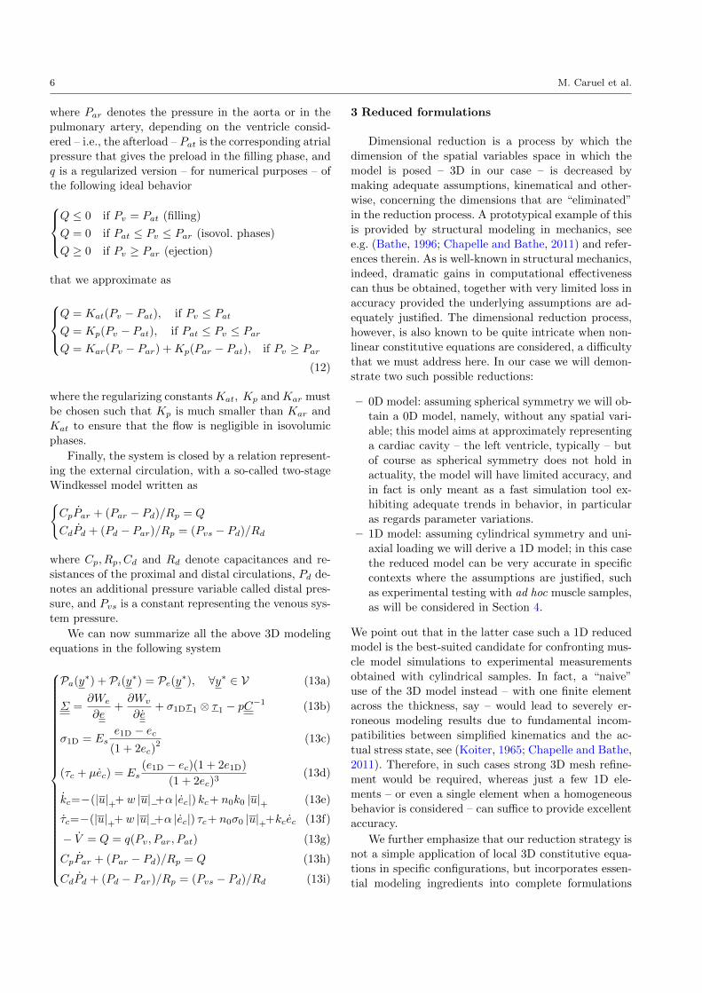
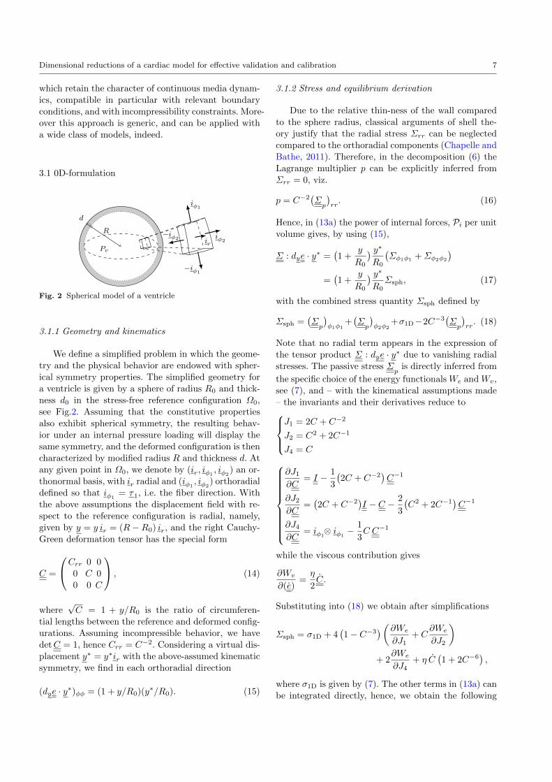
3.1 0D-formulation

R

d

Pv

iφ1

−iφ1

−iφ2 iφ2ir

Fig. 2 Spherical model of a ventricle

3.1.1 Geometry and kinematics

We define a simplified problem in which the geome-

try and the physical behavior are endowed with spher-

ical symmetry properties. The simplified geometry for

a ventricle is given by a sphere of radius R0 and thick-

ness d0 in the stress-free reference configuration Ω0,

see Fig.2. Assuming that the constitutive properties

also exhibit spherical symmetry, the resulting behav-

ior under an internal pressure loading will display the

same symmetry, and the deformed configuration is then

characterized by modified radius R and thickness d. At

any given point in Ω0, we denote by (ir, iφ1, iφ2

) an or-thonormal basis, with ir radial and (iφ1

, iφ2) orthoradial

defined so that iφ1= τ1, i.e. the fiber direction. With

the above assumptions the displacement field with re-

spect to the reference configuration is radial, namely,

given by y = y ir = (R−R0) ir, and the right Cauchy-

Green deformation tensor has the special form

C =

Crr 0 0

0 C 0

0 0 C

, (14)

where√C = 1 + y/R0 is the ratio of circumferen-

tial lengths between the reference and deformed config-

urations. Assuming incompressible behavior, we have

detC = 1, hence Crr = C−2. Considering a virtual dis-

placement y∗ = y∗ir with the above-assumed kinematic

symmetry, we find in each orthoradial direction

(dye · y∗)φφ = (1 + y/R0)(y∗/R0). (15)

3.1.2 Stress and equilibrium derivation

Due to the relative thin-ness of the wall compared

to the sphere radius, classical arguments of shell the-

ory justify that the radial stress Σrr can be neglected

compared to the orthoradial components (Chapelle and

Bathe, 2011). Therefore, in the decomposition (6) the

Lagrange multiplier p can be explicitly inferred from

Σrr = 0, viz.

p = C−2(Σp

)rr. (16)

Hence, in (13a) the power of internal forces, Pi per unit

volume gives, by using (15),

Σ : dye · y∗ =(1 +

y

R0

) y∗R0

(Σφ1φ1

+Σφ2φ2

)=(1 +

y

R0

) y∗R0

Σsph, (17)

with the combined stress quantity Σsph defined by

Σsph =(Σp

)φ1φ1

+(Σp

)φ2φ2

+σ1D−2C−3(Σp

)rr. (18)

Note that no radial term appears in the expression of

the tensor product Σ : dye · y∗ due to vanishing radial

stresses. The passive stress Σp

is directly inferred from

the specific choice of the energy functionals We and Wv,

see (7), and – with the kinematical assumptions made

– the invariants and their derivatives reduce toJ1 = 2C + C−2

J2 = C2 + 2C−1

J4 = C

∂J1∂C

= I − 1

3

(2C + C−2

)C−1

∂J2∂C

=(2C + C−2

)I − C − 2

3

(C2 + 2C−1

)C−1

∂J4∂C

= iφ1⊗ iφ1

− 1

3C C−1

while the viscous contribution gives

∂Wv

∂(e)=η

2C.

Substituting into (18) we obtain after simplifications

Σsph = σ1D + 4(1− C−3

)(∂We

∂J1+ C

∂We

∂J2

)+ 2

∂We

∂J4+ η C

(1 + 2C−6

),

where σ1D is given by (7). The other terms in (13a) can

be integrated directly, hence, we obtain the following

8 M. Caruel et al.

ordinary-differential equation (ODE) for the displace-

ment y

ρd0y +d0R0

(1 +

y

R0

)Σsph = Pv

(1 +

y

R0

)2. (19)

Remark 1 Our spherical symmetry assumption implic-

itly requires an isotropic distribution of the fibers in the

orthoradial directions. Note that there is no contradic-

tion here with the fact that each point can be associated

with a specific fiber direction that corresponds to non-

isotropic mechanical behavior at that particular point.

This simply means that the local distribution of fibers

around that point – e.g. from a probabilistic point of

view – should have no privileged direction within the

orthoradial plane. This is also justified when assuming

that the fiber distribution across the (small) thickness

evenly spans all the directions of this plane.

Finally, the valve law (13g) can be expressed as

−V = 4πR20

(1 +

y

R0

)2y = f

(Pv, Par, Pat

),

so that the initial system (13) finally leads to

ρd0y +d0R0

(1 +

y

R0

)Σsph = Pv

(1 +

y

R0

)2Σsph = σ1D + 4

(1− C−3

)(∂We

∂J1+ C

∂We

∂J2

)+ 2

∂We

∂J4+ 2η C

(1− 2C−6

)σ1D = Es

e1D − ec(1 + 2ec)

2

(τc + µec) = Es(e1D − ec)(1 + 2e1D)

(1 + 2ec)3

kc = −(|u|+ + w |u|− + α |ec|) kc + n0k0 |u|+τc = −(|u|+ + w |u|− + α |ec|) τc + n0σ0 |u|+ + kcec

− V = 4πR20

(1 +

y

R0

)2y = f

(Pv, Par, Pat

)CpPar + (Par − Pd)/Rp = Q

CdPd + (Pd − Par)/Rp = (Psv − Pd)/RdNote that more realistic 0D models could be derived

following similar strategies albeit with more complex

geometric descriptors and kinematical assumptions, see

e.g. Lumens et al (2009), possibly leading to larger sys-

tems of ODEs.

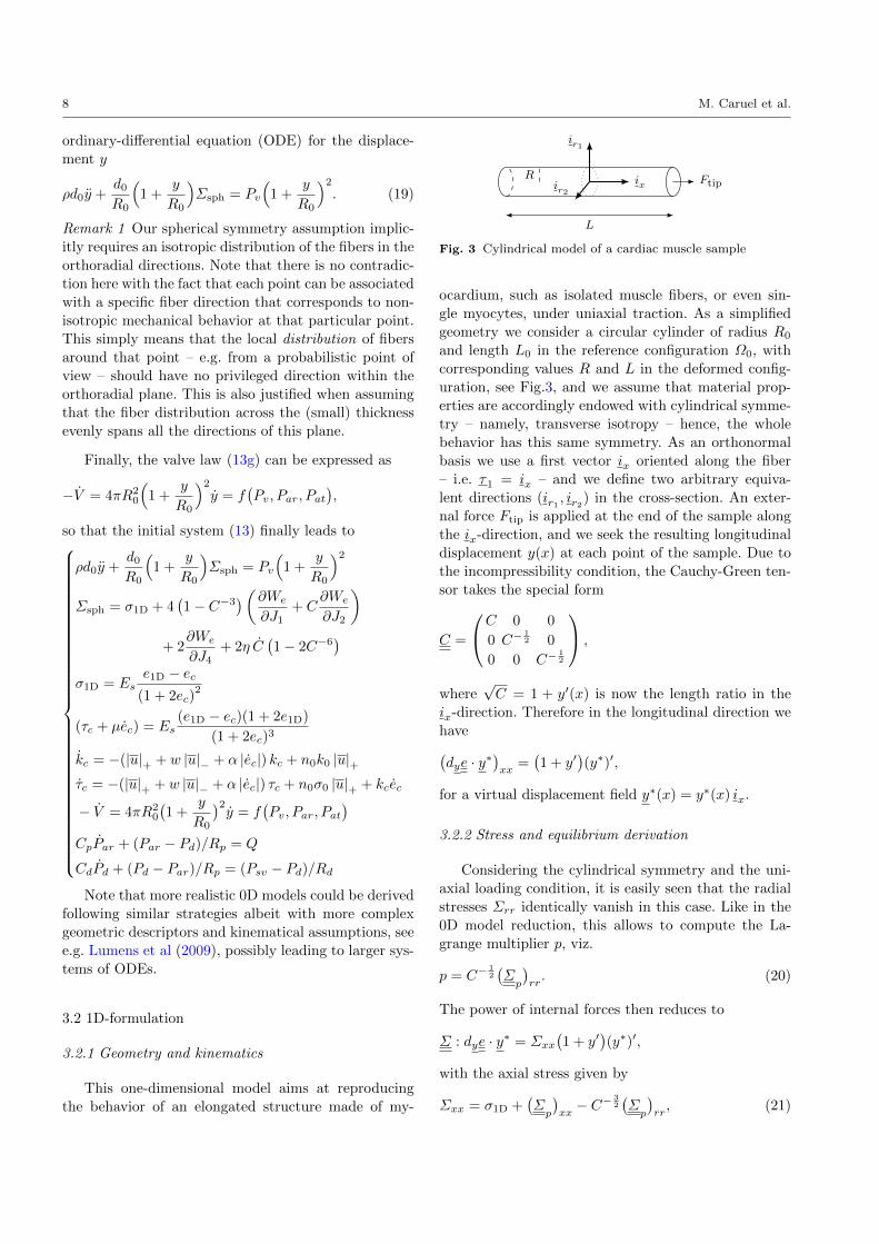
3.2 1D-formulation

3.2.1 Geometry and kinematics

This one-dimensional model aims at reproducing

the behavior of an elongated structure made of my-

ir1

ir2

R ix

L

Ftip

Fig. 3 Cylindrical model of a cardiac muscle sample

ocardium, such as isolated muscle fibers, or even sin-

gle myocytes, under uniaxial traction. As a simplified

geometry we consider a circular cylinder of radius R0

and length L0 in the reference configuration Ω0, with

corresponding values R and L in the deformed config-

uration, see Fig.3, and we assume that material prop-

erties are accordingly endowed with cylindrical symme-

try – namely, transverse isotropy – hence, the whole

behavior has this same symmetry. As an orthonormal

basis we use a first vector ix oriented along the fiber

– i.e. τ1 = ix – and we define two arbitrary equiva-

lent directions (ir1 , ir2) in the cross-section. An exter-

nal force Ftip is applied at the end of the sample along

the ix-direction, and we seek the resulting longitudinal

displacement y(x) at each point of the sample. Due to

the incompressibility condition, the Cauchy-Green ten-

sor takes the special form

C =

C 0 0

0 C−12 0

0 0 C−12

,

where√C = 1 + y′(x) is now the length ratio in the

ix-direction. Therefore in the longitudinal direction we

have(dye · y∗

)xx

=(1 + y′

)(y∗)′,

for a virtual displacement field y∗(x) = y∗(x) ix.

3.2.2 Stress and equilibrium derivation

Considering the cylindrical symmetry and the uni-

axial loading condition, it is easily seen that the radial

stresses Σrr identically vanish in this case. Like in the

0D model reduction, this allows to compute the La-

grange multiplier p, viz.

p = C−12

(Σp

)rr. (20)

The power of internal forces then reduces to

Σ : dye · y∗ = Σxx(1 + y′

)(y∗)′,

with the axial stress given by

Σxx = σ1D +(Σp

)xx− C− 3

2

(Σp

)rr, (21)

Dimensional reductions of a cardiac model for effective validation and calibration 9

with e = e1D = (C − 1)/2. In this case, we have for the

hyperelastic partJ1 = C + 2C−

12

J2 = 2C12 + C−1

J4 = C

and

∂J1∂C

= 1− 1

3

(C + 2C−

12

)C−1

∂J2∂C

=(C + 2C−

12

)I − C − 2

3

(2C

12 + C−1

)C−1

∂J4∂C

= ix⊗ ix −1

3C C−1

The derivative of the viscous pseudo-potential gives

∂Wv

∂e=η

2C.

Then we can rewrite (21) as

Σxx = σ1D + 2(1− C− 3

2

)(∂We

∂J1+ C−

12∂We

∂J2

)+ 2

∂We

∂J4+η

2C(1 +

1

2C−

94

),

and finally we can integrate over each cross-section in

(13a), which yields∫ L0

0

[ρ yy∗ +Σxx

(1 + y′

)(y∗)′

]dx =

Ftip

A0y∗(L0),

with A0 = πR20. As Ftip is assumed to be prescribed

here, we are eventually left with the following system

∫ L0

0

[ρ yy∗+Σxx

(1 + y′

)(y∗)′

]dx =

Ftip

A0y∗(L0), ∀y∗∈V

Σxx = σ1D + 2(1− C− 3

2

)(∂We

∂J1+ C−

12∂We

∂J2

)+ 2

∂We

∂J4+η

2C(1 + C−

94

)σ1D = Es

e1D − ec(1 + 2ec)

2

(τc + µec) = Es(e1D − ec)(1 + 2e1D)

(1 + 2ec)3

kc = −(|u|+ + w |u|− + α |ec|) kc + n0k0 |u|+τc = −(|u|+ + w |u|− + α |ec|) τc + n0σ0 |u|+ + kcec

Note that – when integrating by parts in the variational

formulation – we can derive the equivalent strong form

of the mechanical equilibrium, namely,ρy −

[Σxx

(1 + y′

)]′= 0

Σxx(L0)(1 + y′(L0)) =Ftip

A0

(22a)

(22b)

which represents the counterpart of Eqs. (8a)-(8b).

Remark 2 Cylindrical symmetry is a rather strong as-

sumption, but if we only assume axisymmetry together

with “small thickness”, classical structural mechanics

arguments also lead to vanishing radial stresses, hence

a very similar derivation can be performed and the re-

sulting 1D weak form simply reads∫ L0

0

A(x)[ρ yy∗ +Σxx

(1 + y′

)(y∗)′

]dx = Ftipy

∗(L0),

with a non-constant cross-section area parameter A(x).

4 Results

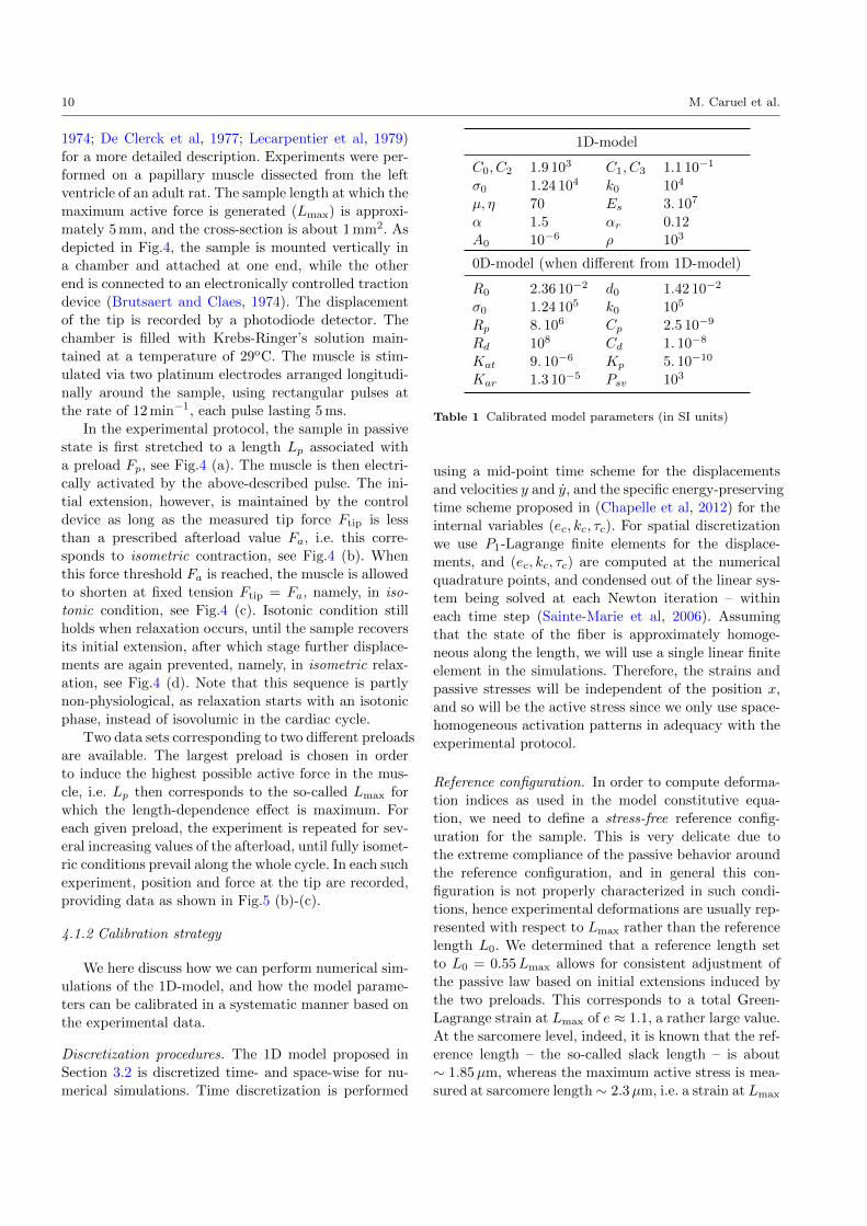
4.1 Application of the 1D model

We illustrate the use of the above-derived 1D model

to represent the behavior of an isolated papillary muscle

sample in experimental conditions designed to mimic

a cardiac cycle (Sonnenblick, 1962; Lecarpentier et al,

1979). This experimental assessment will concurrently

serve the purposes of parameter calibration and model

validation, including for fine features such as length-

dependent effects. We will then demonstrate how the

corresponding calibration can be used in combination

with our dimensional reduction strategy to set up a 0D

model of cardiac contraction.

(a) passive

τc = 0

Ftip = Fp

Lp

(b) isometric

τc > 0

e = 0

Fp < Ftip < Fa

(c) isotonic

τc > 0

e 6= 0

Ftip = Fa

(d) isometric

τc → 0

e = 0

Ftip < Fa

Fig. 4 Experimental protocol for papillary muscle. (a) pas-sive stretching by preload Fp; (b) isometric contraction; (c)isotonic contraction and relaxation against prescribed after-load Fa; (d) isometric relaxation

4.1.1 Experimental data

We start by briefly describing our experimental pro-

tocol before considering the calibration of our 1D-model,

see (Claes and Brutsaert, 1971; Brutsaert and Claes,

10 M. Caruel et al.

1974; De Clerck et al, 1977; Lecarpentier et al, 1979)

for a more detailed description. Experiments were per-

formed on a papillary muscle dissected from the left

ventricle of an adult rat. The sample length at which the

maximum active force is generated (Lmax) is approxi-

mately 5 mm, and the cross-section is about 1 mm2. As

depicted in Fig.4, the sample is mounted vertically in

a chamber and attached at one end, while the other

end is connected to an electronically controlled traction

device (Brutsaert and Claes, 1974). The displacement

of the tip is recorded by a photodiode detector. The

chamber is filled with Krebs-Ringer’s solution main-

tained at a temperature of 29oC. The muscle is stim-

ulated via two platinum electrodes arranged longitudi-

nally around the sample, using rectangular pulses at

the rate of 12 min−1, each pulse lasting 5 ms.

In the experimental protocol, the sample in passive

state is first stretched to a length Lp associated with

a preload Fp, see Fig.4 (a). The muscle is then electri-

cally activated by the above-described pulse. The ini-

tial extension, however, is maintained by the control

device as long as the measured tip force Ftip is less

than a prescribed afterload value Fa, i.e. this corre-

sponds to isometric contraction, see Fig.4 (b). When

this force threshold Fa is reached, the muscle is allowed

to shorten at fixed tension Ftip = Fa, namely, in iso-

tonic condition, see Fig.4 (c). Isotonic condition still

holds when relaxation occurs, until the sample recovers

its initial extension, after which stage further displace-

ments are again prevented, namely, in isometric relax-

ation, see Fig.4 (d). Note that this sequence is partly

non-physiological, as relaxation starts with an isotonic

phase, instead of isovolumic in the cardiac cycle.

Two data sets corresponding to two different preloads

are available. The largest preload is chosen in order

to induce the highest possible active force in the mus-

cle, i.e. Lp then corresponds to the so-called Lmax for

which the length-dependence effect is maximum. For

each given preload, the experiment is repeated for sev-

eral increasing values of the afterload, until fully isomet-

ric conditions prevail along the whole cycle. In each such

experiment, position and force at the tip are recorded,

providing data as shown in Fig.5 (b)-(c).

4.1.2 Calibration strategy

We here discuss how we can perform numerical sim-

ulations of the 1D-model, and how the model parame-

ters can be calibrated in a systematic manner based on

the experimental data.

Discretization procedures. The 1D model proposed in

Section 3.2 is discretized time- and space-wise for nu-

merical simulations. Time discretization is performed

1D-model

C0, C2 1.9 103 C1, C3 1.1 10−1

σ0 1.24 104 k0 104

µ, η 70 Es 3. 107

α 1.5 αr 0.12

A0 10−6 ρ 103

0D-model (when different from 1D-model)

R0 2.36 10−2 d0 1.42 10−2

σ0 1.24 105 k0 105

Rp 8. 106 Cp 2.5 10−9

Rd 108 Cd 1. 10−8

Kat 9. 10−6 Kp 5. 10−10

Kar 1.3 10−5 Psv 103

Table 1 Calibrated model parameters (in SI units)

using a mid-point time scheme for the displacements

and velocities y and y, and the specific energy-preserving

time scheme proposed in (Chapelle et al, 2012) for the

internal variables (ec, kc, τc). For spatial discretization

we use P1-Lagrange finite elements for the displace-

ments, and (ec, kc, τc) are computed at the numerical

quadrature points, and condensed out of the linear sys-

tem being solved at each Newton iteration – within

each time step (Sainte-Marie et al, 2006). Assuming

that the state of the fiber is approximately homoge-

neous along the length, we will use a single linear finite

element in the simulations. Therefore, the strains and

passive stresses will be independent of the position x,

and so will be the active stress since we only use space-

homogeneous activation patterns in adequacy with theexperimental protocol.

Reference configuration. In order to compute deforma-

tion indices as used in the model constitutive equa-

tion, we need to define a stress-free reference config-

uration for the sample. This is very delicate due to

the extreme compliance of the passive behavior around

the reference configuration, and in general this con-

figuration is not properly characterized in such condi-

tions, hence experimental deformations are usually rep-

resented with respect to Lmax rather than the reference

length L0. We determined that a reference length set

to L0 = 0.55Lmax allows for consistent adjustment of

the passive law based on initial extensions induced by

the two preloads. This corresponds to a total Green-

Lagrange strain at Lmax of e ≈ 1.1, a rather large value.

At the sarcomere level, indeed, it is known that the ref-

erence length – the so-called slack length – is about

∼ 1.85µm, whereas the maximum active stress is mea-

sured at sarcomere length∼ 2.3µm, i.e. a strain at Lmax

Dimensional reductions of a cardiac model for effective validation and calibration 11

of e ≈ 0.3. This discrepancy may be explained by the

presence of a compliant series element due to damaged

tissue near the clamps, as already reported in (Krueger

and Pollack, 1975; ter Keurs et al, 1980). In order to

discriminate the effect of such a component, hence to

identify its constitutive behavior, we would need simul-

taneous measurements of sarcomere extensions, which

is out of the scope of the present study. Therefore we

will pursue our calibration with the above-presented

model alone.

−0.5 0 0.5 1 1.5

0

1

2

3

1

23

e

Ftip/A

0(·1

04Pa)

Passive law

Active stress

Preloads

Afterloads

Passive stresses

0 0.2 0.4

1

1.5

1

23

2

1

time (s)

Ftip/A

0(·1

04Pa)

(b)

0 0.2 0.40.7

0.8

0.9

1

1.11 2

3

2 1

time (s)

e

(c)

(a)

Fig. 5 Calibration of passive and active behavior based onpassive extension and maximum active shortening data (a) forhigh/intermediate values of the preload in red/blue, extractedfrom typical dynamical measurements for tip forces (b) andstrains (c); note: example measurement points marked in (b)-(c) are reproduced in (a)

Calibration of the passive behavior law. We calibrate

the passive behavior based on the maximum extension

points shown in Fig.5 (a) for the two different preload

levels (see blue and red squares). The hyperelastic po-

tential We is taken in the form

We = C0 exp(C1(J1 − 3)2

)+ C2 exp

(C3(J4 − 1)2

),

inspired from (Holzapfel and Ogden, 2009), and the pa-

rameters C0, C1, C2 and C3 are chosen to match the

experimental control points, see solid line in Fig.5 (a).

We gather the calibrated parameters in Tab.1. Note

that with the above type of hyperelastic potential ex-

pression, it is not possible to discriminate the parameter

values from the two separate exponential terms based

on uniaxial type measurements alone. Therefore, we

perform this calibration while enforcing the constraint

C0 = C2 and C1 = C3.

Calibration of the length-dependence effect. The next

step consists in the calibration of the length-dependence

effect, represented by the function n0(ec). In Fig.5 (a),

the filled circles represent the state of the system at

maximum shortening under isotonic conditions, namely,

the points labeled “3” in the sub-figures (b) and (c). In

the context of the heart function, this relation is termed

the End Systolic Pressure-Volume Relation (ESPVR).

Here, we denote by esys and esysc the corresponding “end

systolic” values of e and ec, respectively. This state is

characterized by the mechanical equilibrium between

the active stress, the passive stress and the afterload Faexpressed by combining (21) and (22b), which yields

σ1D =Ftip

C12A0

−Σp, Σp =(Σp

)xx

+C−32

(Σp

)rr, (23)

where Σp denotes the passive part of the second Piola-

Kirchhoff stress – here 1D, recall (21) – which can be

directly inferred from the strain esys. Hence, (23) gives

σ1D for each “end-systolic” point. Since σ1D also satis-

fies (13c), we can compute the internal strain esysc . In the

mechanical equilibrium considered, τc+µec = n0(ec)σ0,

hence Eq.(7) can be rewritten as

n0(esysc )σ0 = σ1D1 + 2esys

1 + 2esysc,

which allows to compute the quantity n0(esysc )σ0 for any

given afterload of associated total strain esys. The con-

stant σ0 is inferred from the experimental data at large

preload when the device adjusted so that the entire

process is isometric (i.e. afterload as large as needed),

and using the modeling assumption that n0(ec) = 1,

namely, the maximum value for this state. Finally, the

function n0 is then calibrated from all other experimen-

tal points using a piecewise linear form, see Fig.6 where

we display this function calibrated for several choices of

the series elastic modulus Es.

Influence of finite Es coefficient. The effect of having

a “finite” value for the series elasticity modulus Es –

namely, a value comparable to σ0 – is that the total

strain esys differs from the strain of the active compo-

nent esysc . In Fig.6, we illustrate this effect by showing

the calibrated length-dependence function n0(esysc ) and

the relation esys vs. esysc for different values of Es, while

keeping the same definition of the reference configura-

tion. We can see that the ascending part of the function

n0(esysc ) becomes steeper as Es decreases, which implies

12 M. Caruel et al.

0 1 2

0

0.5

1

esysc

n0

0 2 40

2

4

esysc

esys

(a) (b)

Fig. 6 Influence of Es on the static calibration: blue solidline for infinite Es; red dashed for Es = 3.105 Pa; green dot-dashed for Es = 7.104 Pa

that the course of ec during contraction becomes larger

for a given afterload, since we start from ec = e with

the extension of the preload. Nevertheless, the calibra-

tion of Es would require specific data based on measure-

ments of the sarcomere extensions for various controlled

levels of active forces, see e.g. (Linari et al, 2004, 2007,

2009; Piazzesi et al, 2007). Since we do not have such

data at hand in our case, we use a large value of Es in

the rest of this study.

Calibration of activation. The kinetics of contraction

strongly depend on the activation function u via u, see

(4). As stated in the model presentation, this function

represents a variable reaction rate, and in fact sum-

marizes various complex chemical mechanisms that oc-

cur during depolarization and repolarization (Chapelle

et al, 2012). In practice, we essentially need to prescribe

in u two nominal values characteristic of the time con-

stants of active stress buildup and decay during these

two stages, respectively – with a negative sign for re-

polarization by construction of our active law – with

some transients ensuring continuous evolution through-

out. This leads to a natural description of the function

as piece-wise linear with two plateaus associated with

the depolarization and repolarization rates. Note that

of course alternative parametrizations of similar activa-

tion functions could be considered, e.g. with smoother

exponential functions, albeit limited impact is to be

expected in view of the above considerations on the

activation function behavior. We then adjust this acti-

vation function so that the isometric stress curve cor-

responds to experimental measurements, see Fig.7 for

the calibrated function. Note that, in particular, the

point of maximum tip force must correspond to u = 0,

and subsequent negative values of u induce an extension

via a decrease of the active force. Moreover, the mini-

mum (negative) value of u is obtained from the slope

of the stress relaxation curve in complete isometry for

the large preload, choosing m0(ec) = 1 in this case.

We point out that the maximum (positive) value of u

around 30 s−1 – the inverse of a time constant – is com-

patible with typical ATP turnover time scales (Lymn

and Taylor, 1971; Linari et al, 2010). We further em-

phasize that the activation function u is calibrated once

and for all with a single isometric force measurement,

and then used as is in all subsequent simulations with

varying preloads and afterloads. This activation func-

tion is thus representative of the electric state prevail-

ing in the experimental setup, which is quite different

from what occurs in rat hearts in vivo, in terms of time

constants, in particular (heart rate at rest is about 300

bpm).

Load-dependent relaxation. Once the activation is cali-

brated, we adjust the parameters controlling the load-

dependence of relaxation, namely, via the functionm0(ec),

the time constant αr, and the parameter α control-

ling the velocity-dependent destruction of bridges. We

point out that the isotonic extension phase necessar-

ily corresponds to the late part of the plateau on the

force curves, plateau which ends at the precise moment

when the muscle tip re-establishes the contact with the

support. Therefore, m0 and α together govern the du-

ration of isotonic extension depending on the afterload

– via m0 – and on the preload due to α, since extension

will be larger to reach the support corresponding to a

large preload, see Fig.8. After that, in isometric relax-

ation the force relaxation rate is directly governed by

m0 alone. We set αr to a rather large value, see Tab.1,

hence m0 essentially depends on the end-systolic strain

during the whole relaxation, and then the above consid-

erations allow to calibrate m0 and α based on the data

corresponding to different preloads and afterloads.

0 1 2

0

0.5

1

n0

ec

n0

1

1.2

1.4

1.6

m0

m0

0 0.2 0.4−20

0

20

40

time (s)

u

(a) (b)

Fig. 7 (a) Length-dependence function n0 (solid line) andload dependent relaxation m0 (red dashed line); (b) activationfunction

4.1.3 1D simulation results

Fig.8 shows the dynamics of strain e and tension

Ftip/A0, as simulated by the 1D-model (solid lines) and

compared to experimental data for the two different

preloads (dashed lines), while Fig.9 shows the Hill-type

Dimensional reductions of a cardiac model for effective validation and calibration 13

0

0.5

1

e

High preload Low preload

0 0.2 0.4

0

1

2

3

time (s)

Ftip/A

0(·1

04Pa)

0 0.2 0.4

time (s)

(a)

(b)

(c) (d)

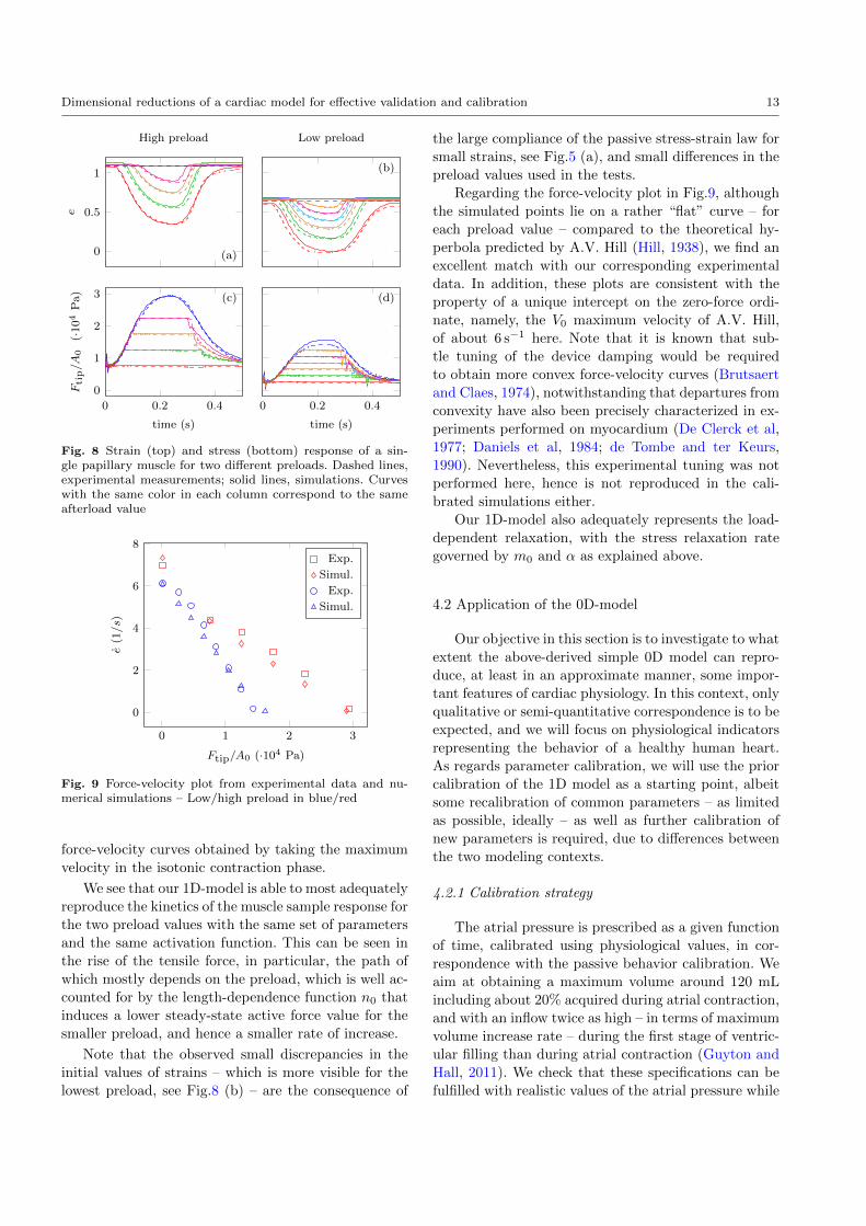
Fig. 8 Strain (top) and stress (bottom) response of a sin-gle papillary muscle for two different preloads. Dashed lines,experimental measurements; solid lines, simulations. Curveswith the same color in each column correspond to the sameafterload value

0 1 2 3

0

2

4

6

8

Ftip/A0 (·104 Pa)

e(1/s)

Exp.

Simul.

Exp.

Simul.

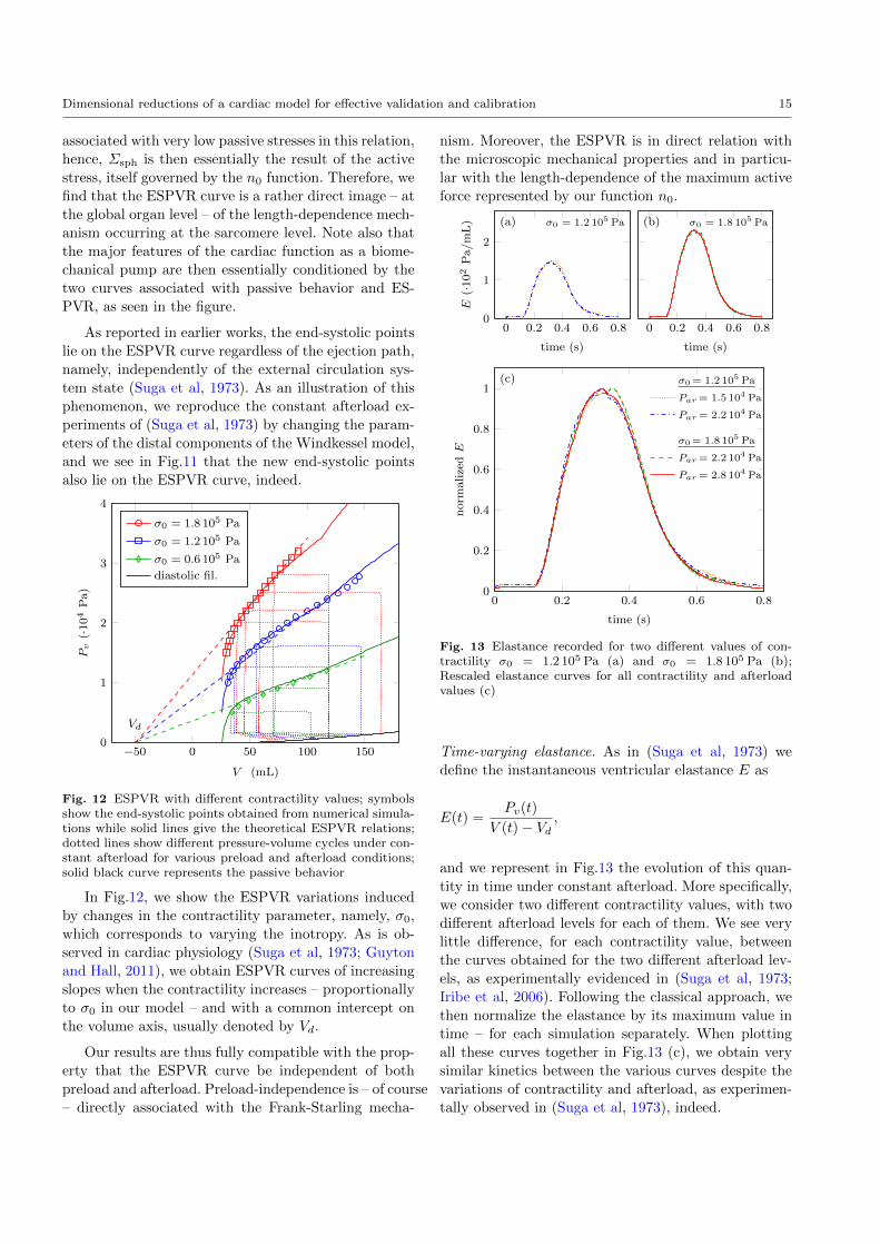
Fig. 9 Force-velocity plot from experimental data and nu-merical simulations – Low/high preload in blue/red

force-velocity curves obtained by taking the maximum

velocity in the isotonic contraction phase.

We see that our 1D-model is able to most adequately

reproduce the kinetics of the muscle sample response for

the two preload values with the same set of parameters

and the same activation function. This can be seen in

the rise of the tensile force, in particular, the path of

which mostly depends on the preload, which is well ac-

counted for by the length-dependence function n0 that

induces a lower steady-state active force value for the

smaller preload, and hence a smaller rate of increase.

Note that the observed small discrepancies in the

initial values of strains – which is more visible for the

lowest preload, see Fig.8 (b) – are the consequence of

the large compliance of the passive stress-strain law for

small strains, see Fig.5 (a), and small differences in the

preload values used in the tests.

Regarding the force-velocity plot in Fig.9, although

the simulated points lie on a rather “flat” curve – for

each preload value – compared to the theoretical hy-

perbola predicted by A.V. Hill (Hill, 1938), we find an

excellent match with our corresponding experimental

data. In addition, these plots are consistent with the

property of a unique intercept on the zero-force ordi-

nate, namely, the V0 maximum velocity of A.V. Hill,

of about 6 s−1 here. Note that it is known that sub-

tle tuning of the device damping would be required

to obtain more convex force-velocity curves (Brutsaert

and Claes, 1974), notwithstanding that departures from

convexity have also been precisely characterized in ex-

periments performed on myocardium (De Clerck et al,

1977; Daniels et al, 1984; de Tombe and ter Keurs,

1990). Nevertheless, this experimental tuning was not

performed here, hence is not reproduced in the cali-

brated simulations either.

Our 1D-model also adequately represents the load-

dependent relaxation, with the stress relaxation rate

governed by m0 and α as explained above.

4.2 Application of the 0D-model

Our objective in this section is to investigate to what

extent the above-derived simple 0D model can repro-

duce, at least in an approximate manner, some impor-

tant features of cardiac physiology. In this context, only

qualitative or semi-quantitative correspondence is to be

expected, and we will focus on physiological indicators

representing the behavior of a healthy human heart.

As regards parameter calibration, we will use the prior

calibration of the 1D model as a starting point, albeit

some recalibration of common parameters – as limited

as possible, ideally – as well as further calibration of

new parameters is required, due to differences between

the two modeling contexts.

4.2.1 Calibration strategy

The atrial pressure is prescribed as a given function

of time, calibrated using physiological values, in cor-

respondence with the passive behavior calibration. We

aim at obtaining a maximum volume around 120 mL

including about 20% acquired during atrial contraction,

and with an inflow twice as high – in terms of maximum

volume increase rate – during the first stage of ventric-

ular filling than during atrial contraction (Guyton and

Hall, 2011). We check that these specifications can be

fulfilled with realistic values of the atrial pressure while

14 M. Caruel et al.

leaving the passive behavior parameters as calibrated

with the 1D model and data.

The active behavior is recalibrated in order to ob-

tain physiological end-systolic states, namely, values of

pressure and volume – with adequate ejection fraction,

in particular – and the slope of the locus of these end-

systolic states in the pressure-volume diagram for vary-

ing afterload levels, i.e. the above-discussed ESPVR. To

that purpose we only modify the contractility param-

eter σ0, which is taken about one order of magnitude

larger in the 0D case. We discuss some possible expla-

nations for this difference in calibration below. We em-

phasize that the activation function u – including the

relaxation modeling components in (3)-(4) – and the

length-dependence n0 function are left unchanged.

In addition, we here need to calibrate the circulation

model. First the distal circulation parameters, Rd and

Cd, are chosen so that the characteristic time of the evo-

lution of the distal pressure Pd – with the time constant

given by RdCd – is compatible with the cycle duration,

i.e. 0.8 s here, while Cd alone governs the distal pressure

increase. Likewise, the proximal parameters Rp and Cpare adjusted so that the associated time constant is

about 10−2 s and the proximal resistance Rp conditions

the peak ventricular pressure. The parameters of the

valve law are chosen so that the pressure-flow relation-

ship (12) is as close as possible to the ideal behavior

without leading to numerical difficulties (Sainte-Marie

et al, 2006).

The final values of the calibrated parameters are

listed in Tab.1.

4.2.2 Simulation results with the 0D-model

Typical cardiac cycle. In Fig.10, we plot the results ob-

tained with the 0D-model. We find that our 0D-model

produces a realistic contraction cycle representative of

a normal human left ventricle, with – in particular – a

physiological ejection fraction of about 60%, and the

maximum filling inflows (negative peaks in Fig.10 (b))

in the above-discussed proportion. As this simulation

was obtained with a straightforward recalibration of

the model validated using the papillary muscle exper-

iments, this confirms the rather direct correspondence

between local properties and a macroscopic organ model.

ESPVR assessment. The ESPRV is one of the most fre-

quently used indicators in normal and pathological car-

diac physiology to assess the cardiac condition. This re-

lation has been shown to be independent of the preload

and afterload (Gordon et al, 1966). We can obtain the

corresponding pressure-volume curve by considering the

0 0.2 0.4 0.6 0.80.4

0.6

0.8

1

1.2

time (s)

V(·1

0−4m

3)

0 0.2 0.4 0.6 0.8

−5

0

5

time (s)

Q(·1

0−4m

3/s)

0 0.2 0.4 0.6 0.80

0.5

1

1.5

time (s)

Pv(·1

04Pa)

0.4 0.6 0.8 1 1.20

0.5

1

1.5

V (·10−4 m3)

Pv(·1

04Pa)

(a) (b)

(c) (d)

Fig. 10 Cardiac cycle obtained with the 0D-model: (a) leftventricular volume; (b) cardiac outflow (positive during sys-tole); (c) ventricular (solid), proximal aortic (red, dashed),and atrial (green, dotted) pressures; (d) pressure-volume cy-cle

0 50 100 150

0

1

2

3

V (mL)

Pv(·1

04Pa)

Passive behavior

ESPVR

Windkessel

Par = const.

Fig. 11 Comparison between physiological loading (black,dashed) with ideal constant afterload condition (red, dot-ted); theoretical ESPVR in blue and passive behavior in dot-dashed green

steady state of (19), namely,

Pv =d0R0

(1 +

y

R0

)−1Σsph (24)

for different values of the volume, as visualized by the

blue curve in Fig.11. Available experimental data usu-

ally lead to the ESPVR being well-approximated by a

straight line, as is also seen in our figure in the physi-

ological volume range, even if different shapes are also

sometimes reported (Takeuchi et al, 1991; Senzaki et al,

1996). Regarding the characterization of the ESPVR by

Eq.(24), we point out that, for physiological values of

the end-systolic volumes, the corresponding strains are

Dimensional reductions of a cardiac model for effective validation and calibration 15

associated with very low passive stresses in this relation,

hence, Σsph is then essentially the result of the active

stress, itself governed by the n0 function. Therefore, we

find that the ESPVR curve is a rather direct image – at

the global organ level – of the length-dependence mech-

anism occurring at the sarcomere level. Note also that

the major features of the cardiac function as a biome-

chanical pump are then essentially conditioned by the

two curves associated with passive behavior and ES-

PVR, as seen in the figure.

As reported in earlier works, the end-systolic points

lie on the ESPVR curve regardless of the ejection path,

namely, independently of the external circulation sys-

tem state (Suga et al, 1973). As an illustration of this

phenomenon, we reproduce the constant afterload ex-

periments of (Suga et al, 1973) by changing the param-

eters of the distal components of the Windkessel model,

and we see in Fig.11 that the new end-systolic points

also lie on the ESPVR curve, indeed.

−50 0 50 100 1500

1

2

3

4

Vd

V (mL)

Pv

(·104

Pa)

σ0 = 1.8 105 Pa

σ0 = 1.2 105 Pa

σ0 = 0.6 105 Pa

diastolic fil.

Fig. 12 ESPVR with different contractility values; symbolsshow the end-systolic points obtained from numerical simula-tions while solid lines give the theoretical ESPVR relations;dotted lines show different pressure-volume cycles under con-stant afterload for various preload and afterload conditions;solid black curve represents the passive behavior

In Fig.12, we show the ESPVR variations induced

by changes in the contractility parameter, namely, σ0,

which corresponds to varying the inotropy. As is ob-

served in cardiac physiology (Suga et al, 1973; Guyton

and Hall, 2011), we obtain ESPVR curves of increasing

slopes when the contractility increases – proportionally

to σ0 in our model – and with a common intercept on

the volume axis, usually denoted by Vd.

Our results are thus fully compatible with the prop-

erty that the ESPVR curve be independent of both

preload and afterload. Preload-independence is – of course

– directly associated with the Frank-Starling mecha-

nism. Moreover, the ESPVR is in direct relation with

the microscopic mechanical properties and in particu-

lar with the length-dependence of the maximum active

force represented by our function n0.

0 0.2 0.4 0.6 0.80

0.2

0.4

0.6

0.8

1

time (s)

norm

alizedE

σ0= 1.2 105 Pa

Par = 1.5 104 Pa

Par = 2.2 104 Pa

σ0= 1.8 105 Pa

Par = 2.2 104 Pa

Par = 2.8 104 Pa

0 0.2 0.4 0.6 0.80

1

2

time (s)

E(·1

02Pa/mL)

0 0.2 0.4 0.6 0.8

time (s)

σ0 = 1.2 105 Pa(a) σ0 = 1.8 105 Pa(b)

(c)

Fig. 13 Elastance recorded for two different values of con-tractility σ0 = 1.2 105 Pa (a) and σ0 = 1.8 105 Pa (b);Rescaled elastance curves for all contractility and afterloadvalues (c)

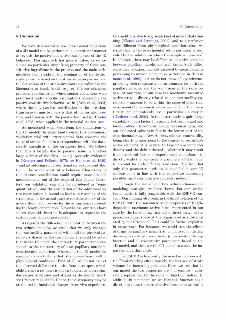
Time-varying elastance. As in (Suga et al, 1973) we

define the instantaneous ventricular elastance E as

E(t) =Pv(t)

V (t)− Vd,

and we represent in Fig.13 the evolution of this quan-

tity in time under constant afterload. More specifically,

we consider two different contractility values, with two

different afterload levels for each of them. We see very

little difference, for each contractility value, between

the curves obtained for the two different afterload lev-

els, as experimentally evidenced in (Suga et al, 1973;

Iribe et al, 2006). Following the classical approach, we

then normalize the elastance by its maximum value in

time – for each simulation separately. When plotting

all these curves together in Fig.13 (c), we obtain very

similar kinetics between the various curves despite the

variations of contractility and afterload, as experimen-

tally observed in (Suga et al, 1973), indeed.

16 M. Caruel et al.

5 Discussion

We have demonstrated how dimensional reductions

of a 3D model can be performed in a consistent manner

as regards the passive and active components of the 3D

behavior. This approach has generic value, as we as-

sumed no particular simplifying property of these con-

stitutive ingredients in the process, and the main tech-

nicalities then reside in the elimination of the hydro-

static pressure based on the stress state properties, and

the derivation of the strain invariants specialized to the

kinematics at hand. In this respect, this extends some

previous approaches in which similar reductions were

performed under specific assumptions concerning the

passive constitutive behavior, as in (Arts et al, 2003)

where the only passive contribution in the directions

transverse to muscle fibers is that of hydrostatic pres-

sure, and likewise with the passive law used in (Hunter

et al, 1998) when applied in the uniaxial tension case.

As mentioned when describing the simulations of

the 1D model, the main limitation of this preliminary

validation trial with experimental data concerns the

range of strains found in correspondence with the data,

clearly unrealistic at the sarcomere level. We believe

that this is largely due to passive tissue in a rather

large vicinity of the clips – as e.g. precisely evidenced

in (Krueger and Pollack, 1975; ter Keurs et al, 1980)

– and introducing some additional series-type contribu-

tion in the overall constitutive behavior. Characterizing

this distinct contribution would require more detailed

measurements, out of the scope of this paper. There-

fore, our validation can only be considered as “semi-

quantitative”, and the elucidation of the additional se-

ries contribution is bound to lead to a rescaling of the

strain scale in the actual passive constitutive law of the

myocardium, and likewise for the n0 function represent-

ing the length-dependence. Nevertheless, our trials have

shown that this function is adequate to represent the

systolic load-dependence effects.

As regards the difference in calibration between the

two reduced models, we recall that we only changed

the contractility parameter, within all the physical pa-

rameters shared by the two models. It should be noted

that in the 1D model the contractility parameter corre-

sponds to the contractility of a rat papillary muscle in

experimental conditions, whereas in the 0D model the

required contractility is that of a human heart wall in

physiological conditions. First of all, we do not expect

the observed difference to arise from inter-species vari-

ability, since a rat heart is known to operate in very sim-

ilar ranges of stresses and strains as the human heart,

see (Pacher et al, 2008). Hence, the discrepancy may be

attributed to functional changes in ex-vivo experimen-

tal conditions, due to e.g. some kind of myocardial stun-

ning (Kloner and Jennings, 2001), and to a perfusion

state different from physiological conditions since we

recall that in the experimental setup perfusion is pro-

vided by the solution in which the sample is immersed.

In addition, there may be differences in active contents

between papillary muscles and wall tissue. Such differ-

ences may be experimentally assessed by measurements

pertaining to myosin contents as performed in (Fitzsi-

mons et al, 1998), but we do not know of any reference

providing such comparative measurements for both the

papillary muscles and the wall tissue in the same or-

gan. At any rate, in our case the maximum measured

active stress – directly related to our contractility pa-

rameter – appears to be within the range of other such

experimentally measured values available in the litera-

ture in similar protocols, see in particular a survey in

(Niederer et al, 2006). In the latter study, a quite large

variability – by a factor 5, typically, between largest and

lowest values – is revealed in such measured data, and

our calibrated value is in fact in the lowest part of the

experimental range. Nevertheless, effective contractility

being clearly proportional to the density of recruitable

active elements, it is natural to take into account this

density and the deficit thereof – whether it may result

from structural factors or experimental conditions – to

directly scale the contractility parameter of the model

to account for such different conditions. The fact that

only this parameter needs to be modified in our 0D

calibration is in line with this conjecture concerning

possible variations in active contents, indeed.

Through the use of our two reduced-dimensional

modeling strategies, we have shown that our cardiac

tissue model is fully compatible with the ESPVR con-

cept. Our findings also confirm the direct relation of the

ESPVR with the sarcomere scale properties of length-

dependent maximum active force, represented in our

case by the function n0 that has a direct image in the

pressure-volume space at the organ level as substanti-

ated by our 0D-model. This could be further exploited

in many ways. For instance, we could test the effects

of drugs on papillary muscles to emulate some cardiac

diseases, accordingly recalibrate (or estimate) the n0-

function and all constitutive parameters based on the

1D-model, and then use the 0D-model to assess the im-

pact on a cardiac cycle.

The ESPVR is frequently discussed in relation with

the Frank-Starling effect, namely, the increase of stroke

volume for increasing preloads. Here, we see that in

our model the two properties are – in essence – accu-

rately represented by the same n0 function, indeed. In

addition, in our model we see that this function has a

direct impact on the rate of active force increase during

Dimensional reductions of a cardiac model for effective validation and calibration 17

contraction. This suggests an additional interpretation

of the Frank-Starling effect, namely, that it primarily

works by increasing this active force build-up rate to

allow a larger strain variation in the same time inter-

val – hence, an increased contraction velocity – for in-

creased end-diastolic strains associated with a higher

preload. This is also fully consistent with the Hill type

force-velocity relations, of course.

Concerning the diastolic load-dependence phenom-

ena, we have proposed a simple modeling ingredient

with a variable following a first-order dynamics that is

used to weigh the activation function, to account for

the variations of unbinding kinetics due to steric effects

in the sarcomere. We have found that this – combined

with the strain rate unbinding term associated with the

parameter α – allows to reproduce quite accurately the

effects measured in the experimental data. However, we

do not claim that the same level of validation has been

achieved here as for systolic effects, since diastolic ef-

fects are much more subtle to characterize based on

experimental data. Furthermore, such effects intervene

in a different manner in actual cardiac physiology, in

which diastole starts with an isovolumic phase, as op-

posed to isometric in the experimental protocol – recall

Fig.5 (a) where only the two orthogonal segments 1-2-3

are explored in both directions instead of a full cycle.

This means that detailed measurements would also be

required to investigate this issue, and possibly to rec-

oncile these effects with the variable elastance theory,

or to identify in which specific context the effects in

question may represent a departure from this theory.

6 Conclusion

We have proposed a generic approach for deriving

reduced-dimensional versions of a 3D heart model. The

1D model was intended to accurately represent the be-

havior of elongated structures such as muscle samples or

myocytes, and we achieved a detailed validation of our

model based on experimental data produced with pap-

illary muscles, in particular concerning length-depend-

ence effects in both systole and diastole. The 0D model

was designed as an approximate representation of a car-

diac cavity – typically the left ventricle – and we have

obtained some most adequate pressure-volume indica-

tors when running simulations of this model with the

parameter values pre-calibrated with the 1D model re-

sults, including when assessing the ESPVR and varying

elastance properties. The 0D model can also readily be

used as a calibration tool for detailed 3D model simula-

tions, or as a boundary condition to an arterial model,

whether to prescribe the inflow, or both fluid and solid

input conditions when appropriate, see (Moireau et al,

2012).

Moreover, our approach of devising several models

within a single hierarchical family sheds some new light

on the relations between the phenomena observed at

different scales and in different contexts. As could be

expected, we find a direct translation of the length-

dependence effect modeled at the sarcomere level and

the load-dependent contraction of a papillary muscle

modeled in our 1D framework. Still more interestingly,

considering concurrently the 1D and 0D models allows

to directly translate at the organ level some findings

obtained at the local level of the sample, and in partic-

ular we have found that the ESPVR curve is a straight-

forward image in the cardiac function of the length-

dependence effects observed at the lower scales. More

generally, this modeling framework could be used as

a tool for predicting the in-vivo manifestations in the

heart of phenomena observed – or induced – in vitro

in various types of experimental testing, such as for as-

sessing the effects of drugs.

Further perspectives include detailed assessments

of a series elasticity contribution in the myocardium

constitutive behavior, based on specific data to be ob-

tained. Moreover, estimation methodologies – also known

as data assimilation, see (Chapelle et al, 2013) and ref-

erences therein – can be expected to be particularly ef-

fective in reduced-dimensional models to automatically

identify model parameters. Indeed, estimation typically

leads to very intensive computations in 3D models, and

convergence in the estimation process is dependent on

the parameter values used as starting points, hence

a preliminary stage of estimation based on a reducedmodel would be of substantial potential benefit.

References

Arts T, Bovendeerd PH, Prinzen FW, Reneman RS

(1991) Relation between left ventricular cavity pres-

sure and volume and systolic fiber stress and strain

in the wall. Biophys J 59(1):93–102

Arts T, Bovendeerd P, Delhaas T, Prinzen F (2003)

Modeling the relation between cardiac pump func-

tion and myofiber mechanics. Journal Of Biomechan-

ics 36(5):731–736

Bathe KJ (1996) Finite Element Procedures. Prentice

Hall, Englewood Cliffs

Bestel J, Clement F, Sorine M (2001) A biomechanical

model of muscle contraction. In: Medical Image Com-

puting and Computer-Assisted Intervention – MIC-

CAI 2001, Springer, pp 1159–1161

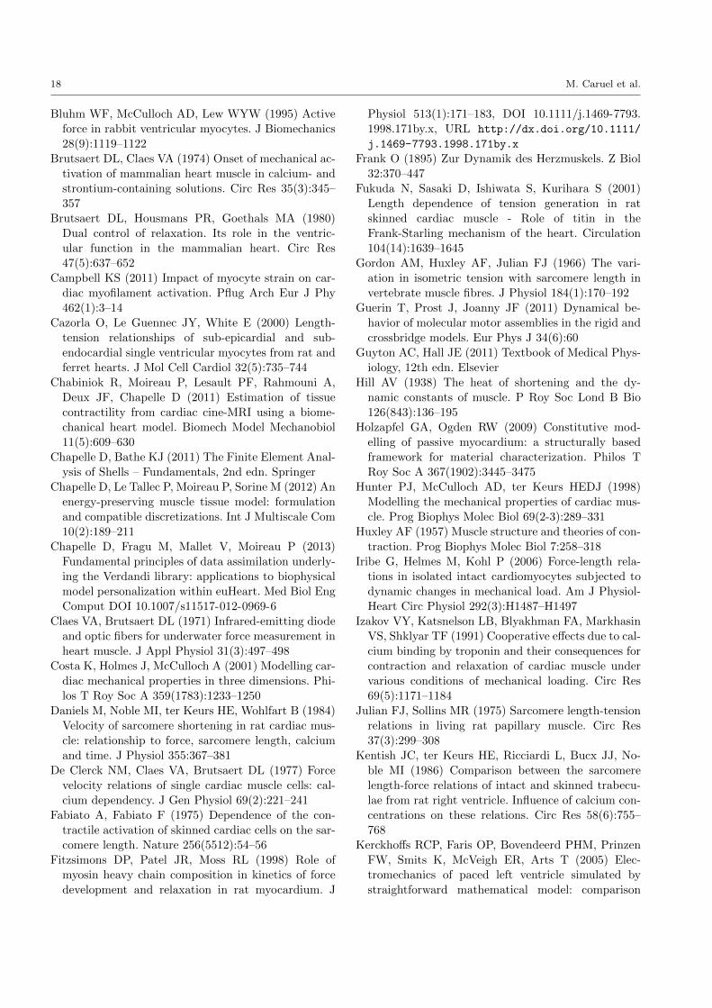
18 M. Caruel et al.

Bluhm WF, McCulloch AD, Lew WYW (1995) Active

force in rabbit ventricular myocytes. J Biomechanics

28(9):1119–1122

Brutsaert DL, Claes VA (1974) Onset of mechanical ac-

tivation of mammalian heart muscle in calcium- and

strontium-containing solutions. Circ Res 35(3):345–

357

Brutsaert DL, Housmans PR, Goethals MA (1980)

Dual control of relaxation. Its role in the ventric-

ular function in the mammalian heart. Circ Res

47(5):637–652

Campbell KS (2011) Impact of myocyte strain on car-

diac myofilament activation. Pflug Arch Eur J Phy

462(1):3–14

Cazorla O, Le Guennec JY, White E (2000) Length-

tension relationships of sub-epicardial and sub-

endocardial single ventricular myocytes from rat and

ferret hearts. J Mol Cell Cardiol 32(5):735–744

Chabiniok R, Moireau P, Lesault PF, Rahmouni A,

Deux JF, Chapelle D (2011) Estimation of tissue

contractility from cardiac cine-MRI using a biome-

chanical heart model. Biomech Model Mechanobiol

11(5):609–630

Chapelle D, Bathe KJ (2011) The Finite Element Anal-

ysis of Shells – Fundamentals, 2nd edn. Springer

Chapelle D, Le Tallec P, Moireau P, Sorine M (2012) An

energy-preserving muscle tissue model: formulation

and compatible discretizations. Int J Multiscale Com

10(2):189–211

Chapelle D, Fragu M, Mallet V, Moireau P (2013)

Fundamental principles of data assimilation underly-

ing the Verdandi library: applications to biophysical

model personalization within euHeart. Med Biol Eng

Comput DOI 10.1007/s11517-012-0969-6

Claes VA, Brutsaert DL (1971) Infrared-emitting diode

and optic fibers for underwater force measurement in

heart muscle. J Appl Physiol 31(3):497–498

Costa K, Holmes J, McCulloch A (2001) Modelling car-

diac mechanical properties in three dimensions. Phi-

los T Roy Soc A 359(1783):1233–1250

Daniels M, Noble MI, ter Keurs HE, Wohlfart B (1984)

Velocity of sarcomere shortening in rat cardiac mus-

cle: relationship to force, sarcomere length, calcium

and time. J Physiol 355:367–381

De Clerck NM, Claes VA, Brutsaert DL (1977) Force

velocity relations of single cardiac muscle cells: cal-

cium dependency. J Gen Physiol 69(2):221–241

Fabiato A, Fabiato F (1975) Dependence of the con-

tractile activation of skinned cardiac cells on the sar-

comere length. Nature 256(5512):54–56

Fitzsimons DP, Patel JR, Moss RL (1998) Role of

myosin heavy chain composition in kinetics of force

development and relaxation in rat myocardium. J

Physiol 513(1):171–183, DOI 10.1111/j.1469-7793.

1998.171by.x, URL http://dx.doi.org/10.1111/

j.1469-7793.1998.171by.x

Frank O (1895) Zur Dynamik des Herzmuskels. Z Biol

32:370–447

Fukuda N, Sasaki D, Ishiwata S, Kurihara S (2001)

Length dependence of tension generation in rat

skinned cardiac muscle - Role of titin in the

Frank-Starling mechanism of the heart. Circulation

104(14):1639–1645

Gordon AM, Huxley AF, Julian FJ (1966) The vari-

ation in isometric tension with sarcomere length in

vertebrate muscle fibres. J Physiol 184(1):170–192

Guerin T, Prost J, Joanny JF (2011) Dynamical be-

havior of molecular motor assemblies in the rigid and

crossbridge models. Eur Phys J 34(6):60

Guyton AC, Hall JE (2011) Textbook of Medical Phys-

iology, 12th edn. Elsevier

Hill AV (1938) The heat of shortening and the dy-

namic constants of muscle. P Roy Soc Lond B Bio

126(843):136–195

Holzapfel GA, Ogden RW (2009) Constitutive mod-

elling of passive myocardium: a structurally based

framework for material characterization. Philos T

Roy Soc A 367(1902):3445–3475

Hunter PJ, McCulloch AD, ter Keurs HEDJ (1998)

Modelling the mechanical properties of cardiac mus-

cle. Prog Biophys Molec Biol 69(2-3):289–331

Huxley AF (1957) Muscle structure and theories of con-

traction. Prog Biophys Molec Biol 7:258–318

Iribe G, Helmes M, Kohl P (2006) Force-length rela-

tions in isolated intact cardiomyocytes subjected to

dynamic changes in mechanical load. Am J Physiol-

Heart Circ Physiol 292(3):H1487–H1497

Izakov VY, Katsnelson LB, Blyakhman FA, Markhasin

VS, Shklyar TF (1991) Cooperative effects due to cal-

cium binding by troponin and their consequences for

contraction and relaxation of cardiac muscle under

various conditions of mechanical loading. Circ Res

69(5):1171–1184

Julian FJ, Sollins MR (1975) Sarcomere length-tension

relations in living rat papillary muscle. Circ Res

37(3):299–308

Kentish JC, ter Keurs HE, Ricciardi L, Bucx JJ, No-

ble MI (1986) Comparison between the sarcomere

length-force relations of intact and skinned trabecu-

lae from rat right ventricle. Influence of calcium con-

centrations on these relations. Circ Res 58(6):755–

768

Kerckhoffs RCP, Faris OP, Bovendeerd PHM, Prinzen

FW, Smits K, McVeigh ER, Arts T (2005) Elec-

tromechanics of paced left ventricle simulated by

straightforward mathematical model: comparison

Dimensional reductions of a cardiac model for effective validation and calibration 19

with experiments. Am J Physiol Heart Circ Physiol

289(5):H1889–97

ter Keurs HE, Rijnsburger WH, van Heuningen R,

Nagelsmit MJ (1980) Tension development and sar-

comere length in rat cardiac trabeculae. Evidence of

length-dependent activation. Circ Res 46(5):703–714

Kloner R, Jennings R (2001) Consequences of brief is-

chemia: Stunning, preconditioning, and their clinical

implications, part 1. Circulation 24(104):2981–2989

Koiter W (1965) On the nonlinear theory of thin elastic

shells. Proc Kon Ned Akad Wetensch B69:1–54

Krueger JW, Pollack GH (1975) Myocardial sarcom-

ere dynamics during isometric contraction. J Physiol

251(3):627–643

Lecarpentier YC, Chuck LH, Housmans PR, De Clerck

NM, Brutsaert DL (1979) Nature of load dependence

of relaxation in cardiac muscle. Am J Physiol-Heart

Circ Physiol 237(4):H455–H460

Linari M, Bottinelli R, Pellegrino M, Reconditi M, Reg-

giani C, Lombardi V (2004) The mechanism of the

force response to stretch in human skinned muscle fi-

bres with different myosin isoforms (vol, 554, pg 335,

2004). J Physiol 555:851

Linari M, Caremani M, Piperio C, Brandt P, Lombardi

V (2007) Stiffness and fraction of myosin motors re-

sponsible for active force in permeabilized muscle

fibers from rabbit psoas. Biophys J 92:2476–2490

Linari M, Piazzesi G, Lombardi V (2009) The ef-

fect of myofilament compliance on kinetics of force

generation by myosin motors in muscle. Biophys J

96(2):583–592

Linari M, Caremani M, Lombardi V (2010) A kinetic

model that explains the effect of inorganic phosphate

on the mechanics and energetics of isometric contrac-

tion of fast skeletal muscle. P Roy Soc Lond B Bio

277(270):19–27

Linke W, Fernandez J (2002) Cardiac titin: molecular

basis of elasticity and cellular contribution to elastic

and viscous stiffness components in myocardium. J

Muscle Res Cell Motil 23(5-6):483–497

Linke WA, Popov VI, Pollack GH (1994) Passive and

active tension in single cardiac myofibrils. Biophys J

67(2):782–792

Lumens J, Delhaas T, Kirn B, Arts T (2009) Three-

wall segment (TriSeg) model describing mechanics

and hemodynamics of ventricular interaction. Ann

Biomed Eng 37(11):2234–2255

Lymn R, Taylor E (1971) Mechanism of adenosine

triphosphate hydrolysis by actomyosin. Biochemistry

10(25):4617–&Moireau P, Chapelle D, Le Tallec P (2008) Joint state

and parameter estimation for distributed mechanical

systems. Computer Methods in Applied Mechanics

and Engineering 197:659–677

Moireau P, Xiao N, Astorino M, Figueroa CA, Chapelle

D, Taylor C A, Gerbeau JF (2012) External tissue

support and fluid-structure simulation in blood flows.

Biomech Model Mechanobiol 11(1-2):1–18, DOI 10.

1007/s10237-011-0289-z, URL http://hal.inria.

fr/hal-00701801

Moss RL, Fitzsimons DP (2002) Frank-Starling Rela-

tionship - Long on importance, short on mechanism.

Circ Res 90(1):11–13

Nash M, Hunter P (2000) Computational mechanics of

the heart - From tissue structure to ventricular func-

tion. J Elasticity 61(1-3):113–141

Niederer SA, Smith NP (2009) The Role of the

Frank–Starling Law in the Transduction of Cellu-

lar Work to Whole Organ Pump Function: A Com-

putational Modeling Analysis. PLoS Comput Biol

5(4):e1000,371

Niederer SA, Hunter PJ, Smith NP (2006) A quantita-

tive analysis of cardiac myocyte relaxation: A simu-

lation study. Biophys J 90(5):1697–1722

Pacher P, Nagayama T, Mukhopadhyay P, Batkai S,

Kass DA (2008) Measurement of cardiac function us-

ing pressure-volume conductance catheter technique

in mice and rats. Nature Protocols 3(9):1422–1434

Panerai RB (1980) A model of cardiac muscle mechan-

ics and energetics. J Biomechanics 13:929–940

Parikh SS, Zou SZ, Tung L (1993) Contraction and re-

laxation of isolated cardiac myocytes of the frog un-

der varying mechanical loads. Circ Res 72(2):297–311

Peskin CS (1975) Mathematical Aspects of Heart Phys-

iology. Courant Institute of Mathematical Sciences

Piazzesi G, Reconditi M, Linari M, Lucii L, Bianco P,

Brunello E, Decostre V, Stewart A, Gore DB, Irving

TC, Irving M, Lombardi V (2007) Skeletal muscle

performance determined by modulation of number

of myosin motors rather than motor force or stroke

size. Cell 131(4):784–795

Sachse FB (2004) Computational Cardiology: Model-

ing of Anatomy, Electrophysiology, and Mechanics.

Springer

Sainte-Marie J, Chapelle D, Cimrman R, Sorine M

(2006) Modeling and estimation of the cardiac elec-

tromechanical activity. Comput Struct 84(28):1743–

1759

Schmid H, O’Callaghan P, Nash MP, Lin W, LeGrice

IJ, Smaill BH, Young AA, Hunter PJ (2008) Myocar-

dial material parameter estimation. Biomech Model

Mechanobiol 7(3):161–173

Senzaki H, Chen CH, Kass DA (1996) Single-beat es-

timation of end-systolic pressure-volume relation in

humans: a new method with the potential for nonin-

vasive application. Circulation 94:2497–2506

20 M. Caruel et al.

Shiels HA, White E (2008) The Frank–Starling mech-

anism in vertebrate cardiac myocytes. J Exp Biol

211(13):2005–2013

Smith N, et al (2011) euHeart: personalized and inte-

grated cardiac care using patient-specific cardiovas-

cular modelling. Interface Focus 1(3):349–364

Sonnenblick EH (1962) Force-velocity relations in mam-

malian heart muscle. Am J Physiol 202(5):931–939

Starling EH (1918) The Linacre Lecture on the Law

of the Heart Given at Cambridge, 1915. Nature

101(2525):43–43

Suga H, Sagawa K, Shoukas AA (1973) Load indepen-

dence of the instantaneous pressure-volume ratio of

the canine left ventricle and effects of epinephrine and

heart rate on the ratio. Circ Res 32(3):314–322

Takeuchi M, Igarashi Y, Tomimoto S, Odake M,

Hayashi T, Tsukamoto T, Hata K, Takaoka H,

Fukuzaki H (1991) Single-beat estimation of the slope

of the end-systolic pressure-volume relation in the hu-

man left ventricle. Circulation 83:202–212

de Tombe PP, ter Keurs HE (1990) Force and velocity

of sarcomere shortening in trabeculae from rat heart.

Effects of temperature. Circ Res 66(5):1239–1254

Tortora GJ, Derrikson B (2009) Principles of Anatomy

and Physiology, 12th edn. John Wiley & Sons, Inc

Trayanova NA, Rice JJ (2011) Cardiac electromechan-

ical models: from cell to organ. Front Physiol 2:43

Weiwad WK, Linke WA, Wussling MH (2000) Sar-

comere length-tension relationship of rat cardiac my-

ocytes at lengths greater than optimum. J Mol Cell

Cardiol 32(2):247–259

Wong AYK (1972) Mechanics of cardiac muscle, based

on Huxley’s model: Simulation of active state and

force-velocity relation. J Biomechanics 5(1):107–117

Zahalak GI, Ma S (1990) Muscle activation and con-

traction: constitutive relations based directly on

cross-bridge kinetics. J Biomech Eng 112(1):52–62