dimers and orthogonal polynomials: connections...
TRANSCRIPT

Dimers and orthogonal polynomials:connections with random matrices
Extended lecture notes of the minicourse at IHP
Patrik L. Ferrari
Bonn [email protected]
Version of December 14, 2009
Abstract
In these lecture notes we present some connections between ran-dom matrices, the asymmetric exclusion process, random tilings.These three apparently unrelated objects have (sometimes) a similarmathematical structure, an interlacing structure, and the correlationfunctions are given in terms of a kernel. In the basic examples, thekernel is expressed in terms of orthogonal polynomials.
Contents
1 Gaussian Unitary Ensemble of random matrices (GUE) 21.1 The Gaussian Ensembles of random matrices . . . . . . . . . . 21.2 Eigenvalues’ distribution . . . . . . . . . . . . . . . . . . . . . 41.3 Orthogonal polynomials . . . . . . . . . . . . . . . . . . . . . 51.4 Correlation functions of GUE . . . . . . . . . . . . . . . . . . 61.5 GUE kernel and Hermite polynomials . . . . . . . . . . . . . . 81.6 Distribution of the largest eigenvalue: gap probability . . . . . 91.7 Correlation functions of GUE minors: interlacing structure . . 10
1
2 Totally Asymmetric Simple Exclusion Process (TASEP) 142.1 Continuous time TASEP: interlacing structure . . . . . . . . . 142.2 Correlation functions for step initial conditions: Charlier poly-
nomials . . . . . . . . . . . . . . . . . . . . . . . . . . . . . . 182.3 Discrete time TASEP . . . . . . . . . . . . . . . . . . . . . . . 21
3 2 + 1 dynamics: connection to random tilings and randommatrices 243.1 2 + 1 dynamics for continuous time TASEP . . . . . . . . . . 253.2 Interface growth interpretation . . . . . . . . . . . . . . . . . . 273.3 Random tilings interpretation . . . . . . . . . . . . . . . . . . 273.4 Diffusion scaling and relation with GUE minors . . . . . . . . 283.5 Shuffling algorithm and discrete time TASEP . . . . . . . . . 29
A Further references 31
B Christoffel-Darboux formula 33
C Proof of Proposition 6 34
1 Gaussian Unitary Ensemble of random ma-
trices (GUE)
Initially studied by statisticians in the 20’s-30’s, random matrices are thenintroduced in nuclear physics in the 60’s to describe the energy levels distri-bution of heavy nuclei. The reader interested in a short discussion on randommatrices in physics can read [37], in mathematics [43], and a good referencefor a more extended analysis is [38].
1.1 The Gaussian Ensembles of random matrices
The Gaussian ensembles of random matrices have been introduced by physi-cists (Dyson, Wigner, ...) in the sixties to model statistical properties of theresonance spectrum of heavy nuclei. The energy levels of a quantum systemare the eigenvalues of an Hamiltonian. For heavy nuclei some properties ofthe spectrum, like eigenvalues’ spacing statistics, seemed to have some reg-ularity (e.g., repulsions) common for all heavy nuclei. In other words there
2

was some universal behavior. If such a universal behavior exists, then it hasto be the same as the behavior of choosing a random Hamiltonian. Moreover,since the heavy nuclei have a lot of bound stated (i.e., where the eigenvalueswith normalizable eigenfunctions), the idea is to approximate it by a largematrix with random entries.
Even assuming the entries of the matrix random, to have a chance todescribe the physical properties of heavy atoms, the matrices need to satisfythe intrinsic symmetries of the systems:
1. a real symmetric matrix can, a priori, describe a system with time rever-sal symmetry and rotation invariance or integer magnetic momentum,
2. a real quaternionic matrix (i.e., the basis are the Pauli matrices) can beused for time reversal symmetry and half-integer magnetic momentum,
3. a complex hermitian matrix can describe a system which is not timereversal invariant (e.g., with external magnetic field).
We now first focus on the complex hermitian matrices case, since it is theone we are going to discuss later on.
Definition 1. The Gaussian Unitary Ensemble (GUE) of random ma-trices is a probability measure P on the set of N × N complex hermitianmatrices, with density
P(dH) =1
ZNexp
(− β
4NTr(H2)
)dH, with β = 2, (1)
where dH =∏N
i=1 dHi,i
∏1≤i<j≤N dRe(Hi,j)dIm(Hi,j) is the reference mea-
sure, and ZN is the normalization constant.
The meaning of β = 2 will be clear once we consider the induced measureon the eigenvalues.
Concerning the meaning of GUE, notice that the measure (1) is invariantover the unitary transformations and has a Gaussian form. The invarianceover the unitary transformations is physically motivated, because the physicalsystem does not depend on the choice of basis used to describe it. Indeed, byimposing that the measure P is (a) invariant under the change of basis (in thepresent case, invariant under the action of the group of symmetry U(N)) and
3

a = 1/2N a = 1 a = N
Largest eigenvalue 2N +O(N1/3)√2N +O(N−1/6)
√2 +O(N−2/3)
Eigenvalues density O(1) O(N1/2) O(N)
Table 1: Typical scaling for the Gaussian Unitary Ensemble
(b) the entries of the matrices as independent random variables (of course,up to the required symmetry), then one gets the family of measures
exp(−aTr(H2) + bTr(H) + c
), a > 0, b, c ∈ R. (2)
The value of (c) is determined by the normalization requirement, while byan appropriate shift of the zeros of the energy (i.e., H → H − E for somegiven E), we can set b = 0. The energy shift is irrelevant from the physicspoint of view, because by the first principle of thermodynamics the energyof a system is an extensive observable defined up to a constant. The value ofa remains free to be chosen. Different choices can be easily compared sinceare just a change of scale of each others. In the literature there are mainlythree typical choices, see Table 1, each one with its own reason.
Another way to obtain (1) is to take the random variables, Hi,i ∼ N (0, N)for i = 1, . . . , N , and Re(Hi,j) ∼ N (0, N/2), Im(Hi,j) ∼ N (0, N/2) for1 ≤ i < j ≤ N as independent random variables.
For the class of real symmetric (resp. quaternionic), one defines theGaussian Orthogonal Ensemble (GOE) (resp. Gaussian Symplectic Ensemble(GSE)) as in Definition 1 but with β = 1 (resp. β = 4) and, of course, thereference measure is now the product Lebesgue measure over the independententries of the matrices.
1.2 Eigenvalues’ distribution
For the Gaussian ensembles of random matrices, one quantity of interest arethe eigenvalues, which are independent of the choice of basis. By integratingout the angular variables one obtains the following result. Denote by PGUE(λ)the probability density of eigenvalues at λ ∈ R
N .
4
Proposition 2. Let λ1, λ2, . . . , λN ∈ R denote the N eigenvalues of a randommatrix H with measure (1). Then, the joint distribution of eigenvalues isgiven by
PGUE(λ) =1
ZN|∆N(λ)|β
N∏
i=1
exp
(− β
4Nλ2i
), with β = 2, (3)
∆N(λ) :=∏
1≤i<j≤N(λj − λi) is the Vandermonde determinant, and ZN is anormalization constant.
The following identity shows why ∆N is called a determinant
∆N (λ) = det[λj−1i
]1≤i,j≤N
. (4)
Notice that PGUE(# e.v. ∈ [x, x + dx]) ∼ (dx)2, so that the probability ofhaving double points is zero: it is a simple point process.
For GOE (resp. GSE) the joint distributions of eigenvalues has theform (3) but with β = 1 (resp. β = 4) instead.
1.3 Orthogonal polynomials
Here we describe orthogonal polynomials on R, but the formulas can beeasily adapted for polynomials on Z by replacing the Lebesgue measure bythe counting measure and integrals by sums.
Definition 3. Given a weight ω : R 7→ R+, the orthogonal polynomials
{qk(x), k ≥ 0} are defined by the following two conditions,
1. qk(x) is a polynomial of degree k with qk(x) = ukxk + . . ., uk > 0,
2. they satisfy the orthonormality condition,
〈qk, ql〉ω :=
∫
R
ω(x)qk(x)ql(x)dx = δk,l. (5)
Remark 4. There are other normalizations which are often used, like inthe Askey Scheme of hypergeometric orthogonal polynomials [36]. Some-times, the polynomials are taken to be monic, i.e., uk = 1 and the or-thonormality condition has then to be replaced by an orthogonality condi-tion
∫Rω(x)qk(x)ql(x)dx = ckδk,l. Of course qk(x) = qk(x)/uk and ck = 1/u2k.
Sometimes, the polynomials are neither orthonormal (like in Definition 3)nor monic, like the standard Hermite polynomials that we will encounter,and are given by derivatives of a given (generating) function.
5

A useful formula for sums of orthogonal polynomials is the Christoffel-Darboux formula:
N−1∑
k=0
qk(x)qk(y) =
uN−1
uN
qN (x)qN−1(y)− qN−1(x)qN (y)
x− y, for x 6= y,
uN−1
uN(q′N (x)qN−1(x)− q′N−1(x)qN (x)), for x = y.
(6)This formula is proven by employing the following three term relation
qn(x) = (Anx+Bn)qn−1(x)− Cnqn−2(x), (7)
with An > 0, Bn, Cn > 0 some constants. See Appendix B for details of thederivation. For polynomials as in Definition 3, it holds An = un/un−1 andCn = An/An−1 = unun−2/u
2n−1.
1.4 Correlation functions of GUE
Now we restrict the point of view to the GUE ensemble and discuss thederivation of the correlation functions for the GUE eigenvalues’ point process.
Let the reference measure be Lebesgue. Then, the n-point correlationfunction, ρ
(n)GUE(x1, . . . , xn) is the probability density of finding an eigenvalue
at each of the xk, k = 1, . . . , n. PGUE defined in (3) is symmetric in RN ,
which directly implies the following result.
Lemma 5. The n-point correlation function for GUE eigenvalues is givenby
ρ(n)GUE(x1, . . . , xn) =
N !
(N − n)!
∫
RN−n
PGUE(x1, . . . , xN)dxn+1 . . . dxN (8)
for n = 1, . . . , N and ρ(n)GUE(x1, . . . , xn) = 0 for n > N .
It is important to notice that it is not fixed which eigenvalue is at whichposition. In particular, we have
ρ(1)GUE(x) = eigenvalues’ density at x =⇒
∫
R
ρ(1)GUE(x)dx = N. (9)
More generally,∫
Rn
ρ(n)GUE(x1, . . . , xn)dx1 . . .dxn =
N !
(N − n)!. (10)
6

Our next goal is to do the integration in (8). For that purpose, wewill use Hermite orthogonal polynomials. For any family of polynomials{qk, k = 0, . . . , N − 1}, where qk has degree k, by multi-linearity of the de-terminant, it holds
∆N(λ) = det[λj−1i ]1≤i,j≤N = const× det[qj−1(λi)]1≤i,j≤N . (11)
Therefore, setting ω(x) := exp(−x2/2N), we have
PGUE(λ1, . . . , λN)
= const× det[qk−1(λi)]1≤i,k≤N det[qk−1(λj)]1≤k,j≤N
N∏
i=1
ω(λi)
= const× det
[N∑
k=1
qk−1(λi)qk−1(λj)
]
1≤i,j≤N
N∏
i=1
ω(λi).
(12)
Notice that until this point, the polynomials q’s do not have to be orthogonal.However, if we choose the polynomials orthogonal with respect to the weightω, then the integrations in (8) becomes particularly simple and nice.
Proposition 6. Let qk be orthogonal polynomials with respect to the weightω(x) = exp(−x2/2N). Then,
ρ(n)GUE(x1, . . . , xn) = det
[KGUE
N (xi, xj)]1≤i,j≤n
, (13)
where
KGUEN (x, y) =
√ω(x)
√ω(y)
N−1∑
k=0
qk(x)qk(y). (14)
The proof of Proposition 6 can be found in Appendix C. What we needto do is integrate out the N − n variables one after the other and see thatthe determinant keeps the same entries but becomes smaller. For that weuse the following two identities
∫
R
KGUEN (x, x)dx = N,
∫
R
KGUEN (x, z)KGUE
N (z, y)dz = KGUEN (x, y).
(15)
7

It is at this point that the particular choice of orthogonal polynomials isessential. Indeed, (15) hold for the kernel defined by the r.h.s. of (14) preciselywhen qk(x) are taken to be orthogonal to ω(x).
The particular form of correlation functions (13) appears also in othersystems.
Definition 7. A point process (i.e., a random point measure) is called de-
terminantal if its n-point correlation function has the form
ρ(n)(x1, . . . , xn) = det[K(xi, xj)]1≤i,j≤n (16)
for some (measurable) function K : R2 → R, called the kernel of the deter-minantal point process.
One might ask when a measure defines a determinantal point process. Asufficient condition is the following (see Proposition 2.2 of [4]).
Theorem 8. Consider a probability measure on RN of the form
1
ZNdet[φi(xj)]1≤i,j≤N det[ψi(xj)]1≤i,j≤N
N∏
i=1
ω(xi)dxi, (17)
with the normalization ZN 6= 0. Then (17) defines a determinantal pointprocess with kernel
KN(x, y) =N∑
i,j=1
ψi(x)[A−1]i,jφj(y), (18)
where A = [Ai,j ]1≤i,j≤N ,
Ai,j = 〈φi, ψj〉ω =
∫
R
ω(z)φi(z)ψj(z)dz. (19)
1.5 GUE kernel and Hermite polynomials
Finally, let us give an explicit formula for the kernel KN . The standardHermite polynomials, {Hn, n ≥ 0}, are defined by
Hk(y) = (−1)key2 dk
dyke−y2 . (20)
8
They satisfy ∫
R
e−y2Hk(y)Hl(y)dy =√π2kk!δk,l, (21)
with Hk(y) = 2kyk + . . ., and also
d
dy
(e−y2Hn(y)
)= −e−y2Hn+1(y) ⇒
∫ x
−∞e−y2Hn+1(y)dy = −e−x2
Hn(x).
(22)By the change of variable y = x/
√2N and a simple computation, one
shows that
qk(x) =1
4√2πN
1√2kk!
Hk
(x√2N
)(23)
are orthogonal polynomials with respect to ω(x) = exp(−x2/2N), and thatuk = (2πN)−1/4k!−1/2N−k/2. Then, Christoffel-Darboux formula (6) gives
KGUEN (x, y) =
qN(x)qN−1(y)− qN−1(x)qN(y)
x− yNe−(x2+y2)/4N , for x 6= y,
(q′N(x)qN−1(x)− q′N−1(x)qN (x))Ne−(x2+y2)/4N , for x = y.
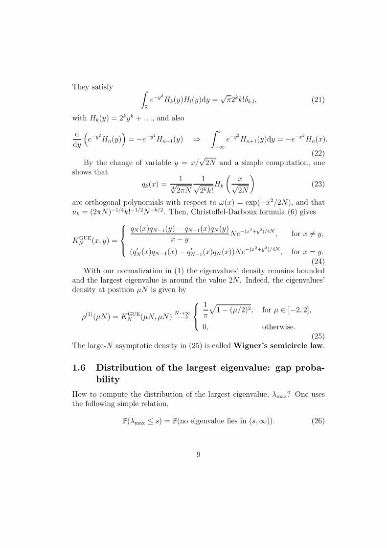
(24)With our normalization in (1) the eigenvalues’ density remains bounded
and the largest eigenvalue is around the value 2N . Indeed, the eigenvalues’density at position µN is given by
ρ(1)(µN) = KGUEN (µN, µN)
N→∞−→
1
π
√1− (µ/2)2, for µ ∈ [−2, 2],
0, otherwise.(25)
The large-N asymptotic density in (25) is called Wigner’s semicircle law.
1.6 Distribution of the largest eigenvalue: gap proba-bility
How to compute the distribution of the largest eigenvalue, λmax? One usesthe following simple relation,
P(λmax ≤ s) = P(no eigenvalue lies in (s,∞)). (26)
9

This is a special case of gap probability, i.e., probability that in a Borelset B there are no eigenvalues. The gap probabilities are expressed in termsof n-point correlation functions as follows.
P(no eigenvalue lies in B) = E
(∏
i
(1− 1B(λi))
)
=∑
n≥0
(−1)nE
( ∑
i1<...<in
n∏
k=1
1B(λik)
)sym=
∑
n≥0
(−1)n
n!E
( ∑
i1,...,inall different
n∏
k=1
1B(λik)
)
=∑
n≥0
(−1)n
n!
∫
Bn
ρ(n)(x1, . . . , xn)dx1 . . .dxn,
(27)where 1B(x) = 1 if x ∈ B and 1B(x) = 0 if x 6∈ B. The last step holds forsimple point processes.
For a determinantal point process, like the GUE eigenvalues, the r.h.s. of(27) is the Fredholm series expansion of the Fredholm determinant:
P(λmax ≤ s) =
∞∑
n=0
(−1)n
n!
∫
(s,∞)ndet[KGUE
N (xi, xj)]1≤i,j≤ndx1 . . .dxn
≡ det(1−KGUEN )L2((s,∞),dx).
(28)
In our case the sums over n are actually finite (for n > N the terms areequal to zero, since the kernel KN has rank N), but we preferred to keep theformulation of the general case.
1.7 Correlation functions of GUE minors: interlacing
structure
Interestingly, the determinantal structure still holds in the enlarged settingof eigenvalues of minors.
Consider a N × N GUE random matrix H and denote by λN1 , . . . , λNN
its eigenvalues. Then, denote by Hm the m × m minor of the matrix Hwhere the last N − m rows and columns have been deleted. Denote byλm1 , . . . , λ
mm the eigenvalues of Hm. In [26, 33] the correlation functions of
{λmk , 1 ≤ k ≤ m ≤ N} are determined. It turns out that also in that casethe correlation functions are determinantal (on {1, . . . , N} × R).
10

λ11
λ21 λ22
λ31 λ32 λ33
λ41 λ42 λ43 λ44
n
R1
2
3
4
Figure 1: Illustration of the interlacing structure of the GUE minors’ eigen-values.
Let us order the eigenvalues for each minors as follows,λm1 ≤ λm2 ≤ . . . ≤ λmm. Then, the GUE minor measure can be writtenas, see e.g. [26],
const×(N−1∏
m=1
det[φ(λmi , λm+1j )]1≤i,j≤m+1
)det[ΨN
N−i(λNj )]1≤i,j≤N (29)
where λmm+1 ≡ virt are virtual variables, φ(x, y) = 1(x > y), φ(virt, y) = 1,and
ΨNN−k(x) =
(−1)N−k
(2N)(N−k)/2e−x2/2NHN−k(x/
√2N). (30)
The eigenvalues of the minors have a nice structure which appears in otherproblems too, see next sections. (29) is non-zero if and only if the eigenvaluessatisfy the following interlacing structure, see Figure 1 for an illustration,
λm+11 < λm1 ≤ λm+1
2 < λm2 ≤ . . . < λmm ≤ λm+1m+1, (31)
for m = 1, . . . , N − 1. Indeed,
det[φ(λmi , λm+1j )]1≤i,j≤m+1 =
{1, if (31) is satisfied,0, otherwise.
(32)
One might have seen that some inequalities were replaced by strict inequal-ities, but this is irrelevant since the events with λnk = λn+1
k have probabilityzero.
Let us define,Ψn
n−k(x) := (φ ∗Ψn+1n+1−k)(x). (33)
11
Then, a straightforward consequence of (22), is
Ψnn−k(x) =
(−1)n−k
(2N)(n−k)/2e−x2/2NHn−k(x/
√2N) (34)
for 1 ≤ k ≤ n. Moreover, it is easy to verify that
∫
Rn(n−1)/2
∏
1≤k≤m≤n−1
dλmk
n−1∏
m=1
det[φ(λmi , λm+1j )]1≤i,j≤m+1 = ∆n(λ
n1 , . . . , λ
nn).
(35)To get an explicit expression of the kernel (see Theorem 10 below), we needto find functions {Φn
n−k, k = 1, . . . , n} orthogonal, with respect to the weightω = 1, to the functions {Ψn
n−j, j = 1, . . . , n}, and such that
span{Φn0 (x), . . . ,Φ
nn−1(x)} = span{1, x, . . . , xn−1}. (36)
We find
Φnn−j(x) =
(−1)n−j
√2π(n− j)!
(N
2
)(n−j)/2
Hn−j(x/√2N). (37)
A measure of the form (29) has determinantal correlations [9]. The differ-ence with the above case is that the correlation functions are determinantalon {1, . . . , N} × R instead of R. This means the following. The probabilitydensity of finding an eigenvalue of Hni
at position xi, for i = 1, . . . , n, is givenby
ρ(n)((ni, xi), 1 ≤ i ≤ n) = det[KGUE
N (ni, xi;nj , xj)]1≤i,j≤n
. (38)
The kernel KGUEN is computed applying the general Theorem 10 which we
report below, but first we give the solution.
Proposition 9. The correlation functions of the GUE minors are determi-nantal with kernel given by
KGUEN (n1, x1;n2, x2) = −(φ∗(n2−n1))(x1, x2)1[n1<n2]+
n2∑
k=1
Ψn1n1−k(x1)Φ
n2n2−k(x2),
(39)with φ∗(n2−n1) the convolution of φ with itself n2 − n1 times, namely, forn2 > n1,
(φ∗(n2−n1))(x1, x2) =(x2 − x1)
n2−n1−1
(n2 − n1 − 1)!1[x2−x1≥0]. (40)
12

The following result is generalization of Theorem 8.
Theorem 10. Assume we have a measure on {xni , 1 ≤ i ≤ n ≤ N} given inthe form,
1
ZN
(N−1∏
n=1
det[φn(xni , x
n+1j )]1≤i,j≤n+1
)det[ΨN
N−i(xNj )]1≤i,j≤N , (41)
where xnn+1 are some “virtual” variables and ZN is a normalization constant.If ZN 6= 0, then the correlation functions are determinantal.
To write down the kernel we need to introduce some notations. Define
φ(n1,n2)(x, y) =
{(φn1 ∗ · · · ∗ φn2−1)(x, y), n1 < n2,0, n1 ≥ n2,
(42)
where (a ∗ b)(x, y) =∫Ra(x, z)b(z, y)dz, and, for 1 ≤ n < N ,
Ψnn−j(x) := (φ(n,N) ∗ΨN
N−j)(y), j = 1, 2, . . . , N. (43)
Set φ0(x01, x) = 1. Then the functions
{(φ0 ∗ φ(1,n))(x01, x), . . . , (φn−2 ∗ φ(n−1,n))(xn−2n−1, x), φn−1(x
n−1n , x)} (44)
are linearly independent and generate the n-dimensional space Vn. Define aset of functions {Φn
j (x), j = 0, . . . , n− 1} spanning Vn defined by the orthog-onality relations ∫
R
Φni (x)Ψ
nj (x)dx = δi,j (45)
for 0 ≤ i, j ≤ n− 1.Under Assumption (A): φn(x
nn+1, x) = cnΦ
(n+1)0 (x), for some cn 6= 0,
n = 1, . . . , N − 1, the kernel takes the simple form
K(n1, x1;n2, x2) = −φ(n1,n2)(x1, x2) +
n2∑
k=1
Ψn1n1−k(x1)Φ
n2n2−k(x2). (46)
Remark 11. Without Assumption (A), the correlations functions are stilldeterminantal but the formula is modified as follows. Let M be the N ×Ndimensional matrix defined by [M ]i,j = (φi−1 ∗ φ(i,N) ∗ΨN
N−j)(xi−1i ). Then
K(n1, x1;n2, x2) (47)
= −φ(n1,n2)(x1, x2) +N∑
k=1
Ψn1n1−k(x1)
n2∑
l=1
[M−1]k,l(φl−1 ∗ φ(l,n2))(xl−1l , x2).
13

The “virtual variables” are just there to write the formula in a simpler way,but they do not represent real variables. This can be seen for example inAssumption (A), where the r.h.s. does not depend on xnn+1. Theorem 10 isproven by using the framework of [17].
In the case of the measure (29), the n-dimensional space Vn is spannedby {1, x, . . . , xn−1}, so Φn
k have to be polynomials of degree k, compare with(37).
2 Totally Asymmetric Simple Exclusion Pro-
cess (TASEP)
2.1 Continuous time TASEP: interlacing structure
The totally asymmetric simple exclusion process (TASEP) is one of the sim-plest interacting stochastic particle systems. It consists of particles on thelattice of integers, Z, with at most one particle at each site (exclusion prin-ciple). The dynamics in continuous time is as follows. Particles jump on theneighboring right site with rate 1 provided that the site is empty. This meansthat jumps are independent of each other and take place after an exponentialwaiting time with mean 1, which is counted from the time instant when theright neighbor site is empty.
Here we consider all particles with equal rate 1. However, the frameworkwhich we explain below, can be generalized to particle-dependent rates andalso particles can jump on both directions (but with different rules, it isnot the partially asymmetric case): by jumping on their right, particles canbe blocked, while on the left if a site is occupied, then it is pushed by thejumping particle. This generalization, called PushASEP, together with apartial extension to space-time correlations is the content of our paper [6].
On the macroscopic level the particle density, u(x, t), evolves deterministi-cally according to the Burgers equation ∂tu+∂x(u(1−u)) = 0 [49]. Thereforea natural question is to focus on fluctuation properties, which exhibit ratherunexpected features. The asymptotic results can be found in the literature,see Appendix A. Here we focus on a method which can be used to analyzethe joint distributions of particles’ positions. This method is based on a in-terlacing structure first discovered by Sasamoto in [51], later extended andgeneralized in a series of papers, starting with [9]. We explain the key steps
14

following the notations of [9], where the details of the proofs can be found.Consider the TASEP with N particles starting at time t = 0 at positions
yN < . . . < y2 < y1. The first step is to obtain the probability that at time tthese particles are at positions xN < . . . < x2 < x1, which we denote by
G(x1, . . . , xN ; t) = P((xN , . . . , x1; t)|(yN , . . . , y1; 0)). (48)
This function has firstly been determined using Bethe-Ansatz method [53]. Aposteriori, the result can be checked directly by writing the master equation.
Lemma 12. The transition probability is given by
G(x1, . . . , xN ; t) = det(Fi−j(xN+1−i − yN+1−j , t))1≤i,j≤N (49)
with
Fn(x, t) =(−1)n
2πi
∮
Γ0,1
dw
w
(1− w)−n
wx−net(w−1), (50)
where Γ0,1 is any simple loop oriented anticlockwise which includes w = 0and w = 1.
The key property of Sasamoto’s decomposition is the following relation
Fn+1(x, t) =∑
y≥x
Fn(y, t). (51)
Denote xk1 := xk the position of TASEP particles. Using the multi-linearityof the determinant and (51) one obtains
G(x1, . . . , xN ; t) =∑
D′
det(F−j+1(xNi − yN−j+1, t))1≤i,j≤N , (52)
whereD′ = {xni , 2 ≤ i ≤ n ≤ N |xni ≥ xn−1
i−1 }. (53)
Then, using the antisymmetry of the determinant and Lemma 13 below wecan rewrite (52) as
G(x1, . . . , xN ; t) =∑
Ddet(F−j+1(x
Ni − yN−j+1, t))1≤i,j≤N , (54)
whereD = {xni , 2 ≤ i ≤ n ≤ N |xni > xn+1
i , xni ≥ xn−1i−1 }. (55)
15

Lemma 13. Let f an antisymmetric function of {xN1 , . . . , xNN}. Then, when-ever f has enough decay to make the sums finite,
∑
Df(xN1 , . . . , x
NN ) =
∑
D′
f(xN1 , . . . , xNN ), (56)
with the positions x11 > x21 > . . . > xN1 being fixed.
Now, notice that, for n = −k < 0, (50) has only a pole at w = 0, whichimplies that
Fn+1(x, t) = −∑
y<x
Fn(x, t). (57)
Define then
ΨNk (x) :=
1
2πi
∮
Γ0
dw
w
(1− w)k
wx−yN−k−ket(w−1),
φ(x, y) := 1(x > y), φ(virt, y) = 1.
(58)
In particular, for k = 1, . . . , N , ΨNk (x) = (−1)kF−k(x− yN−k, t). Then,
det[φ(xni , xn+1j )]1≤i,j≤n+1 =
{1, if (60) is satisfied,0, otherwise,
(59)
where the interlacing condition D, is given by
xn+11 < xn1 ≤ xn+1
2 < xn2 ≤ . . . < xnn ≤ xn+1n+1, (60)
for n = 1, . . . , N − 1, see Figure 2 for a graphical representation.Therefore, we can replace the sum over D by a product of determinants
of increasing sizes. Namely,
G(x1, . . . , xN ; t) =∑
xnk∈Z
2≤k≤n≤N
Q({xnk , 1 ≤ k ≤ n ≤ N}) (61)
where the measure Q is
Q({xnk , 1 ≤ k ≤ n ≤ N}) =( N−1∏
n=1
det(φ(xni , xn+1j ))1≤i,j≤n+1
)
× det(ΨNN−j(x
Ni ))1≤i,j≤N ,
(62)
where we set xnn+1 = virt (we call them virtual variables). As for the GUEminor case, if we compute Ψn
n−k(x) := (φ ∗ Ψn+1n+1−k)(x), we get the (58) but
with N replaced by n.
16

<<
<
<
<
<
≤
≤
≤
≤ ≤
≤
x11
x21
x31
x41
x22
x32
x42
x33
x43 x44
Figure 2: Graphical representation of the domain of integration D for N = 4.One has to “integrate” out the variables xji , i ≥ 2 (i.e., the black dots). Thepositions of xk1, k = 1, . . . , N are given (i.e., the white dots).
Remark 14. The measure (62) is not necessarily a probability measure, sincepositivity is not ensured, but still has the same structure as the GUE minorsmeasure, compare with (29). In particular, the distribution of TASEP parti-cles’ position can be expressed in the same form as the gap probability, butin general for a signed determinantal point process. The precise statementis in Theorem 15 below.
Applying the discrete version of Theorem 10, see Lemma 3.4 of [9], weget the following result.
Theorem 15. Let us start at time t = 0 with N particles at positionsyN < . . . < y2 < y1. Let σ(1) < σ(2) < . . . < σ(m) be the indices of mout of the N particles. The joint distribution of their positions xσ(k)(t) isgiven by
P
( m⋂
k=1
{xσ(k)(t) ≥ sk
})= det(1− χsKtχs)ℓ2({σ(1),...,σ(m)}×Z) (63)
where χs(σ(k), x) = 1(x < sk). Kt is the extended kernel with entries
Kt(n1, x1;n2, x2) = −φ(n1,n2)(x1, x2) +
n2∑
k=1
Ψn1n1−k(x1)Φ
n2n2−k(x2) (64)
where
φ(n1,n2)(x1, x2) =
(x1 − x2 − 1
n2 − n1 − 1
), (65)
17

Ψni (x) =
1
2πi
∮
Γ0
dw
wi+1
(1− w)i
wx−yn−iet(w−1), (66)
and the functions Φni (x), i = 0, . . . , n − 1, form a family of polynomials of
degree ≤ n satisfying ∑
x∈ZΨn
i (x)Φnj (x) = δi,j. (67)
The path Γ0 in the definition of Ψni is any simple loop, anticlockwise oriented,
which includes the pole at w = 0 but not the one at w = 1.
We omit to write explicitly the dependence on the set {yi} is hidden inthe definition of the Φn
i ’s and the Ψni ’s.
2.2 Correlation functions for step initial conditions:
Charlier polynomials
Now we consider the particular case of step initial conditions, yk = −k fork ≥ 1. In that case, the measure (62) is positive, i.e., it is a probabilitymeasure. The correlation functions of subsets of {xnk(t), 1 ≤ k ≤ n, n ≥ 1}are determinantal with kernel KTASEP
t , which is computed by Theorem 15.The correlation kernel KTASEP
t is given in terms of Charlier polynomials,which we now introduce. The Charlier polynomial of degree n is denoted byCn(x, t) and defined as follows. Consider the weight ω on Z+ = {0, 1, . . .}
ω(x) = e−ttx/x!. (68)
Then, Cn(x, t) is defined via the orthogonal condition
∑
x≥0
ω(x)Cn(x, t)Cm(x, t) =n!
tnδn,m (69)
or, equivalently, Cn(x, t) = (−1/t)nxn+ · · · . They can be expressed in termsof hypergeometric functions
Cn(x, t) = 2F0(−n,−x; ;−1/t) = Cx(n, t). (70)
From the generating function of the Charlier polynomials
∑
n≥0
Cn(x, t)
n!(tw)n = ewt(1− w)x (71)
18

one gets the integral representation
tn
n!Cn(x, t) =
1
2πi
∮
Γ0
dwewt(1− w)x
wn+1. (72)
Equations (70) and (72) then give
Ψnk(−n + x) =
e−ttx
x!Ck(x, t) and Φn
j (−n+ x) =tj
j!Cj(x, t). (73)
In particular, the kernel of the joint distributions of {xN1 , . . . , xNN} is
KTASEPt (N,−N + x;N,−N + y) =
N−1∑
k=0
ΨNk (−N + x)ΦN
k (−N + y)
= ω(x)
N−1∑
k=0
qk(x)qk(y)
(74)
with qk(x) = (−1)k tk/2√k!Ck(x, t) = (tkk!)−1/2xk + . . ., orthogonal polynomials
with respect to ω(x). Therefore, using the Christoffel-Darboux formula (6)we get, for x 6= y,
KTASEPt (N,−N + x;N,−N + y)
=e−ttx
x!
tN
(N − 1)!
CN−1(x, t)CN(y, t)− CN(x, t)CN−1(y, t)
x− y. (75)
Remark 16. The expression of the kernel in (74) is not symmetric in xand y. Is this wrong? No! For a determinantal point process the ker-nel is not uniquely defined, but only up to conjugation. For any functionf > 0, the kernel K(x, y) = f(x)K(x, y)f(y)−1 describes the same determi-nantal point process of the kernel K(x, y). Indeed, the f cancels out in thedeterminants defining the correlation functions. In particular, by choosingf(x) = 1/
√ω(x), we get a symmetric version of (74).
Double integral representation of KTASEPt
Another typical way of representing the kernel KTASEPt is as double integral.
This representation is well adapted to large-t asymptotic analysis (both inthe bulk and the edge).
19

Let us start with (66) with yk = −k. We have
Ψnk(x) =
1
2πi
∮
Γ0
dwet(w−1)(1− w)k
wx+n+1, (76)
and remark that Ψnk(x) = 0 for x < −n, k ≥ 0. The orthogonal functions
Φnk(x), k = 0, . . . , n − 1, have to be polynomials of degree k and to satisfy
the orthogonal relation∑
x≥−nΨnk(x)Φ
nj (x) = δi,j. They are given by
Φnj (x) =
−1
2πi
∮
Γ1
dze−t(z−1)zx+n
(1− z)j+1. (77)
Indeed, for any choice of the paths Γ0,Γ1 such that |z| < |w|,∑
x≥−n
Ψnk(x)Φ
nj (x) =
−1
(2πi)2
∮
Γ1
dz
∮
Γ0,z
dwet(w−1)
et(z−1)
(1− w)k
(1− z)j+1
∑
x≥−n
zx+n
wx+n+1
=−1
(2πi)2
∮
Γ1
dz
∮
Γ0,z
dwet(w−1)
et(z−1)
(1− w)k
(1− z)j+1
1
w − z
=(−1)k−j
2πi
∮
Γ1
dz(z − 1)k−j−1 = δj,k,
(78)since the only pole in the last w-integral is the simple pole at w = z.
After the orthogonalization, we can determine the kernel. Let us computethe last term in (64). For k > n2, we have Φn2
n2−k(x) = 0. So, by choosing zclose enough to 1, we have |1− z| < |1−w|, and we can extend the sum overk to +∞, i.e.,
n2∑
k=1
Ψn1
n1−k(x1)Φn2
n2−k(x2) =
n2∑
k=1
−1
(2πi)2
∮
Γ0
dw
∮
Γ1
dzetwzx2+n2
etzwx1+n1+1
(1− w)n1−k
(1− z)n2−k+1
=−1
(2πi)2
∮
Γ0
dw
∮
Γ1
dzetwzx2+n2
etzwx1+n1+1
n2∑
k=1
(1− w)n1−k
(1− z)n2−k+1
=−1
(2πi)2
∮
Γ0
dw
∮
Γ1
dzetwzx2+n2
etzwx1+n1+1
∞∑
k=1
(1− w)n1−k
(1− z)n2−k+1
=−1
(2πi)2
∮
Γ0
dw
∮
Γ1
dzetw(1− w)n1zx2+n2
etz(1− z)n2wx1+n1+1
1
z − w.
(79)
20

The integral over Γ1 contains only the pole z = 1, while the integral over Γ0
only the pole w = 0 (i.e., w = z is not inside the integration paths). This isthe kernel for n1 ≥ n2. For n1 < n2, there is the extra term −φ(n1,n2)(x1, x2).It is not difficult to check that
1
(2πi)2
∮
Γ0
dw
∮
Γw
dzetw(1− w)n1zx2+n2
etz(1− z)n2wx1+n1+1
1
z − w
=1
2πi
∮
Γ0
dw(1− w)n1−n2
wx1+n1−(x2+n2)+1=
(x1 − x2 − 1
n2 − n1 − 1
).
(80)
Therefore, the double integral representation of KTASEPt (for step initial con-
dition) is the following:
KTASEPt (n1, x1;n2, x2)
=
−1
(2πi)2
∮
Γ0
dw
∮
Γ1
dzetw(1− w)n1zx2+n2
etz(1− z)n2wx1+n1+1
1
z − w, if n1 ≥ n2,
−1
(2πi)2
∮
Γ0
dw
∮
Γ1,w
dzetw(1− w)n1zx2+n2
etz(1− z)n2wx1+n1+1
1
z − w, if n1 < n2.
(81)
Remark 17. Notice that in the GUE case, the most natural object are theeigenvalues for the N ×N matrix, λN1 , . . . , λ
NN . They are directly associated
with a determinantal point process. The corresponding quantities in termsof TASEP are not the positions of the particles, x11, . . . , x
N1 . The measure on
these particle positions is not determinantal, but with the extension to thelarger picture, namely to {xnk , 1 ≤ k ≤ n ≤ N}, we recover a determinantalstructure. This is used to determine the joint distributions of our particles,since in terms of {xnk , 1 ≤ k ≤ n ≤ N} we need only to compute a gapprobability.
2.3 Discrete time TASEP
There are several discrete time dynamics of TASEP from which the contin-uous time limit can be obtained. The most common dynamics are:
• Parallel update: at time t ∈ Z one first selects which particles canjump (their right neighboring site is empty). Then, the configurationof particles at time t + 1 is obtained by moving independently withprobability p ∈ (0, 1) the selected particles.
21

• Sequential update: one updates the particles from right to left. Theconfiguration at time t + 1 is obtained by moving with probabilityp ∈ (0, 1) the particles whose right rite is empty. This procedure isfrom right to left, which implies that also a block of m particles canmove in one time-step with probability pm.
Other dynamical rules have also been introduced, see [54] for a review.
Sequential update
For the TASEP with sequential update, there is an analogue of Lemma 12,with the only difference lying in the functions Fn (see [48] and Lemma 3.1of [8]). The functions Fn satisfy again the recursion relation (51) and The-orem 15 still holds with the only difference being in the Ψn
i (x)’s which arenow given by
Ψni (x) =
1
2πi
∮
Γ0
dw
wi+1
(1− p+ pw)t(1− w)i
wx−yn−i. (82)
For step initial conditions, the kernel is then given by (81) with etw/etz re-placed by (1− p+ pw)t/(1− p+ pz)t.
Parallel update
For the TASEP with parallel update, the same formalism used above can stillbe applied. However, the interlacing condition and the transition functionsφn are different. The details can be found in Section 3 of [10] (in that paperwe also consider the case of different times, which can be used for exampleto study the tagged particle problem). The analogue of (62) is the following(see Proposition 7 of [10]).
Lemma 18. The transition probability G(x; t) can be written as a sum over
D′′ = {xni , 2 ≤ i ≤ n ≤ N |xni > xni−1} (83)
as follows:
G(x1, . . . , xN ; t) =∑
D′′
Q({xnk , 1 ≤ k ≤ n ≤ N}), (84)
22

where
Q({xnk , 1 ≤ k ≤ n ≤ N}) =(N−1∏
n=1
det(φ♯(xni−1, xn+1j ))1≤i,j≤n+1
)
× det(F−j+1(xNi − yN−j+1, t+ 1− j))1≤i,j≤N .
(85)where we set xn0 = −∞ (we call them virtual variables). The function φ♯ isdefined by
φ♯(x, y) =
1, y ≥ x,p, y = x− 10, y ≤ x− 2,
(86)
and F−n is given by
F−n(x, t) =1
2πi
∮
Γ0,−1
dwwn
(1 + w)x+n+1(1 + pw)t. (87)
The product of determinants in (85) also implies aweighted interlacingcondition, different from the one of TASEP. More precisely,
xn+1i ≤ xni − 1 ≤ xn+1
i+1 . (88)
The difference between the continuous-time TASEP is that it can happensthat xn+1
i+1 = xni −1. However, for each occurrence of such a configuration, theweight is multiplied by p. The continuous-time limit is obtained by replacingt by t/p and letting p→ 0.
Also in this case Theorem 15 holds with the following new functions,
φ(n1,n2)(x1, x2) =1
2πi
∮
Γ0,−1
dw1
(1 + w)x1−x2+1
(w
(1 + w)(1 + pw)
)n1−n21[n2>n1],
Ψni (x) =
1
2πi
∮
Γ0,−1
dw(1 + pw)t
(1 + w)x−yn−i+1
(w
(1 + w)(1 + pw)
)i
,
(89)and Φn
k are polynomials of degree k given by the orthogonality condition (67):∑x∈Z Ψ
ni (x)Φ
nj (x) = δi,j. In particular, for step initial conditions, yk = −k,
k ≥ 1, we obtain the following result.
Proposition 19. The correlation kernel for discrete-time TASEP with par-allel update is given by
KTASEPt (n1, x1;n2, x2) = −φ(n1,n2)(x1, x2) + KTASEP
t (n1, x1;n2, x2), (90)
23

with φ(n1,n2) given by
φ(n1,n2)(x1, x2) =1[n2>n1]
2πi
∮
Γ−1
dw(1 + pw)n2−n1wn1−n2
(1 + w)(x1+n1)−(x2+n2)+1(91)
and
KTASEPt (n1, x1;n2, x2)
=1
(2πi)2
∮
Γ0
dz
∮
Γ−1
dz(1 + pw)t−n1+1
(1 + pz)t−n2+1
wn1(1 + z)x2+n2
zn2(1 + w)x1+n1+1
1
w − z. (92)
Remark 20. The discrete-time parallel update TASEP with step initialcondition is equivalent to the shuffling algorithm on the Aztec dynamicsas shown in [41]. This particle dynamics also fits in the framework devel-oped in [5]. See [21] for an animation, where the particles have coordinates(zni := xni + n, n).
3 2 + 1 dynamics: connection to random
tilings and random matrices
In recent years there has been a lot of progress in understanding large timefluctuations of driven interacting particle systems on the one-dimensionallattice. Evolution of such systems is commonly interpreted as random growthof a one-dimensional interface, and if one views the time as an extra variable,the evolution produces a random surface (see e.g. Figure 4.5 in [44] for a niceillustration). In a different direction, substantial progress have also beenachieved in studying the asymptotics of random surfaces arising from dimerson planar bipartite graphs.
Although random surfaces of these two kinds were shown to share certainasymptotic properties (also common to random matrix models), no directconnection between them was known. We present a class of two-dimensionalrandom growth models (that is, the principal object is a randomly growingsurface, embedded in the four-dimensional space-time).
In two different projections these models yield random surfaces of the twokinds mentioned above (one reduces the spatial dimension by one, the secondprojection is to fixced time).
Let us now we explain the 2 + 1-dimensional dynamics. Consider the setof variables {xnk(t), 1 ≤ k ≤ n, n ≥ 1} and let us see what is their evolutioninherited from the TASEP dynamics.
24
3.1 2 + 1 dynamics for continuous time TASEP
Consider continuous time TASEP with step-initial condition, yk = −k fork ≥ 1. Then, a further property of the measure (62) with step initial condi-tions is that
xnk(0) = −n + k − 1. (93)
Let us verify it. The first N − 1 determinants in (62) imply the interlacingcondition (60). In particular, xN1 (0) = −N and xNk (0) ≥ −N + k − 1 fork ≥ 2. At time t = 0 we have
F−k(x, 0) =1
2πi
∮
Γ0
dw(w − 1)k
wx+k+1. (94)
By residue’s theorem, we have F−k(x, 0) = 0 for x ≥ 1 (no pole at ∞),F−k(x, 0) = 0 for x < −k (no pole at 0), and F−k(0, 0) = 1.
The last determinant in (62) is then given by the determinant of
F0(0, 0) F−1(−1, 0) · · · F−N+1(−N + 1, 0)F0(x
N2 (0) +N, 0) F−1(x
N2 (0) +N − 1) · · · F−N+1(x
N2 (0) + 1, 0)
......
. . ....
F0(xNN (0) +N, 0) F−1(x
NN (0) +N − 1, 0) · · · F−N+1(x
NN(0) + 1, 0),
.
(95)Let us see when det(95) 6= 0:
1. since xNk (0) ≥ −N + k − 1, the first column of (95) is [1, 0, . . . , 0]t.
2. Then, if xN2 (0) > −N + 1, the second column is [∗, 0, . . . , 0]t anddet(95) = 0. Thus we have xN2 (0) = −N + 1.
3. Repeating the argument for the other columns, we obtain thatdet(95) 6= 0 if and only if xNk (0) = −N + k − 1 for k = 3, . . . , N .
This initial condition is illustrated in Figure 3 (top, left).Now we explain the dynamics on the variables {xnk(t), 1 ≤ k ≤ n, n ≥ 1}
which is inherited by the dynamics on the TASEP particles {xn1 (t), n ≥ 1}.Each of the particles xmk has an independent exponential clock of rate one,and when the xmk -clock rings the particle attempts to jump to the right byone. If at that moment xmk = xm−1
k − 1 then the jump is blocked. If that isnot the case, we find the largest c ≥ 1 such that xmk = xm+1
k+1 = · · · = xm+c−1k+c−1 ,
and all c particles in this string jump to the right by one.
25

x
x
n
nh
h
x11
x11
x21
x21
x31
x31
x41
x41
x51
x51
x22
x22
x32
x32
x42
x42
x52
x52
x33
x33
x43
x43
x53
x53
x44
x44
x54
x54
x55
x55
TASEP
Figure 3: (top, left) Illustration of the initial conditions for the particlessystem. (bottom, left) A configuration obtained from the initial conditions.(right) The corresponding lozenge tiling configurations. In the height func-tion picture, the white circle has coordinates (x, n, h) = (−1/2, 0, 0). For aJava animation of the model see [20].
26

Informally speaking, the particles with smaller upper indices are heavierthan those with larger upper indices, so that the heavier particles block andpush the lighter ones in order for the interlacing conditions to be preserved.
We illustrate the dynamics using Figure 3, which shows a possible con-figuration of particles obtained from our initial condition. If in this state ofthe system the x31-clock rings, then particle x31 does not move, because it isblocked by particle x21. If it is the x
22-clock that rings, then particle x22 moves
to the right by one unit, but to keep the interlacing property satisfied, alsoparticles x33 and x44 move by one unit at the same time. This aspect of thedynamics is called “pushing”.
3.2 Interface growth interpretation
Figure 3 (right) has a clear three-dimensional connotation. Given the randomconfiguration {xnk(t)} at time moment t, define the random height function
h : (Z+ 12)× Z>0 × R≥0 → Z≥0,
h(x, n, t) = #{k ∈ {1, . . . , n} | xnk(t) > x}. (96)
In terms of the tiling on Figure 3, the height function is defined at the verticesof rhombi, and it counts the number of particles to the right from a givenvertex. (This definition differs by a simple linear function of (x, n) from thestandard definition of the height function for lozenge tilings, see e.g. [34,35].)The initial condition corresponds to starting with perfectly flat facets.
In terms of the step surface of Figure 3, the evolution consists of re-moving all columns of (x, n, h)-dimensions (1, ∗, 1) that could be removed,independently with exponential waiting times of mean one. For example, ifx22 jumps to its right, then three consecutive cubes (associated to x22, x
33, x
44)
are removed. Clearly, in this dynamics the directions x and n do not playsymmetric roles. Indeed, this model belongs to the 2 + 1 anisotropic KPZclass of stochastic growth models, see [5, 7].
3.3 Random tilings interpretation
A further interpretation of our particles’ system is a random tiling model. Tosee that one surrounds each particle location by a rhombus of one type (thelight-gray in Figure 3) and draws edges through locations where there are noparticles. In this way we have a random tiling with three types of tiles that
27

rate 1rate 1rate 1rate 1
Figure 4: Illustration of the dynamics on tiles for a column of height m = 4.
we call white, light-gray, and dark-gray. Our initial condition corresponds toa perfectly regular tiling.
The dynamics on random tilings is the following. Consider all sub-configuration of the random tiling which looks like a visible column, i.e.,for some m ≥ 1, there are m light-gray tiles on the left of m white tiles (andthen automatically closed by a dark-gray tile). The dynamics is an exchangeof light-gray and white tiles within the column. More precisely, for a columnof height m, for all k = 1, . . . , m, independently and with rate 1, there isan exchange between the top k light-gray tiles with the top white tiles asillustrated in Figure 4 for the case m = 4.
Remark 21. We can also derive a determinantal formula not only for thecorrelation of light-gray tiles, but also for the three types of tiles. This isexplicitly stated in Theorem 5.2 of [5].
3.4 Diffusion scaling and relation with GUE minors
There is an interesting partial link with GUE minors. In the diffusion scalinglimit
ξnk :=√2N lim
t→∞
xnk(t)− t√2t
(97)
the measure on {ξnk , 1 ≤ k ≤ n ≤ N} is exactly given by (29).
Remark 22. It is important to stress, that this correspondence is a fixed-time result. From this, a dynamical equivalence does not follow. Indeed, if
28

Figure 5: A random tiling of the Aztec diamond of size n = 10.
we let the GUE matrices evolves according to the so-called Dyson’s BrownianMotion dynamics, then the evolution of the minors is not the same as the(properly rescaled) evolution from our 2 + 1 dynamics for TASEP.
3.5 Shuffling algorithm and discrete time TASEP
An Aztec diamond is a shape like the outer border of Figure 5. The shufflingalgorithm provides a way of generating after n steps uniform sample of anAztec diamond of size n tiled with dominos.
We now discuss (not prove) the connection between discrete time TASEPwith parallel update and step initial condition. Moreover, we take the pa-rameter p = 1/2 to get uniform distribution. It is helpful to do a linearchange of variable. Instead of xnk we use
znk = xnk + n, (98)
so that the interlacing condition becomes
zn+1k ≤ znk ≤ zn+1
k+1 . (99)
The step initial condition for TASEP particles is zn1 (0) = 0, n ≥ 1. Ananalysis similar to the one of Section 3.1 leads to znk (0) = k − 1, 1 ≤ k ≤ n.Then, the dynamics on {znk , 1 ≤ k ≤ n, n ≥ 1} inherited by discrete timeparallel update TASEP is the following. First of all, during the time-stepfrom n− 1 to n, all particles with upper-index greater or equal to n+ 1 are
29

z11
z21 z22
t = 0t = 1 t = 1t = 2 t = 2
Figure 6: Two examples of configurations at time t = 2 obtained by theparticle dynamics and its associated Aztec diamonds (rotated by 45 degrees).
frozen. Then, from level n down to level 1, particles independently jumpon their right site with probability 1/2, provided the interlacing condition(99) with the lower levels are satisfied. If the interlacing condition would beviolated for particles in upper levels, then these particles are also pushed byone position to restore (99).
Finally, let us explain how to associate a tiling configuration to a particleconfiguration. Up to time t = n only particles with upper-index at most ncould have possibly moved. These are also the only particles which are takeninto account to determine the random tiling. The tiling follows these rules,see Figure 6 for an illustration:
1. light-gray tiles: placed on each particle which moved in the last time-step,
2. middle-gray tiles: placed on each particle which did not move in thelast time-step,
3. dark-gray tiles and white tiles: in the remaining position, dependingon the tile orientation.
The proof of the equivalence of the dynamics can be found in [41], whereparticle positions are slightly shifted with respect to Figure 6. In [21] youcan find a Java animation of the dynamics.
30

A Further references
In this section we give further references, in particular, of papers based onthe approach described in this lecture notes.
• Interlacing structure and random matrices : In [33] it is studied theGUE minor process which arises also in the Aztec diamond at theturning points. Turning points and GUE minor process occurs alsofor some class of Young diagrams [42]. The antisymmetric version ofthe GUE minors is studied in [25]. In [26] the correlation functions forseveral random matrix ensembles are obtained, using two methods: theinterlacing structure from [9] and the approach of [40]. When takingthe limit into the bulk of the GUE minors one obtains the bead process,see [18]. Further works on interlacing structures are [19, 32, 39, 56].
• GUE minors and TASEP : Both the GUE minor process and the anti-symmetric one occurs in the diffusion scaling limit of TASEP [11, 12].
• 2+1 dynamics : The Markov process on interlacing structure introducedin [5] is not restricted to continuous time TASEP, but it is much moregeneral. For example, it holds for PushASEP dynamics [14] and canbe used for growth with a wall too [15]. In a discrete setting, a similarapproach leads to a shuffling algorithm for boxed plane partitions [13].As already mentioned, the connection between shuffling algorithm andinterlacing particle dynamics is proven in [41] (the connection withdiscrete time TASEP is however not mentioned).
• 2 + 1 anisotropic growth: In the large time limit in the 2 + 1 growthmodel the Gaussian Free Field arises, see [5] or for a more physicaldescription of the result [7]. In particular, height fluctuations live on a√ln t scale (in the bulk) and our model belongs to the anisotropic KPZ
class, like the model studied in [45].
• Interlacing and asymptotics of TASEP : Large time asymptotics ofTASEP particles’ positions with a few but important types of ini-tial condition have been worked out using the framework initiatedwith [9]. Periodic initial conditions are studied in [9] and for discretetime TASEP (sequential update [8], parallel update [10]). The limitprocess of the rescaled particles’ positions is the Airy1 process. For step
31
initial condition it was the Airy2 process [29]. The transition processbetween these two has been discovered in [11], see also the review [23].Finally, the above technique can be used also for non-uniform jumprates where shock can occur [12].
• Line ensembles method and corner growth models : TASEP can be alsointerpreted as a growth model, if the occupation variables are taken tobe the discrete gradient of an interface. TASEP belongs to the so-calledKardar-Parisi-Zhang (KPZ) universality class of growth models. It isin this context that the first connections between random matrices andstochastic growth models have been obtained [27]. The model studied isanalogue to step initial conditions for TASEP. This initial condition canbe studied using non-intersection line ensembles methods [28,29]. TheAiry2 process was discovered in [47] using this method, see also [31,52,55] for reviews on this technique. The non-intersecting line descriptionis used also to prove the occurrence of the Airy2 process at the edge ofthe frozen region in the Aztec diamond [30].
• Stationary TASEP and directed percolation: Directed percolation forexponential/geometric random variables is tightly related with TASEP.In particular, the two-point function of stationary TASEP can be re-lated with a directed percolation model [46]. The large time behaviorof the two-point function conjectured in [46] based on universality wasproven in [24]. Some other universality-based of [46] conjectures havebeen verified in [1]. The large time limit process of particles’ positionsin stationary TASEP, the corresponding point-to-point directed perco-lation (with sources), and also for a related queuing system, has beenunraveled in [3]. The different models shares the same asymptotics dueto the slow-decorrelation phenomena [22].
• Directed percolation and random matrices : Directed percolation, theSchur process and random matrices have also nice connections; fromsample covariance matrices [2], to small rank perturbation of Hermitianrandom matrices [50], and to the generalization [16].
32

B Christoffel-Darboux formula
Here we prove Christoffel-Darboux formula (6). First of all, we prove thethree term relation (7). From qn(x)/un = xn + · · · it follows that
qn(x)
un− xqn−1(x)
un−1(100)
is a polynomials of degree n− 1. Thus,
qn(x)
un=xqn−1(x)
un−1+
n−1∑
k=0
αkqk(x), αk =
⟨qnun
− Xqn−1
un−1, qk
⟩
ω
, (101)
whereX is the multiplication operator by x, and 〈f, g〉ω =∫Rω(x)f(x)g(x)dx
is the scalar product.Let us show that αk = 0 for k = 0, . . . , n− 3. Using 〈Xf, g〉ω = 〈f,Xg〉ω
we get
αk =1
un〈qn, qk〉ω − 1
un−1〈qn−1, Xqk〉ω = 0 (102)
for k + 1 < n − 1, since Xqk is a polynomial of degree k + 1 and can bewritten as linear combination of q0, . . . , qk+1.
Consider next k = n− 2. We have
αn−2 = − 1
un−1〈qn−1, Xqn−2〉ω = −un−2
u2n−1
, (103)
because we can write
xqn−2(x) = un−2xn−1 + a polynomial of degree n− 2
=un−2
un−1qn−1(x) + a polynomial of degree n− 2.
(104)
Therefore, setting Bn = αn−1un, An = un/un−1, and Cn = unun−2/u2n−1, we
obtain the three term relation (7). We rewrite it here for convenience,
qn(x) = (Anx+Bn)qn−1(x)− Cnqn−2(x). (105)
From (105) it follows
qn+1(x)qn(y)− qn(x)qn+1(y)
= An+1qn(x)qn(y)(x− y) + Cn+1 (qn(x)qn−1(y)− qn−1(x)qn(y)) . (106)
33

We now consider the case x 6= y. The case x = y is obtained by taking they → x limit. Dividing (106) by (x− y)An+1 we get, for k ≥ 1,
qk(x)qk(y) = Sk+1(x, y)− Sk(x, y), (107)
where we defined
Sk(x, y) =uk−1
uk
qk(x)qk−1(y)− qk−1(x)qk(y)
x− y. (108)
Therefore (for x 6= y)
N−1∑
k=0
qk(x)qk(y) = SN(x, y)− S1(x, y) + q0(x)q0(y) = SN(x, y). (109)
The last step uses q0(x) = u0 and q1(x) = u1x + c (for some constant c),from which it follows q0(x)q0(y) = S1(x, y). This ends the derivation of theChristoffel-Darboux formula.
C Proof of Proposition 6
Here we present the details of the proof of Proposition 6 since it shows howthe choice of the orthogonal polynomial is convenient. The basic ingredientsof the proof of Theorem 8 are the same, with the only important differencethat the functions in the determinants in (17) are not yet biorthogonal.
First of all, let us verify the two relations (15). We have
∫
R
KGUEN (x, x)dx =
N−1∑
k=0
〈qk, qk〉ω = N, (110)
and∫
R
KGUEN (x, z)KGUE
N (z, y)dz =N−1∑
k,l=0
√ω(x)ω(y)qk(x)ql(y)〈qk, ql〉ω
= KGUEN (x, y).
(111)
By Lemma 5, Equation (12), and the definition of KGUEN , we have
ρ(n)GUE(x1, . . . , xn)
= cNN !
(N − n)!
∫
RN−n
det[KGUE
N (xi, xj)]1≤i,j≤N
dxn+1 . . .dxN . (112)
34

We need to integrate N − n times, each step is similar. Assume thereforethat we already reduced the size of the determinant to m×m, i.e., integratedout xm+1, . . . , xN . Then, we need to compute
∫
R
det[KGUE
N (xi, xj)]1≤i,j≤m
dxm. (113)
In what follows we write only K instead of KGUEN . We develop the determi-
nant along the last column and get
det [K(xi, xj)]1≤i,j≤m = K(xm, xm) det [K(xi, xj)]1≤i,j≤m−1
+
m−1∑
k=1
(−1)m−kK(xk, xm) det
[K(xi, xj)]1≤i,j≤m−1,i 6=k
[K(xm, xj)]1≤j≤m−1
= K(xm, xm) det [K(xi, xj)]1≤i,j≤m−1
+m−1∑
k=1
(−1)m−k det
[K(xi, xj)]1≤i,j≤m−1,i 6=k
[K(xk, xm)K(xm, xj)]1≤j≤m−1
.
(114)Finally, by using the two relations (15), Equation (113) becomes
N det [K(xi, xj)]1≤i,j≤m−1 +
m−1∑
k=1
(−1)m−k det
[K(xi, xj)]1≤i,j≤m−1,i 6=k
[K(xk, xj)]1≤j≤m−1
= (N − (m− 1)) det [K(xi, xj)]1≤i,j≤m−1 .
(115)This result, applied for m = N,N − 1, . . . , n+ 1, leads to
ρ(n)GUE(x1, . . . , xn) = cNN ! det
[KGUE
N (xi, xj)]1≤i,j≤n
. (116)
Now we need to determine cN . Since cN depends only of N , we cancompute it for the n = 1 case. From the above computations, we haveρ(1)GUE(x) = cNN !KGUE
N (x, x) and∫Rρ(1)GUE(x)dx = N we have cN = 1/N !.
35

References
[1] G. Ben Arous and I. Corwin, Current fluctuations for TASEP: a proofof the Prahofer-Spohn conjecture, arXiv:0905.2993 (2009).
[2] J. Baik, G. Ben Arous, and S. Peche, Phase transition of the largesteigenvalue for non-null complex sample covariance matrices, Ann.Probab. 33 (2006), 1643–1697.
[3] J. Baik, P.L. Ferrari, and S. Peche, Limit process of stationary TASEPnear the characteristic line, preprint, arXiv:0907.0226 (2009).
[4] A. Borodin, Biorthogonal ensembles, Nucl. Phys. B 536 (1999), 704–732.
[5] A. Borodin and P.L. Ferrari, Anisotropic growth of random surfaces in2 + 1 dimensions, arXiv:0804.3035 (2008).
[6] A. Borodin and P.L. Ferrari, Large time asymptotics of growth modelson space-like paths I: PushASEP, Electron. J. Probab. 13 (2008), 1380–1418.
[7] A. Borodin and P.L. Ferrari, Anisotropic KPZ growth in 2 + 1 dimen-sions: fluctuations and covariance structure, J. Stat. Mech. (2009),P02009.
[8] A. Borodin, P.L. Ferrari, and M. Prahofer, Fluctuations in the discreteTASEP with periodic initial configurations and the Airy1 process, Int.Math. Res. Papers 2007 (2007), rpm002.
[9] A. Borodin, P.L. Ferrari, M. Prahofer, and T. Sasamoto, Fluctuationproperties of the TASEP with periodic initial configuration, J. Stat. Phys.129 (2007), 1055–1080.
[10] A. Borodin, P.L. Ferrari, and T. Sasamoto, Large time asymptotics ofgrowth models on space-like paths II: PNG and parallel TASEP, Comm.Math. Phys. 283 (2008), 417–449.
[11] A. Borodin, P.L. Ferrari, and T. Sasamoto, Transition between Airy1and Airy2 processes and TASEP fluctuations, Comm. Pure Appl. Math.61 (2008), 1603–1629.
36

[12] A. Borodin, P.L. Ferrari, and T. Sasamoto, Two speed TASEP, J. Stat.Phys. (2009), (online first).
[13] A. Borodin and V. Gorin, Shuffling algorithm for boxed plane partitions,Adv. Math. 220 (2009), 1739–1770.
[14] A. Borodin and J. Kuan, Asymptotics of Plancherel measures for theinfinite-dimensional unitary group, Adv. Math. 219 (2008), 894–931.
[15] A. Borodin and J. Kuan, Random surface growth with a wall andPlancherel measures for O(∞), preprint: arXiv:0904.2607 (2009).
[16] A. Borodin and S. Peche, Airy kernel with two sets of parameters in di-rected percolation and random matrix theory, J. Stat. Phys. 132 (2008),275–290.
[17] A. Borodin and E.M. Rains, Eynard-Mehta theorem, Schur process, andtheir Pfaffian analogs, J. Stat. Phys. 121 (2006), 291–317.
[18] S. Boutillier, The bead model and limit behaviors of dimer models, Ann.Probab. 37 (2009), 107–142.
[19] A. B. Dieker and J. Warren, Determinantal transition kernels for someinteracting particles on the line, arXiv:0707.1843; To appear in Ann.Inst. H. Poincare (B) (2007).
[20] P.L. Ferrari, Java animation of a growth model in the anisotropic KPZclass in 2 + 1 dimensions,http://www-wt.iam.uni-bonn.de/~ferrari/animations/AnisotropicKPZ.html.
[21] P.L. Ferrari, Java animation of the shuffling algorithm of the Aztecdiamong and its associated particles’ dynamics (discrete time TASEP,parallel update),http://www-wt.iam.uni-bonn.de/~ferrari/animations/AnimationAztec.html.
[22] P.L. Ferrari, Slow decorrelations in KPZ growth, J. Stat. Mech. (2008),P07022.
[23] P.L. Ferrari, The universal Airy1 and Airy2 processes in the TotallyAsymmetric Simple Exclusion Process, Integrable Systems and RandomMatrices: In Honor of Percy Deift (J. Baik, T. Kriecherbauer, L-C.
37

Li, K. McLaughlin, and C. Tomei, eds.), Contemporary Math., Amer.Math. Soc., 2008, pp. 321–332.
[24] P.L. Ferrari and H. Spohn, Scaling limit for the space-time covarianceof the stationary totally asymmetric simple exclusion process, Comm.Math. Phys. 265 (2006), 1–44.
[25] Peter J. Forrester and Eric Nordenstam, The anti-symmetric GUE mi-nor process, preprint: arXiv:0804.3293 (2008).
[26] P.J. Forrester and T. Nagao, Determinantal correlations for classicalprojection processes, preprint: arXiv:0801.0100 (2008).
[27] K. Johansson, Shape fluctuations and random matrices, Comm. Math.Phys. 209 (2000), 437–476.
[28] K. Johansson, Non-intersecting paths, random tilings and random ma-trices, Probab. Theory Related Fields 123 (2002), 225–280.
[29] K. Johansson, Discrete polynuclear growth and determinantal processes,Comm. Math. Phys. 242 (2003), 277–329.
[30] K. Johansson, The arctic circle boundary and the Airy process, Ann.Probab. 33 (2005), 1–30.
[31] K. Johansson, Random matrices and determinantal processes, Mathe-matical Statistical Physics, Session LXXXIII: Lecture Notes of the LesHouches Summer School 2005 (A. Bovier, F. Dunlop, A. van Enter,F. den Hollander, and J. Dalibard, eds.), Elsevier Science, 2006, pp. 1–56.
[32] K. Johansson, A multi-dimensional Markov chain and the Meixner en-semble, Ark. Mat. (online first) (2008).
[33] K. Johansson and E. Nordenstam, Eigenvalues of GUE minors, Elec-tron. J. Probab. 11 (2006), 1342–1371.
[34] R. Kenyon, Lectures on dimers, Available viahttp://www.math.brown.edu/~rkenyon/papers/dimerlecturenotes.pdf.
[35] R. Kenyon, Height fluctuations in the honeycomb dimer model, Comm.Math. Phys. 281 (2008), 675–709.
38
[36] R. Koekoek and R.F. Swarttouw, The Askey-scheme of hypergeomet-ric orthogonal polynomials and its q-analogue, arXiv:math.CA/9602214(1996).
[37] H. Kunz, Matrices aleatoires en physique, Presse Polytechniques et Uni-versitaires Romandes, Lausanne, 1998.
[38] M.L. Mehta, Random matrices, 3rd ed., Academic Press, San Diego,1991.
[39] A. Metcalfe, N. O’Connel, and J. Warren, Interlaced processes on thecircle, arXiv:0804.3142 (To appear in Ann. Inst. H. Poincare) (2008).
[40] T. Nagao and P.J. Forrester, Multilevel dynamical correlation functionsfor Dysons Brownian motion model of random matrices, Phys. Lett. A247 (1998), 42–46.
[41] E. Nordenstam, On the shuffling algorithm for domino tilings,arXiv:0802.2592 (2008).
[42] A. Okounkov and N. Reshetikhin, The birth of a random matrix, Mosc.Math. J. 6.
[43] L. Pastur, Random matrices as paradigm, Mathematical Physics 2000(Singapore), World Scientific, 2000, pp. 216–266.
[44] M. Prahofer, Stochastic surface growth, Ph.D. thesis, Ludwig-Maximilians-Universitat, Munchen,http://edoc.ub.uni-muenchen.de/archive/00001381, 2003.
[45] M. Prahofer and H. Spohn, An Exactly Solved Model of Three Dimen-sional Surface Growth in the Anisotropic KPZ Regime, J. Stat. Phys.88 (1997), 999–1012.
[46] M. Prahofer and H. Spohn, Current fluctuations for the totally asymmet-ric simple exclusion process, In and out of equilibrium (V. Sidoravicius,ed.), Progress in Probability, Birkhauser, 2002.
[47] M. Prahofer and H. Spohn, Scale invariance of the PNG droplet and theAiry process, J. Stat. Phys. 108 (2002), 1071–1106.
39

[48] A. Rakos and G. Schutz, Current distribution and random matrix ensem-bles for an integrable asymmetric fragmentation process, J. Stat. Phys.118 (2005), 511–530.
[49] F. Rezakhanlou, Hydrodynamic limit for attractive particle systems onZd, Comm. Math. Phys. 140 (1991), 417–448.
[50] S. Peche, The largest eigenvalue of small rank perturbations of hermitianrandom matrices, Probab. Theory Relat. Fields 134.
[51] T. Sasamoto, Spatial correlations of the 1D KPZ surface on a flat sub-strate, J. Phys. A 38 (2005), L549–L556.
[52] T. Sasamoto, Fluctuations of the one-dimensional asymmetric exclusionprocess using random matrix techniques, J. Stat. Mech. P07007 (2007).
[53] G.M. Schutz, Exact solution of the master equation for the asymmetricexclusion process, J. Stat. Phys. 88 (1997), 427–445.
[54] G.M. Schutz, Exactly solvable models for many-body systems far fromequilibrium, Phase Transitions and Critical Phenomena (C. Domb andJ. Lebowitz, eds.), vol. 19, Academic Press, 2000, pp. 1–251.
[55] H. Spohn, Exact solutions for KPZ-type growth processes, random ma-trices, and equilibrium shapes of crystals, Physica A 369 (2006), 71–99.
[56] Jon Warren, Dyson’s Brownian motions, intertwining and interlacing,Electron. J. Probab. 12 (2007), 573–590.
40