dimitrios konstantas, evangelos grigoroudis, vassilis s. kouikoglou and stratos ioannidis department...
TRANSCRIPT

A Simple Model of the Effects of Quality on Market Share and Profitability in Single Stage Manufacturing Systems
Dimitrios Konstantas, Evangelos Grigoroudis, Vassilis S. Kouikoglou and Stratos Ioannidis
Department of Production Engineering and ManagementTechnical University of Crete, 73100 Chania, Greece
10th Conference on Stochastic Models of Manufacturing and Service Operations

MotivationCustomer satisfaction has a key-role to market
share and therefore to profitabilityWhat is the interaction between customer
satisfaction and production systems control?We examine the case of quality

Problem descriptionSingle-stage manufacturing systemMake-to-order system (working only when there
are unsatisfied orders)Known and constant market sizeTwo distinct customer classes: regular and
occasionalCustomers from both classes place their orders to
the system All waiting customers become unclassified A satisfied customer becomes a regular customerA dissatisfied customer becomes an occasional
customer

Customer satisfactionOutgoing products inspected and graded on the
basis of qualityCustomer satisfaction depends only on the quality
of the item purchasedThe higher the item quality level the higher the
probability of customer satisfactionSatisfaction probabilities are independent of past
customer states

Control of production systemControl decision
Selling or scrapping an item just produced
The optimal decision depends on:1. The quality level of the item2. The number of customers waiting for service3. The number of regular customers in orbit
Control targetMaximize the market share and the average profit of the system

System description
n0
n1
M: Market sizex: regular customers in orbity: customers waiting for
serviceM-x-y: occasional customers1 : regular customers mean
demand rate (Poisson)2 : occasional customer
mean demand rate (Poisson) (1 > 2)
: mean production rate (Exponential)
i : quality level (i = 0, 1,…, I. quality decreasing as i increases)
pi : production probability of a quality level i item
si : satisfaction probability from the purchase of a quality i item
n2
1-si
si
n1 = x
n2 = M – x – y
n0 = y
n11
n22
Profit and cost parametersr : profit from selling a productc : unit rejection cost b : unit backlog cost per order and per time unit
µ

System statesThe system state is described by the pair (x , y)State space: Z {(x, y)|x 0, 1, …, M and y = 0, …, M x}Obviously: x + y ≤ M
Control decisionso Selling decision (x, y, i) = 0 , when we decide to
scrap the quality level i item just produced, while being in state (x, y)
o Selling decision (x, y, i) = 1 , when we decide to sell the quality level i item just produced, while being in state (x, y)

Events1. Order placement by regular or occasional
customer2. Production of a quality level i item
Formulation as a Markov decision process We use the uniformization technique We uniformize the continuous time Markov chain
by using the maximum transfer rate v = M1 +
Stability Fixed market size M bounds the state space and
ensures stability

Bellman Equations I )1,()()1,1({
1),( 211 yxVyxMyxVxv
yxV kkk
I
ikkikii cyxVryxVsyxVsp
0]),(,)1,()1()1,1(max[
}),(]))([( 221 byyxVyxM k xMyMx 0,0
)}0,0(])([)1,0({1
)0,0( 2121 kkk VMVMv
V
)}0,()1,1({1
)0,( 11 MVMVMv
MV kkk
I
ikikiik rMVsMVsp
vMV
01 ,)1,0()1()1,1(max[{
1),0(
}),0(]),0( 1 bMMVMcMV kk

Bellman Equations II)1,()()1,1({
1)0,( 211 xVxMxVxv
xV kkk )}0,(]))([( 21 xVxM k
)1,0(){(1
),0( 21 yVyMv
yV kk
I
ikkikii cyVryVsyVsp
0]),0(,)1,0()1()1,1(max[
}),0(])([ 221 byyVyM k My 0
)1,1({1
),( 11 xMxVxv
xMxV kk
I
ikkikii cxMxVrxMxVsxMxVsp
0]),(,)1,()1()1,1(max[
)}(),()( 1 xMbxMxVxM k
Mx 0
Mx 0
for k > 0 , (x , y) є Z and V0(x , y) = 0 for every (x , y) є Z

The optimal long-run average profit
We approximate it numerically by the value iterationalgorithm as stated in the following proposition(Puterman, 1994).
Proposition 1: Suppose that every average optimal stationary deterministic policy has an aperiodic transition matrix, then the long-run average profit rate J* is given by
),(),(lim* 1 yxVyxVJ kkk
for every (x, y) є Z and for any V0(x , y)

Structure of the optimal policy: a numerical example
M 1 2 μ r c b i
55 1 0.1 55 4 4 0.35 0,…,7
Test example parameters
•Quality determined by the absolute deviation of a certain quality characteristic value Y from a target value t
•Y follows the normal distribution with mean value t = 10 and variance 2
= 1•We assume linear relationship between quality and satisfactionquality level
i 0 1 2 3 4 5 6 7
pi 0.261
0.234
0.188
0.135
0.087
0.050
0.026
0.019
si 0.890
0.779
0.668
0.556
0.444
0.333
0.222
0.111

Structure of the optimal policy: a numerical example
Optimal policy (x, y, i) for the two worst quality levels, i 6, 7
Quality level 6
0
10
20
30
40
50
60
1 6 11 16 21 26 31 36 41 46
y
x
Quality level 7
0
10
20
30
40
50
60
1 6 11 16 21 26 31 36 41 46
y
x
For the remaining quality levels i, (x, y, i) = 1, for all system states

Sensitivity of the optimal policySwitching curves of the optimal policy for different
revenue and rejection cost values
Quality level 6
0
10
20
30
40
50
60
1 6 11 16 21 26 31 36 41 46
y
x
r=4
r=4.5
r=5
r=5.5
State-spaceborder
Quality level 6
0
10
20
30
40
50
60
1 6 11 16 21 26 31 36 41 46
y
x
c = 4
c = 3.5
c = 3
State-spaceborder
The area on the left of each switching curve corresponds to the optimal scraping decisions and the area on the right to the optimal selling decisions

Sensitivity of the optimal policySwitching curves of the optimal policy for different unit
backlog cost and regular customers order arrival rate values
Quality level 7
0
10
20
30
40
50
60
1 6 11 16 21 26 31 36 41 46
y
x
b = 1.1
b = 0.8
b = 0.6
b = 0.45
b = 0.35
State-spaceborder
Quality level 7
0
10
20
30
40
50
60
1 6 11 16 21 26 31 36 41 46
y
x
λ(1) = 0.8
λ(1) = 1
λ(1) = 1.1
λ(1) = 1.4
State-spaceborder
The area on the left of each switching curve corresponds to the optimal scraping decisions and the area on the right to the optimal selling decisions

The optimal policy
Complex structure Depends on the quality level of the item produced Depends on the state of the system
There are cases where the results denote that the optimal policy depends only on the quality level
In these cases optimal policy degenerates to a threshold-type policy and the system can be modeled as a closed queuing network (CQN)

An equivalent Closed Queuing Network
Node 0: exponentially distributed processing times with mean 1/μ and one production station
Node 1: exponentially distributed processing times with mean 1/ 1 and M servers
Node 2: exponentially distributed processing times with mean 1/ 2 and M servers
n0 0
n1
n2
1
2p00
queue of regular customers: n1 x
p01
p02
queue of occasional customers: n2 M–x–y
backlog: n0 y
n0 + n1 + n2 = MCQN state: (n0, n1,
n2)
q : quality level above which an item is scraped
p00 pq+1 + … + pI
q
oiiispp01
q
iii spp
002 )1(

pkj : routing probabilities
k : service rates of the nodes
[pkj] : the matrix of routing probabilities
U [U0 U1 U2 ] any nonnegative solution of the system of linear equations U U
ak(nk) : the number of occupied servers in node k
a0(n0) = 1 , a1(n1) = n1 and a2(n2) = n2
βk(nk) = ak(nk)βk(nk1), where βk(0) = 1
β0(n0) 1, and k(nk) nk! for k 1, 2
k Uk/k, 0 = U0/, ρ1 = U1/1, ρ2 = U2/2
G(M) : a normalization constant given by
Mnnn k kk
nk
nMG
k
210
2
1 )()(

P(n0, n1, n2) : the probability of being in the state (n0, n1, n2) in equilibrium
2
0210 )()(
1),,(
k kk
nk
nMGnnnP
k
P0(y) : the probability of n0 y customers awaiting service in node 0
yMnn
nnyPyP21
),,()( 210
B : the average number of pending orders in node 0
My yyPB 0 0 )(
TH0 : the throughput of node 0
TH0 = U0G(M 1)/G(M)
The average profit rate J
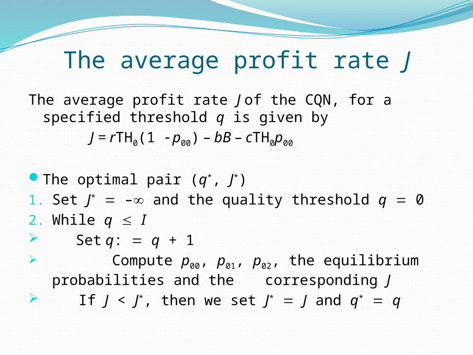
The average profit rate J of the CQN, for a specified threshold q is given by
J = rTH0(1 p00) – bB – cTH0p00
The optimal pair (q*, J*)1. Set J* – and the quality threshold q 02. While q I Set q: q + 1 Compute p00, p01, p02, the equilibrium
probabilities and the corresponding J If J < J*, then we set J* J and q* q

Numerical resultsIn all numerical experiments presented here the total number
of customers is M = 50We use eight distinct quality levels ( i = 0,…,7 )The production probabilities pi are based in the same
distribution as in the first example mentionedThe conditional probabilities are also the same with those in
the first exampleConcerning the optimal policy model, in the column “Policy
structure” at the results, we present the optimal policies for every quality level. For a certain quality level:
(0) : the optimal decisions are scrapping decision for all states (1) : the optimal decisions are selling decisions for all states (\) : there are both scrapping and selling decisions in the
state space

Examples and results for both optimal and threshold policy
Parameter values Optimal policy Threshold policy1 2 c r b Policy structure Average profit Average profit Quality threshold
__________________________________________________________________________________________ 1 0.1 55 4 4 0.35 111111\\ 51.255383 51.165181 level 5
1 0.1 55 4 4 0.45 111111\\ 51.221129 51.131003 level 5
1 0.1 55 4 4 0.6 111111\\ 51.169754 51.079778 level 5
1 0.1 55 4 4 0.8 111111\\ 51.101278 51.011384 level 5
1 0.1 55 4 4 1.1 111111\\ 50.998663 50.908852 level 5
1 0.1 55 4 4 1.35 111111\\ 50.913222 50.823410 level 5
_________________________________________________________________________________
1 0.1 55 4 3.5 0.35 1111111\44.649882 44.575442 level 6
1 0.1 55 4 4.5 0.35 111111\057.998738 57.896663 level 5
1 0.1 55 4 5 0.35 11111\\0 64.772343 64.642366 level 4
1 0.1 55 4 5.5 0.35 11111\\0 71.859395 71.718639 level 4
1 0.1 55 4 6 0.35 11111\00 78.949696 78.794912 level 4
_________________________________________________________________________________ 1
1 0.1 55 2.2 4 0.35 1111\\00 53.891926 53.424611 level 3
1 0.1 55 2.5 4 0.35 1111\\00 52.836943 52.733324 level 4
1 0.1 55 3 4 0.35 11111\\0 52.087461 51.985423 level 4
1 0.1 55 3.5 4 0.35 1111\\0070.723484 70.555552 level 3

Examples and results for both optimal and threshold policy
Parameter values Optimal policy Threshold policy 1 2 c r b Policy structure Average profit Average profit Quality
threshold_________________________________________________________________________________
0.8 0.1 55 4 4 0.35 1111111\ 48.989474 48.913564 level 6
0.9 0.1 55 4 4 0.35 111111\\ 50.202982 50.116805 level 5
1.1 0.1 55 4 4 0.35 111111\\ 52.150325 52.056024 level 5
1.4 0.1 55 4 4 0.35 111111\\ 54.177700 54.073082 level 5
_________________________________________________________________________________
1 0.08 55 4 4 0.35 111111\0 42.697024 42.617049 level 5
1 0.12 55 4 4 0.35 1111111\ 59.191805 59.099059 level 6
1 0.15 55 4 4 0.35 1111111\ 70.133711 70.033063 level 6
1 0.2 55 4 4 0.35 11111111 86.084805 85.982183 level 7
_________________________________________________________________________________
1 0.1 45 4 4 0.35 111111\\ 51.106237 51.016541 level 5
1 0.1 50 4 4 0.35 111111\\ 51.190849 51.100905 level 5
1 0.1 60 4 4 0.35 111111\\ 51.306170 51.215759 level 5
1 0.1 65 4 4 0.35 111111\\ 51.347163 51.256585 level 5
1 0.1 55 4 4 0.35 111111\0 51.576829 51.486063 level 5

ConclusionsThe mean profit rates of the two policies differ by less than
1% The optimal policy model can be a helpful tool for examining
the dynamics of quality in production and the way it affects customer satisfaction, market share and profitability
In cases where this approach is not easy to implement, a simple threshold-type control policy with reasonable computational requirements is proposed and appears to be a good approximation of the optimal policy
As a next step we intend to examine the case where customer satisfaction is affected by his previous state
Another extension is to consider the effect of waiting times in customer satisfaction