Diophantine Analysis

Jorn Steuding

Winter 2002/03Johann Wolfgang Goethe-Universitat Frankfurt

This course gives an introduction to the theory of Diophantine Approximations witha special emphasis on its impact to the field of Diophantine Equations. It reliesmainly on the nicely written books [9], [29] as well as the more general introduction[8] and the classics [21], [35]; historical details can be found in [11], [48] and onwww.history.mcs.st− andrews.ac.uk. Finally, we refer to [4] for modern perspectivesin this amazing and growing field.

We will use only standard notation. Special knowledge which is beyond the scopeof first courses in mathematics is (with some small exceptions) not necessary. Thereader can find some easy and some difficult exercises in the text which may help toget familar with the topic.

The author is very grateful to Iqbal Lahseb, Ernesto Girondo, Thomas Mullerand Matthias Volz for several remarks and corrections.

1 Introduction: three basic principles

Diophantus of Alexandria was a greek mathematician who lived around 250 A.D.,but virtually nothing more about his life is known than that what was written downon his tombstone:

God granted him to be a boy for the sixth part of his life,and adding a twelfth part to this, He clothed his cheeks with down.

He lit him the light of wedlock after a seventh part,and five years after his marriage He granted him a son.

Alas! late-born wretched child; after attainingthe measure of half his father’s life, chill Fate took him.

After consoling his grief by this science of numbersfor four years he ended his life. (cf. [52], p.55)

How old was Diophantus when he died? This riddle is an example for the kind ofproblems in which Diophantus was interested in. He wrote the influential monogra-phy Arithmetica which inspired Fermat (1607/08?-1665) to write down

1

It is impossible for a cube to be written as a sum of two cubesor a fourth power to be written as the sum of two fourth powers or,in general, for any number which is a power greater than the second

to be written as a sum of two like powers.I have a truly marvellous demonstration of this propositionwhich this margin is too narrow to contain. (cf. [52], p.66)

in his copy of Diophantus’ book, exactly there where the corresponding question forsquares is considered. In the modern language of algebra Fermat claimed to have aproof that all solutions of the equation

Xn + Y n = Zn (1)

in integers x, y, z are trivial, i.e. xyz = 0 , whenever n ≥ 3. Fermat never publisheda proof and, by the succcessless quest for a solution of Fermat’s last theorem overcenturies, mathematicians started to believe that Fermat actually had no proof.However, no counterexample was found. Only recently Wiles (supported by Taylorand the earlier works of many others) found a proof for Fermat’s last theorem (see[52] for the amazing story of this problem and its final solution). With our modernbackground in mathematics one may ask why the ancient Greek did not consider theFermat equation in its generality but only the quadratic case. Their point of viewwas inspired by at most three-dimensional geometry and only in the late works ofGreek mathematicians higher powers occur. They also had an advanced knowledgeon divisibility and prime numbers but no idea about the unique prime factorizationof the integers!

It is interesting that the exponent in the Fermat equation is crucial. As Dio-phantus explained in his book the equation (1) with exponent n = 2 has infinitelymany (non-trivial) solutions, for example

32 + 42 = 52, 52 + 122 = 132, 82 + 152 = 172, . . . .

These triples of integral solutions are called Pythagorean triples with regard toPythagoras’ theorem in geometry. However, the history of such triples dates at leastback to the ancient Babylonians four millenia ago. It is conjectured that they usedPythagorean triples for constructing right angles. Pythagoras (572-492 B.C.) foundnot only a proof that such triples yield right angles but gave also an infinitude ofprimitive (coprime) Pythagorean triples by the identity

(2n + 1)2 + (2n2 + 2n)2 = (2n2 + 2n + 1)2 for n ∈ N.

In the third century B.C. Euclid solved the problem of finding all solutions.

Exercise 1 Show that all positive integral solutions x, y, z of

X2 + Y 2 = Z2,

2

satisfying (x, y) = 1 and 2|x , are given by

x = 2ab, y = a2 − b2, z = a2 + b2,

where a and b are coprime integers of opposite parity and a > b . [Hint: each solution

satisfies x2 = z2 − y2 = (z + y)(z − y) .]

Note that this classification of the Pythagorean triples can be used to prove thatthe biquadratic case of (1) has only trivial solutions. Actually, Fermat combinedthis result with his method of infinite descent to prove that the slightly more generalequation

X4 + Y 4 = Z2

has no positive integral solutions (see [21], §13.3).We are living in a finite universe (there are only about 1080 atoms in our uni-

verse) which means that our world can be described using only rational numbers.However, for an understanding of the physical world as well as the abstract worldof mathematics this is not enough! The same equation which Euclid studied so suc-cessfully led some hundred years before to one of the great breakthroughs in ancientGreek mathematics. Hippasus, a pupil of Pythagoras, discovered that the set ofrational numbers is too small for the simple geometry of triangles and squares. Infact, he proved that the length of the diagonal of a unit square is irrational:

√2 =√

12 + 12 6∈ Q.

Nowadays this is taught at school, but for the Pythagoras school it was the deathof their philosophy that all natural phenomenon could be explained in integers. Itis said that Pythagoras sentenced Hippasus to death by drowning. This unkind actcould not stop the mathematical progress. In order to solve polynomial equationsand for the merits in analysis the mathematicians invented various new numbers:

N ⊂ Z ⊂ Q ⊂ R ⊂ C,

and even more as we will see in section 16; we refer the interested reader to thecollection [12] of excellently written surveys on numbers of all kinds. However, forthe first we shall only consider real numbers.

By Cantor’s diagonal argument we know that the set of real numbers R is un-countable whereas Q is countable. Therefore, almost all real numbers are irrational.We shall give a more advanced example than the square root of two. One of the fun-damental constants in analysis (and natural sciences) is the value of the exponentialfunction at one:

e =∞∑n=0

1

n!.

Theorem 1 e is irrational.

3

This result dates back to Euler in 1737, resp. Lambert in 1760; however theirapproach via continued fractions is rather difficult (we will return to this later).However, the following simple proof would have been possible in Euler’s times.

Proof. Suppose the contrary, then there exist positive integers a, b such that e = ab.

If m is an integer ≥ b then b divides m! and

α = m!

(e−

m∑n=0

1

n!

)= a

m!

b−

m∑n=0

m!

n!

is an integer. On the other side,

0 < α =∞∑

n=m+1

m!

n!<

1

m+ 1

∞∑k=0

(1

m+ 1

)k=

1

m,

which gives the contradiction. The theorem is proved. •

This proof reveals an important principle in the diophantine toolbox: the seriesconverges so fast that the limit cannot be of a restricted arithmetical nature!

The question whether a given real number is irrational seems to be simple on thefirst view. Actually, this is a rather difficult problem. For instance, it is unknownwhether the Euler-Mascheroni constant

γ = limN→∞

(N∑n=1

1

n− logN

)

is irrational. Another important constant is π , which we define as the smallestpositive root of the sine function.

Theorem 2 π is irrational.

The first proof of the irrationality of π was given by Lambert in 1761, also byusing continued fractions. The proof which we shall give now, as all other knownproofs, is slightly more difficult than the given one for e . This holds also in otherquestions around these two fundamental numbers. It seems that e has somehowmore structure than π . Our short but tricky proof is due to Niven [37].

Proof. We start with some preliminaries. For n ∈ N define

fn(x) =1

n!xn(1− x)n. (2)

Hence,

fn(x) =1

n!

2n∑j=n

cjxj with cj ∈ Z

and

0 < fn(x) <1

n!for 0 < x < 1. (3)

4

It is easy to find for the k -th derivative

(−1)kf (k)n (1) = f (k)

n (0) =

{0 if 0 ≤ k < n,k!n!ck if n ≤ k ≤ 2n;

(4)

here we used f (k)n (x) = (−1)kf (k)

n (1− x) and the Taylor expansion (or dumb com-putation). Note that all these values are integers.

We shall even show that π2 is irrational. Assume that π2 = ab

with positiveintegers a and b . We consider the polynomial

Fn(x) := bn(π2nfn(x)− π2n−2f (2)n (x)± . . .+ (−1)nf (2n)

n (x)).

Since bnπ2k = bn−kak ∈ Z for 0 ≤ k ≤ n , it follows in view of (4) that Fn(0), Fn(1) ∈Z . A short calculation shows

(F ′n(x) sin(πx)− πFn(x) cos(πx))′ = π2anfn(x) sin(πx).

With regard to sinπ = sin 0 = 0 this yields

In := πan∫ 1

0fn(x) sin(πx) dx = Fn(0) + Fn(1),

which is an integer. On the other side we get with regard to (3)

0 < In < πan

n!.

Since the factorial n! grows faster than an , the right hand side above can be made< 1 by choosing n sufficiently large. This gives the contradiction and the theoremis proved. •

Also this proof is very interesting: a problem concerning the arithmetic nature ofa given real number is solved by the construction of an appropriate sequence ofpolynomials with respect to its analytical behaviour!

As we have seen above almost all real numbers are irrational, but how to dealwith them in our finite world? Since Q is dense in R it is natural to search forrational approximations (but Q has also the disadvantage of beeing very thin inR). For example, we can think about some machine which has to compute anapproximation to the circumference of a circle with given radius. For that we haveto construct some mechanism with gears which approximates the ratio π : 1, butthis needs a good approximation of the irrational

π = 3.14159 26535 . . .

by rational numbers. It is interesting to see how this problem was solved in formertimes:

• The Rhind Papyrus (≈ 1650 B.C.): π ≈ 4(

89

)2= 3.16045 . . . ;

5

• Old testament (≈ 1000 B.C.): π ≈ 3;

• Archimedes (287-212 B.C.): π ≈ 227

= 3.14285 . . . ;

• Tsu Chung Chi (≈ 500 A.D.): π ≈ 355113

= 3.14159 29920 . . . .

We shall not speak about the attempt of an american politician to attach π by lawthe value 3.2 in 1897; for this and more on π see [5]. More useful is the rhyme

Now I want a drink, alcoholic of course,after the heavy lectures involving quantum mechanics!

Recently, Kanada and Takahashi computed π up to more than 206 billion digits.This precision is beyond any use in applications (the Planck constant 10−33 is thesmallest unit in quantum mechanics) but interesting from a mathematical pointof view. Since Q is dense in R , for any real number there exist infintely manyrational approximations. Moreover, we can approximate with any assigned degreeof accuracy. But what are good and what are bad approximation among them or,what is the same, how rapidly can we approximate? A natural measure is thedenominator. Let α be any real number, then we say that p

q∈ Q with q ≥ 1 is a

best approximation to α if

|qα− p| < |Qα− P | for all Q < q,

where P,Q ∈ Z ; necessarily a best approximation is a reduced fraction. In particu-lar, a best approximation p

qto α is the nearest rational number with denominator

≤ q , but not vice versa! For example, the first best approximations to π are

3

1,

22

7,

333

106,

355

113,

1 03993

33102, . . .→ π.

It is remarkable that the fractions given by Archimedes and of Tsu Chung Chi arebest approximations. How could they do that in these dark ages without computers?In general, finding good rational approximations to a given irrational number is adifficult task.

In honour of Diophantus we speak about

• Diophantine Approximations when we search for rational approximationsto rational or irrational numbers;

• Diophantine Equations when we investigate polynomial equations on solu-tions in integers (or rationals).

As we shall see both areas are linked in various directions. For instance, we ask forsolutions of the equation

38X − 15Y = 1 (5)

6

in integers. One approach to answer this question offers Euclid’s algorithm. Bydivision with remainder for any positive integers a, b with b > a there existinteger q, r such that

b = aq + r with 0 ≤ r < a.

Now define r−1 := b, r0 := a . Then, successive application of division with remainderyields the Euclidean algorithm:

For j = 0, 1, . . . do rj−1 = qj+1rj + rj+1 with 0 ≤ rj+1 < rj . (6)

Since the sequence of remainders is strictly decreasing, the algorithm finishes afterfinitely many, say n steps and, by simplest divisibility properties, it turns out thatthe last non-vanishing remainder rn is equal to the greatest common divisor of aand b .

Exercise 2 Show that the running time (i.e. the number of steps) in the Euclideanalgorithm is

n ≤2

log 2log(b+ 1).

Can you describe the smallest numbers a, b for which the algorithm needs exactly nsteps? Can you improve the previous estimate?

From an algorithmical point of view it is of advantage to use a modified Euclid-ean algorithm which works with the nearest integer and not with the next largerinteger. However, for our purpose the above stated version is sufficient. Readingthe Euclidean algorithm backwards, we get a concrete integral solution of the linearequation

bX − aY = (a, b), (7)

say x0, y0 . It is easily seen that then all integral solutions to the latter diophantineequation are given by(

x

y

)=

(x0

y0

)+

1

(a, b)

(a

b

)· Z. (8)

From here it is only a small step to

Theorem 3 The linear diophantine equation bX − aY = c with integers a, b, c issolvable if and only if (a, b)|c .

We return to our example. It may be a little bit surprising to see that thesolutions of (5) yield good approximations to 15

38and vive versa:

. . . , 38 · (−13)−15 · (−33) = 1 , 38 · 2− 15 · 5 = 1 , 38 · 17− 15 · 43 = 1, . . .

7

vs.x

y=

2

5,

13

33,

17

43. . .→

15

38;

note that the solutions x, y with |y| < 38 give even the best approximations xy

to 1538

. However, this is not too surprising. We may rewrite each solution of ourmodified equation as

x

y=

15

38+

1

38y,

and since the second term is rather small, we see a certain relation between approx-imations to 15

38and our integral solutions.

Exercise 3 Prove that the best approximations xy

to any given ab∈ Q exactly cor-

respond to those solutions x, y ∈ Z of (7) with |y| < b .

With regard to our previous observations we can solve the linear diophantine equa-tion (7) by searching for the best approximations to a

b. This was first discovered by

Aryabhata around 550 A.D. However, this example is only the top of an iceberg:certain diophantine equations can be investigated by studying a related problem inthe theory of diophantine approximations!

2 Dirichlet’s approximation theorem

It is much more interesting to approximate irrational numbers than rationals. In1842 Dirichlet proved the first but fundamental approximation theorem.

Theorem 4 If α is irrational, then there exist infinitely many rational numbers pq

such that ∣∣∣∣∣α− p

q

∣∣∣∣∣ < 1

q2; (9)

this property characterizes irrational numbers, i.e., a rational α allows only finitelymany approximations p

qwith (9).

In particular, there exist infinitely many best approximations to any given irrationalnumber (in contrast to rationals; see Exercise 3).

The following original proof relies on the pigeonhole principle which statesthat if n + 1 objects are distributed to n boxes, then at least one box contains atleast two objects (which is easily seen by a contradiction argument or induction).

Proof. We define the integral part and the fractional part of a real number xby

[x] = max{z ∈ Z : z ≤ x} and {x} = x− [x],

respectively. Let Q be a positive integer. The numbers

0, {α}, {2α}, . . . , {Qα}

8

define Q+ 1 points distributed among the Q disjoint intervals

j − 1

Q≤ x <

j

Qfor j = 1, . . . Q.

By the pigeonhole principle there has to be at least one interval which contains atleast two numbers {kα} > {`α} , say, with 0 ≤ k, ` ≤ Q . It follows that

0 ≤ {kα} − {`α} = kα− [kα]− `α + [`α]

= {(k − `)α} + [(k− `)α] + [`α]− [kα]︸ ︷︷ ︸∈Z

<1

Q.

Obviously, the integral parts add up to zero. Hence, setting q = k − ` we obtain

{qα} = {kα} − {`α} <1

Q.

With p := [qα] it follows that∣∣∣∣∣α− p

q

∣∣∣∣∣ =|qα− p|

q<{α}

qQ<

1

qQ, (10)

which implies the estimate (9) (since q < Q).Now assume that α is rational, say α = a

b. If α 6= p

q, then∣∣∣∣∣α− p

q

∣∣∣∣∣ =|aq − bp|

bq≥

1

bq(11)

and (9) involves q < b , which proves that there are only finitely many pq

with (9).Now suppose that α is irrational and that there exist only finitely many solutions

p1

q1, . . . , pn

qnto (9). Since α 6∈ Q , we can find a Q such that∣∣∣∣∣α − pj

qj

∣∣∣∣∣ > 1

Qfor j = 1, . . . , n,

contradicting (10). The theorem is proved. •

Notice that by this proof it is impossible to compute approximations without bigcomputational effort.

Dirichlet’s approximation theorem can be extended to a first irrationality cri-terium:

Exercise 4 Prove that if there are infinitely many coprime solutions p, q of

|qα− p| < q−δ

with a fixed δ > 0, then α is irrational. [Hint: using (11) show that for rational α the sets

of possible denominators q and of possible numerators p are finite.]

Deduce the irrationality of∞∑n=1

2−n!.

[The idea behind should be compared with our proof of the irrationality of e .]

9

More irrationality criteria of this type can be found in [8], §5.Dirichlet’s proof yields also an extension to simultaneous approximation prob-

lems.

Exercise 5 Prove that if α1, . . . , αn are arbitray real numbers, then the system ofinequalities ∣∣∣∣∣αj − pj

q

∣∣∣∣∣ < q−1− 1n for j = 1, . . . , n

has at least one solution p1, . . . pn, q ∈ Z ; if at least one αj is irrational, then it hasan infinitude of solutions.

We say that α is approximable by rationals of order κ if there exists apositive constant c(α) , depending only on α , such that∣∣∣∣∣α − p

q

∣∣∣∣∣ < c(α)

qκ

has an infinity of solutions pq

. In a sense, κ indicates the speed of convergence ofthe sequence p

qto α . With view to our previous observations we see that

• any rational α is approximable of order 1, and to no higher order (by Exercises3 and 5);

• any irrational α is at least approximable of order 2 (by Theorem 4).

It is a natural question to ask for improvements of Dirichlet’s theorem. Khintchineproved in the 1930s a remarkable result which states that the set of numbers whichmay allow a stronger approximation has measure null, i.e given any positive ε ,the set can be covered by a countable number of intervals of total length < ε .

Theorem 5 Suppose that ψ is a positive function such that

∞∑q=1

ψ(q)

converges. Then for almost all α (i.e. with exceptions which have measure 0), thereis only a finite number of solutions p, q ∈ Z to the inequality

|qα− p| < ψ(q). (12)

The proof relies on Dirichlet’s idea of locating the real number α in question insmall intervals.

Proof. Given ε > 0, we can find an integer Q such that∑q≥Q

ψ(q) <ε

2.

10

Now consider those α for which the inequality (12) has infinitely many solutions.

Now for each q ≥ Q consider the intervals of radius ψ(q)q

surrounding the rational

numbers 0q, 1q, . . . , q−1

q. Consequently, each α will lie in one of these intervals. The

measure of these intervals is ∑q≥Q

q ·2ψ(q)

q< ε,

which proves the theorem. •

For example, we may take ψ(q) = q−1(log q)−1−ε . Thus almost all numbers cannotbe approximated by an order 2+ε . A more subtile characterization of real numberswith respect to the order of approximation seems to be a rather difficult task. Wewill return to this problem in a later section.

We shall briefly give an interesting application of Dirichlet’s approximation the-orem to dense sequences. As we have seen above for any given real α we can findintegers q for which qα differs from an integer by as little as we please. Kronecker’scelebrated approximation theorem from 1891 considers the inhomogeneous case.

Theorem 6 If α is irrational, η ∈ R is arbitrary, then for any N ∈ N there existQ ∈ N with Q > N and P ∈ Z such that

|Qα− P − η| <3

Q.

Proof. By Theorem 4 there are integers q > 2N and p such that

|qα− p| <1

q.

Suppose that m is the integer, or one of the two integers, for which

|mη − q| ≤1

2.

In view of Theorem 3 and in addition (7) we can write m = px− qy , where x andy are integers and |x| ≤ 1

2q . Since

q(xα− y − η) = x(qα− p)− (qη −m),

we find

|q(xα− y − η)| <1

2q ·

1

q+

1

2= 1.

Setting Q = q + x and P = p+ y yields

N <1

2q ≤ Q ≤

3

2q,

and thus

|Qα− P − η| ≤ |xα− y − η|+ |qα− p| <2

q≤

3

N.

11

This proves the theorem. •

In particular, Kronecker’s approximation theorem has interesting consequences ondense sequences:

Exercise 6 Show that the sequence ({nα}) lies dense in [0, 1] if and only if α isirrational.

Much more can be said about such sequences. In fact, one can show that if andonly if α is irrational, the sequence (nα) is uniformly distributed modulo 1,i.e., the correct proportion of points {nα} lies in an arbitrary subinterval (a, b) of(0, 1). On the other side, it is not difficult to show that for example the fractionalparts of logn prefer small values where, as usual in number theory, log n is thelogarithm to base e . But it is yet unproved that the sequence exp(n) is uniformlydistributed modulo 1. For a rigorous definition of uniform distribution, the currentknowledge in this field and its various applications we refer the reader to [23].

Another interesting application of Kronecker’s approximation theorem is theproblem of the reflected light ray in plane geometry due to Konig and Szucs. Thesides of a square are reflecting mirrors. A ray of light leaves a point inside the squareand is reflected in the mirrors. One can show that its path is closed and periodicif and only if the angle between a side of the square and the initial direction of theray has a rational tangent; otherwise the ray of light passes arbitrarily near to everypoint of the square. For the proof of this entertaining billiards see [21], §23.3.

In the following sections we will meet two different approaches for more detailedstudies concerning diophantine approximations.

3 The Farey sequence

Farey fractions were introduced by Haros in 1802 and (independently) by Farey in1816. However, Cauchy was the first who studied them systematically.

For any positive integer n the Farey sequence Fn of order n is the orderedlist of all reduced fractions in the unit interval having denominators ≤ n :

Fn ={a

b∈ Q : 0 ≤ a ≤ b ≤ n with (a, b) = 1

}.

For example,

F1 ={

0

1,1

1

}⊂ F2 =

{0

1,1

2,1

1

}⊂ F3 =

{0

1,1

3,1

2,2

3,1

1

}⊂ . . . . (13)

Clearly, Fn ⊂ Fn+1 . Further, each rational in the unit interval occurs sooner orlater in the Farey sequence. Hence, the Farey sequence is building Q modulo Z .In particular, this construction proves that Q is countable. We can be a bit moreprecise to get a feeling for the size of Fn . It is easily seen that the number of Fareyfractions in Fn is related to Euler’s totient ϕ(b) which counts the number of positive

12

coprime integers a ≤ b . With some knowledge on arithmetical functions one canshow the asymptotic formula

]Fn = 1 +∑b≤n

ϕ(b) =3

π2n2 +O(n log n),

where f(x) = O(g(x)) with a positive function g(x) denotes that

lim supx→∞

|f(x)|

g(x)is bounded.

Two consecutive elements in Fn are called neighbours. One fundamental prop-erty of Farey fractions is the spacing of neighbours in the unit interval.

Theorem 7 For any neighbours ab< c

din Fn ,

bc− ad = 1.

In particular, under the assumptions of the theorem

c

d−a

b=bc− ad

bd=

1

bd.

This shows that Fn is not uniformly, but in a diophantine sense, optimally distrib-uted, namely with regard to the denominators.

Proof. Consider the diophantine equation

bX − aY = 1.

Since a and b are coprime, by Theorem 3 and in addition (8) there exists a solutionx, y ∈ Z with n−b < y ≤ n . Consequently, also x and y are coprime, and thereforexy∈ Fn . It is easy to compute that

x

y=a

b+

1

by>a

b. (14)

Now suppose that cd< x

y, then

x

y−c

d=dx− cy

dy≥

1

dy.

Further,c

d−a

b=bc− ad

bd≥

1

bd.

These estimates imply

x

y−a

b=x

y−c

d+c

d︸ ︷︷ ︸=0

−a

b≥

1

bd+

1

dy=y + b

bdy>

n

bdy.

13

In view of (14) it follows that n < d , contradicting cd∈ Fn . Thus we have c

d= x

y

which proves the theorem. •

Note that the proof gives a rule for the computation of the successor of a Fareyfraction a

bin Fn . This term is also related to the former right neighbour of a

b. We

define the mediant of ab, cd∈ Fn by a+c

b+d(like adding two fractions the wrong way).

If ab< c

d, then it is easily seen that

a

b<a+ c

b + d<c

d.

The mediant is a mean value, but different to other more common mean valueslike the arithmetic or the geometric mean value, the mediant is not monotonic: forexample,

1

6<

1

3and

23

36<

2

3, but

1 + 23

6 + 36=

4

7>

1

2=

1 + 2

3 + 3.

This phenomenon is well-known in statistics where it is called Simpson’s paradox(though it is not paradox).

Exercise 7 Show that for any given pair AB< C

Dthere exist infinitely many pairs

ab< A

B, cd< C

Dsuch that

a+ c

b+ d>A+B

C +D.

For this and more see [53].The importance of the notion of mediants becomes clear by investigating (13).

The process of taking mediants builds the Farey sequence out of 01

and 11.

Theorem 8 The fractions which belong to Fn but not to Fn−1 are mediants ofelements of Fn .

In particular, the property for two consecutive Farey fractions ab, cd

of being neigh-bours gets lost in Fn if n ≥ b+ c .

Proof. With regard to Theorem 7 we have for consecutive Farey fractions

a

b<x

y<c

d

in Fn the identities

bx− ay = 1 and cy − dx = 1.

Multiplying this with c and a , resp. d and b , yields

x(bc− ad) = a+ c and y(bc− ad) = b+ d,

14

which implies the second assertion. •

The Farey sequence is related to an amazing geometry, discovered by Ford in the1940s. We may embed the unit interval [0, 1] into the complex plane C and definefor each a

b∈ Fn the so-called Ford circle

C(a

b

)={z ∈ C :

∣∣∣∣z − (ab +i

2b2

)∣∣∣∣ =1

2b2

},

where as usual i :=√−1. Ford circles provide an interesting sphere packing:

Exercise 8 Prove that two distinct Ford circles i) have an empty intersection of theinteriors, and ii) are tangent if and only if they are associated to neighbours in theFarey sequence.

We return to our problem to find explicitly good approximations to a given α in theunit interval. If we want to get a rational approximation with denominator ≤ n ,then we only have to look for the Farey fraction a

b∈ Fn with minimal distance to

α . Further approximations can be found by taking the mediants. It is obvious howone can use Ford circles to localize visually these Farey fractions.

Exercise 9 The golden ratio is given by g = 12(√

5−1) . Find all best approxima-tions p

qto g with a denominator q ≤ 100 . Do you see some hidden law? [Compare

your observations with the numbers for which the Euclidean algorithm is extremal; see Exercise 2.]

Compute the quantities q|qg− p| . Do the same for α =√

2 .

The Farey dissection of the continuum is a very usefool tool in the theory of diophan-tine approximations. It provides not only an approach to explicit approximationsbut also an improvement of Dirichlet’s approximation theorem, found by Hurwitzin 1891.

Theorem 9 If α is irrational, then there exist infinitely many rational numbers pq

such that ∣∣∣∣∣α− p

q

∣∣∣∣∣ < 1√

5q2;

the constant√

5 is best possible.

Proof. Suppose that ab< c

dare those neighbours in Fn for which

a

b< α <

c

d.

Without loss of generality we assume that α > a+cb+d

(since we may replace α by1− α otherwise). If now

α−a

b≥

1√

5b2, α−

a+ c

b+ d≥

1√

5(b+ d)2and

c

d− α ≥

1√

5d2, (15)

15

then we obtain by adding these inequalities

c

d−a

b≥

1√

5

(1

b2+

1

d2

)=

1√

5

b2 + d2

b2d2

andc

d−a+ c

b+ d≥

1√

5

(1

(b+ d)2+

1

d2

)=

1√

5

(b+ d)2 + d2

(b+ d)2d2.

On the other side, Theorem 7 and 8 give upper bounds for these quantities, whichlead to the inequalities

√5bd ≥ b2 + d2 and

√5(b+ d)d ≥ (b+ d)2 + d2.

Adding both inequalities gives

√5(d2 + 2bd) ≥ 3d2 + 2bd+ 2b2,

resp.0 ≥ 4b2 − 4(

√5− 1)bd+ (5− 2

√5 + 1)d2 = (2b− (

√5− 1)d)2,

which is impossible since b, d ∈ Z but√

5 6∈ Q . Thus, with view to (15) at leastone of the inequalities∣∣∣∣α − a

b

∣∣∣∣ < 1√

5b2,

∣∣∣∣α − a+ c

b+ d

∣∣∣∣ < 1√

5(b+ d)2and

∣∣∣∣α− c

d

∣∣∣∣ < 1√

5d2

holds. Since α is irrational this argument yields the existence of infinitely manysuch rational approximations by sending n→∞ . The first assertion of the theoremis proved.

For the second one recall the definition of the golden ratio g = 12(√

5− 1). We

consider the polynomial P (X) := X2 + X − 1. With G := 12(√

5 + 1) we haveP (X) = (X − g)(X +G) . Now assume that∣∣∣∣∣g − p

q

∣∣∣∣∣ < 1

Cq2

with p ∈ Z, q ∈ N . Then

∣∣∣∣∣P(p

q

)∣∣∣∣∣ =

∣∣∣∣∣g − p

q

∣∣∣∣∣ ·∣∣∣∣∣G+

p

q

∣∣∣∣∣ =

∣∣∣∣∣g − p

q

∣∣∣∣∣ ·∣∣∣∣∣∣∣G+g − g︸ ︷︷ ︸

=0

−p

q

∣∣∣∣∣∣∣ <√

5

Cq2+

1

C2q4.

On the other side, ∣∣∣∣∣P(p

q

)∣∣∣∣∣ =|p2 + pq − q2|

q2≥

1

q2,

which implies C ≤√

5. This proves the second assertion. •

16

By the proof it seems that the restriction on C depends mainly on the fact that weinvestigated approximations to g . We call a real number α quadratic irrationalif it is the root of an irreducible quadratic polynomial with integral coefficients, theminimal polynomial of α . Obviously, any such α is of the form

α =a+ b

√d

cwith a, b ∈ Z, c, d ∈ N, (16)

where d is squarefree, i.e., all prime divisors of d have multiplicity one; in partic-ular, a quadratic irrational is irrational.

Exercise 10 Suppose that α is the real quadratic irrational with minimal polyno-mial aX2 + bX + c . Show that for C >

√b2 − 4ac the inequality∣∣∣∣∣α− p

q

∣∣∣∣∣ < 1

Cq2

has only finitely many solutions p, q ∈ Z . Compare this with Exercise 9. Try to formulatea conjecture for quadratic irrationals.

Another interesting topic in context of the Farey sequence is the Riemannhypothesis which claims that the prime numbers are as uniformly distributed aspossible, namely

π(x) =∫ x

2

du

log u+O

(x

12

+ε)

for any ε > 0, (17)

where π(x) counts the number of primes ≤ x . This is problem number 8 of Hilbert’sfamous list of 23 problems which he presented at the International Congress ofMathematicians in Paris in 1900. The Riemann hypothesis is yet unsolved (actuallyit is one of the seven Millenium problems). Surprisingly, is related to the deviationof the Farey sequence from being uniformly distributed. Denote the j -th element ofFn by fj (ordered by their size). Then, by a result of Franel, Riemann’s hypothesisis true if and only if

]Fn∑j=1

∣∣∣∣∣fj − j − 1

]Fn

∣∣∣∣∣ = O(n

12

+ε)

(see [24] for the details).Further applications of Farey fractions are error-free computing strategies (details

can be found in [46], §5.12) and the dissection of the complex unit circle with regardto the circle method (see [24]).

4 Continued fractions

The powerful tool of continued fractions was first systematically studied by thedutch astronomer Huygens in the 17-th century, motivated by technical problems

17

while constructing a model of our solar system. The most detailed textbook on thistopic is the classic [38].

Recall the intimate relation between the approximations to a given rational ab

and the solutions of linear diophantine equations (7), obtained by the Euclideanalgorithm. We may rewrite the Euclidean algorithm (6) by

rj−1

rj=

[rj−1

rj

]+rj+1

rjwith 0 ≤ rj+1 < rj. for j = 0, 1, . . . , n (18)

until rn 6= 0. Setting aj =[rj−1

rj

], we obtain

r−1

r0= a0 +

(r0

r1

)−1

= a0 +1

a1 +(r1r2

)−1 = . . . .

The first of these identities yields the integral part as an approximation to therational r1

r0. Using more and more of these identities, we obtain better and better

approximations, and among them we can even find all best approximations. Weshall give an example: a solar year has

365 days 5 hours 48 minutes and 45, 8 seconds ≈ 365 +419

1730days.

Unfortunately, this is not an integer, so how to create a good calendar? With viewto (18) we find

1730

419= 4 +

54

419,

resp.

365 +419

1730= 365 +

(1730

419

)−1

≈ 365 +1

4,

which is nothing else than Caesar’s calendar, i.e., a leap year each fourth year. Bythe full Euclidean algorithm we get

365 +419

1730= 365 +

1

4 +1

7 +1

1 +1

3 +1

6 +1

2

.

Using this without the last fraction 12

gives

365 +419

1730≈ 365 +

194

801;

this our present calendar (six leap years are deleted in 800 years), the Gregoriancalender, introduced by pope Gregor XIII in 1582.

18

Exercise 11 The lunar month has 29.53 days; approximate the solar year by365.24 . Recover the Metonic cycle of seven leap month every 19 years from a goodapproximation to 365.24

29.53by use of the Euclidean algorithm. This is used in the jewish

calendar.

We call

a0 +1

a1 +1

a2 +...

+1

an−1 +1

aN

,

where a0 ∈ Z and an ∈ N for 1 ≤ n < N and aN ≥ 1, a finite simple continuedfraction. Here means simple that all numerators are equal to one; it is possible toallow other values but in what follows we will, more or less, deal only with simplecontinued fractions; therefore we may omit the word simple in the sequel. The anare called partial denominators. For brevity we denote the continued fractionabove [a0, a1, a2, . . . , aN ] .

First, we shall consider [a0, . . . , aN ] as a function in the variables a0, . . . aN . Wefind by induction on n

[a0, a1, . . . , an] =[a0, a1, . . . , an−1 +

1

an

](19)

= a0 +1

[a1, . . . , an]= [a0, [a1, . . . , an]].

For n ≤ N we call [a0, a1, . . . , an] the n-th convergent to [a0, a1, . . . , aN ] anddefine

p−1 = 1 , p0 = a0 and pn = anpn−1 + pn−2, (20)

q−1 = 0 , q0 = 1 and qn = anqn−1 + qn−2.

The computation of the convergents is easily ruled by means of

Theorem 10 The functions pn, qn satisfy

(i) pnqn

= [a0, a1, . . . , an] ,

(ii) pnqn−1 − pn−1qn = (−1)n ,

(iii) pnqn−2 − pn−2qn = (−1)nan .

Proof We prove the first assertion by induction on n . The cases n = 0 is obvious.The case n = 1 is easily computed by

[a0, a1] =a1a0 + 1

a1=p1

q1.

19

Now assume that the formula in question holds for n . Then, in view of (19) andthe recursion formulae for the pn, qn

[a0, a1, . . . , an, an+1] =

[a0, a1, . . . , an +

1

an+1

]

=

(an + 1

an+1

)pn−1 + pn−2(

an + 1an+1

)qn−1 + qn−2

=an+1pn + pn−1

an+1qn + qn−1=pn+1

qn+1,

which proves (i). In view of this we have

pnqn−1 − pn−1qn = (anpn−1 + pn−2)qn−1 − pn−1(anqn−1 + qn−2)

= −(pn−1qn−2 − pn−2qn−1).

Repeating this argument with n− 1, n− 2, . . . , 2 proves (ii). Consequently, pn andqn are coprime. Further,

pnqn−2 − pn−2qn = (anpn−1 + pn−2)qn−2 − pn−2(anqn−1 + qn−2)

= an(pn−1qn−2 − pn−2qn−1),

and the last assertion follows from the second one. •

The continuous fraction expansion is not unique since

[a0, a1, a2, . . . , aN ] = [a0, a1, a2, . . . , aN − 1, 1],

but nearly unique. With regard to our previous observations it is easily seenthat any rational number has a representation as a finite continued fraction[a0, a1, a2, . . . , aN ] , which is unique if 1 < aN ∈ N . By Theorem 10 we get abetter understanding between the solutions of linear diophantine equations (7) andbest approximations:

Exercise 12 Calculate the continued fraction for 1538

and compare its convergentswith the approximations found in Section 1. Give a further proof of Exercise 3 byuse of Theorem 10.

We can rewrite the algorithm for computing the continued fraction of a rationalα =: α0 by the iteration

αn = [αn] +1

αn+1

for n = 0, 1, . . . ,

and setting an = [αn] . Obviously, if α is rational the iteration stops after finitelymany steps. Otherwise, if α is irrational, then the iteration does not stop and weget by this procedure

α = [a0, a1, a2, . . .].

20

[a0, a1, a2, . . .] is an infinite continued fraction but the first thing we have to askis whether the underlying infinite process is convergent? Theorem 10 remains validand with regard to its second assertion

α−pn

qn=αn+1pn + pn−1

αn+1qn + qn−1

−pn

qn=

(−1)n

qn(αn+1qn + qn−1). (21)

Since the qn are strictly increasing for n ≥ 2, the sequence of convergents is alter-nating

p0

q0<p2

q2< . . . < α < . . . <

p3

q3<p1

q1.

Thus, we have

Theorem 11 If α is irrational, then∣∣∣∣∣α − pn

qn

∣∣∣∣∣ < 1

qnqn+1;

in particular,

α = limn→∞

pn

qn= [a0, a1, a2, . . .].

It is easily shown that the continued fraction expansion of any irrational number isuniquely determined. Hence, conversely, we can introduce the set of real numbersR via continued fractions!

With view to Theorem 11 it becomes visible what an important role continuedfractions play in the theory of diophantine approximations. Firstly, it gives a thirdproof of Dirichlet’s approximation theorem. In view of (21) we have even

Exercise 13 Prove that among two consecutive convergents to any irrational αthere is at least one satisfying ∣∣∣∣∣α− p

q

∣∣∣∣∣ < 1

2q2.

Furthermore, if pq

is a solution of the latter inequality, then pq

is a convergent to α .

One can go further. Actually, among three consecutive convergents to any irrationalα there is at least one satisfying the inequality in Hurwitz’ theorem. Thus, weobtain explicitly as many good approximations to a given irrational as we please.For instance, a short computation gives the sequence of convergents to π

[3] = 3, [3, 7] =22

7, [3, 7, 15] =

333

106,

[3, 7, 15, 1] =355

113, [3, 7, 15, 1, 292] =

1 03993

33102, . . . ,

which are located as follows

3 <333

106<

1 03993

33102< . . . < π < . . . <

355

113<

22

7;

we observe that the sequence of convergents covers the best approximations! Thisis not a miracle as Lagrange proved in 1770:

21

Theorem 12 Let α be any irrational number with convergents pnqn

. If n ≥ 2 andp, q are positive integers satisfying 0 < q ≤ qn and p

q6= pn

qn, then

|qnα − pn| < |qα− p|.

This so-called law of best approximations shows that we cannot do better thanapproximating an irrational number by its convergents!

Proof. We may suppose that p and q are coprime. Since

|qnα− pn| < |qn−1α − pn−1|,

it is sufficient to prove the assertion under the assumption that qn−1 < q ≤ q ; thefull statement of the theorem follows then by induction on n . If q = qn , then p 6= pnand it follows that ∣∣∣∣∣pq − pn

qn

∣∣∣∣∣ ≥ 1

qn.

But ∣∣∣∣∣α− pnqn

∣∣∣∣∣ ≤ 1

qnqn+1<

1

2qn

by Theorem 11. Thus ∣∣∣∣∣α − pnqn

∣∣∣∣∣ <∣∣∣∣∣α− p

q

∣∣∣∣∣ ,which implies the inequality in question after multiplication with q = qn . Nowsuppose that qn−1 < q < qn . The system of linear equations

pnX + pn−1Y = p and qnX + qn−1Y = q

has the unique solution

x =pqn−1 − qpn−1

pnqn−1 − pn−1qn= ±(pqn−1 − qpn−1) , y =

pqn − qpnpnqn−1 − pn−1qn

= ±(pqn − qpn).

Hence, x and y are integers, neither is zero. Obviously, x and y have oppositesign. Since qnα− pn and qn−1α− pn−1 have opposite sign as well, x(qnα− pn) andy(qn−1α − pn−1) have the same sign. Since

qα− p = x(qnα − pn) + y(qn−1α − pn−1),

we obtain|qα− p| > |qn−1α− pn−1| > |qnα − pn|,

which was to show. •

22

5 The irrationality of ζ(3)

The Riemann zeta-function is defined by

ζ(s) =∞∑n=1

1

ns=∏p

(1−

1

ps

)−1

for s > 1, where the so-called Euler product is taken over all prime numbers.The identity between the series and the product may be regarded as an analyticversion of the unique prime factorization in Z . This analytic approach was foundby Euler in 1737 and gives a first glance on the intimate relation between ζ(s)and the distribution of prime numbers. For instance, assume that there are onlyfinitely many primes, then the product converges throughout the complex plane, incontradiction to the divergence of the harmonic series (i.e, the singularity of ζ(s) ats = 1). Thus, there are infinitely many prime numbers. However, for more deeperstudies one has to consider ζ(s) as a function of a complex variable. (see [24] formore details on this amazing link between analysis and number theory).

The values of the zeta-function taken at the integers are of special interest innumber theory. Euler showed that

ζ(2n) = (−1)n−1 (2π)2n

2(2n)!B2n for n ∈ N,

where Bk is the k -th Bernoulli number defined by

z

exp(z)− 1=∞∑k=0

zk

k!Bk;

note that Bk is rational. However, nearly nothing is known about the values takenat the odd integers (this is related to the trivial zeros of ζ(s) at s = −2n, n ∈ N).It was a senstaion when Apery proved in 1978

Theorem 13 ζ(3) is irrational.

We can only give a sketch of the proof; for the exciting story behind and more detailson the proof see [39]. The first step is the recursion formula

n3un + (n− 1)3un−2 = (34n3 − 51n2 + 27n − 5)un−1 for n ≥ 2.

We define sequences an and bn generated by this recursion and the initial values

a0 = 0 , a1 = 6 and b0 = 1 , b1 = 5.

It turns out that bn ∈ Z and an ∈ Q with denominators dividing 2[1, 2, . . . , n]3 ,where [1, 2, . . . , n] denotes here the least common multiple of 1, 2, . . . , n . Multiply-ing this recursion formula with u = a by bn−1 and additionally the same with u = bby an−1 , we get

n3(anbn−1 − an−1bn) = (n− 1)3(an−1bn−2 − an−2bn−1).

23

Since a1b0 − a0b1 = 6 we obtain

anbn−1 − an−1bn =6

n3. (22)

This leads to an example of a non-simple continued fraction

ζ(3) =6

5−16

117−...

−

n6

34n3 + 51n2 + 27n + 5− . . .

;

this differs from the expansions which we investigated before but it is convergenttoo. One can deduce from (22)∣∣∣∣ζ(3) −

an

bn

∣∣∣∣ =∞∑

m=n+1

6

m3bmbm−1= O

(1

b2n

).

It is easy to compute by the recursion formula that

bn � αn , where α = (1 +√

2)4.

By the prime number theorem, which is a weaker form of (17), it can be shown that

[1, 2, . . . , n] =∏p≤n

p[lognlogp ] ≤

∏p≤n

n = nπ(n) � en.

Now setting pn = 2an[1, 2, . . . , n]3 and qn = 2bn[1, 2, . . . , n]3 (which are both inte-gers by our remark above), we obtain qn � αne3n and

|qnζ(3) − pn| = O(q−δn

)with δ =

logα − 3

logα + 3= 0.08052 . . . .

This proves the theorem in view of Exercise 5.

Apery’s discovery started intensive research on this topic with the aim to obtainsimilar results for other values of ζ(s) . Beukers found a different proof for ζ(3) 6∈ Qby using Legendre polynomials, i.e., for n ∈ N the n-th derivative of the polynomialdefined in (2). However, it is still open whether ζ(5) or any other value taken atpositive odd integers is irrational. Recently, Rioval proved that there are infinitelymany irrational numbers in the set of odd zeta-values and Zudilin showed that atleast one of the four numbers ζ(5), ζ(7), ζ(9) and ζ(11) is irrational (cf. [61]).

6 Quadratic irrationals

Leonrado da Pisa (1170-1250) wrote the influential book Liber abaci in which heinvented the arabic ciphers and zero to Europe. Furthermore, he introduced theFibonacci numbers

1, 1, 2, 3, 5, 8, 13, 21, 34, 55, 89, . . . ,

24

defined by the recursion

F0 := F1 := 1 and Fn+1 = Fn + Fn−1 for n ∈ N.

In view of (20) it follows immediately that

limn→∞

FnFn−1

= [1, 1, 1, , . . .], (23)

but what is the value of this limit? If we denote this limit by x , then x = 1 + 1x

,which shows that x has to be a root of the quadratic polynomial X2−X−1 = (X−G)(X + g) which we already know from the proof of Hurwitz’ theorem. Thus, G =[1, 1, 1, . . .] and g = 1

G= [0, 1, 1, 1, . . .] . This observation gives some information on

te Fibonacci sequence. For instance, we obtain by Theorem 10

FnFn−2 − F2n−1 = (−1)n for n ∈ N.

Another beautiful identity was found by Lucas in 1876 who showed

(Fm, Fn) = F(m,n) for m,n ∈ N.

The mathematical journal Fibonacci Quarterly is exclusively devoted to the Fi-bonacci sequence.

Exercise 14 Prove Bernoulli’s formula

Fn =Gn − (−g)n√

5=

[Gn

√5

+1

2

]for n ∈ N,

and deduce for the generating series∞∑m=0

Fmzm =

z

1− z − z2for |z| < g.

As a second example we shall compute the continued fraction expansion for√

2.We find

√2 = 1 +

(1

√2− 1

)−1

= 1 + (√

2 + 1)−1 = 1 +1

2 + (√

2− 1)= [1, 2, 2, 2, . . .].

The paper size DINA4 has a very useful self-similarity property. It has approximatelythe same proportion when folded in half. It is easy to show that if it would have thesame proportion, then this proportion would equal

√2. By definition, A4 paper

has length 29.7 and width 21 centimeters. The proportion is a convergent to√

2:

29.7

21=

99

70= [1, 2, 2, 2, 2, 2] ≈

√2 = [1, 2, 2, 2, . . .].

Both examples of quadratic irrationals from above have some pattern in common:their continued fraction expansion is eventually periodic! We say that the continuedfraction [a0, a1, . . .] is periodic if there exists an integer k with an+k = ak for allsufficiently large n . We write

[a0, a1, . . . , ar, ar+1, . . . , ar+k] = [a0, a1, . . . , ar, ar+1, . . . , ar+k, ar+1, . . . , ar+k, . . .].

25

Exercise 15 i) Show for n ∈ N√n2 + 2 = [n, n, 2n].

ii) Find for each n ∈ N the continued fraction expansion for the positive root of thepolynomial

(6n2 + 1)X2 + 3n(8n2 + 1)X − (12n2 + 1).

Hint: start with the case n = 1, 2 and search for a pattern!

The pattern of periodicity is overwhelming.

Theorem 14 A number α ∈ R\Q is quadratic irrational if and only if its continuedfraction expansion is eventually periodic.

This is Lagrange’s theorem; its characterization of quadratic irrationals should becompared with the irrationality criterion for real numbers which says that a realnumber is rational if and only if its decimal fraction expansion is eventually periodic.Here is the very nice

Proof. First, assume that α = [a0, a1, . . . , ak−1] . Then

α =αpk−1 + pk−2

αqk−1 + qk−2,

resp.qk−1α

2 + (qk−2 − pk−1)α− pk−2 = 0.

Since α is irrational the polynomial qk−1X2 + (qk−2 − pk−1)X − pk−2 is irreducible,

and thus its root α is quadratic irrational. Now suppose that

α = [a0, a1, . . . , ar, ar+1, . . . , ar+k]

= [a0, a1, . . . , ar, β] with β = [ar+1, . . . , ar+k].

We have already proved that β is quadratic irrational. Hence

α =βpr + pr−1

βqr + qr−1

is quadratic irrational as well (since Q(β) is a field).Conversely, assume that α = [a0, a1, . . . , an−1, αn] is quadratic irrational. Then

there exist a, b, c ∈ Z such that aα2 + bα+ c = 0. Substituting

α =αnpn−1 + pn−2

αnqn−1 + qn−2

we obtain

Anα2n +Bnαn + Cn = 0, (24)

26

where

An = ap2n−1 + bpn−1qn−1 + cq2

n−1,

Bn = 2apn−1pn−2 + b(pn−1qn−2 + pn−2qn−1) + 2cqn−1qn−2,

Cn = ap2n−2 + bpn−2qn−2 + cq2

n−2.

Note that An = 0 would imply that the polynomial in (24) has the root pnqn

, which

contradicts α 6∈ Q . Thus, AnX2 + BnX + Cn is a quadratic polynomial with root

αn . A short calculation with regard to Theorem 10 shows that its discriminantcoincides with the discriminant of (24):

B2n − 4AnCn = (b2 − 4ac)(pn−1qn−2 − pn−2qn−1) = b2 − 4ac. (25)

In view of Theorem 11

pn−1 = αqn−1 +δn−1

qn−1with |δn−1| < 1.

Therefore,

An = a

(αqn−1 +

δn−1

qn−1

)2

+ bqn−1

(αqn−1 +

δn−1

qn−1

)+ cq2

n−1

= (aα2 + bα+ c)q2n−1 + 2aαδn−1 + a

δ2n−1

q2n−1

+ bδn−1

= 2aαδn−1 + aδ2n−1

q2n−1

+ bδn−1.

It follows that |An| < 2|aα| + |a|+ |b| . Since Cn = An−1 the same estimate holdsfor Cn as well. Finally, by (25)

B2n ≤ 4|AnCn|+ |b

2 − 4ac| < 4(2|aα|+ |a|+ |b|)2 + |b2 − 4ac|.

Since the upper bounds for An, Bn and Cn do not depend on n , there are onlyfinitely many different triples An, Bn, Cn . Thus we can find a triple A,B,C whichoccurs at least three times, say as An1, Bn1 , Cn1 and An2 , Bn2, Cn2 and An3, Bn3 , Cn3 .Consequently, αn1, αn2 and αn3 are all roots of the quadratic polynomial AX2 +BX + C , and at least two of them must be equal. If, for example, αn1 = αn2 thenan1 = an2, an1+1 = an2+1, . . . . This proves the theorem. •

Exercise 16 Give an estimate for the length of the period of the continued fractionexpansion of a quadratic irrational.

In particular, the partial denominators of quadratic irrationals are bounded.Nearly nothing is known about the continued fraction expansions of cubic irrationalsor even transcendental numbers in general. For such numbers it is conjectured thattheir sequence of partial denominators is unbounded. This topic is investigated in

27

the metric theory of continued fraction. For instance, one can show that the set ofreal numbers with bounded partial denominators has measure null. On the other sideone can prove that if ψ(n) is any positive function, then the inequality

an = an(α) ≥ ψ(n)

holds for almost all real α if and only if the series

∞∑n=1

ψ(n)

diverges. One of the highlights is the limit theorem of Gauss-Kusmin: if meas n(x)denotes the measure of the set of α ∈ (0, 1) for which [an, an+1, . . .]− an < x , then

limn→∞

meas n(x) =log(1 + x)

log 2for any x ∈ (0, 1).

It should be noted that Gauss stated this result in a letter to Laplace but neverpublished a proof; the first published proof was given by Kusmin in 1928. Fordetails to this deep result we refer the interested reader to [27]. It is rather difficultto say anything on sums or products of continued fractions. In 1947 Hall [20] showedthat any real number can be represented as sum of two irrationals whose continuedfractions only contain partial denominators ≤ 3; this beautiful result is related tothe geometry of Cantor sets. Another interesting problem is the representation ofcontinued fractions as sums of unit fractions; this is related to the Erdos-Straussconjecture which claims that every positive integer n > 1 there exist a, b, c ∈ Nsuch that

4

n=

1

a+

1

b+

1

c.

In [14] it is shown, among others, that for any given positive integer m there existsa continued fraction of length m being the sum of two unit fractions.

7 The continued fraction for e

In 1748 Euler found the continued fraction of e but he had no full proof. We shallfill the gaps.

Theorem 15 For k ∈ N ,

exp(

2k

)+ 1

exp(

2k

)− 1

= [k, 3k, 5k, 7k, . . .].

Proof. For any non-negative integer n define

αn =1

n!

∫ 1

0xn(1− x)n exp

(2x

k

)dx,

βn =1

n!

∫ 1

0xn+1(1− x)n exp

(2x

k

)dx;

28

the integrands should be compared with the functions fn which we used in the proofof the irrationality of e . It is not difficult to compute

α0 =k

2

(exp

(2

k

)− 1

), β0 =

k

2exp

(2

k

)−

(k

2

)2 (exp

(2

k

)− 1

). (26)

Exercise 17 Show for n ∈ N that

2

kαn + αn−1 = 2βn−1 and k(2n + 1)αn = kβn−1 − 2βn.

With regard to these formulae we may eliminate the βn ’s:

2

kαn+1 + k(2n+ 1)αn =

k

2

(2

kαn + αn−1

)− αn =

k

2αn−1,

resp.

2αn+1

kαn+ (2n+ 1)k =

kαn−1

2αn. (27)

In view of (26) we deduce

α1 =k

2(2β0 − α0) =

(k

2

)2 (exp

(2

k

)+ 1− k

(exp

(2

k

)− 1

)).

This leads to

exp(

2k

)+ 1

exp(

2k

)− 1

=

(2k

)2α1 + k

(exp

(2k

)− 1

)2kα0

= k +2α1

kα0.

It is easily seen that 2αn+1 < kαn for n ∈ N , which yields in view of (27)

exp(

2k

)+ 1

exp(

2k

)− 1

= k +

(kα0

2α1

)−1

=

[k, 3k,

kα1

2α2

]= . . . .

This proves the theorem. •

In particular, with regard to Lagrange’s theorem we find a slightly improvement ofTheorem 1:

Exercise 18 Prove that e is neither rational nor quadratic irrational.

In what follows we exactly follow Euler in computing the continued fractionexpansion for e . Taking k = 2 in Theorem 15 we get

e+ 1

e− 1= [2, 6, 10, 14, . . .];

denote its n-th convergents by pnqn

. Further, define the real number E by E =

[A0, A1, A2, . . .] , where

A0 = 2, A3n−2 = A3n = 1 and A3n+1 = 2n,

and let PnQn

be the n-th convergent to E .

29

Exercise 19 Prove for n ∈ N the identities

P3n+1 = pn + qn and Q3n+1 = pn − qn.

Hint: for −3 ≤ j ≤ 1 write down P3n+j in terms of P3n+j−1 and P3n+j−2 , and multiply the

resulting five equations by 1,−1, 2, 1 and 1 . Then the identity for P3n+1 follows by induction; the

formula for Q can be proved analogously.

This implies

E = limn→∞

P3n+1

Q3n+1= lim

n→∞

pnqn

+ 1pnqn− 1

=e+1e−1

+ 1e+1e−1− 1

= e.

Thus, we have proved

Theorem 16 e = [2, 1, 2, 1, 1, 4, 1, . . .] .

Euler’s approach to continued fractions was rather different. He expanded a certaingeneralization of the exponential function into a continued fraction (see [29]). Thisidea can be regarded as the starting point of the so-called Pade approximations,which is the theory of approximating transcendental function by rational function.

It is an easy consequence that e is not approximable by an order κ > 2:

Exercise 20 Show that ∣∣∣∣∣e− p

q

∣∣∣∣∣ > c

q2 log q

for all pq∈ Q with q > 1 and some positive constant c .

It should be noted that the continued fraction for π shows no pattern so far.Curiously, if we switch to another expansion we may find patterns.

God loves the odd integers. (Leibniz)

From the Leibniz seriesπ

4= 1−

1

3+

1

5−

1

7± . . . ,

Euler deduced the continued fraction expansion

π

4=

1

1 +1

2 +9

2 +...

+

(2n+ 1)2

2 +...

.

30

8 Markoff’s spectrum

The constant√

5 in Hurwitz’ theorem depends mainly on best approximations ofthe golden ratio α = G . The same argument as in its proof suggests that in case ofα =√

2 the constant in Hurwitz’ theorem can be refined to the larger constant√

8(see Exercise 10).

For this purpose we have to introduce some new definitions. We call two realnumbers α and β equivalent if there are integers a, b, c, d such that

α =aβ + b

cβ + dwith ad− bc = ±1. (28)

Such a mapping z 7→ az+bcz+d

is called unimodular transformation (that is a specialMobius transformation). They build the group of unimodular transforma-tions (for details on the beautiful theory of modular transformations and theirgeometry see [30]). Therefore, equivalence of real numbers is symmetric, transitiveand reflexive. In view of Theorem 10 each real number α is equivalent to any ofits tails αn , more precisely: α = [a0, a1, . . . , an−1, αn] may be regarded as n suc-cessive modular transformations. It is easily seen that any two rational numbersare equivalent (it suffices to show that each rational is equivalent to zero). Theinterpretation of the real line via the actions of modular transformations provides anew view on our previous observations on the Farey sequence and on the continuedfraction algorithm.

Exercise 21 Prove that a real number α = [a0, a1, . . . , an−1, β] , where n ≥ 2, hasa representation by a modular transformation (28) if and only if c > d > 0.Hint: use induction on d for the converse implication.

Now we are in the position to compare the continued fraction expansions ofequivalent numbers.

Theorem 17 Two irrational numbers α and β are equivalent if and only if theircontinued fraction expansions are eventually identical; more precisely: there existpositive integers m,n and a real number γ > 1 such that

α = [a0, . . . , an, γ] and β = [b0, . . . , bm, γ].

Proof. By Theorem 10,

α =pnγ + pn−1

qnγ + qn−1,

where pnqn−1 − pn−1qn = ±1. Hence, α and γ are equivalent. Similarly, β and γare equivalent. Since the Mobius transformations form a group, α and β are alsoequivalent. Conversely, assume that α and β are equivalent. Hence, the identity(28) holds with c > d > 0 (by the previous exercise). This together with

β = [b0, . . . , bm, γ] =pmγ + pm−1

qmγ + qm−1

31

implies

α =Pγ +R

Qγ + S,

where

P = apm + bqm, R = apm−1 + bqm−1, Q = cpm + dqm, S = apm−1 + bqm−1,

and PS − QR = ±1 (this is easily seen by considering modular transforms asmatrices). In view of Theorem 11

pm−j = αqm−j +δj

qm−jwith |δj| < 1

for j = 0, 1. Consequently,

Q = (cα + d)qm +cδ0

qm> (cα+ d)qm−1 +

cδ1

qm−1= S

for sufficiently large m . Obviously, we may assume without loss of generality thatcα + d > 0, which implies S > 0. With view to Exercise 21 it follows that α =[a0, . . . , an, γ] , which was to show. •

Now let ‖x‖ = min{|x− z| : z ∈ Z . The Markoff constant for α is definedby

M(α) = lim infq→∞

q‖qα‖.

In view of Hurwitz’ theorem we have M(α) ≤M(G) = 1√5

for any real α (in view

of (23), which supports our observation M(g) ≈ 0.477 . . . from Exercise 9). Weneed a more explicit representation of the Markoff constant. Taking into account(21) we have

α−pn

qn=

1

λnq2n

, where λn = (−1)n(αn+1 +

qn−1

qn

)

and αn+1 = [an+1, an+2, . . .] . Since

qn−1

qn=

1

qn/qn−1

=1

an +qn−2qn−1

= [0, an, an−1, . . . , a1],

we deduce

M(α) = lim infn→∞

1

λn= lim inf

n→∞

1

[an+1, an+2, . . . , ] + [0, an, an−1, . . . , a1, a0].

In view of Theorem 17 we obtain

Theorem 18 If α and β are equivalent, then M(α) = M(β) .

32

In particular, if α is irrational with positive M(α) , then there exist infinitelymany rationals p

qfor which ∣∣∣∣∣α − p

q

∣∣∣∣∣ ≤ M(α)

q2.

This yields the following refinement of Hurwitz’ theorem. Let α ∈ R \ Q . ThenM(α) = 1√

5if and only if α is equivalent to G. If α is not equivalent to G, then

M(α) ≤ M(√

2) = 1√8

; this can be proved along the lines of the proof of Theorem9. This shows that all real numbers, which are equivalent to the golden ratio,that are those which have an eventually periodic continued fraction with period 1,are the worst approximable irrationals (this should be compared with Exercise 2).This is only the first step as Markoff observed. We could continue this process tofind successively smaller Markoff constants by further restrictions on the continuedfraction expansions. The set of all Markoff constants is the Markoff spectrum.This leads to

• G = [1] with M(G) = 1√5

= 0.44721 . . . ,

• 1 +√

2 = [2] with M(1 +√

2) = 1√8

= 0.35355 . . . ,

• 9+√

22110

= [2, 2, 1, 1] with M(

9+√

22110

)= 5√

221= 0.33633 . . . ;

for a longer list see [9]. There is a deep theorem of Markoff [32] which states thatthe Markoff spectrum above 1

3consists exactly of numbers of the form

z√

9z2 − 4,

where z is a positive integer such that there exist x, y ∈ N with max{x, y} ≤ zsatisfying the diophantine equation

X2 + Y 2 + Z2 = 3XY Z.

Unfortunately, this is far beyond our scope. Further, it can be shown that anypositive real number less than Freiman’s number

153640040533216 − 19623586058√

462

693746111282512= 0.22085 . . .

is in the Markoff spectrum. See [49] for a nice survey on the Markoff spectrum andits interaction with hyperbolic geometry.

Exercise 22 Compute the Markoff constant for α =√n2 + 2 for n ∈ N .

Hint: see Exercise 15.

33

We call a number α badly approximable if M(α) > 0, i.e. there exists apositive constant c , depending only on α , such that for all p

q∣∣∣∣∣α− p

q

∣∣∣∣∣ > c

q2

holds. The following theorem classifies badly approximable numbers.

Theorem 19 An irrational α is badly approximable if and only if its partial quo-tients are bounded.

For instance, quadratic irrationals are badly approximable, but not e (see Theorem16 and Exercise 20).

Proof. In view of (21)

1

(an+1 + 2)q2n

≤

∣∣∣∣∣α− pn

qn

∣∣∣∣∣ ≤ 1

an+1q2n

. (29)

By Theorem 12, the law of best approximations, other rationals cannot approximateα better than convergents do. This proves the theorem. •

9 The Pell equation

In a letter to Eratosthenes Archimedes (287− 212 B.C.) posed the so-called cattleproblem in which he asks for the number of bulls and cows belonging to the Sun god,subject to certain arithmetical restrictions. This problem was already forgotten overthe centuries until it was rediscovered by G.E. Lessing in the Wolfenbuttel libraryin 1773. A nice English version goes as follows:

The Sun god’s cattle, apply thy care to count their numbers, hast thou wisdom’sshare. They grazed of old on the Thrinacian floor of Sic’ly’s island, herded in to

four, colur by colour: one herd white as cream, the next in coats glowing with ebongleam, brown-skinned the third, and stained with spots the last. Each herds saw

bulls in power unsurpassed, in ratios these: count half the ebon-hued, add one thirdmore, then all the brown include; thus, friend, canst thou the white bulls’ numbertell. The ebon did the brown exceed as well, now by a fourth and fifth part of thestained. To know the spotted - all bulls that remained - reckon again the brown

bulls, and unite these with a sixth and seventh of the white. Among the cows, thetale of silver-haired was, when with bulls and cows of black compared, exactly one

in three plus one in four. The black cows counted one in four once more, plus nowa fifth, of the bespeckled breed when, bulls withal, they wandered out to feed. Thespeckled cows tallied a fifth and sixth of all the brown-haired, males and females

mixed. Lastly, the brown cows numbered half a third and one in seven of the silverherd. Tellst thou unfailingly how many head the Sun possessed, o friend, both bulls

34

well-fed and cows of ev’ry colour - no-one will deny thou hast numbers’ art andskill, though not yet dost thou rank among the wise. But come! also the foll’wingrecognise. Whene’er the Sun God’s white bulls joined the black, their multitude

would gather in a pack of equal length and breadth, and squarely throng Thrinacia’sterritory broad and long. But when the brown bulls mingled with the flecked, in

rows growing from one would they collect, forming a perfect triangle, with ne’er adiff’rent-coloured bull, and none to spare. friend, canst thou analyse this in thy

mind, and of these masses all the measures find, go forth in glory! be assured alldeem thy wisdom in this discipline supreme! (cf. [1])

Denoting by w, x, y and z the numbers of the white, black, dappled, and brownbulls, and by W,X ,Y and Z the numbers of the white, black, dappled, and browncows, respectively, one has to solve the system of linear diophantine equations

w =(

1

2+

1

3

)x+ z , x =

(1

4+

1

5

)y + z , y =

(1

6+

1

7

)w + z, (30)

and

W =(

1

3+

1

4

)(x+ X ) , X =

(1

4+

1

5

)(y + Y) , (31)

Y =(

1

5+

1

6

)(z + Z) , Z =

(1

6+

1

7

)(w +W).

Due to Archimedes everyone who can solve this problem is merely competent; butto win the prize for supreme wisdom one has to meet the additional condition thatw + x has to be a square, and that y + z has to be a triangular number, i.e., anumber of the form 1+ 2+ . . .+n = 1

2n(n+ 1) (imagine the numbered balls in pool

billiard). It is easily seen that the general solution to (30) is given by

(w, x, y, z) = m · (2226, 1602, 1580, 891), where m ∈ N.

It turns out that the system (31) is solvable if and only if m is a multiple of 4657.Setting m = 4657 ·M we obtain for the general solution of (31)

(W,X ,Y,Z) = M · (7206360, 4893246, 3515820, 5439213), where M∈ N.

This solves the first part of the cattle problem. To solve also the second part one hasto find an M such that w+x = 4657·3828·M is a square and y+z = 4657·2471·Mis triangular. By the prime factorization 4657 · 3828 = 22 · 3 · 11 · 29 · 4657 it followsthat w + x is a square if and only if M = 3 · 11 · 29 · 4657 · Y 2 , where Y ∈ N .Since y+ z is triangular if and only if 8(y+ z) + 1 is a square, one has to solve thequadratic equation

X2 − 410 286 423 278 424 · Y 2 = 1,

where 410 286 423 278 424 = 2 ·3 ·7 ·11 · 29 ·353 · (2 ·4657)2 , which does not look tooeasy. It seems that the ancient Greek were unable to solve this equation; see [31] or[47] for nicely written surveys on the cattle problem, its history and the first prizewinners for supreme wisdom.

35

We shall even solve a more general problem. The Pell equation is defined by

X2 − dY 2 = 1, where d ∈ N. (32)

It should be noted that Pell was an English mathematician who lived in the sev-enteenth century but he had nothing to do with this equation (it was Euler whomistakenly attributed a solution method to Pell which in fact was found by Pell’scontemporaries Wallis and Lord Brouncker). We are interested in integral solutions.In some sense, we have to find the set of intersections of a hyperbola with the lat-tice Z2 . Obviously, x = 1 and y = 0 is always a solution, but are there more?By symmetry it suffices to look for solutions in positive integers. If d is a perfectsquare, we can factor the left hand side and it turns out that (32) has only finitelymany integral solutions. Thus, the case of a perfect square d is boring and we mayassume in the sequel that d is not a perfect square, resp.

√d 6∈ Q .

Our first deeper observation is due to Euler. Assume that x, y is a solution of(32). Then we may factor the left hand side of (32) which leads to

(x− y√d)(x+ y

√d) = x2 − dy2 = 1,

resp. ∣∣∣∣∣√d− x

y

∣∣∣∣∣ =1

y2(√d + x

y)<

1

2y2.

In view of Exercise 13 all solutions of (32) can be found among the convergents to√d . For instance, the sequence of convergents pn

qnto√

2 starts with

1

1,

3

2,

7

5,

17

12,

41

29,

99

70, . . . →

√2 = [1, 2],

and in fact we get for p2n − 2q2

n the values

12 − 2 · 12 = −1, 32 − 2 · 22 = +1, 72 − 2 · 52 = −1,

172 − 2 · 122 = +1, 412 − 2 · 292 = −1, 992 − 2 · 702 = +1.

The regularity is astonishing! It suggests to consider instead of (32) the more generalquadratic equation

X2 − dY 2 = ±1; (33)

according to the sign we speak about the plus and the minus equation, respectively.

Exercise 23 Consider the the cases d = 11, 13 . Write down the convergents pnqn

to√d for the first two periods and compute the values p2

n − dq2n . Give a conjecture

how the set of solutions of (33) looks like.

36

It is easily seen that if d is a multiple of a prime p ≡ 3 mod 4 , then the minusequation is unsolvable (since squares are congruent 0, 1 mod 4).

From a mathematical point of view the Pell equation is important with respectto its role in algebraic number theory. A complex number α is said to be alge-braic over Q if there exists a polynomial P (X) with rational coefficients suchthat P (α) = 0; the polynomial with leading coefficient 1 and minimal degree hav-ing this property is called minimal polynomial of α and we denote it by Pα(X)(this generalizes our concept of quadratic irrationals); the degree of the minimalpolynomial is said to be the degree of α ; for short d := deg α = degPα . The set

Q(α) = {a0 + a1α+ . . . + ad−1αd−1 : aj ∈ Q}

is a finite algebraic extension of the field of rational numbers, the algebraic numberfield associated to α ; it has degree d = [Q(α) : Q(α)] (which may be regardedas the dimension of the rational vector space Q(α)). Note that any number inQ(α) is algebraic. The zeros α′1, . . . , α

′d of the minimal polynomial Pα(X) are the

conjugates of α (i.e. the images of α under the field automorphisms). The productof all conjugates is the norm of α :

N(α) :=d∏j=1

α′j;

note that this is, up to a sign, equal to the constant term Pα(0) in the minimalpolynomial; the norm provides a measure for the size of algebraic numbers. Analgebraic number is said to be an algebraic integer if its minimal polynomial hasintegral coefficients. The set of all algebraic integers in a number field form a ring,the so-called ring of integers. Unfortunately, and somehow surprisingly, theserings in general do not have a unique prime factorization any longer. For example,

2 · 3 = (1−√−5) · (1 +

√−5)

gives two distinct factorizations of 6 in the ring Z[√−5] into irreducible factors

(one can overcome this problem by introducing prime ideals but this is anotherstory). For an understanding of the structure of number fields it is important tostudy its integers and, in particular, its units. An algebraic integer is called unit ifthe absolute value of its norm is equal to one.

In case of degα = 2 we call Q(α) a quadratic number field. It is easily seen thatthere always exists d ∈ Z , which is not a perfect square, such that Q(α) = Q(

√d) .

We say that Q(√d) is a real or imaginary quadratic number field according to√

d ∈ R or not. One can show that the ring of integers equals Z[√d] if d ≡

2, 3 mod 4, and Z[ 1+√d

2] otherwise. For example, the golden ratio G = 1+

√5

2is an

algebraic integer in Q(√

5). The conjugates of algebraic integers are of the formx ± y

√d , where x, y are rational with denominators ≤ 2. Therefore, the units of

a real quadratic number field are given by the related rational solutions of the Pellequation

x2 − dy2 = (x+ y√d)(x+ y

√d)′ = N(x+ y

√d) = ±1,

37

resp. to the integral solutions of the slightly more general equation X2 − dY 2 =±1,±4 according to the residue class of d modulo 4. An imaginary quadraticnumber field has only finitely many units, each of them being a root of unity. Formore details see [10] or [21].

Before we return to the Pell equation we need to introduce the notion of re-ducibility. A quadratic irrational α is called reduced if α > 1 and −1 < α′ < 0.The following important result is due to Galois.

Theorem 20 The continued fraction expansion of a quadratic irrational number α

is purely periodic if and only if α is reduced.

We prove only the implication which we shall use later on.

Proof. Assume that α = [a0, a1, . . . , an−1, αn] is reduced. Then, for n = 0, 1, . . . ,

αn = an +1

αn+1

and α′n = an +1

α′n+1

.

Consequently, αn > 1. If α′n < 0 it follows that

−1 < α′n+1 =1

α′n − an< 0.

Hence, by induction, all αn are reduced. In particular,

0 < −1

α′n+1

− an < 1 , resp. an =

[−

1

α′n+1

].

Since α is quadratic irrational, by Lagrange’s theorem its continued fraction iseventually periodic. Thus there exist k < l for which αk = αl . It follows thatak = al and that α′k = α′l . Thus,

ak−1 =

[−

1

α′k

]=

[−

1

α′l

]= al−1.

We conclude by induction that the continued fraction of α is purely periodic. •

Exercise 24 Assume that α = [a0, . . . , an] is a quadratic irrational. Show that

[an, . . . , a0] = −1

α′.

Deduce the other implication in Galois’ theorem.Hint: It suffices to show that if [a, b1, . . . , bn] is reduced, then a = bn .

Now we can give a detailed description of the continued fraction expansion of√d due to Legendre and Lagrange.

38

Theorem 21 If d is not a perfect square, then

√d = [[

√d], a1, . . . , aN−1, 2[

√d]].

Proof. Obviously, −1 < [√d]−√d < 0. Consequently,

√d+ [√d] > 1 is reduced,

and hence by Galois’ theorem purely periodic:

√d+ [√d] = [2[

√d], a1, . . . , aN−1] = [2[

√d], a1, . . . , aN−1, 2[

√d]].

This implies the representation given in the theorem. •

In what follows N = N(d) denotes the minimal length of the periods of thecontinued fraction expansion of

√d . We write

√d = [[

√d], a1, . . . , an, αn+1],

then

α1 =1

√d− [√d]

=

√d+ [√d]

d− [√d]2

=:P1 +

√d

Q1,

where P1, Q1 are integral and Q1 divides d− P 21 . Now assume that

αn =Pn +

√d

Qn

, where Pn, Qn ∈ Z, Qn| (d− P2n). (34)

Then it follows that

αn+1 =1

αn − an=

Qn

Pn − anQn +√d

=Qn(Pn − anQn −

√d)

(Pn − anQn)2 − d=:

Pn+1 +√d

Qn+1,

where Pn+1 = anQn − Pn and

Qn+1 =d− (Pn − anQn)2

Qn

=d− P 2

n

Qn︸ ︷︷ ︸∈Z

+2anPn − a2nQn

are integral. Since

Qn =d− (Pn − anQn)2

Qn+1=d− P 2

n+1

Qn+1,

it follows that Qn+1 divides d− P 2n+1 . Hence, by induction on n we see that each

αn has a representation of the form (34). Consequently,

√d =

αnpn−1 + pn−2

αnqn−1 + qn−2

=(Pn +

√d)pn−1 + pn−2Qn

(Pn +√d)qn−1 + qn−2Qn

,

resp. √d((Pn +

√dQn)qn−1 + qn−2Qn) = (Pn +

√dQn)pn−1 + pn−2Qn.

39

Since√d 6∈ Q , splitting the latter identity into its rational and its irrational parts

yields

dqn−1 = Pnpn−1 + pn−2Qn and pn−1 = Pnqn−1 + qn−2Qn.

Multiplying the first one by qn−1 and the second one by pn−1 , subtraction of bothequations gives with regard to Theorem 10

p2n−1 − dq

2n−1 = Qn(pn−1qn−2 − pn−2qn−1) = (−1)nQn. (35)

This should be compared with Exercise 23. In particular, if n is multiple of theminimal period N , then

PkN +√d

QkN

= αkN = [0, a1, . . . , aN−1] =√d− [

√d],

by (34). Consequently, QkN = 1. Thus, the plus-equation has infinitely manysolutions in positive integers xk, yk given by

(xk, yk) =

{(pkN−1, qkN−1) if N ≡ 0 mod 2,

(p2kN−1, q2kN−1) if N ≡ 1 mod 2.(36)

The minus-equation has infinitely many solutions xk = p(2k−1)N−1, yk = q(2k−1)N−1

if N is odd; actually, it can be shown that the minus equation is solvable if and onlyif the minimal period N is odd; for another criterion see also Exercise 39 below.However, we focus on the plus-equation and ask whether there are more solutionsthan those given above? With regard to (35) we have to ask for solutions of Qn = 1.It can be shown that Qn is equal to one if and only if n is a multiple of the minimalperiod N . The main idea behind is that the numbers α0, α1, . . . , αN−1 are pairwisedistinct (since N is the minimal period length), which implies that Qn = 1 holdsonly whenever n is a multiple of N . However, for the rather technical proof werefer the interested reader to [38]. The solution X ,Y ∈ N of (32) with minimalX is called minimal solution. By the remark from above, one can show that(X ,Y) = (x1, y1) , where the right hand side is the solution of (32) according to(36). Anyway, it is clear that X ≤ p2N−1 . Hence, solving the Pell equation isreduced to a finite problem. However, the length of periods of surds

√d can be

rather long; see [31] for fast algorithms.It is a well-known fact from algebra that the units of a ring form a multiplicative

group. Therefore, it is not surprising, that the the solutions of the Pell equationdefine a group. In fact, we shall show that this group is cyclic, generated by theminimal solution. First, we return to our example with d = 2. We observe that

(3 + 2√

2)2 = 17 + 12√

2 and 172 − 2 · 122 = (32 − 2 · 22)2 = 1.

This leads to

Theorem 22 The Pell equation has infinitely many solutions x, y ∈ Z , all of themare up to the sign given by powers of the minimal solution X ,Y ∈ N :

x+ y√d := ±(X + Y

√d)±n , where n = 0, 1, 2, . . . .

40

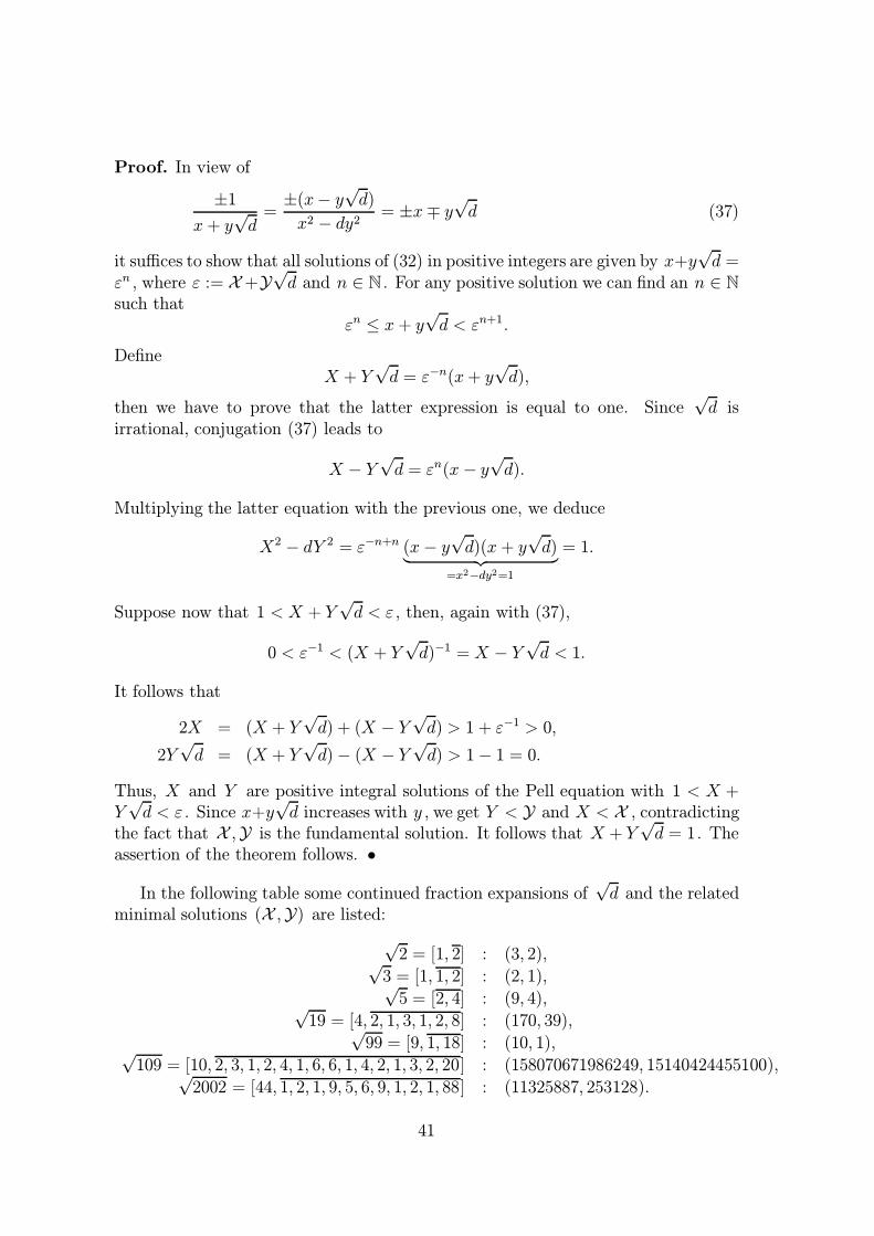
Proof. In view of

±1

x+ y√d

=±(x− y

√d)

x2 − dy2= ±x∓ y

√d (37)

it suffices to show that all solutions of (32) in positive integers are given by x+y√d =

εn , where ε := X+Y√d and n ∈ N . For any positive solution we can find an n ∈ N

such thatεn ≤ x+ y

√d < εn+1.

DefineX + Y

√d = ε−n(x+ y

√d),

then we have to prove that the latter expression is equal to one. Since√d is

irrational, conjugation (37) leads to

X − Y√d = εn(x− y

√d).

Multiplying the latter equation with the previous one, we deduce

X2 − dY 2 = ε−n+n (x− y√d)(x+ y

√d)︸ ︷︷ ︸

=x2−dy2=1

= 1.

Suppose now that 1 < X + Y√d < ε , then, again with (37),

0 < ε−1 < (X + Y√d)−1 = X − Y

√d < 1.

It follows that

2X = (X + Y√d) + (X − Y

√d) > 1 + ε−1 > 0,

2Y√d = (X + Y

√d)− (X − Y

√d) > 1− 1 = 0.

Thus, X and Y are positive integral solutions of the Pell equation with 1 < X +Y√d < ε . Since x+y

√d increases with y , we get Y < Y and X < X , contradicting

the fact that X ,Y is the fundamental solution. It follows that X + Y√d = 1. The

assertion of the theorem follows. •

In the following table some continued fraction expansions of√d and the related

minimal solutions (X ,Y) are listed:

√2 = [1, 2] : (3, 2),√

3 = [1, 1, 2] : (2, 1),√5 = [2, 4] : (9, 4),√

19 = [4, 2, 1, 3, 1, 2, 8] : (170, 39),√99 = [9, 1, 18] : (10, 1),√

109 = [10, 2, 3, 1, 2, 4, 1, 6, 6, 1, 4, 2, 1, 3, 2, 20] : (158070671986249, 15140424455100),√2002 = [44, 1, 2, 1, 9, 5, 6, 9, 1, 2, 1, 88] : (11325887, 253128).

41

It can be shown that the minimal solution of the Pell equation related tothe cattle problem leads to an herd consisting of N = 77602 . . . 81800 manybulls and cows, where the number N has 206545 digits. On the webpagewww.bioinfo.rpi.edu/ zukerm/cgi− bin/dq.html the interested (lazy?) reader can findan online Pell solver. The size of the minimal solution of the Pell equation behavesquite unregularly by increasing d . This is an interesting topic related to severaldeep and important questions; for example, the class number problem.

Another related topic are polynomial Pell equations. For instance, let d = 1or d = ±2, then in [36] it is proved that the sequences of polynomials given byP0 = 1, Q0 = 0 and, for n ∈ N ,

Pn(X) =(

2

dX2 + 1

)Pn−1(X) +

2

dX(X2 + d)Qn−1(X),

Qn(X) =2

dXPn−1(X) +

(2

dX2 + 1

)Qn−1(X)

satisfy the polynomial equation P (X)2− (X2 +d)Q(X)2 = 1 , and that these are (upto the sign) all solution of the latter equation. However, it is an open problem todetermine the polynomials D for which the polynomial Pell equation P 2−D·Q2 = 1has non-trivial solutions.

Since it has nothing to do with Pell or the Pell equation, we conclude withanother interesting infinite representation due to Ramanujan:

Exercise 25 Prove that

n+ 1 =

√1 + n

√1 + (n+ 1)

√1 + (n + 2)

√. . . for n ∈ N.

10 Factorization with continued fractions

We are living in times with exponentially increasing electronic information exchange.This led to so-called public key-cryptosystems which mainly rely on so-called one-way functions, i.e. a simple operation which has an inverse that can hardly becomputed. It is simple to multiply integers but, conversely, it is rather difficultto find the prime factorization of a given large integer; it is conjectured that thefactorization of integers is an NP-hard problem, i.e., roughly speaking, there existsno fast algorithm. In the sequel we follow [10] and [28].

One of the first modern factorization methods is the Continued fractionmethod CFRAC due to Lehmer and Powers. This algorithm was first implementedby Brillhart and Morrison in 1970. As a proof for the power of it they computed thefactorization of the 38-digit seventh Fermat number F7 := 227

+1; for the currentknowledge on Fermat numbers see www.prothsearch.net/fermat.html]Prime. In thefollowing years CFRAC became the main factoring algorithm in practice; actuallyit was the first algorithm of expected sub-exponential running time. CFRAC reliesin the main part on some ideas due to Fermat, Legendre and Kraitchik. Suppose

42

that we are interested in the prime factorization of a large integer N . If there areintegers x, y for which

x2 ≡ y2 mod N and x 6≡ ±y mod N,

then the greatest common divisor (N, x + y) is a non-trivial factor of N . Thisfollows immediately from the identity x2 − y2 = (x− y)(x+ y) . To look randomlyfor pairs of squares which satisfy these conditions seems to be hopeless. The mainidea is to collect sufficiently many squares which lie modN in the same residueclass, such that certain combinations among them lead to non-trivial divisors of N .More precisely, having sufficiently many congruences

x2j ≡ (−1)ε0j`

ε1j1 `

ε2j2 · . . . · `

εmjm mod N,

where the `k are small prime numbers and the εkj are the related exponents, byGaussian elimination modulo 2 we may hope to find a relation of the form∑

j≤n

δj(ε0j, . . . , εmj) ≡ (0, . . . , 0) mod 2, (38)

where δj ∈ {0, 1} . Then, setting

x =∏j≤n

xδjj and y = (−1)ν0`ν1

1 `ν22 · . . .· `

νmm , (39)

where∑j≤n δj(ε0j, . . . , εmj) = 2(ν0, ν1, . . . , νm) , we get x2 ≡ y2 mod N . This splits

N if x 6≡ ±y mod N . The set of prime numbers ` which are choosen to find thecongruences in addition with −1 is called factor basis.

Whereas in the Quadratic sieve factoring algorithm the squares x2j are generated

by the nearest integers to√N the continued fraction algorithm works with the

numerators of the convergents to√N . This idea becomes more transparent in the

algorithm

CFRACFor j = 0, 1, 2, . . . successively:1. Compute the j th convergent pj

qjof the continued fraction expansion to

√N .

2. Compute p2j mod N such that the absolute value is ≤ 1

2N . After doing this for

several j , look at the numbers ±p2j mod N which factor into a product of small primes.

Define your factor base B to consist of −1 , the primes which either occur in more thanone of the p2

j mod N or which occur to an even power in just one p2j mod N .

3. List all of the numbers p2j mod N which can be expressed as a product of numbers

in the factor base B . If possible, find a subset of numbers ` ’s of B for which theexponents ε according to the numbers in B sum to zero modulo two as in (38), anddefine x, y by (39). If x 6≡ ±y mod N , then (x + y,N) is a non-trivial factor ofN . If this is impossible, then compute more p2

j mod N , enlarging the factor base B ifnecessary.

43

Once the number of completely factored integers exceeds the size of the factor base,we can find a product of them which is a perfect square. With a little luck thisyields a non-trivial factor of our given number (by the observations from above).The crucial property of the values pj is, as we shall show below, that their squareshave small residues modulo N . Otherwise, CFRAC would hinge on the problem offinding an appropriate factor base B .

Theorem 23 Let α > 1 be irrational. Then the convertgents pnqn

to α satisfy theinequality

|q2nα

2 − p2n| < 2α.

In particular, if α =√N , where N ∈ N is not a perfect square, then the residue

p2n mod N which is smallest in absolute value is less than 2

√N .

Proof. In view of Theorem 11,

|q2nα

2 − p2n| = q2

n

∣∣∣∣∣α − pn

qn

∣∣∣∣∣ ·∣∣∣∣∣α +

pn

qn

∣∣∣∣∣ < q2n

qnqn+1

(α +

(α+

1

qnqn+1

)).

Thus,

|q2nα

2 − p2n| − 2α < 2α

(−1 +

qn

qn+1+

1

2αq2n+1

)< 2α

(−1 +

qn + 1

qn+1

),

which is less or equal to zero, and proves the first assertion of the theorem. Theclaim on p2

n mod N is an immediate consequence. •

Therefore, the sequence of the numerators of the convergents of√N provides

a sequence of pj ’s whose squares have small residues modN ; in fact, for that onehas even not to calculate the actual convergent in the continued fraction expansion,only the numerator pj modulo N is needed.

We illustrate CFRAC by an example. Consider N = 9073. It is easy to computethe continued fraction expansion and its convergents:

95

1,

286

3,

381

4,

10192

107,

20765

218, . . . →

√9073 = [95, 3, 1, 26, 2, . . .].

This leads to

j | 0 1 2 3 4pj mod 9073 | 95 286 381 1119 2619p2j mod 9073 | −48 139 −7 87 −27

It is not too difficult to factor the small numbers p2j mod 9073. We may choose the

factor base B = {−1, 2, 3, 7} , so that p2j mod N is a B -number for j = 0, 2, 4. The

corresponding vectors of exponents αj are

{1, 4, 1, 0}, {1, 0, 0, 1} and {1, 0, 3, 0}.

44

The sum of the first and the third adds up to zero modulo two, which yields

x = 95 · 2619 ≡ 3834 mod 9073 and y = 22 · 32 = 36.

It follows that38342 ≡ 362 mod 9073.

Since 3834 6≡ ±36 mod 9073, we see that (3834 + 36, 9073) = 43 is a divisor of9073 (the computation of greatest common divisors is easily done by the euclideanalgorithms backwards). This leads to the prime factorization 9073 = 43 · 211.

Exercise 26 Use CFRAC to factor the integers N = 17873, 25511 .

It is a well-known fact that CFRAC does not work for prime powers N = pk, k ≥ 2(which is obvious if k is even but also true for odd exponents k ). This is not a bigproblem. It is easy to check rather quickly whether a given N is a prime poweror not. However there are other examples for which CFRAC does not work. If theperiod of the continued fraction expansion of

√N is too short, then the algorithm

can produce only a small factor basis, which reduces the chances for factoring N .For instance, if N = n2 + 2, then it is easily computed that p2

j mod (n2 + 2) = 1 or= −2 (by hand or with our knowledge on the Pell equation with d = N ). This givesin the CFRAC algorithm (x+ y, n2 + 2) = n± 1 which does not divide n2 + 2 = N .A suitable refinement can be found in [54].

Having this powerful factoring algorithm in mind, we could be pessimistic aboutthe security of cryptosystems:

Three may keep a secret, if two of them are dead. Benjamin Franklin

However, in modern cryptosystems prime numbers with approximately one hundreddigits are used, whereas numbers which are the product of two such large primescannot be factored in an appropriate time by the most modern factorization algo-rithms in practice. More details on this can be found in the excellent monography[10]; for applications of continued fraction algorithms to primality tests we refer to[7].

11 Liouville’s theorem

A complex number α is called transcendental if it is not algebraic, i.e., thereexists no polynomial with rational coefficients and root α . The use of the wordtranscendental dates at least back to Leibniz who wrote in 1704 omnem rationemtranscendunt. First of all, it is not clear whether transcendental numbers exist.Using Cantor’s notion of countability we can easily find an answer.

The height H(P ) of a polynomial P with integral coefficients is defined to bethe maximum of all coefficients of P in absolute value. Let D,H be positive real

45

numbers. Then it is easily seen that there exist only finitely many polynomialsP (X) with integral coefficients for which

degP ≤ D and H(P ) ≤ H.

It follows that the set of polynomials with rational coefficients is countable. Inparticular, the set of roots of such polynomials is also a countable set. On the otherside, R is uncountable. Thus

Theorem 24 The set of algebraic numbers is countable, and the set of transcen-dental numbers is uncountable.

This shows that almost all numbers are transcendental, but, actually, we do notknow at least one transcendental number so far. This was one of the major problemsfrom 19th century mathematics. In 1844 Liouville solved the problem.

Theorem 25 For any algebraic number α of degree d > 1 there exists a positiveconstant c , depending only on α , such that∣∣∣∣∣α− p

q

∣∣∣∣∣ > c

qd

for all rationals pq

.

Proof. Denote by P (X) the minimal polynomial of α . Then, by the mean-valuetheorem,

−P

(p

q

)= P (α)︸ ︷︷ ︸

=0

−P

(p

q

)=

(α −

p

q

)P ′(ξ)

for some ξ lying in between pq

and α . Obviously, we may assume that∣∣∣α− p

q

∣∣∣ < 1.

Then |ξ| < 1 + |α| and hence |P ′(ξ)| < 1c

for some positive c . It follows that∣∣∣∣∣α− p

q

∣∣∣∣∣ > c

∣∣∣∣∣P(p

q

)∣∣∣∣∣ .Since P (X) is irreducible, it turns out that p

qis not a zero of P (X) , and hence

∣∣∣∣∣qdP(p

q

)∣∣∣∣∣ ≥ 1,

which proves the theorem. •

The proof even provides a value for the constant c in terms of the height. Theheight H(α) of an algebraic number α is defined by H(α) = H(Pα) , where Pα isthe minimal polynomial of α .

46

Exercise 27 Prove that one can take

c =1

d2(1 + |α|)d−1H(α)

in Liouville’s theorem.

Liouville’s theorem shows that algebraic numbers cannot be approximated toogood by rationals. Consequently, a real number which can be better approximated hasto be transcendental! This is easily seen as follows: if we assume that α = [a0, a1, . . .]is algebraic of degree d , then we have in view of equation (29) and Liouville’s theoremthe inequality

c

qdn<

∣∣∣∣∣α − pn

qn

∣∣∣∣∣ ≤ 1

an+1q2n

,

resp.

can+1 < qd−2n , (40)

where the positive constant c depends only on α . If d = 2, the case of quadraticirrationals α , we see what we already know, namely that the sequence of partialdenominators of α is bounded. But whenever

lim infn→∞

an+1

qn=∞,

we may find for any positive δ infinitely many convergents to α for which an+1 ≥ qδn ,contradicting (40). Hence, such an α cannot be algebraic. For instance, the realnumber α = [1, 101!, 102!, 103!, . . .] is transcendental. However, it is more convenientto deal with series.

Exercise 28 Show that

α =∞∑n=1

10−n! = 0.11000 10000 . . .

is transcendental.In Exercise 5 we have proved that α is irrational.

A real number α is a Liouville number if for each positive integers m thereexist numbers am, bm such that

0 <∣∣∣∣α − am

bm

∣∣∣∣ < 1

bmmand bm > 1.

In view of Liouville’s theorem it is easy to show, by the same reasoning as above,that every Liouville number is transcendental. It should be noted that Liouvillewrote in his underlying paper

47

Je crois me souvenir qu’on trouve un theoreme de ce genre dans une lettre deGoldbach a Euler; mais je ne sache pas que la demonstration en ait jamais ete

donnee. (cf [8])

Liouville numbers are very interesting. One can prove that Liouville numbers forman uncountable set of Lebesgue measure zero. On the other side, Erdos [15] showedthat every real number can be written as a sum, resp. a product, of two Liouvillenumbers; for this and other related results see [41].

12 The transcendence of e and π

The Liouville numbers from the previous paragraph look somehow artifical. It ismuch more difficult to decide whether a given number is transcendental or algebraic.The first and path-breaking result in this direction was proved by Hermite in 1873.

Theorem 26 e is transcendental.

Niven’s proof for the irrationality of π (see Theorem 2) is based on Hermite’s prooffor the transcendence of e

Proof. Define

I(t) =∫ t

0et−xf(x) dx

for t ≥ 0, where f is a real polynomial of degree m . Integration by parts showsthat

I(t) = −et−xf(x)

∣∣∣∣∣t

x=0

+∫ t

0et−xf ′(x) dx = et

m∑j=0

f (j)(0)−m∑j=0

f (j)(t). (41)

Denote by F the polynomial obtained from f by replacing each coefficient with itsabsolute value. Then

|I(t)| ≤∫ t

0et−x|f(x)|dx ≤ tetF (t). (42)

Suppose now that e is algebraic, then there exists a polynomial P with integralcoefficients ak and leading coefficient ad 6= 0 for which

d∑k=0

akek = 0.

Without loss of generality we may assume that P is the minimal polynomial of e .For a large prime p set

f(x) = xp−1d∏k=1

(x− k)p;

48

the degree of f is equal to m = (d+ 1)p− 1. We shall consider

J :=d∑k=0

akI(k).

In view of (41)

J =d∑k=0

ak

ek m∑j=0

f (j)(0)−m∑j=0

f (j)(k)

= −m∑j=0

d∑k=0

akf(j)(k). (43)

For 1 ≤ k ≤ d we have f (j)(k) = 0 for j < p . Further, if j ≥ p , then

f (j)(k) =

(j

p

)p! · g(j−p)(k) , where g(x) :=

f(x)

(x− k)p.

Thus, for all j , f (j)(k) is an integer divisible by p! . Similarly, f (j)(0) = 0 forj < p− 1, and further, for j ≥ p− 1,

f (j)(0) =

(j

p− 1

)(p− 1)! · h(j−p+1)(0) , where h(x) :=

f(x)

xp−1.

It follows that h(j)(0) is an integer divisible by p for j > 0, and h(0) = (−1)dp(d!)p .Consequently, for j 6= p− 1, f (j)(0) is also an integer divisible by p! , and f (p−1)(0)is an integer divisible by (p− 1)! but not by p for p > d . Therefore, let p > d . Itfollows that J is a non-zero integer (by the first identity in (43)) which is divisibleby (p− 1)! (by the second identity in (43)). Hence, |J | ≥ (p − 1)! . On the otherhand, the trivial bound F (k) ≤ (2d)m implies via the estimate (42)

|J | ≤d∑k=0

|ak|kekF (k) ≤ H(e)d(d + 1)(2d)(d+1)p−1 ≤ cp,

where c is a constant independent of p . Thus,

(p− 1)! ≤ |J | ≤ cp,

which is impossible for sufficiently large p . This contradiction shows that e cannotbe algebraic. •

Following Hermite’s ideas Lindemann succeeded in 1882 in showing

Theorem 27 π is transcendental.

Proof. Suppose that π is algebraic. It follows that also α := iπ is algebraic, say ofdegree d . Denote the conjugates of α by α1 = α, α2, . . . , αd . From Euler’s identityexp(iπ) = −1 it follows that

(1 + eα1︸ ︷︷ ︸=0

)(1 + eα2) · . . . · (1 + eαd) = 0.

49

The product on the left hand side can be written as a sum of 2d terms e% , where

% = δ1α1 + . . .+ δdαd,

and δj = 0 or 1. Now we assume that precisely n of the numbers % are non-zeroand denote them by β1, . . . , βn . It follows that

q + eβ1 + . . .+ eβn = 0 , where q := 2d − n.

Now we shall proceed as in the previous proof and compare estimates for

H :=n∑k=1

I(βk),

where I(t) is defined by (41) with

f(x) = `npxp−1n∏k=1

(x− βk)p,

` is the leading coeeficient of the minimal polynomial of α and p again denotes alarge prime number, chosen later. We obtain

H = −qm∑j=0

f (j)(0)−m∑j=0

n∑k=1

f (j)(βk),

where m = (n + 1)p − 1. Now the sum over k is a symmetric polynomial in`β1, . . . , `βn with integral coefficients. From the fundamental theorem on symmetricfunctions in addition with the observation that each elementary symmetric functionin `β1, . . . , `βn is also an elementary symmetric function in the 2d numbers `% itfollows that the sum over k is an integer. Since f (j)(βk) = 0 for j < p the sum inquestion is divisible by p! . Further, f (j)(0) is an integer divisible by p! if j 6= p−1,and

f (p−1)(0) = (p− 1)!(−`)np(β1 · . . . · βn)p,

which is an integer divisible by (p− 1)! but not by p! when p is sufficiently large.Thus, |H| ≥ (p− 1)! if p > q . But on the other side, (42) implies the upper bound

|H| ≤n∑k=1

|βk|F (|βk|) ≤ cp

for some constant c independent on p . As in the previous proof, this gives thecontradiction. π is not algebraic. •

As an important consequence of Lindemann’s theorem one obtains a negativeanswer to an old and famous problem of the ancient Greek: it is impossible to squarea circle by using only ruler and compass. This follows from the obvious fact thatall points capable of construction are defined by intersection of lines and circles,

50

and thus have only algebraic distances one from another; but on the other side,√π is transcendental. Actually, Lindemann proved a stronger result, namely: for

any distinct algebraic numbers α1, . . . , αn and any non-vanishing algebraic numbersβ1, . . . , βn ,

β1eα1 + . . . + βne

αn 6= 0.

The transcendence of e follows immediately, the one of π by Euler’s identity.

Exercise 29 Using Lindemann’s theorem prove the transcendence of the trigono-metric functions sinα, cosα and tanα for all non-zero algebraic α .

There are many open problems in transcendental number theory. It is yet un-proved whether e and π are algebraically independent or, to be more concrete, aree+ π and e · π both transcendental?

Exercise 30 Show that at least one of the numbers e+ π, e · π is transcendental.

In his seventh problem Hilbert asked for a proof that αβ is transcendental when-ever α 6= 0, 1 and β are algebraic irrationals. In 1934 Gel’fond and Schneider(independently) succeeded in showing this deep result. A generalization was ob-tained by Alan Baker’s celebrated estimates for linear forms in logarithms for whichhe was awarded with the Fields medal at the International Congress in Moscow1966. For instance, he proved the transcendence of

exp(β0)αβ11 · . . . · α

βnn

and that of any non-vanishing linear form

β1 logα1 + . . . + βn logαn,

where the αj and βj denote non-zero algebraic numbers. For more details and aproof see [3], [45] or [8]

13 The theorem of Roth

It is natural to ask for stronger versions of Liouville’s theorem. Only a slight im-provement would imply the finiteness of integral solutions of certain important dio-phantine equations; a theme to which we shall return in a later section. Supposethat α is an algebraic number of degree d , then we might ask for exponents τ (d)such that there exists a positive constant c , depending only on α , such that for allrationals p

q∣∣∣∣∣α− p

q

∣∣∣∣∣ > c

qτ (d). (44)

The first refinement to Liouville’s bound τ (d) = d was made by Thue who showedin 1909 that τ (d) > 1

2d + 1. In 1921 Siegel obtained τ (d) > 2

√d (it should be

noted that Siegel became professor in Frankfurt short after this discovery), and thefamous physiscist Dyson proved in 1947 that τ (d) >

√2d . Finally, Roth proved in

1955 that τ (d) can be chosen independently of the algebraic degree d .

51

Theorem 28 Let α be an algebraic number of degree d ≥ 2 and let ε > 0. Thenthere exist only finitely many rational solutions p

qto the inequality∣∣∣∣∣α − p

q

∣∣∣∣∣ < 1

q2+ε.

This shows that one can take any τ = τ (d) > 2 in (44); actually this is equivalentto Theorem 28. Consequently, algebraic numbers are approximable of order κ = 2but not better. In view of Dirichlet’s approximation theorem Roth’s theorem is bestpossible with respect to the exponent 2. It might be possible that the ε -quantitycan be sharpened. Lang conjectured that for α of degree d ≥ 3,∣∣∣∣∣α − p

q

∣∣∣∣∣ > c

q2(log q)κ

has only finitely many solutions if κ is a constant > 1. Roth got the Fields medalfor his celebrated theorem during the International congress of mathematicians atEdinburgh in 1958. Unfortunately, Roth’s theorem is ineffective. The method ofproof does not provide an algorithm to determine the set of solutions. However, inparticular cases it is possible to obtain upper bounds for the number of solutions(but this is a topic to which we will return later). A multidimensional generalizationof Roth’s theorem is the celebrated subspace theorem of W.M. Schmidt; a nice surveyon this modern field of research is [43].

We can only sketch the idea of Roth’s ingenious proof; the technical details aretoo complicated but the main ingredients become visible. We will follow [42] butfirst we review Liouville’s idea. The proof of Theorem 25 depends mainly on

• the construction of a polynomial P (X) with integral coefficients that vanishes

at α and for which P(pq

)is small in terms of

∣∣∣α − pq

∣∣∣ , and

• the fact that P(pq

)cannot be too small as a function of q .

Thue’s ingenious contribution was to introduce polynomials in two variables whichprovides more freedom in the search for suitable polynomials. Before Roth it wasalready known that any progress would demand the use of polynomials in morethan two variables. We start to formulate some properties which a polynomialshould have. Suppose that for 1 ≤ n ≤ m the rational approximations pn

qnto α

satisfy ∣∣∣∣∣α− pn

qn

∣∣∣∣∣ < 1

qτn, (45)

where τ is some positive real number. Let P (X1, . . . , Xm) be a polynomial withintegral coefficients, of degree at most rn in Xn for each n . It follows that∣∣∣∣∣P

(p1

q1

, . . . ,pm

qm

)∣∣∣∣∣ ≥ 1

Q, where Q := qr11 · . . . · q

rmm , (46)

52

provided that

P

(p1

q1, . . . ,

pm

qm

)6= 0. (47)

Let the Taylor expansion of P(p1

q1, . . . , pm

qm

)in powers of pn

qn− α be

∑j1

. . .∑jm

cj1,...,jm

(p1

q1

− α

)j1· . . . ·

(pm

qm− α

)jm.

Suppose now that P has in additon to (47) the properties that for small positive δ ,∑j1

. . .∑jm

|cj1,...,jm| < Qδ, (48)

and cj1,...,jm = 0 for all j1, . . . , jm satisfying

qj11 · . . . · qjmm ≤ Q∆, (49)

where ∆ > 0. Taking into account (45) we have for each term in the Taylor serieswith a non-zero coefficient∣∣∣∣∣p1

q1− α

∣∣∣∣∣j1

· . . . ·

∣∣∣∣∣pmqm − α∣∣∣∣∣jm

<1

(qj11 · . . . · qjmm )τ

≤1

Qτ∆.

Consequently, ∣∣∣∣∣P(p1

q1, . . . ,

pm

qm

)∣∣∣∣∣ < 1

Qτ∆−δ.

In view of (46) it follows that

τ <1 + δ

∆. (50)

In order to prove Theorem 28 we shall establish the existence of a polynomial Pwhich satisfies the conditions (47), (48) and (49) with ∆ near to 1

2as δ → 0. For this

purpose it is necessary to take the number of variables m large and to choose suitableapproximations pj

qj(actually, taking m = 2 leads only to an estimate τ < c

√d).

In some sense, the question of good lower bounds for rational approximations toalgebraic numbers is transformed to an approximation problem for polynomials inseveral variables; the use of many variables allows to put certain restrictions on thepolynomial in question. We shall go a bit more into the details that at least theestimate τ > 2 becomes lucid.

The argument is indirect. We suppose that τ > 2. If there are infinitely manyrationals satisfying (45), then we can find a subsequence p1

q1, . . . , pm

qmfor which

log qnlog qn−1

>1

ε

53

with some positive ε and large q1 . Then we may choose positive integers rn satis-fying

qr11 ≤ qrnn < q

r1(1+ ε10

)1 .

Consequently, qmr11 ≤ Q < qmr1(1+δ)1 . Then condition (49) takes the form that the

Taylor coefficients cj1,...,jm vanish for all j1, . . . , jm with

j1

r1+ . . .+

jm

rm< m∆ + δ. (51)

The next step is to construct a polynomial P ∗ that satisfies conditions (48) and (49)only. This is done following an argument of Siegel which bases on Dirichlet’s pigeon-hole principle. We put B = qr11 and consider the set of polynomials W (X1, . . . , Xm)of degree at most rn in Xn , and having integral coefficients, each of modulus lessthan B . We shall try to find two distinct polynomials W1,W2 such that their deriv-atives of order j1, . . . , jm are equal whenever X1 = . . . = Xm = α , for all j1, . . . , jmsatisfying (51). Any such derivative is of the form

a0 + a1α + . . .+ an−1αn,

where the aj are integers. It can be shown that the number of possibilities for aderivative for given j1, . . . , jm is < Bn(1+3ε) , whereas the number of polynomials Wis about Br , where r = (r1 +1) · . . .·(rm+1). Hence, the number of possible distinctsets of derivatives provided that the number of sets j1, . . . , jm satisfying (51), andwith no jk exceeding the corresponding rk , is less than about r

n(1+3ε). The number

of integer points (j1, . . . , jm) in the region defined by the above conditions can beshown to be less that 2r

3nif ∆ is chosen by

m∆ + δ =1

2m− 3nm

12 .

A more detailed analysis shows that we may assume that δ tends with ε to zero asm→∞ . Thus we obtain

∆ =1

2−

δ

m−

3n

m12

.

This shows that the number of variables m has to be chosen large to give a value ofτ nearby 2 in (50). This choice yields the existence of such polynomials W1,W2 .Now the polynomial P ∗ = W1 −W2 satisfies condition (49), and it can be shownby some estimation process that it also satisfies (48). We cannot expect that P ∗

satisfies also condition (47). Actually, the construction of a polynomial P out of P ∗

which satisfies (47) is the most difficult aspect in Roth’s theorem (Roth’s lemma).Unfortunately, this is beyond the scope of this course; for details see the excellent[44], [45] and [60]. The final contradiction in Roth’s proof is that for sufficientlylarge m we can find a ∆ as close to 1

2as we please for which the right hand side of

(50) exceeds any given τ > 2.

There is an interesting correspondence to complex analysis due to Vojta. It isconjectured that the exponent 2 in Roth’s theorem is the same number 2 which

54

occurs in the defect relation in Nevanlinna’s value-distribution theory or, roughlyspeaking, there seems to be a bridge between the approximation theories for numbersand for functions; for details see [59].

Roth’s theorem has many important implications. For instance, following thelines of Liouville’s proof of the transcendence of Liouville numbers, one can obtaina transcendence criterion for continued fractions.

Exercise 31 Let ε > 0 and suppose that α = [a0, a1, . . .] is an irrational numberwhich has an infinity of partial quotients satisfying an+1 ≥ qεn , where qn is thedenominator of the n-th convergent to α . Prove that α is transcendental.

Another interesting consequence is Everett’s attack on Fermat’s last theorem.The main result of [16] states that if p is a fixed odd prime and ν is a fixed positiveinteger, then there are at most finitely many pairs of coprime integers x, y on theline y = x+ν such that xp+yp is the p-th power of an integer, whereas in the casep = 2 there are an infinitude of such pairs x, y for which x2 + y2 is a square; thefirst result follows tricky but elementary from Theorem 28, and the second one fromthe theory of Pell equations. The most important implication of Roth’s theorem isto find in the theory of cubic curves.

14 Thue equations

During his stay in London the ingenious Indian mathematician Ramanujan spendseveral weeks in hospital. Once his colleague Hardy came to visit and remarkedthat he had come in taxicab number 1729, which is surely a rather dull number.Ramanujan replied immediately that this is not true; 1729 is rather interesting sinceit is the smallest integer expressible as a sum of two cubes in two different ways:

1729 = 13 + 123 = 93 + 103.

This can be seen as follows. Since

(X + Y ) · (X2 −XY + Y 2) = X3 + Y 3 = 1729 = 7 · 13 · 19,

we have to consider all possible factorizations 1729 = A ·B and solve

A = X + Y and B = X2 −XY + Y 2. (52)

The substitution Y = A−X leads to the quadratic equation

3X2 − 3AX +A2 −B = 0,

so that we only have to check if

1

6(3A±

√12B − 3A2)

is an integer. This yields the two pairs A = 13, B = 133 and A = 19, 91 whichcorrespond to the above given representations. We leave it to the reader to checkthat all integers m < 1729 have at most one representation as a sum of two cubes.

55

Exercise 32 Find all integral solutions to the equation X3 + Y 3 = 403 . What canyou say about the set of solutions of X3 − Y 3 = m with m = 0 and m = 1729 ,respectively?

It is one thing to know that a certain diophantine equation has only finitely manysolutions. However, for a complete list of all solutions one needs to have knowledgeon their size.

Theorem 29 Let m be a positive integer. Then every solution to the equation

X3 + Y 3 = m (53)

in integers x, y satisfies the inequality

max{|x|, |y|} ≤ 2

√m

3.

Proof. By the above reasoning each integral solution x, y satisfies (52) for somefactorization m = A ·B . Hence

m ≥ |B| = |x2 − xy + y2| =3

4x2 +

(1

2x− y

)2

≥3

4x2,

which gives the bound for x ; since the equation is symmetric with respect to X andY the same estimate holds for y as well. This proves the theorem. •

There is a big difference between the sets of rational numbers and of integers withrespect to diophantine equations. We have shown that equation (53) has only finitelymany integral solutions. On the contrary it can be shown that, for example, theequation

X3 + Y 3 = 9

has infinitely many rational solutions. The transformation

X 7→12

X + Yand Y 7→ 12

X − Y

X + Y

provides a one-to-one correspondence between the rational solutions of the previousequation and the rational points on the curve

Y 2 = X3 − 48;

the latter equation defines a so-called elliptic curve (this is not an ellipse butit is related to such objects). The theory of elliptic curves tells us that there areinfinitely many rational solutions. The interested reader can find more details inthe excellent monography [51]. A more simple but from a geometric point of viewdifferent example is the unit circle.

Analyzing (53) was rather simple since our diophantine equation was related toa reducible polynomial. If we have instead an irreducible polynomial, as for exampleX3 + 2Y 3 = m , the situation is much more difficult. The first remarkable result forsuch equations was found by Thue in 1909.

56

Theorem 30 Let a, b, c be non-zero integers. Then the equation

aX3 + bY 3 = c (54)

has only finitely many solutions in integers.

Proof. If x, y ∈ Z is a solution to (54) then X = ax, Y = y is a solution toX3 + a2bY 3 = a2c . Thus it is enough to prove the theorem with a = 1. Further,since we may replace y by −y and/or b by −b in (54) if necessary, it is sufficientto consider the equation

X3 − bY 3 = c, (55)

where b, c are positive integers. The factorization method which we used in theproof of Theorem 29 worked very well. This observation motivates to have a lookon the factorization

X3 − bY 3 = (X − βY ) · (X2 + βXY + β2Y 2) with β =3√

3. (56)

If b is a perfect cube β , the latter identity is a factorization over the integers andwe can factor c and proceed as above. If b is not a perfect cube, we need a differentidea. Then we argue as Euler did in case of the Pell equation. If x, y ∈ N is a largesolution of (55), then the first factor on the right hand side of (56) must have smallmodulus. This follows from the estimate

x2 + βxy + β2y2 =(x+

1

2βy)2

+3

4(βy)2 ≥

3

4β2y2, (57)

which implies via (56)

c = x3 − by3 = |x− βy| · |x2 + βxy + β2y2| ≥3

4β2y2 · |x− βy|.

This gives∣∣∣∣∣β − x

y

∣∣∣∣∣ ≤ 4c

3β2y3. (58)

In view of Roth’s theorem it follows that the latter inequality can have only finitelymany solutions x

ywhich implies the assertion of the theorem. •

Note that also Thue’s estimate τ (3) > 52

in (44) is sufficient as well (Thue didnot have Roth’s bound) but not Liouville’s τ (3) = 3. Theorem 30 can easily beextended to equations of higher degree, so-called Thue equations.

Exercise 33 Let P (X, Y ) be an irreducible binary form with integral coefficients ofdegree at least three and let m be any integer. Show that the equation P (X, Y ) = mhas only finitely many solutions in integers. [Hint: instead of (57) work with a mean-value

argument as in the proof of Liouville’s theorem.]

57

In view of Exercise 32 the condition on the irreducibility of P in the exercise aboveis necessary.

The approach via diophantine approximations has its limitations. Althoughthe set of integral solutions is finite Thue’s argument does not enable to give acomplete list of solutions or indeed to determine whether the equation is soluble (weshall discuss this question in the following section). This follows from the fact thatRoth’s theorem is ineffective. In particular cases - here we do not mean trivial casesas settled in Theorem 29 - one can succeed by Baker’s estimates for linear forms inlogarithms. For example, Baker [2] obtained the estimate∣∣∣∣∣pq − 3

√2

∣∣∣∣∣ ≥ 10−6

q2.9955,

valid for all rationals pq

. The exponent is larger than Roth’s exponent 2 + ε but

the implicit constant is absolute. Combining this with (58) shows that any integersolution x, y to

X3 − 2Y 3 = c,

where c is a positive integer, satisfies the estimate

|y| ≤ 101317c223.

This is a large bound, but at least it only grows like a power of c .Meanwhile more than Thue’s theroem is known. The more general equation

aX3 + bX2Y + cXY 2 + dY 3 + eX2 + fXY + gY 2 + hX + iY + j = 0

describes a cubic curve. In his PhD thesis Siegel proved that a non-singular cubiccurve with integral coefficients has only finitely many points with integral coordinates;geometrically speaking, a point is called singular if it is a double point. It is easilyseen that linear or quadratic equations can have an infinitude of solutions in integers(e.g. Pell’s equation). Furthermore, by Faltings’ celebrated proof of the Mordellconjecture we know that any curve of genus ≥ 2 has only finitely many rationalpoints. Note that Faltings was awarded with a Fields medal at the InternationalCongress of mathematicians in Berkeley 1986, following the footprints of Roth andBaker. We do not explain here what the topological notion genus means but notethat this extends the class of homogeneous equations in two variables which Thuecould handle and covers, for example, Fermat’s last theorem (1). For a nicely writtenoverview see the last chapter of [25].

15 The abc-conjecture

There is no complete theory for the variety of diophantine equations known. And iteven seems that there exists nothing like that. In his tenth problem Hilbert asked ifthere exists a universal algorithm which can determine whether a given polynomial

58

diophantine equation with integral coefficients has a solution in integers. In 1970Matjasevic gave a negative answer; for the most simple proof see [26]. Besideshe proved that the set of prime numbers is diophantine, where a set A is calleddiophantine if there exists a polynomial P (X1, . . . , Xn) with integral coefficientssuch that the equation P (X1, . . . , Xn−1, a) = 0 has integral solutions if and only ifa ∈ A . On the other side, Putnam showed that a set is diophantine if and onlyif it coincides with the set of positive values of a suitable polynomial taken at thenonnegative integers. Consequently, there exists a polynomial g(X1, . . . , Xn) whosepositive values at integers xj ≥ 0 are primes, and every prime can be represented thisway. Surprisingly, it is even possible to find such polynomials; here is an exampledue to Jones, Sato, Wada and Wiens of degree 25 in the 26 variables a, b, c, . . . , z :

(k + 2) ·{

1− [wz + h+ j − q]2 − [(gk + 2g + k + 1)(h + j) + h− z]2

−[2n+ p + q + z − e]2 − [16(k + 1)3(k + 2)(n− 1)2 + 1− f2]2

−[e3(e+ 2)(a+ 1)2 + 1− o2]2 − [(a2− 1)y2 + 1− x2]2

−[16r2y4(a2 − 1) + 1− u2]2 − [((a+ u2(u2 − a))2 − 1)(n+ 4dy)2

+1− (x− cu)2]2 − [n+ `+ v − y]2

−[(a2− 1)`2 + 1−m2]2 − [ai+ k + 1− `− i]2

−[p+ `(a − n − 1) + b(2an+ 2a− n2 − 2n − 2)−m]2

−[q+ y(a− p− 1) + s(2ap + 2a− p2 − 2p− 2) − x]2

−[z + p`(a− p) + t(2ap− p2 − 1)− pm]2}

(cf. [40]). It is not known which is the minimum possible number of variables is(clearly, it is larger than one), and it is also not known what the minimal degree is.With regard to Godel’s incompleteness theorem we finally note another remarkableconsequence: for any given axiomization there exists a diophantine equation withoutintegral solutions (probably in three variables only) which cannot be proved in thisaxiomatic setting.

Diophantine equations are a rather difficult topic. Of course, in special cases onemight possibly succeed, sometimes even with elementary arguments.

Exercise 34 Prove that x = y = z = 0 is the only integral solution of the equation

X3 + 2Y 3 + 4Z3 − 34XY Z = 0.

[Hint: use Fermat’s method of descent, i.e. construct to a given (minimal) solution in positive

integers a smaller one.]

In particular cases it is much easier if we ask for a diophantine theory for poly-nomial equations (very often in number theory the function field cases are betterto handle). Let n(P ) denote the number of distinct complex zeros of a polynomialP (which does not vanish identically). Recall that polynomials are said to be co-prime if they do not share any of their linear factors, resp. if they have distinct

59

roots. Stothers [58] and Mason [33] (independently) proved in the eighties of thelast century the following surprising result.

Theorem 31 Let a, b, c be coprime polynomials over C , not all constant. If

a+ b = c,

thenmax{deg a, deg b, deg c} < n(abc).

Proof. In view of the identity between the polynomials they are pairwise coprime,i.e., their zeros are pairwise distinct. By the fundamental theorem of algebra let

a = Ada∏j=1

(X − αj)aj , b = B

db∏k=1

(X − βk)bk and c = C

dc∏l=1

(X − γl)cl ,

where A,B,C are complex numbers, da, db, dc and aj, bk, cl are nonnegative inte-gers, and the αj, βk, γl are the distinct complex zeros of a, b and c , respectively. Forlater use we note the partial fraction decomposition of the logarithmic derivative

(log a)′ =da∑j=1

aj

X − αj,

where the derivative is taken with respect to X ; obviously, analogous formulas holdfor b and c , respectively. Without loss of generality we may assume that a hasmaximal degree; clearly, deg a ≥ 1. Setting F = a/c and G = b/c we obtainF +G− 1 = 0. This implies F ′ +G′ = 0 and

a

b=F

G= −

G′/G

F ′/F.

We compute

F ′

F= (logF )′ = (log a)′ − (log c)′ =

da∑j=1

aj

X − αj−

dc∑l=1

cl

X − γl,

and a similar formula holds for G′/G as well. This yields

a

b= −

db∑k=1

bk

X − βk−

dc∑l=1

cl

X − γlda∑j=1

aj

X − αj−

dc∑l=1

cl

X − γl

.

Multiplying both the denominator and the numerator with

K :=da∏j=1

(X − αj) ·db∏k=1

(X − βk) ·dc∏l=1

(X − γl),

60

leads to the representationA

B=a · K

b · K=a

b,

where A,B are polynomials, both having degree < da+db+dc = n(abc) (termwise).Since a and b are coprime, and since polynomials over the complex numbers factoruniquely into irreducible (even in linear) factors, it follows that deg a < n(abc) . Thetheorem is proved.

A slightly alternative proof relies on the Riemann-Hurwitz formula from Algebraicgeometry. This idea of Silverman is outlined in [19] (which is also an excellent surveyon the abc -conjecture). An immediate and interesting consequence of Theorem 31is Fermat’s last theorem for polynomials. Let n > 2 and suppose that we havepolynomials x, y, z , not all constant, with

xn + yn = zn.

Without loss of generality we may assume that x, y, z are coprime and that x hasmaximal degree. Put a = xn, b = yn and c = zn . Since the distinct zeros ofabc = (xyz)n coincide with the distinct zeros of xyz , application of Theorem 31yields

ndeg x = deg a < n(abc) = n(xyz) ≤ deg xyz ≤ 3 deg x.

This proves that all polynomial solutions of the Fermat equation (1) with exponentn ≥ 3 are trivial, which here means that they are equal up to constant factors. Thecondition on the exponent is necessary as the example

(2X)2 + (X2 − 1)2 = (X2 + 1)2

shows; this should be compared with Exercise 1. It is remarkable that Fermat’slast theorem for polynomials coincides with Fermat’s last theorem for integers withrespect to the exponents! What can we learn out of this similarity?

For another interesting application recall that, given a polynomial D , it is un-known how to determine whether the Pell equation P 2 −DQ2 = 1 has polynomialsolutions P,Q or not (see section 9). Taking into account Theorem 31 it can beshown that if the number of distinct zeros of D is less than 1

2degD , then the

equation P 2 −D ·Q2 = 1 is unsolvable. For this and more see [56].One approach to solve the lack of having a general approach towards a theory of

diophantine equations is posing a general conjecture. First attempts were made byOesterle and in refined form by Masser soon after Theorem 31 appeared. Inspiredby the above example of Fermat’s last theorem one has to think about the correcttranslation of Theorem 31. By the fundamental theorem of algebra each polynomialover C splits into linear factors. So the degree of a polynomial is nothing else thanthe number of linear factors, and the distinct zeros correspond one-to-one to thedistinct linear factors. The size of a number is measured by the absolute value andthe irreducible factors of an integer are its prime factors. This dictionary is simple

61

and sufficient. The most common version of the abc-conjecture states that if a, b, care coprime integers which satisfy

a+ b = c,

then, for any ε > 0,

max{|a|, |b|, |c|} ≤ C(ε)

∏p|abc

p

1+ε

,

where C(ε) is a constant depending only on ε . The appearing product is calledsquarefree kernel. Unfortunately, the appearance of the ε and the related im-plicit constant are necessary as we shall explain now. Let m be a positive integer.Fermat’s little theorem from elementary number theory states that if a and n andare coprime integers, then

aϕ(n) ≡ 1 mod n, (59)

where ϕ(n) is the order of the group of prime residue classes mod n (Z/pZ)∗ .Thisimplies

22·3m−1

= 2ϕ(3m) ≡ 1 mod 3m,

where . Hence, there exists an integer k for which

1 + 3mk = 43m−1

.

Setting a = 1, b = 3mk and c = 43m−1, it is immedately seen that

K :=∏p|abc

p = 2 · 3 ·∏p|kp6=2,3

p ≤ 6k.

It follows thatb

K≥ 3m−2,

where the right hand side tends with m to infinity, whereas bK1+ε tends to zero if K

is approximately of order k (which seems reasonable). In view of the rather generalequation a+b = c we have a plenty of interesting examples which all fit surprisinglywell to the current state of knowledge on diophantine equations.

Theorem 32 The abc-conjecture implies that there exist at most finitely many non-trivial solutions in integers of the Fermat equation

Xn + Y n = Zn with n ≥ 4.

Proof. If xn + yn = zn with coprime integers, then put a = xn, b = yn and c = zn

in the abc -conjecture. Without loss of generality we may assume that x, y and z

62

are positive integers. Since each prime factor of abc = (xyz)n divides xyz , theirproduct is ≤ xyz < z3 . Hence the abc -conjecture implies

zn ≤ C(ε)z3(1+ε).

In particular, if we choose ε = 16

we get the estimate zn−72 ≤ C(1

6) which leaves

only finitely many possibilities for z if n ≥ 4. This is the assertion. •

The proof suggests that the size of the exponents and the number of variables indiophantine equations (like the Fermat equation or also the Pell equation) seem tobe crucial when we ask for solution in integers! Another example is the equation

Xm − Y n = 1. (60)

Recently, Mihailescu [34] proved the Catalan conjecture which claims that theonly solution of the latter equation in integers x, y,m, n ≥ 2 is given by 32−23 = 1.It should be noted that Tijdeman proved via Baker’s bounds for linear forms thatthere are only finitely many solutions.

Exercise 35 Show that the abc-conjecture implies the finiteness of the set of solu-tions of (60) in integers whenever m,n ≥ 2. What can be said about polynomialsolutions?

But the abc -conjecture can even do much more. Elkie [13] showed that abc impliesMordell’s conjecture and Bombieri [6] deduced Roth’s theorem; Frankenhuysen [17]unified both results and conjectured a refinement of Roth’s statement (with respectto the appearance of ε in the eponent). Seeing how powerful the abc -conjectureis, we might be sceptic about its truth. On the contrary it produces exactly theresults which are already proved or which are conjectured by a different reasoning.A proof of the abc -conjecture seems to be out of reach so far. There is some hope togeneralize Wiles proof of Fermat’s last theorem (which bases on an ingenious ideaof Frey) along the theory of modular forms and Galois representations. Anotherattempt are again Baker’s bounds for linear forms, but both approaches are notcapable without new ideas. The best unconditional result (up to the appearing ε)is the estimate

max{|a|, |b|, |c|} ≤ exp

C ∏p|abc

p13

+ε

,where the constant C is an effectively computable positive constant, due to Stewartand Kunrui [57] (using contributions by Waldschmidt and Tijdeman in advance).

16 p-adic numbers

p-adic numbers were discovered (or created, but this is a philosophical question)about hundred years ago by Hensel [22] (who was professor in Marburg). Meanwhile

63

the theory of p-adic numbers has a plenty of applications and impacts in variousmathematical fields but its origin lies in the theory of diophantine equations. Wefollow the monography [18] as well as Neukirch’s survey in [12] and [55].

By the unique prime factorization of integers every rational number α 6= 0 hasa representation

α = ±∏p

pν(α;p) with ν(α; p) ∈ Z;

here the product is taken over all prime numbers p , but in fact only finitely manyof the p-exponents ν(α; p) of α are non-zero. Thus, if we fix a prime p , then wemay write

α =a

b· pν(α;p) with 0 6= a, b ∈ Z, p 6 |ab.

Here and in the sequel p denotes always a prime number or the symbol ∞ whichwe will explain later. We define the p-adic absolute value on Q by setting

|α|p =

{p−ν(α;p) if α 6= 0,

0 if α = 0;

the function α 7→ ν(α; p) is called p-adic valuation. An absolute value on afield K is a function | | : K→ R satisfying the axioms

• |x| ≥ 0 for all x ∈ K , and |x| = 0 if and only if x = 0;

• |x · y| = |x| · |y| for all x, y ∈ K ;

• |x+ y| ≤ |x|+ |y| for all x, y ∈ K .

If the last axiom can be replaced by

|x+ y| ≤ max{|x|, |y|} for all x, y ∈ K, (61)

the absolute value is said to be non-archimedean; otherwise the absolute value iscalled archimedean. The well-known absolute value

|α|∞ =

{α if α ≥ 0,−α if α < 0,

is the standard example of an archimedean absolute value on K ; the notation | |∞is traditional in the context of p-adic numbers. An example of a non-archimedeanabsolute value is the trivial absolute value which is constant 1 on all non-zeroelements, but this is boring. More interesting are p-adic absolute values. It is easyto check that | |p is indeed an absolute value, and it is not much more difficultto prove that even (61) is satisfied; the main idea for the proof can be found bystudying the following example

|3 · 5 + 2 · 32|3 = |3(5 + 2 · 3)|3 =1

3= max{|3 · 5|3, |2 · 3

2|3}.

64

Exercise 36 Prove that the p-adic absolute is a non-archimedean absolute value.Show that an absolute value | | on a field K is non-archimedean if and only if

sup{|n| : n ∈ N} <∞; (62)

Remark: note that, since any positive integer n has a representation n = 1 + . . .+ 1 , N has a

natural embedding into any field K .

Taking into account characterization (62) we see that the origin of the notion of anarchimedean absolute value is caused by Archimedes’ lemma which states that forall non-zero integers, resp. rationals x, y there exists a positive integer m with

|mx|∞ > |y|∞.

An absolute value on a field K induces a topology. Since an absolute value | | is anorm, we may define a metric by setting

d(x, y) = |x− y| for x, y ∈ K.

Now we can measure distances on K . If | | is a non-archimedean absolute value, thenwe call the corresponding metric ultrametric and K together with this ultrametricis said to be an ultrametric space. Obviously, with view to (61), a metric isultrametric if and only if

d(x, y) ≤ max{d(x, z), d(y, z)} for all x, y, z ∈ K

holds; the latter inequality is called the ultrametric inequality. We note that arational number α has a small p-adic absolute value if and only if α is divisible bya large power of p . This was the underlying idea for Hensel in introducing p-adicnumbers. Divisibility properties of the integers are the fundamentals in numbertheory!

We call two absolute values equivalent if they induce the same topology. It isnatural to ask what kind of absolute values a given field has. In 1918 Ostrowski gavea full description of the absolute values of the field of rational numbers; he provedthat every non-trivial absolute value on Q is equivalent to one of the absolute values| |p , where either p is a prime number or p =∞ . This fits perfectly to the productformula ∏

p≤∞

|α|p = 1 for any 0 6= α ∈ Q;

the latter identity follows easily from the definition of the p-adic absolute value andthe unique prime factorization. The primes p are also called places and p = ∞stands for the infinite place.

p-adic absolute values imply a curious convergence. Consider the linear equation

X = pX + 1.

65

It is a simple task to find the solution by separating all X -terms. But we shall trysomething completely different. The iteration

x0 := 1 , xn := pxn−1 + 1 for n = 1, 2, 3, . . .

leads to the sequence

xn = 1 + p + p2 + . . .+ pn =1− pn+1

1− p.

Since ∣∣∣∣∣ pn+1

1− p

∣∣∣∣∣p

= |pn+1|p · |1− p|−1p = p−n−1

tends to zero as n → ∞ , we see that the sequence (xn) is p-adically convergent.Moreover, we obtain a strange formula for the geometric series

∞∑k=0

pk =1

1− p, (63)

which is with respect to the usual absolute value divergent! Actually, this is thesolution of the equation in question (since the solution, resp. the limit, is rationalwe are out of any trouble). However, the same reasoning as for (63) can be appliedto other series as well:

α =∑k≥ν

akpk with αk ∈ Z, 0 ≤ ak < p, (64)

where ν ∈ Z (but ν = −∞ is forbidden), are p-adically convergent. Moreover, thesequences of their partial sums are all Cauchy sequences. This follows immediatelyfrom the following assertion. A sequence of rational numbers (αn) is a Cauchysequence with respect to a p-adic absolute value | |p if and only if

limn→∞|αn+1 − αn|p = 0. (65)

This gives a first glimpse on p-adic analysis and shows how much it differs from realanalysis. To prove (65) we write m = n+ r > n , and note with regard to (61) that

|αm − αn|p = |αn+r −αn+r−1 + αn+r−1︸ ︷︷ ︸=0

−αn+r−2 ± . . .+ αn+1 − αn|p

≤ max{|αn+r − αn+r−1|p, . . . , |αn+1 − αn+r−1|p}.

Similarly to the decimal fraction expansion we have the following irrationalitycriterion:

Exercise 37 Show that the series (64) has a rational limit if and only if the sequenceof the ciphers ak is eventually periodic.

66

We know that Q is not complete with respect to the usual archimedean absolutevalue (e.g., Theorem 1). Actually, by the latter exercise the same is true if we takeany p-adic absolute value. Thus the field of rational numbers is not complete toany of its non-trivial absolute values. To get out of this trouble we may completeQ with respect to a p-adic absolute value, analogously to Cantor’s construction ofthe real numbers as a completion of Q with respect to | |p . Denote by Cp the setof all p-adic Cauchy sequences (αn) . We define addition and multiplication by

(αn) + (βn) = (αn + βn) and (αn) · (βn) = (αn · βn).

This makes Cp to a commutative ring. The subset Mp consisting of all Cauchysequences (αn) with limn→∞ αn = 0 is an ideal (that’s clear). In fact, Mp is evena maximal ideal which can be seen as follows.

Suppose we have an arbitrary Cauchy sequence (αn) ∈ Cp \ Mp , i.e.,limn→∞ αn 6= 0. Then there exist a constant c and an integer N such that

|αn|p ≥ c > 0 for n ≥ N.

Define (βn) by setting βn = 0 if n < N , and βn = 1αn

otherwise. For n ≥ N ,

|βn+1 − βn|p =

∣∣∣∣∣ 1

αn+1−

1

αn

∣∣∣∣∣p

=

∣∣∣∣∣αn+1 − αnαn+1αn

∣∣∣∣∣p

≤1

c2|αn+1 − αn|p.

Hence, it follows from (65) that (βn) is a Cauchy sequence since (αn) is one. Notethat limn→∞ αnβn = 1, and thus

(1) − (αn) · (βn) ∈Mp.

This shows that the ideal which is generated by (αn) and Mp is equal to the idealgenerated by (1), but that is the whole ring Cp . This shows that Mp is maximal.

From algebra we know that the quotient of a commutative ring by its maximalideal is a field.

Theorem 33 Qp := Cp/Mp is a field, the field of p-adic numbers.

We can embed Q via the mapping α 7→ (α, α, . . .) in a natural way into Qp , andthus Qp is the completion of Q with respect to | |p . Obviously, Q lies dense inQp . The p-adic absolute value can be continued from Q onto Qp . In view ofOstrowski’s theorem, the non-equivalent non-trivial absolute values on Q lead to afamily of fields lying above Q :

Q completion−→ Q2,Q3,Q5, · · · and Q∞ = R.

Nearby the world of real numbers exist - with the same right - for each prime numberp the world of p-adic numbers.

67

But how do p-adic numbers look like? Actually, we know p-adic numbers already.Recall the series representations (64). By (65) these series are the limits of Cauchysequences of rational numbers. We may identify them with elements in Qp , i.e., eachseries (64) defines a p-adic number α , and any p-adic number α has a representationof the form (64). The first assertion is clear, the second one can be shown by anapproximation argument as follows. Firts, suppose that α is a p-adic number withν(α; p) ≥ 0 and n is a positive integer. Since Q is dense in Qp we can find arational number x

ysuch that ∣∣∣∣∣α− x

y

∣∣∣∣∣p

≤ p−n.

In view of (61) ∣∣∣∣∣xy∣∣∣∣∣p

=

∣∣∣∣∣∣xy −α+ α︸ ︷︷ ︸=0

∣∣∣∣∣∣p

≤ max

|α|p,∣∣∣∣∣α − x

y

∣∣∣∣∣p

≤ 1.

Consequently, p does not divide y . Hence there exists an integer Yn such thatyYn ≡ 1 mod pn . Moreover, by (8) we may assume that 0 ≤ xYn ≤ pn − 1. Thisimplies ∣∣∣∣∣xy − xYn

∣∣∣∣∣p

=

∣∣∣∣∣x− xyYny

∣∣∣∣∣p

≤ p−n.

Put αn = xYn . Then, with regard to the above estimates,

|α− αn|p =

∣∣∣∣∣∣∣∣∣α−x

y+x

y︸ ︷︷ ︸=0

−αn

∣∣∣∣∣∣∣∣∣p

≤ max

∣∣∣∣∣α− x

y

∣∣∣∣∣p

,

∣∣∣∣∣xy − αn∣∣∣∣∣p

≤ p−n.By induction it follows that for any such α there exists a Cauchy sequence of integers(αn) converging to α for which

0 ≤ αn ≤ pn − 1 and αn ≡ αn−1 mod pn−1 .

This implies the existence of a sequence of integers ak with

αn = a0 + a1p+ . . . + anpn and 0 ≤ ak ≤ p− 1, (66)

which leads to a representation of α of the form (64); the general case is deducedform the one above by considering αp−ν(α;p) instead of α .

Hensel introduced p-adic numbers in an ad hoc manner via (64). His idea wasto transport the powerful method of power series from analysis to number theory.This direct approach is of advantage for explicit computations.

Exercise 38 Calculate the 3-adic expansions of 59, 9

5, 5

9+ 9

5and 5

9· 9

5. What is the

p-adic value of∞∑k=0

(p− 1)pk ?

68

We shall give a second, purely algebraic construction of Qp which we will uselater on. Denote by Z/pnZ the ring of residue classes mod pn for n ∈ N . Then wemay define the sequence of maps

. . .→ Z/pn+1Z→ Z/pnZ→ . . .→ Z/p2Z→ Z/pZ,

where each map is the natural projection

πn : Z/pn+1Z→ Z/pnZ , x 7→ x mod pn.

Now we can define the projective limit

lim←Z/pnZ =

(xn) ∈∏n≥1

Z/pnZ : π(xn+1) = xn

.Being a formal product of rings the projective limit inherits the ring structure ofits factors. As a matter of fact we see that each (xn) ∈ lim← Z/pnZ gives raise toa Cauchy sequence of integers αn (with respect to the p-adic absolute value) suchthat

xn ≡ αn mod pn,

resp. a sequence of integers (ak) satisfying (66). It follows that

lim←Z/pnZ ∼=

{∞∑k=0

akpk : 0 ≤ ak ≤ p− 1

}. (67)

Denote the right hand side above by Zp . With the projective limit also Zp is acommutative ring. Now we can define Qp as the fraction field of Zp . According tothis construction we say that a p-adic number α with |α|p ≤ 1, resp. ν(α; p) ≥ 0,is a p-adic integer, and Zp becomes the ring of p-adic integers.

17 The Local-global principle

The p-adic way of thinking gives a new strategy to attack diophantine equations.Consider the equation

P (X1, X2, . . . , Xr) = 0, (68)

where P is a polynomial in several variables with integral coefficients. We areinterested in the solubility in integers. We can weaken this difficult problem byreplacing (68) by the system of congruences

P (X1, X2, . . . , Xr) ≡ 0 mod m,

where m runs through all positive integers, or equivalently, by the chinese remaindertheorem,

P (X1, X2, . . . , Xr) ≡ 0 mod pn with n = 1, 2, . . . , (69)

69

where p runs through all prime numbers. This approach yields sometimes certaininformation about the original equation. We shall illustrate this by an interestingexample. We ask for the integral solutions of

Y 2 = X3 + 7.

By Exercise 33 we know that there are at most finitely many solutions in integers.We may rewrite the equation in question as

Y 2 + 1 = (X + 2)((X − 1)2 + 3).

If x, y ∈ Z is a solution, then (x − 1)2 + 3 ≡ 3 mod 4. Hence there is a primep ≡ 3 mod 4 dividing it, and reducing the equation in question modulo p showsthat −1 is a square mod p which gives a contradiction. Thus, there are no integersolutions to the equation in question.

Exercise 39 Show that the Pellian minus-equation

Y 2 − dY 2 = −1

has no integral solutions if d ≡ 3 mod 4 .

Up till now we made out of one equation infinitely many congruences. But we cango further. It is a very astonishing and useful fact that all these unpleasantly manycongruences (69) for a fixed prime can be summed up to one p-adic equation.

Theorem 34 With the conditions on P from above, the system of congruences (69)is solvable if and only if the equation (68) has a solution in p-adic integers.

Proof. Via the projective limit (67) we have

Zp ∼= lim←Z/pnZ ⊂

∞∏n=1

Z/pnZ.

The equation (68) splits over the ring on the right hand side into the system ofcongruences (69). Thus, each p-adic solution of (68) leads also to a solution of (69).

Conversely, for any positive integer n , let (x(n)1 , x

(n)2 , . . . , x(n)

r ) be a solution of

P (X1, X2, . . . , Xr) ≡ 0 mod pn.

If all elements

(x(n)1 )n, (x

(n)2 )n, . . . , (x

(n)r )n ∈

∞∏n=1

Z/pnZ

lie in lim←Z/pnZ = Zp , we are ready. Otherwise, we have to construct a subse-quence with this property. We only consider the case r = 1 and write x instead ofx1 ; the general case can be treated similarly. Since Z/pZ is finite there are infinitely

70

many terms of x(n) which are congruent to some fixed y1 ∈ Z/pZ . Thus we can

find a subsequence {x(n)1 } of {x(n)} for which

x(n)1 ≡ y1 and P

(x

(n)1

)≡ 0 mod p.

Obviously, we can continue and obtain, for any k ≥ 2, a subsequence {x(n)k } of

{x(n)k−1} such that

x(n)k ≡ yk and P

(x

(n)k

)≡ 0 mod pk,

where the yk ∈ Z/pkZ are related by

yk ≡ yk−1 mod pk−1.

The yk define a p-adic integer y = (yk)k ∈ lim← Z/pkZ ∼= Zp satisfying

P (yk) ≡ 0 mod pk for every k ∈ N.

By continuity this implies P (y) = 0. The theorem is proved. •

If the polynomial P is homogeneous, the equation (68) has always the trivial solutionx1 = . . . = xr = 0. In this context it is more natural to ask for non-trivial solutions,i.e., solutions where not all xj equal zero. In this case a little variation of the proofabove gives the corresponding statement for a non-trivial p-adic solution.

We shall give an example for Theorem 34. Consider the congruences

X2 ≡ 2 mod 7n (n = 1, 2, . . .). (70)

Since 2 is a quadratic residue mod 7 the congruence is solvable for n = 1. Indeed,we find thesolutions ±3 mod 7. We start with x1 ≡ +3 mod 7. Now let n = 2.Any solution x2 of (70) with n = 2 satisfies also (70) with n = 1. We do the ansatzx2 ≡ 3 + 7z which leads in (70) to

2 ≡ (3 + 7z)2 = 9 + 6z · 7 + 72z2 ≡ 2 + (1 + 6z) · 7 mod 72,

resp.0 ≡ 1 + 6z mod 7.

Thus, z ≡ 1 mod 7 and we obtain x2 ≡ 3 + 1 · 7 mod 72 . Since in any further stepwe have to solve only linear congruences mod 7, this process continues ad infinitumand leads to

x = 3 + 1 · 7 + 2 · 72 + . . . ,

which is a 7-adic solution of the equation X2 = 2; we may write x =√

2 but noticethat this is not the square root of 2 in the field of real numbers. The other solutioncan be found the same way starting with x1 ≡ −3 mod 7. There is another aspectin this example which is of certain interest. The crucial step above was the factthat 2 is a quadratic residue mod 7, linear congruences are always solvable. Thisobservation shows that a positive integer α is a square in Zp if and only if α is aquadratic residue mod p . Furthermore, we have

71

Theorem 35 A rational number α is a square if and only if it is a square in allQp for all p ≤∞ .

Proof. One implication follows easily from the embedding Q ⊂ Qp . For the otherone we have a look on the prime factorization of α :

α = ±∏p<∞

pν(α;p).

If α is a square in the field of real numbers, α is positive. Furthermore, if α is asquare in Qp , the exponent ν(α; p) is even. This proves the other implication. •

Theorem 35 has interesting consequences for the structure of p-adic fields.

Exercise 40 Show that two distinct p-adic fields are non-isomorphic. Further,prove that R and any Qp are non-isomorphic.

Finite extensions of Q are called global, completions of global fields with discretevaluation and finite residue field are local. The so-called local-global principleis the idea of putting together information from all local fields Qp and additionallyR = Q∞ , to get information in the global field Q . This principle is extraordinarysuccessful and seems to go back to Hensel but was first clearly stated by Hasse.Theorem 35 is only the very beginning but gives a first glimpse of its power. Withthis concept Hasse was able to give around 1920 an important characterization ofso-called isotropic quadratic forms. Let K be a field. Then we say that a quadraticform P ∈ K[X1, . . . , Xr] is isotropic over K if there exist x1, . . . , xr ∈ K , not allxk = 0, such that

P (x1, . . . , xr) = 0.

It can be shown that isotropic quadratic forms take all values, i.e., for any β ∈ K ,the equation

P (X1, . . . , Xr) = β

has a solution in K . A first but unsatisfying classification of isotropic quadraticforms was found by Minkowski in 1890. He proved that if P (X1, . . . , Xr) is aquadratic form with integer coefficients for which (69) with any prime p has a non-trivial solution, and if P (X1, . . . , Xr) has a non-trivial real solution, then P isisotropic over Q . In view of Theorem 34 this can be translated into the celebratedtheorem of Hasse-Minkowski which gives a particular solution of Hilbert’s eleventhproblem on representations of integers in algebraic number fields by quadratic forms.

Theorem 36 A quadratic form is isotropic over Q if and only if it is isotropic overall Qp, p ≤ ∞ .

Hasse’s p-adic proof is much easier and more natural than Minkowski’s approach,but anyway even Hasse’s proof is far beyond the scope of these notes (it uses deeperknowledge on the theory of quadratic forms, the multiplicative structure of Qp and

72

its subgroup of squares, and even Dirichlet’s prime number theorem for arithmeticprogressions). We refer the interested reader to [50].

It is easily seen that the ring of p-adic units in Zp is given by

Z∗p := {α ∈ Qp : |α|p = 1}.

One can show that if p is an odd prime, then any quadratic form in at least threevariables with at least three coefficients in Z∗p is isotropic over Qp . This is not onlyhelpful in the proof of the theorem of Hasse-Minkowski but also a useful tool forconcrete computations.

Exercise 41 Prove that the equation

3X2 − 5Y 2 − 7Z2 = 0

has a non-trivial solution in rational numbers x, y, z , while it fails to have a solutiondifferent from the trivial one when we change the sign by 5Y 2 .

We note some classic consequences of the theorem of Hasse-Minkowski:

• Lagrange proved that every positive integer can be written as a sum of at mostfour squares;

• Gauss showed that every positive integer has a representation as a sum of atmost three triangle numbers.

For proofs of these corollaries see also [50]. The local-global principle has alsolimitations. For example, by the theory of quadratic residues it is easily seen thatthe equation

(X2 − 2)(X2 − 17)(X2 − 34) = 0

has solutions in all Qp, p ≤ ∞ , but obviously it has no solution in Q .

18 Hensel’s lemma

Recall the construction of the 7-adic√

2 from the last section. In a sense, solvingthe linear congruences step by step can be understood as applying the well-knownNewton iteration method from real analysis to the polynomial P (X) = X2 − 2.Starting with x1 = 3 the iteration

xn = xn−1 −P (xn−1)

P ′(xn−1)= xn−1 − p

P (xn)

p(P ′(xn−1))−1,

yields

x2 = 3− 732 − 2

76−1 = 3 + 1 · 7,

where −6−1 = 1 has to be understood as an equation in Z/7Z . Continuing thisiteration process gives the same 7-adic value as we computed above. This observa-tion leads to a very important theorem due to Hensel, called Hensel’s lemma (whichis also very useful in the proof of Theorem 36).

73

Theorem 37 Let P (X) be a polynomial with coefficients in Zp and suppose thatthere is a p-adic integer x1 such that

P (x1) ≡ 0 mod pZp and P ′(x1) 6≡ 0 mod pZp.

Then there exists a p-adic integer x with

x ≡ x1 mod pZp and P (x) = 0.

Hensel’s lemma is very likely the most important algebraic property of the p-adicnumbers. In many circumstances one can decide very easily whether a polynomialhas roots in Zp . The test involves finding an approximation x1 of a root x and thenverifying a condition on the (formal) derivative of the polynomial in question. Thisis certainly a highlight in combining diophantine approximations and diophantineequations! Moreover, where Newton’s iteration method can fail (if the starting pointof the iteration is not carefully chosen or the graph of the polynomial is not convex ina small neighbourhood of the root) Hensel’s lemma always succeeds if the conditionsare fulfilled.

Proof. The existence of the root x will follow from a construction of an appropriateCauchy sequence converging to x . More precisely, we have to show that there arexn ∈ Zp satisfying

xn ≡ xn+1 mod pn and P (xn) ≡ 0 mod pnZp.

The existence of x1 follows from the assumption of the theorem. For x2 we do theansatz x2 = x1 + zp (as in the proof of Theorem 34). In view of the formal identity(resp. Taylor expansion)

P (X + h) = P (X) + hP ′(X) +h2

2!P ′′(X) + . . . ,

we getP (x2) = P (x1 + zp) ≡ P (x1) + zpP ′(x1) mod p2Zp.

Since P (x1) ≡ 0 mod pZp there is some y for which P (x1) = yp . Thus we have tosolve the linear congruence

p (y + zP ′(x1)) ≡ 0 mod p2Zp,

resp.y + zP ′(x1) ≡ 0 mod pZp.

Since P ′(x1) is not divisble by p it is invertible in Zp . Thus we can take z with0 ≤ z < p and

z ≡ −y(P ′(x1))−1 mod pZp.

This defines x2 and by the same procedure we obtain the desired sequence byinduction. It is clear that this sequence is Cauchy and, by continuity, the limit xsatisfies P (x) = 0. Hensel’s lemma is proved. •

74

A nice application of Hensel’s lemma is to determine the roots of unity in Qp .Recall that ζ is called an n-th root of unity if ζn = 1. We have to studyP (X) = Xn − 1. For an n-th root of unity ζ we have |ζn|p = 1, and thereforeζ ∈ Z∗p . It is easily seen that the roots of unity in Q2 are given by ζ = ±1. Thecases of odd primes is a bit more difficult. Suppose that p ≥ 3 and let x ∈ Zp .Obviously, P ′(x) = nxn−1 is congruent zero modulo pZp if either p divides x , inwhich case x will not be a root of P anyway, or p divides n .

First, suppose that p and n are coprime. Then, by Hensel’s lemma, for everyx1 6≡ 0 mod pZp we can find an x ∈ Zp for which P (x) = 0 and x ≡ x1 mod pZp .It follows that the equation P (X) = 0 has as many distinct solutions in Z∗p as inthe group of prime residue classes. In view of Fermat’s little theorem (59) (Z/pZ)∗

consists exactly out of p− 1 distinct (p− 1)-th roots of unity. Consequently, eachone corresponds to a (p− 1)-th root of unity in Qp .

Now assume that n and p are not coprime. Without loss of generality we maysuppose that n = p (since each p-th root of unity is also a (kp)-th root of unity),and it remains to show that we cannot find any p-th root of unity 6= 1 in Qp . Letx = x1 + zp , where 0 ≤ x1 < p and z ∈ Zp . Then

xp − xp1 =p∑k=1

(p

k

)xp−k1 (zp)k,

which obviously lies in pZp . If xp = 1, then it follows from (59) that x1 = 1. Thisleads to

1 = xp = (1 + zp)p = 1 + zp2 +p−1∑k=2

(p

k

)(zp)k + zppp.

Suppose that z 6= 0, then

−zp2 =p−1∑k=2

(p

k

)(zp)k + zppp,

and, by (61),

|z|p − 2 = | − zp2|p ≤ max2≤k≤p−1

{∣∣∣∣(pk)zkpk

∣∣∣∣p, |zppp|p

}.

A short computation gives a contradiction. So we have z = 0 which implies x = 1.Thus we have proved

Theorem 38 Let p be an odd prime. Qp contains exactly the (p − 1)-th roots ofunity.

In particular, we see that any Qp is not algebraically closed. (It would have beenpossible to see this before! Where?) This leads to new adventures (as in the realcase) but this is another story...

You remember how he discovered the North Pole; well, he was so proud of this thathe asked Christopher Robin if there were any other Poles such as a bear of little

brain might discover. (A.A. Milne, Winnie-the Pooh)

75

References

[1] Archimedes, The cattle problem, in English verse by S.J.P. Hillion and H.W.Lenstra, Mercator, Santpoort 1999

[2] A. Baker, Contributions to the theory of Diophantine equations II. The Dio-phantine equation y2 = x3 + k , Phil. Trans. Roy. Soc. London 263 (1967/68),193-208

[3] A. Baker, Transcendental number theory, Cambridge University Press 1975

[4] A. Baker, G. Wustholz, Number theory, transcendence and diophantinegeometry in the next millenium, 1-12, in ’Mathematics: frontiers and perspec-tives’, V. Arnold et al. (editors), AMS 2000

[5] L. Berggren, J. Borwein, P. Borwein, π : a scource book, Springer 1997

[6] E. Bombieri, Roth’s theorem and the abc-conjecture, preprint ETH Zurich,1994

[7] D.M. Bressoud, Factorization and primality testing, Springer 1989

[8] P. Bundschuh, Einfuhrung in die Zahlentheorie, Springer 1991, 2. Auflage

[9] E.B. Burger, Exploring the number jungle: a journey into DiophantineAnalysis, AMS 2000

[10] H. Cohen, A course in Computational Algebaric number theory, Springer 1993

[11] J. Dieudonne, Geschichte der Mathematik 1700-1900, Vieweg 1978

[12] Ebbinghaus et al., Zahlen, Springer 1992, 3rd ed.

[13] N.D. Elkies, ABC implies Mordell, Intern. Math. Research Not. 7 (1991),99-109

[14] C. Elsner, J.W. Sander, J. Steuding, Kettenbruche als Summen eben-solcher, Math. Slov. 51 (2001), 281-293

[15] P. Erdos, Representation of real numbers as sums and products of Liouvillenumbers, Michigan Math. J. 9 (1962), 59-60

[16] C.J. Everett, Fermat’s conjecture, Roth’s theorem, Pythagorian triangles,and Pell’s equation, Duke J. 801-804

[17] M. van Frankenhuysen, The abc-conjecture implies Roth’s theorem andMordell’s conjecture, Math. Contemp. 16 (1999), 45-72

[18] F.Q. Gouvea, p-adic numbers, Springer 1993

76

[19] A. Granville, T.J. Tucker, It’s as easy as abc, Notices A.M.S. (2002),1224-1231

[20] M.Jr. Hall, On the sum and product of continued fractions, Ann. of Math.28 (1947), 966-993

[21] G.H. Hardy, E.M. Wright, An introduction to the theory of numbers, Ox-ford University Press 1938

[22] K. Hensel, Uber eine neue Begrundung der Theorie der algebraischen Zahlen,Jahresberichte Deutschen Mathematiker Vereinigung 6 (1897), 83-88

[23] E. Hlawka, Theorie der Gleichverteilung, BIB 1979

[24] M.N. Huxley, The distribution of prime numbers, Oxford 1972

[25] K. Ireland, M. Rosen, A classical introduction to modern number theory,Springer 1990, 2nd ed.

[26] J.P. Jones, Y.V. Matijasevic, Proof of recursive unsolvability of Hilbert’stenth problem, Amer. Math. Monthly 98 (1991), 689-709

[27] A. Khintchine, Kettenbruche, Teubner 1956

[28] N. Koblitz, A course in Number theory and Cryptography, Springer 1994, 2nded.

[29] S. Lang, Introduction to diophantine approximations, Springer 1995, 2n ed.

[30] S. Lang, Complex Analysis, Springer 1999, 4th ed.

[31] H.W. Lenstra, Solving the Pell equation, Notices Amer. Math. Soc. 49(2002), 182-192

[32] A.A. Markoff, Sur les formes binaires indefinies I+II, Math. Ann. 15 (1879),281-309; 17 (1880), 379-400

[33] R.C. Mason, Diophantine equations over function fields, LMS Lecture Notes96, Cambridge University Press 1984

[34] P. Mihailescu, Primary cyclotomic units and a proof for Catalan’s conjecture,preprint

[35] L.J. Mordell, Diophantine equations, Academic Press 1969

[36] M.B. Nathanson, Polynomial Pell equations, Proc. A.M.S. 56 (1976), 89-92

[37] I. Niven, A simple proof that π is irrational, Bull. Amer. Math. Soc. 53 (1947),509

77

[38] O. Perron, Die Lehre von den Kettenbruchen, vol. I, Teubner 1954

[39] A. van der Poorten, A proof that Euler missed, Math. Intelligencer 195-203

[40] P. Ribenboim, The book of prime number records, Springer 1989, 2nd ed.

[41] G.J. Rieger, Zahlentheorie, Vandenhoeck & Ruprecht, Gottingen 1976

[42] K.F. Roth, Rational approximations to algebraic numbers, Proceedings of theICM 1958, Edinburgh, Cambridge University Press, 203-210

[43] H.P. Schlickewei, The subspace theorem and applications, Doc. Math. J.DMV, Extra volume ICM 1998, vol. II, 197-206

[44] W.M. Schmidt, Diophantine Approximation, Springer 1980, Lecture Notes785

[45] T. Schneider, Einfuhrung in die transzendenten Zahlen, Springer 1957

[46] M.R. Schroeder, Number theory in science and communications, Springer1997, 3rd ed.

[47] F. Schwarz, Wieviele Rinder hat der Sonnengott?, Mitteilungen derDeutschen Mathematiker Vereinigung 2 (1997), 13-18

[48] W. Schwarz, Geschichte der Zahlentheorie, www.math.uni-frankfurt.de/ steud-ing/schwarz.html

[49] C. Series, The geometry of Markoff numbers, Math. Intelligencer 7, no.3(1985), 20-29

[50] J.P. Serre, A course in Arithmetic, Springer 1973

[51] J.H. Silverman, J. Tate, Rational points on elliptic curves, Springer 1992

[52] S. Singh, Fermat’s last theorem, Fourth Estate, London 1997

[53] R. Slezeviciene, J. Steuding, Simpson’s paradox in the Farey sequence,preprint

[54] R. Slezeviciene, J. Steuding, Factoring with continued fractions and thePell equation, in preparation

[55] J. Steuding, The world of p-adic numbers and p-adic functions, Proc. Sci.Seminar Fac. Phys. Math. Siauliai Univ. 5 (2002), 90-107

[56] J. Steuding, A note on the Polynomial Pell equation, preprint 2003

[57] C.L. Stewart, Kunrui Yu, On the abc conjecture, II, Duke J. 108 (2001),169-

78

[58] W.W. Stothers, Polynomial identities and hauptmoduln, Quart. J. Math. 32(1981), 349-370

[59] P. Vojta, Nevanlinna theory and diophantine approximation, Several complexvariables, Berkely, CA, 1995/96, Math. Sci. Res. Inst. Publ. 37, CambridgeUniversity Press 1999

[60] G. Wustholz, Ausgewahlte Kapitel aus der Zahlentheorie und Geometrie,Lecture Notes 1996, www.math.uga.edu/ ntheory/N4.html

[61] W. Zudilin, Arithmetic of linear forms involving odd zeta values, (2001),arXiv:math.NT

79