dip15 atmospheric correction - cee cornellceeserver.cee.cornell.edu/wdp2/cee6150/lectures/dip13...3...
TRANSCRIPT
1
1© William Philpot Spring 2014CEE 6150: Atmospheric Correction
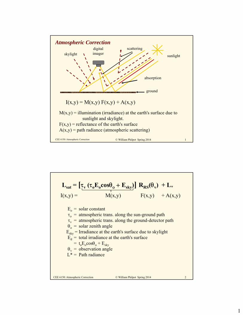
Atmospheric Correction
I(x,y) = M(x,y) F(x,y) + A(x,y)
digitalimager
ground
sunlightskylight
absorption
scattering
M(x,y) = illumination (irradiance) at the earth's surface due to sunlight and skylight.
F(x,y) = reflectance of the earth's surfaceA(x,y) = path radiance (atmospheric scattering)
2© William Philpot Spring 2014CEE 6150: Atmospheric Correction
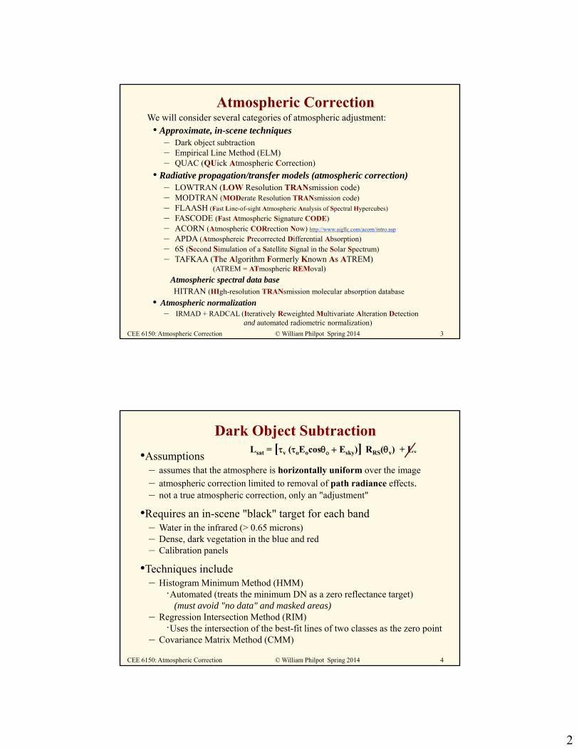
Lsat = [v (oEocos Esky)] RRS(v) + L*
Eo = solar constant = atmospheric trans. along the sun-ground path v = atmospheric trans. along the ground-detector patho = solar zenith angle
Esky = Irradiance at the earth's surface due to skylightEd = total irradiance at the earth's surface
= toEocoso + Esky
v = observation angleL* = Path radiance
I(x,y) = M(x,y) F(x,y) + A(x,y)
2
3© William Philpot Spring 2014CEE 6150: Atmospheric Correction
Atmospheric CorrectionWe will consider several categories of atmospheric adjustment:• Approximate, in-scene techniques
– Dark object subtraction– Empirical Line Method (ELM)– QUAC (QUick Atmospheric Correction)
• Radiative propagation/transfer models (atmospheric correction)– LOWTRAN (LOW Resolution TRANsmission code)– MODTRAN (MODerate Resolution TRANsmission code)– FLAASH (Fast Line-of-sight Atmospheric Analysis of Spectral Hypercubes)
– FASCODE (Fast Atmospheric Signature CODE)– ACORN (Atmospheric CORrection Now) http://www.aigllc.com/acorn/intro.asp
– APDA (Atmosphereic Precorrected Differential Absorption)– 6S (Second Simulation of a Satellite Signal in the Solar Spectrum)– TAFKAA (The Algorithm Formerly Known As ATREM)
(ATREM = ATmospheric REMoval)
Atmospheric spectral data baseHITRAN (HIgh-resolution TRANsmission molecular absorption database
• Atmospheric normalization– IRMAD + RADCAL (Iteratively Reweighted Multivariate Alteration Detection
and automated radiometric normalization)
4© William Philpot Spring 2014CEE 6150: Atmospheric Correction
Dark Object Subtraction
•Assumptions– assumes that the atmosphere is horizontally uniform over the image
– atmospheric correction limited to removal of path radiance effects.– not a true atmospheric correction, only an "adjustment"
•Requires an in-scene "black" target for each band– Water in the infrared (> 0.65 microns)– Dense, dark vegetation in the blue and red– Calibration panels
•Techniques include– Histogram Minimum Method (HMM)
·Automated (treats the minimum DN as a zero reflectance target)(must avoid "no data" and masked areas)
– Regression Intersection Method (RIM)·Uses the intersection of the best-fit lines of two classes as the zero point
– Covariance Matrix Method (CMM)
Lsat = [v (oEocos Esky)] RRS(v) + L*

3
5© William Philpot Spring 2014CEE 6150: Atmospheric Correction
Dark object subtraction
• If the atmosphere is uniform over the scene, and
• If a black (zero reflectance) object exists @ each wavelength then where:
Rmin( ) = 0; ∗
==> correct for path radiance by subtracting the gray value of the dark object pixel from the gray value of every other pixel in the image:
Problems:
• does not account for spatial variation in the atmosphere (full-scene correction).
• truly "dark" values are rare.
Lsat = [v (oEocosEsky)] RRS(v) + L*
assumed to be spatially constant
Lsat , , Rmin( ) = [v (oEocosEsky)] RRS(v) + L*
6© William Philpot Spring 2014CEE 6150: Atmospheric Correction
Empircal Line Method (ELM)
Empirical Line calibration method (ELM) Roberts D. A., Smith M. O., and Adams J. B. (1993), Green vegetation, non-photosynthetic
vegetation and soils in AVIRIS data, Remote Sens. Environ. 44: 255-269.
• Assumptions– assumes a constant atmosphere over the image – know targets (Lambertian)
• Requires 2 known ground truths to perform the regression.– In-scene targets– Calibration panels
Rin situ
Lsa
t
L*
- Radiance, L, (or DN) is taken from the image.- R may be based on
• in-field measurements, • laboratory measurements or • predicted by model

4
7© William Philpot Spring 2014CEE 6150: Atmospheric Correction
ELM with in-scene targets
Significant potential for error if only limited samples are available
or if target variability is high.
Better results are likely if multiple sample pairs are used
and the brightness range is large.
Band 1Band 1
R()
DNorL
soilin-scenesample
in-scenesample
deep vegetation
R()
soil
deep vegetation
8© William Philpot Spring 2014CEE 6150: Atmospheric Correction
ELM pros & cons
Pros
• removes atmospheric and sensor artifacts
• simple and direct if good ground data available
• results are in terms of reflectance
Cons
• requires large known targets
• assumes uniform correction across image
• can introduce sizeable errors if the reference reflectance is
not well-known.
5
9© William Philpot Spring 2014CEE 6150: Atmospheric Correction
QUAC: Quick Atmospheric CorrectionQUAC is based on the empirical finding that the average reflectance of diverse material spectra is not dependent the specific scene provided that:
• There are at least 10 diverse materials in a scene.• The spectral standard deviation of reflectance for a collection of diverse
materials is a nearly wavelength-independent constant, and • There are sufficiently dark pixels in a scene to allow for a good estimation of
the baseline spectrum.
Pros• processing is much faster compared to first-principles methods. • allows for any view angle or solar elevation angle. • relatively insensitive to radiometric or wavelength calibration• aerosol optical depth retrieval does not require the presence of dark pixels.
Cons• a more approximate atmospheric correction than FLAASH® or other
physics-based first-principles methods• generally producing reflectance spectra within +/-15% of the other methods.
10© William Philpot Spring 2014CEE 6150: Atmospheric Correction
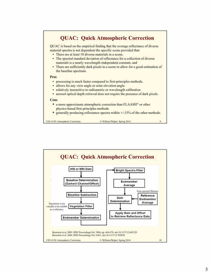
QUAC: Quick Atmospheric Correction
Bernstein et al, 2005. SPIE Proceedings,Vol. 5806, pp. 668-678. doi:10.1117/12.603359Bernstein et al. 2006. SPIE Proceedings,Vol. 6362., doi:10.1117/12.705038
Vegetation is too variable to be reliable
as a reference.
from spectral libraries

6
11© William Philpot Spring 2014CEE 6150: Atmospheric Correction
Lsat = [v (oEocos Esky)] RRS(v) + L*
Eo = solar constant = atmospheric trans. along the sun-ground path o = atmospheric trans. along the ground-detector patho = solar zenith angle
Esky = Irradiance at the earth's surface due to skylightEd = total irradiance at the earth's surface
= toEocoso + Esky
v = observation angleL* = Path radiance
Need to be confident of the radiance [Wmst-1]
good calibration of the sensor
12© William Philpot Spring 2014CEE 6150: Atmospheric Correction
Atmospheric Correction Using Models and Spectral Data
1) Calibration of the detection system– noise mitigation
• dark current• noise sources (spectral, temporal, spatial)
– spectral calibration• band center• relative spectral response• FWHM
– absolute calibration to radiance
2) Apply atmospheric correction– atmospheric transmission– atmospheric scattering path radiance– atmospheric absorption– compute reflectance at the surface
Laboratory and
in-flight
7
13© William Philpot Spring 2014CEE 6150: Atmospheric Correction
AVIRIS: Radiometric Calibration
Laboratory Radiometric Calibration
– dark level
– noise characterization
– intensity (radiometric) calibration
(using calibration lamps, integrating sphere)
– spectral calibration (using laser lines, narrow-band filters)
• location of the band center
• characterization of the band width
14© William Philpot Spring 2014CEE 6150: Atmospheric Correction
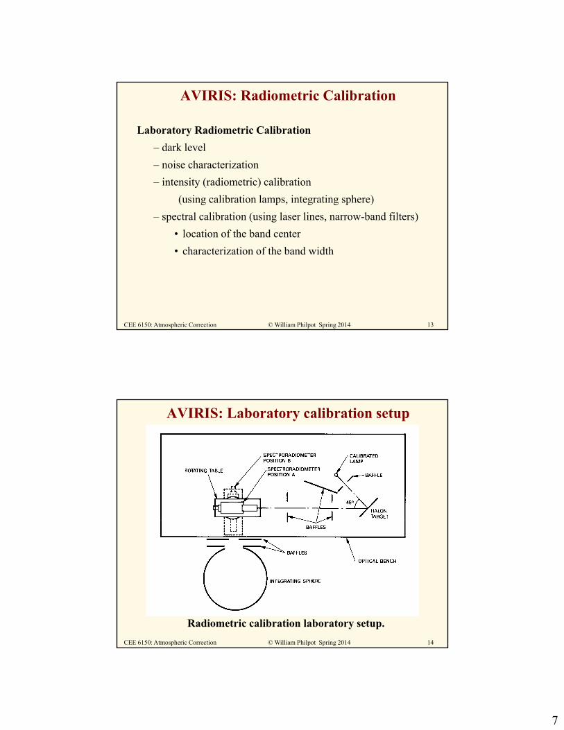
Radiometric calibration laboratory setup.
AVIRIS: Laboratory calibration setup
8
15© William Philpot Spring 2014CEE 6150: Atmospheric Correction
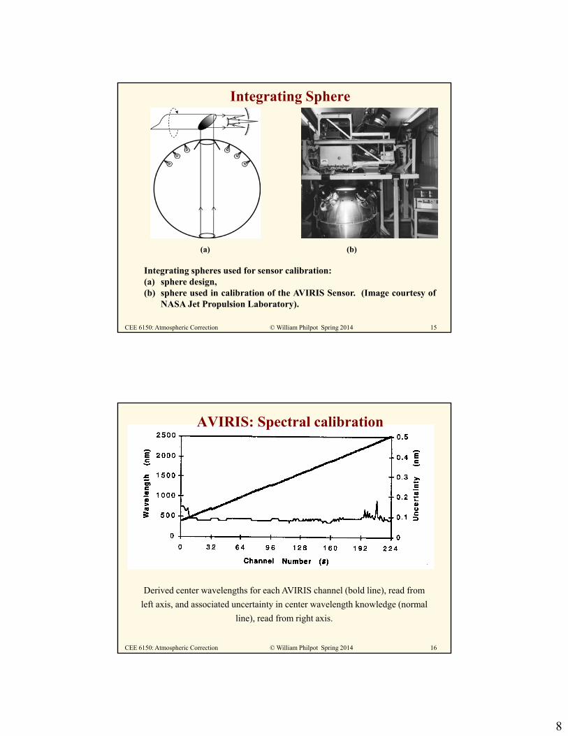
Integrating spheres used for sensor calibration:(a) sphere design,(b) sphere used in calibration of the AVIRIS Sensor. (Image courtesy of
NASA Jet Propulsion Laboratory).
Integrating Sphere
(a) (b)
16© William Philpot Spring 2014CEE 6150: Atmospheric Correction
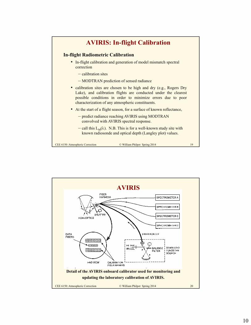
Derived center wavelengths for each AVIRIS channel (bold line), read from
left axis, and associated uncertainty in center wavelength knowledge (normal
line), read from right axis.
AVIRIS: Spectral calibration

9
17© William Philpot Spring 2014CEE 6150: Atmospheric Correction
Typical spectral response function for a single AVIRIS channel with error
bars and best fit Gaussian curve from which center wavelength, FWHM
bandwidth and uncertainties are derived.
AVIRIS: Spectral calibration
18© William Philpot Spring 2014CEE 6150: Atmospheric Correction
AVIRIS: S/N ratio
Green, R.O. et al. (1998) Imaging Spectroscopy and the Airborne Visible/Infrared Imaging Spectrometer (AVIRIS). Remote Sensing of Environment, 65:227-248. doi: 10.1016/S0034-4257(98)00064-9
10
19© William Philpot Spring 2014CEE 6150: Atmospheric Correction
AVIRIS: In-flight Calibration
In-flight Radiometric Calibration
• In-flight calibration and generation of model mismatch spectral correction
– calibration sites
– MODTRAN prediction of sensed radiance
• calibration sites are chosen to be high and dry (e.g., Rogers DryLake), and calibration flights are conducted under the clearestpossible conditions in order to minimize errors due to poorcharacterization of any atmospheric constituents.
• At the start of a flight season, for a surface of known reflectance,
– predict radiance reaching AVIRIS using MODTRAN convolved with AVIRIS spectral response.
– call this LM(). N.B. This is for a well-known study site with known radiosonde and optical depth (Langley plot) values.
20© William Philpot Spring 2014CEE 6150: Atmospheric Correction
Detail of the AVIRIS onboard calibrator used for monitoring and
updating the laboratory calibration of AVIRIS.
AVIRIS

11
21© William Philpot Spring 2014CEE 6150: Atmospheric Correction
HITRAN
• Acronym for HIgh-resolution TRANsmission molecular absorption database
• HITRAN is a compilation of spectral line parameters for 36 different molecules – started by the Air Force Cambridge Research Laboratories (AFCRL) in
the late 1960's– Parameters include: line position, strength, half-width, lower energy
level, etc.
• used by a variety of computer codes (e.g., LOWTRAN, MODTRAN, FASCODE) to predict and simulate the transmission and emission of light in the atmosphere.
• See http://www.hitran.com/
22© William Philpot Spring 2014CEE 6150: Atmospheric Correction
Thermosphere
Mesopause
Mesopause
MesosphereStratopause
StratosphereTropopause
Troposphere
Temperature-100 –60 0 20 200 1,750
-148 –76 32 68 392 3,182
°C
°F
120
85
6050
15
0
74
63
3731
9
0
km
600
mi
372
Altitude
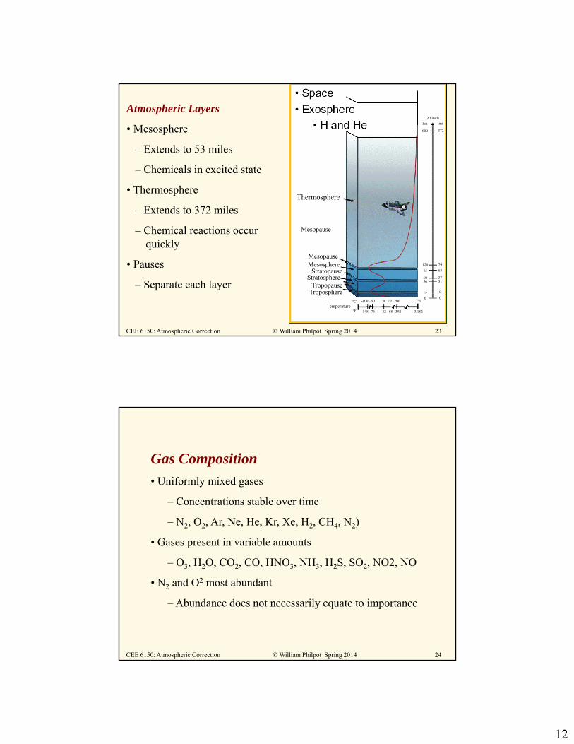
Atmospheric Layers
• Troposphere
– Surface to 5-9 miles
– Most dense
– Almost all weather
• Stratosphere
– Extends to 31 miles
– Includes ozone layer
• Absorbs UV
– 99 % air below top of this layer
12
23© William Philpot Spring 2014CEE 6150: Atmospheric Correction
Thermosphere
Mesopause
Mesopause
MesosphereStratopause
StratosphereTropopause
Troposphere
Temperature-100 –60 0 20 200 1,750
-148 –76 32 68 392 3,182
°C
°F
120
85
6050
15
0
74
63
3731
9
0
km
600
mi
372
Altitude
Atmospheric Layers
• Mesosphere
– Extends to 53 miles
– Chemicals in excited state
• Thermosphere
– Extends to 372 miles
– Chemical reactions occur quickly
• Pauses
– Separate each layer
24© William Philpot Spring 2014CEE 6150: Atmospheric Correction
Gas Composition
• Uniformly mixed gases
– Concentrations stable over time
– N2, O2, Ar, Ne, He, Kr, Xe, H2, CH4, N2)
• Gases present in variable amounts
– O3, H2O, CO2, CO, HNO3, NH3, H2S, SO2, NO2, NO
• N2 and O2 most abundant
– Abundance does not necessarily equate to importance

13
25© William Philpot Spring 2014CEE 6150: Atmospheric Correction
Particle Composition• Particle Composition
• Vary in size and shape
• Size-distribution functions– Concentration as a function of particle radius
• Height-distribution functions– Concentration as a function of altitude
• Two classes of particles– Aerosol (radius < 1μm)
• Suspended in the atmosphere (Most near surface of earth)• Increases scattering over molecular scattering
– Hydrometers (radius > 1μm)• Water-dominated particles• Shorter lifespan
26© William Philpot Spring 2014CEE 6150: Atmospheric Correction
Aerosols• Dust
– Terrestrial• Volcanoes (Stratosphere)• Soil-based dusts• Industry and construction
– Extraterrestrial (predominate in outer atmosphere)• Planetary accretion• Meteoroids
• Hygroscopic (depend on relative humidity)– Vegetation
• Give off hydrocarbons which oxidize or nucleate into complex tars and resins
– Sea• Sea salt (injected by bursting bubbles)• Concentration highly dependent on local wind velocity
– Combustion by-products• Undergo photochemical reactions to produce hygroscopic particles

14
27© William Philpot Spring 2014CEE 6150: Atmospheric Correction
LOWTRANLOWTRAN: LOW resolution TRANsmission code• Single-parameter (pressure) band model
• Computes transmittance averaged over a spectral band
• 20 cm-1 resolution from 0-50,000 cm-1 (~2nm in the VNIR)
• Does not fully represent the correct temperature dependence
• Three classes of atmospheric gases– water vapor– ozone– uniformly mixed gases
• Atmosphere divided into 32 layers. – 0-100,000 km altitude
– Layer thickness varies from 1 km to 30 km
– Characteristics of each layer determined by inputs and standard models of various regions and seasons
28© William Philpot Spring 2014CEE 6150: Atmospheric Correction
MODTRANMODTRAN: MODerate resolution TRANsmission codeSame as LOWTRAN except:
• Two-parameter (pressure, temperature) band model
• Computes transmittance averaged over a spectral band
• Calculates atmospheric transmittance and radiance resolution from 0-50,000 cm-1 at 2 cm-1 resolution
• More realistic temperature-dependent model
• Includes high-altitude transmittance/radiance calculation up to 60 km.
• Includes water vapor, carbon dioxide, ozone, nitrous oxide, carbon monoxide, methane, oxygen, nitric oxide, sulfur dioxide, ammonia, and nitric acid.
http://www.modtran.org/features/index.htmlATCOR http://www.rese.ch/atcor/

15
29© William Philpot Spring 2014CEE 6150: Atmospheric Correction
FASCODE
FASCODE: Fast Atmospheric Signature Code• High spectral-resolution code
• Uses the HITRAN database directly
• Required for modeling very narrow optical bandwidth radiation (e.g., laser)
• Characterization of the aerosol and molecular medium is similar to LOWTRAN
30© William Philpot Spring 2014CEE 6150: Atmospheric Correction
6S Second Simulation of the Satellite Signal in the Solar Spectrum
Improved version of 5S developed by Didier Tanre at the Laboratoire d'Optique Atmospherique
Inputs to the 6S model:
• Viewing and Illumination geometry: solar azimuth, view angle etc.
• Atmospheric model - there are 5 standard models supplied with the code, which can be used depending on the time of year and latitude - Tropical, Mid-latitude (summer), Mid-latitude (winter), Subarctic (summer), Subarctic (winter).
• Aerosol model - this has 4 components - dust, oceanic, water-soluble and soot. Again, the 5S model has standard models, namely continental, maritime and urban.
• Aerosol concentration - in terms of either the visibility in km, or the aerosol optical depth at 550 nm. (Usually set by iterative approximations.)
• Spectral band under consideration.
6S: http://6s.ltdri.org//
16
31© William Philpot Spring 2014CEE 6150: Atmospheric Correction
Critical Atmospheric Parameters
• density of the atmosphere (pressure depth)
• aerosols type and number
• water – column water vapor
32© William Philpot Spring 2014CEE 6150: Atmospheric Correction
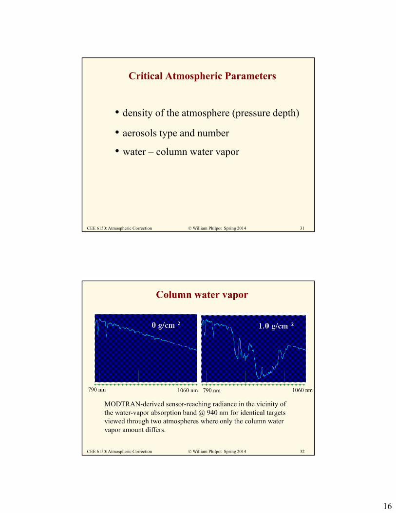
Column water vapor
MODTRAN-derived sensor-reaching radiance in the vicinity of the water-vapor absorption band @ 940 nm for identical targets viewed through two atmospheres where only the column water vapor amount differs.
790 nm 1060 nm 790 nm 1060 nm
17
33© William Philpot Spring 2014CEE 6150: Atmospheric Correction
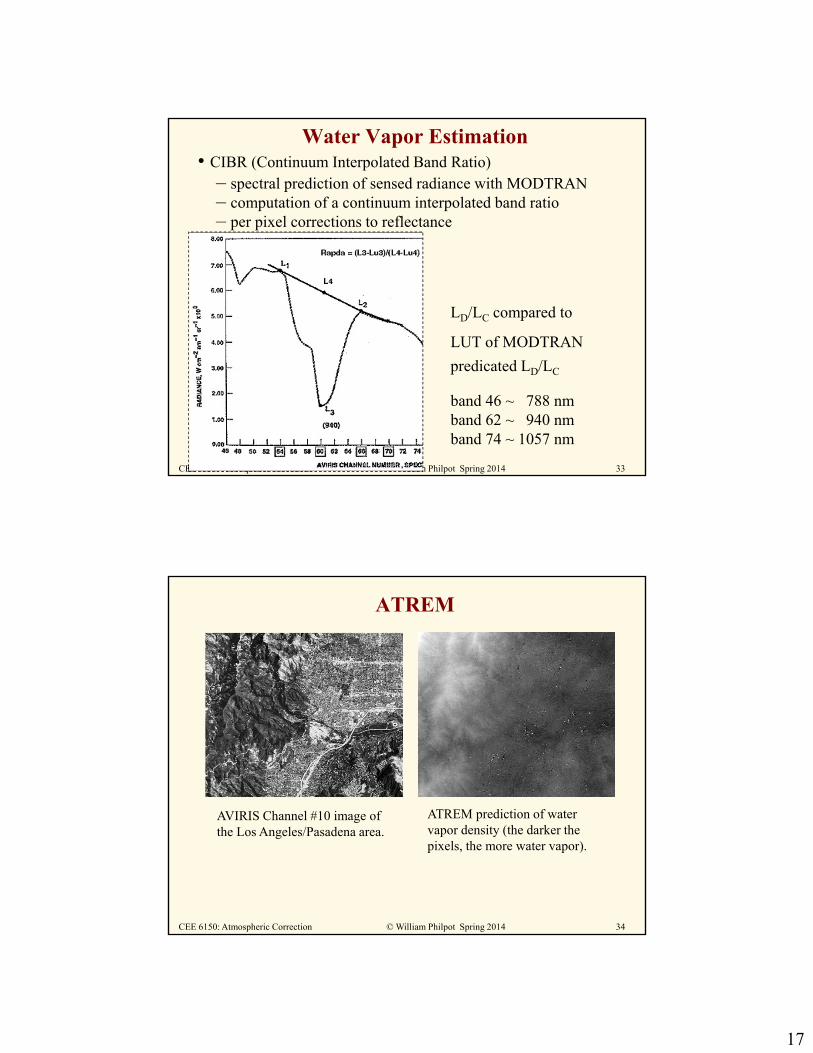
Water Vapor Estimation• CIBR (Continuum Interpolated Band Ratio)
– spectral prediction of sensed radiance with MODTRAN– computation of a continuum interpolated band ratio– per pixel corrections to reflectance
LD/LC compared to
LUT of MODTRAN
predicated LD/LC
band 46 ~ 788 nmband 62 ~ 940 nmband 74 ~ 1057 nm
34© William Philpot Spring 2014CEE 6150: Atmospheric Correction
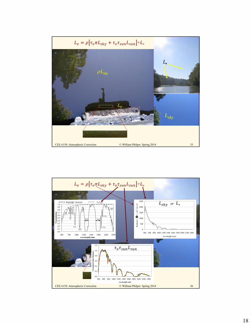
ATREM
AVIRIS Channel #10 image of the Los Angeles/Pasadena area.
ATREM prediction of water vapor density (the darker the pixels, the more water vapor).
18
35© William Philpot Spring 2014CEE 6150: Atmospheric Correction
skyL
L
skyL
+ ∗
36© William Philpot Spring 2014CEE 6150: Atmospheric Correction
+ ∗
H20
H20
H20 H20
H20
CO2
CO2
O2
O2
O3H2O H2O
0.00.10.20.30.40.50.60.70.80.91.0
400 700 1000 1300 1600 1900 2200 2500wavelength (nm)
Tra
nsm
issi
on
Rayleigh+Aerosol vsun
0.0
0.2
0.4
0.6
0.8
1.0
1.2
400 600 800 1000 1200 1400 1600 1800 2000 2200 2400
wavelength (nm)
Nor
mal
ized
Sol
ar R
adia
nce
0
500
1000
1500
2000
2500
400 600 800 1000 1200 1400 1600 1800 2000 2200 2400
wavelength (nm)
Rad
ianc
e (
W /
cm
2 nm
sr) or ∗

19
37© William Philpot Spring 2014CEE 6150: Atmospheric Correction
38© William Philpot Spring 2014CEE 6150: Atmospheric Correction
ATMOSPHERIC CORRECTION
GOAL: To develop a process that will
1. be less dependent (ideally, independent) on field measurements at the time of the data collect
2. correct for the atmosphere on a pixel-by-pixel basis,
3. not require excessive computation time,
4. be radiometrically correct, and
5. be more rigorous in its treatment of atmospheric parameters than previous methodologies.

20
39© William Philpot Spring 2014CEE 6150: Atmospheric Correction
Atmospheric Correction
Competitors:1. ATREM (Goetz and Gao, 1993) (now TAFKAA)
ATmosphere REMoval Programhttp://cires.colorado.edu/cses/atrem.html#atrem_ref
2. the NLLSSF method developed (Robert Green, 1989)(Non-Linear Least Square Spectral Fit)
3. the APDA method (Borel and Schläpfer, 1996)Atmospheric Pre-corrected Differential Absorptionhttp://popo.jpl.nasa.gov/docs/workshops/96_docs/3.PDF
These algorithms all predict column water vapor from spectral water absorption features in hyperspectral image data.
40© William Philpot Spring 2014CEE 6150: Atmospheric Correction
ATREM
1. Atmospheric transmission is calculated using the Malkmus narrow band model and a pressure scaling approximation
This is done for seven gases (water vapor, ozone, oxygen, carbon monoxide, carbon dioxide, methane, and nitrous oxide).
2. Atmospheric scattering is modeled using the 6S code.
3. Since water vapor has high spatial and temporal variations, this gas is removed on a pixel by pixel basis. The amount of water vapor for each pixel is derived from AVIRIS data using the 0.94-and the 1.14- µm water vapor bands and a three channeling ratio technique. The derived water vapor values are then used for modeling water vapor absorption effects in the entire 0.4-2.5 µm region.

21
41© William Philpot Spring 2014CEE 6150: Atmospheric Correction
TAFKAA (the Algorithm Formerly Known As ATREM)
B.-C. Gao, M. J. Montes, Z. Ahmad, and C. O. Davis, “Atmospheric correction algorithm for hyperspectral remote sensing of ocean color from space,” Appl. Opt. 39, 887-896 (2000).
M. J. Montes, B.-C. Gao, and C. O. Davis, “A new algorithm for atmospheric correction of hypespectral remote sensing data,” in Geo-Spatial Image and Data Exploitation II, W. E. Roper, ed., Proc. SPIE 4383, 23-30 (2001).
42© William Philpot Spring 2014CEE 6150: Atmospheric Correction
Atmospheric CalibrationIn general:
scattering dominates below 1 μm; absorption dominates above 1 μm.
Top of atmosphere reflectance
Tanré 1960 claims
cos
sE
Lp
ssussd
ag
1
)(
Rearranging yields:
1
a
gsdsua
g
s
s = single scattering albedo =total scattering
total scattering + total absorption

22
43© William Philpot Spring 2014CEE 6150: Atmospheric Correction
Atmospheric Calibration
where A - F are expressed in apparent reflectance (TOA) averaged over a predefined set of AVIRIS bands designed to characterize the absorption feature and its wings.
0.85 1.20wavelength
Ap
par
ent
refl
ecta
nce
A
B
C D
E
F
0
2
g 0.94
g 1.14
B( 0.94) 2
A C
E( 1.14) 2
D E
An apparent reflectance spectrum with relevant positions and widths of spectral regions used in three channel rationing being illustrated.
44© William Philpot Spring 2014CEE 6150: Atmospheric Correction
Water Vapor EstimationComparing the average of the mean effective transmission in the two absorption regions with theoretical values predicted using radiation propagation models, you can use LUT to obtain an estimate of water vapor concentration on a pixel-by-pixel basis.
Step 1. from lat, long, time of day (T.O.D.) and day of the year (D.O.Y.)
Step 2. g calculated based on models and atm path. For H2O, several spectra computed as function of total column H2O range 0 - 10 cm. So we end up with many g spectra. The band ratio transmittances can be calculated for each spectra.
Step 3. a, s, us and ud are calculated using 6S which assumes no absorption for these calculations.
Step 4. AVIRIS radiance converted to apparent reflectance spectrum (TOA reflectance).
Step 5. Calculate channel ratios at 0.94 and 1.14 µm regions using Equation 3 on the results of Step 4. Compare Step 5 to results of Step 2 and estimate column H2O and corresponding g.
Step 6. g from 5 and inputs from 3 and 4 are used with Equation 2 to estimate reflectance spectra.
23
45© William Philpot Spring 2014CEE 6150: Atmospheric Correction
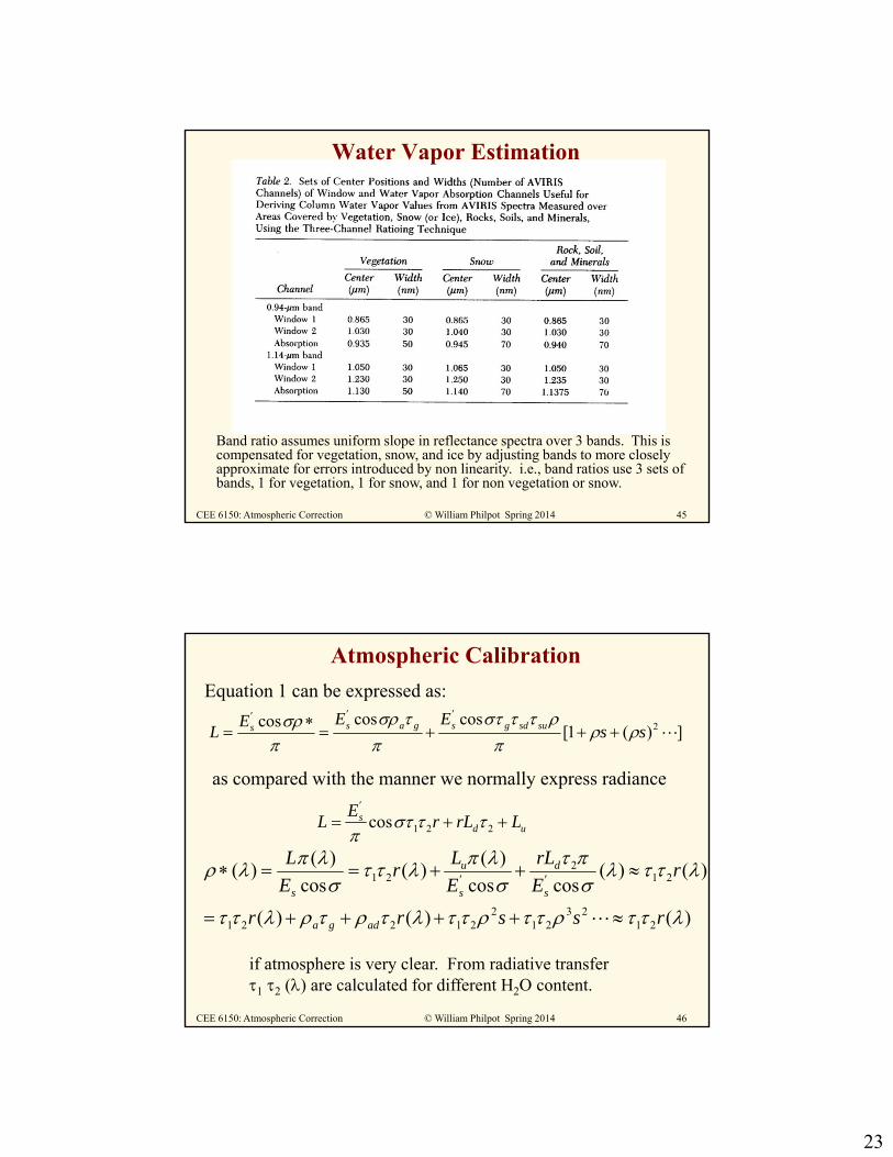
Water Vapor Estimation
Band ratio assumes uniform slope in reflectance spectra over 3 bands. This is compensated for vegetation, snow, and ice by adjusting bands to more closely approximate for errors introduced by non linearity. i.e., band ratios use 3 sets of bands, 1 for vegetation, 1 for snow, and 1 for non vegetation or snow.
46© William Philpot Spring 2014CEE 6150: Atmospheric Correction
Equation 1 can be expressed as:
Atmospheric Calibration
as compared with the manner we normally express radiance
if atmosphere is very clear. From radiative transfer 1 2 () are calculated for different H2O content.
])(1[coscoscos 2ss
EEEL susdgsgass
uds LrLr
EL
221cos
)()()(
)()(coscos
)()(
cos
)()(
2123
212
21221
212
21
rssrr
rE
rL
E
Lr
E
L
adga
s
d
s
u
s
24
47© William Philpot Spring 2014CEE 6150: Atmospheric Correction
Atmospheric Calibration
1 1 2 1
2 3 1 2 2 1 2 3
1 2 1
1 2 2 1 2 3 2 3
From AVIRIS
( r)
( r) ( r)
2 2
From RT Model
( ) r
( ) ( ) r rif 1
2 2
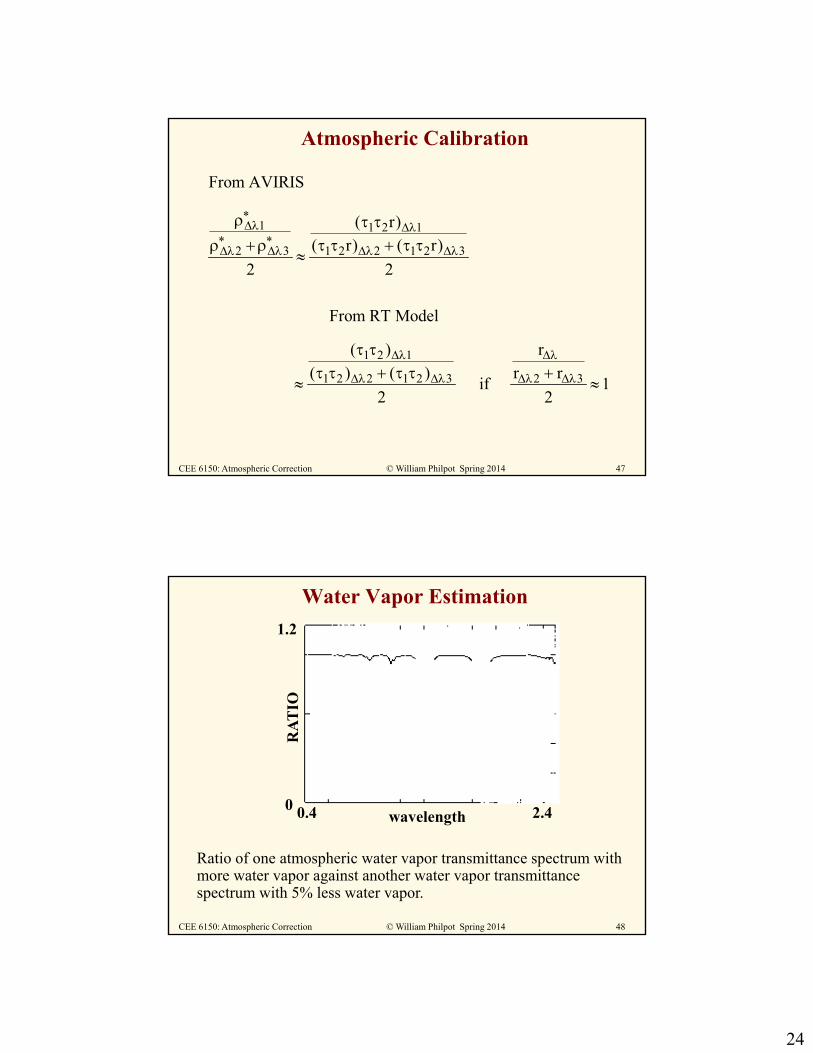
48© William Philpot Spring 2014CEE 6150: Atmospheric Correction
Ratio of one atmospheric water vapor transmittance spectrum with more water vapor against another water vapor transmittance spectrum with 5% less water vapor.
Water Vapor Estimation
wavelength0.4 2.4
RA
TIO
0
1.2

25
49© William Philpot Spring 2014CEE 6150: Atmospheric Correction
• APDA correction to 940 nm ratio
for upwelled radiance using a
column water dependent
upwelled radiance
Water Vapor Estimation with APDA(Atmospheric Pre-corrected Differential Absorption)
• Borel, C.C., and Schlapfer, D. (1996) Atmospheric Pre-Corrected Differential
Absorption Gtechniques to retrieve columnar water vapor: theory and simulations.
In: 6th Annual JPL Airborne Earth Science Workshop, Pasadena (CA), pp. 13-21.
50© William Philpot Spring 2014CEE 6150: Atmospheric Correction
The single channel/band Rapda:
The APDA Technique
which can be extended to more channels:
Relate R ratio with the corresponding water vapor amount (PW)
m atm,m
APDAr1 r1 atm,r1 r2 r2 atm,r2
L L (PW)R
L L L L
m
m atm,mAPDA
r j m atm,m j [ ]
L LR
LIR [ ] ,[L L ]
Solving for water vapor:
( (PW) )wv APDA(PW) R e
1
APDAAPDA
ln RPW(R )
APDALn(R ) (PW)
1Ln(R)
(PW)
26
51© William Philpot Spring 2014CEE 6150: Atmospheric Correction
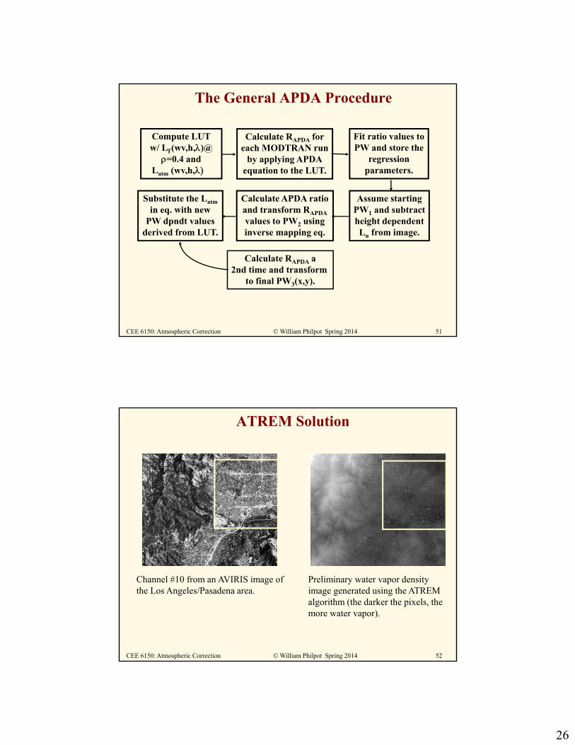
The General APDA Procedure
Compute LUTw/ LT(wv,h,)@
=0.4 and Latm (wv,h,�
Calculate RAPDA foreach MODTRAN run
by applying APDAequation to the LUT.
Fit ratio values toPW and store the
regressionparameters.
Assume startingPW1 and subtractheight dependentLu from image.
Calculate APDA ratioand transform RAPDA
values to PW2 usinginverse mapping eq.
Substitute the Latm
in eq. with newPW dpndt values
derived from LUT.
Calculate RAPDA a2nd time and transform
to final PW3(x,y).
52© William Philpot Spring 2014CEE 6150: Atmospheric Correction
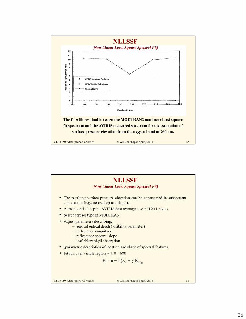
ATREM Solution
Channel #10 from an AVIRIS image of the Los Angeles/Pasadena area.
Preliminary water vapor density image generated using the ATREM algorithm (the darker the pixels, the more water vapor).

27
53© William Philpot Spring 2014CEE 6150: Atmospheric Correction
APDA Solutions
Channel #25 from the cropped AVIRIS image of the Los Angeles/Pasadena area.
Preliminary water vapor density image generated using the APDA algorithm (the darker the pixels, the more water vapor).
54© William Philpot Spring 2014CEE 6150: Atmospheric Correction
NLLSSF (Non-Linear Least Square Spectral Fit)
1) Oxygen - pressure elevation
To estimate the effective height (surface pressure elevation) thestrength of the oxygen absorption band (760 nm) in the AVIRISspectrum is fit to MODTRAN data.
a. To increase sensitivity, average (e.g., 5x5 pixels) to generateAVIRIS spectrum.
b. Iteratively predict oxygen spectra in AVIRIS radiance unitsusing pressure elevation. Use non linear least squares tocontrol the iteration process.
c. Parameters adjusted were pressure elevation, reflectancemagnitude (a), and reflectance slope (b):
R = a + b()
28
55© William Philpot Spring 2014CEE 6150: Atmospheric Correction
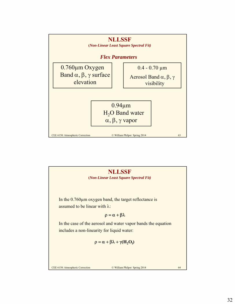
NLLSSF (Non-Linear Least Square Spectral Fit)
The fit with residual between the MODTRAN2 nonlinear least square
fit spectrum and the AVIRIS measured spectrum for the estimation of
surface pressure elevation from the oxygen band at 760 nm.
56© William Philpot Spring 2014CEE 6150: Atmospheric Correction
NLLSSF (Non-Linear Least Square Spectral Fit)
• The resulting surface pressure elevation can be constrained in subsequentcalculations (e.g., aerosol optical depth).
• Aerosol optical depth - AVIRIS data averaged over 11X11 pixels
• Select aerosol type in MODTRAN
• Adjust parameters describing:– aerosol optical depth (visibility parameter)– reflectance magnitude– reflectance spectral slope– leaf chlorophyll absorption
• (parametric description of location and shape of spectral features)
• Fit run over visible region 410 – 680
R = a + b() + Rveg

29
57© William Philpot Spring 2014CEE 6150: Atmospheric Correction
NLLSSF (Non-Linear Least Square Spectral Fit)
Spectral fit for aerosols at the Rose Bowl parking lot.
58© William Philpot Spring 2014CEE 6150: Atmospheric Correction
NLLSSF (Non-Linear Least Square Spectral Fit)
The nonlinear least squares between the AVIRIS measured radiance and the
MODTRAN2 modeled radiance for estimation of aerosol optical depth. The
modeled reflectance required for this fit in the 400 to 600 nm spectral region
is also shown as is the resulting AVIRIS calculated reflectance.

30
59© William Philpot Spring 2014CEE 6150: Atmospheric Correction
NLLSSF (Non-Linear Least Square Spectral Fit)
• Water vapor is determined for each pixel using the (940 absorption feature)
• Fits parameters for
– column water vapor and
– 3 parameters that describe surface reflectance with leafwater.
R = a + b() + Rveg
60© William Philpot Spring 2014CEE 6150: Atmospheric Correction
NLLSSF (Non-Linear Least Square Spectral Fit)
Surface reflectance with leaf water absorption required to achieve accurate fit
between the measured radiance and modeled radiance (see Figure)

31
61© William Philpot Spring 2014CEE 6150: Atmospheric Correction
NLLSSF (Non-Linear Least Square Spectral Fit)
The water content, aerosol optical depth, and pressure elevation can all be fixed on a pixel- by-pixel basis to develop a radiative transfer equation
solution of the form:
1 2 gsa
g
rE cosL r
1 r S
where: Es is exoatmospheric irradiance, is solar declination angle,ra is the effective reflectance of the atmosphere,rg is the reflectance of the ground1 and 2 are sun-target and target-sensor transmissions,S is the single spherical scattering albedo of atmosphere above the
target (rgS accounts for multiple scattering adjacency effects).
62© William Philpot Spring 2014CEE 6150: Atmospheric Correction
NLLSSF (Non-Linear Least Square Spectral Fit)
Solving for rg yields:
g
o 1 2
o a
1r
E cosS
L E r cos /
We may minimize the difference between the sensor radiance and the MODRAN-derived sensor radiance by changing parameters in the governing radiative transfer equation for least-square error (LSE):
g
sensor u env g o 1 2 d 2g
LSE L L L E cos( ) L1 S
g: Lambertian ground reflectance
32
63© William Philpot Spring 2014CEE 6150: Atmospheric Correction
NLLSSF (Non-Linear Least Square Spectral Fit)
0.760µm Oxygen Band , , surface
elevation
0.94µm H2O Band water , , vapor�
0.4 - 0.70 µm
Aerosol Band , , visibility
Flex Parameters
64© William Philpot Spring 2014CEE 6150: Atmospheric Correction
NLLSSF (Non-Linear Least Square Spectral Fit)
In the 0.760µm oxygen band, the target reflectance is
assumed to be linear with :
In the case of the aerosol and water vapor bands the equation
includes a non-linearity for liquid water:
(H2Ol)

33
65© William Philpot Spring 2014CEE 6150: Atmospheric Correction
NLLSSF General Flow Chart of the Algorithm
Using all Solved Parameters, Invert Governing Radiometric Equation and Calculate Ground Reflectance.
Input ConstantParameters(i.e geometry,particle density,etc)
Solve for TotalColumn Water Vapor Using the .94µm band.
Input Image Pixel:Solve for SurfacePressure Depth in.76µm O2 band.
Solve for AtmosphericVisibility Given an Aerosol Type Using.4-7µm bands
66© William Philpot Spring 2014CEE 6150: Atmospheric Correction
NLLSSF Surface Pressure Elevation
0.015
0.0175
0.02
0.0225
0.025
0.0275
0.03
0.745 0.75 0.755 0.76 0.765 0.77 0.775 0.78 0.785
HYDICE Channel Center Wavelength (micron)
HYDICE Sensor
MODTRAN Calculated

34
67© William Philpot Spring 2014CEE 6150: Atmospheric Correction
NLLSSF Curve Fit – Channel Center Wavelength
0
0.005
0.01
0.015
0.02
0.025
0.84 0.86 0.88 0.9 0.92 0.94 0.96 0.98 1 1.02
HYDICE Channel Center Wavelength (microns)
HYDICE Sensor
MODTRAN Calculated
68© William Philpot Spring 2014CEE 6150: Atmospheric Correction
NLLSSF Water Vapor Estimation
– Pressure depth• 760 feature• spectral model prediction and LUT generation• model match – amoeba algorithm
– aerosol number density/visibility• spectral model prediction and LUT generation• model match
– column water vapor• spectral model prediction and LUT generation• model match
– products• reflection spectra • vegetation moisture map• water vapor map • aerosol # density mapping• pressure depth map

35
69© William Philpot Spring 2014CEE 6150: Atmospheric Correction
RIM to generate spectral upwelled radiance estimate
Per image or per region model match to spectral estimate of upwelled radiance from RIM
Per pixel model over visible region NLLSSF
Per pixel atmospheric coefficients for computing inversion equations
or
APDA per pixel iterative ratio match
or
Pressure depth(elevation)
aerosol numberdensity (visibility)
water vapor
wavelength
Rad
ianc
e
MeasuredModeledResidualslocal met
station visibility
radio-sonde
or
elevationand
pressure
Per pixel model match on 760nm oxygen feature
6
Per pixel model match on 940nm water feature NLLSSF
Radiative TransferModel MODTRAN
70© William Philpot Spring 2014CEE 6150: Atmospheric Correction
Estimated image-wide reflectance error for ground targets of 18% reflectance or less
Estimated Image-Wide Reflectance Error for HYDICE Run cr15m50 from NLLSSF 2nd Pass (average of Old panel reflectances less than 18%)
-0.05
-0.045
-0.04
-0.035
-0.03
-0.025
-0.02
-0.015
-0.01
-0.005
0
0.005
0.01
0.015
0.02
400 500 600 700 800 900 1000 1100 1200 1300 1400 1500 1600 1700 1800
Wavelength (nm)
Avg
Ref
lect
ance
Err
or
36
71© William Philpot Spring 2014CEE 6150: Atmospheric Correction
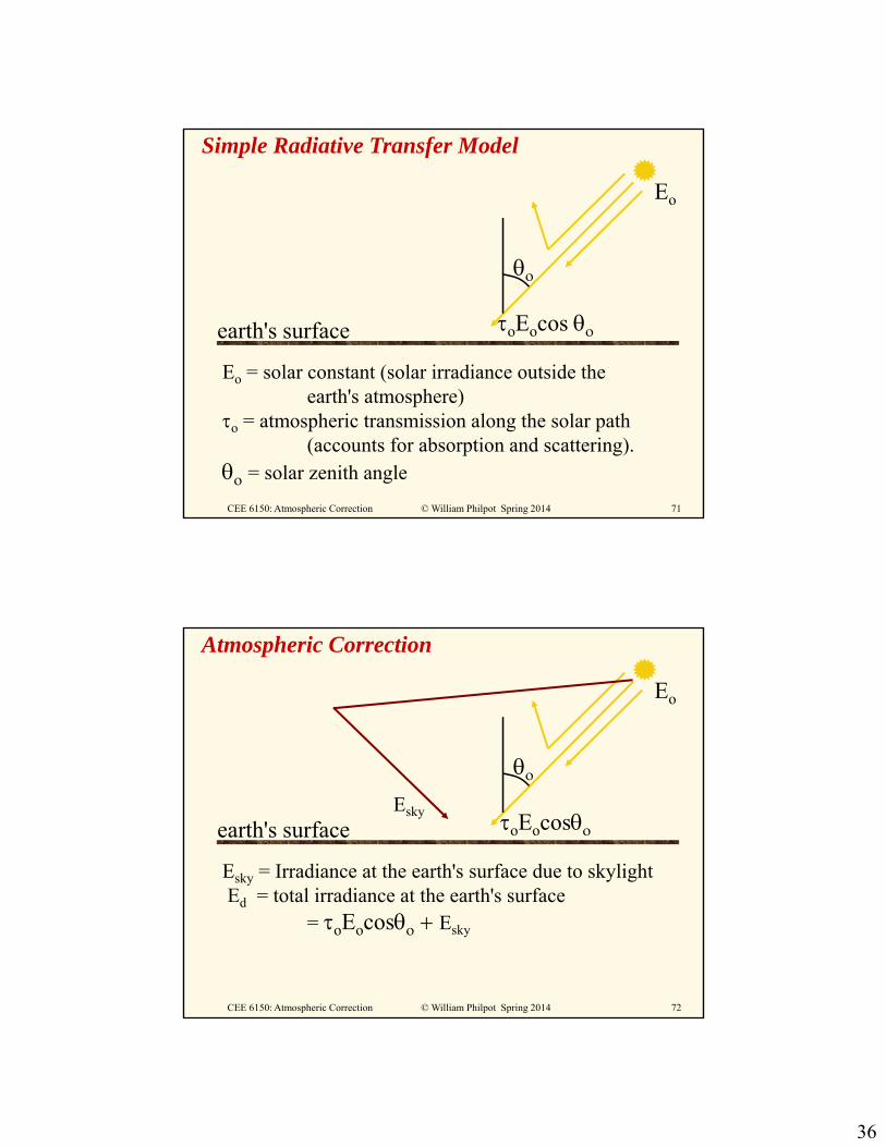
Simple Radiative Transfer Model
Eo = solar constant (solar irradiance outside the earth's atmosphere)
o = atmospheric transmission along the solar path (accounts for absorption and scattering).
= solar zenith angle
Eo
oEocos
earth's surface
72© William Philpot Spring 2014CEE 6150: Atmospheric Correction
Atmospheric Correction
Esky = Irradiance at the earth's surface due to skylightEd = total irradiance at the earth's surface
= oEocos Esky
Eo
oEocos
earth's surfaceEsky
37
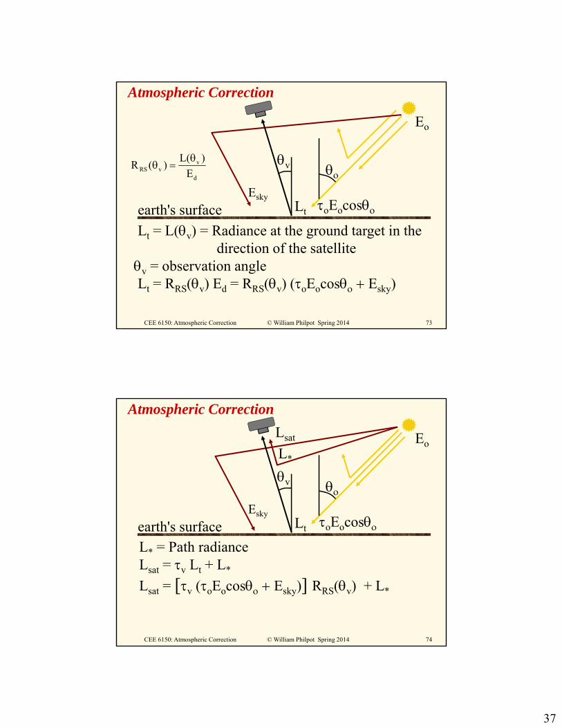
73© William Philpot Spring 2014CEE 6150: Atmospheric Correction
Atmospheric Correction
Eo
oEocos
earth's surfaceEsky
Lt = L(v) = Radiance at the ground target in the direction of the satellite
v = observation angleLt = RRS(v) Ed = RRS(v) (oEocos Esky)
v
Lt
vRS v
d
L( )R ( )
E
74© William Philpot Spring 2014CEE 6150: Atmospheric Correction
Atmospheric Correction
L* = Path radianceLsat = v Lt + L*
Lsat = [v (oEocos Esky)] RRS(v) + L*
Eo
oEocos
earth's surfaceEsky
Lsat
v
Lt
L*

38
75© William Philpot Spring 2014CEE 6150: Atmospheric Correction
2. RatioingSuppose that the illumination and atmosphere are both spatially variable, but differ from band to band only by a constant factor, c, then , , and , ,
(subscripts refer to spectral bands)
then dividing (pixel by pixel) the first band by the second yields a new image:
,,
,=
, , ,
, , ,
If the path radiance is negligible [A1= A2 = 0] or can be removed by another method then
and the new image will be insensitive to variations in illumination and atmosphere.
,,
,=
,
,
76© William Philpot Spring 2014CEE 6150: Atmospheric Correction
Shadow method•Piech and Walker (1971)
– assumes a constant atmosphere over the image – uses the change in radiance received from both the shadowed and
illuminated portions of a several targets.– Requires a broad range of reflectances to be effective– Requires user interaction– Corrects for path radiance and diffuse illumination
Lshade = Ldt2d + L*
Lsun = [Esun/sun + Ldt2]d + L*
Lsun – Lshade = (Esun/sun d
Lshade
Lsun
L*
spectral!
39
77© William Philpot Spring 2014CEE 6150: Atmospheric Correction
78© William Philpot Spring 2014CEE 6150: Atmospheric Correction
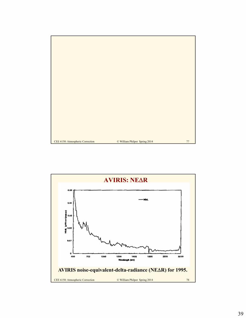
AVIRIS: NER
AVIRIS noise-equivalent-delta-radiance (NER) for 1995.

40
79© William Philpot Spring 2014CEE 6150: Atmospheric Correction
AVIRIS: Radiometric Calibration
where:
is the modeled radiance at the detector
is the observed AVIRIS radiance for the target modeled in generating LM.
vector is the residual miscalibration error between MODTRAN and AVIRIS. In particular, any residual spectral miscalibration will be picked up by this process.
Generate a correction vector
80© William Philpot Spring 2014CEE 6150: Atmospheric Correction
AVIRIS: Calibration ratio
Calibration ratio between AVIRIS and MODTRAN3 derived from theinflight calibration experiment on the 4th of April 1994.

41
81© William Philpot Spring 2014CEE 6150: Atmospheric Correction
AVIRIS: Radiometric Calibration
The onboard calibrator also senses slight changes in detectors
over time. Define a correction vector:
For any spectrum predicted by MODTRAN, the equivalent
AVIRIS spectrum is then given by:
LA() = LM() CM()
1c
2
L ( )C ( )
L ( )
where L1() = lamp radiance at time of in-scene correction
used to generate equation 1 (Day 1), L2() = lamp radiance at
time of flight of current interest (Day 2).
82© William Philpot Spring 2014CEE 6150: Atmospheric Correction
AVIRIS: Radiometric Calibration
Calibration ratio of the on-board calibrator signal for the Pasadena flight to the signal for the in-flight calibration experiment.
To correct AVIRIS radiance on Day 2 to equivalent readings
on Day 1: L1() = L2() Cc()
42
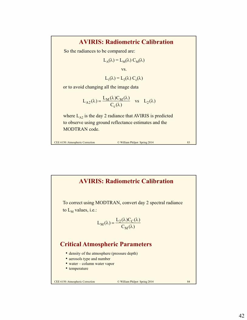
83© William Philpot Spring 2014CEE 6150: Atmospheric Correction
AVIRIS: Radiometric Calibration
or to avoid changing all the image data
So the radiances to be compared are:
LA() = LM() CM()
vs.
L1() = L2() Cc()
M MA2 2
c
L ( )C ( )L ( ) vs L ( )
C ( )
where LA2 is the day 2 radiance that AVIRIS is predicted to observe using ground reflectance estimates and the MODTRAN code.
84© William Philpot Spring 2014CEE 6150: Atmospheric Correction
AVIRIS: Radiometric Calibration
To correct using MODTRAN, convert day 2 spectral radiance
to LM values, i.e.:
2 CM
M
L ( )C ( )L ( )
C ( )
Critical Atmospheric Parameters• density of the atmosphere (pressure depth)• aerosols type and number• water – column water vapor• temperature
43
85© William Philpot Spring 2014CEE 6150: Atmospheric Correction
http://www.vs.afrl.af.mil/ProductLines/IR-Clutter/modtran4.aspx
86© William Philpot Spring 2014CEE 6150: Atmospheric Correction
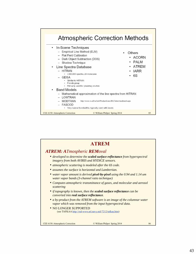
ATREM
ATREM: ATmospheric REMoval• developed to determine the scaled surface reflectance from hyperspectral
imagery from both AVIRIS and HYDICE sensors.
• atmospheric scattering is modeled after the 6S code.
• assumes the surface is horizontal and Lambertian.
• water vapor amount is derived pixel-by-pixel using the 0.94 and 1.14 um water vapor bands (3-channel ratio technique)
• Computes atmospheric transmittance of gases, and molecular and aerosol scattering
• if topography is known, then the scaled surface reflectance can be converted into real surface reflectance.
• a by-product from the ATREM software is an image of the columnar water vapor which was removed from the input hyperspectral data.
• NO LONGER SUPPORTED (see TAFKAA http://rsd-www.nrl.navy.mil/7212/tafkaa.htm)
44
87© William Philpot Spring 2014CEE 6150: Atmospheric Correction
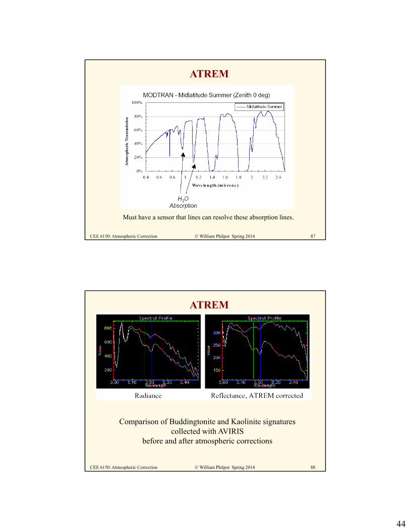
ATREM
Must have a sensor that lines can resolve these absorption lines.
88© William Philpot Spring 2014CEE 6150: Atmospheric Correction
ATREM
Comparison of Buddingtonite and Kaolinite signatures collected with AVIRIS
before and after atmospheric corrections
45
89© William Philpot Spring 2014CEE 6150: Atmospheric Correction
ACORN
ACORN: Atmospheric CORrection Now
• Atmospheric correction between 350 and 2500 nm.
• Uses MODTRAN 4 radiative transfer modeling to calculate the effect of atmospheric gases as well as molecular and aerosol scattering
• Designed to work with multispectral or hyperspectral data
• Operates in several modes ranging from ELM to full MODTRAN modeled atmosphere for hyperspectral data.
Source code: http://www.imspec.com/page4.html
User's Guide: http://www.aigllc.com/pdf/acorn4_ume.pdf
90© William Philpot Spring 2014CEE 6150: Atmospheric Correction
FLAASH
FLAASH: Fast Line-of-Sight Atmospheric Analysis of Spectral Hypercubes
http://www.creaso.com/english/12_swvis/22_flaash/highlit.htm
• Atmospheric correction between 350 and 2500 nm.
• Uses MODTRAN 4 radiative transfer modeling to calculate the effect of atmospheric gases as well as molecular and aerosol scattering
• Operates on a pixel-by-pixel basis, taking advantage of the fact that each pixel in a hyperspectral image contains an independent measurement of the atmospheric water vapor absorption bands (differential absorption).
• Corrects for water vapor, oxygen, carbon dioxide, methane, and ozone in the atmosphere, as well as molecular and aerosol scattering.

46
91© William Philpot Spring 2014CEE 6150: Atmospheric Correction
Pressure Depth
92© William Philpot Spring 2014CEE 6150: Atmospheric Correction
Aerosol Number Density
Retrieved spectra for straight 60% reflector
0.5
0.52
0.54
0.56
0.58
0.6
0.62
0.64
0.66
0.3 0.5 0.7 0.9 1.1
wavelength
Retr
ieve
d S
pectr
a
case 1
case 2
Typical particle size distribution curves for a rural aerosol type.
Visibility Elevation Water vaporCase 1 10.0 0.315 0.05Case 2 70 0.315 0.05