dipartimento di fisica dell’universita’ di milano istituto...
TRANSCRIPT
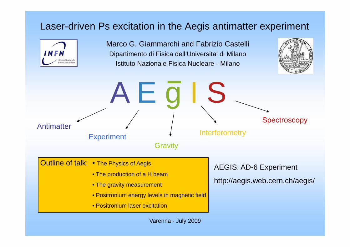
Laser-driven Ps excitation in the Aegis antimatter experiment
Marco G. Giammarchi and Fabrizio CastelliDipartimento di Fisica dell’Universita’ di Milano
Istituto Nazionale Fisica Nucleare - Milano
A E g I SAntimatter
Spectroscopy
Varenna - July 2009
AntimatterExperiment
Gravity
Interferometry
Spectroscopy
Outline of talk: • The Physics of Aegis
• The production of a H beam
• The gravity measurement
• Positronium energy levels in magnetic field
• Positronium laser excitation
AEGIS: AD-6 Experiment
http://aegis.web.cern.ch/aegis/
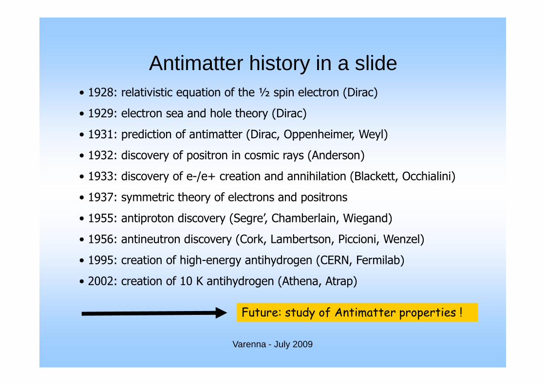
Antimatter history in a slide• 1928: relativistic equation of the ½ spin electron (Dirac)
• 1929: electron sea and hole theory (Dirac)
• 1931: prediction of antimatter (Dirac, Oppenheimer, Weyl)
• 1932: discovery of positron in cosmic rays (Anderson)
• 1933: discovery of e-/e+ creation and annihilation (Blackett, Occhialini)
• 1937: symmetric theory of electrons and positrons
Varenna - July 2009
• 1937: symmetric theory of electrons and positrons
• 1955: antiproton discovery (Segre’, Chamberlain, Wiegand)
• 1956: antineutron discovery (Cork, Lambertson, Piccioni, Wenzel)
• 1995: creation of high-energy antihydrogen (CERN, Fermilab)
• 2002: creation of 10 K antihydrogen (Athena, Atrap)
Future: study of Antimatter properties !

AEGIS Collaboration
LAPP , Annecy, France. P. Nédélec, D. Sillou
CERN, Geneva, Switzerland M. Doser, D. Perini, T. Niinikoski, A. Dudarev, T. W. Eisel, R. Van Weelderen, F. Haug, L.. Dufay-Chanat, J. L.. Servai
Queen’s U Belfast, UK G. Gribakin, H. R. J. Walters
INFN Firenze, Italy G. Ferrari, M. Prevedelli, G. M. Tino
INFN Genova, University of Genova, Italy C. Carraro, V. Lagomarsino, G. Manuzio, G. Testera, S. Zavatarelli
INFN Milano, University of Milano, Italy I. Boscolo, F. Castelli, S. Cialdi, M. G. Giammarchi, D. Trezzi, A. Vairo, F. Villa
INFN Padova/Trento, Univ. Padova, Univ. Trento, Ita ly R. S. Brusa, D. Fabris, M. Lunardon, S. Mariazzi, S. Moretto, G. Nebbia, S. Pesente, G. Viesti
INFN Pavia – Italy University of Brescia, University of Pavia G. Bonomi, A. Fontana, A. Rotondi, A. Zenoni
Varenna - July 2009
INFN Pavia – Italy University of Brescia, University of Pavia G. Bonomi, A. Fontana, A. Rotondi, A. ZenoniMPI- K, Heidelberg, Germany C. Canali, R. Heyne, A. Kellerbauer, C. Morhard, U. Warring
Kirchhoff Institute of Physics U of Heidelberg, Ger many M. K. Oberthaler
INFN Milano, Politecnico di Milano, Italy G. Consolati, A. Dupasquier, R. Ferragut, F. Quasso
INR, Moscow, Russia A. S. Belov, S. N. Gninenko, V. A. Matveev, A. V. Turbabin
ITHEP, Moscow, Russia V. M. Byakov, S. V. Stepanov, D. S. Zvezhinskij
New York University, USA H. H. StrokeLaboratoire Aimé Cotton, Orsay, France L. Cabaret, D. ComparatUniversity of Oslo, Norway O. Rohne, S. Stapnes
CEA Saclay, France M. Chappellier, M. de Combarieu, P. Forget, P. Pari
INRNE, Sofia, Bulgaria N. Djourelov
Czech Technical University, Prague, Czech Republic V. Petráček, D. KrasnickýETH Zurich, Switzerland S. D. Hogan, F. MerktInstitute for Nuclear Problems of the Belarus State University, Belarus G. DrobychevQatar University, Qatar I. Y. Al-Qaradawi

AD (Antiproton Decelerator) at CERN
3 x 10⁷ antiprotons / 100 sec 6 MeV 104 p / 100 sec
Varenna - July 2009
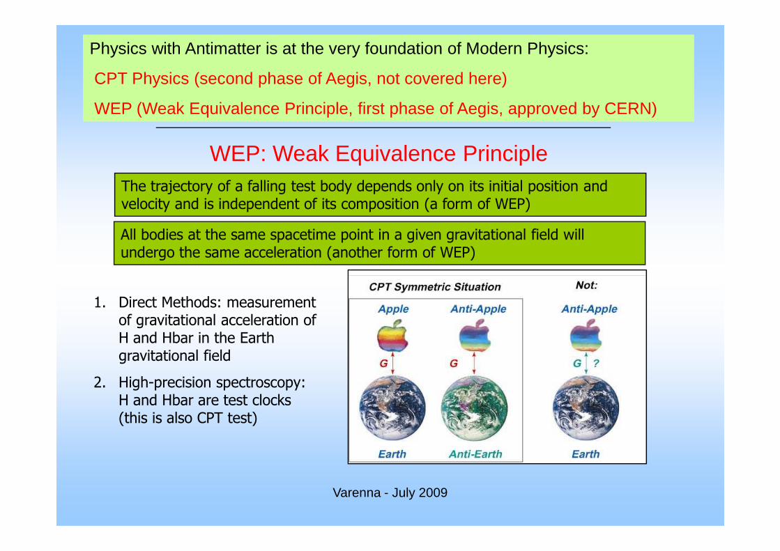
Physics with Antimatter is at the very foundation of Modern Physics:
CPT Physics (second phase of Aegis, not covered here)
WEP (Weak Equivalence Principle, first phase of Aegis, approved by CERN)
WEP: Weak Equivalence PrincipleThe trajectory of a falling test body depends only on its initial position and velocity and is independent of its composition (a form of WEP)
All bodies at the same spacetime point in a given gravitational field will undergo the same acceleration (another form of WEP)
Varenna - July 2009
1. Direct Methods: measurement of gravitational acceleration of H and Hbar in the Earth gravitational field
2. High-precision spectroscopy: H and Hbar are test clocks (this is also CPT test)
10-18
10-16
WEP tests on matter system
10-14
10-12
10-10
10-4
10-6
10-8Matter limit 1310−≤
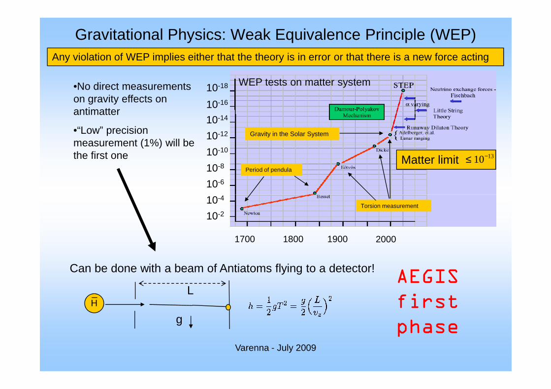
Gravitational Physics: Weak Equivalence Principle (WEP)
•No direct measurements on gravity effects on antimatter
•“Low” precision measurement (1%) will be the first one
Period of pendula
Gravity in the Solar System
Any violation of WEP implies either that the theory is in error or that there is a new force acting
Varenna - July 2009
10-4
10-2
1700 19001800 2000
Can be done with a beam of Antiatoms flying to a detector!AEGIS
first
phaseg
HL
Torsion measurement

Production Methods
e+
p
(A) (B)
p + e+ H + hν
p + e+ + e+ H + e+
I. ANTIPROTON + POSITRON (exp.demonstration: ATHENA and ATRAP)
Varenna - July 2009
p
II. ANTIPROTON + RYDBERG POSITRONIUM (exp.demonstra tion: ATRAP)
p + Ps* H + e-
EXPERIMENTAL RESULTS:• TBR seems to be the dominant process (highly exicited antihydrogen)• Warm antihydrogen atoms (production when vantiproton ~ vpositron)
PROMISING TECHNIQUE:• Control of the antihydrogen quantum state• Cold antihydrogen atoms (vantihydrogen ~ vantiproton) Production
Method in AEGIS
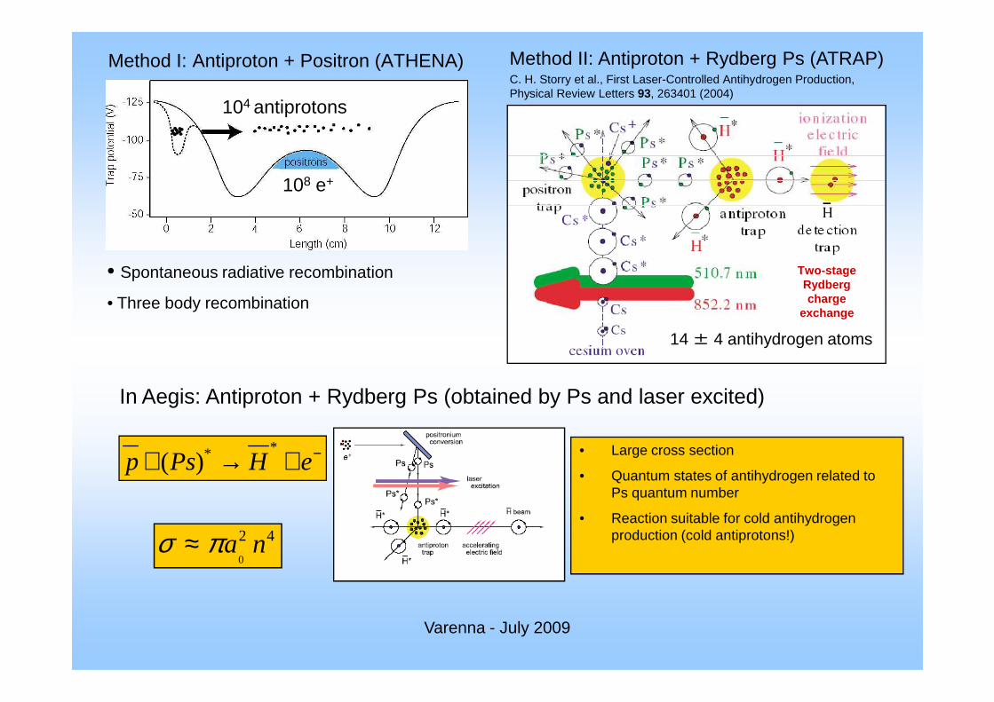
Method I: Antiproton + Positron (ATHENA)
104 antiprotons
108 e+
• Spontaneous radiative recombination
• Three body recombination
14 ± 4 antihydrogen atoms
Method II: Antiproton + Rydberg Ps (ATRAP)
Two-stage Rydberg charge
exchange
C. H. Storry et al., First Laser-Controlled Antihydrogen Production, Physical Review Letters 93, 263401 (2004)
Varenna - July 2009
In Aegis: Antiproton + Rydberg Ps (obtained by Ps and laser excited)
−+→+ eHPsp**)(
0
2 4a nσ π≈
• Large cross section
• Quantum states of antihydrogen related to Ps quantum number
• Reaction suitable for cold antihydrogen production (cold antiprotons!)
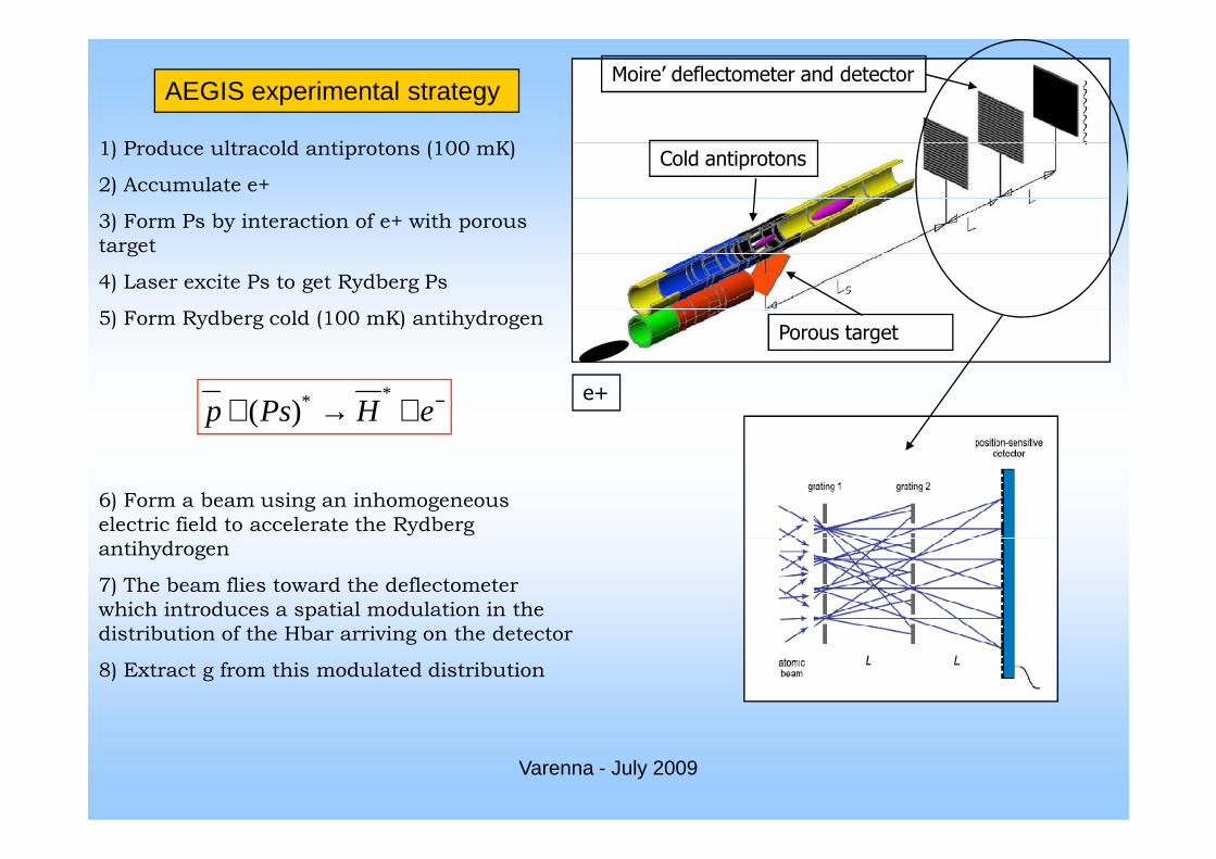
1) Produce ultracold antiprotons (100 mK)
2) Accumulate e+
3) Form Ps by interaction of e+ with porous
target
4) Laser excite Ps to get Rydberg Ps
5) Form Rydberg cold (100 mK) antihydrogen
Cold antiprotons
e+
Porous target
Moire’ deflectometer and detector
−+→+ eHPsp**)(
AEGIS experimental strategy
Varenna - July 2009
6) Form a beam using an inhomogeneous
electric field to accelerate the Rydberg
antihydrogen
7) The beam flies toward the deflectometer
which introduces a spatial modulation in the
distribution of the Hbar arriving on the detector
8) Extract g from this modulated distribution
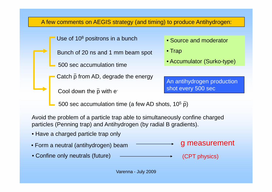
A few comments on AEGIS strategy (and timing) to produce Antihydrogen:
• Source and moderator
• Trap
• Accumulator (Surko-type)
Bunch of 20 ns and 1 mm beam spot
Use of 108 positrons in a bunch
500 sec accumulation time
Catch p from AD, degrade the energy
Cool down the p with e-
An antihydrogen production shot every 500 sec
Varenna - July 2009
Avoid the problem of a particle trap able to simultaneously confine charged particles (Penning trap) and Antihydrogen (by radial B gradients).
• Have a charged particle trap only
• Form a neutral (antihydrogen) beam g measurement
• Confine only neutrals (future) (CPT physics)
500 sec accumulation time (a few AD shots, 105 p)
Ps
Vacuum Solid
Positron beam
Ps
Ps
e+
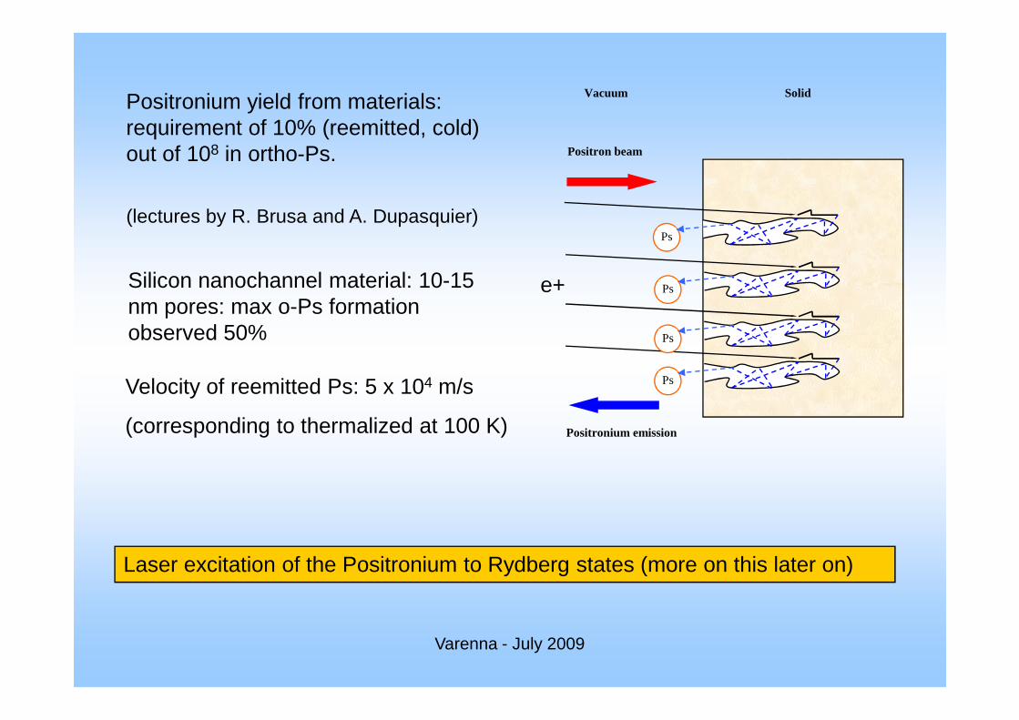
Positronium yield from materials: requirement of 10% (reemitted, cold) out of 108 in ortho-Ps.
(lectures by R. Brusa and A. Dupasquier)
Silicon nanochannel material: 10-15 nm pores: max o-Ps formation observed 50%
Varenna - July 2009
Ps
Positronium emission
Velocity of reemitted Ps: 5 x 10⁴ m/s
(corresponding to thermalized at 100 K)
Laser excitation of the Positronium to Rydberg states (more on this later on)

Ultracold Antiprotons
•The CERN AD (Antiproton Decelerator) delivers 3 x 10⁷ antiprotons / 80 sec
•Antiprotons catching in cylindrical Penning traps after energy degrader
•Catching of antiprotons within a 3 Tesla magnetic field, UHV, 4 Kelvin, e- cooling
•Stacking several AD shots
Antiprotons
Production GeV
Deceleration MeV
Trapping keV
Cooling eV
Varenna - July 2009
•Stacking several AD shots (104/105 subeV antiprotons)
•Transfer in the Antihydrogen formation region (1 Tesla, 100 mK)
•Cooling antiprotons down to 100 mK
•105 antiprotons ready for Antihydrogen production
• Resistive cooling based on high-Q resonant circuits
• Sympathetic cooling with laser cooled Os- ions
U. Warring et al., PRL 102 (2009) 043001

A E g I S in short
Acceleration of antihydrogen.
Formation of antihydrogen atoms
The antihydrogen beams will fly (with v~500 m/sec) through a Moire’ deflectometer
•Positronium: 107 atoms
•Antiprotons: 105
Varenna - July 2009
Such measurement would represent the first direct d etermination of the gravitational effect on antimat ter
Antiprotons
Positrons
The vertical displacement (gravity fall) will be measured on the last (sensitive) plane of the deflectometer
•Antihydrogen: 104/shot

Antihydrogen detector
How do we know that this works?
Intermediate level: need to know that we are producint Antihydrogen!
Ps*
e+ Bunch
cm1≈
Ps converter
Antiprotons
Varenna - July 2009
Antiproton Catching Zone (3 T)
Antihydrogen Formation Zone (1 T)
Deflectometer
Silicon microstrips
CsIcrystals
511 keV γ
511 keV γπ
π
π
Antihydrogen monitor

GOALVertex from tracking of charged particlesIdentification of 511 keV gammasTime and space coincidence of tracks + gammas
192 CsI (pure)Crystals
DESIGNCompact (radial thickness ~ 3 cm, length ~ 25 cm)Large solid angle (~ 80 %)High granularityOperation at T ~ 140 K, B = 3 Tesla
The Athena Anti-hydrogen detector
Varenna - July 2009
2 Layers of Si strips (r, φφφφ) and pads (z)
Time Resolution ~ 5 µs (CsI decay time ~ 1 µs)
Space Resolution ~ 4 mm (Vertex reconstruction σ )C. Regenfus, NIM A 501, 65 (2003).
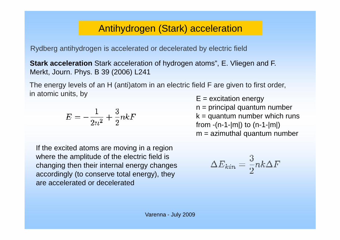
Antihydrogen (Stark) acceleration
Stark acceleration Stark acceleration of hydrogen atoms”, E. Vliegen and F. Merkt, Journ. Phys. B 39 (2006) L241
Rydberg antihydrogen is accelerated or decelerated by electric field
The energy levels of an H (anti)atom in an electric field F are given to first order, in atomic units, by
E = excitation energyn = principal quantum numberk = quantum number which runs
Varenna - July 2009
from -(n-1-|m|) to (n-1-|m|)m = azimuthal quantum number
If the excited atoms are moving in a region where the amplitude of the electric field is changing then their internal energy changes accordingly (to conserve total energy), they are accelerated or decelerated

- electric fields of few 100 V/cm are used (limited by field ionization)
- ∆v of few 100 m/s within about 1 cm can be achieved
Horizontal velocity (m/s)
Ato
ms
(1/m
s-1
)
no acceleration
acceleration
Varenna - July 2009
Effect of the magnetic field (e.g. 1 T)
n’ = quantum number which runs from -(n-1)/2, -(n-3)/2 to (n-3)/2, (n-1)/2γ = magnetic field in atomic units
Horizontal velocity (m/s)
accelerationaccelerationinside 1T
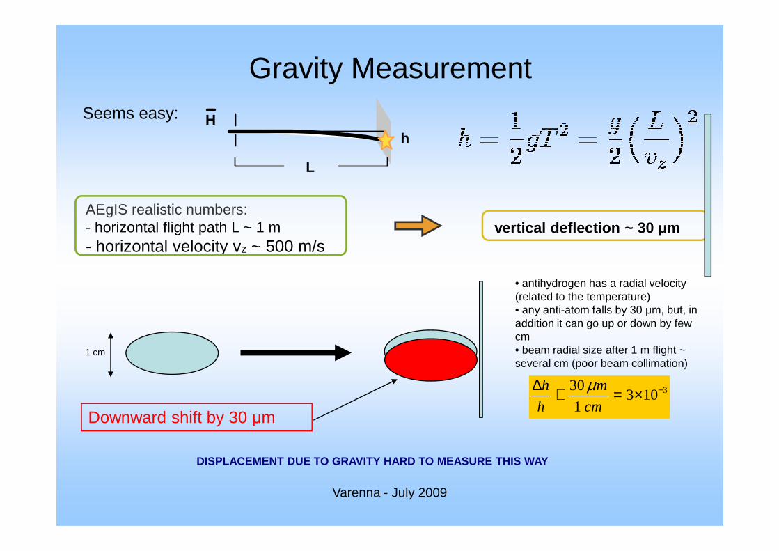
Gravity MeasurementSeems easy:
L
hH
AEgIS realistic numbers:- horizontal flight path L ~ 1 m- horizontal velocity vz ~ 500 m/s
vertical deflection ~ 30 µm
Varenna - July 2009
DISPLACEMENT DUE TO GRAVITY HARD TO MEASURE THIS WA Y
• antihydrogen has a radial velocity (related to the temperature)• any anti-atom falls by 30 µm, but, in addition it can go up or down by few cm• beam radial size after 1 m flight ~ several cm (poor beam collimation)
1 cm
Downward shift by 30 µm
3303 10
1
h m
h cm
µ −∆ ≅ = ×
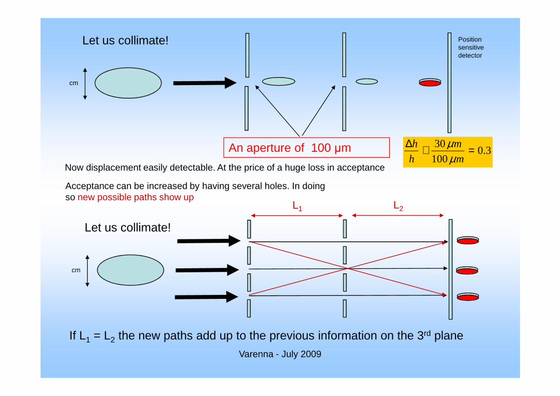
An aperture of 100 µm 300.3
100
h m
h m
µµ
∆ ≅ =Now displacement easily detectable. At the price of a huge loss in acceptance
cm
Let us collimate! Position sensitive detector
Acceptance can be increased by having several holes. In doing so new possible paths show up
Varenna - July 2009
so new possible paths show up
cm
Let us collimate!
L1 L2
If L1 = L2 the new paths add up to the previous information on the 3rd plane
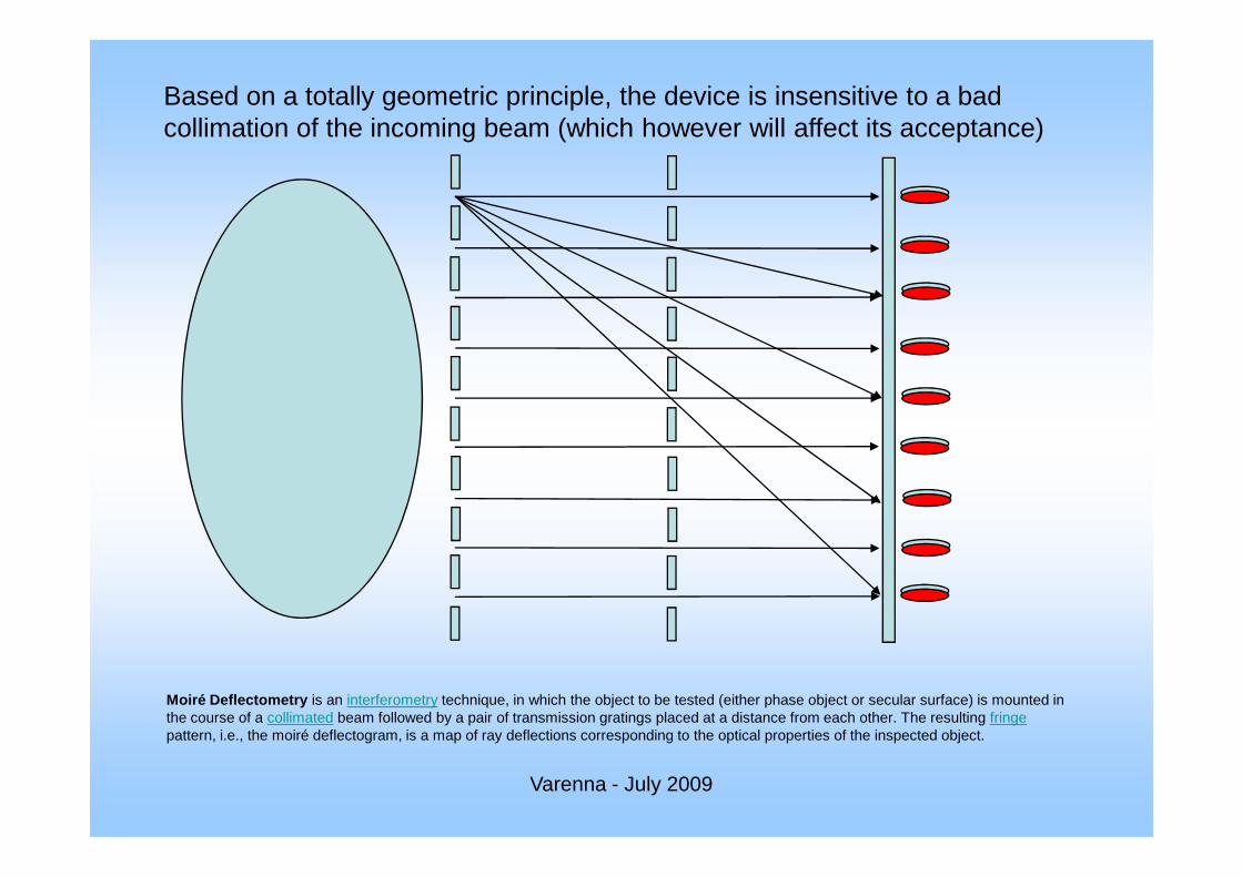
Based on a totally geometric principle, the device is insensitive to a bad collimation of the incoming beam (which however will affect its acceptance)
Varenna - July 2009
Moiré Deflectometry is an interferometry technique, in which the object to be tested (either phase object or secular surface) is mounted in the course of a collimated beam followed by a pair of transmission gratings placed at a distance from each other. The resulting fringepattern, i.e., the moiré deflectogram, is a map of ray deflections corresponding to the optical properties of the inspected object.

The final plane will be made of Silicon Strip detectors with a spatial resolution of about 10-15 µm
Now, this is NOT a quantum deflectometer, because:
Varenna - July 2009
So, it is a classical device if dg>> 10 µm
yg
hp
d≅
dgα
g
htg
d pα ≈
L gg
hL d
d p<< 2
g
hL d
p<<
2dB gL dλ <<
10dBL mλ µ≈
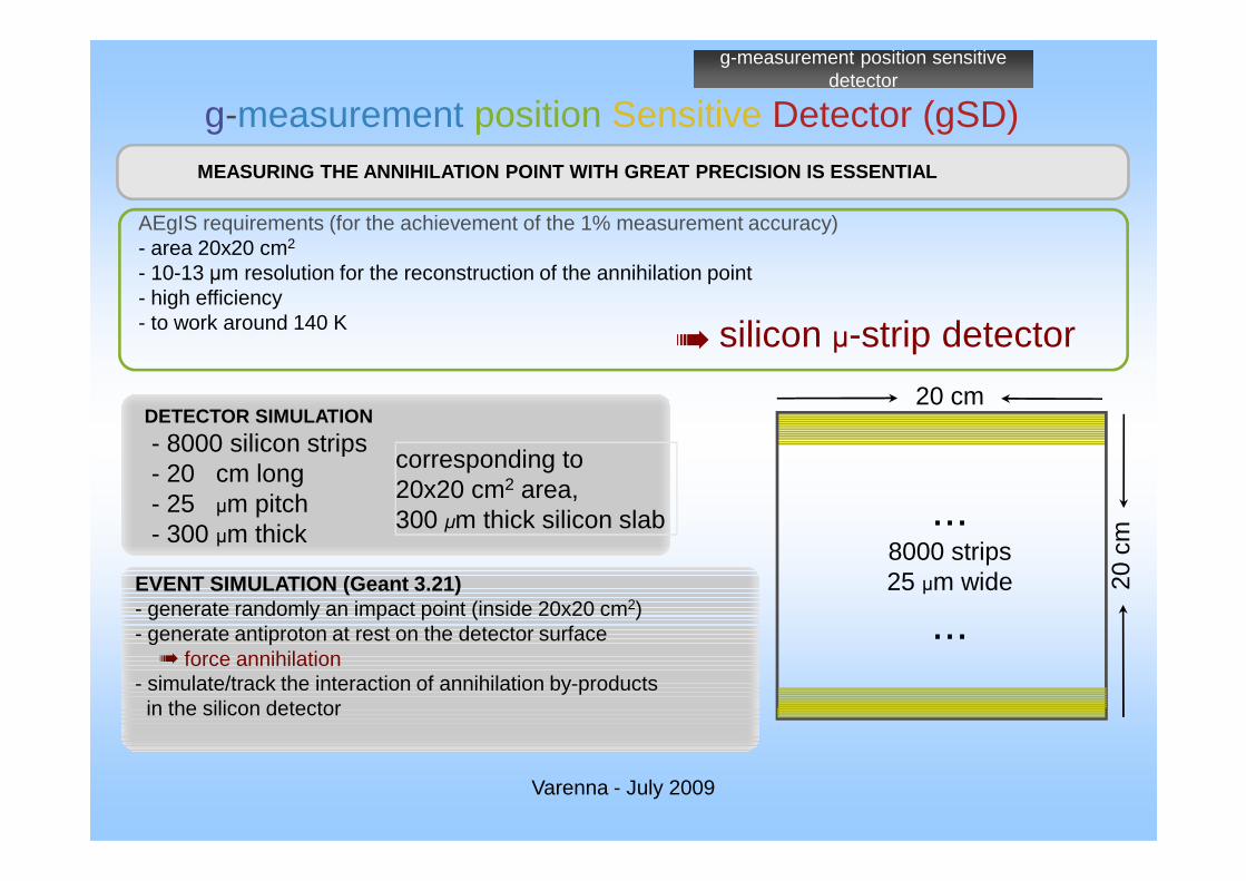
AEgIS requirements (for the achievement of the 1% measurement accuracy)- area 20x20 cm2
- 10-13 µm resolution for the reconstruction of the annihilation point- high efficiency- to work around 140 K
g-measurement position Sensitive Detector (gSD)MEASURING THE ANNIHILATION POINT WITH GREAT PRECISI ON IS ESSENTIAL
DETECTOR SIMULATION
- 8000 silicon strips
20 cm
g-measurement position sensitive detector
➠ silicon µ-strip detector
Varenna - July 2009
EVENT SIMULATION (Geant 3.21)- generate randomly an impact point (inside 20x20 cm2)- generate antiproton at rest on the detector surface ➠ force annihilation
- simulate/track the interaction of annihilation by-products in the silicon detector
- 8000 silicon strips- 20 cm long- 25 µm pitch- 300 µm thick
corresponding to 20x20 cm2 area, 300 µm thick silicon slab ...
8000 strips25 µm wide
...
20 c
m

annihilation hit position on the final detector(in a units)
grat
ing
slits
sha
dow
1
0
1
2
3
4
5
(x/a
)
annihilation hit position on the final detector
beam horizontal velocity
vz = 600 m/svz = 250 m/s
M o i r é deflectometerSuppose:- L = 40 cm- grating period a = 80 µm- grating size = 20 cm (2500 slits)- gravity
X
ZGrating transparency = 30%
(total transmission 9%)
moiré deflectometer
frin
ge s
hift
Varenna - July 2009
counts (a.u.)
grat
ing
slits
sha
dow
]a
-5
-4
-
3
-2
-
1
0
1
2
3
4
5
detector(in a units, modulo grating period a)
0 0.25 0.5 0.75 1 x/a
coun
ts (
a.u.
)
solidslit slit
frin
ge s
hift
Fringe shift !
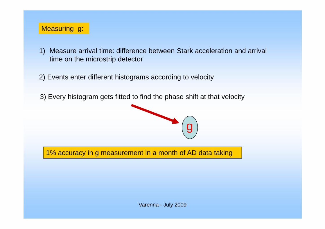
Measuring g:
1) Measure arrival time: difference between Stark acceleration and arrival time on the microstrip detector
2) Events enter different histograms according to velocity
3) Every histogram gets fitted to find the phase shift at that velocity
Varenna - July 2009
g
1% accuracy in g measurement in a month of AD data taking
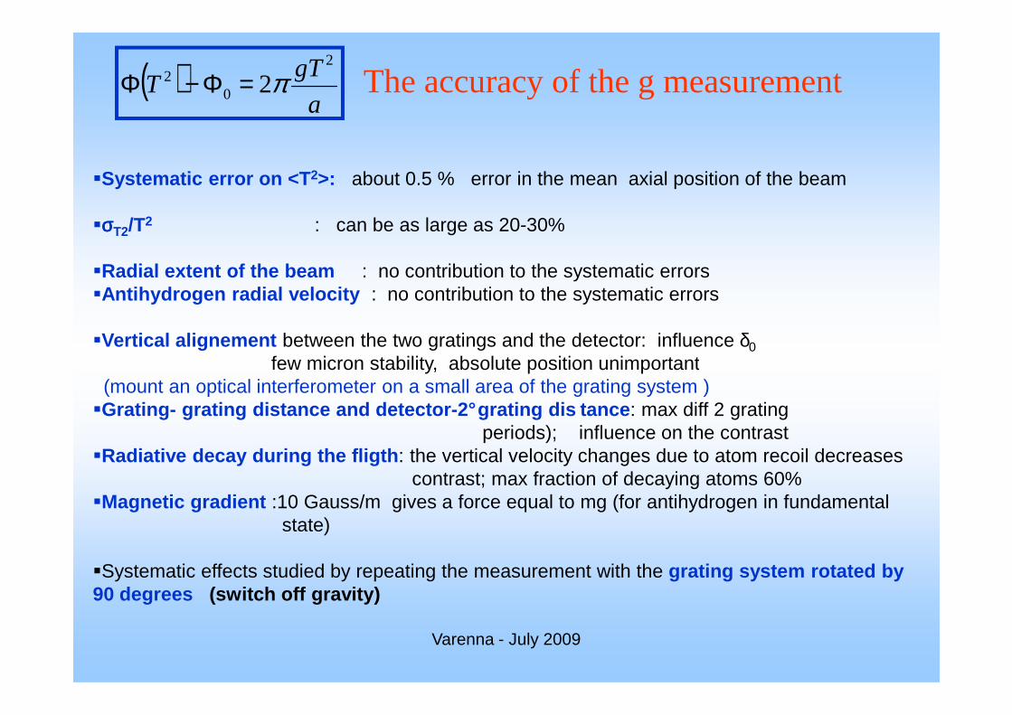
The accuracy of the g measurement
�Systematic error on <T 2>: about 0.5 % error in the mean axial position of the beam
�σσσσT2/T2 : can be as large as 20-30%
�Radial extent of the beam : no contribution to the systematic errors�Antihydrogen radial velocity : no contribution to the systematic errors
�Vertical alignement between the two gratings and the detector: influence δ0few micron stability, absolute position unimportant
( )a
gTT
2
02 2π=Φ−Φ
Varenna - July 2009
few micron stability, absolute position unimportant(mount an optical interferometer on a small area of the grating system )
�Grating- grating distance and detector-2°grating dis tance : max diff 2 grating periods); influence on the contrast
�Radiative decay during the fligth : the vertical velocity changes due to atom recoil decreases contrast; max fraction of decaying atoms 60%
�Magnetic gradient :10 Gauss/m gives a force equal to mg (for antihydrogen in fundamental state)
�Systematic effects studied by repeating the measurement with the grating system rotated by 90 degrees (switch off gravity)

M o i r é deflectometer
fringe shift of the shadow image
T = time of flight = [tSTARK - tDET] (L~ 1 m, v ~ 500 m/s ➠➠➠➠T ~ 2 ms )
Out beam is not monochromatic (T varies quite a lot)
v
coun
ts (
a.u.
)
m/s
Binning antihydrogens with mean velocity of 600-550-500-450-400-350-300-250-200 m/s,
and plotting δ as a function of ➠➠ ➠➠
Varenna - July 2009
m/s➠➠ ➠➠
coun
ts (
a.u.
)
ms 2
T2
δ (
a.u.
)
time of flight T (s)
g comes from the fit

Now, before moving on to more serious problems, we would like to thank the organizers for this pleasant time here
Varenna - July 2009
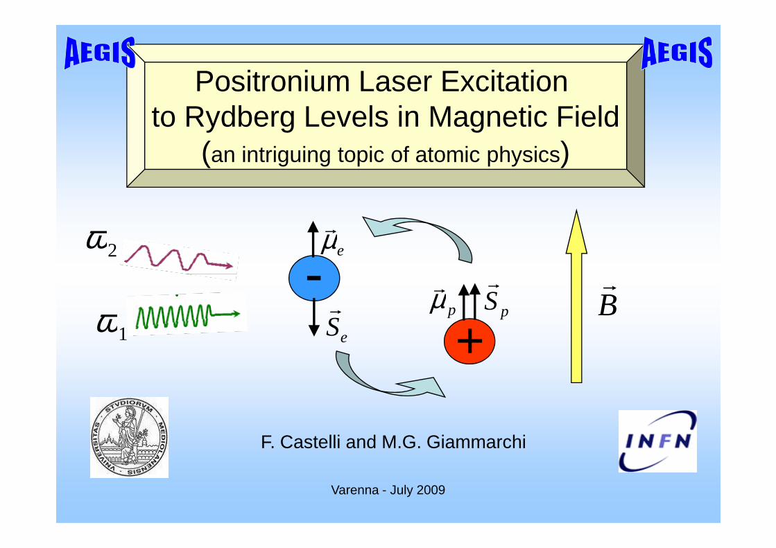
Positronium Laser Excitation to Rydberg Levels in Magnetic Field
(an intriguing topic of atomic physics)
-eµr2ω
Varenna - July 2009
-eSr
+pSr
pµr Br
1ω
F. Castelli and M.G. Giammarchi
Outline
The structure of Positronium (Ps) energy levels in magnetic fields♫ Experiments and theory: only n = 1,2 and weak fields♫ Moving Ps in strong magnetic fields:
♪ Zeeman and diamagnetic effects♪ motional Stark effect – the most effective!
♫ Energy splitting and mixing of n-sublevels, physical consequences
Varenna - July 2009
Efficient Ps laser excitation to high- n (Rydberg) levels: tailoring of laser pulses for maximizing the efficiency
♫ Two possible paths of excitation with two laser pulse♫ Line broadening: Doppler and motional Stark effects♫ Theory of incoherent excitation and determination of saturation fluence♫ Laser pulses energy and bandwidth, efficiency ♫ Modeling of excitation dynamics and Conclusions
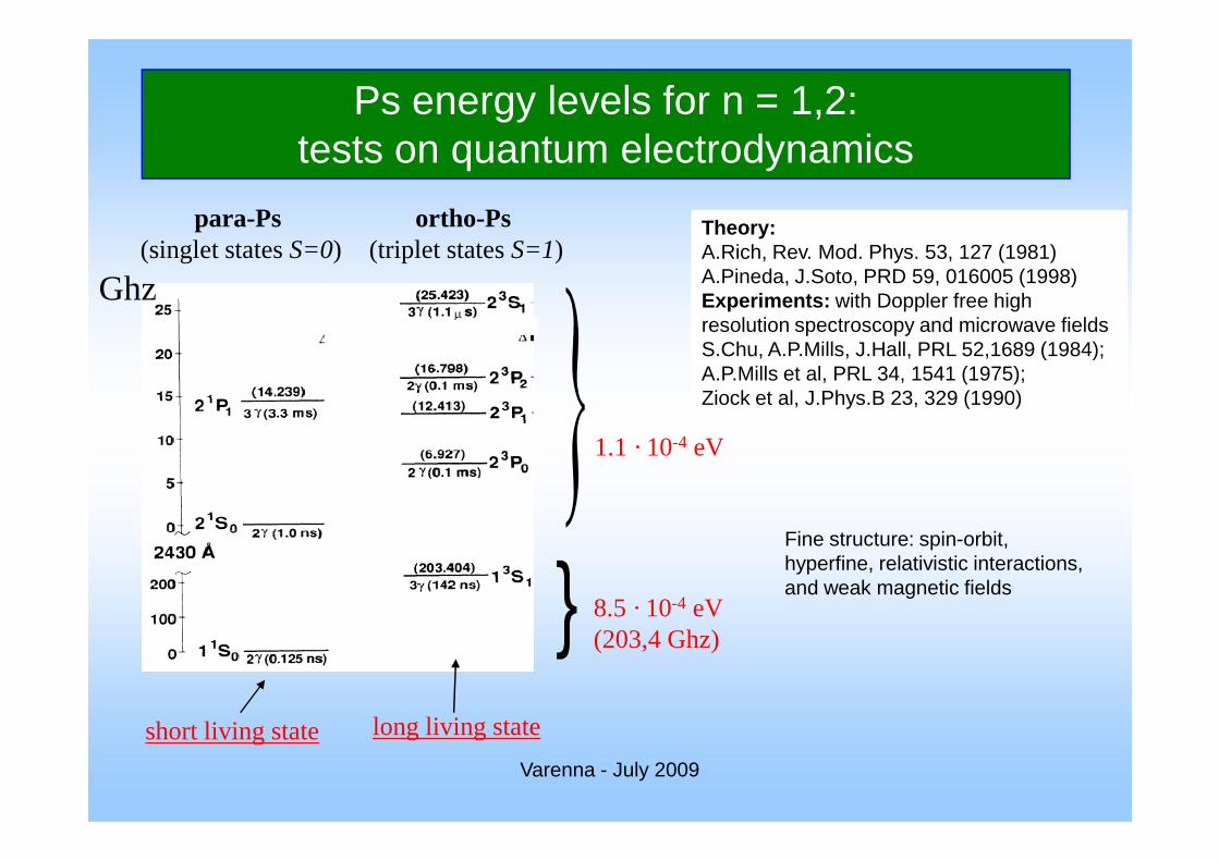
para-Ps (singlet states S=0)
ortho-Ps(triplet states S=1)
Ghz
Ps energy levels for n = 1,2: tests on quantum electrodynamics
Theory:A.Rich, Rev. Mod. Phys. 53, 127 (1981)A.Pineda, J.Soto, PRD 59, 016005 (1998)Experiments: with Doppler free high resolution spectroscopy and microwave fieldsS.Chu, A.P.Mills, J.Hall, PRL 52,1689 (1984);A.P.Mills et al, PRL 34, 1541 (1975);Ziock et al, J.Phys.B 23, 329 (1990)
Varenna - July 2009
} 8.5 · 10-4 eV(203,4 Ghz)
1.1 · 10-4 eV
long living stateshort living state
Fine structure: spin-orbit, hyperfine, relativistic interactions,and weak magnetic fields
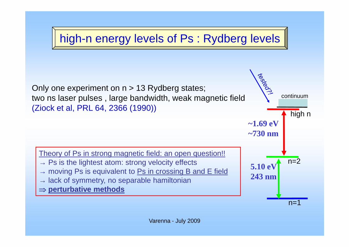
high-n energy levels of Ps : Rydberg levels
Only one experiment on n > 13 Rydberg states;two ns laser pulses , large bandwidth, weak magnetic field(Ziock et al, PRL 64, 2366 (1990))
continuum
high n~1.69 eV
Varenna - July 2009
n=2
n=1
5.10 eV243 nm
~1.69 eV~730 nm
Theory of Ps in strong magnetic field: an open question!!→ Ps is the lightest atom: strong velocity effects→ moving Ps is equivalent to Ps in crossing B and E field→ lack of symmetry, no separable hamiltonian⇒⇒⇒⇒ perturbative methods
two particles with Coulomb interaction diamagnetic
8764444 84444 76rvvelocitywithrestatPs
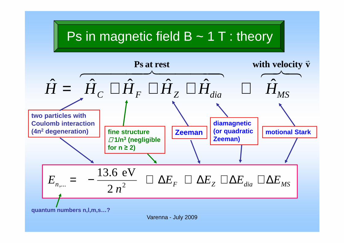
MSdiaZFC HHHHHH ˆˆˆˆˆˆ ++++=
Ps in magnetic field B ~ 1 T : theory
Varenna - July 2009
MSdiaZFn EEEEn
E ∆+∆+∆+∆+−=2,... 2
eV6.13
Coulomb interaction (4n2 degeneration) Zeeman motional Stark
diamagnetic(or quadratic Zeeman)
fine structure ∝∝∝∝ 1/n3 (negligible for n ≥ 2)
quantum numbers n,l,m,s…?
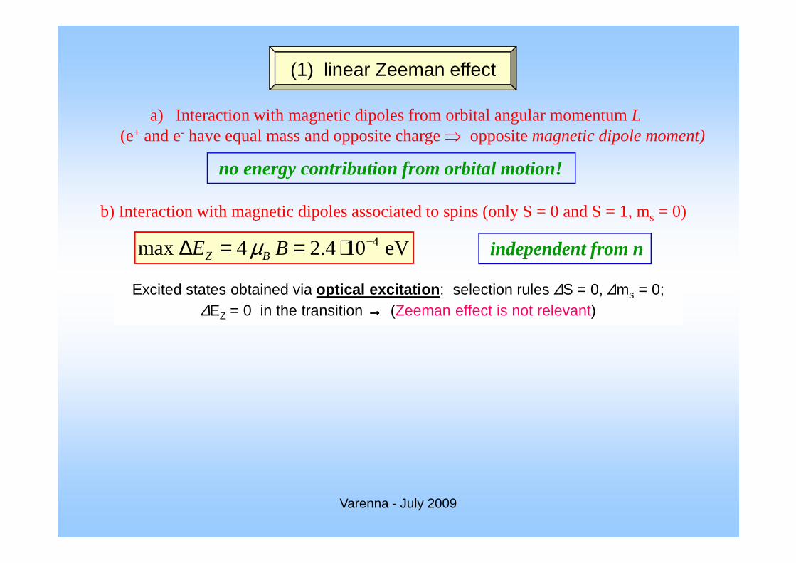
a) Interaction with magnetic dipoles from orbital angular momentum L(e+ and e- have equal mass and opposite charge ⇒ oppositemagnetic dipole moment)
(1) linear Zeeman effect
b) Interaction with magnetic dipoles associated to spins (only S = 0 and S = 1, ms = 0)
no energy contribution from orbital motion!
eV104.24max 4−⋅==∆ BE BZ µ independent from n
Excited states obtained via optical excitation : selection rules ∆S = 0, ∆m = 0;
Varenna - July 2009
Excited states obtained via optical excitation : selection rules ∆S = 0, ∆ms = 0;∆EZ = 0 in the transition →→→→ (Zeeman effect is not relevant)
(1) linear Zeeman effect
b) Interaction with magnetic dipoles associated to spins (only S = 0 and S = 1, ms = 0)
no energy contribution from orbital motion!
eV104.24max 4−⋅==∆ BE BZ µ independent from n
Excited states obtained via optical excitation : selection rules ∆S = 0, ∆m = 0;
a) Interaction with magnetic dipoles from orbital angular momentum L(e+ and e- have equal mass and opposite charge ⇒ oppositemagnetic dipole moment)
Varenna - July 2009
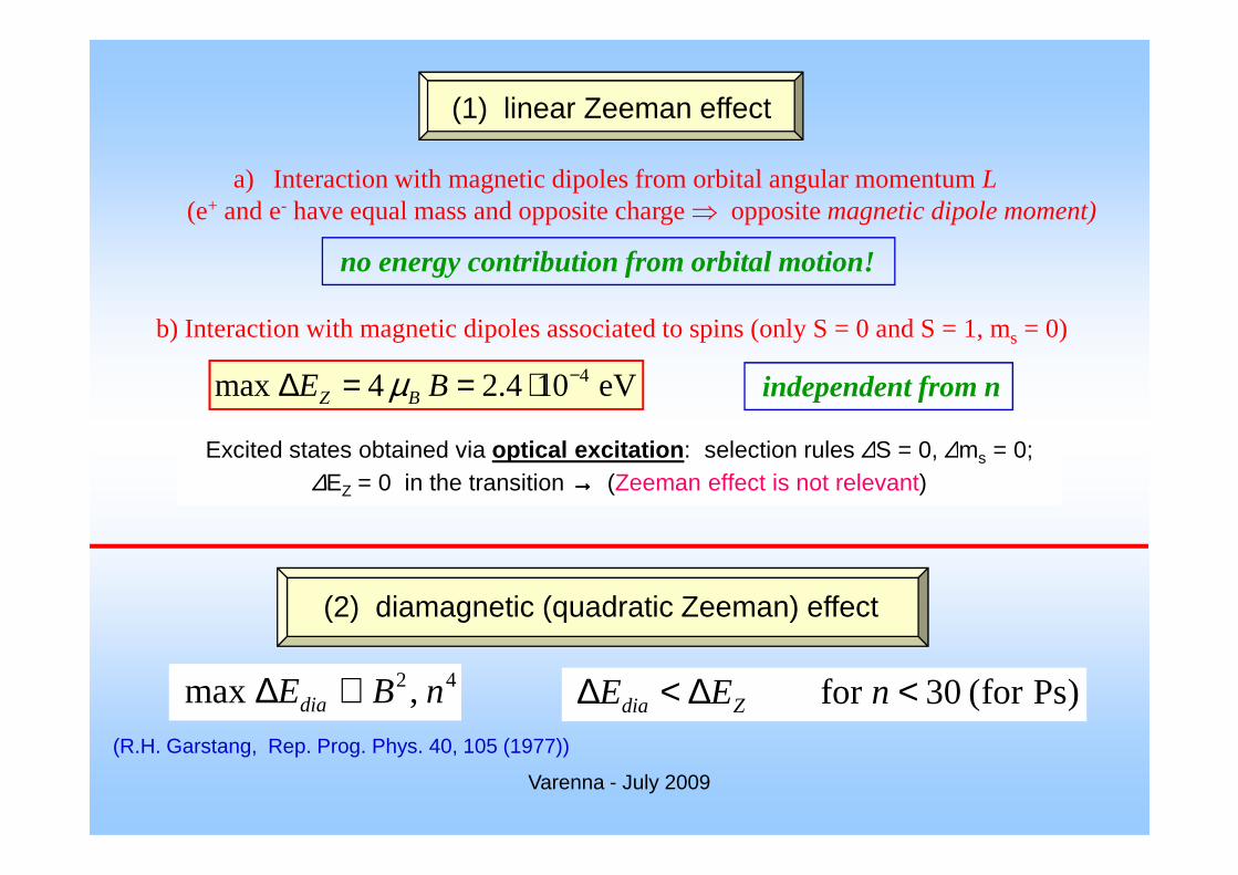
(R.H. Garstang, Rep. Prog. Phys. 40, 105 (1977))
42,max nBEdia ∝∆ )Psfor(30for <∆<∆ nEE Zdia
(2) diamagnetic (quadratic Zeeman) effect
Excited states obtained via optical excitation : selection rules ∆S = 0, ∆ms = 0;∆EZ = 0 in the transition →→→→ (Zeeman effect is not relevant)

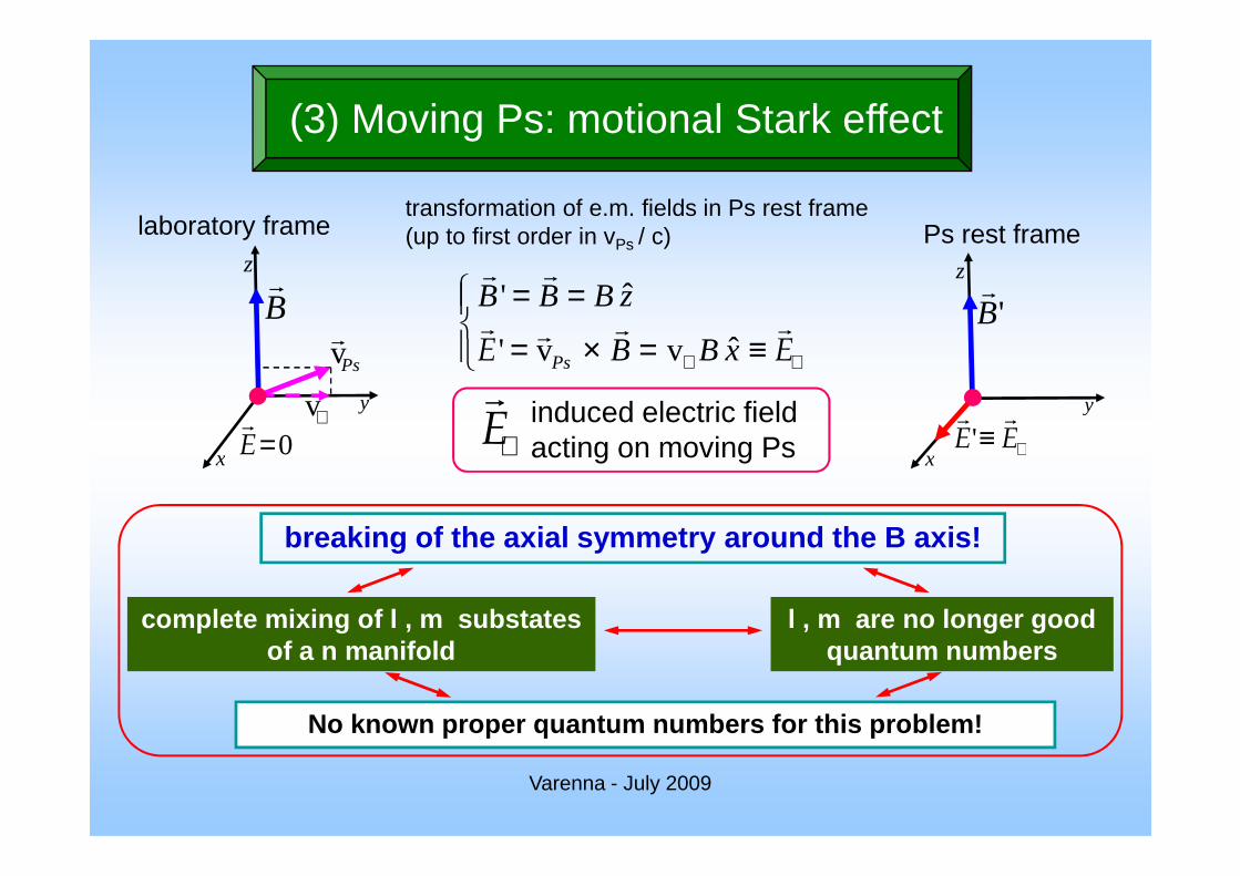
(3) Moving Ps: motional Stark effect
⊥≡ EE
rr'
'Br
z
y
Ps rest framelaboratory frame
≡=×=
==
⊥⊥ EE
rrrr
rr
xBB
zBBB
Ps ˆvv'
ˆ'
transformation of e.m. fields in Ps rest frame (up to first order in vPs / c)
Br
Psvr
z
y⊥v
0=Er
Varenna - July 2009
⊥≡ EE'xx 0=E
(3) Moving Ps: motional Stark effect
⊥≡ EE
rr'
'Br
z
y
Ps rest framelaboratory frame
≡=×=
==
⊥⊥ EE
rrrr
rr
xBB
zBBB
Ps ˆvv'
ˆ'
transformation of e.m. fields in Ps rest frame (up to first order in vPs / c)
Br
Psvr
z
y⊥v
0=Er
⊥Er
induced electric field acting on moving Ps
Varenna - July 2009
⊥≡ EE'xx 0=E
breaking of the axial symmetry around the B axis!
complete mixing of l , m substatesof a n manifold
l , m are no longer good quantum numbers
No known proper quantum numbers for this problem!
⊥E acting on moving Ps
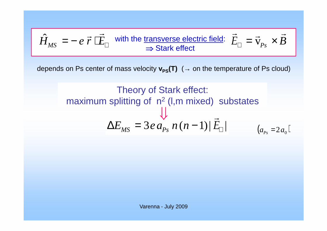
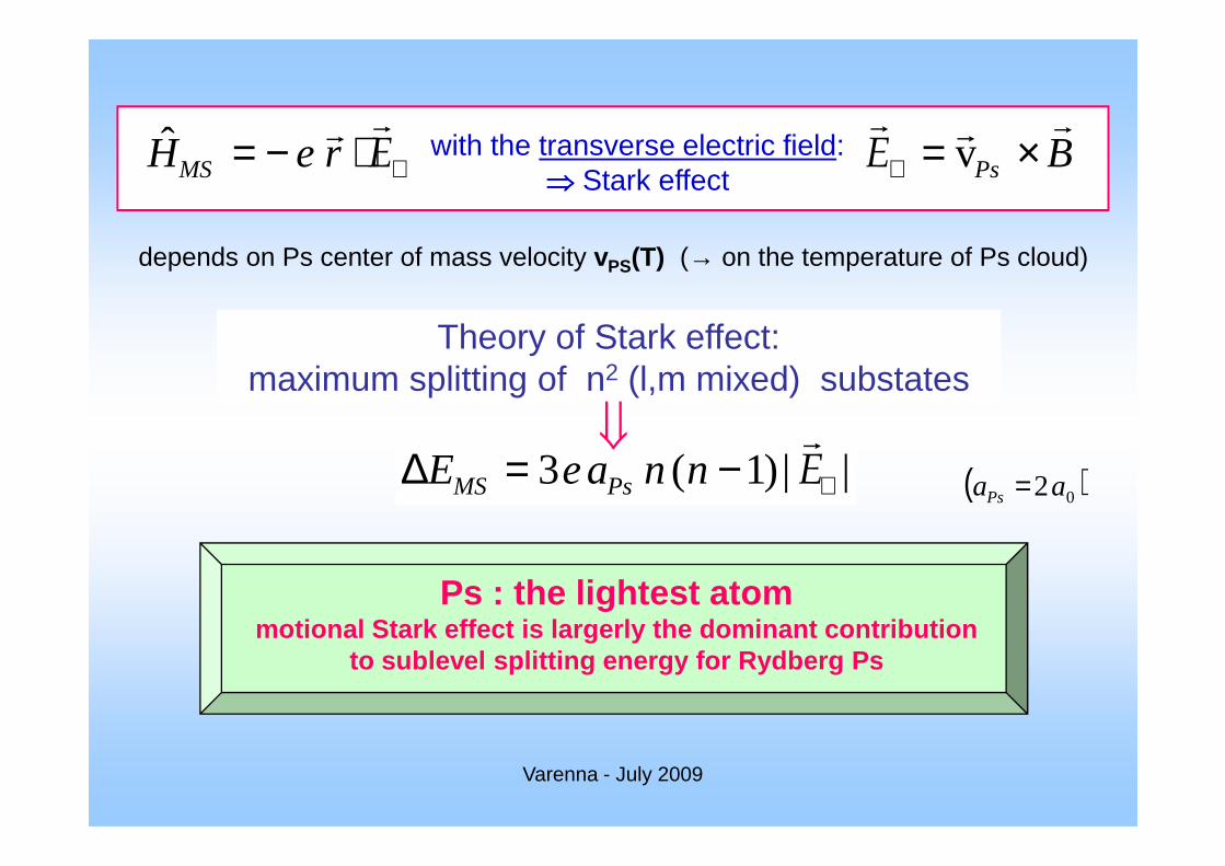
with the transverse electric field:⇒⇒⇒⇒ Stark effect⊥⋅−= Ε
rrreHMS
ˆ BPs
rrr×=⊥ vE
depends on Ps center of mass velocity vPS(T) (→ on the temperature of Ps cloud)
Theory of Stark effect:maximum splitting of n2 (l,m mixed) substates
⇓
Varenna - July 2009
||)1(3 ⊥−=∆ Er
nnaeE PsMS ( )02aaPs =⇓
with the transverse electric field:⇒⇒⇒⇒ Stark effect⊥⋅−= Ε
rrreHMS
ˆ BPs
rrr×=⊥ vE
depends on Ps center of mass velocity vPS(T) (→ on the temperature of Ps cloud)
Theory of Stark effect:maximum splitting of n2 (l,m mixed) substates
⇓
Varenna - July 2009
||)1(3 ⊥−=∆ Er
nnaeE PsMS ( )02aaPs =⇓
Ps : the lightest atommotional Stark effect is largerly the dominant cont ribution
to sublevel splitting energy for Rydberg Ps
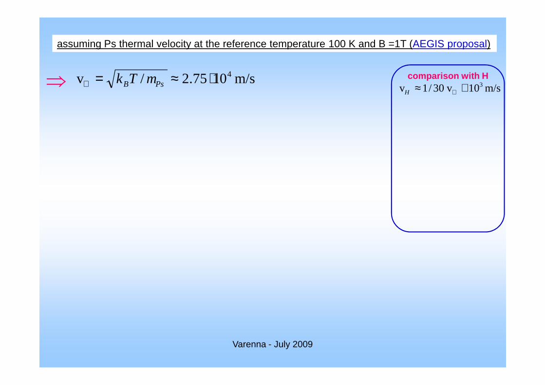
m/s1075.2/v 4⋅≈=⊥ PsB mTk
assuming Ps thermal velocity at the reference temperature 100 K and B =1T (AEGIS proposal)
⇒ m/s10v30/1v 3≅≈ ⊥H
comparison with H
Varenna - July 2009
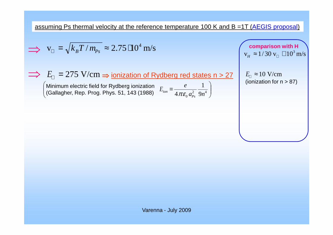
m/s1075.2/v 4⋅≈=⊥ PsB mTk
assuming Ps thermal velocity at the reference temperature 100 K and B =1T (AEGIS proposal)
⇒⇒⇒⇒ ionization of Rydberg red states n > 27V/cm275=⊥E
= 42
0 91
4 na
e
Psion επE
Minimum electric field for Rydberg ionization (Gallagher, Rep. Prog. Phys. 51, 143 (1988)
⇒
⇒
m/s10v30/1v 3≅≈ ⊥H
V/cm10≈⊥E
(ionization for n > 87)
comparison with H
Varenna - July 2009

m/s1075.2/v 4⋅≈=⊥ PsB mTk
assuming Ps thermal velocity at the reference temperature 100 K and B =1T (AEGIS proposal)
⇒⇒⇒⇒ ionization of Rydberg red states n > 27V/cm275=⊥E
= 42
0 91
4 na
e
Psion επE
Minimum electric field for Rydberg ionization (Gallagher, Rep. Prog. Phys. 51, 143 (1988)
diaZMS EEE ∆∆>>∆ ,
⇒
⇒
⇒ for n > 6
m/s10v30/1v 3≅≈ ⊥H
comparison with H
V/cm10≈⊥E
(ionization for n > 87)
diaMSZ EEE ∆∆>∆ ,for n < 40
Varenna - July 2009
diaZMS EEE ∆∆>>∆ ,⇒ for n > 6
nMSdia EEE ∆>∆>∆for n > 46
m/s1075.2/v 4⋅≈=⊥ PsB mTk
assuming Ps thermal velocity at the reference temperature 100 K and B =1T (AEGIS proposal)
⇒⇒⇒⇒ ionization of Rydberg red states n > 27V/cm275=⊥E
= 42
0 91
4 na
e
Psion επE
Minimum electric field for Rydberg ionization (Gallagher, Rep. Prog. Phys. 51, 143 (1988)
diaZMS EEE ∆∆>>∆ ,
⇒
⇒
⇒ for n > 6
m/s10v30/1v 3≅≈ ⊥H
comparison with H atoms
V/cm10≈⊥E
(ionization for n > 87)
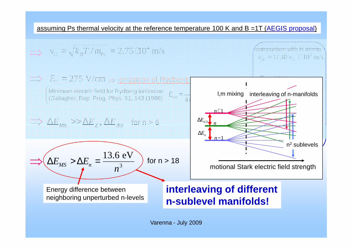
diaMSZ EEE ∆∆>∆ ,for n < 401+∆ nE
1+n
n
l,m mixing interleaving of n-manifolds
Varenna - July 2009
diaZMS EEE ∆∆>>∆ ,⇒
3
eV6.13
nEE nMS =∆>∆
Energy difference between neighboring unperturbed n-levels
for n > 6
for n > 18
interleaving of different n-sublevel manifolds!
⇒
nMSdia EEE ∆>∆>∆for n > 46
nE∆
n
1−n
motional Stark electric field strength
n2 sublevels
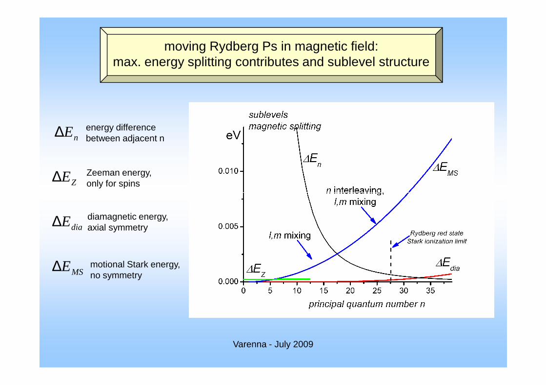
moving Rydberg Ps in magnetic field:max. energy splitting contributes and sublevel structure
Z
n
E
E
∆
∆ energy difference between adjacent n
Zeeman energy, only for spins
Varenna - July 2009
MS
dia
E
E
∆
∆ diamagnetic energy, axial symmetry
motional Stark energy, no symmetry

motional Stark effect
� strong mixing of of n-manifolds containing n2 sub-states
� optical resonance line broadening ?
� no l,m quantum numbers → no electric dipole selection rules forinteraction with e.m. radiation → all sublevels interacting
weak dependence on T and B
Varenna - July 2009
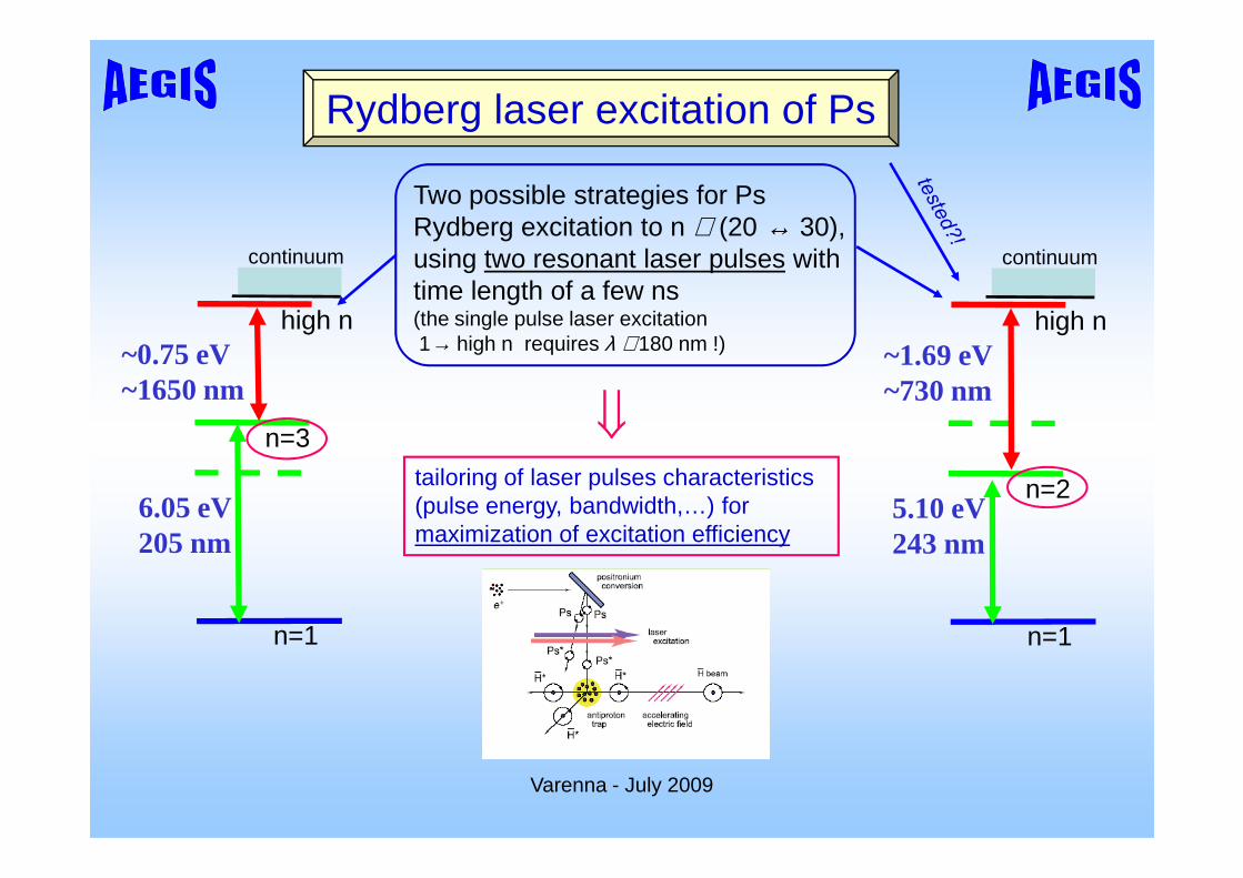
Rydberg laser excitation of Ps
continuum
high n~1.69 eV~730 nm
n=3
continuum
high n~0.75 eV~1650 nm
Two possible strategies for Ps Rydberg excitation to n ∈ (20 ↔ 30), using two resonant laser pulses with time length of a few ns(the single pulse laser excitation1→ high n requires λ ≅ 180 nm !)
⇓
Varenna - July 2009
n=2
n=1
5.10 eV243 nm
n=3
n=1
6.05 eV205 nm
tailoring of laser pulses characteristics (pulse energy, bandwidth,…) for maximization of excitation efficiency
⇓
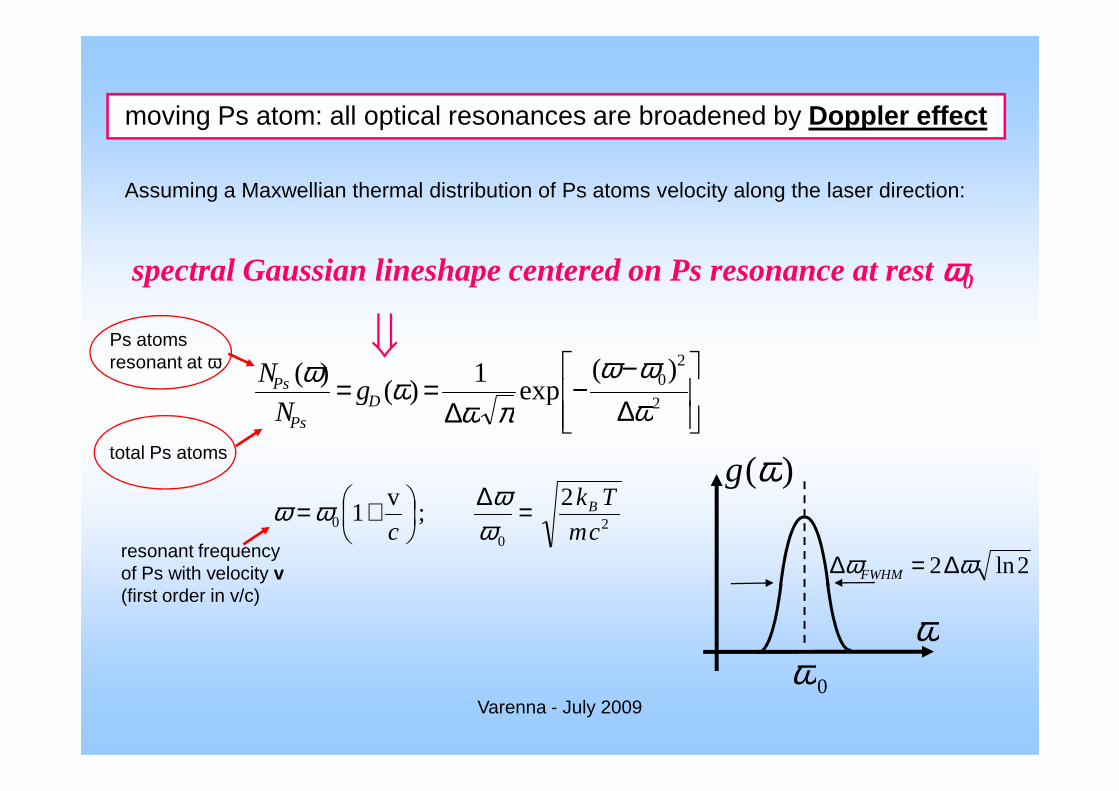
spectral Gaussian lineshape centered on Ps resonance at rest ωωωω0
∆−
−∆
== 2
20)(
exp1
)()(
ωωω
πωωω
DPs g
N
Assuming a Maxwellian thermal distribution of Ps atoms velocity along the laser direction:
Ps atoms resonant at ω ⇓
moving Ps atom: all optical resonances are broadened by Doppler effect
Varenna - July 2009
∆−
∆== 2exp)(
ωπωωD
Ps
gN
20
0
2;
v1
cm
Tk
cB=∆
+=ω
ωωω
0ω
)(ωg
ω
2ln2 ωω ∆=∆ FWHM
total Ps atoms
resonant frequency of Ps with velocity v(first order in v/c)
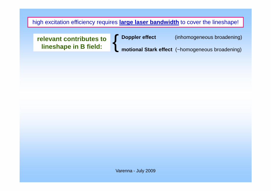
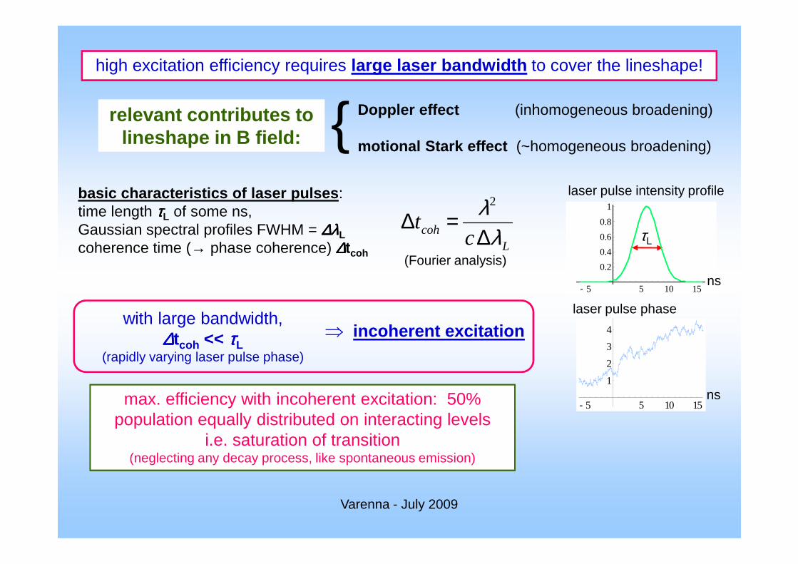
relevant contributes to lineshape in B field: {Doppler effect (inhomogeneous broadening)
motional Stark effect (~homogeneous broadening)
high excitation efficiency requires large laser bandwidth to cover the lineshape!
Varenna - July 2009

Lcoh c
tλ
λ∆
=∆2
basic characteristics of laser pulses : time length ττττL of some ns,Gaussian spectral profiles FWHM = ∆λ∆λ∆λ∆λLcoherence time (→ phase coherence) ∆∆∆∆tcoh
(Fourier analysis)
relevant contributes to lineshape in B field: {Doppler effect (inhomogeneous broadening)
motional Stark effect (~homogeneous broadening)
0.2
0.4
0.6
0.8
1
laser pulse intensity profile
ns
τL
high excitation efficiency requires large laser bandwidth to cover the lineshape!
Varenna - July 2009
- 5 5 10 15
- 5 5 10 15
1
2
3
4
laser pulse phase
ns
ns
Lcoh c
tλ
λ∆
=∆2
basic characteristics of laser pulses : time length ττττL of some ns,Gaussian spectral profiles FWHM = ∆λ∆λ∆λ∆λLcoherence time (→ phase coherence) ∆∆∆∆tcoh
(Fourier analysis)
high excitation efficiency requires large laser bandwidth to cover the lineshape!
relevant contributes to lineshape in B field: {Doppler effect (inhomogeneous broadening)
motional Stark effect (~homogeneous broadening)
0.2
0.4
0.6
0.8
1
laser pulse intensity profile
ns
τL
Varenna - July 2009
with large bandwidth, ∆∆∆∆tcoh << ττττL
(rapidly varying laser pulse phase)
⇒ incoherent excitation
- 5 5 10 15
- 5 5 10 15
1
2
3
4
laser pulse phase
ns
nsmax. efficiency with incoherent excitation: 50%population equally distributed on interacting levels
i.e. saturation of transition(neglecting any decay process, like spontaneous emission)
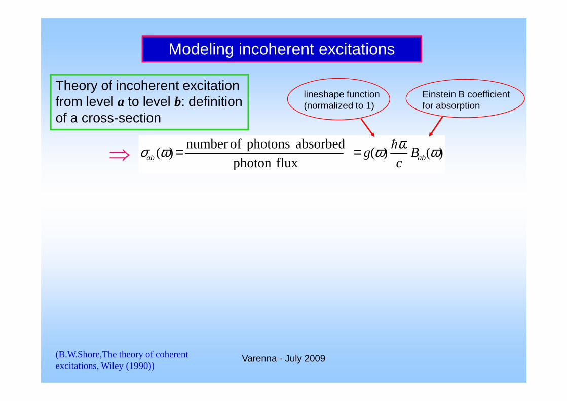
Modeling incoherent excitations
)()(fluxphoton
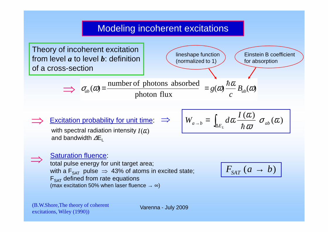
absorbedphotonsofnumber )( ωωωωσ abab B
cg
h==
Theory of incoherent excitation from level a to level b: definition of a cross-section
⇒
Einstein B coefficient for absorption
lineshape function (normalized to 1)
Varenna - July 2009(B.W.Shore,The theory of coherent excitations, Wiley (1990))
Modeling incoherent excitations
)()( ωσωω I
dW ∫=⇒⇒
)()(fluxphoton
absorbedphotonsofnumber )( ωωωωσ abab B
cg
h==
Theory of incoherent excitation from level a to level b: definition of a cross-section
⇒
Einstein B coefficient for absorption
lineshape function (normalized to 1)
Varenna - July 2009
)(ωI
)()( ωσ
ωωω abEba
IdW
L h∫∆→ =Excitation probability for unit time:with spectral radiation intensityand bandwidth ∆EL
⇒⇒
Saturation fluence: total pulse energy for unit target area;with a FSAT pulse ⇒ 43% of atoms in excited state;FSAT defined from rate equations(max excitation 50% when laser fluence → ∞)
)( baFSAT →
(B.W.Shore,The theory of coherent excitations, Wiley (1990))
⇒
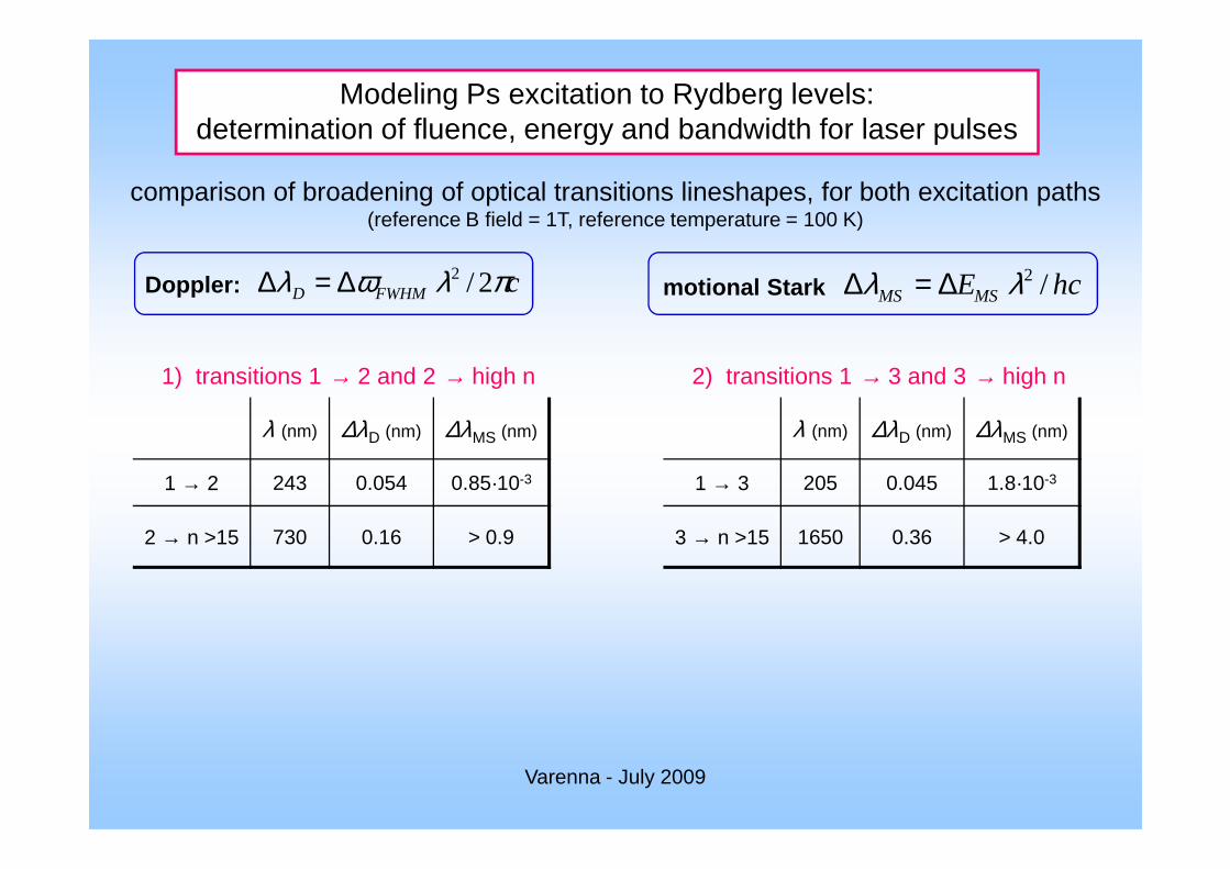
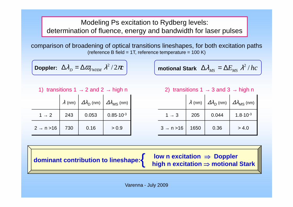
Modeling Ps excitation to Rydberg levels:determination of fluence, energy and bandwidth for laser pulses
1) transitions 1 → 2 and 2 → high n
comparison of broadening of optical transitions lineshapes, for both excitation paths(reference B field = 1T, reference temperature = 100 K)
hcEMSMS /2λλ ∆=∆motional StarkDoppler: cFWHMD πλωλ 2/2∆=∆
2) transitions 1 → 3 and 3 → high n
λ (nm) ∆λD (nm) ∆λMS (nm) λ (nm) ∆λD (nm) ∆λMS (nm)
Varenna - July 2009
λ (nm) ∆λD (nm) ∆λMS (nm)
1 → 2 243 0.054 0.85·10-3
2 → n >15 730 0.16 > 0.9
λ (nm) ∆λD (nm) ∆λMS (nm)
1 → 3 205 0.045 1.8·10-3
3 → n >15 1650 0.36 > 4.0
1) transitions 1 → 2 and 2 → high n
comparison of broadening of optical transitions lineshapes, for both excitation paths(reference B field = 1T, reference temperature = 100 K)
hcEMSMS /2λλ ∆=∆motional StarkDoppler: cFWHMD πλωλ 2/2∆=∆
2) transitions 1 → 3 and 3 → high n
λ (nm) ∆λD (nm) ∆λMS (nm) λ (nm) ∆λD (nm) ∆λMS (nm)
Modeling Ps excitation to Rydberg levels:determination of fluence, energy and bandwidth for laser pulses
Varenna - July 2009
low n excitation ⇒⇒⇒⇒ Doppler high n excitation ⇒⇒⇒⇒ motional Stark
dominant contribution to lineshape: {
λ (nm) ∆λD (nm) ∆λMS (nm)
1 → 2 243 0.053 0.85·10-3
2 → n >16 730 0.16 > 0.9
λ (nm) ∆λD (nm) ∆λMS (nm)
1 → 3 205 0.044 1.8·10-3
3 → n >16 1650 0.36 > 4.0
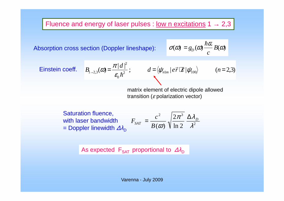
Fluence and energy of laser pulses : low n excitations 1 → 2,3
)()()( ωωωωσ Bc
gD
h=Absorption cross section (Doppler lineshape):
Einstein coeff. )3,2(||;||
)( 100120
2
3,21 =⋅==→ nredd
B mn ψεψε
πω rr
h
matrix element of electric dipole allowed transition (ε polarization vector)
Varenna - July 2009
Saturation fluence,with laser bandwidth = Doppler linewidth ∆λD
2
32
2ln
2
)( λλπ
ωD
SAT B
cF
∆=
As expected FSAT proportional to ∆λD
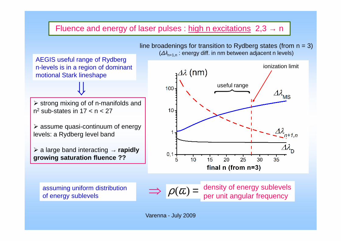
Fluence and energy of laser pulses : high n excitations 2,3 → n
AEGIS useful range of Rydberg n-levels is in a region of dominant motional Stark lineshape
ionization limit
line broadenings for transition to Rydberg states (from n = 3)(∆λn+1,n : energy diff. in nm between adjacent n levels)
}useful range
� strong mixing of of n-manifolds and n2 sub-states in 17 < n < 27
⇓
Varenna - July 2009
� assume quasi-continuum of energy levels: a Rydberg level band
� a large band interacting → rapidly growing saturation fluence ??
assuming uniform distribution of energy sublevels ⇒ =)(ωρ density of energy sublevels
per unit angular frequency
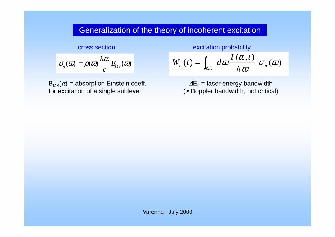
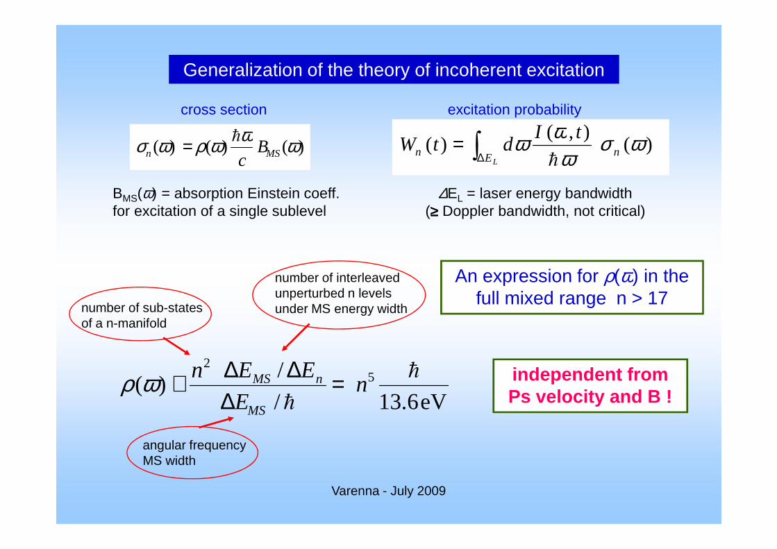
Generalization of the theory of incoherent excitation
)()()( ωωωρωσ MSn Bc
h= )(),(
)( ωσω
ωω nEn
tIdtW
L h∫∆=
cross section excitation probability
∆EL = laser energy bandwidth (≥≥≥≥ Doppler bandwidth, not critical)
BMS(ω) = absorption Einstein coeff. for excitation of a single sublevel
Varenna - July 2009
Generalization of the theory of incoherent excitation
)()()( ωωωρωσ MSn Bc
h=
number of interleaved An expression for ρ(ω) in the
)(),(
)( ωσω
ωω nEn
tIdtW
L h∫∆=
cross section excitation probability
∆EL = laser energy bandwidth (≥≥≥≥ Doppler bandwidth, not critical)
BMS(ω) = absorption Einstein coeff. for excitation of a single sublevel
Varenna - July 2009
eV6.13/
/)( 5
2 h
hn
E
EEn
MS
nMS =∆
∆∆≅ωρ
number of interleaved unperturbed n levels under MS energy widthnumber of sub-states
of a n-manifold
angular frequency MS width
An expression for ρ(ω) in the full mixed range n > 17
independent from Ps velocity and B !
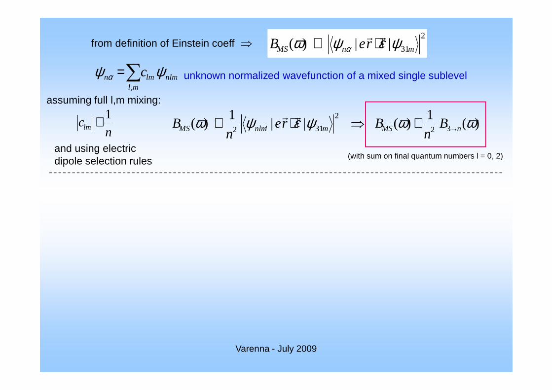
2
31||)( mnMS reB ψεψω αrr⋅∝from definition of Einstein coeff ⇒
unknown normalized wavefunction of a mixed single sublevel∑=ml
nlmlmn c,
ψψ α
assuming full l,m mixing:
nclm
1≅ )(1
)(||1
)( 32
2
31'2ωωψεψω nMSmnlmMS B
nBre
nB →≅⇒⋅∝
rr
and using electric dipole selection rules (with sum on final quantum numbers l = 0, 2)
Varenna - July 2009
Scaling of BMS coefficient and excitation probability
2
31||)( mnMS reB ψεψω αrr⋅∝from definition of Einstein coeff ⇒
unknown normalized wavefunction of a mixed single sublevel∑=ml
nlmlmn c,
ψψ α
assuming full l,m mixing:
nclm
1≅ )(1
)(||1
)( 32
2
31'2ωωψεψω nMSmnlmMS B
nBre
nB →≅⇒⋅∝
rr
and using electric dipole selection rules (with sum on final quantum numbers l = 0, 2)
Varenna - July 2009
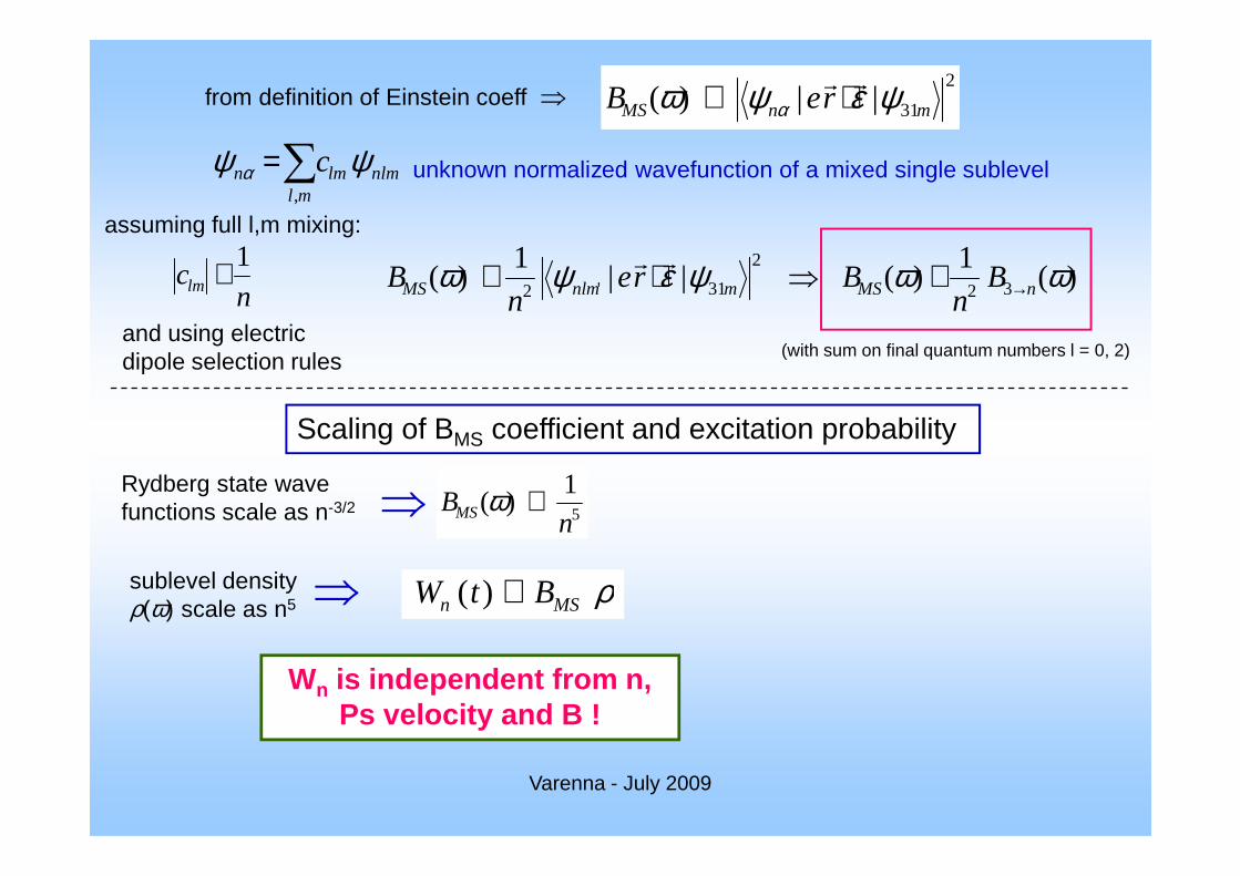
Scaling of BMS coefficient and excitation probability
Rydberg state wave functions scale as n-3/2 ⇒ 5
1)(
nBMS ∝ω
sublevel density ρ(ω) scale as n5 ⇒ ρMSn BtW ∝)(
Wn is independent from n, Ps velocity and B !
Scaling of BMS coefficient and excitation probability
2
31||)( mnMS reB ψεψω αrr⋅∝from definition of Einstein coeff ⇒
unknown normalized wavefunction of a mixed single sublevel∑=ml
nlmlmn c,
ψψ α
assuming full l,m mixing:
nclm
1≅ )(1
)(||1
)( 32
2
31'2ωωψεψω nMSmnlmMS B
nBre
nB →≅⇒⋅∝
rr
and using electric dipole selection rules (with sum on final quantum numbers l = 0, 2)
Varenna - July 2009
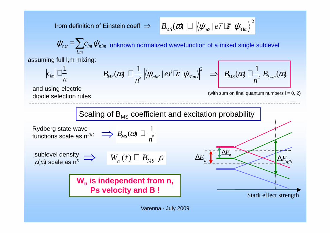
Scaling of BMS coefficient and excitation probability
Rydberg state wave functions scale as n-3/2 ⇒ 5
1)(
nBMS ∝ω
sublevel density ρ(ω) scale as n5
strengtheffect Stark
MSE∆LE∆ nE∆⇒ ρMSn BtW ∝)(
Wn is independent from n, Ps velocity and B !
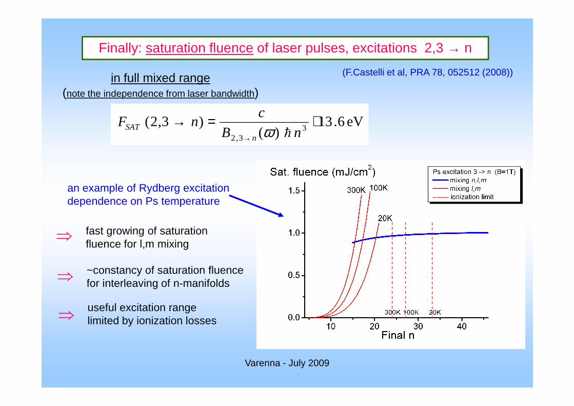
Finally: saturation fluence of laser pulses, excitations 2,3 → n
in full mixed range(note the independence from laser bandwidth)
eV6.13)(
)3,2( 33,2
⋅=→→ nB
cnF
nSAT
hω
(F.Castelli et al, PRA 78, 052512 (2008))
an example of Rydberg excitation dependence on Ps temperature
Varenna - July 2009
fast growing of saturation fluence for l,m mixing
~constancy of saturation fluence for interleaving of n-manifolds
useful excitation range limited by ionization losses
dependence on Ps temperature
⇒
⇒
⇒
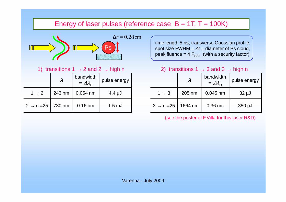
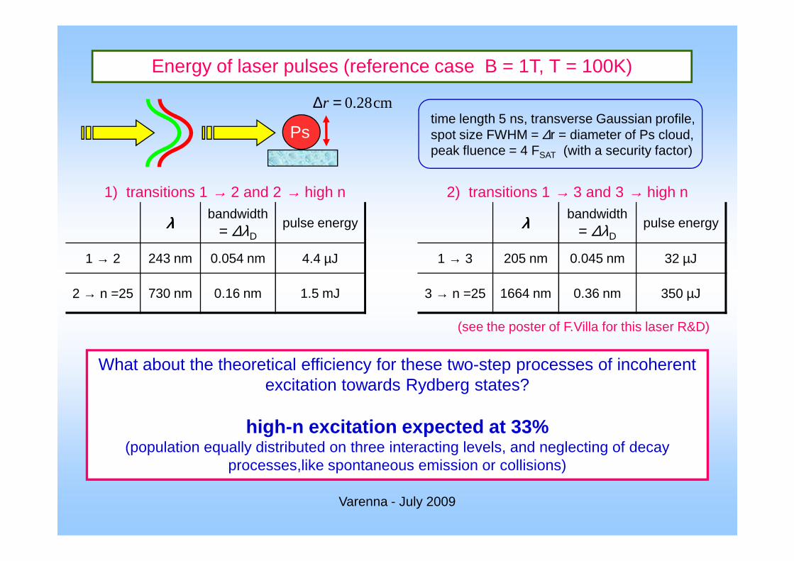
Ps
cm28.0=∆rtime length 5 ns, transverse Gaussian profile, spot size FWHM = ∆r = diameter of Ps cloud,peak fluence = 4 FSAT (with a security factor)
λλλλ bandwidth = ∆λD
pulse energy
1 → 2 243 nm 0.054 nm 4.4 µJ
Energy of laser pulses (reference case B = 1T, T = 100K)
λλλλ bandwidth = ∆λD
pulse energy
1 → 3 205 nm 0.045 nm 32 µJ
1) transitions 1 → 2 and 2 → high n 2) transitions 1 → 3 and 3 → high n
Varenna - July 2009
2 → n =25 730 nm 0.16 nm 1.5 mJ 3 → n =25 1664 nm 0.36 nm 350 µJ
(see the poster of F.Villa for this laser R&D)
Ps
cm28.0=∆rtime length 5 ns, transverse Gaussian profile, spot size FWHM = ∆r = diameter of Ps cloud,peak fluence = 4 FSAT (with a security factor)
λλλλ bandwidth = ∆λD
pulse energy
1 → 2 243 nm 0.054 nm 4.4 µJ
Energy of laser pulses (reference case B = 1T, T = 100K)
λλλλ bandwidth = ∆λD
pulse energy
1 → 3 205 nm 0.045 nm 32 µJ
1) transitions 1 → 2 and 2 → high n 2) transitions 1 → 3 and 3 → high n
Varenna - July 2009
2 → n =25 730 nm 0.16 nm 1.5 mJ 3 → n =25 1664 nm 0.36 nm 350 µJ
What about the theoretical efficiency for these two-step processes of incoherent excitation towards Rydberg states?
high- n excitation expected at 33%(population equally distributed on three interacting levels, and neglecting of decay
processes,like spontaneous emission or collisions)
(see the poster of F.Villa for this laser R&D)
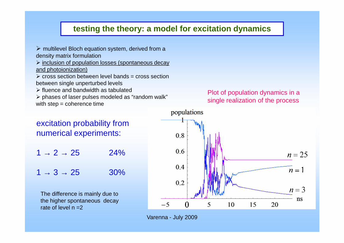
testing the theory: a model for excitation dynamics
� multilevel Bloch equation system, derived from a density matrix formulation� inclusion of population losses (spontaneous decay and photoionization)� cross section between level bands = cross section between single unperturbed levels� fluence and bandwidth as tabulated� phases of laser pulses modeled as “random walk” with step = coherence time
Plot of population dynamics in a single realization of the process
excitation probability from
Varenna - July 2009
excitation probability from numerical experiments:
1 → 2 → 25 24%
1 → 3 → 25 30%
The difference is mainly due to the higher spontaneous decay rate of level n =2
Conclusions♫ Development of a “first order” analysis of the energy level
structure of a moving Ps atom in magnetic field;♫ Formulation of a generalized theory of incoherent excitation,
for application in sublevel full mixing cases;♫ Determination of laser pulse characteristics, to the goal of
maximum efficiency in Ps excitation for AEGIS
Varenna - July 2009
Possible improvements♫ Detailed description of Ps energy levels;♫ Refinement of the incoherent excitation theory;♫ More realistic modelization of excitation dynamics♫ Experimental tests on Ps Rydberg excitation ?
Varenna - July 2009

Possible improvements♫ Detailed description of Ps energy levels;♫ Refinement of the incoherent excitation theory;♫ More realistic modelization of excitation dynamics♫ Experimental tests on Ps Rydberg excitation ?
Thanks to the organizers and …
next school?
Varenna - July 2009
next school?

Monte Carlo
Choice of the production point
Choice of velocity
Choice of grating characteristics
Tracking
Summing up the period of the grating
Varenna - July 2009
Reference model: L = 30 cm
Size of gratings : 20 x 20 cm2
Pitch of grating 100 µm
Opening fraction 30%
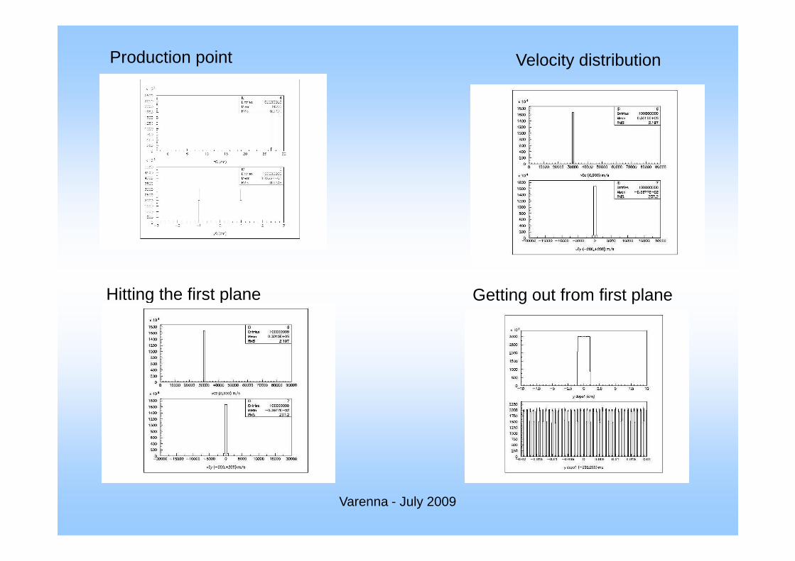
Production point Velocity distribution
Varenna - July 2009
Hitting the first plane Getting out from first plane
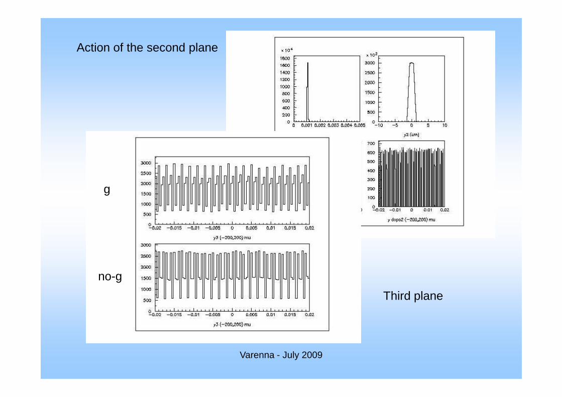
Action of the second plane
g
Varenna - July 2009
Third plane
no-g
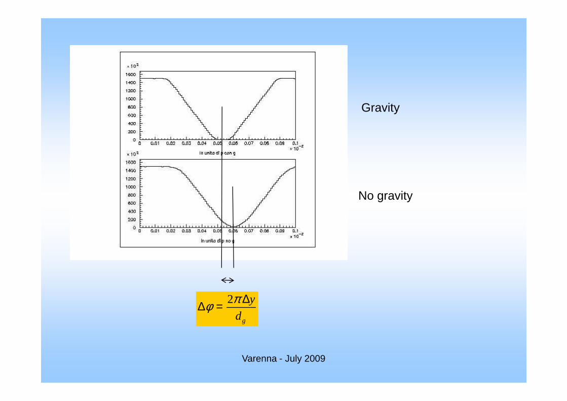
Gravity
No gravity
Varenna - July 2009
No gravity
2
g
y
d
πφ ∆∆ =
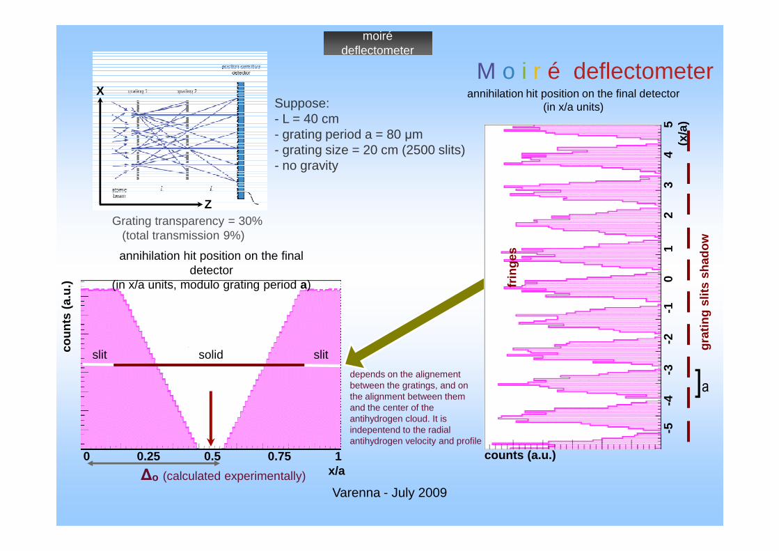
Suppose:- L = 40 cm- grating period a = 80 µm- grating size = 20 cm (2500 slits)- no gravity
M o i r é deflectometerX
ZGrating transparency = 30%
(total transmission 9%)
moiré deflectometer
annihilation hit position on the final detector
1
0
1
2
3
4
5
(x/a
)
annihilation hit position on the final detector(in x/a units)
grat
ing
slits
sha
dow
frin
ges
Varenna - July 2009∆o (calculated experimentally)
detector(in x/a units, modulo grating period a)
0 0.25 0.5 0.75 1 x/a
coun
ts (
a.u.
)
slit slitsolid
counts (a.u.)
]a
-5
-4
-
3
-2
-
1
0
1
2
3
4
5
grat
ing
slits
sha
dow
frin
ges
depends on the alignement between the gratings, and on the alignment between them and the center of the antihydrogen cloud. It is indepentend to the radial antihydrogen velocity and profile
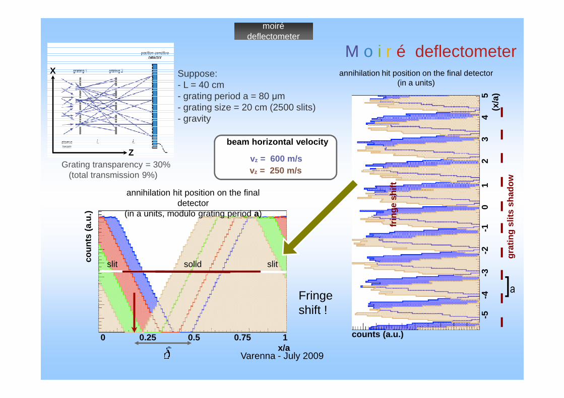
annihilation hit position on the final detector(in a units)
grat
ing
slits
sha
dow
1
0
1
2
3
4
5
(x/a
)
annihilation hit position on the final detector
beam horizontal velocity
vz = 600 m/svz = 250 m/s
M o i r é deflectometerSuppose:- L = 40 cm- grating period a = 80 µm- grating size = 20 cm (2500 slits)- gravity
X
ZGrating transparency = 30%
(total transmission 9%)
moiré deflectometer
frin
ge s
hift
Varenna - July 2009
counts (a.u.)
grat
ing
slits
sha
dow
]a
-5
-4
-
3
-2
-
1
0
1
2
3
4
5
detector(in a units, modulo grating period a)
0 0.25 0.5 0.75 1 x/a
coun
ts (
a.u.
)
solidslit slit
frin
ge s
hift
Fringe shift !
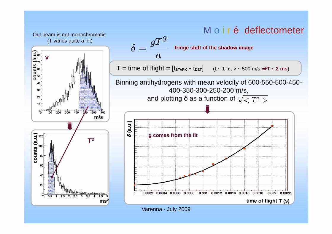
M o i r é deflectometer
fringe shift of the shadow image
T = time of flight = [tSTARK - tDET] (L~ 1 m, v ~ 500 m/s ➠➠➠➠T ~ 2 ms )
Out beam is not monochromatic (T varies quite a lot)
v
coun
ts (
a.u.
)
m/s
Binning antihydrogens with mean velocity of 600-550-500-450-400-350-300-250-200 m/s,
and plotting δ as a function of ➠➠ ➠➠
Varenna - July 2009
m/s➠➠ ➠➠
coun
ts (
a.u.
)
ms 2
T2
δ (
a.u.
)
time of flight T (s)
g comes from the fit