diploma thesis design and simulation of a flexible robotic
TRANSCRIPT

Athens, October 2019
NATIONAL TECHNICAL UNIVERSITY OF ATHENS
School of Mechanical Engineering
Manufacturing Technology Section
Diploma Thesis
Design and Simulation of a Flexible Robotic System
for Biotechnology Experiment Production
Angelidou Charikleia
Supervisors
G. - C. Vosniakos Professor, NTUA
P. Benardos Assistant Professor, NTUA

“The best preparation for tomorrow is doing your best today”
H. Jackson Brown Jr, (b. 1941)

i
ACKNOWLEDGEMENTS
This project and the work that came with it wouldn’t have been realized without the support
and guidance of many great people.
First of all I would like to thank professor Georgios C. Vosniakos for giving me the opportunity
to be part of his team and for turning this experience into more than a simple academic
project. Having been given the chance to collaborate directly with the industry, I acquired
valuable knowledge and skills. The interest and trust from his behalf have been major factors
towards the completion of this diploma thesis. His advisory and guidance meant a lot for me
and I highly appreciate it.
Moreover, I am grateful to have met and worked with assistant professor Panorios Benardos,
who was always keen on helping me overcome the difficulties that I encountered throughout
the project. His drive and his fresh view of things were very pleasant and enlightening.
I would also like to address a sincere thank you towards the people of experoment, a team of
young innovators, for trusting me with a project of their start-up and especially thank Imperial
College PhD candidate Francesco Cursi, for devoting his time to helping, advising and
supporting me throughout my work, even though he was not obliged to.
Beside the people in academia, I would like to wholeheartedly thank my friends who have
always been supportive and helpful in their own unique way. I wouldn’t have been the person
I am without them.
Finally, I would like to express my gratitude to my parents for always believing in me and for
providing me with their valuable support and love throughout my studies, as well as to my
siblings, who are always there for me, even though distance keeps us apart, and to whom I
want to dedicate this diploma thesis.
ii
ABSTRACT
The intent to accelerate scientific research on biotechnology has been increasing for the last
few decades drastically. Investing in novel ways of advancing this sector, utilizing the most up-
to date technological equipment, has therefore been in the center of attention. This is why
researchers and companies have started directing their attention towards automation and its
branches. Robotic cloud biotechnology laboratories constitute one of these branches, which
aim is to change the way research is done, dramatically offsetting the ever-increasing costs of
clinical trials, automating tedious lab work, and accelerating research by running experiments
in parallel, by making scientific testing efficient and programmable for all. An overview of the
design and function of such a robotic system is the central theme of the current project.
In the current thesis, studied are the methodology and tools for developing the virtual
equivalent of a real biotechnology laboratory for pharmaceutical experiments. Specifically, a
SCARA type robot, the Stäubli TX2-90XL robotic arm, as well as the lab environment, are
modeled using the 3D application development software VREP by Coppelia Robotics. The goal
is to investigate the offline programming of the arm in a virtual reality environment, as well
as to fully design a suitable lab layout that can be extrapolated on real-life laboratory settings.
As part of the design process, introduced are the components for the creation of the
laboratory set up, including equipment and consumables. Different laboratory layouts are
then created and compared, concluding to two specific set ups that are finally simulated.
For the modeling and simulation, the robot models are introduced and their respective
kinematic chains are developed. The forward and inverse kinematics of the arm are analyzed
and developed in Matlab, using different approaches and inverse algorithm methods such as
inverse and pseudo-inverse Jacobian, as well as the Damped Least Squares Method. The
trajectory of both robotic arms is planned so as to create a motion plan that can be used for
any experiment within the laboratory set ups. Additionally, a User Interface (UI) is created for
the communication of the experiment protocols between the researcher and the robotic
arms. Finally, two experiments are simulated for both robots and layouts.

iii

iv
Table of Contents
1 INTRODUCTION ................................................................................................................... 1
1.1 What is a Robotic Biotechnology Cloud Lab? ............................................................ 1
1.2 Digital Factory Technologies………………………………………………………………………… ........ 2
1.3 Efforts towards automated biotechnology labs ........................................................ 3
1.3.1 Existent Robotic Cloud Platforms ...................................................................... 3
1.4 Objectives and Goals of the Thesis Project………… .................................................. ..4
2 V-REP AND MATLAB INTERFACING .................................................................................. 6
2.1 Virtual Robot Experimentation Platform (V-REP) ...................................................... 6
2.1.1 Scene Object Types and Properties ................................................................... 6
2.1.2 Coordinate Systems ........................................................................................... 8
2.1.3 3D Model Import and Neutral File Formats .................................................... 10
2.2 Communication between MATLAB and the V-REP platform .................................. 11
2.3 Enabling the remote API…………………………………………………………………………………… .. 12
2.3.1 Client side activation ....................................................................................... 13
2.3.2 Server side activation ...................................................................................... 15
2.3.3 Basic Remote-API functions for MATLAB client .............................................. 16
3 THE ROBOTS ...................................................................................................................... 17
3.1 The custom SCARA robot of Experoment…. …………………………………………………………17
3.1.1 Description ...................................................................................................... 17
3.1.2 Advantages and limitations of SCARA robots .................................................. 19
3.2 Stäubli ΤX2-90XL………………………………………………. ................................................... 19
3.2.1 Description ...................................................................................................... 19
3.2.2 Advantages and limitations of 6-axis robots ................................................... 21
3.3 Robot 3D Model Import……………………………….. ....................................................... 21
3.3.1 Unified Robot Description Format (URDF) ...................................................... 22
3.3.2 Robot Coordinate Systems .............................................................................. 23
3.3.3 Scaling Factor ................................................................................................... 24
3.3.4 URDF and MATLAB Robotics Toolbox .............................................................. 24
3.4 Gripper Choice………………………………………………. ...................................................... 25
3.4.1 Parallel Grippers .............................................................................................. 26
4 LABORATORY EQUIPMENT................................................................................................. 28
4.1 Machines…………………………………………………….. ........................................................ 28

v
4.1.1 Liquid Handler ................................................................................................. 28
4.1.2 Centrifuge ........................................................................................................ 29
4.1.3 Freezer ............................................................................................................. 29
4.1.4 Incubator ......................................................................................................... 30
4.1.5 Plate Reader .................................................................................................... 30
4.2 Consumables……………………………………………………………………………………………………….31
5 LABORATORY STRUCTURE AND LAYOUTS .................................................................... 32
5.1 Flexible Manufacturing Systems (FMS)………………………. ......................................... 32
5.2 Production line layouts for FMS…………………………................................................... 32
5.2.1 Linear layout .................................................................................................... 33
5.2.2 Island (or Circular) Layout ............................................................................... 33
5.2.3 Vertical Ladder Layout ..................................................................................... 34
5.3 Laboratory Structure………………………………………………… ........................................... 35
6 KINEMATIC ANALYSIS OF MANIPULATORS .................................................................... 39
6.1 Introduction………………………………………………………. .................................................. 39
6.2 Kinematics………………………………………………………………………………………………….. ....... 39
6.2.1 Forward Kinematics ......................................................................................... 40
6.2.2 Joint Space and Operational Space ................................................................. 41
6.2.3 Inverse Kinematics ........................................................................................... 42
6.3 Differential Kinematics………………………………………………………….. .............................. 42
6.3.1 Geometric Jacobian ......................................................................................... 43
6.3.2 Inverse Differential Kinematics........................................................................ 44
6.3.3 Kinematic Singularities .................................................................................... 44
6.4 Inverse Kinematics Algorithms………………………………….. .......................................... 45
6.4.1 Inverse Jacobian .............................................................................................. 45
6.4.2 Pseudo-Inverse Jacobian ................................................................................. 46
6.4.3 Damped Least Squares (DLS) ........................................................................... 46
6.5 Trajectory Planning…………………………………………. ..................................................... 47
6.6 Implementation on Robotic Manipulators……….. .................................................... 50
7 SIMULATION ................................................................................................................... 55
7.1 Visual Simulation Models……………………………… ....................................................... 55
7.1.1 Robots .............................................................................................................. 55
7.1.2 Lab Equipment ................................................................................................. 56
7.1.3 Safe Positions................................................................................................... 57
7.1.4 Parameterization of the simulation................................................................. 57
7.2 Experiment Protocols………………………………….. ........................................................ 58

vi
7.3 User Interface ( UI )…………………………………….. ......................................................... 59
7.4 Simulation of Experiment with SCARA and STAUBLI ............................................... 60
7.4.1 SCARA .............................................................................................................. 60
7.4.2 STAUBLI TX2-90XL ............................................................................................ 62
7.5 Collision Detection……………………………………….. ....................................................... 64
8 RESULTS ........................................................................................................................... 66
8.1 General Remarks…………………………………………. ........................................................ 66
8.2 SCARA…………………………………………………………… ....................................................... 67
8.3 STAUBLI RX-90………………………………………………. ....................................................... 74
9 CONCLUSIONS AND FUTURE WORK ............................................................................... 78
9.1 Contribution…………………………………………………. ....................................................... 78
9.2 Advantages of virtual environments……….………… ................................................... 78
9.3 Suggestions for future development………………… ................................ …………………79
10 BIBLIOGRAPHY ............................................................................................................ 80
APPENDIX ................................................................................................................................ 82
A URDF Template[22]…………………………………………………. ................................................. - 1 -
B TECHNICAL SPECIFICATIONS OF EQUIPMENT AND CONSUMABLES ............................. - 6 -
C MATLAB CODE……………………………………………………. .................................................... - 13 -
SCARA FILES ................................................................................................................. - 13 -
STAUBLI FILES .............................................................................................................. - 42 -

vii
Figure Inventory
Figure 1: Section of web page of the experoment platform ..................................................... 4
Figure 2: Clockwise coordinate system ..................................................................................... 9
Figure 3: V-REP communication framework[8] ....................................................................... 11
Figure 4: Remote API functionality overview[8] ..................................................................... 12
Figure 5: MATLAB code for establishing and terminating communication with V-REP platform
................................................................................................................................................. 14
Figure 6: LUA code for server-side activation ......................................................................... 15
Figure 7: Workspace of SCARA type robot .............................................................................. 18
Figure 8: Stäubli TX2-90XL Robot ............................................................................................ 19
Figure 9: Working space of Staubli TX2-90XL [Source: Staubli] ........................................................ 20
Figure 10: Different mounting positions for Staubli TX2-90XL ............................................... 21
Figure 11: Link and joint representation ................................................................................. 22
Figure 12: Matlab code for importing URDF file ..................................................................... 24
Figure 13: Details for SCARA robot ......................................................................................... 25
Figure 14: Details for Staubli TX2-90XL ................................................................................... 25
Figure 15: Cell-carrier 96 on the left and Cell-carrier 384 on the right .................................. 31
Figure 16: Linear layout for production .................................................................................. 33
Figure 17: Island (or circular) layout for production ............................................................... 34
Figure 18: Vertical Ladder layout for production .................................................................... 35
Figure 19: Conventional representations of joints[17] ........................................................... 40
Figure 20: Description of the position and orientation of the end-effector frame[17] .......... 40
Figure 21: Calculation of Homogenous Transform T with Matlab Robotics Toolbox ............. 50
Figure 22: Calculation of Geometric Jacobian with Matlab Robotics Toolbox ....................... 52
Figure 23: Calculation of damping factor λ with SVD .............................................................. 52
Figure 24: Quadrating programming and solving of Inverse Kinematics with Matlab Robotics
Toolbox .................................................................................................................................... 53
Figure 25: Validation flowchart of kinematic model[21] ........................................................ 54
Figure 26: Robotic manager architecture ............................................................................... 54
Figure 27: Experiment protocol examples .............................................................................. 58
Figure 28: User interface flowchart ........................................................................................ 60

viii
Table Inventory
Table 1: Enabling the remote API-client side, Matlab documentation for simxStart function.
................................................................................................................................................. 14
Table 2: Enabling the remote API-client side, Matlab documentation for simxFinish function
................................................................................................................................................. 15
Table 3: Enabling the remote API –server side, LUA documentation for simRemoteApi.start
function ................................................................................................................................... 15
Table 4: Translational Joint Limits of the SCARA type robot ................................................... 18
Table 5: Rotary Joint Limits of the SCARA type robot ............................................................. 18
Table 6: Joint Limits of the Stäubli TX90XL.............................................................................. 20

ix
Diagram Inventory
Diagram 1: EE position of SCARA with FK- Home to Safe Position ......................................... 67
Diagram 2: Joint angles of SCARA with FK-Home to Safe Position ......................................... 67
Diagram 3: Joint velocities of SCARA with FK- Home to Safe Position ................................... 67
Diagram 4: Desired vs Actual EE position of SCARA during IK- Safe to Input Position ........... 68
Diagram 5: Joint angles of SCARA during IK- Safe to Input Position ....................................... 68
Diagram 6: Desired vs Actual EE velocity of SCARA during IK- Safe to Input Position ............ 68
Diagram 7: Desired vs Actual EE position of SCARA during IK- Home to Safe Position .......... 69
Diagram 8: Joint angles of SCARA during IK- Home to Safe Position ...................................... 69
Diagram 9: EE velocity of SCARA during IK- Home to Safe Position ....................................... 69
Diagram 10: Desired vs Actual EE position of SCARA during IK- Safe Position to Plate .......... 70
Diagram 11: Joint angles of SCARA during IK- Safe position to Plate ..................................... 70
Diagram 12: Desired vs Actual EE velocity of SCARA during IK- Safe position to Plate .......... 70
Diagram 13: Desired vs Actual EE position of SCARA during IK – Machine to Machine ......... 71
Diagram 14: Joint angles of SCARA during IK- Machine to Machine ...................................... 71
Diagram 15: Desired vs Actual EE velocity of SCARA during IK- Machine to Machine ........... 71
Diagram 16: EE position of SCARA with FK- Home to Safe Position ....................................... 72
Diagram 17: Joint angles of SCARA with FK- Home to Safe Position ...................................... 72
Diagram 18: Joint velocities of SCARA with FK- Home to Safe Position ................................. 72
Diagram 19: Desired vs Actual EE position of SCARA during IK - Safe to Output Position ..... 73
Diagram 20: Joint angles of SCARA during IK- Safe to Output Position .................................. 73
Diagram 21: Desired vs Actual EE velocity of SCARA during IK- Safe to Output Position ....... 73
Diagram 22: Desired vs Actual EE position of STAUBLI during IK- Home to Input Position .... 74
Diagram 23: Joint angles of STAUBLI during IK - Home to Input Position............................... 74
x
Diagram 24: Desired vs Actual EE velocity of STAUBLI during IK- Home to Input Position .... 74
Diagram 25: Desired vs Actual EE position of STAUBLI during IK- Home to Machine ............ 75
Diagram 26: Joint angles of STAUBLI during IK- Home to Machine ........................................ 75
Diagram 27: Desired vs Actual EE velocity of SCARA during IK- Home to Machine ................ 75
Diagram 28: EE position of STAUBLI with FK- Machine to Home ........................................... 76
Diagram 29: Joint angles of STAUBLI with FK- Machine to Home .......................................... 76
Diagram 30: Joint velocities of STAUBLI with FK- Machine to Home ..................................... 76
Diagram 31: Desired vs Actual EE position of STAUBLI during IK- Home to Output Position . 77
Diagram 32: Joint angles of STAUBLI during IK- Home to Output Position ............................ 77
Diagram 33: Desired vs Actual EE velocity for STAUBLI- Home to Output Position ............... 77

1- INTRODUCTION
1
1 INTRODUCTION
1.1 What is a Robotic Biotechnology Cloud Lab?
When we think of automation and productivity improvements, industrial robots are the first
things to come into our mind. But there is much more to it. Most researchers, both in
academia and industry, are still using handwritten lab notes and Excel spreadsheets to record
their findings. For many of these labs entering into the 21st century of automation, sensors
and Internet of Things (IoT) is nearly impossible without major financial investment for hiring
expert staff and buying equipment.
One of the most ‘hot’ and developing, to this respect, sectors is biotechnology. However,
innovation in biotechnology is hindered by the lack of two major factors. The first is
reproducibility. Most of the experiments in scientific publications are difficult to reproduce.
The second is accessibility. Very few people have access to the equipment or capital required
to start a lab. Even if someone does, it can take many months or even years of research before
having even a single product in the pipeline.
The main concept hidden behind a robotic biotechnology cloud lab, is an API-driven
(Application Programming Interface) and robot-operated molecular and cell biology research
facility. It’s use? Letting scientists manage a fully-fledged biotech facility automatically and
remotely. The drudge work of pipetting and transferring liquids between machines is
automated, with robotic arms having the primer role in fulfilling experiments with little human
intervention. Clients submit work orders via a user interface or an API call, and receive data
feedback at each step of the experiment. The underlying idea is that many experiments in
biology use the same basic operations on different material and in a different sequence. A
typical experiment involves centrifugation, plate reading and a small number of other
operations that can be handled in sequence and be fully automated.[1]
The aim is to change the way research is done, dramatically offsetting the ever-increasing
costs of clinical trials, automating tedious lab work, and accelerating research by running
experiments in parallel. In particular, this novel approach opens up the possibility of cheaply
and efficiently reproducing past scientific experiments, which is a perplexing problem in the
field. It also promises to drastically reduce the time and cost of getting new pharmaceutical
drugs on the market. More specifically, the number of new drugs being approved per billion
dollars of money spent is decreasing, as much as by half every nine years. The inefficiency or
research and development ensures that drug development remains the polity of the big,
multinational corporations and that most life-saving drugs remain unaffordable for the
1- INTRODUCTION
2
majority of people in the world. [2] This is why the current drug development model needs to
give way to a more democratic approach — and why the cloud and open source models hold
so much promise. Cloud labs remove the requirement of large capital expenditures from the
drug development process and in doing so enable a wider swath of people to design and test
new scientific ideas.
It will also likely change the way scientists plan experiments, since with human-operated
science, every additional step in a lab process incurs exponential cost and increases the
likelihood of human error and deviance from the protocol, something which is prevented by
a fully automatized approach.
In other words, there are multiple advantages to cloud labs, remote, real-time access being
just one of them. The labs allow researchers to more easily reproduce results. They make
documentation and standardization of the experimental process easier. Researchers can more
efficiently analyze knowledge from all experiments stored on the cloud. All of this can
translate to massively increased productivity.
1.2 Digital Factory Technologies
Industry 4.0 is focused on the adoption of new computing and Internet-based technologies,
including internet of things, cyber-physical systems, cloud manufacturing, digital/virtual
reality, etc., as Key Enabling Technologies to meet new challenges.[3], [4] The main features
of Industry 4.0 include interoperability, decentralisation, real-time capability, service
orientation and virtualisation, i.e. linking real factory data with virtual plant models and
simulation models to create a virtual copy of the Smart Factory. Its purpose is to lead to
increased flexibility in production, e.g. via the use of configurable robots and machineries that
may produce a variety of different products,mass customisation, e.g. allowing the production
even of small lots adapted to customer specifications due the ability to rapidly configure
machines, process speed up, since digital design and virtual modelling of manufacturing
processes and systems can reduce time between design and start of production, allowing to
substantially decrease the time needed to deliver orders and the time to get products to
market. [5]
Accordingly, the fourth industrial revolution is not only represented by Internet-enabled
interaction between machines, robot, computer, and data, but also by the increased use of
digital manufacturing and software tools, allowing for the digital representation of the real
production environment, including all levels from the entire production plant, a single
machine, a specific process or operation or just the design and the development of new
products. [6] In this framework, Digital Factory technologies, based on the employment of
digital methods and tools, such as numerical simulation, 3D modelling and Virtual Reality to
examine a complex manufacturing system and evaluate different configurations for optimal
decision-making with a relatively low cost and fast analysis instrument, are an essential part
of the continuous effort towards the reduction in a product’s development time and cost, as
well as towards the increase in customization options. [4], [7] Simulation-based technologies
are central in the Digital Factory approach, since they allow for the experimentation and
validation of different product, process and manufacturing system configurations [8]

1- INTRODUCTION
3
The shared digital data and models within the Smart Factory should be adaptive, in the sense
that they should always represent the current status of the physical manufacturing system.
For this reason, they should be regularly updated with information coming from the physical
manufacturing system as well as based on user input. As the models are updated and valid,
they can be effectively used to carry out decision-making through the employment of valid
optimization methods. A fundamental issue is therefore represented by the adaptation of
shared data and models realizing a tight coupling between the physical and the digital
world.[4]
In this respect, the importance of developing cutting-edge production methods for
pharmaceuticals utilizing the digital factory technologies is evident. Start-up companies,
among others, may be the biggest beneficiaries of these technologies, since the costs and the
risk in building, in our case, a biotechnology laboratory, are minimized thanks to simulation-
based technologies, on which the current project is also heavily dependent on.
1.3 Efforts towards automated biotechnology labs
Most pharma and biotech companies, and in part also academic labs, have automated
sections of their processes and make use of liquid-handling systems, especially those pursuing
high-throughput screenings, while the first laboratory science application programming
interfaces (APIs) are already available. Science-as-a-Service (SciAAS) companies have started
popping up, with the intent to accelerate scientific research and improvements
in biotechnology. By letting researchers outsource the expensive work of conducting
experiments, teams save time and money without compromising the quality of scientific
research, thus reducing the barrier to entry for biotech startups. Making scientific testing
efficient and programmable will enable anyone with the needs and ideas, but lacking the
resources to turn their experiments into a reality.
Currently common experimental protocols like Polymerase Chain Reaction (PCR) for
genotyping animal samples, DNA/RNA synthesis, and protein extraction are offered. More
complex or custom experiments are still better delegated to a Contract Research Organization
(CRO), but in the future all experiments may be conducted in this way. APIs will liberate
researchers from compromises, such as human error and lack of reproducibility, and will lead
to many more experiments.
1.3.1 Existent Robotic Cloud Platforms
The self-proclaimed first robotic cloud lab for on-demand life science research was developed
by a start-up company called Transcriptic. Founded in 2012, and backed by Google Ventures
and the founders behind Pay Pal, the company now numbers 40 people and occupies a 22,000
square-foot facility in the heart of Silicon Valley. The company builds and manages Plexiglas-
enclosed robotic biology labs, or “workcells” that house about 20 devices each, including
pipetting systems. The workcells are operated by computers, which receive experiment work
orders and run the assemblage of machines. A robot on a gantry runs the length of the
workcell, transferring plates from machine to machine to carry out the experiments. [Source:
Transcriptic]

1- INTRODUCTION
4
A platform that has recently also emerged is Arctoris. The Arctoris cloud lab specializes in the
automation of cell-based and biochemical experiments, with an emphasis on complex in vitro
models, augmented by machine learning-driven analytics. The start-up company aims mostly
at fundamental biology, target identification and validation, toxicology, phenotypic screening
and compound profiling for drug discovery and preclinical R&D. [Source: Arctoris]
Various efforts towards this respect have been made, among which also the effort of the start-
up experoment, in collaboration with which this project has been completed and which aims
mainly at immuno-oncology experiments, some of which will be recreated and virtually
simulated for the purposes of the current thesis.
1.4 Objectives and Goals of the Thesis Project
The subject of the current research is the trajectory planning and remote operation of a
robotic arm in a biotechnology laboratory, using a virtual simulation environment, and also
the design of a Flexible Manufacturing System (FMS), which can alternatively be characterized
as a Flexible Experiment Production System (FEPS), aiming at introducing new items with a
low overhead and increasing productivity of the cell. The system should be able to process
any mix of experiments or continuous batches of experiments at any time window.
The technology studied consists of a software interface connecting hardware and wetware in
a robotic biotechnology laboratory to automate simple workflows of experimentation. It
allows a researcher to build a protocol and then communicate it to their lab equipment.
Researchers can access it through a cloud platform in order to remotely execute experiments
without the need of physical access to the laboratory. The user selects the experiment to
execute from the designed platform and has the freedom to change a few parameters, with
Figure 1: Section of web page of the experoment platform

1- INTRODUCTION
5
respect to the experiments that are to be conducted. The experiments can be categorized
into:
I. pre-optimized experiments and
II. custom-designed experiments
Researchers describe their experiment parameters in a user-friendly visual language and then
the plan is uploaded in the remote wet lab, offering execution transparency as researchers
have continuous remote supervision, while the user can download the results of the
experiments after their finalization.
Specifically, in the frameworks of this study, attempted is:
Modeling of a custom SCARA type robotic arm and of the robotic arm Stäubli TX2-
90XL, as well as the environment of the wet lab, using the Virtual Robot
Experimentation Platform (V-REP).
Development of the kinematic chain between the links of the robots and of their
inverse kinematics.
Programming of the robot's trajectory for tending each of the instruments and for
linking them, too.
Choice of mechanical interfaces between the robots and the instruments and their
entry into the simulation model.
Simulating experiments and assessing the behavior of the robots in different
laboratory settings.
The goals of the above mentioned study are:
Simplification of the robot's trajectory scheduling task, if the operator controls the
end-effector point and the values of the joint angles are derived from the inverse
kinematics.
Reducing errors in physical production, as errors in a virtual environment do not have
physical consequences and can be corrected, saving time and preventing machine
damage or costly failures during production.
Ability to monitor and modify the operation of the robotic arm without an individual
required in the robot space. The latter eliminates the possibility of injury to the human
factor by moving mechanical parts.
Offering a low cost alternative to impedance control or visual servoing of the robot or
to expensive high-accuracy robots, especially since in this case all consumable items
are moved between known, predefined positions and orientations and the robotic
arm is responsible of transferring pre-defined in shape and size objects from one
workstation to another.

2- V-REP AND MATLAB INTERFACING
6
2 V-REP AND MATLAB
INTERFACING
2.1 Virtual Robot Experimentation Platform (V-REP)
Used in the current study is the Virtual Robot Experimentation Platform (V-REP), a physical
simulator which provides an easy and intuitive environment to create your own virtual
platform and to include robots, objects, structures, actuators and sensors.
Virtual Robot Experimental Platform (V-REP) is the product of Coppelia Robotics that was
developed for general purpose robot simulation. A customized user interface and a modular
structure integrated development environment are the main characteristics of the simulator.
Modularity is in high level both for the simulation objects and control methods. The easy
development of a custom environment inside the simulator provides the user with the ability
to create various different simulation cases. This feature can be used in cases of fast
prototyping, algorithm design and implementation. During simulation, this area acts as real
3D world and gives real time feedback according to the behavior of models. The objects that
compose the scene, the control mechanism and the computing modules are the three main
functionalities of the simulator.
2.1.1 Scene Object Types and Properties
The function of V-REP is based on the philosophy of the existence of a "scene", in which there
are objects that are either independent of each other, or are linked to each other by parent-
child relationships, have specific behaviors and interact with each other in various ways. These
objects are called Scene Objects. The following object types compose the V-REP simulation
scene or model:
Shapes: Shapes are triangular faced rigid mesh objects. These objects can be used in
collision detections against other collidable objects and minimum distance
calculations with other measurable objects. Shapes can also be detected by
proximity.
Joints: Joints are used for building mechanisms and moving objects, which have at
least one Degree of Freedom (DOF). There are three types of joints: revolute,
prismatic and spherical.

2- V-REP AND MATLAB INTERFACING
7
Proximity sensors: From ultrasonic to infrared nearly all type of proximity sensors can
be modeled to simulate proximity sensors. They do an exact distance calculation
between their sensing point and any detectable entity that interferes with their
detection volume.
Vision sensors: They will render all renderable objects in simulation scene (colors,
objects sizes, depth maps, etc.) and extract complex image information. Built-in filters
and image processing functions ease the use of vision sensors in simulation.
Force sensors: Force sensors are objects that measure transmitted force and torque
values between two or more objects. The force sensor working principle can be
modeled as in reality, so that they can even break in overshot force and torque values.
Graphs: Graphs are objects for recording, visualizing and exporting data from a
simulation.
Cameras: Cameras are objects that can monitor the simulation from different
viewpoints. There is the ability to add multi view windows in one view window or
attach each view to separate windows.
Lights: Lights are the objects that light the simulation scene and directly influence
camera and vision sensors.
Paths: Paths are objects that define a rotational, translational or combined path or
trajectory in space.
Dummies: A dummy is a type of object that can be defined as a reference frame or
point of orientation attached to the object. They are useful especially for path-
trajectory planning and following a specific path. Dummies are generally defined as a
multipurpose helper object in combination with other objects. It must be noticed that
alone they are not so useful.
The behavior of each Scene Object in the scene depends on its Properties, the simplest of
which are Object/Item Shift for translating the object to a different position and Object/Item
Rotate for rotating the object and changing its orientation. These changes in position and
orientation of the objects can take place with respect to the world, parent or own frame that
will be analyzed in following chapters.
Some of above objects can have special properties allowing other objects or calculation
modules to interact with them. Objects can be:
Collidable: Collidable objects can be tested for collision against other collidable
objects.
Measurable: measurable objects can have the minimum distance between them and
other measurable objects calculated.
Detectable: detectable objects can be detected by proximity sensors.
Renderable: Renderable objects can be seen or detected by vision sensors.
2- V-REP AND MATLAB INTERFACING
8
Viewable: viewable objects can be looked through, looked at, or their image content
can be visualized in views.
The combination of above described scene objects allow the creation of complex sensors and
complex models of manipulators and many different types of robots. There is a wide, fully
customizable sensor and robot model library in the V-REP environment that can be easily
dragged and added to the scene. Additionally, the library offers an amplitude of models that
can be used as surroundings for the simulation environment, such as furniture, obstacles,
rendered sceneries etc.
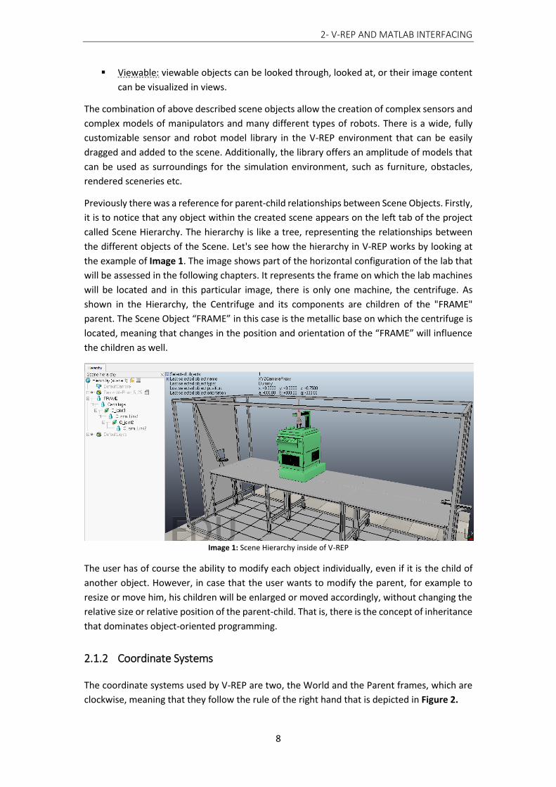
Previously there was a reference for parent-child relationships between Scene Objects. Firstly,
it is to notice that any object within the created scene appears on the left tab of the project
called Scene Hierarchy. The hierarchy is like a tree, representing the relationships between
the different objects of the Scene. Let's see how the hierarchy in V-REP works by looking at
the example of Image 1. The image shows part of the horizontal configuration of the lab that
will be assessed in the following chapters. It represents the frame on which the lab machines
will be located and in this particular image, there is only one machine, the centrifuge. As
shown in the Hierarchy, the Centrifuge and its components are children of the "FRAME"
parent. The Scene Object “FRAME” in this case is the metallic base on which the centrifuge is
located, meaning that changes in the position and orientation of the “FRAME” will influence
the children as well.
Image 1: Scene Hierarchy inside of V-REP
The user has of course the ability to modify each object individually, even if it is the child of
another object. However, in case that the user wants to modify the parent, for example to
resize or move him, his children will be enlarged or moved accordingly, without changing the
relative size or relative position of the parent-child. That is, there is the concept of inheritance
that dominates object-oriented programming.
2.1.2 Coordinate Systems
The coordinate systems used by V-REP are two, the World and the Parent frames, which are
clockwise, meaning that they follow the rule of the right hand that is depicted in Figure 2.

2- V-REP AND MATLAB INTERFACING
9
The world frame [x, y, z] = [0, 0, 0] position is its origin in V-REP. Any movement of an object
along the three axes is measured with respect to this point. If we wish to move an object at
the origin of the world frame, all of the position values with respect to the “World” should be
set to zero. In order to better monitor movements and rotations, the axes of the global
coordinate system (world frame) always appear in the lower right corner of the screen. Color
coding is set accordingly to R (Red), G (Green), B (Blue) X, Y, Z and is used to facilitate the
recognition of the axes.
The local coordinate system, referring to the parent, shows the position and rotation of an
object with respect to its parent's coordinate system respectively.
Figure 2: Clockwise coordinate system
If the user wishes to translate or rotate an object in the simulation scene, an additional option
is given, specifically the option to move the object with respect to its own frame, meaning
that the object does not take into consideration the position or orientation of the world frame
or of the parent frame of the object, but rather it is handled as a solo standing entity in the
simulation scene. To better understand the way that the local reference frame works, Image
2 and Image 3 are attached.
Image 2: Orientation of Parent_Frame with respect to the World Frame
In Image 2 the cylinder is child of the cube. Comparing the cube coordinate system
(Parent_Frame) with the global coordinate system of VREP, we observe a 90 ° rotation around
the Z axis, which is also written in the orientation window of the cube.

2- V-REP AND MATLAB INTERFACING
10
Looking now at the cylinder coordinate system (Child_Frame) in Image 3, we observe a
rotation of 180 ° around the Z axis of the global frame, but the orientation window shows a
rotation of 90 °. This is because the cylinder has rotated 90 ° with respect to its parent, but
has also adopted the rotation of the cube to the global system. Therefore, in its sum, the
rotation of the Child_Frame with respect to the World coordinate system equals 180o.
Image 3: Orientation of the Child_Frame with respect to its Parent Frame
2.1.3 3D Model Import and Neutral File Formats
Computer Aided Design (CAD) technology for engineering, and manufacturing is now playing
an increasingly important role in production industry. The importance of this technology to
increase productivity in engineering design has been widely recognized. These technologies
make it possible to shorten the time and lower the cost of development. Additionally, the
reliability and the quality of the product can be improved. CAD systems have therefore been
used in various fields of industry including automobile and aircraft manufacture, architecture
and shipbuilding, and there are currently many commercial systems available. SolidWorks,
Catia and Inventor are examples of available systems using CAD technology. With the
existence of a great diversity of CAD tools emerge the demand to import/export files between
different CAD software. The emergence of neutral format files and neutral format file
interfaces in order to exchange product data between CAD systems solve this problem. The
most widely accepted formats have been the Initial Graphics Exchange Standard (IGES), the
Standard d’Echange et de Transfert (SET), the STandard for the Exchange of Product model
data (STEP) and the Standard Transform Language (STL).[9]
The simulator V-REP does offer some basic geometrical shapes, as mentioned previously, that
can be used to model basic objects and structures. Yet, to model more difficult geometries,
these basic 3D Objects the software offers are not sufficient and are rather time consuming if
used for this case. V-REP therefore provides the ability to import 3D models from other design
programs. V-REP uses triangular meshes to describe and display shapes and for this reason it
only imports formats that describe objects as triangular meshes. If however importing objects

2- V-REP AND MATLAB INTERFACING
11
described as parametric surfaces for example (e.g. IGES, etc.) is desired, then first conversion
of the file to an appropriate triangular mesh format should be done.
V-REP supports following file-formats for shape import ([Menu bar --> File --> Import -->
Mesh...]):
OBJ: Wavefront Technologies file format. This is currently the only format that allows
importing of textured meshes in V-REP.
DXF: AutoCAD file format (Autodesk). Non-3D information that might be contained in
the file is ignored.
STL (ASCII or binary): 3D Systems file format. ASCII and binary files are supported.
COLLADA
URDF
2.2 Communication between MATLAB and the V-REP platform
Concerning the control of the behavior of the simulation objects, there is a wide range of
mechanisms used for this purpose, which characterize the V-REP framework that is
schematically presented in Figure 3. These controllers can be implemented not only inside of
the simulation environment, but also outside of it.
Figure 3: V-REP communication framework[10]
The main internal control mechanism is the use of child scripts, which can be associated with
any element in the scene. The child scripts handle a specific part of the simulation and they
are an integral part of their associated object. Due to that property they can be duplicated
and serialized, together with them. Therefore, they are a single package containing the model
parameters together with its control which makes them portable and scalable. Child scripts
have two execution modes. Non-threaded child scripts are pass-through scripts which means
every time they are called they execute some task and then return to control. Threaded child
scripts launch in thread and are handled by the main script code. The latter require more
advanced programming knowledge compared to non-threaded child scripts, while they take

2- V-REP AND MATLAB INTERFACING
12
up more processing power and time, causing lagging in response to simulation commands.
The main script handles both threaded and non-threaded child scripts. These embedded
scripts open and handle communication lines, start remote API servers, launch executables,
load and unload plugins.
V-REP also offers a method to control the simulation from outside the simulator by externally
applied controller algorithms. The remote API interface in V-REP communicates with the
simulation scene using socket communication. It is composed by remote API server services
and remote API clients. The client side can be developed in C/C++, Python, Java, Matlab or
other languages, also embedded in any software running on remote control hardware or real
robots, and it allows remote function calling, as well as fast and bidirectional data streaming.
Functions support two calling methods to adapt to any configuration: blocking, waiting until
the server replies, or non-blocking, reading streamed commands from a buffer.
On the client side, which is the application the user is running, at least 2 threads will be
running: the main thread -the one from which remote API functions are called-, and the
communication thread -the one that is handling data transfers behind the scenes. There can
be as many communication threads as needed on the client side. The server side, which is
implemented with a V-REP plugin, operates in a similar way. Figure 4Figure 4 illustrates the
remote API modus operandi.
Figure 4: Remote API functionality overview[10]
2.3 Enabling the remote API
To enable the remote API on the server side, in other words on V-REP's side, the remote API
plugin must be successfully loaded at V-REP start-up. The remote API plugin can start as many
server services as needed and each service will be listening/communicating on a different
port. A server service can be started in two different ways:
2- V-REP AND MATLAB INTERFACING
13
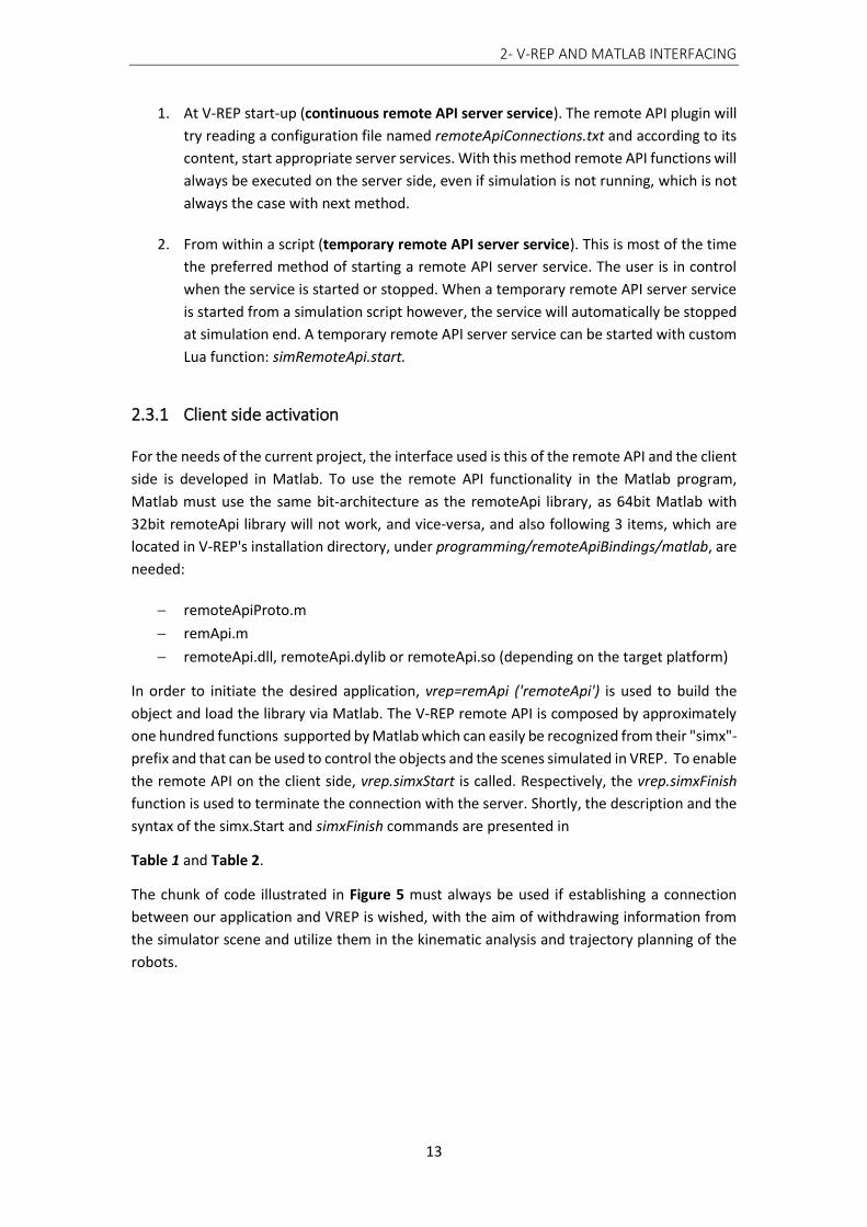
1. At V-REP start-up (continuous remote API server service). The remote API plugin will
try reading a configuration file named remoteApiConnections.txt and according to its
content, start appropriate server services. With this method remote API functions will
always be executed on the server side, even if simulation is not running, which is not
always the case with next method.
2. From within a script (temporary remote API server service). This is most of the time
the preferred method of starting a remote API server service. The user is in control
when the service is started or stopped. When a temporary remote API server service
is started from a simulation script however, the service will automatically be stopped
at simulation end. A temporary remote API server service can be started with custom
Lua function: simRemoteApi.start.
2.3.1 Client side activation
For the needs of the current project, the interface used is this of the remote API and the client
side is developed in Matlab. To use the remote API functionality in the Matlab program,
Matlab must use the same bit-architecture as the remoteApi library, as 64bit Matlab with
32bit remoteApi library will not work, and vice-versa, and also following 3 items, which are
located in V-REP's installation directory, under programming/remoteApiBindings/matlab, are
needed:
remoteApiProto.m
remApi.m
remoteApi.dll, remoteApi.dylib or remoteApi.so (depending on the target platform)
In order to initiate the desired application, vrep=remApi ('remoteApi') is used to build the
object and load the library via Matlab. The V-REP remote API is composed by approximately
one hundred functions supported by Matlab which can easily be recognized from their "simx"-
prefix and that can be used to control the objects and the scenes simulated in VREP. To enable
the remote API on the client side, vrep.simxStart is called. Respectively, the vrep.simxFinish
function is used to terminate the connection with the server. Shortly, the description and the
syntax of the simx.Start and simxFinish commands are presented in
Table 1 and Table 2.
The chunk of code illustrated in Figure 5 must always be used if establishing a connection
between our application and VREP is wished, with the aim of withdrawing information from
the simulator scene and utilize them in the kinematic analysis and trajectory planning of the
robots.

2- V-REP AND MATLAB INTERFACING
14
Figure 5: MATLAB code for establishing and terminating communication with V-REP platform
Table 1: Enabling the remote API-client side, Matlab documentation for simxStart function
simxStart
Description Starts a communication thread with the server (i.e. V-REP). A same client may
start several communication threads (but only one communication thread for a
given IP and port). This should be the very first remote API function called on the
client side. Make sure to start an appropriate remote API server service on the
server side that will wait for a connection. See also simxFinish. This is a remote
API helper function.
Matlab synopsis [number clientID]=simxStart(string connectionAddress,number
connectionPort,boolean waitUntilConnected,boolean
doNotReconnectOnceDisconnected,number timeOutInMs,number
commThreadCycleInMs)
Matlab parameters connectionAddress: the ip address where the server is located (i.e. V-REP)
connectionPort: the port number where to connect. Specify a negative port
number in order to use shared memory, instead of socket communication.
waitUntilConnected: if true, then the function blocks until connected (or timed
out).
doNotReconnectOnceDisconnected: if true, then the communication thread will
not attempt a second connection if a connection was lost.
timeOutInMs:
if positive: the connection time-out in milliseconds for the first connection
attempt. In that case, the time-out for blocking function calls is 5000
milliseconds.
if negative: its positive value is the time-out for blocking function calls. In that
case, the connection time-out for the first connection attempt is 5000
milliseconds.
commThreadCycleInMs: indicates how often data packets are sent back and
forth. Reducing this number improves responsiveness, and a default value of 5 is
recommended.
Matlab return
values
clientID: the client ID, or -1 if the connection to the server was not possible (i.e.
a timeout was reached). A call to simxStart should always be followed at the end
with a call to simxFinish if simxStart didn't return -1

2- V-REP AND MATLAB INTERFACING
15
Table 2: Enabling the remote API-client side, Matlab documentation for simxFinish function
2.3.2 Server side activation
To enable the remote API on the server side, utilized is the temporary remote API server
service, via the command simRemoteApi.start, which in our case is called from a non-threaded
child script attached to the Base Arm Link of the robotic arm, which is the parent of all links of
the robot. Shortly, the description and the syntax of the simRemoteApi.start command is
presented in Table 3 :
simRemoteApi.start
Description Starts a temporary remote API server service on the specified port. When
started from a simulation script, the service will automatically end when the
simulation finishes
Lua synopsis number result=simRemoteApi.start(number portNumber,number
maxPacketSize=1300,Boolean debug=false,Boolean preEnableTrigger=false)
Lua parameters
portNumber: port where to install the server service. Ports above 20000 are
preferred. Negative port numbers can be specified in order to use shared
memory, instead of socket communication.
maxPacketSize: the maximum size of a socket send-packet. Make sure to
keep the value at 1300, unless the client side has a different setting.
Debug: if true, a window will display the data traffic on that port.
preEnableTrigger: if true, the server service will be pre-enabled for
synchronous trigger signals from the client.
Lua return values
-1 if operation was not successful. In a future release, a more differentiated return value might be available
Table 3: Enabling the remote API –server side, LUA documentation for simRemoteApi.start function
The server side activation has following structure as shown in Figure 6, which was extracted from the VREP environment.
Figure 6: LUA code for server-side activation
simxFinish
Description Ends the communication thread. This should be the very last remote API function
called on the client side. simxFinish should only be called after a successfull call
to simxStart. This is a remote API helper function.
Matlab synopsis simxFinish(number clientID)
Matlab parameters
clientID: the client ID. refer to simxStart. Can be -1 to end all running
communication threads.
Matlab return values
None
2- V-REP AND MATLAB INTERFACING
16
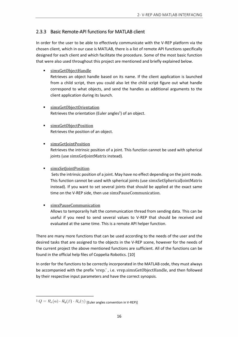
2.3.3 Basic Remote-API functions for MATLAB client
In order for the user to be able to effectively communicate with the V-REP platform via the
chosen client, which in our case is MATLAB, there is a list of remote API functions specifically
designed for each client and which facilitate the procedure. Some of the most basic function
that were also used throughout this project are mentioned and briefly explained below.
simxGetObjectHandle
Retrieves an object handle based on its name. If the client application is launched
from a child script, then you could also let the child script figure out what handle
correspond to what objects, and send the handles as additional arguments to the
client application during its launch.
simxGetObjectOrientation
Retrieves the orientation (Euler angles1) of an object.
simxGetObjectPosition
Retrieves the position of an object.
simxGetJointPosition
Retrieves the intrinsic position of a joint. This function cannot be used with spherical
joints (use simxGetJointMatrix instead).
simxSetJointPosition
Sets the intrinsic position of a joint. May have no effect depending on the joint mode.
This function cannot be used with spherical joints (use simxSetSphericalJointMatrix
instead). If you want to set several joints that should be applied at the exact same
time on the V-REP side, then use simxPauseCommunication.
simxPauseCommunication
Allows to temporarily halt the communication thread from sending data. This can be
useful if you need to send several values to V-REP that should be received and
evaluated at the same time. This is a remote API helper function.
There are many more functions that can be used according to the needs of the user and the
desired tasks that are assigned to the objects in the V-REP scene, however for the needs of
the current project the above mentioned functions are sufficient. All of the functions can be
found in the official help files of Coppelia Robotics. [10]
In order for the functions to be correctly incorporated in the MATLAB code, they must always
be accompanied with the prefix ‘vrep.’ , i.e. vrep.simxGetObjectHandle, and then followed
by their respective input parameters and have the correct synopsis.
1 [Euler angles convention in V-REP)]

3- THE ROBOTS
17
3 THE ROBOTS
3.1 The custom SCARA robot of Experoment
3.1.1 Description
SCARA robots were first developed in the 1980’s in Japan and the name SCARA stands for
Selective Compliance Assembly Robot Arm. The main feature of the SCARA robot is that it has
a jointed two-link arm which in some ways imitates the human arm, hence the often used
term articulated. It operates on a single plane, allowing the arm to extend into confined areas
and then retract or “fold up” out of the way, which makes it suitable for reaching inside
enclosures or pick-and-place from one location to another. [11]
The custom arm used in this study has 5 degrees of freedom, which depict the joints of the
robot. Of them, three (3) are revolute and two (2) prismatic joints. The arm is mounted on a
horizontal rail above the machines of the lab, for the needs of this study. The structure of the
SCARA robot studied in the current thesis is shown in Image 4.
Image 4: Structure of custom SCARA robot
Horizontal Base Joint
(prismatic)
Vertical Base Joint
(prismatic)
Arm Joint 1
(revolute)
Arm Joint 2
(revolute)
Arm Joint 3
(revolute)

3- THE ROBOTS
18
Each joint has its own stand-alone motor that allows it to move independently, within some
boundaries, which are shown in Table 4 and Table 5, and to move the second link between
every two that it connects. The robotic arm can be separated into two sections:
1. the translational joints (prismatic) movements of the robot vertically and
horizontally on the rails
2. the rotary joints (revolute) rotation of the robot to its vertical axis
Therefore, the limits of the two tables are expressed in different units, since in the 1st case we
are referring to translation, which equals meters, and in the 2nd case to rotation, which equals
degrees.
Table 4: Translational Joint Limits of the SCARA type robot
Table 5: Rotary Joint Limits of the SCARA type robot
The boundaries of the joints determine the working space of the arm that is defined as the
space that the end-effector can reach in any orientation. For the SCARA robot, the working
space is shown in Figure 7. In our case however, some restrictions apply as to the reach of
the workspace, since it has to be taken into consideration that the robot is hang from a rail,
which should not interfere with the movement of the arm. Therefore, the workspace for the
SCARA type robot used in the current thesis is smaller than the actual workspace, something
which is depicted in by the black line which represents the rail from which the arm is hung.
Translational Joints 1 2
Range(m) 3.7 1.9
Limits(m) -1.9, 1.8 0, 1.9
Rotary Joints 3 4 5
Range(O) 240 286 180
Limits(O) -120, 120 -143, 143 -90,90
Figure 7: Workspace of SCARA type robot

3- THE ROBOTS
19
3.1.2 Advantages and limitations of SCARA robots
The SCARA robot is most commonly used for pick-and-place or assembly operations where
high speed and high accuracy is required. Generally a SCARA robot can operate at higher
speed and with optional cleanroom specification. In terms of repeatability, currently available
SCARA robots can achieve tolerances lower than 10 microns, compared to 20 microns for a
six-axis robot. By design, the SCARA robot suits applications with a smaller field of operation
and where floor space is limited, the compact layout also making them more easily re-
allocated in temporary or remote applications.
On the other side, due to their configuration, the SCARA robots are typically only capable of
carrying a relatively light payload, typically up to 2 kg nominal (10 kg maximum). The envelope
of a SCARA robot is typically circular, which does not suit all applications, and the robot has
limited dexterity and flexibility compared to the full 3D capability of other types of robot. For
example, following a 3D contour is something that will be more likely fall within the
capabilities of a six-axis robot. [12]
3.2 Stäubli ΤX2-90XL
3.2.1 Description
The second robot used to run simulations of the experiments is the Stäubli TX2-90XL Robot.
The TX designation indicates a low payload, while the XL refers to the length of the arm. For
the purposes of the current study, the extra-long arm will be used. This arm is sufficiently
flexible and is able to perform a great variety of
applications, such as:
Handling of loads
Assembly, process, application of adhesive beads
Control check
Clean room applications
The arm consists of six links, which are connected in pairs of
two, by six rotary joints. The links of the robot are shown in
Figure 8 and are named accordingly and are each
represented with a capital letter. The links of the Stäubli
TX2-90XL are named after human body parts, because of its
anthropomorphic form.
Α – Base
B – Shoulder
C – Arm
D – Elbow
E – Forearm
F – Wrist Figure 8: Stäubli TX2-90XL Robot

3- THE ROBOTS
20
Movements on the arm joints are generated by servomotors coupled with position sensors.
Each of these motors is equipped with a parking break. The motors allow for each joint to
rotate independently, within some boundaries, which are shown in Table 6, and to move the
second link between every two that it connects. For example, joint 1 moves link B and joint 2
moves link C.
Table 6: Joint Limits of the Stäubli TX90XL
The boundaries of the joints determine the working space of the arm that is defined as the
space that the end-effector can reach in any orientation. For the Stäubli TX2-90XL, the
working space is shown in Figure 9.
The Stäubli robot has multiple mounting configurations (floor/wall/ceiling) to make its
integration into the production line easier. Figure 10 shows four different ways that the
Staubli TX2-90XL Robot can be mounted, while more information on the technical
specifications of the model can be found in Appendix B.
Joint Limits
Joint 1 2 3 4 5 6
Range(O) 360 277.5 280 540 255 540
Limits(O) ±180 -130, +147.5 ±145 ±270 -115, 140 ±270
Figure 9: Working space of Staubli TX2-90XL [Source: Staubli]

3- THE ROBOTS
21
Figure 10: Different mounting positions for Staubli TX2-90XL
3.2.2 Advantages and limitations of 6-axis robots
Articulated robots, or 6-axis robots, are easier to align to multiple planes, simple to operate
and maintain, and easily redeployed for automation applications and for a wide range of
upstream and downstream applications. They present high repeatability and accuracy, while
being able to reach orientations and positions, which are not possible by other robots. At the
same time however, they have greater demands as far as their working space and cost is
concerned.
3.3 Robot 3D Model Import
In the present work, the design of the Staubli robot was downloaded from the official CAD
Library of Staubli, whereas the design of the custom robotic arm was done in Autodesk's
AutoCAD and was received as ready file from the experoment team. The robot models were
exported in URDF, a file format mentioned in previous chapters, and then entered in the
simulation scene.
3- THE ROBOTS
22
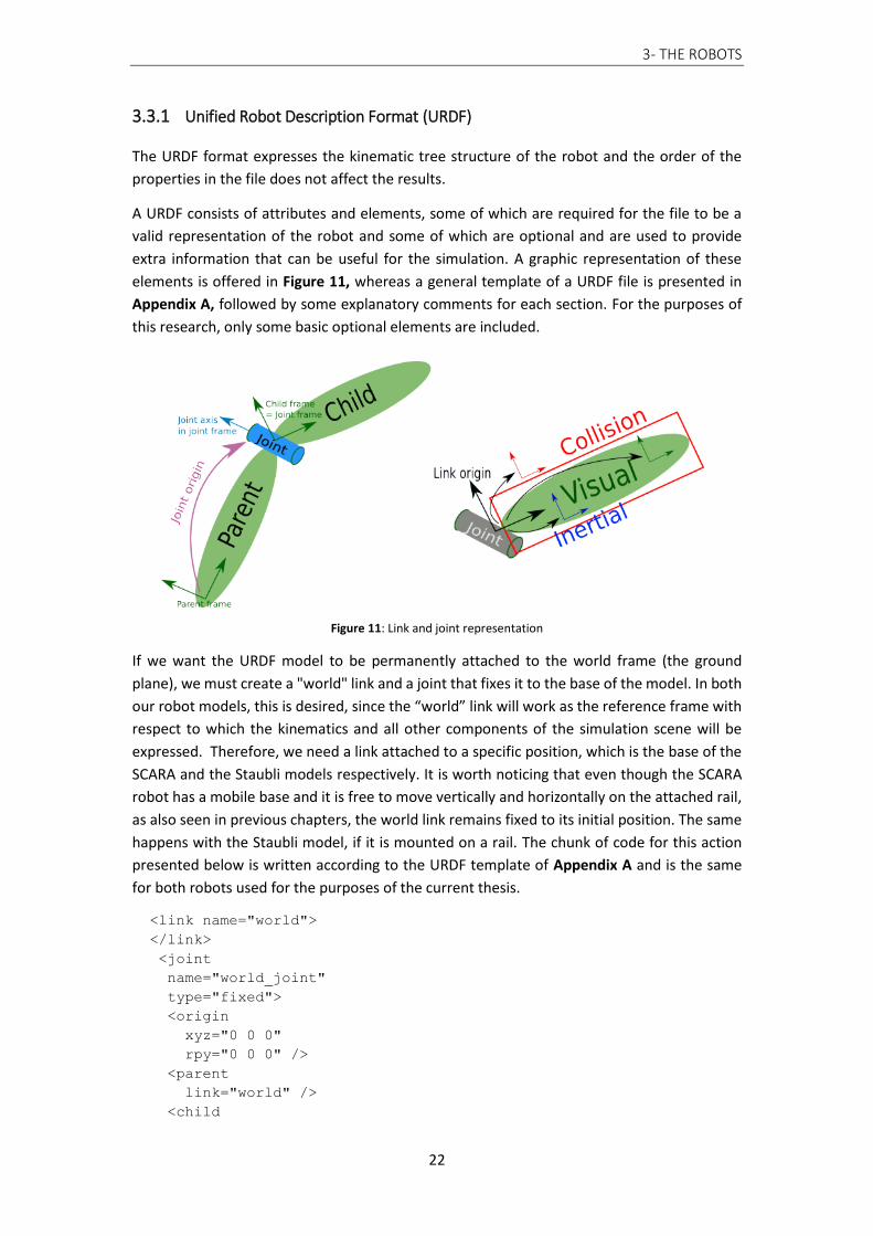
3.3.1 Unified Robot Description Format (URDF)
The URDF format expresses the kinematic tree structure of the robot and the order of the
properties in the file does not affect the results.
A URDF consists of attributes and elements, some of which are required for the file to be a
valid representation of the robot and some of which are optional and are used to provide
extra information that can be useful for the simulation. A graphic representation of these
elements is offered in Figure 11, whereas a general template of a URDF file is presented in
Appendix A, followed by some explanatory comments for each section. For the purposes of
this research, only some basic optional elements are included.
Figure 11: Link and joint representation
If we want the URDF model to be permanently attached to the world frame (the ground
plane), we must create a "world" link and a joint that fixes it to the base of the model. In both
our robot models, this is desired, since the “world” link will work as the reference frame with
respect to which the kinematics and all other components of the simulation scene will be
expressed. Therefore, we need a link attached to a specific position, which is the base of the
SCARA and the Staubli models respectively. It is worth noticing that even though the SCARA
robot has a mobile base and it is free to move vertically and horizontally on the attached rail,
as also seen in previous chapters, the world link remains fixed to its initial position. The same
happens with the Staubli model, if it is mounted on a rail. The chunk of code for this action
presented below is written according to the URDF template of Appendix A and is the same
for both robots used for the purposes of the current thesis.
<link name="world">
</link>
<joint
name="world_joint"
type="fixed">
<origin
xyz="0 0 0"
rpy="0 0 0" />
<parent
link="world" />
<child

3- THE ROBOTS
23
link="First_link_of_robot_model" />
</joint>
Respectively, an additional link is fixed to the last link of the robot model, representing the
end-effector frame that will be the part following the trajectory, which will be calculated in
the kinematics chapter. The origin attributes xyz and rpy depend on the position and
orientation of the parent link and are added in a way so that the ee_link is located
approximately at the edge of the parent link, which is usually the tool flange of the robot or
the edge of the gripper.
<link name="ee_link">
</link>
<joint
name="ee_joint"
type="fixed">
<origin
xyz="x y z"
rpy="r p y" />
<parent
link="Last_link_of_robot_model" />
<child
link="ee_link" />
</joint>
It is worth noting that in the case that the ee_link is located on the tool flange, a suitable offset to the actual gripping edge should be taken into consideration, since the position where the gripper is attached differs from the part which actually follows the trajectory and which is no other but the gripper fingers. Usually, a dummy is utilized in the simulation to represent the finger edge which will be grabbing the product, with respect to which the offset to the ee_link is set.
For every URDF file, its name is mentioned in the beginning with the name attribute:
<robot
name>
</robot>
and the file is saved with the same name as ‘name.urdf’.
3.3.2 Robot Coordinate Systems
For the expression of the position and the orientation of the links of a robotic arm, utilized are
usually the three (3) following coordinate systems. [13]
1. Global Coordinate System: A Cartesian coordinate system is located on the base of
the robot and all the positions of its distinct links are expressed with respect to this
frame.
2. Coordinates of End-Effector: The cartesian coordinate system is located on the edge
of the robotic arm, always taking it’s rotation into consideration.
3- THE ROBOTS
24
3. Joint Coordinate Frames: The position of each joint, for example the angle of a
rotational joint, is used for describing the position and configuration of the robot at
all times.
It is crucial that these coordinate frames are the same, in orientation and position, both in the
URDF file as well as in the VREP simulator. Otherwise, the results may diverge from the actual
positions and orientations that the robotic manipulators should acquire.
3.3.3 Scaling Factor
Upon importing the URDF file in the simulation environment, of the many options available,
one that is of interest and on which the accuracy of the research result depends is the Scale
Factor, which the user has to adjust in order to get realistic results. The question is now: why
is it so important to have realistic results rather than something nearly accurate?
The purpose of the current project is to virtually move the robots in the 3 dimensions of space
and to read the position and rotation of the end-effector point (EE) on the 3 axes. From these
6 numbers, the inverse kinematics (see Chapter 6) will result in the values of the angles of the
joints, which can then be loaded onto the real robot and set up a physical simulation. Since
the mathematics of the robot's kinematic chain depend on its physical dimensions, if the
dimensions of the simulation model are not exactly the same as those of the real robot, the
results will not only be inaccurate, but they may not correspond to the actual movement of
the robot at all. In our case, both robots and all machinery have been designed according to
their real dimensions and the transformation of the units from millimeters [mm] of the
SolidWorks and Creo files to meters [m] in VREP takes place automatically upon import.
Therefore, the scale factor of all components of the simulation scenes is 1. By setting different
values to the scale factor, the respective size is multiplied by the respective scaling factor.
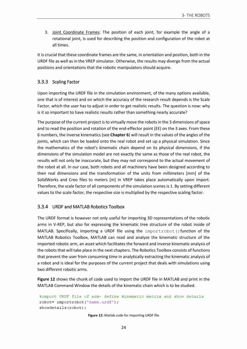
3.3.4 URDF and MATLAB Robotics Toolbox
The URDF format is however not only useful for importing 3D representations of the robotic
arms in V-REP, but also for expressing the kinematic tree structure of the robot inside of
MATLAB. Specifically, importing a URDF file using the importrobot()function of the
MATLAB Robotics Toolbox, MATLAB can read and analyze the kinematic structure of the
imported robotic arm, an asset which facilitates the forward and inverse kinematic analysis of
the robots that will take place in the next chapters. The Robotics Toolbox consists of functions
that prevent the user from consuming time in analytically extracting the kinematic analysis of
a robot and is ideal for the purposes of the current project that deals with simulations using
two different robotic arms.
Figure 12 shows the chunk of code used to import the URDF file in MATLAB and print in the
MATLAB Command Window the details of the kinematic chain which is to be studied.
Figure 12: Matlab code for importing URDF file
3- THE ROBOTS
25
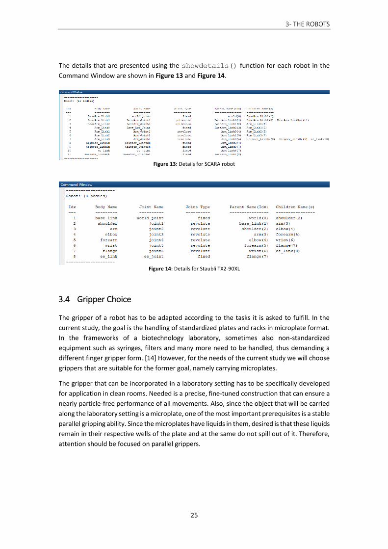
The details that are presented using the showdetails() function for each robot in the
Command Window are shown in Figure 13 and Figure 14.
Figure 13: Details for SCARA robot
Figure 14: Details for Staubli TX2-90XL
3.4 Gripper Choice
The gripper of a robot has to be adapted according to the tasks it is asked to fulfill. In the
current study, the goal is the handling of standardized plates and racks in microplate format.
In the frameworks of a biotechnology laboratory, sometimes also non-standardized
equipment such as syringes, filters and many more need to be handled, thus demanding a
different finger gripper form. [14] However, for the needs of the current study we will choose
grippers that are suitable for the former goal, namely carrying microplates.
The gripper that can be incorporated in a laboratory setting has to be specifically developed
for application in clean rooms. Needed is a precise, fine-tuned construction that can ensure a
nearly particle-free performance of all movements. Also, since the object that will be carried
along the laboratory setting is a microplate, one of the most important prerequisites is a stable
parallel gripping ability. Since the microplates have liquids in them, desired is that these liquids
remain in their respective wells of the plate and at the same do not spill out of it. Therefore,
attention should be focused on parallel grippers.

3- THE ROBOTS
26
Image 5: Example of parallel servo-gripper
[Source: Applied Robotics]
3.4.1 Parallel Grippers
A parallel gripper for handling multiwell plates in an automated analysis system, moves
individual multiwell plates between workstations, for example from a plate storage array unit
to an imaging station. More particularly, the gripper has two parallel plate-gripping arms that
move in equal, but opposite linear directions, and are controlled using a stepper motor. Each
of the arms has a shelf that provides support for the corresponding side edge of a multiwell
plate. [16]
1. SCARA
For the Scara type robot, the gripper choice is quite simple, since the robot itself
moves in a planar way, rotating only around the z axis. Therefore, a parallel gripper is
sure to maintain the desired orientation of the well plate – parallel to the lab floor-
and fulfill its task. Along with the 3D CAD models of the SCARA robot, incorporated is
a custom made parallel gripper, whose design drawing is provided in Appendix B. The
difference to common grippers is that it includes a rotating base for the fingers, an
addition that contributes to the change of orientation during loading or unloading the
well-plates, if necessary. For simplification purposes, the gripper in the simulation of
the SCARA remained as it is.
Alternatively, if the rotating base for the fingers is not deemed necessary, a good
alternative would be LGR Electric Servo Gripper “The Gripster”. More information on
the LGR Electric Servo Gripper can be found in Appendix B.
2. STAUBLI TX2-90XL
For the Stäubli model which is an articulated robot, the gripper choice is vast and can
be done in many different ways, always according to the needs of the respective
laboratory and the tasks at hand. Due to its 6-dof nature, the tool-flange can acquire
multiple different positions and orientations along and around the x, y and z axis. The
need for the microplate to remain parallel to the ground is vital in this case.

3- THE ROBOTS
27
For this robot model, the LGR Electric Servo Gripper can be a suitable solution, since
it can be easily mounted on the Stäubli and is fully compatible with the Stäubli model
series, while at the same time providing a stable parallel grip for the desired tasks.
PTM Präzitionstechnik also offers good alternatives to the gripper choice.
ROBOTIQ provides an alternative gripper solution. Though it is suitable for industrial
purposes and factory work, it can also be used inside a biotechnology laboratory and
be either vertically or horizontally located. More information can be found under
Appendix B.
This gripper choice was also used for the simulation purposes, since it was of the few
gripper designs that were provided online as 3D CAD models. Unfortunately, the CAD
files are for visual purposes only and are not thus functional, in the sense that the
gripping for the case of the Staubli model will not be simulated.
Image 6: ROBOTIQ 2F-140 Gripper[Source: ROBOTIQ]
The general idea, no matter the choice of company, remains the same. The objective is to
incorporate grippers that have a stroke of at least the greatest dimensions of the well-plates
that will be used. Smaller stroke grippers will not be able to grab the plate in both portrait and
landscape orientations, since they will not have an opening wide enough to clamp the
microplate.
The grippers that will be used for the simulations are thus:
The custom made gripper by experoment for the SCARA
The 2F-140 gripper by ROBOTIQ for the Staubli.

4- LABORATORY EQUIPMENT
28
4 LABORATORY EQUIPMENT
4.1 Machines
The machines that may be included in a Biotechnology Lab vary according to the experiments
that are to be conducted. Some demand few steps in order to be completed, however others
are extremely complicated and demand specific conditions and treatment, something that
equals the need for more specialized equipment in the lab. Therefore, there is no standard
when it comes to how many and which machines will be added in one lab, but it all depends
on the experimentation demands of the people running the laboratory and of course, the cost
margin that each company wants to abide by.
For the needs of the current project, included in the lab simulation, are following machines,
accompanied by their basic specifications. They are all compatible with automation solutions
so that they can be used in a robotic biotech lab. More on their dimensions and form can be
found in Appendix B.
4.1.1 Liquid Handler
Multipurpose liquid handling automated workstations are tools designed to do much of the
sampling, mixing, and combining of liquid samples automatically. Liquid handlers can measure
out samples, add reagents, and make sure liquids are added to bioassays in a uniform fashion.
The volume of sample the liquid handling automated workstation can handle is one feature
to consider when making a purchase. Other features to consider include how large a footprint
the workstation makes and the ease of use of its software interface. For our simulation, used
is the robotic Liquid Handler of Opentrons.
Rendered Visualization [Source:Opentrons ]
Specification (Biochem)
Specification (Mechanical / Automation)
Handles 96 & 384 standard well plates
Includes internal robotic arm to move plates between decks
Dispense range [0.5-250μL]
Has a hand-off position which is unobstructable and easily
accessible by external robotic arms
Cooling deck
Has the ability to be fed (by external robotic arm) pipette tips
Orbital shake deck
Has the ability to remove waste (by handing it off to the external
robotic arm)

4- LABORATORY EQUIPMENT
29
4.1.2 Centrifuge
A centrifuge is a laboratory device that is used for the separation of fluids, gas or liquid, based
on density. Separation is achieved by spinning a vessel containing material at high speed; the
centrifugal force pushes heavier materials to the outside of the vessel. This apparatus is found
in most laboratories from academic to clinical to research and used to purify cells, subcellular
organelles, viruses, proteins, and nucleic acids. There are multiple types of centrifuge, which
can be classified by intended use or by rotor design. In addition to its basic form presented
below, a robotic gripper can be mounted externally above the insertion opening for the plate,
so that the plate can be grabbed directly from the centrifuge. The latter will be the case for
the needs of the current project. For our simulation, used is ROTANTA 460 Robotic, a
centrifuge by Hettich.
Rendered Visualization [Source: Hettich]
Specification (Biochem)
Specification (Mechanical / Automation)
1000g max centrifugal force
Has the ability to be fed a well plate from the external
robotic arm
4.1.3 Freezer
Laboratory refrigerators are used to cool samples or specimens for preservation. They include refrigeration units for storing blood plasma and other blood products, as well as vaccines and other medical or pharmaceutical supplies. They differ from standard refrigerators used in homes or restaurant because they need to be totally hygienic and completely reliable. Laboratory refrigerators need to maintain a consistent temperature in order to minimize the risk of bacterial contamination and explosions of volatile materials. For our simulation, used is STR44, a freezer of Liconic.
Rendered Visualization [Source: Liconic]
Specification (Biochem)
Specification (Mechanical / Automation)
-20 oC
Has the ability to be fed a
well plate from the external robotic arm
~50 well plate capacity
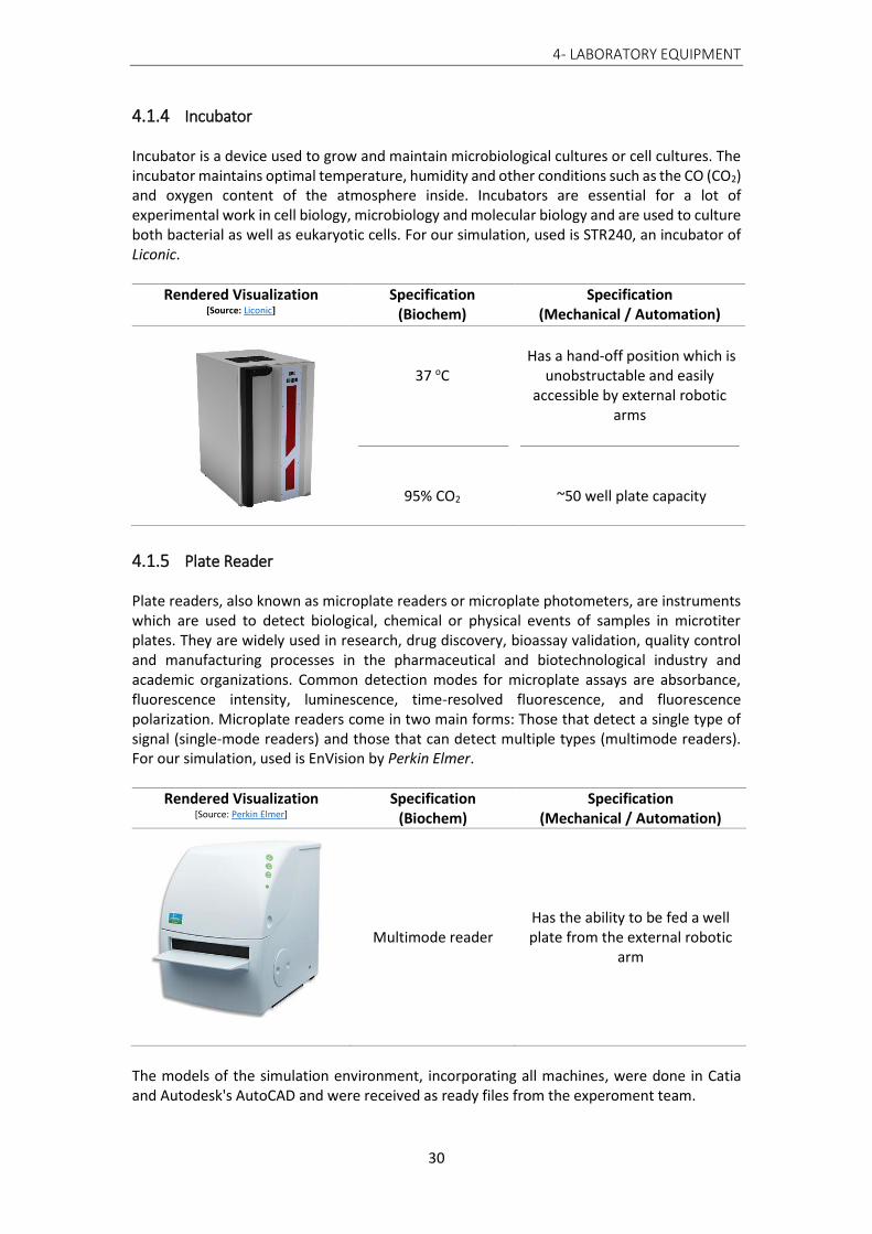
4- LABORATORY EQUIPMENT
30
4.1.4 Incubator
Incubator is a device used to grow and maintain microbiological cultures or cell cultures. The incubator maintains optimal temperature, humidity and other conditions such as the CO (CO2) and oxygen content of the atmosphere inside. Incubators are essential for a lot of experimental work in cell biology, microbiology and molecular biology and are used to culture both bacterial as well as eukaryotic cells. For our simulation, used is STR240, an incubator of Liconic.
Rendered Visualization [Source: Liconic]
Specification (Biochem)
Specification (Mechanical / Automation)
37 oC
95% CO2
Has a hand-off position which is
unobstructable and easily accessible by external robotic
arms
~50 well plate capacity
4.1.5 Plate Reader
Plate readers, also known as microplate readers or microplate photometers, are instruments which are used to detect biological, chemical or physical events of samples in microtiter plates. They are widely used in research, drug discovery, bioassay validation, quality control and manufacturing processes in the pharmaceutical and biotechnological industry and academic organizations. Common detection modes for microplate assays are absorbance, fluorescence intensity, luminescence, time-resolved fluorescence, and fluorescence polarization. Microplate readers come in two main forms: Those that detect a single type of signal (single-mode readers) and those that can detect multiple types (multimode readers). For our simulation, used is EnVision by Perkin Elmer.
Rendered Visualization [Source: Perkin Elmer]
Specification (Biochem)
Specification (Mechanical / Automation)
Multimode reader
Has the ability to be fed a well plate from the external robotic
arm
The models of the simulation environment, incorporating all machines, were done in Catia and Autodesk's AutoCAD and were received as ready files from the experoment team.

4- LABORATORY EQUIPMENT
31
4.2 Consumables
Sample reactions can be assayed in 1 - to -1536 well format microtiter plates. The most
common microplate format used in academic research laboratories or clinical diagnostic
laboratories is 96-well , which is an 8 x 12 matrix, with a typical reaction volume between 100
and 200 µL per well. Higher density microplates, with 384 (16 x 24 matrix) or 1536 wells, are
typically used for screening applications, when the number of samples processed per day, in
other words the throughput, and assay cost per sample become critical parameters, with a
typical assay volume between 5 and 50 µL per well. A 96- and 384- wellplate are presented in
Figure 14.
Irrespective of the number of wells, the dimensions of the microplates usually remain the
same, a fact that facilitates their handling by the robotic arm. The dimensions and drawings
of the microplates can be found in Appendix B, where basic elements of the well plates are
mentioned. In general, the well plates follow a specific standardization, therefore dimensions
remain the same among different production companies.
Figure 15: Cell-carrier 96 on the left and Cell-carrier 384 on the right

5- LABORATORY STRUCTURE AND LAYOUTS
32
5 LABORATORY STRUCTURE
AND LAYOUTS
5.1 Flexible Manufacturing Systems (FMS)
A flexible manufacturing system is a manufacturing system that contains enough flexibility to
allow the system to rapidly react to production changes. This flexibility is generally considered
to fall into two categories. The first is machine flexibility. This allows the system to be changed
to produce new product types and to change the order of operations executed on a part. The
second is routing flexibility. This consists of the ability to use multiple machines to perform
the same operation on a part as well as the system's ability to absorb large-scale changes,
such as in volume, capacity, or capability.[17]
Most FMS systems consist of three main systems: a material handling system to optimize the
flow of parts, a central control computer that controls material movement, and the working
machines, which are often automated machines or robots.
Control optimization, material flow efficiency, setup efficiency, and data flow efficiency can
be achieved by using Flexible Manufacturing Systems. Economical machining is achieved by:
Exploiting the flexibility and productivity of numerically controlled machine tools for
the production of smaller and medium sized lots
Utilizing costly production equipment more effectively through the reduction or
elimination of setups
Changing parts, tools, and machining programs automatically.[18]
5.2 Production line layouts for FMS
The analogies of FEPS to FMS are obvious and therefore layouts used for Flexible
Manufacturing can also be applied in the current project.
There are alternatives to setting up a robotic production cell for a biotechnology laboratory,
which vary according to the needs and the restrictions that apply each time. Some of these
needs and restrictions can be:
Limited working space, narrow aisles and floor obstructions
Number and position of machines in the cell

5- LABORATORY STRUCTURE AND LAYOUTS
33
Desired production rates and times
Flexibility in production for implementing low cost alternatives inside the cell
Aesthetics
Depending on these parameters, there is a range of different set-up alternatives to choose
from. Modelled and analyzed for the purposes of the thesis will be 3 of the most popular
layouts, namely:
1. Linear layout
2. Island (or Circular) layout
3. Ladder layout
5.2.1 Linear layout
The linear layout constitutes a very common production layout, which offers flexibility and
possibilities for extension. Specifically, scaling-up production is easier with this kind of format,
since increasing the number of machines in a cell, would mean elongation of the production
line to the wished extend, without any problem. The only restriction for its implementation
are the dimensions of the space available. This layout is ideal for narrow, but long spaces,
where a robot can be mounted on a rail and easily move along the lab space and to the
machines. For the needs of this layout, a SCARA type robot is sufficient, since the movements
of the robot are specific and restricted to planar movements in space. SCARA robots offer an
ergonomic alternative to more complex types of robots, in an economic as well as in a controls
respect.
However, as flexible as this layout can be, its implementation may result in unnecessary
motion between the workstations.[19] For example, if an experiment, in our case, consists of
a two-step procedure between two workstations that are each located on opposite sides, then
the translation times of the robot between the machines increases with the length of the
production line and results in unnecessary motion, since the whole production line has to be
run through, in order for only two machines to communicate.
A representation of this layout is presented in Figure 16.
5.2.2 Island (or Circular) Layout
The island layout, which could also be described as circular, involves the concept of a robot
centered cell, meaning that the machines are organized in a circular manner around the robot.
This format constitutes an effective layout when considering product movement as all the
Figure 16: Linear layout for production
Legend
Machine
Flow Path

5- LABORATORY STRUCTURE AND LAYOUTS
34
necessary operations to produce a component or subassembly are performed in close
proximity, resulting in near zero operation-to-operation transfer times.[19] At the same time,
this layout is suitable for limited space availability. In contrast to the linear layout, it also
facilitates access in the lab, since human interference might be deemed necessary at some
point.
On the other side of things, the islands are isolated with respect to each other, since the
formation is circular and does not allow communication between the robots, which are
located in the middle of each cell. This layout also offers finite possibilities of extension, a
factor that constricts flexibility since the number of additional machines that can be
incorporated in the cell is restricted. More specifically, the possible reaching area for the
robotic arm reaches a maximum, which cannot be overcome, no matter how much the
diameter of the cyclic layout is increased in order for more machines to be added. As for the
robot that can be used for this type of layout, recommended is a 6-DOF (Degrees Of Freedom)
robot to ensure maximum flexibility, since in this case wished is achieving any position and
orientation in the lab space. This equals increased cost and more complex robot control
strategies.
A representation of this layout is presented in
Figure 17.
Figure 17: Island (or circular) layout for production
5.2.3 Vertical Ladder Layout
The vertical ladder layout is a differentiation to the ladder layout implemented for horizontal
production cells. The machines in the vertical ladder layout are located in levels above each
other, creating a ladder formation, which resembles the design of library shelfs, each of which
is basically a different machine. This layout can be used in combination with either the linear
or island layouts in order to increase their extension possibilities, having the same advantages
and disadvantages as mentioned before in each case respectively.
The linear production can be thus extended in length and height, if the machines are organized
according to the ladder layout, by using a longer vertical rail that can help the robot reach
both the lowest and highest positions of the machines in the lab, always with respect to the
dimension restrictions of the lab space. Accordingly, the same is valid for the circular layout,
where no modifications are needed, since a 6-DOF can reach all the positions and orientations
in space that fall within its capabilities and working space.
A representation of this layout is presented in Figure 18.
Machine
Flow Path
Legend

5- LABORATORY STRUCTURE AND LAYOUTS
35
5.3 Laboratory Structure
Following the above mentioned guidelines, as far as production organization and layouts are
concerned, we can now create possible structures for the robotic biotechnology cloud lab
analyzed in this thesis, taking into consideration specific restrictions and facts concerning our
case and modelling demands. Some of these factors are analyzed below.
I. Available robotic arms
As already mentioned in previous chapters, we have two alternatives as to what kind
of robots will be used to simulate the experiment production flow. The one is the
custom SCARA robot provided by experoment and the second one the 6-DOF robotic
arm Staubi TX2-90XL.
SCARA: As mentioned previously, the SCARA robot is ideal, due to its smaller weight,
cost and easier control, when compared to a 6-DOF robot, for implementing a linear
layout in the production line. Therefore, mounting it on a vertical rail, which is then
connected to a horizontal rail hung on the lab wall, covering in that way translations
of the robot along the height and the length of the lab respectively, while organizing
the machines in a linear fashion.
STAUBLI: The Staubli can also be mounted in the same way from the ceiling of the lab,
covering a bigger work space than the SCARA, which in the case of the linear layout
does not actually offer any more benefits to the structure, since the movements are
very simple. Therefore, the Staubli in the linear layout increases the cost and
complexity of the system, without essentially increasing production flexibility. In the
contrary, the Staubli would be ideal for the island layout, reaching positions in space
that the SCARA cannot.
II. Available working space
The available lab space for the experoment team for now has following dimensions:
Length: 4,96 m | Width: 1,84 m | Height: 2,24 m
This equals a very narrow but long laboratory that restricts the possible layouts of the
lab to linear, since this is the only way for the machines and the robot to fit in this
space.
Flow Path
Machine
Legend
Figure 18: Vertical Ladder layout for production

5- LABORATORY STRUCTURE AND LAYOUTS
36
However, when considering scaling up a start-up, space should not be restrictive of
testing new configurations for future implementation and development. Therefore,
supposing that we want the lab to at least take up no more area in square meters [m2]
than the already available space, which equals 9,13 m2, and keep its height to 2,24 m,
we could utilize a space with following dimensions:
Length: 3,02 m | Width: 3,02 m | Height: 2,24 m
to set up an island layout, where the robot will be located in the middle of the lab and
the rest of the machines around it in a circular fashion.
III. Number and position of machines in the cell
For the needs of the current project the number of machines that will be used to
simulate the experiments is five (5) and includes all of the machines that were
thoroughly mentioned in Chapter 4. This number does not constitute a restrictive
parameter for any of the available layouts. However, an increase in the number of
machines should be dealt with thoroughly.
In the same manner, the position of the machines does not play a decisive role in
structuring the lab, because all of the machines are used in the different experiments
without a specific order, thus there is no optimal position for each of the machines.
IV. Desired production rates and times
The experiments conducted in the platform are very time-consuming in the sense that
each step of an experiment might have a duration between 2 and even 24 hours.
Therefore the translation times of the robot from workstation to workstation is not a
decisive factor in setting up the laboratory. In spite of that, in case of very long linear
production lines, this should be taken into consideration, since it could add up to
disproportionate translation times to average experiment completion times.
Taking all of these factors into consideration, we can now visualize the two most beneficial
possible layouts for our laboratory, which are no other than the:
Linear layout with the SCARA robot (Image 7, Image 8)
Island layout with the Staubli TX2-90XL (Image 9,Image 10,Image 11)
It is worth mentioning that in the frameworks of this project, the ladder layout will not be
analyzed, since the number of machines does not demand such formation and for the
purposes of this study the two other layouts are sufficient. In case of an increase in the number
of machines or due to other factors which may demand the ladder layout, it can be formed
through simple modifications, such as lengthening the vertical rail in the linear lineout and
adjusting the heights of the machines in the circular layout.

5- LABORATORY STRUCTURE AND LAYOUTS
37
Image 7: Front view of linear layout for biotechnology lab
Image 8: Top view of linear layout for biotechnology laboratory
Image 9: Front view of island layout for biotechnology laboratory

5- LABORATORY STRUCTURE AND LAYOUTS
38
Image 10: Top view of island layout for biotechnology laboratory with possible Input and Output Positions2
Image 11: Diagonal view of the island layout for biotechnology laboratory
2 The gray cube represents the frame of the lab, in other words its limits. We could think of it as a metallic structure, similar to the case with the linear layout.
Input Position Output Position

6- KINEMATIC ANALYSIS OF MANIPULATORS
39
6 KINEMATIC ANALYSIS
OF MANIPULATORS
6.1 Introduction
In this chapter, the most basic details about the kinematics of manipulators will be mentioned
and thorough calculations and relationship derivations will be omitted, since for the needs of
the current project and for modelling two different robotic structures, the Robotics System
Toolbox [17] of MATLAB was utilized to facilitate the procedure and prevent unnecessary long
and complex mathematical calculations. This toolbox provides many features that are useful
for the study and simulation of classic type robotic arm, for example things like kinematics,
dynamics and trajectory generation. The toolbox also provides functions for handling and
converting data types, such as vectors, as well as homogeneous and unit-quaternions, axis-
angle transformations that are necessary to represent the position and orientation
respectively in the 3 dimensions.
It is crucial however that there is a solid background and knowledge of the kinematic analysis
of a robotic manipulator, so that the functions offered by the Robotics System Toolbox can be
used correctly.
6.2 Kinematics
Kinematics is the science of motion that treats the subject without regard to the forces that
cause it. Within the science of kinematics, one studies the position, the velocity, the
acceleration, and all higher order derivatives of the position variables -with respect to time or
any other variable(s). Hence, the study of the kinematics of manipulators refers to all the
geometrical and time-based properties of the motion. The relationships between these
motions and the forces and torques that cause them constitute the problem of dynamics. [20]
In order to deal with the complex geometry of a manipulator, we affix frames to the links of
the mechanism, and then describe the relationships between these frames. The study of
manipulator kinematics involves, among other things, how the locations of these frames
change as the mechanism articulates.
The central topic of this chapter is a method to compute the position and orientation of the
manipulator's end-effector relative to the base of the manipulator as a function of the joint
variables. In order to fulfill this goal, there are two problems that need to be solved: the direct
or forward kinematics problem and the inverse kinematics problem.

6- KINEMATIC ANALYSIS OF MANIPULATORS
40
6.2.1 Forward Kinematics
A manipulator consists of a series of rigid bodies (links) connected by means of kinematic pairs
or joints. Joints can be essentially of two types: revolute and prismatic. Conventional
representations of the two types of joints are sketched in Figure 19. The whole structure forms
a kinematic chain. One end of the chain is constrained to a base. An end-effector (gripper,
tool) is connected to the other end allowing manipulation of objects in space. From a
topological viewpoint, the kinematic chain is termed open, when there is only one sequence
of links connecting the two ends of the chain. Alternatively, a manipulator contains a closed
kinematic chain, when a sequence of links forms a loop. The mechanical structure of a
manipulator is characterized by a number of degrees of freedom (DOFs) which uniquely
determine its posture. Each DOF is typically associated with a joint articulation and constitutes
a joint variable .The aim of forward, or else direct, kinematics is to compute the pose of the
end-effector as a function of the joint variables.
Figure 19: Conventional representations of joints[21]
Figure 20: Description of the position and orientation of the end-effector frame[21]
The pose of a body with respect to a reference frame is described by the position vector of
the origin and the unit vectors of a frame attached to the body. The transformation describing
the position of the end-effector relative to the base is obtained by simply concatenating
transformations between frames fixed in adjacent links of the chain. This leads to finding an
equivalent 4x4 homogeneous transformation matrix that relates the spatial displacement of
the end-effector coordinate frame to the base frame. Hence, with respect to a reference

6- KINEMATIC ANALYSIS OF MANIPULATORS
41
frame Ob–xbybzb, the direct kinematics function is expressed by the homogeneous 4x4
transformation matrix:
𝑇𝑒𝑏(𝑞) = [
𝑛𝑒𝑏(𝑞) 𝑠𝑒
𝑏(𝑞) 𝑎𝑒𝑏(𝑞) 𝑝𝑒
𝑏(𝑞)0 0 0 1
]
, where q is the (n×1) vector of joint variables, ne, se, ae are the unit vectors of a frame
attached to the end-effector, and pe is the position vector of the origin of such a frame with
respect to the origin of the base frame Ob–xbybzb (Figure 20). ne, se, ae and pe are a function
of q. The frame Ob–xbybzb is termed base frame. The frame attached to the end-effector is
termed end-effector frame and is conveniently chosen according to the particular task
geometry. If the end-effector is a gripper, the origin of the end-effector frame is located at the
centre of the gripper, the unit vector ae is chosen in the approach direction to the object, the
unit vector se is chosen normal to ae in the sliding plane of the jaws, and the unit vector ne is
chosen normal to the other two so that the frame (ne, se, ae) is right-handed. [21]
6.2.2 Joint Space and Operational Space
As described in the previous sections, the direct kinematics equation of a manipulator allows
the position and orientation of the end-effector frame to be expressed as a function of the
joint variables with respect to the base frame. If a task is to be specified for the end-effector,
it is necessary to assign the end-effector position and orientation, eventually as a function of
time (trajectory). This is quite easy for the position. On the other hand, specifying the
orientation through the unit vector triplet (ne, se, ae) is quite difficult, since their nine
components must be guaranteed to satisfy the orthonormality constraints imposed before at
each time instant. This problem will be resumed in the Differential Kinematics section.
The problem of describing end-effector orientation admits a natural solution if one of the
above minimal representations is adopted. In this case, indeed, a motion trajectory can be
assigned to the set of angles chosen to represent orientation. Therefore, the position can be
given by a minimal number of coordinates with regard to the geometry of the structure, and
the orientation can be specified in terms of a minimal representation (Euler angles) describing
the rotation of the end-effector frame with respect to the base frame. In this way, it is possible
to describe the end-effector pose by means of the (m×1) vector, with m ≤ n,
𝑥𝑒 = [𝑝𝑒
𝜑𝑒]
, where 𝑝𝑒 describes the end-effector position and 𝜑𝑒 its orientation.
This representation of position and orientation allows the description of an end-effector task
in terms of a number of inherently independent parameters. The vector xe is defined in the
space in which the manipulator task is specified. Hence, this space is typically
called operational space. On the other hand, the joint space (configuration space) denotes the
space in which the (n×1) vector of joint variables
𝑞 = [
𝑞1
⋮𝑞𝑛
]

6- KINEMATIC ANALYSIS OF MANIPULATORS
42
, is defined. It is qi = ϑi for a revolute joint and qi = di for a prismatic joint. Accounting
for dependence of position and orientation from the joint variables, the direct kinematics
equation can be written in following form:
xe = k(q)
The (m×1) vector function k(·)— nonlinear in general — allows computation of the
operational space variables from the knowledge of the joint space variables. It is worth
noticing that the dependence of the orientation components of the function k(q) on the joint
variables is not easy to express except for simple cases. In fact, in the most general case of a
six-dimensional operational space (m = 6), the computation of the three components of the
function φe(q) cannot be performed in closed form but goes through the computation of the
elements of the rotation matrix, i.e., ne (q), se (q), ae (q). The equations that allow the
determination of the Euler angles from the triplet of unit vectors ne, se, ae were given before.
[21]
6.2.3 Inverse Kinematics
The direct kinematics establish the functional relationship between the joint variables and the
end-effector position and orientation. The inverse kinematics problem consists of the
determination of the joint variables corresponding to a given end-effector position and
orientation. The solution to this problem is of fundamental importance in order to transform
the motion specifications, assigned to the end-effector in the operational space, into the
corresponding joint space motions that allow execution of the desired motion.
As regards the direct kinematics equation with the transformation matrixes, the end-effector
position and rotation matrix are computed in a unique manner, once the joint variables are
known. On the other hand, the inverse kinematics problem is much more complex for the
following reasons:
The equations to solve are in general nonlinear, and thus it is not always possible to
find a closed-form solution
Multiple solutions may exist.
Infinite solutions may exist, e.g., in the case of a kinematically redundant manipulator.
There might be n admissible solutions, in view of the manipulator kinematic
structure. The existence of solutions is guaranteed only if the given end-effector
position and orientation belong to the manipulator dexterous workspace.
The existence of mechanical joint limits may eventually reduce the number of admissible
multiple solutions for the real structure. In cases where solutions do exist, they often cannot
be presented in closed form, so numerical methods are required. [21]
6.3 Differential Kinematics
In the previous section, direct and inverse kinematics equations establishing the relationship
between the joint variables and the end-effector pose were derived. In this section,
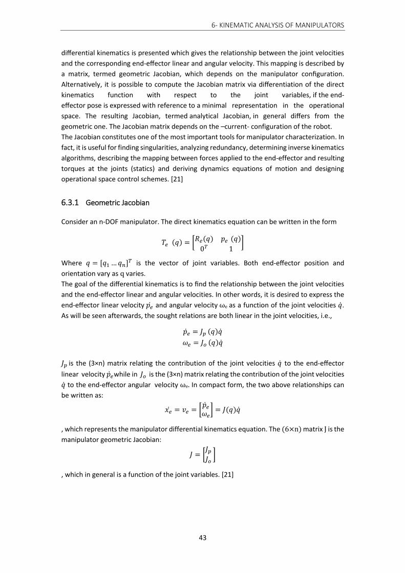
6- KINEMATIC ANALYSIS OF MANIPULATORS
43
differential kinematics is presented which gives the relationship between the joint velocities
and the corresponding end-effector linear and angular velocity. This mapping is described by
a matrix, termed geometric Jacobian, which depends on the manipulator configuration.
Alternatively, it is possible to compute the Jacobian matrix via differentiation of the direct
kinematics function with respect to the joint variables, if the end-
effector pose is expressed with reference to a minimal representation in the operational
space. The resulting Jacobian, termed analytical Jacobian, in general differs from the
geometric one. The Jacobian matrix depends on the –current- configuration of the robot.
The Jacobian constitutes one of the most important tools for manipulator characterization. In
fact, it is useful for finding singularities, analyzing redundancy, determining inverse kinematics
algorithms, describing the mapping between forces applied to the end-effector and resulting
torques at the joints (statics) and deriving dynamics equations of motion and designing
operational space control schemes. [21]
6.3.1 Geometric Jacobian
Consider an n-DOF manipulator. The direct kinematics equation can be written in the form
𝑇𝑒 (𝑞) = [𝑅𝑒(𝑞) 𝑝𝑒 (𝑞)
0𝑇 1]
Where 𝑞 = [𝑞1 … 𝑞𝑛]𝑇 is the vector of joint variables. Both end-effector position and
orientation vary as q varies.
The goal of the differential kinematics is to find the relationship between the joint velocities
and the end-effector linear and angular velocities. In other words, it is desired to express the
end-effector linear velocity 𝑝�̇� and angular velocity ωe as a function of the joint velocities �̇�.
As will be seen afterwards, the sought relations are both linear in the joint velocities, i.e.,
�̇�𝑒 = 𝐽𝑝 (𝑞)�̇�
𝜔𝑒 = 𝐽𝜊 (𝑞)�̇�
𝐽𝑝 is the (3×n) matrix relating the contribution of the joint velocities �̇� to the end-effector
linear velocity �̇�𝑒while in 𝐽𝜊 is the (3×n) matrix relating the contribution of the joint velocities
�̇� to the end-effector angular velocity ωe. In compact form, the two above relationships can
be written as:
𝑥�̇� = 𝑣𝑒 = [�̇�𝑒
𝜔𝑒] = 𝐽(𝑞)�̇�
, which represents the manipulator differential kinematics equation. The (6×n) matrix J is the
manipulator geometric Jacobian:
𝐽 = [𝐽𝑝
𝐽𝜊 ]
, which in general is a function of the joint variables. [21]

6- KINEMATIC ANALYSIS OF MANIPULATORS
44
6.3.2 Inverse Differential Kinematics
Previously, it was shown how the inverse kinematics problem admits closed-form solutions
only for manipulators having a simple kinematic structure. Problems arise whenever the end-
effector attains a particular position and/or orientation in the operational space, or the
structure is complex and it is not possible to relate the end-effector pose to different sets of
joint variables, or else the manipulator is redundant. These limitations are caused by the
highly non-linear relationship between joint space variables and operational space variables.
On the other hand, the differential kinematics equation represents a linear mapping between
the joint velocity space and the operational velocity space, although it varies with the current
configuration. This fact suggests the possibility to utilize the differential kinematics equations
to tackle the inverse kinematics problem. Suppose that a motion trajectory is assigned to the
end-effector in terms of ve and the initial conditions on position and orientation. The aim is
to determine a feasible joint trajectory (q(t), �̇�(t)) that reproduces the given trajectory. By
considering the relationship found above:
𝑣𝑒 = 𝐽(𝑞)�̇�
, the joint velocities can be obtained via simple inversion of the Jacobian matrix
𝑞 ̇ = 𝐽−1(𝑞)𝑣𝑒
If the initial manipulator posture q(0) is known, joint positions can be computed by
integrating velocities over time, i.e.
𝑞(𝑡) = ∫ 𝑞(𝜍)𝑑𝜍 ̇𝑡
0
+ 𝑞(0).
The integration can be performed in discrete time by resorting to numerical techniques. The
simplest technique is based on the Euler integration method, which is that given an
integration interval ∆t, if the joint positions and velocities at time tk are known, the joint
positions at time tk+1= tk+ Δt can be computed as
𝑞(𝑡𝑘 + 1) = 𝑞(𝑡𝑘) + �̇�(𝑡𝑘)𝛥𝑡
This technique for inverting kinematics is independent of the solvability of the kinematic
structure. Nonetheless, it is necessary that the Jacobian be square and of full rank .[21]
6.3.3 Kinematic Singularities
Kinematic singularities have long been recognized as causing one of the most serious
problems in programming and control of robotic manipulators. It is well-known that when a
manipulator is at-or is in the neighborhood of-a singular configuration, severe restrictions may
occur on its motion. Avoiding or reducing the effects of singularities has been an attractive
topic which has captured the attention of many researchers in robotics during the last decade.
A remarkable number of methods and/or algorithms aimed at computing well-behaved or
robust inverse kinematics solutions have been proposed in the literature, and many papers in
the past have presented simulation results. Close to a kinematic singularity, the usual inverse
differential kinematics solutions based on Jacobian (pseudo-) inverse become ill-conditioned,

6- KINEMATIC ANALYSIS OF MANIPULATORS
45
and this is experienced in the form of very high joint velocities and large control deviations.
Nonetheless, when a pre-programmed reference end-effector trajectory is to be tracked, it is
possible either to interpolate in joint coordinates close to singular configurations or to plan
motions so that singularities are avoided. On the other hand, in real-time and sensory control
of robotic manipulators, the reference trajectory is not known a priori and some remedies
must be taken in order to counteract the unexpected occurrence of singularities. The same
kind of problem is encountered in joy-stick control of a robot if the operator attempts to lead
the robot through-or nearby-a singularity using end-effector motion increments.[22]
6.4 Inverse Kinematics Algorithms
Computation of joint velocities is obtained by using the inverse of the Jacobian evaluated with
the joint variables at the previous instant of time
𝑞(𝑡𝑘 + 1) = 𝑞(𝑡𝑘) + 𝐽−1(𝑞(𝑡𝑘))𝑣𝑒(𝑡𝑘)𝛥𝑡
It follows that the computed joint velocities �̇� do not coincide with those satisfying
𝑞 ̇ = 𝐽−1(𝑞)𝑣𝑒
in the continuous time. Therefore, reconstruction of joint variables q is entrusted to a
numerical integration. As a consequence, the end-effector pose corresponding to the
computed joint variables differs from the desired one. This inconvenience can be overcome
by resorting to a solution scheme that accounts for the error between the desired and the
actual end-effector position and orientation. Let
𝑒 = 𝑥𝑑 − 𝑥𝑒
be the expression of such error.
Considering its derivative, we get:
�̇� = 𝑥�̇� − 𝑥�̇� = 𝑥�̇� − 𝐽(𝑞)�̇�
For this equation to lead to an inverse kinematics algorithm, it is worth relating the computed
joint velocity vector �̇� to the error e so that a differential equation describing error evolution
over time can be given. Nonetheless, it is necessary to choose a relationship between �̇� and e
that ensures convergence of the error to zero.
6.4.1 Inverse Jacobian
The inversion of the Jacobian, which was mentioned before, can represent a serious
inconvenience not only at a singularity but also in the neighborhood of a singularity. For
instance, for the Jacobian inverse it is well known that its computation requires the
computation of the determinant. In the neighborhood of a singularity, the determinant takes
on a relatively small value which can cause large joint velocities. [21]

6- KINEMATIC ANALYSIS OF MANIPULATORS
46
6.4.2 Pseudo-Inverse Jacobian
For kinematically redundant robots, the Jacobian matrix is non-square and its inverse can be
obtained using a pseudo-inverse 𝐽+. Specifically, if the Jacobian matrix J has a size of m rows
and n columns (m ≠ n), i.e., J is a non-square matrix, its inverse matrix cannot be computed.
In order to solve inverse kinematics task for this case, pseudoinverse of Jacobian matrix is
used, which is expressed as:
𝐽+ = (𝐽𝑇𝐽)−1 𝐽𝑇
Pseudoinverse J+, also called Moore-Penrose inverse of Jacobian matrix, gives the best
possible solution in the sense of least squares.
However, by using the pseudoinverse, the problems of singularities in the Jacobian still
remain. These singularities might occur for instance, when multiple links become aligned in
the same direction and subsequently, identical derivatives for several joints of the robot arm
are obtained. Inversion of nearly singular matrices results in excessively large velocities and
causes unrealistic behavior with oscillations around a singular configuration. In addition to
that, the limits of the robots are not taken into consideration and may lead to false and
inaccurate results.[23]
6.4.3 Damped Least Squares (DLS)
An effective strategy that allows motion control of manipulators in the neighborhood of
kinematic singularities is the damped least-squares technique, which is also the method that
was used within this study. The method corresponds to solving the equation:
𝐽𝑇(𝑞) �̇�𝑟 = (𝐽𝑇(𝑞) 𝐽(𝑞) + 𝜆2𝛪) �̇�
λ ≥ 0 is the damping factor and Ι is the (n x n) identity matrix, which depends on the
dimensions of the Jacobian and thus on the DOF of the respective robot. Also,
�̇�𝑟 = �̇�𝑑 + 𝐾𝑒
is the reference value vector with �̇�𝑑 that is the time derivative of the desired task function,
K is a positive definite(usually diagonal) matrix and e is the task-space error, to which the
orientation error can also be incorporated .[24]
It can be easily shown that the equation above can be formally written as
�̇� = (𝐽𝑇(𝑞)𝐽(𝑞) + 𝜆2𝛪)−1 𝐽𝑇(𝑞)�̇�𝑟
It is worth noting that when λ= 0, the damped least-squares solution reduces to a regular
matrix inversion which is ill-conditioned close to a singularity. So, it is essential to select
suitable values for the damping factor. Small values of λ give accurate solutions, but low
robustness to the occurrence of singular and near-singular configurations. Large values of λ
result in low tracking accuracy even when a feasible and accurate solution would be possible.
The damping factor λ determines the degree of approximation introduced with respect to the
pure least-squares solution. In the same manner, using a constant value for λ may turn out to

6- KINEMATIC ANALYSIS OF MANIPULATORS
47
be inadequate for obtaining good performance over the entire manipulator workspace. An
effective choice is to adjust λ as a function of some measure of closeness to the singularity at
the current configuration of the manipulator. Τo this purpose manipulability measures or
estimates of the smallest singular value can be adopted. A singular region can be defined on
the basis of the estimate of the smallest singular value of J. Outside the region the exact
solution is used, while inside the region a configuration varying damping factor is introduced
to obtain the desired approximate solution. The factor must be chosen so that continuity of
joint velocity q is ensured in the transition at the border of the singular region. We have
selected the damping factor according to the following law:
𝜆2 = {0
(1 − (𝜎
𝜀)2𝜆𝑚𝑎𝑥
2 , 𝜎 ≥ 𝜀
, 𝑜𝑡ℎ𝑒𝑟𝑤𝑖𝑠𝑒 }
, where σ : the estimate of the smallest singular value of J
ε : a threshold that defines the size of the singular region
The value of λmax is at the user's disposal to suitably shape the solution in the neighborhood
of a singularity. Utilizing the singular value decomposition method, we can find an estimate
of the smallest singular value of J. [22]
6.5 Trajectory Planning
The goal of trajectory planning is to generate the reference inputs to the motion control
system which ensures that the manipulator executes the planned trajectories. The user
typically specifies a number of parameters to describe the desired trajectory. Planning consists
of generating a time sequence of the values attained by an interpolating function, typically a
polynomial, of the desired trajectory.
The minimal requirement for a manipulator is the capability to move from an initial posture
to a final assigned posture. The transition should be characterized by motion laws requiring
the actuators to exert joint generalized forces which do not violate the saturation limits and
do not excite the typically modelled resonant modes of the structure. It is then necessary to
devise planning algorithms that generate suitably smooth trajectories. In order to avoid
confusion between terms often used as synonyms, the difference between a path and a
trajectory is to be explained. A path denotes the locus of points in the joint space, or in the
operational space, which the manipulator has to follow in the execution of the assigned
motion; a path is then a pure geometric description of motion. On the other hand, a trajectory
is a path on which a timing law is specified, for instance in terms of velocities and/or
accelerations at each point.
In principle, it can be conceived that the inputs to a trajectory planning algorithm are the path
description, the path constraints, and the constraints imposed by manipulator dynamics,
whereas the outputs are the end-effector trajectories in terms of a time sequence of the
values attained by position, velocity and acceleration. [21]
Whenever it is desired that the end-effector motion follows a geometrically specified path in
the operational space, it is necessary to plan trajectory execution directly in the same space.
Planning can be done either by interpolating a sequence of prescribed path points or by
generating the analytical motion primitive and the relative trajectory in a punctual way. In
6- KINEMATIC ANALYSIS OF MANIPULATORS
48
both cases, the time sequence of the values attained by the operational space variables is
utilized in real time to obtain the corresponding sequence of values of the joint space
variables, via an inverse kinematics algorithm.
To that respect, it is convenient to refer to the parametric description of paths in space. Then
let 𝑝 be a (3×1) vector and 𝑓 (𝜎) a continuous vector function defined in the interval [𝜎𝑖, 𝜎𝑓 ].
Consider the equation
𝑝 = 𝑓(𝜎)
With reference to its geometric description, the sequence of values of p with σ varying in
[𝜎𝑖, 𝜎𝑓 ] is termed path in space. The equation above defines the parametric representation
of the path Γ and the scalar σ is called parameter. As σ increases, the point p moves on the
path in a given direction. This direction is said to be the direction induced on Γ by the
parametric representation 𝑝 = 𝑓(𝜎). A path is closed when 𝑝(𝜎𝑓 ) = 𝑝(𝜎𝑖 ), otherwise it is
open.
Let 𝑝𝑖 be a point on the open path Γ on which a direction has been fixed. The arc length s of
the generic point p is the length of the arc of Γ with extremes p and pi if p follows pi, the
opposite of this length if p precedes pi. The point pi is said to be the origin of the arc length (s
= 0). From the above presentation it follows that to each value of s a well-determined path
point corresponds, and then the arc length can be used as a parameter in a different
parametric representation of the path Γ
𝑝 = 𝑓(𝑠) , 𝑠 ∈ [0,1]
, where 𝑠 =𝜎
𝐿, 𝜎 ∈ [0, 𝐿], with L representing the current length of the path.
The range of variation of the parameter s will be the sequence of arc lengths associated with
the points of Γ. Consider a path Γ represented by the relationship 𝑝 = 𝑓(𝑠). Let p be a point
corresponding to the arc length s. Except for special cases, p allows the definition of three unit
vectors characterizing the path. The orientation of such vectors depends exclusively on the
path geometry, while their direction depends also on the direction induced on the path. [21]
Considering the simplest case, which is connection of the initial and final points of a path with
line segments, the parametric representation of the path is expressed as following:
𝑝(𝑠) = 𝑝𝑖 + 𝑠 (𝑝𝑓 − 𝑝𝑖 )
The velocity of point 𝑝 is given by the time derivative of 𝑝:
�̇�(𝑠) = 𝑑𝑝
𝑑𝑠�̇� = (𝑝𝑓 − 𝑝𝑖) �̇�
Then, �̇� represents the magnitude of the velocity vector relative to point p, taken with the
positive or negative sign depending on the direction of �̇� along t. The magnitude of �̇� starts
from zero at t = 0, then it varies with a parabolic profile as the above choice of linear segments
for s(t), and finally it returns to zero at 𝑡 = 𝑡𝑓 .
Let 𝑥𝑒 be the vector of operational space variables expressing the pose of the manipulator’s
end-effector. Generating a trajectory in the operational space means to determine a function
𝑥𝑒(𝑡) taking the end-effector frame from the initial to the final pose in a time 𝑡𝑓 along a given
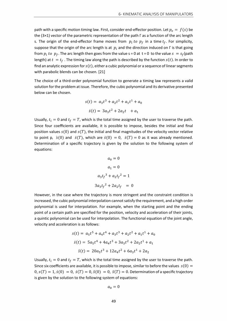
6- KINEMATIC ANALYSIS OF MANIPULATORS
49
path with a specific motion timing law. First, consider end-effector position. Let 𝑝𝑒 = 𝑓(𝑠) be
the (3×1) vector of the parametric representation of the path Γ as a function of the arc length
s. The origin of the end-effector frame moves from 𝑝𝑖 𝑡𝑜 𝑝𝑓 in a time 𝑡𝑓. For simplicity,
suppose that the origin of the arc length is at 𝑝𝑖 and the direction induced on Γ is that going
from 𝑝𝑖 𝑡𝑜 𝑝𝑓. The arc length then goes from the value s = 0 at t = 0 to the value 𝑠 = 𝑠𝑓(path
length) at 𝑡 = 𝑡𝑓 . The timing law along the path is described by the function 𝑠(𝑡). In order to
find an analytic expression for 𝑠(𝑡), either a cubic polynomial or a sequence of linear segments
with parabolic blends can be chosen. [21]
The choice of a third-order polynomial function to generate a timing law represents a valid
solution for the problem at issue. Therefore, the cubic polynomial and its derivative presented
below can be chosen.
𝑠(𝑡) = 𝑎3𝑡3 + 𝑎2𝑡2 + 𝑎1𝑡1 + 𝑎0
�̇�(𝑡) = 3𝑎3𝑡2 + 2𝑎2𝑡 + 𝑎1
Usually, 𝑡𝑖 = 0 and 𝑡𝑓 = 𝑇, which is the total time assigned by the user to traverse the path.
Since four coefficients are available, it is possible to impose, besides the initial and final
position values 𝑠(0) and 𝑠(𝑇), the initial and final magnitudes of the velocity vector relative
to point p, �̇�(0) and �̇�(𝑇), which are �̇�(0) = 0, �̇�(𝑇) = 0 as it was already mentioned.
Determination of a specific trajectory is given by the solution to the following system of
equations:
𝑎0 = 0
𝑎1 = 0
𝑎3𝑡𝑓3 + 𝑎2𝑡𝑓
2 = 1
3𝑎3𝑡𝑓2 + 2𝑎2𝑡𝑓 = 0
However, in the case where the trajectory is more stringent and the constraint condition is
increased, the cubic polynomial interpolation cannot satisfy the requirement, and a high order
polynomial is used for interpolation. For example, when the starting point and the ending
point of a certain path are specified for the position, velocity and acceleration of their joints,
a quintic polynomial can be used for interpolation. The functional equation of the joint angle,
velocity and acceleration is as follows:
𝑠(𝑡) = 𝑎5𝑡5 + 𝑎4𝑡4 + 𝑎3𝑡3 + 𝑎2𝑡2 + 𝑎1𝑡1 + 𝑎0
�̇�(𝑡) = 5𝑎5𝑡4 + 4𝑎4𝑡3 + 3𝑎3𝑡2 + 2𝑎2𝑡1 + 𝑎1
�̈�(𝑡) = 20𝑎5𝑡3 + 12𝑎4𝑡2 + 6𝑎3𝑡1 + 2𝑎2
Usually, 𝑡𝑖 = 0 and 𝑡𝑓 = 𝑇, which is the total time assigned by the user to traverse the path.
Since six coefficients are available, it is possible to impose, similar to before the values 𝑠(0) =
0, 𝑠(𝑇) = 1, �̇�(0) = 0, �̇�(𝑇) = 0, �̈�(0) = 0, �̈�(𝑇) = 0. Determination of a specific trajectory
is given by the solution to the following system of equations:
𝑎0 = 0
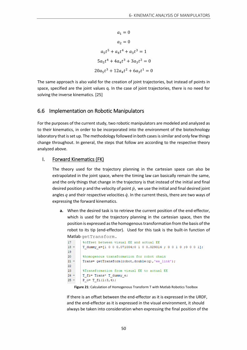
6- KINEMATIC ANALYSIS OF MANIPULATORS
50
𝑎1 = 0
𝑎2 = 0
𝑎5𝑡5 + 𝑎4𝑡4 + 𝑎3𝑡3 = 1
5𝑎5𝑡4 + 4𝑎4𝑡3 + 3𝑎3𝑡2 = 0
20𝑎5𝑡3 + 12𝑎4𝑡2 + 6𝑎3𝑡1 = 0
The same approach is also valid for the creation of joint trajectories, but instead of points in
space, specified are the joint values q. In the case of joint trajectories, there is no need for
solving the inverse kinematics. [25]
6.6 Implementation on Robotic Manipulators
For the purposes of the current study, two robotic manipulators are modeled and analyzed as
to their kinematics, in order to be incorporated into the environment of the biotechnology
laboratory that is set up. The methodology followed in both cases is similar and only few things
change throughout. In general, the steps that follow are according to the respective theory
analyzed above.
I. Forward Kinematics (FK)
The theory used for the trajectory planning in the cartesian space can also be
extrapolated in the joint space, where the timing law can basically remain the same,
and the only things that change in the trajectory is that instead of the initial and final
desired position 𝑝 and the velocity of point �̇�, we use the initial and final desired joint
angles 𝑞 and their respective velocities �̇�. In the current thesis, there are two ways of
expressing the forward kinematics.
a. When the desired task is to retrieve the current position of the end-effector,
which is used for the trajectory planning in the cartesian space, then the
position is expressed as the homogenous transformation from the basis of the
robot to its tip (end-effector). Used for this task is the built-in function of
Matlab getTransform.
Figure 21: Calculation of Homogenous Transform T with Matlab Robotics Toolbox
If there is an offset between the end-effector as it is expressed in the URDF,
and the end-effector as it is expressed in the visual environment, it should
always be taken into consideration when expressing the final position of the

6- KINEMATIC ANALYSIS OF MANIPULATORS
51
end-effector. For example, this offset could be presented when a new
gripper part is tested on a robot.
b. When the desired task is to bring the robot arm to a specific configuration and
when the position of the end-effector is of no importance, then the forward
kinematics are expressed with the help of the trajectory planning in the joint
space. For example, if we want the robot to always return to a fixed “Home”
configuration, then by setting the final configuration as 𝑞_𝑓 to specific values
for each joint, and by retrieving the current configuration 𝑞_𝑖 of the robot, the
trajectory can be planned. In this case there is no need for inverse kinematics
to be solved, since the final position of the end-effector does not play a
significant role. 𝑞_𝑓 and 𝑞_𝑓 are vectors of length (5x1) for the SCARA and
(6x1) for the STAUBLI. It is also possible to create separate programs that each
controls only a specific number of joints each time, if that is desired.
II. Trajectory Planning
For the trajectory planning, the simplest approaches possible have been adopted for
each separate case. Namely:
a. SCARA
Taking into account the structure of the SCARA type robot, which allows
movements along the x,y and z axis, however rotation only around one axis-
in our case the z axis-, the form of the trajectory does not need to be more
complicated than movements along linear segments. To that respect, the
cubic polynomial is used for the time law. The SCARA robot therefore
translates from one position to the next, following a straight line. The
intermediate points must thus be carefully selected, so as to abide by this
convention and receive better simulation results.
b. STAUBLI
As for the Staubli, which is a 6-axis robot, the trajectory is more stringent and
the constraints are increased. In that case the cubic polynomial interpolation
cannot satisfy the requirements, and a fifth order polynomial is used for
interpolation. The quantic polynomial ensures smoother transition between
the different positions when compared to the cubic polynomial and is
preferred for articulated robots, like the STAUBLI.
III. Jacobian
The Jacobian depends on the current configuration of the robot, it therefore changes
every time, since the orientation and position of the end-effector change accordingly.
In order to facilitate its calculation at every time step, the built-in function of Matlab
geometricJacobian is used. However, the Jacobian calculated by Matlab has
its rows reversed. Therefore, it is necessary to reverse their order before proceeding
further. The Jacobian retrieves the position and orientation of the end-effector to the
base frame of the robot.

6- KINEMATIC ANALYSIS OF MANIPULATORS
52
Figure 22: Calculation of Geometric Jacobian with Matlab Robotics Toolbox
a. SCARA: Only the three first and the last one rows are useful in the case of the
Jacobian for the SCARA type robot. This is due to the fact that SCARA robots
can only rotate around one axis, which in our case is the z-axis. Therefore, we
do not need the whole Jacobian matrix.
b. STAUBLI: The Staubli on the other hand, as a 6-axis robot, can move, as well
as rotate around all of the axis. Therefore, the whole Jacobian matrix is
maintained.
IV. Damping factor λ
The damping factor that is used for the DLS algorithm is calculated according to the
respective theory. SVD is utilized to retrieve the singular configuration matrix of the
Jacobian and to find in that way an estimate of the smallest singular value. 𝜆max was
chosen to equal 0.04 in our case. This value depends on the user and the robot at
hand. This number in our case was retrieved based on the robot models and the
bibliography recommendations. The threshold 𝜀 was calculated for the singular case
where the robot arms had all of their links aligned, which is a singular position for both
of the robots.
Figure 23: Calculation of damping factor λ with SVD
V. DLS
As mentioned before, the inverse kinematics algorithm that is used is expressed in the
equation below, which calculates the joint velocities of the robot.
�̇� = (𝐽𝑇(𝑞)𝐽(𝑞) + 𝜆2𝛪)−1 𝐽𝑇(𝑞)(𝑣𝑑 + 𝐾𝑒) (𝐼)
Incorporating the joint limits that apply in reality for a robotic manipulator can be
tricky. In order to include the limits that may already be specified for the robot, we
must reformulate the problem using quadratic programming.
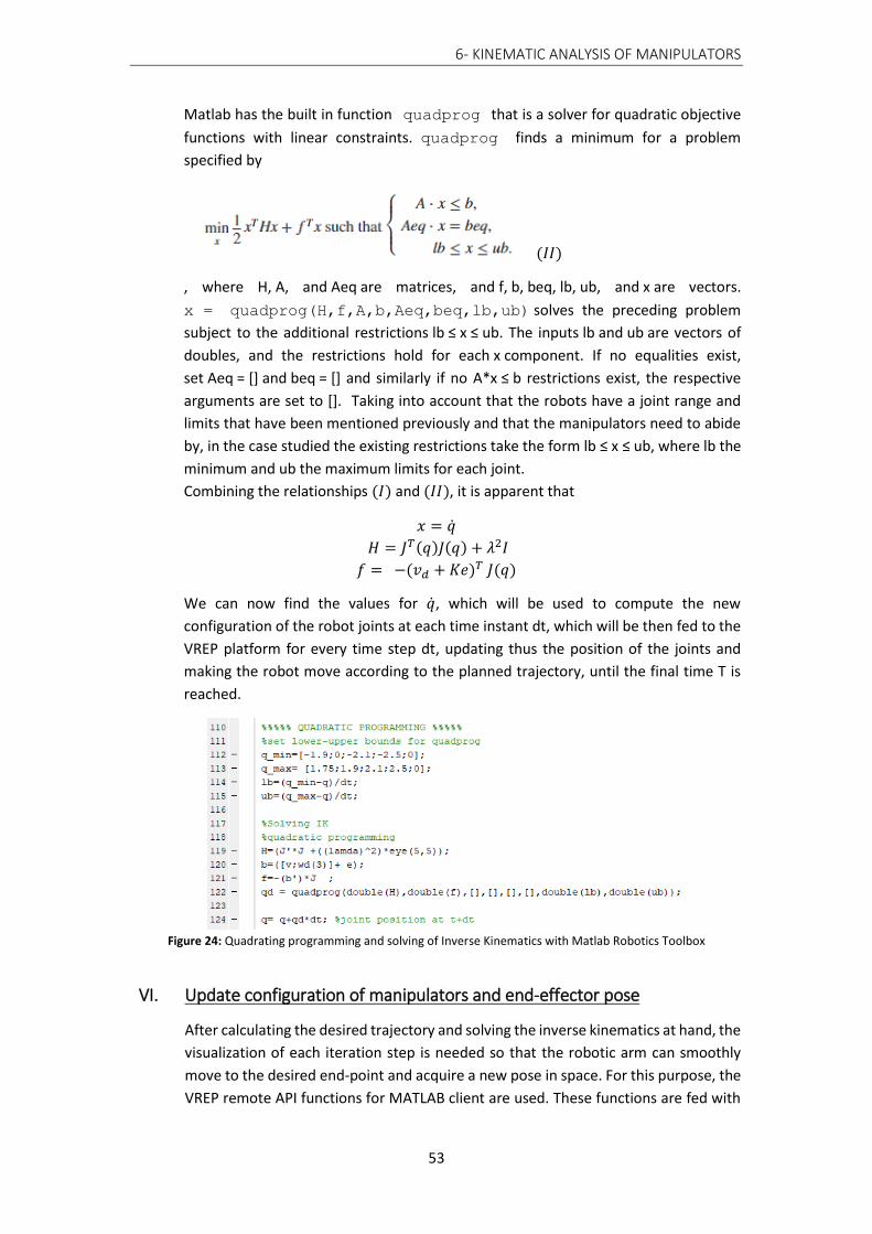
6- KINEMATIC ANALYSIS OF MANIPULATORS
53
Matlab has the built in function quadprog that is a solver for quadratic objective
functions with linear constraints. quadprog finds a minimum for a problem
specified by
(𝐼𝐼)
, where H, A, and Aeq are matrices, and f, b, beq, lb, ub, and x are vectors.
x = quadprog(H,f,A,b,Aeq,beq,lb,ub) solves the preceding problem
subject to the additional restrictions lb ≤ x ≤ ub. The inputs lb and ub are vectors of
doubles, and the restrictions hold for each x component. If no equalities exist,
set Aeq = [] and beq = [] and similarly if no A*x ≤ b restrictions exist, the respective
arguments are set to []. Taking into account that the robots have a joint range and
limits that have been mentioned previously and that the manipulators need to abide
by, in the case studied the existing restrictions take the form lb ≤ x ≤ ub, where lb the
minimum and ub the maximum limits for each joint.
Combining the relationships (𝐼) and (𝐼𝐼), it is apparent that
𝑥 = �̇�
𝐻 = 𝐽𝑇(𝑞)𝐽(𝑞) + 𝜆2𝛪
𝑓 = −(𝑣𝑑 + 𝐾𝑒)𝑇 𝐽(𝑞)
We can now find the values for �̇�, which will be used to compute the new
configuration of the robot joints at each time instant dt, which will be then fed to the
VREP platform for every time step dt, updating thus the position of the joints and
making the robot move according to the planned trajectory, until the final time T is
reached.
Figure 24: Quadrating programming and solving of Inverse Kinematics with Matlab Robotics Toolbox
VI. Update configuration of manipulators and end-effector pose
After calculating the desired trajectory and solving the inverse kinematics at hand, the
visualization of each iteration step is needed so that the robotic arm can smoothly
move to the desired end-point and acquire a new pose in space. For this purpose, the
VREP remote API functions for MATLAB client are used. These functions are fed with

6- KINEMATIC ANALYSIS OF MANIPULATORS
54
the new values of q that are calculated at each time step dt and are translated into
commands in the VREP environment, where the robot moves accordingly. The smaller
the time step dt is, the smoother and more accurate the final motion of the
manipulators is. This procedure from the beginning of the kinematic analysis to the
final visualization is shown in Figure 25.
Figure 25: Validation flowchart of kinematic model[26]
The robotic manager architecture, incorporating sensors and cameras for the live localization
of the machinery, the robotic arms and the well-plates is presented in Figure 26 schematically
for comprehension.
Figure 26: Robotic manager architecture
It is thus easily understood that the above mentioned approach, which is applied on two
different robotic manipulators, can also be applied on other various robotic arms with small
adjustments that mainly concern the robot itself, such as the number of DOF’s, the range and
limits of its joints as well as the lab settings that the robot is found in. However, it should be
noted that this methodology is followed for the case where the machinery has predefined
positions in space and also the consumables have predefined shapes and sizes. The behavior
of the system under different circumstances is unknown and will not be analyzed within the
frameworks of the current thesis.
INPUT

7- SIMULATION
55
7 SIMULATION
7.1 Visual Simulation Models
According to the information provided in the previous chapters, the simulation models that
will be tested can be finalized. The most important factor of the simulation that has been
stressed throughout the current project is to provide flexibility to the researcher and to be
parameterized in a way that any experiment protocol can be brought through, regardless of
the number or type of machines, the order of their use during an experiment or even
regardless of the background of the user.
7.1.1 Robots
After expressing the kinematic chain of each robot as URDF file the models are inserted in the
simulation scene. Each robot consists of its own links and joints, while in the URDF files two
more entities were added, namely the ee_link and the world, which were mentioned
in the respective chapter, as well.
The role of the world entity, which will be referred to as the robot’s world frame and is by
no means to be confused with the global frame of VREP, is to provide a reference frame for
everything that happens in the simulation scene. Since the robotic arms constitute the central
theme for the function of the robotic systems at hand, it is logical that not only the position
and orientation of the robotic links, but also the position and orientation of all the
components of a scene are expressed with reference to this frame. The world entity is fixed
in the laboratory space, which is mandatory to have uniformity in the expression of different
objects in the lab.
Respectively, the ee_link represents the actual final end-effector position, which is always
approximately the middle of the gripper and the point where the microplate is attached.
However, it is possible that the ee_link of the URDF file does not represent the actual gripping
point, but rather the base of the gripper or the final joint of a robot. In that case, a visual
ee_link_dummy is added in the VREP scene. The visual gripping point ee_link_dummy is then
expressed with respect to the ee_link of the URDF, via the respective offset and this is later
expressed with respect to the world. Maintaining a homogenous expression of position and
orientation is the key to a successful and accurate simulation.

7- SIMULATION
56
Image 12: ee_link_dummy for SCARA (left) and STAUBLI (right) robots
7.1.2 Lab Equipment
The lab equipment, including the machines, the input and output positions from which the
microplates are received and returned to at the beginning and the end of each experiment
respectively, as well as the consumables, are inserted in the scene according to the desired
layout. The goal is to create an environment, where the robot will be able to spot the loading
and unloading points of each machine with respect to the its world frame. In order for the
robot to understand, which machines it should visit during an experiment, dummy objects are
set in the loading-unloading positions of each machine and are named after their machines.
It is important that the orientation of these dummy points is the same as the orientation of
the ee_link_dummy so that the robotic arm may be able to approach the right position with
the correct orientation. Τhe positions where the robotic arms should unload and load a
microplate in the machines and the surroundings of the lab are presented in Image 13.
Image 13: Loading- unloading points of laboratory machines

7- SIMULATION
57
7.1.3 Safe Positions
These dummies are not only used to express the position and orientation of an object with
respect to the world frame of the robot, but are also used as references to describe some
other positions in space, which are necessary for the robot in order to plan its trajectory
smoothly.
For example it is highly recommended that intermediate points are used between the robot
Home position and any Machine Position. Defining a Machine Safe Position helps eliminate
collisions of the robot with the lab equipment. Such a machine position can be defined as the
(Machine Position +/- an offset). The offset can represent a distance from the actual loading-
unloading position which is deemed safe for the robot to approach, before completing its task.
Safe Positions in the experiments to follow are defined for following cases:
Before the SCARA robotic arm approaches the rotary base on which the microplates
change orientation to avoid collision with the machines during folding/ unfolding of
the arm and with itself
Before the SCARA robotic arm approaches the Input/ Output positions to avoid
collisions with the frame of the laboratory
Before the SCARA and the STAUBLI robotic arms approach the Loading/ Unloading
positions of each machine to avoid irregular arm movements and collisions with the
machines
In real-life experiments, this procedure is accomplished with the use of a live localization
system, which gives feedback to the robot as to its end-effector position with the use of
cameras and vision sensors.
7.1.4 Parameterization of the simulation
In our case, once the simulation environment is set and the dummies are defined, VREP stores
this information and communicates it to Matlab. So, for example, by giving a command to
Matlab for the robot to reach the Centrifuge, VREP having the machine’s position and
orientation stored, may parse this information to Matlab, where the code is responsible for
the rest. Therefore, parameterizing the problem at hand is easy.
The existence of multiple intermediate points makes it necessary for the trajectory to be
recalculated every time between two different points. More specifically, the trajectory is
computed every time that the robot needs to move between two points A and B. Matlab
requests from VREP the position and orientation of point A, which is the initial current position
P_o of the end-effector, as well as the position and orientation of point B, which is the final
desired position P_f the end-effector has to reach. After the robots moves from A to B, then
the new position A’ is basically the position B of the previous trajectory. In order for the robot
to start a new movement between A’ and C, a new trajectory with the updated positions has
to be recalculated. The trajectory is then followed by the robotic manipulator according to its
inverse kinematics programming and the position of the end-effector is updated in VREP at
every time step dt .

7- SIMULATION
58
Among other parameters that can be controlled by the user is the resolution of the results
and the smoothness of the robot’s movements. It is apparent that the smaller the time step
dt is, the more accurate and smooth the movement of the robot will be, since the
interpolation number is higher and more points of the trajectory are calculated.
7.2 Experiment Protocols
An experiment protocol describes the necessary actions for an experiment to be conducted,
from its beginning to its end. Examples of experimental protocols are provided below for two
experiments, which are dependent on each other, since Experiment 02 needs material from
Experiment 01.
Figure 27: Experiment protocol examples
KEY

7- SIMULATION
59
7.3 User Interface ( UI )
The facilitation of the communication between the user (researcher) and the simulation
environment is of major importance, since the platform must be accessible enough to people,
who do not have deep robotics knowledge. The goal is to simply communicate an experiment
protocol as presented above, with the least effort possible, thus building a UI friendly to its
user is the first step towards a successful simulation.
Upon starting the programs main_SCARA.m and main_STAUBLI.m, which are the two
Matlab programs responsible for everything that happens inside each lab, the user is asked to
Input working station:
At this point, the user can input the name of the workstations – laboratory machines – which
are included in the experiment and in the order that the user wishes each machine to be used,
along with the time that the user wishes for the test specimen to remain in each machine. The
available machine options that the user can type for the laboratories at hand are:
Opentrons
Centrifuge
EnVision
STR44
STR240
Each machine can be used more than once, if the experiment demands that a specific
workstation is visited multiple times. After including all the machines and respective times in
the correct order the user can type stop to indicate that the experiment protocol is complete
and that all the necessary equipment have already been referred to.
For the needs of the current study, the times have not been taken into consideration, since
they can even reach two days of waiting in a specific machine. Thus, this procedure is
represented by pausing the arm movements for a few seconds.
After the protocol is input in the platform, the program checks if the robot is located in its
Home position , which is a safe position for the robot to start any experiment. If it is, the user
is prompted with the notification:
Robot is in Home Position-Ready to start experiment
Otherwise, the robot moves to its Home position and then the user is asked for one last if
he/she wishes to proceed with the experiment. The default answer is set to YES.
Do you wish to continue to experiment? Y/N [Y]:
If the user types N, then the experiment is interrupted. If the user types Y, the experiment
starts according to its protocol.
After completion of the experiment, the user is notified accordingly:
Experiment successfully completed!

7- SIMULATION
60
Below, a flowchart is provided, representing the interaction of the user with the platform.
Figure 28: User interface flowchart
7.4 Simulation of Experiment with SCARA and STAUBLI
After the start of the experiment, the robot acquires different positions and configurations in
space, which depend on its final destination and the constraints that are imposed. Below, a
series of images is presented, showing a series of changes in the position and orientation of
the robotic arm for both the SCARA and the STAUBLI.
7.4.1 SCARA
Image 14: Home position of SCARA robot (input position) Image 15: SCARA grabbing plate from technician

7- SIMULATION
61
Image 17: Safe distance from machines for SCARA
Image 19: SCARA returning plate to technician (output
position)
Image 20: Return of SCARA to Home
Image 16: SCARA above well-plate on rotating base (used to change plate orientation if needed)
Image 18: Gripper is open ready to leave/grab plate
for SCARA

7- SIMULATION
62
7.4.2 STAUBLI TX2-90XL
Image 21: Home position of STAUBLI Image 22: STAUBLI grabbing plate from technician
Image 23 : Safe distance from machine for STAUBLI
Image 24: STAUBLI ready to leave/grab plate from machine

7- SIMULATION
63
Image 25: STAUBLI returning plate to technician
Image 26: Return of STAUBLI to Home

7- SIMULATION
64
7.5 Collision Detection
Collisions of the robotic arm with the surrounding area can cause significant damage both to
the robot itself and to the work being done. In the virtual environment, unlike the real one,
conflicts have no consequence and their purpose is to warn the user. In this way, the operator
can program the arm's trajectory, preventing collisions before they can occur.
V-REP can detect collisions between two collidable entities in a very flexible way. The
calculation is an exact interference calculation. The collision detection module will only detect
collisions, it does however not directly react to them, something which depends on the
dynamic modeling of the scene that exceeds the purposes of this thesis.
More specifically, a colliding property, also mentioned before, was added to both the robots
and all objects in the surrounding environment. This option helps recognize the collision
between two objects, while allowing for overlap. The collision detection module allows
registering collision objects which are collidable entity-pairs consisting of a collider entity and
collidee entity. During simulation, the collision state of each registered collision object can
then be visualized with a different coloring.
In order to define the collidable entity-pairs that we want to be detected during simulation,
utilized is the “collection” function of provided by VREP, which is a user-defined collection
of scene objects. V-REP supports calculations based not only on objects, but also on
collections. For instance the collision detection module allows registering following collision
pair: (collection A; object B). The collision checking algorithm will then check whether the
collection A (any object composing it) collides with object B. In our case we set three different
collections which refer respectively to:
COLLECTION A: All objects of which a robotic arm consists (chain, tip included)
COLLECTION B: The “body” of the robotic arms.
COLLECTION C: The rest of the components of the robotic arms (including tip and gripper).
The goal is to check for collisions between the robots and the surrounding objects of the scene
(COLLECTION A; All other entities-machines, frame, objects in scene) and to check for
collisions between the robotic arms and their “bodies”, since it is possible that a robot may
collide with itself as well. (COLLECTION B; COLLECTION C). When the two objects, between
which the collision is checked, stop contacting each other, the color of the entities is reset to
its initial state. The following pictures show some cases of robot collisions with other objects.

7- SIMULATION
65
Image 27: Collision of SCARA with rotating base Image 28: Collision of SCARA robot with Centrifuge
Image 29: Collision of SCARA robot with laboratory frame
Image 30: Collision of STAUBLI robot with Liquid Handler Image 31: Collision of STAUBLI robot with base
8- RESULTS
66
8 RESULTS 8.1 General Remarks
Following diagrams are the results of the simulations during different experiments. Only the
most basic movements of each robot are included in these diagrams for the sake of brevity,
however the behaviors of the robots do not change dramatically between movements. It is
important to note and pay attention to the scale of the axis of each diagram. Specifically, in
some cases the graphs may seem to diverge or present important errors, but this is usually
due to the scale of the axis whose magnitude might represent changes to the 10-3 .
For the SCARA it is worth noting that the 5th joint, namely the joint of the gripper, which
rotates it, is set to 0 for all the simulations at hand. This is due to the fact that since the
machines are all in a row there is no need for the gripper to rotate. If that is needed, then the
respective joint can be “activated” by setting its upper and lower limits in the
SCARAplatetraj.m program.
The same approach can also be utilized for the STAUBLI robot. In the simulations below the
joints of the robot are all activated and work according to their limits, as they are set by the
company and which were mentioned in previous chapters. If however the robot behaves
unexpectedly, in the sense that it does not keep the well-plate parallel to the ground, the 4th
and 6th joints can be set to 0. The fourth controls the rotation of the forearm, meanwhile the
sixth controls the rotation of the tool flange. Keeping these two still, then the problem can be
addressed accordingly.
Overall, the resulting graphs are very satisfying, showing that the methods and algorithms
used achieved the expected, which was the control of the robotic arms, according to their
own and their environment’s specifications. More specifically:
The movements of the robots are always within their predefined limits and never
exceed them, as the Joint Angles diagrams represent.
The velocities have the expected curve form in both cases of the simulation.
The position error is eliminated in most cases with the exception of the Home-Plate
movement of the SCARA. This most probably happens because the translational joint
(1st joint of SCARA) is inactive, because we want the move to be stationary, while at
the same time the points that are fed to the robotic arm are not fully linear, which
makes it a little more difficult for the arm to follow. This is also why errors are
observed, but still not big enough to disrupt the experiment and influence its accuracy
The results of the SCARA and the STAUBLI will be presented separately. The diagrams refer to
simulations with T=1 and dt= 0.01.

8- RESULTS
67
8.2 SCARA
A. From Home position to safe position before Input position via FK
Diagram 1: EE position of SCARA with FK- Home to Safe Position
Diagram 2: Joint angles of SCARA with FK-Home to Safe Position
Diagram 3: Joint velocities of SCARA with FK- Home to Safe Position

8- RESULTS
68
B. From safe position before Input position to Input via IK
Diagram 4: Desired vs Actual EE position of SCARA during IK- Safe to Input Position
Diagram 5: Joint angles of SCARA during IK- Safe to Input Position
Diagram 6: Desired vs Actual EE velocity of SCARA during IK- Safe to Input Position

8- RESULTS
69
C. From Home position to safe position above Plate on rotating base via IK
Diagram 7: Desired vs Actual EE position of SCARA during IK- Home to Safe Position
Diagram 8: Joint angles of SCARA during IK- Home to Safe Position
Diagram 9: EE velocity of SCARA during IK- Home to Safe Position

8- RESULTS
70
D. From safe position above Plate to Plate on rotating base via IK
Diagram 10: Desired vs Actual EE position of SCARA during IK- Safe Position to Plate
Diagram 11: Joint angles of SCARA during IK- Safe position to Plate
Diagram 12: Desired vs Actual EE velocity of SCARA during IK- Safe position to Plate
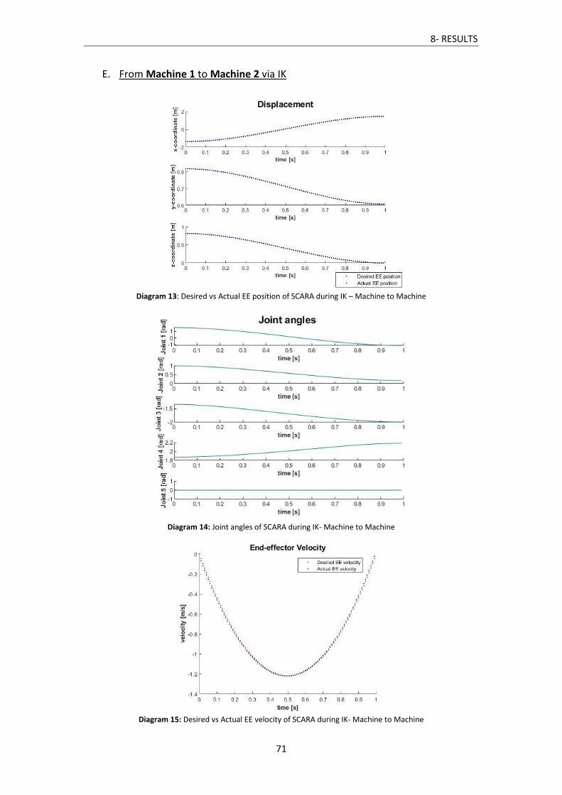
8- RESULTS
71
E. From Machine 1 to Machine 2 via IK
Diagram 13: Desired vs Actual EE position of SCARA during IK – Machine to Machine
Diagram 14: Joint angles of SCARA during IK- Machine to Machine
Diagram 15: Desired vs Actual EE velocity of SCARA during IK- Machine to Machine

8- RESULTS
72
F. From Home position to safe position before Output position via FK
Diagram 16: EE position of SCARA with FK- Home to Safe Position
Diagram 17: Joint angles of SCARA with FK- Home to Safe Position
Diagram 18: Joint velocities of SCARA with FK- Home to Safe Position

8- RESULTS
73
G. From safe position before Output position to Output via IK
Diagram 19: Desired vs Actual EE position of SCARA during IK - Safe to Output Position
Diagram 20: Joint angles of SCARA during IK- Safe to Output Position
Diagram 21: Desired vs Actual EE velocity of SCARA during IK- Safe to Output Position

8- RESULTS
74
8.3 STAUBLI RX-90
A. From Home position to Input position via IK
Diagram 22: Desired vs Actual EE position of STAUBLI during IK- Home to Input Position
Diagram 23: Joint angles of STAUBLI during IK - Home to Input Position
Diagram 24: Desired vs Actual EE velocity of STAUBLI during IK- Home to Input Position
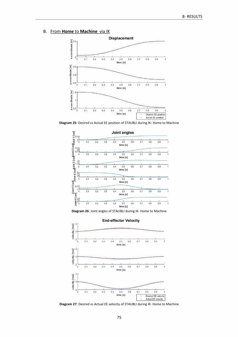
8- RESULTS
75
B. From Home to Machine via IK
Diagram 25: Desired vs Actual EE position of STAUBLI during IK- Home to Machine
Diagram 26: Joint angles of STAUBLI during IK- Home to Machine
Diagram 27: Desired vs Actual EE velocity of STAUBLI during IK- Home to Machine

8- RESULTS
76
C. Machine to Home via FK
Diagram 28: EE position of STAUBLI with FK- Machine to Home
Diagram 29: Joint angles of STAUBLI with FK- Machine to Home
Diagram 30: Joint velocities of STAUBLI with FK- Machine to Home
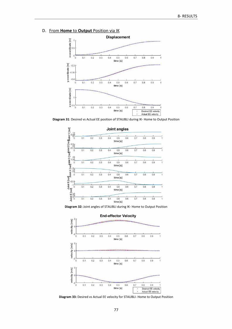
8- RESULTS
77
D. From Home to Output Position via IK
Diagram 31: Desired vs Actual EE position of STAUBLI during IK- Home to Output Position
Diagram 32: Joint angles of STAUBLI during IK- Home to Output Position
Diagram 33: Desired vs Actual EE velocity for STAUBLI- Home to Output Position

9- CONCLUSIONS AND WORK
78
9 CONCLUSIONS
AND FUTURE WORK
9.1 Contribution
This diploma thesis describes a methodology for developing a robotic biotechnology lab model
in a virtual environment. The process involved both the introduction of 3D models for the
representation of the physical space and their programming so that the moving parts –the
robots –would gain "life" and interact with the rest.
The main contribution of this work is the development of a methodology towards the
kinematical control of two different robots and two different system layouts, which can be
used as a low cost alternative to impedance control or visual servoing of the robot or to
expensive high-accuracy robots. The thesis can provide a background for expanding or even
developing other related methodologies.
Specifically covered were:
1. Model of custom made SCARA type robotic arm with fully developed kinematic
chain linkage.
2. Model of Stäubli TX2-90XL robotic arm with fully developed kinematic chain linkage.
3. Actual model of the biotechnology laboratory space with dimensions and layouts.
4. Direct and inverse kinematic analysis of the robotic arms at hand.
5. Simulation of complete experimental protocols in the virtual environment VREP.
9.2 Advantages of virtual environments
The conventional task scheduling of an industrial robot has always been based on the
experience of the operator, who was planning his orbit while in operation. This way, besides
being time consuming, it ran the risk of error, endangering the integrity of the operator, the
industrial equipment as well as the work. Nowadays, young engineers and craftsmen are
called upon to do the programming work. Due to their familiarity with virtual reality
technologies, the use of the latter in this work gives fast, reliable and secure results.
There is an obvious economic benefit, as well. Money is saved because of reduced labor hours,
failed efforts, and the damage caused by collisions. Also, such a system can be used to properly
study the installation of additional mechanical equipment in an already existing environment.

9- CONCLUSIONS AND WORK
79
9.3 Suggestions for future development
The development of the laboratory set up and the trajectory planning been successful, but
there is still room for improvement.
As far as the laboratory set up is concerned:
The experiment scenarios tested for the purposes of this thesis included only 5
machines – workstations, as part of the laboratory. These machines are the most
common found in a biotechnology laboratory and most often used to conduct
experiments. A possible extension could be to include more specialized machines in
the same laboratory set ups for the conduction experiments. For example, a Flow
Cytometer, a High-Content Screening and a Microplate Dispenser could be such
additions.
In the current project the experiments were also simulated one- by –one, meaning
that a new experiment was planned to begin right after the previous experiment was
completed. Implementing algorithms on the planning of Flexible Manufacturing could
allow for multiple experiments to take place in the laboratory at the same time.
Incorporating markers and vision systems to recognize the different microplates
found in the lab at each instant, the robot could receive multiple experiment protocols
and complete them simultaneously, increasing thus the productivity of the cell.
As far as the control of the robotic arms is concerned:
The research focused on the kinematic analysis of the robotic arms, completely
ignoring their dynamics. A dynamic simulation could be attempted to analyze the
oscillations while the robots are in operation, as well as their effect on the accuracy
of the trajectory.
A live localization system with the addition of cameras can be implemented to ensure
accuracy. An arm camera could be used to align the arm with the machine entry points
and also one camera that can spot the position of the machines and the well-plate.
These cameras can be utilized to correct position errors and give live feedback.
Experimental results from the control of the Stäubli TX2-90XL robotic arm could be
modeled on a physical level with the information provided from the virtual
environment via the language V+. To that respect, Matlab-VREP output files
concerning the position of the end-effector or the values of the joint angles at each
configuration could be passed via a V+ controller to the actual model of the Stäubli to
assess the actual behavior of the robot and if it coincides with the simulated one.

10- BIBLIOGRAPHY
80
10 BIBLIOGRAPHY
[1] R. Pauwels, H. Azijn, M. P. de Béthune, C. Claeys, and K. Hertogs, “Automated techniques in biotechnology,” Curr. Opin. Biotechnol., vol. 6, no. 1, pp. 111–117, 1995.
[2] A. Sertkaya, H. H. Wong, A. Jessup, and T. Beleche, “Key cost drivers of pharmaceutical clinical trials in the United States,” Clin. Trials, vol. 13, no. 2, pp. 117–126, Apr. 2016.
[3] L. Monostori, “Cyber-physical production systems: Roots, expectations and R&D challenges,” in Procedia CIRP, 2014, vol. 17, pp. 9–13.
[4] L. Monostori et al., “Cyber-physical systems in manufacturing,” CIRP Ann., vol. 65, no. 2, pp. 621–641, 2016.
[5] M. Smith, J., Kreutzer, S., Moeller, C., & Carlberg, “Industry 4.0. Study for the ITRE committee,” 2016.
[6] N. Shariatzadeh, T. Lundholm, L. Lindberg, and G. Sivard, “Integration of Digital Factory with Smart Factory Based on Internet of Things,” in Procedia CIRP, 2016, vol. 50, pp. 512–517.
[7] U. Bracht and T. Masurat, “The Digital Factory between vision and reality,” Comput. Ind., vol. 56, no. 4, pp. 325–333, May 2005.
[8] D. Mourtzis, N. Papakostas, D. Mavrikios, and S. Makris, “Det 2011,” no. November 2017, 2011.
[9] V. Bottazzi and J. Fonsec, “Off-line Programming Industrial Robots Based in the Information Extracted From Neutral Files Generated by the Commercial CAD Tools,” Ind. Robot. Program. Simul. Appl., 2006.
[10] Coppelia Robotics, “V-REP User Manual.” [Online]. Available: http://www.coppeliarobotics.com/helpFiles/index.html.
[11] Wikipedia, “SCARA.” [Online]. Available: https://en.wikipedia.org/wiki/SCARA. [Accessed: 08-Aug-2019].
[12] Cyan-Tec, “When to use a SCARA Robot.” [Online]. Available: https://cyan-tec.com/laser-systems/when-to-use-a-scara-robot.
[13] Γ. Χ. Βοσνιάκος, Συστήματα Κατεργασιών Ι, Πρόχειρες σημειώσεις. .
[14] H. Fleischer and K. Thurow, “Automation Solutions for Analytical Measurements: Concepts and Applications.” [Online]. Available: https://books.google.gr/books?id=Mlw6DwAAQBAJ&pg=PA171&lpg=PA171&dq=gripper+fingers+for+microplate&source=bl&ots=WlkBUNulqG&sig=ACfU3U24QXQ_rKo_7Q8UWz5Ui_lkVcCC_A&hl=el&sa=X&ved=2ahUKEwiotebAyrLlAhVOecAKHQI1D_oQ6AEwEXoECAgQAQ#v=onepage&q=gripper fingers f. [Accessed: 23-Oct-2019].
10- BIBLIOGRAPHY
81
[15] “PTM-Präzisionstechnik.” [Online]. Available: http://www.ptm-automation.de/HomePTMPräzisionstechnik/OurCompany/Products/ServoGripperLaboratoryAutomation.aspx.
[16] “PatentSwarm.” [Online]. Available: https://patentswarm.com/patents/US7670555B2.
[17] P. Kosky, R. Balmer, W. Keat, and G. Wise, “Manufacturing Engineering,” in Exploring Engineering, Elsevier, 2013, pp. 205–235.
[18] V. Manthou and M. Vlachopoulou, “Agile Manufacturing Strategic Options,” in Agile Manufacturing: The 21st Century Competitive Strategy, Elsevier, 2001, pp. 685–702.
[19] T. Yang, B. A. Peters, and M. Tu, “Layout design for flexible manufacturing systems considering single-loop directional flow patterns,” Eur. J. Oper. Res., vol. 164, no. 2, pp. 440–455, Jul. 2005.
[20] J. J. Craig, Introduction to ROBOTICS mechanics and control, 3rd ed. Pearson Education International, 2005.
[21] B. Siciliano, L. Sciavicco, L. Villani, and G. Oriolo, Robotics : modelling, planning and control. Springer, 2009.
[22] S. Chiaverini, B. Siciliano, and O. Egeland, “Review of the Damped Least-Squares Inverse Kinematics with Experiments on an Industrial Robot Manipulator,” IEEE Trans. Control Syst. Technol., vol. 2, no. 2, pp. 123–134, 1994.
[23] R. Krasňanský, P. Valach, D. Soós, and J. Zarbakhsh, “Reference trajectory tracking for a multi-DOF robot arm,” Arch. Control Sci., vol. 25, no. 4, pp. 513–527, 2015.
[24] D. Di Vito, C. Natale, and G. Antonelli, “A Comparison of Damped Least Squares Algorithms for Inverse Kinematics of Robot Manipulators,” IFAC-PapersOnLine, vol. 50, no. 1, pp. 6869–6874, 2017.
[25] X. Zhao, M. Wang, N. Liu, and Y. Tang, “Trajectory Planning for 6-DOF Robotic Arm Based on Quintic Polynormial,” vol. 134, no. Caai, pp. 115–118, 2017.
[26] C. Feng, G. Gao, and Y. Cao, “Kinematic modeling and verification for a SCARA robot,” no. Icmemtc, pp. 918–921, 2016.
[27] “ROS URDF.” [Online]. Available: https://wiki.ros.org/urdf.

82
APPENDIX
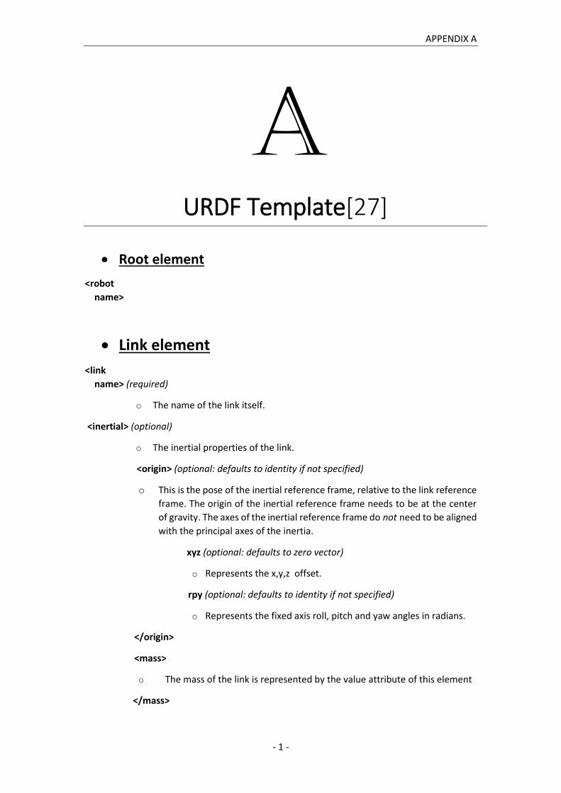
APPENDIX A
- 1 -
A URDF Template[27]
Root element
<robot
name>
Link element
<link
name> (required)
o The name of the link itself.
<inertial> (optional)
o The inertial properties of the link.
<origin> (optional: defaults to identity if not specified)
o This is the pose of the inertial reference frame, relative to the link reference
frame. The origin of the inertial reference frame needs to be at the center
of gravity. The axes of the inertial reference frame do not need to be aligned
with the principal axes of the inertia.
xyz (optional: defaults to zero vector)
o Represents the x,y,z offset.
rpy (optional: defaults to identity if not specified)
o Represents the fixed axis roll, pitch and yaw angles in radians.
</origin>
<mass>
o The mass of the link is represented by the value attribute of this element
</mass>
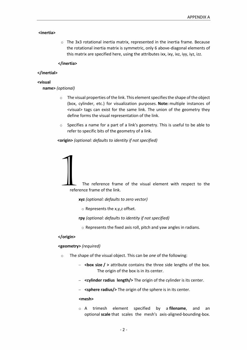
APPENDIX A
- 2 -
<inertia>
o The 3x3 rotational inertia matrix, represented in the inertia frame. Because
the rotational inertia matrix is symmetric, only 6 above-diagonal elements of
this matrix are specified here, using the attributes ixx, ixy, ixz, iyy, iyz, izz.
</inertia>
</inertial>
<visual
name> (optional)
o The visual properties of the link. This element specifies the shape of the object
(box, cylinder, etc.) for visualization purposes. Note: multiple instances of
<visual> tags can exist for the same link. The union of the geometry they
define forms the visual representation of the link.
o Specifies a name for a part of a link's geometry. This is useful to be able to
refer to specific bits of the geometry of a link.
<origin> (optional: defaults to identity if not specified)
1 The reference frame of the visual element with respect to the
reference frame of the link.
xyz (optional: defaults to zero vector)
o Represents the x,y,z offset.
rpy (optional: defaults to identity if not specified)
o Represents the fixed axis roll, pitch and yaw angles in radians.
</origin>
<geometry> (required)
o The shape of the visual object. This can be one of the following:
<box size / > attribute contains the three side lengths of the box.
The origin of the box is in its center.
<cylinder radius length/> The origin of the cylinder is its center.
<sphere radius/> The origin of the sphere is in its center.
<mesh>
o A trimesh element specified by a filename, and an
optional scale that scales the mesh's axis-aligned-bounding-box.

APPENDIX A
- 3 -
The recommended format for best texture and color support is
Collada .dae files, though .stl files are also supported. The mesh file
is not transferred between machines referencing the same model. It
must be a local file.
</mesh>
<material
name> (optional)
o The material of the visual element. It is allowed to specify a material
element outside of the 'link' object, in the top level 'robot' element.
From within a link element you can then reference the material by
name.
</material>
<color> (optional)
o rgba The color of a material specified by set of four numbers
representing red/green/blue/alpha, each in the range of [0,1].
</color>
<texture> (optional)
o The texture of a material is specified by a filename
</texture>
</geometry>
</visual>
<collision
name> (optional)
o The collision properties of a link. Note that this can be different from the
visual properties of a link, for example, simpler collision models are often
used to reduce computation time. Note: multiple instances of <collision> tags
can exist for the same link. The union of the geometry they define forms the
collision representation of the link.
o Specifies a name for a part of a link's geometry. This is useful to be able to
refer to specific bits of the geometry of a link.
<origin> (optional: defaults to identity if not specified)
o The reference frame of the collision element, relative to the reference frame
of the link.
xyz (optional: defaults to zero vector)
o Represents the x,y,z offset.
rpy (optional: defaults to identity if not specified)

APPENDIX A
- 4 -
o Represents the fixed axis roll, pitch and yaw angles in radians.
</origin>
<geometry>
o See the geometry description in the above visual element.
</geometry>
</collision>
</link>
Joint element
<joint
name (required)
o Specifies a unique name of the joint
type >(required)
o Specifies the type of joint, where type can be one of the following:
revolute - a hinge joint that rotates along the axis and has a limited
range specified by the upper and lower limits.
continuous - a continuous hinge joint that rotates around the axis
and has no upper and lower limits.
prismatic - a sliding joint that slides along the axis, and has a limited
range specified by the upper and lower limits.
fixed - This is not really a joint because it cannot move. All degrees
of freedom are locked. This type of joint does not require the axis,
calibration, dynamics, limits or safety_controller.
floating - This joint allows motion for all 6 degrees of freedom.
planar - This joint allows motion in a plane perpendicular to the axis.
<origin> (optional: defaults to identity if not specified)
o This is the transform from the parent link to the child link. The joint is
located at the origin of the child link, as shown in Figure 11.
xyz (optional: defaults to zero vector)
o Represents the x,y,z offset. All positions are specified in meters.
rpy (optional: defaults 'to zero vector 'if not specified)
o Represents the rotation around fixed axis: first roll around x, then
pitch around y and finally yaw around z. All angles are specified in
radians.
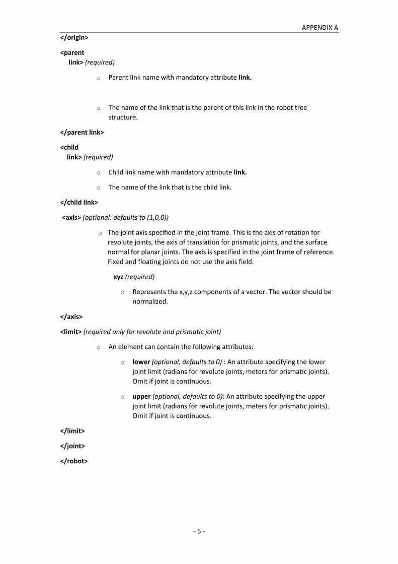
APPENDIX A
- 5 -
</origin>
<parent
link> (required)
o Parent link name with mandatory attribute link.
o The name of the link that is the parent of this link in the robot tree
structure.
</parent link>
<child
link> (required)
o Child link name with mandatory attribute link.
o The name of the link that is the child link.
</child link>
<axis> (optional: defaults to (1,0,0))
o The joint axis specified in the joint frame. This is the axis of rotation for
revolute joints, the axis of translation for prismatic joints, and the surface
normal for planar joints. The axis is specified in the joint frame of reference.
Fixed and floating joints do not use the axis field.
xyz (required)
o Represents the x,y,z components of a vector. The vector should be
normalized.
</axis>
<limit> (required only for revolute and prismatic joint)
o An element can contain the following attributes:
o lower (optional, defaults to 0) : An attribute specifying the lower
joint limit (radians for revolute joints, meters for prismatic joints).
Omit if joint is continuous.
o upper (optional, defaults to 0): An attribute specifying the upper
joint limit (radians for revolute joints, meters for prismatic joints).
Omit if joint is continuous.
</limit>
</joint>
</robot>

APPENDIX B
- 6 -
B TECHNICAL SPECIFICATIONS OF
EQUIPMENT AND CONSUMABLES
B1) Staubli TX2-90XL [Source: Staubli]

APPENDIX B
- 7 -
B2) Custom experoment Gripper
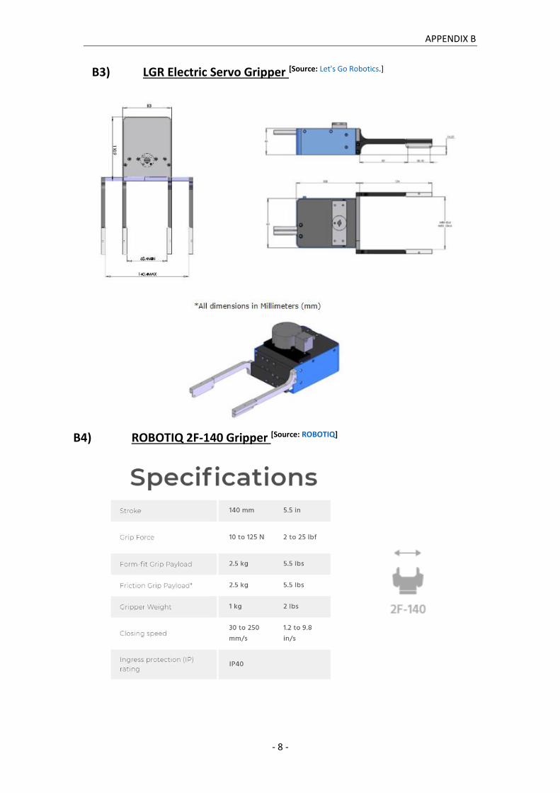
APPENDIX B
- 8 -
B3) LGR Electric Servo Gripper [Source: Let's Go Robotics.]
B4) ROBOTIQ 2F-140 Gripper [Source: ROBOTIQ]

APPENDIX B
- 9 -
B5) Liquid Handler – Opentrons [Source: Opentrons]
Dimensions [mm]
Height 630
Depth 570
Width 660
B6) Centrifuge - ROTANTA 460 Robotic [Source: Hettich]

APPENDIX B
- 10 -
B7) Freezer -STR44 [Source: Liconic]
B8) Incubator- STR240 [Source: Liconic]
B9) Plate Reader- EnVision 2105 [Source: Perkin Elmer]
Dimensions [mm]
Height 580
Depth 550
Width 420


APPENDIX C
- 13 -
C MATLAB CODE
SCARA FILES main_SCARA.m…………………………………………………………………………………………………………...…14
USER_INPUT.m……………………………………………………………………………………………………………….15
TrajParam.m….…………………………………………………………………………………………………………….…15
Cartesian_Traj.m…………………………………………………………………………………………………………….16
Joint_Traj.m…………..……………………………………………………………………………………………….……...16
SCENE_ELEMENTS.m………………………………………………………………………………………………….…..16
EXECUTE_EXPERIMENT.m…………………………………………………………………………………………….…19
CHECK_HOME.m…..……………………………………………………………………………………………………..…20
Joint_Trajall.m…..………………………………………………………………………………………………………...…22
SCARAexetraj.m….………………………………………………………………………………………………………..…26
SCARAplatetraj.m……………………………………………………………………………………………………..…….31
OPEN_GRIPPER.m……………………………………………………………………………………………………..…….36
CLOSE…GRIPPER.m……………………………………………………………………………………….………………….37
PLATE.m….……………………………………………………………………………………………………….………………38
TURN_PLATE.m…………………………………………………………………………………………………..……………39
MACHINES.m……………………………………………………………………………………………………………………40
OUTPUT.m….………………………………………………………………………………………………..…….……………41
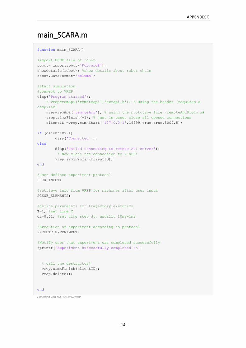
APPENDIX C
- 14 -
main_SCARA.m
function main_SCARA()
%import URDF file of robot
robot= importrobot('Rob.urdf');
showdetails(robot); %show details about robot chain
robot.DataFormat='column';
%start simulation
%connect to VREP
disp('Program started');
% vrep=remApi('remoteApi','extApi.h'); % using the header (requires a
compiler)
vrep=remApi('remoteApi'); % using the prototype file (remoteApiProto.m)
vrep.simxFinish(-1); % just in case, close all opened connections
clientID =vrep.simxStart('127.0.0.1',19999,true,true,5000,5);
if (clientID>-1)
disp('Connected ');
else
disp('Failed connecting to remote API server');
% Now close the connection to V-REP:
vrep.simxFinish(clientID);
end
%User defines experiment protocol
USER_INPUT;
%retrieve info from VREP for machines after user input
SCENE_ELEMENTS;
%define parameters for trajectory execution
T=1; %set time T
dt=0.01; %set time step dt, usually 10ms-1ms
%Execution of experiment according to protocol
EXECUTE_EXPERIMENT;
%Notify user that experiment was completed successfully
fprintf('Experiment successfully completed \n')
% call the destructor!
vrep.simxFinish(clientID);
vrep.delete();
end
Published with MATLAB® R2018a

APPENDIX C
- 15 -
USER_INPUT.m
%%%%%%%% USER INPUT %%%%%%%%%%%
%ask user for machine input- experiment protocol
machine={};
i=1;
while (1)
prompt=input('Input working station \n', 's');
if strcmp (prompt, 'stop')
break
end
machine{i,1}=prompt;
i=i+1;
end
Published with MATLAB® R2018a TrajParam.m
function [x] = TrajParam(T)
% find time-law (3rd order polynomial), [a b c d] only need one time
computation
% s= a*t^3+ b*t^2+ c*t+d
% sd= 3*a*t^2+ 2*b*t+c
%define constraints
% s(0)=0 ; s(T)= 1;
% sd(0)= 0 ; sd(T)=0;
%x= [a b c d]
%Ax=b
A= [0 0 0 1;
T^3 T^2 T 1;
0 0 1 0;
3*T^2 2*T 1 0];
B = [0; 1; 0; 0];
x= pinv(A)* B ;
end
Published with MATLAB® R2018a

APPENDIX C
- 16 -
Cartesian_Traj.m
function [P, v, theta, thetad]=Cartesian_Traj(P_o,P_f,theta_i, theta_f,t,x)
%calculate cartesian trajectory
s= x(1)*t^3 + x(2)*t^2+ x(3)*t+ x(4);
sd= 3*x(1)*t^2 + 2*x(2)*t+x(3);
P= (P_f-P_o)*s+P_o ;
v=(P_f-P_o)*sd ;
theta= (theta_f-theta_i)*s+theta_i ;
thetad=(theta_f-theta_i)*sd ;
end
Published with MATLAB® R2018a
Joint_Traj.m
function [q_d,qdot]=Joint_Traj(q_i,q_f,t,x)
%calculate joint trajectory
s= x(1)*t^3 + x(2)*t^2+ x(3)*t+ x(4);
sd= 3*x(1)*t^2 + 2*x(2)*t+x(3);
q_d= (q_f-q_i)*s+q_i ;
qdot=(q_f-q_i)*sd ;
end
Published with MATLAB® R2018a
SCENE_ELEMENTS.m
%%%%%%%%%%%%% HANDLES %%%%%%%%%%%%%%%
%get handle for world frame-all machines are relative to this frame
[~,Base_frame]=vrep.simxGetObjectHandle(clientID,'world_visual',vrep.simx_op
mode_blocking);
%get handles for other necessary components of simulation
[~,Plate_frame]=vrep.simxGetObjectHandle(clientID,'Plate_frame',vrep.simx_op
mode_blocking);
[~,EE]=vrep.simxGetObjectHandle(clientID,'ee_link_dummy',vrep.simx_opmode_bl
ocking);

APPENDIX C
- 17 -
[~,ee]=vrep.simxGetObjectHandle(clientID,'ee_link_visual',vrep.simx_opmode_b
locking);
[~,Input_Tech]=vrep.simxGetObjectHandle(clientID,'Input_Tech',vrep.simx_opmo
de_blocking);
[~,Output_Tech]=vrep.simxGetObjectHandle(clientID,'Output_Tech',vrep.simx_op
mode_blocking);
[~,Turn]=vrep.simxGetObjectHandle(clientID,'BaseArm_JointRot',vrep.simx_opmo
de_blocking);
[~,ProxS]=vrep.simxGetObjectHandle(clientID,'ProxS',vrep.simx_opmode_blockin
g);
%get handles joints
[~,Joint1]=vrep.simxGetObjectHandle(clientID,'Arm_Joint1',vrep.simx_opmode_b
locking);
[~,Joint2]=vrep.simxGetObjectHandle(clientID,'Arm_Joint2',vrep.simx_opmode_b
locking);
[~,BaseJ1]=vrep.simxGetObjectHandle(clientID,'BaseArm_Joint1',vrep.simx_opmo
de_blocking);
[~,BaseJ2]=vrep.simxGetObjectHandle(clientID,'BaseArm_Joint2',vrep.simx_opmo
de_blocking);
[~,Joint3]=vrep.simxGetObjectHandle(clientID,'Arm_Joint3',vrep.simx_opmode_b
locking);
[~,Grip1]=vrep.simxGetObjectHandle(clientID,'Gripper_JointDx',vrep.simx_opmo
de_blocking);
[~,Grip2]=vrep.simxGetObjectHandle(clientID,'Gripper_JointSx',vrep.simx_opmo
de_blocking);
[~,Turn]=vrep.simxGetObjectHandle(clientID,'BaseArm_JointRot',vrep.simx_opmo
de_blocking);
%get joint values from VREP
[~,J1]=vrep.simxGetJointPosition(clientID,BaseJ1,vrep.simx_opmode_blocking);
[~,J2]=vrep.simxGetJointPosition(clientID,BaseJ2,vrep.simx_opmode_blocking);
[~,J3]=vrep.simxGetJointPosition(clientID,Joint1,vrep.simx_opmode_blocking);
[~,J4]=vrep.simxGetJointPosition(clientID,Joint2,vrep.simx_opmode_blocking);
[~,J5]=vrep.simxGetJointPosition(clientID,Joint3,vrep.simx_opmode_blocking);
[~,GripR]=vrep.simxGetJointPosition(clientID,Grip1,vrep.simx_opmode_blocking
);
[~,GripL]=vrep.simxGetJointPosition(clientID,Grip2,vrep.simx_opmode_blocking
);
%INITIAL JOINT CONFIGURATION
q= [J1; J2;J3;J4;J5];
%set home configuration of robot-it always returns here
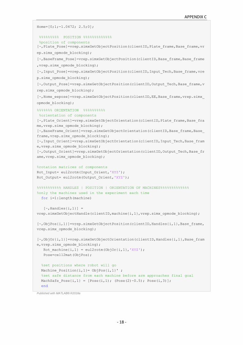
APPENDIX C
- 18 -
Home=[0;1;-1.0472; 2.5;0];
%%%%%%%%% POSITION %%%%%%%%%%%%%
%position of components
[~,Plate_Pose]=vrep.simxGetObjectPosition(clientID,Plate_frame,Base_frame,vr
ep.simx_opmode_blocking);
[~,BaseFrame_Pose]=vrep.simxGetObjectPosition(clientID,Base_frame,Base_frame
,vrep.simx_opmode_blocking);
[~,Input_Pose]=vrep.simxGetObjectPosition(clientID,Input_Tech,Base_frame,vre
p.simx_opmode_blocking);
[~,Output_Pose]=vrep.simxGetObjectPosition(clientID,Output_Tech,Base_frame,v
rep.simx_opmode_blocking);
[~,Home_eepose]=vrep.simxGetObjectPosition(clientID,EE,Base_frame,vrep.simx_
opmode_blocking);
%%%%%%% ORIENTATION %%%%%%%%%%
%orientation of components
[~,Plate_Orient]=vrep.simxGetObjectOrientation(clientID,Plate_frame,Base_fra
me,vrep.simx_opmode_blocking);
[~,BaseFrame_Orient]=vrep.simxGetObjectOrientation(clientID,Base_frame,Base_
frame,vrep.simx_opmode_blocking);
[~,Input_Orient]=vrep.simxGetObjectOrientation(clientID,Input_Tech,Base_fram
e,vrep.simx_opmode_blocking);
[~,Output_Orient]=vrep.simxGetObjectOrientation(clientID,Output_Tech,Base_fr
ame,vrep.simx_opmode_blocking);
%rotation matrices of components
Rot_Input= eul2rotm(Input_Orient,'XYZ');
Rot_Output= eul2rotm(Output_Orient,'XYZ');
%%%%%%%%%%% HANDLES | POSITION | ORIENTATION OF MACHINES%%%%%%%%%%%%%
%only the machines used in the experiment each time
for i=1:length(machine)
[~,Handles{i,1}] =
vrep.simxGetObjectHandle(clientID,machine{i,1},vrep.simx_opmode_blocking);
[~,ObjPos{i,1}]=vrep.simxGetObjectPosition(clientID,Handles{i,1},Base_frame,
vrep.simx_opmode_blocking);
[~,ObjOr{i,1}]=vrep.simxGetObjectOrientation(clientID,Handles{i,1},Base_fram
e,vrep.simx_opmode_blocking);
Rot_machine{i,1} = eul2rotm(ObjOr{i,1},'XYZ');
Pose=cell2mat(ObjPos);
%set positions where robot will go
Machine_Position{i,1}= ObjPos{i,1}' ;
%set safe distance from each machine before arm approaches final goal
MachSafe_Pose{i,1} = [Pose(i,1); (Pose(2)-0.5); Pose(i,3)];
end
Published with MATLAB® R2018a

APPENDIX C
- 19 -
EXECUTE_EXPERIMENT.m
%%%%% EXECUTION OF EXPERIMENT %%%%%%%%
% make sure robot is not at a non-desirable position
CHECK_HOME(robot, q,T,dt,Home, Rot_Input,BaseJ1,BaseJ2, Joint1,
Joint2,EE,Grip1,Grip2, Input_Pose );
%%%%% EXECUTION OF EXPERIMENT %%%%%%
for i=1:length(machine)
rot_m= Rot_machine{i,1};
if strcmp (machine{i,1}, 'Opentrons')
PLATE (robot, q,T,dt,Plate_frame,Base_frame,Home, BaseJ1, BaseJ2, Joint1,
Joint2,EE, Grip1, Grip2, Turn);
MACHINES(robot, q, T,dt,i, Machine_Position, MachSafe_Pose, rot_m,
BaseJ1,BaseJ2, Joint1, Joint2,EE, Grip1, Grip2, Home);
PLATE (robot, q,T,dt,Plate_frame,Base_frame,Home, BaseJ1, BaseJ2, Joint1,
Joint2,EE, Grip1, Grip2, Turn);
else
MACHINES(robot, q, T,dt,i, Machine_Position, MachSafe_Pose, rot_m,
BaseJ1,BaseJ2, Joint1, Joint2,EE, Grip1, Grip2, Home);
end
%
i=i+1;
end
%Plate returns to technician-output
OUTPUT (robot, q,T,dt, Rot_Output,Output_Pose,BaseJ1,BaseJ2, Joint1,
Joint2,EE, Grip1, Grip2, Home);
Published with MATLAB® R2018a

APPENDIX C
- 20 -
CHECK_HOME.m
function CHECK_HOME(robot, q,T,dt,Home, Rot_Input,BaseJ1,BaseJ2, Joint1,
Joint2,EE,Grip1,Grip2, Input_Pose )
%%%%%%CHECK HOME%%%%%%
%checks if robot is in home position
%if yes user is notified
%if not it is commanded to go to home position before the start of the
experiment
%connect to VREP
% vrep=remApi('remoteApi','extApi.h'); % using the header (requires a
compiler)
vrep=remApi('remoteApi'); % using the prototype file (remoteApiProto.m)
vrep.simxFinish(-1); % just in case, close all opened connections
clientID =vrep.simxStart('127.0.0.1',19999,true,true,5000,5);
if (clientID>-1)
disp('')
else
% close the connection to V-REP and notify user
vrep.simxFinish(clientID);
end
if q(1)==0 && q(2)== 1 && q(3)==-1.0472 && q(4)==2.5 && q(5)==0
printf('Robot is in Home Position-Ready to start experiment')
else
%return robot to home joint configuration
q_f= Home;
q= Joint_Trajall(robot,q,T,dt,q_f,BaseJ1,BaseJ2, Joint1, Joint2, EE);
end
prompt='Do you wish to continue to experiment? Y/N [Y]:';
str = input(prompt,'s');
if isempty(str) || str=='Y'
str = 'Y';
%start with experiment and notify user
fprintf('Experiment started \n')
pause(1);
%first step is to take plate from technician-input
%set joint configuration above input window
q_f= [1.6;1;0.4; 1.3;0];
q= Joint_Trajall(robot,q,T,dt,q_f,BaseJ1,BaseJ2, Joint1, Joint2, EE);
% move to grab plate
OPEN_GRIPPER(Grip1, Grip2);
rot_m= Rot_Input;
P_f= (Input_Pose)';

APPENDIX C
- 21 -
q= SCARAexetraj(robot,q,T,dt,P_f,rot_m,BaseJ1,BaseJ2, Joint1, Joint2,EE);
CLOSE_GRIPPER(Grip1, Grip2);
% move again to safe configuration above input window
%return to home configuration before proceeding
q_f= [1.6;1;0.4; 1.3;0];
q= Joint_Trajall(robot,q,T,dt,q_f,BaseJ1,BaseJ2, Joint1, Joint2,
EE);
q_f= Home;
q= Joint_Trajall(robot,q,T,dt,q_f,BaseJ1,BaseJ2, Joint1, Joint2,
EE);;
else
error('Experiment interrupted by user')
end
% call the destructor!
vrep.simxFinish(clientID);
vrep.delete();
end
Published with MATLAB® R2018a

APPENDIX C
- 22 -
Joint_Trajall.m
function q= Joint_Trajall(robot,q,T,dt,q_f,BaseJ1,BaseJ2, Joint1, Joint2,
EE)
%connect to VREP
% vrep=remApi('remoteApi','extApi.h'); % using the header (requires a
compiler)
vrep=remApi('remoteApi'); % using the prototype file (remoteApiProto.m)
vrep.simxFinish(-1); % just in case, close all opened connections
clientID =vrep.simxStart('127.0.0.1',19999,true,true,5000,5);
if (clientID>-1)
disp('Connected ');
else
disp('Failed connecting to remote API server');
end
%Retrieve current joint configuration
q_i= [ q(1); q(2); q(3); q(4); q(5)];
%offset between visual EE and actual EE
T_dummy_e=[1 0 0 0.071004;0 1 0 0.029014 ; 0 0 1 0 ;0 0 0 1];
%parameters for trajectory
% T=1; %set time T
x= TrajParam(T);
% dt= 0.01; %set time step, usually 10ms-1ms
t=0;
c=1;
while t<= T
%homogenous transformation for robot chain
T_e= getTransform(robot,double(q),'ee_link');
%transformation from visual EE to actual EE
T_final= T_e* T_dummy_e;
P_i= T_final(1:3,4);
%get path between initial and desired configuration
[q_d,qdot]=Joint_Traj(q_i,q_f,t,x);
%joint position at t+dt
q= q+qdot*dt;
for j=3:5
q(j)=atan2(sin(q(j)),cos(q(j)));
end
%%%%%%%%%%%%%%%%%%%%%%%%%%%%%%%%%%%%%%%%%%%%
%save the values for position and velocity for later plotting
timeV(c)= t;
X_act(c,:)= P_i(1);
Y_act(c,:)=P_i(2);
Z_act(c,:)= P_i(3);

APPENDIX C
- 23 -
q1(c,:)= q(1);
q2(c,:)= q(2);
q3(c,:)= q(3);
q4(c,:)= q(4);
q5(c,:)= q(5);
qd1(c,:)= qdot(1);
qd2(c,:)= qdot(2);
qd3(c,:)= qdot(3);
qd4(c,:)= qdot(4);
qd5(c,:)= qdot(5);
c=c+1 ;
%%%%%%%%%%%%%%%%%%%%%%%%%%%%%%%%%%%%%%%%%%%%
t=t+dt;
% update visual robot configuration
[~]=vrep.simxPauseCommunication(clientID,1);
[J1]=vrep.simxSetJointPosition(clientID,BaseJ1,q(1),vrep.simx_opmode_oneshot
);
[J2]=vrep.simxSetJointPosition(clientID,BaseJ2,q(2),vrep.simx_opmode_oneshot
);
[J3]=vrep.simxSetJointPosition(clientID,Joint1,q(3),vrep.simx_opmode_oneshot
);
[J4]=vrep.simxSetJointPosition(clientID,Joint2,q(4),vrep.simx_opmode_oneshot
);
[J5]=vrep.simxSetJointPosition(clientID,EE,q(5),vrep.simx_opmode_oneshot);
[~]=vrep.simxPauseCommunication(clientID,0);
pause(dt);
end
%%%% POSITION PLOTS %%%%
figure()
%plot x,y,z of trajectory
subplot(3,1,1);
hold on
plot (timeV,X_act)
title('Actual End-Effector Displacement (FK)' , 'FontSize',14)
ylabel('x-coordinate [m]','FontWeight','Bold')
xlabel('time [s]','FontWeight','Bold')
subplot(3,1,2);
hold on
plot (timeV,Y_act)
ylabel('y-coordinate [m]','FontWeight','Bold')
xlabel('time [s]','FontWeight','Bold')
subplot(3,1,3);
hold on
plot (timeV,Z_act)
hold off
ylabel('z-coordinate [m]','FontWeight','Bold')
xlabel('time [s]','FontWeight','Bold')

APPENDIX C
- 24 -
%%%% JOINT PLOTS %%%%%
figure()
subplot(5,1,1);
hold on
plot (timeV,q1)
title('Joint angles (FK)' , 'FontSize',14)
ylabel('Joint 1 [rad]','FontWeight','Bold')
xlabel('time [s]','FontWeight','Bold')
subplot(5,1,2);
hold on
plot (timeV,q2)
ylabel('Joint 2 [rad]','FontWeight','Bold')
xlabel('time [s]','FontWeight','Bold')
subplot(5,1,3);
hold on
plot (timeV,q3)
ylabel('Joint 3 [rad]','FontWeight','Bold')
xlabel('time [s]','FontWeight','Bold')
subplot(5,1,4);
hold on
plot (timeV,q4)
ylabel('Joint 4 [rad]','FontWeight','Bold')
xlabel('time [s]','FontWeight','Bold')
subplot(5,1,5);
hold on
plot (timeV,q5)
ylabel('Joint 5 [rad]','FontWeight','Bold')
xlabel('time [s]','FontWeight','Bold')
hold off
%%%% VELOCITY PLOTS %%%%%
figure()
subplot(5,1,1);
hold on
plot (timeV,qd1)
title('Joint velocities (FK)' , 'FontSize',14)
ylabel('Joint 1 [rad/s]','FontWeight','Bold')
xlabel('time [s]','FontWeight','Bold')
subplot(5,1,2);
hold on
plot (timeV,qd2)
ylabel('Joint 2 [rad/s]','FontWeight','Bold')
xlabel('time [s]','FontWeight','Bold')
subplot(5,1,3);
hold on
plot (timeV,qd3)
ylabel('Joint 3 [rad/s]','FontWeight','Bold')
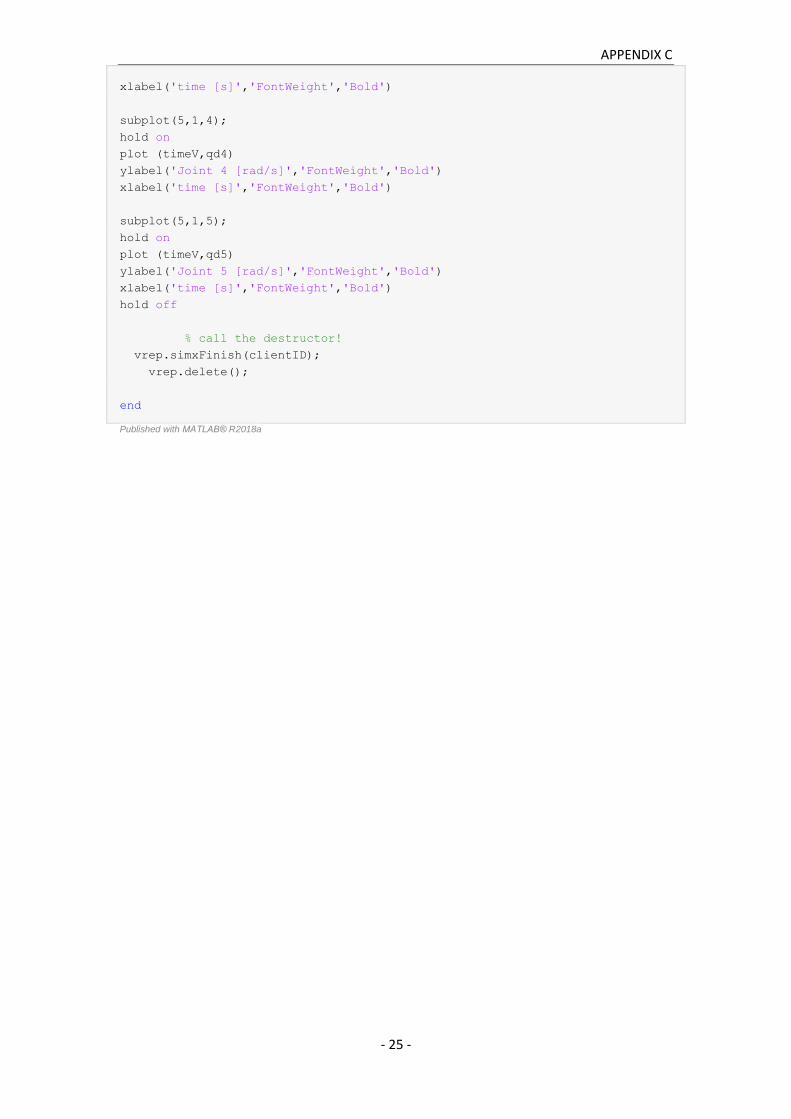
APPENDIX C
- 25 -
xlabel('time [s]','FontWeight','Bold')
subplot(5,1,4);
hold on
plot (timeV,qd4)
ylabel('Joint 4 [rad/s]','FontWeight','Bold')
xlabel('time [s]','FontWeight','Bold')
subplot(5,1,5);
hold on
plot (timeV,qd5)
ylabel('Joint 5 [rad/s]','FontWeight','Bold')
xlabel('time [s]','FontWeight','Bold')
hold off
% call the destructor!
vrep.simxFinish(clientID);
vrep.delete();
end
Published with MATLAB® R2018a

APPENDIX C
- 26 -
SCARAexetraj.m
function q= SCARAexetraj(robot,q,T,dt,P_f,rot_m,BaseJ1,BaseJ2, Joint1,
Joint2,EE)
%start simulation
%connect to VREP
% vrep=remApi('remoteApi','extApi.h'); % using the header (requires a
compiler)
vrep=remApi('remoteApi'); % using the prototype file (remoteApiProto.m)
vrep.simxFinish(-1); % just in case, close all opened connections
clientID =vrep.simxStart('127.0.0.1',19999,true,true,5000,5);
if (clientID>-1)
disp('')
else
% close the connection to V-REP and notify user
vrep.simxFinish(clientID);
end
%offset between visual EE and actual EE
T_dummy_e=[1 0 0 0.071004;0 1 0 0.029014 ; 0 0 1 0 ;0 0 0 1];
%homogenous transformation for robot chain
Trans= getTransform(robot,double(q),'ee_link');
%Transformation from visual EE to actual EE
T_fi= Trans* T_dummy_e;
P_o= T_fi(1:3,4);
%parameters for trajectory
% T=1; %set time T
x= TrajParam(T);
% dt= 0.01; %set time step, usually 10ms-1ms
t=0;
c=1;
%%%%%% Follow Trajectory %%%%%%%
while t<= T
%homogenous transformation for robot chain
T_e= getTransform(robot,double(q),'ee_link');
%transformation from visual EE to actual EE
T_final= T_e* T_dummy_e;
P_i= T_final(1:3,4);
%rotation matrix of EE wrt to base frame
Rot_EE= T_final(1:3,1:3);
%%%%% ORIENTATION ERROR %%%%%
%angle-axis representation (Sicilliano et.al)

APPENDIX C
- 27 -
R_err =transpose(Rot_EE)* (rot_m);
r_theta =rotm2axang(R_err);
r= r_theta(1, 1:3); %r wrt Rot_init
theta_f= r_theta(1, 4);
r= (Rot_EE)* transpose(r); %r wrt base frame
theta_i=0;
%elements (vectors) for Re(Rot_EE)computed from joint variables
ne= Rot_EE(:,1);
se= Rot_EE(:,2);
ae= Rot_EE(:,3);
%elements (vectors) for Rd(rot_m)
nd= rot_m(:,1);
sd= rot_m(:,2);
ad= rot_m(:,3);
%after differentiating eo wrt time
L= (-
0.5)*((nd/dt)*(nd')*(ne/dt)*(ne')+(sd/dt)*(sd')*(se/dt)*(se')+(ad/dt)*(ad')*
(ae/dt)*(ae'));
%get trajectory between initial and desired ending point
[P, v, theta, thetad]=Cartesian_Traj(P_o,P_f,theta_i, theta_f,t,x);
w= thetad*r;
wd=(L\((L')*w));
eoo= r*sin(theta);
%positive values Ko, Kp
Ko=(1/dt-10);
Kp=(1/dt-10);
%%%% ERRORS %%%%
eo= L\(Ko*eoo); %orientation error (only around z)
ep= Kp*(P-P_i); %position error
e= [ep ; eo(3)];
%%%%% JACOBIAN %%%%%
%calculate geometric jacobian
Jac_rev = geometricJacobian(robot,double(q),'ee_link');
%reverse rows
%Matlab default (first rotation, second transaltion)
Jac= [Jac_rev(4:6,:);Jac_rev(1:3,:)] ;
%linear velocity, keep x,y,z
%orientation in z axis
J= [Jac(1:3,:) ; Jac(6,:)];
%damping factor λ via SVD
[~,S,~] = svd(J);
diagS=diag(S);
sigma=min(diagS);
lamdamax=0.04;
eps= 10e-4;
APPENDIX C
- 28 -
if sigma >= eps
lamda = 0;
else
lamda= sqrt((1- ((sigma/eps)^2)*(lamdamax^2)));
end
%%%%% QUADRATIC PROGRAMMING %%%%%
%set lower-upper bounds for quadprog
q_min=[-1.9;0;-2.1;-2.5;0];
q_max= [1.8;1.9;2.1;2.5;0];
lb=(q_min-q)/dt;
ub=(q_max-q)/dt;
%Solving IK
%quadratic programming
H=(J'*J +((lamda)^2)*eye(5,5));
b=([v;wd(3)]+ e);
f=-(b')*J ;
options = optimset('Display', 'off');
qd = quadprog(double(H),double(f),[],[],[],[],double(lb),double(ub),[],
options);
ve= J*qd;
q= q+qd*dt; %joint position at t+dt
for j=3:5
q(j)=atan2(sin(q(j)),cos(q(j)));
end
%%%%%%%%%%%%%%%%%%%%%%%%%%%%%%%%%%%%%%%%%%%%
%save the values for position and velocity for later plotting
timeV(c)= t;
X_des(c,:)= P(1);
Y_des(c,:)= P(2);
Z_des(c,:)= P(3);
X_act(c,:)= P_i(1);
Y_act(c,:)= P_i(2);
Z_act(c,:)= P_i(3);
% v1_des(c,:)= v(1);
% v2_des(c,:)= v(2);
v3_des(c,:)= v(3);
% v1_act(c,:)= ve(1);
% v2_act(c,:)= ve(2);
v3_act(c,:)= ve(3);
q1(c,:)= q(1);
q2(c,:)= q(2);
q3(c,:)= q(3);
q4(c,:)= q(4);
q5(c,:)= q(5);
c=c+1 ;
%%%%%%%%%%%%%%%%%%%%%%%%%%%%%%%%%%%%%%%%%%%%
t=t+dt;
APPENDIX C
- 29 -
% update visual robot configuration
[~]=vrep.simxPauseCommunication(clientID,1);
[J1]=vrep.simxSetJointPosition(clientID,BaseJ1,q(1),vrep.simx_opmode_oneshot
);
[J2]=vrep.simxSetJointPosition(clientID,BaseJ2,q(2),vrep.simx_opmode_oneshot
);
[J3]=vrep.simxSetJointPosition(clientID,Joint1,q(3),vrep.simx_opmode_oneshot
);
[J4]=vrep.simxSetJointPosition(clientID,Joint2,q(4),vrep.simx_opmode_oneshot
);
[J5]=vrep.simxSetJointPosition(clientID,EE,q(5),vrep.simx_opmode_oneshot);
[~]=vrep.simxPauseCommunication(clientID,0);
pause(dt);
end
%%%%%% PLOTS %%%%%%%%%
%%%% JOINT PLOTS
figure()
subplot(5,1,1);
hold on
plot (timeV,q1)
title('Joint angles ' , 'FontSize',14)
ylabel('Joint 1 [rad]','FontWeight','Bold')
xlabel('time [s]','FontWeight','Bold')
subplot(5,1,2);
hold on
plot (timeV,q2)
ylabel('Joint 2 [rad]','FontWeight','Bold')
xlabel('time [s]','FontWeight','Bold')
subplot(5,1,3);
hold on
plot (timeV,q3)
ylabel('Joint 3 [rad]','FontWeight','Bold')
xlabel('time [s]','FontWeight','Bold')
subplot(5,1,4);
hold on
plot (timeV,q4)
ylabel('Joint 4 [rad]','FontWeight','Bold')
xlabel('time [s]','FontWeight','Bold')
subplot(5,1,5);
hold on
plot (timeV,q5)
ylabel('Joint 5 [rad]','FontWeight','Bold')
xlabel('time [s]','FontWeight','Bold')
hold off

APPENDIX C
- 30 -
%%%% VELOCITY PLOTS
figure()
hold on
plot (timeV,v3_des, '.r')
plot (timeV,v3_act, '.b')
% ylim(ax3,[-1 1 ])
title('End-effector Velocity' , 'FontSize',14)
xlabel('time [s]','FontWeight','Bold')
ylabel('velocity [m/s]','FontWeight','Bold')
hold off
%%%% POSITION PLOTS
figure()
%plot x,y,z of trajectory
ax1=subplot(3,1,1);
hold on
plot (timeV,X_des, '.r')
plot (timeV,X_act, '.b')
% ylim(ax1,[-2 2 ])
title('Displacement' , 'FontSize',14)
ylabel('x-coordinate [m]','FontWeight','Bold')
xlabel('time [s]','FontWeight','Bold')
ax2=subplot(3,1,2);
hold on
plot (timeV,Y_des, '.r')
plot (timeV,Y_act, '.b')
% ylim(ax2,[-1 1 ])
ylabel('y-coordinate [m]','FontWeight','Bold')
xlabel('time [s]','FontWeight','Bold')
ax3=subplot(3,1,3);
hold on
plot (timeV,Z_des, '.r')
plot (timeV,Z_act, '.b')
% ylim(ax3,[-1 1 ])
ylabel('z-coordinate [m]','FontWeight','Bold')
xlabel('time [s]','FontWeight','Bold')
hold off
% call the destructor!
vrep.simxFinish(clientID);
vrep.delete();
end
Published with MATLAB® R2018a

APPENDIX C
- 31 -
SCARAplatetraj.m
function q= SCARAplatetraj(robot,q,T,dt,P_f,Base_frame, BaseJ2, Joint1,
Joint2,EE)
%start simulation
%connect to VREP
% vrep=remApi('remoteApi','extApi.h'); % using the header (requires a
compiler)
vrep=remApi('remoteApi'); % using the prototype file (remoteApiProto.m)
vrep.simxFinish(-1); % just in case, close all opened connections
clientID =vrep.simxStart('127.0.0.1',19999,true,true,5000,5);
if (clientID>-1)
disp('')
else
% close the connection to V-REP and notify user
vrep.simxFinish(clientID);
end
%offset between visual EE and actual EE
T_dummy_e=[1 0 0 0.071004;0 1 0 0.029014 ; 0 0 1 0 ;0 0 0 1];
%homogenous transformation for robot chain
Trans= getTransform(robot,double(q),'ee_link');
%Transformation from visual EE to actual EE
T_fi= Trans* T_dummy_e;
P_o= T_fi(1:3,4);
[~,Plate_frame]=vrep.simxGetObjectHandle(clientID,'Plate_frame',vrep.simx_op
mode_blocking);
%parameters for trajectory
x= TrajParam(T);
t=0;
c=1;
%%%%%% IK %%%%%%%
while t<= T
%homogenous transformation for robot chain
T_e= getTransform(robot,double(q),'ee_link');
%transformation from visual EE to actual EE
T_final= T_e* T_dummy_e;
P_i= T_final(1:3,4);
%rotation matrix of EE wrt to base frame
Rot_EE= T_final(1:3,1:3);
%calculation of orientation of plate

APPENDIX C
- 32 -
%it moves around so position & orientation are not fixed
[~,Plate_Orient]=vrep.simxGetObjectOrientation(clientID,Plate_frame,Base_fra
me,vrep.simx_opmode_blocking);
Rot_Plate = eul2rotm(Plate_Orient,'XYZ');
%%%%% ORIENTATION ERROR %%%%%
%angle-axis representation (Sicilliano et.al)
R_err =transpose(Rot_EE)* (Rot_Plate);
r_theta =rotm2axang(R_err);
r= r_theta(1, 1:3); %r wrt Rot_init
theta_f= r_theta(1, 4);
r= (Rot_EE)* transpose(r); %r wrt base frame
theta_i=0;
%elements (vectors) for Re(Rot_EE)computed from joint variables
ne= Rot_EE(:,1);
se= Rot_EE(:,2);
ae= Rot_EE(:,3);
%elements (vectors) for Rd(rot_m)
nd= Rot_Plate(:,1);
sd= Rot_Plate(:,2);
ad= Rot_Plate(:,3);
%after differentiating eo wrt time
L= (-
0.5)*((nd/dt)*(nd')*(ne/dt)*(ne')+(sd/dt)*(sd')*(se/dt)*(se')+(ad/dt)*(ad')*
(ae/dt)*(ae'));
%get trajectory between initial and desired ending point
[P, v, theta, thetad]=Cartesian_Traj(P_o,P_f,theta_i, theta_f,t,x);
w= thetad*r;
wd=(L\((L')*w));
eoo= r*sin(theta);
%positive values Ko, Kp
Ko=(1/dt-10);
Kp=(1/dt-10);
%%%% ERRORS %%%%
eo= L\(Ko*eoo); %orientation error (only around z)
ep= Kp*(P-P_i); %position error
e= [ep ; eo(3)];
%%%%% JACOBIAN %%%%%
%calculate geometric jacobian
Jac_rev = geometricJacobian(robot,double(q),'ee_link');
%reverse rows
%Matlab default (first rotation, second transaltion)
Jac= [Jac_rev(4:6,:);Jac_rev(1:3,:)] ;
%linear velocity, keep x,y,z
%orientation in z axis
J= [Jac(1:3,:) ; Jac(6,:)];

APPENDIX C
- 33 -
%damping factor λ via SVD
[~,S,~] = svd(J);
diagS=diag(S);
sigma=min(diagS);
lamdamax=0.04;
eps= 10e-4;
if sigma >= eps
lamda = 0;
else
lamda= sqrt((1- ((sigma/eps)^2)*(lamdamax^2)));
end
%%%%% QUADRATIC PROGRAMMING %%%%%
%set lower-upper bounds for quadprog
q_min=[0;0;-2.1;-2.5;0];
q_max= [0;1.9;2.1;2.5;0];
lb=(q_min-q)/dt;
ub=(q_max-q)/dt;
%Solving IK
%quadratic programming
H=(J'*J +(lamda^2)*eye(5,5));
b=([v;wd(3)]+ e);
f=-(b')*J ;
options = optimset('Display', 'off');
qd = quadprog(double(H),double(f),[],[],[],[],double(lb),double(ub), [],
options);
ve= J*qd;
q= q+qd*dt; %joint position at t+dt
for j=3:5
q(j)=atan2(sin(q(j)),cos(q(j)));
end
%%%%%%%%%%%%%%%%%%%%%%%%%%%%%%%%%%%%%%%%%%%%
%save the values for position and velocity for later plotting
timeV(c)= t;
X_des(c,:)= P(1);
Y_des(c,:)= P(2);
Z_des(c,:)= P(3);
X_act(c,:)= P_i(1);
Y_act(c,:)= P_i(2);
Z_act(c,:)= P_i(3);
v3_des(c,:)= v(3);
v3_act(c,:)= ve(3);
q2(c,:)= q(2);
q3(c,:)= q(3);
q4(c,:)= q(4);
q5(c,:)= q(5);
c=c+1 ;
%%%%%%%%%%%%%%%%%%%%%%%%%%%%%%%%%%%%%%%%%%%%
t=t+dt;

APPENDIX C
- 34 -
% update visual robot configuration
[~]=vrep.simxPauseCommunication(clientID,1);
[J2]=vrep.simxSetJointPosition(clientID,BaseJ2,q(2),vrep.simx_opmode_oneshot
);
[J3]=vrep.simxSetJointPosition(clientID,Joint1,q(3),vrep.simx_opmode_oneshot
);
[J4]=vrep.simxSetJointPosition(clientID,Joint2,q(4),vrep.simx_opmode_oneshot
);
[J5]=vrep.simxSetJointPosition(clientID,EE,q(5),vrep.simx_opmode_oneshot);
[~]=vrep.simxPauseCommunication(clientID,0);
pause(dt);
end
%%%% JOINT PLOTS
subplot(4,1,1);
hold on
plot (timeV,q2)
title('Joint angles ' , 'FontSize',14)
ylabel('Joint 2 [rad]','FontWeight','Bold')
xlabel('time [s]','FontWeight','Bold')
subplot(4,1,2);
hold on
plot (timeV,q3)
ylabel('Joint 3 [rad]','FontWeight','Bold')
xlabel('time [s]','FontWeight','Bold')
subplot(4,1,3);
hold on
plot (timeV,q4)
ylabel('Joint 4 [rad]','FontWeight','Bold')
xlabel('time [s]','FontWeight','Bold')
subplot(4,1,4);
hold on
plot (timeV,q5)
ylabel('Joint 5 [rad]','FontWeight','Bold')
xlabel('time [s]','FontWeight','Bold')
hold off
%%%% VELOCITY PLOTS
figure()
hold on
plot (timeV,v3_des, '.r')
plot (timeV,v3_act, '.b')
% ylim(ax3,[-1 1 ])
title('End-effector Velocity' , 'FontSize',14)
xlabel('time [s]','FontWeight','Bold')
ylabel('velocity [m/s]','FontWeight','Bold')
hold off

APPENDIX C
- 35 -
%%%% POSITION PLOTS
figure()
%plot x,y,z of trajectory
ax1=subplot(3,1,1);
hold on
plot (timeV,X_des, '.r')
plot (timeV,X_act, '.b')
% ylim(ax1,[-2 2 ])
title('Displacement' , 'FontSize',14)
ylabel('x-coordinate [m]','FontWeight','Bold')
xlabel('time [s]','FontWeight','Bold')
ax2=subplot(3,1,2);
hold on
plot (timeV,Y_des, '.r')
plot (timeV,Y_act, '.b')
% ylim(ax2,[-1 1 ])
ylabel('y-coordinate [m]','FontWeight','Bold')
xlabel('time [s]','FontWeight','Bold')
ax3=subplot(3,1,3);
hold on
plot (timeV,Z_des, '.r')
plot (timeV,Z_act, '.b')
% ylim(ax3,[-1 1 ])
ylabel('z-coordinate [m]','FontWeight','Bold')
xlabel('time [s]','FontWeight','Bold')
hold off
% call the destructor!
vrep.simxFinish(clientID);
vrep.delete();
end
Published with MATLAB® R2018a

APPENDIX C
- 36 -
OPEN_GRIPPER.m
function OPEN_GRIPPER ( Grip1,Grip2)
%%%%%%%% GRIPPER ACTIVITY %%%%%%%%%%%
%start simulation
vrep=remApi('remoteApi'); % using the prototype file (remoteApiProto.m)
vrep.simxFinish(-1); % just in case, close all opened connections
clientID =vrep.simxStart('127.0.0.1',19999,true,true,5000,5);
if (clientID>-1)
disp('')
else
% close the connection to V-REP and notify user
vrep.simxFinish(clientID);
end
%gripper opens
k=0;
while k <= 0.05
[~,GripR]=vrep.simxGetJointPosition(clientID,Grip1,vrep.simx_opmode_blocking
);
[~,GripL]=vrep.simxGetJointPosition(clientID,Grip2,vrep.simx_opmode_blocking
);
GripL_n= GripL+ k;
GripR_n= GripR- k;
[~]=vrep.simxPauseCommunication(clientID,1);
[~]=vrep.simxSetJointPosition(clientID,Grip1,GripR_n,vrep.simx_opmode_onesho
t);
[~]=vrep.simxSetJointPosition(clientID,Grip2,GripL_n,vrep.simx_opmode_onesho
t);
[~]=vrep.simxPauseCommunication(clientID,0);
k=k+0.001;
end
% call the destructor!
vrep.simxFinish(clientID);
vrep.delete();
end
Published with MATLAB® R2018a

APPENDIX C
- 37 -
CLOSE_GRIPPER.m
function CLOSE_GRIPPER ( Grip1,Grip2)
%%%%%%%% GRIPPER ACTIVITY %%%%%%%%%%%
%start simulation
vrep=remApi('remoteApi'); % using the prototype file (remoteApiProto.m)
vrep.simxFinish(-1); % just in case, close all opened connections
clientID =vrep.simxStart('127.0.0.1',19999,true,true,5000,5);
if (clientID>-1)
disp('')
else
% close the connection to V-REP and notify user
vrep.simxFinish(clientID);
end
%gripper closes
k=0;
while k < 0.009
[~,GripR]=vrep.simxGetJointPosition(clientID,Grip1,vrep.simx_opmode_blocking
);
[~,GripL]=vrep.simxGetJointPosition(clientID,Grip2,vrep.simx_opmode_blocking
);
GripL_n= GripL-k;
GripR_n= GripR+ k;
[~]=vrep.simxPauseCommunication(clientID,1);
[~]=vrep.simxSetJointPosition(clientID,Grip1,GripR_n,vrep.simx_opmode_onesho
t);
[~]=vrep.simxSetJointPosition(clientID,Grip2,GripL_n,vrep.simx_opmode_onesho
t);
[~]=vrep.simxPauseCommunication(clientID,0);
k=k+0.001;
end
% call the destructor!
vrep.simxFinish(clientID);
vrep.delete();
end
Published with MATLAB® R2018a

APPENDIX C
- 38 -
PLATE.m
function PLATE (robot, q,T,dt,Plate_frame,Base_frame,Home, BaseJ1, BaseJ2,
Joint1, Joint2,EE, Grip1, Grip2, Turn)
%%%%%Rotation of the Plate for grabbing%%%%%%
%ONLY NECESSARY WHEN WE WANT DEFFERENT ORIENTATION OF PLATE
vrep=remApi('remoteApi'); % using the prototype file (remoteApiProto.m)
vrep.simxFinish(-1); % just in case, close all opened connections
clientID =vrep.simxStart('127.0.0.1',19999,true,true,5000,5);
if (clientID>-1)
disp('')
else
% close the connection to V-REP and notify user
vrep.simxFinish(clientID);
end
%Plate can move in the scene, calculation of position every time
[~,Plate_Pose]=vrep.simxGetObjectPosition(clientID,Plate_frame,Base_frame,vr
ep.simx_opmode_blocking);
%make sure robot is at home configuartion before proceeding
q_f= Home;
q= Joint_Trajall(robot,q,T,dt,q_f,BaseJ1,BaseJ2, Joint1, Joint2, EE);
%%%Create intermediate points for grabbing the plate
%%%If done directly there is danger for collision
Go_to_Plate (:,1)= [Plate_Pose(1); Plate_Pose(2) ; (Plate_Pose(3)+0.8)];
Go_to_Plate(:,2) = [Plate_Pose(1);Plate_Pose(2);Plate_Pose(3)];
Safe_Plate(:,1) = [Plate_Pose(1); Plate_Pose(2) ; (Plate_Pose(3)+0.1)];
Return_from_Plate(:,1)= [Plate_Pose(1); Plate_Pose(2) ; (Plate_Pose(3))];
Return_from_Plate(:,2) = Go_to_Plate(:,1);
for x=1: 2
P_f= Go_to_Plate(:,x);
q= SCARAplatetraj(robot,q,T,dt,P_f,Base_frame, BaseJ2, Joint1,
Joint2,EE);
end
OPEN_GRIPPER (Grip1, Grip2);
%rise above plate to leave plate change orientation
P_f = Safe_Plate(:,1);
q= SCARAplatetraj(robot,q,T,dt,P_f,Base_frame, BaseJ2, Joint1, Joint2,EE);
%change plate orientation
TURN_PLATE (Turn);
%Go back in to grab plate
P_f = Return_from_Plate(:,1);
q= SCARAplatetraj(robot,q,T,dt,P_f,Base_frame, BaseJ2, Joint1, Joint2,EE);

APPENDIX C
- 39 -
CLOSE_GRIPPER( Grip1,Grip2);
P_f = Return_from_Plate(:,2);
q= SCARAplatetraj(robot,q,T,dt,P_f,Base_frame, BaseJ2, Joint1, Joint2,EE);
%Return to home configuration
q_f= Home;
q= Joint_Trajall(robot,q,T,dt,q_f,BaseJ1,BaseJ2, Joint1, Joint2, EE);
% call the destructor!
vrep.simxFinish(clientID);
vrep.delete();
end
Published with MATLAB® R2018a
TURN_PLATE.m
function TURN_PLATE ( Turn)
%%%%%%%% GRIPPER ACTIVITY %%%%%%%%%%%
%start simulation
vrep=remApi('remoteApi'); % using the prototype file (remoteApiProto.m)
vrep.simxFinish(-1); % just in case, close all opened connections
clientID =vrep.simxStart('127.0.0.1',19999,true,true,5000,5);
if (clientID>-1)
disp('')
else
% close the connection to V-REP and notify user
vrep.simxFinish(clientID);
end
%gripper opens
jj=0;
while jj <= 3.14
[~,RotPlate]=vrep.simxGetJointPosition(clientID,Turn,vrep.simx_opmode_blocki
ng);
RotPlate_n= RotPlate+jj;
[~]=vrep.simxSetJointPosition(clientID,Turn,RotPlate_n,vrep.simx_opmode_bloc
king);
jj=jj+0.2;
end
% call the destructor!
vrep.simxFinish(clientID);
vrep.delete();
end
Published with MATLAB® R2018a

APPENDIX C
- 40 -
MACHINES.m
function MACHINES(robot, q, T,dt,i, Machine_Position, MachSafe_Pose, rot_m,
BaseJ1,BaseJ2, Joint1, Joint2,EE, Grip1, Grip2, Home)
%%%%% MACHINES%%%%%%
%%%intermediate points are set for robot to follow
%%%safer way to avoid collisions
vrep=remApi('remoteApi'); % using the prototype file (remoteApiProto.m)
vrep.simxFinish(-1); % just in case, close all opened connections
clientID =vrep.simxStart('127.0.0.1',19999,true,true,5000,5);
if (clientID>-1)
disp('');
else
% Now close the connection to V-REP:
vrep.simxFinish(clientID);
end
%move to machine position to leave plate
Move_Machine(:,1)= MachSafe_Pose{i,1};
Move_Machine(:,2)=Machine_Position{i,1};
Safe_Machine(:,1)=MachSafe_Pose{i,1};
Safe_Machine(:,2)=Machine_Position{i,1};
for x=1: 2
P_f= Move_Machine(:,x);
q= SCARAexetraj(robot,q,T,dt,P_f,rot_m,BaseJ1,BaseJ2, Joint1, Joint2,EE);
end
OPEN_GRIPPER (Grip1,Grip2);
for x=1: 2
P_f= Safe_Machine(:,x);
q= SCARAexetraj(robot,q,T,dt,P_f,rot_m,BaseJ1,BaseJ2, Joint1, Joint2,EE);
end
CLOSE_GRIPPER (Grip1,Grip2);
P_f= Safe_Machine(:,1);
q= SCARAexetraj(robot,q,T,dt,P_f,rot_m,BaseJ1,BaseJ2, Joint1, Joint2,EE);
%Return to home joint configuration
q_f= Home;
q= Joint_Trajall(robot,q,T,dt,q_f,BaseJ1,BaseJ2, Joint1, Joint2, EE);
% call the destructor!
vrep.simxFinish(clientID);
vrep.delete();
end
Published with MATLAB® R2018a

APPENDIX C
- 41 -
OUTPUT.m
function OUTPUT (robot, q,T,dt, Rot_Output,Output_Pose,BaseJ1,BaseJ2,
Joint1, Joint2,EE, Grip1, Grip2, Home)
%%%%%OUTPUT%%%%%
% last thing after any experiment is to give well-plate back to
% technician
vrep=remApi('remoteApi'); % using the prototype file (remoteApiProto.m)
vrep.simxFinish(-1); % just in case, close all opened connections
clientID =vrep.simxStart('127.0.0.1',19999,true,true,5000,5);
if (clientID>-1)
disp('');
else
% Now close the connection to V-REP:
vrep.simxFinish(clientID);
end
%set joint configuration above input window
q_f= [-1.6;1;-0.4; -1.3;0];
q= Joint_Trajall(robot,q,T,dt,q_f,BaseJ1,BaseJ2, Joint1, Joint2, EE);
rot_m= Rot_Output;
P_f= (Output_Pose)';
q= SCARAexetraj(robot,q,T,dt,P_f,rot_m,BaseJ1,BaseJ2, Joint1, Joint2,EE);
OPEN_GRIPPER(Grip1, Grip2);
% move again to safe configuration above input window
%return to home configuration before proceeding
q_f= [-1.6;1;-0.4; -1.3;0];
q= Joint_Trajall(robot,q,T,dt,q_f,BaseJ1,BaseJ2, Joint1, Joint2, EE);
CLOSE_GRIPPER (Grip1, Grip2);
q_f= Home;
q= Joint_Trajall(robot,q,T,dt,q_f,BaseJ1,BaseJ2, Joint1, Joint2, EE);
% call the destructor!
vrep.simxFinish(clientID);
vrep.delete();
end
Published with MATLAB® R2018a

APPENDIX C
- 42 -
STAUBLI FILES
main_STAUBLI.m………………………………………………………………………………………………………….…….43
USER_INPUT.m……………………………………………………………………………………………………………..…...44
TrajecParam.m………………………………………………………………………………………………………….…….…44
Cartesian_Traj_STAUBLI.m…………………………………………………………………………………..…………….45
Joint_Traj_STAUBLI.m…………………………………………………………………………………………………….….45
SCENE_ELEMENTS_STAUBLI.m…………………………………………………………………………………..………45
EXECUTE_EXPERIMENT_STAUBLI.m……………………………………………………………………………………48
CHECK_HOME_STAUBLI.m………………………………………………………………………………………..……….48
Joint_Trajall_TX90.m….…………………………………………………………………………………………………..….50
STAUBLIexetraj.m…………………………………………………………………………………………………..….………54
MACHINES_STAUBLI.m……………………………………………………………………………………………………...60
OUTPUT_STAUBLI.m….………………………………………………………………………………………………..……..61

APPENDIX C
- 43 -
main_STAUBLI.m
function main_STAUBLI()
%import URDF file of arm- define kinematic matrix and show details
robot= importrobot('STAB.urdf');
showdetails(robot);
robot.DataFormat='column';
%start simulation
%connect to VREP
disp('Program started');
% vrep=remApi('remoteApi','extApi.h'); % using the header (requires a
compiler)
vrep=remApi('remoteApi'); % using the prototype file (remoteApiProto.m)
vrep.simxFinish(-1); % just in case, close all opened connections
clientID =vrep.simxStart('127.0.0.1',19999,true,true,5000,5);
if (clientID>-1)
disp('Connected ');
else
disp('Failed connecting to remote API server');
end
%User defines experiment protocol
USER_INPUT;
%retrieve important info from VREP
SCENE_ELEMENTS_STAUBLI;
T=1; %set time T
dt= 0.01; %set time step, usually 10ms-1ms
%Execution of experiment according to protocol
EXECUTE_EXPERIMENT_STAUBLI;
%Notify user that experiment was completed successfully
fprintf('Experiment successfully completed \n')
% call the destructor!
vrep.simxFinish(clientID);
vrep.delete();
end
Published with MATLAB® R2018a

APPENDIX C
- 44 -
USER_INPUT.m
%%%%%%%% USER INPUT %%%%%%%%%%%
%ask user for machine input- experiment protocol
machine={};
i=1;
while (1)
prompt=input('Input working station \n', 's');
if strcmp (prompt, 'stop')
break
end
machine{i,1}=prompt;
i=i+1;
end
Published with MATLAB® R2018a
TrajecParam.m
function [x] = TrajecParam(T)
% find time-law (5th order polynomial), [a b c d e f] only need one time
computation
% s= a*t^5+ b*t^4+ c*t^3+d*t^2+e*t+f
% sd= 5*a*t^4+ 4*b*t^3+3*c*t^2+ 2*d*t+e
%sdd= 20*a*t^3+12*b*t^2+6*c*t+2*d
%define constraints
% s(0)=0 ; s(T)= 1;
% sd(0)= 0 ; sd(T)=0;
%sdd(0)=0; sdd(T)=0;
%x= [a b c d e f]
%Ax=b
A= [0 0 0 0 0 1;
T^5 T^4 T^3 T^2 T 1;
0 0 0 0 1 0;
5*T^4 4*T^3 3*T^2 2*T 1 0;
0 0 0 1 0 0;
20*T^3 12*T^2 6*T 2 0 0];
B = [0; 1; 0; 0; 0;0];
x= pinv(A)* B ;
end
Published with MATLAB® R2018a

APPENDIX C
- 45 -
Cartesian_Traj_STAUBLI.m
function [P,v, theta, thetad]=Cartesian_Traj_STAUBLI(P_o,P_f,theta_f,
theta_i,t,x)
%calculate cartesian trajectory
s= x(1)*t^5+ x(2)*t^4+ x(3)*t^3+x(4)*t^2+x(5)*t+x(6);
sd= 5*x(1)*t^4+ 4*x(2)*t^3+3*x(3)*t^2+ 2*x(4)*t+x(5);
sdd= 20*x(1)*t^3+12*x(2)*t^2+6*x(3)*t+2*x(4);
P= (P_f-P_o)*s+P_o ;
v=(P_f-P_o)*sd ;
theta= (theta_f-theta_i)*s+theta_i ;
thetad=(theta_f-theta_i)*sd ;
end
Published with MATLAB® R2018a
Joint_Traj_STAUBLI.m
function [q_d,qdot]=Joint_Traj_STAUBLI(q_i,q_f,t,x)
%calculate joint trajectory
s= x(1)*t^5+ x(2)*t^4+ x(3)*t^3+x(4)*t^2+x(5)*t+x(6);
sd= 5*x(1)*t^4+ 4*x(2)*t^3+3*x(3)*t^2+ 2*x(4)*t+x(5);
sdd= 20*x(1)*t^3+12*x(2)*t^2+6*x(3)*t+2*x(4);
q_d= (q_f-q_i)*s+q_i ;
qdot=(q_f-q_i)*sd ;
end
Published with MATLAB® R2018a
SCENE_ELEMENTS_STAUBLI.m
%%%%%%%%%% HANDLES %%%%%%%%%%%%%%%%%
%get handle for world frame-all machines are relative to this frame
[~,Base_frame]=vrep.simxGetObjectHandle(clientID,'world_visual',vrep.simx_op
mode_blocking);
%get handles for other necessary components of simulation
[~,Plate_frame]=vrep.simxGetObjectHandle(clientID,'Plate_frame',vrep.simx_op
mode_blocking);
[~,EE]=vrep.simxGetObjectHandle(clientID,'ee_link_dummy',vrep.simx_opmode_bl
ocking);
APPENDIX C
- 46 -
[~,ee]=vrep.simxGetObjectHandle(clientID,'ee_link_visual',vrep.simx_opmode_b
locking);
[~,Input_Tech]=vrep.simxGetObjectHandle(clientID,'Input_Tech',vrep.simx_opmo
de_blocking);
[~,Output_Tech]=vrep.simxGetObjectHandle(clientID,'Output_Tech',vrep.simx_op
mode_blocking);
%get handles joints
[~,Joint1]=vrep.simxGetObjectHandle(clientID,'joint1',vrep.simx_opmode_block
ing);
[~,Joint2]=vrep.simxGetObjectHandle(clientID,'joint2',vrep.simx_opmode_block
ing);
[~,Joint3]=vrep.simxGetObjectHandle(clientID,'joint3',vrep.simx_opmode_block
ing);
[~,Joint4]=vrep.simxGetObjectHandle(clientID,'joint4',vrep.simx_opmode_block
ing);
[~,Joint5]=vrep.simxGetObjectHandle(clientID,'joint5',vrep.simx_opmode_block
ing);
[~,Joint6]=vrep.simxGetObjectHandle(clientID,'joint6',vrep.simx_opmode_block
ing);
%get joint values from VREP, update position every time
[~,J1]=vrep.simxGetJointPosition(clientID,Joint1,vrep.simx_opmode_blocking);
[~,J2]=vrep.simxGetJointPosition(clientID,Joint2,vrep.simx_opmode_blocking);
[~,J3]=vrep.simxGetJointPosition(clientID,Joint3,vrep.simx_opmode_blocking);
[~,J4]=vrep.simxGetJointPosition(clientID,Joint4,vrep.simx_opmode_blocking);
[~,J5]=vrep.simxGetJointPosition(clientID,Joint5,vrep.simx_opmode_blocking);
[~,J6]=vrep.simxGetJointPosition(clientID,Joint6,vrep.simx_opmode_blocking);
q= [J1; J2;J3;J4;J5;J6];
%set home configuration
Home=[ 0;-0.5000;1.3000;0;-0.7854;0];
%%%%%%%%%% POSITION %%%%%%%%%%%%%
%position of components
[~,Plate_Pose]=vrep.simxGetObjectPosition(clientID,Plate_frame,Base_frame,vr
ep.simx_opmode_blocking);
[~,BaseFrame_Pose]=vrep.simxGetObjectPosition(clientID,Base_frame,Base_frame
,vrep.simx_opmode_blocking);
[~,Input_Pose]=vrep.simxGetObjectPosition(clientID,Input_Tech,Base_frame,vre
p.simx_opmode_blocking);

APPENDIX C
- 47 -
[~,Output_Pose]=vrep.simxGetObjectPosition(clientID,Output_Tech,Base_frame,v
rep.simx_opmode_blocking);
%%%%%%%% ORIENTATION %%%%%%%%%%%%%%
%orientation of components
[~,Plate_Orient]=vrep.simxGetObjectOrientation(clientID,Plate_frame,Base_fra
me,vrep.simx_opmode_blocking);
[~,BaseFrame_Orient]=vrep.simxGetObjectOrientation(clientID,Base_frame,Base_
frame,vrep.simx_opmode_blocking);
[~,Input_Orient]=vrep.simxGetObjectOrientation(clientID,Input_Tech,Base_fram
e,vrep.simx_opmode_blocking);
[~,Output_Orient]=vrep.simxGetObjectOrientation(clientID,Output_Tech,Base_fr
ame,vrep.simx_opmode_blocking);
%rotation matrices of components
Rot_Input= eul2rotm(Input_Orient,'XYZ');
Rot_Output= eul2rotm(Output_Orient,'XYZ');
%%%%%%%% MACHINES USED IN EXPERIMENT ONLY %%%%%%%%%
for i=1:length(machine)
[~,Handles{i,1}] =
vrep.simxGetObjectHandle(clientID,machine{i,1},vrep.simx_opmode_blocking);
[~,ObjPos{i,1}]=vrep.simxGetObjectPosition(clientID,Handles{i,1},Base_frame,
vrep.simx_opmode_blocking);
[~,ObjOr{i,1}]=vrep.simxGetObjectOrientation(clientID,Handles{i,1},Base_fram
e,vrep.simx_opmode_blocking);
Rot_machine{i,1} = eul2rotm(ObjOr{i,1},'XYZ');
%set positions where robot will go
Machine_Position{i,1}= ObjPos{i,1}' ;
MachSafe_Pose{i,1}= [(ObjPos{i,1}(1,1));
(ObjPos{i,1}(1,2)+0.4);ObjPos{i,1}(1,3)];
end
Published with MATLAB® R2018a

APPENDIX C
- 48 -
EXECUTE_EXPERIMENT_STAUBLI.m
CHECK_HOME_STAUBLI(robot, q,T, dt, Home, Rot_Input,Joint1, Joint2, Joint3,
Joint4, Joint5, Joint6 ,Input_Pose );
%executing trajectory
for i=1:length(machine)
rot_m= Rot_machine{i,1}; % rotation matrix of machine-remains same always-
does not move
MACHINES_STAUBLI(robot, q, T,dt, i, Machine_Position,MachSafe_Pose, rot_m,
Joint1, Joint2,Joint3, Joint4,Joint5,Joint6 , Home);
i=i+1;
end
OUTPUT_STAUBLI (robot, q, T, dt,Rot_Output,Output_Pose,Joint1,
Joint2,Joint3, Joint4,Joint5,Joint6, Home);
Published with MATLAB® R2018a
CHECK_HOME_STAUBLI.m
function CHECK_HOME_STAUBLI(robot, q,T, dt,Home, Rot_Input,Joint1, Joint2,
Joint3, Joint4, Joint5, Joint6 ,Input_Pose )
%%%%%%CHECK HOME%%%%%%
%checks if robot is in home position
%if yes user is notified
%if not it is commanded to go to home position before the start of the
experiment
vrep=remApi('remoteApi'); % using the prototype file (remoteApiProto.m)
vrep.simxFinish(-1); % just in case, close all opened connections
clientID =vrep.simxStart('127.0.0.1',19999,true,true,5000,5);
if (clientID>-1)
disp('')
else
% close the connection to V-REP and notify user
vrep.simxFinish(clientID);
end
if q(1)==0 && q(2)== -0.5000 && q(3)==1.3000 && q(4)==0 && q(5)==0 &&
q(6)==0
printf('Robot is in Home Position-Ready to start experiment')
else
%return robot to home joint configuration
q_f= Home;

APPENDIX C
- 49 -
q= Joint_Trajall_TX90(robot,q,T, dt,q_f,Joint1, Joint2, Joint3, Joint4,
Joint5, Joint6);
end
prompt='Do you wish to continue to experiment? Y/N [Y]:';
str = input(prompt,'s');
if isempty(str) || str=='Y'
str = 'Y';
%start with experiment and notify user
fprintf('Experiment started \n')
pause(1);
%first step is to take plate from technician-input
rot_m= Rot_Input;
P_f=(Input_Pose)';
q= STAUBLIexetraj(q,robot,T, dt, P_f,rot_m, Joint1, Joint2,Joint3,
Joint4,Joint5,Joint6 );
q_f= Home;
q= Joint_Trajall_STAUBLI(robot,q,T, dt,q_f,Joint1, Joint2, Joint3,
Joint4, Joint5, Joint6);
else
error('Experiment interrupted by user')
end
% call the destructor!
vrep.simxFinish(clientID);
vrep.delete();
end
Published with MATLAB® R2018a

APPENDIX C
- 50 -
Joint_Trajall_TX90.m
function q= Joint_Trajall_TX90(robot,q,T, dt,q_f,Joint1, Joint2, Joint3,
Joint4, Joint5, Joint6)
%start simulation
%connect to VREP
% vrep=remApi('remoteApi','extApi.h'); % using the header (requires a
compiler)
vrep=remApi('remoteApi'); % using the prototype file (remoteApiProto.m)
vrep.simxFinish(-1); % just in case, close all opened connections
clientID =vrep.simxStart('127.0.0.1',19999,true,true,5000,5);
if (clientID>-1)
disp('');
else
% close the connection to V-REP and notify user
vrep.simxFinish(clientID);
end
%Retrieve current joint configuration
q_i= [ q(1); q(2); q(3); q(4); q(5); q(6)];
%offset between visual EE and actual EE
T_dummy_e=[1 0 0 0;0 1 0 -0.162 ; 0 0 1 0 ;0 0 0 1];
%parameters for trajectory
x= TrajecParam(T);
t=0;
c=1;
while t<= T
%homogenous transformation for robot chain
T_e= getTransform(robot,double(q),'ee_link');
%transformation from visual EE to actual EE
T_final= T_e* T_dummy_e;
P_i= T_final(1:3,4);
%get path between initial and desired configuration
[q_d,qdot]=Joint_Traj_STAUBLI(q_i,q_f,t,x);
%joint position at t+dt
q= q+qdot*dt;
for j=1:6
q(j)=atan2(sin(q(j)),cos(q(j)));
end
%%%%%%%%%%%%%%%%%%%%%%%%%%%%%%%%%%%%%%%%%%%%
%save the values for position and velocity for later plotting
APPENDIX C
- 51 -
timeV(c)= t;
X_act(c,:)= P_i(1);
Y_act(c,:)=P_i(2);
Z_act(c,:)= P_i(3);
q1(c,:)= q(1);
q2(c,:)= q(2);
q3(c,:)= q(3);
q4(c,:)= q(4);
q5(c,:)= q(5);
q6(c,:)= q(6);
qd1(c,:)= qdot(1);
qd2(c,:)= qdot(2);
qd3(c,:)= qdot(3);
qd4(c,:)= qdot(4);
qd5(c,:)= qdot(5);
qd6(c,:)= qdot(6);
q_d1(c,:)= q_d(1);
q_d2(c,:)= q_d(2);
q_d3(c,:)= q_d(3);
q_d4(c,:)= q_d(4);
q_d5(c,:)= q_d(5);
q_d6(c,:)= q_d(6);
c=c+1 ;
%%%%%%%%%%%%%%%%%%%%%%%%%%%%%%%%%%%%%%%%%%%%
t=t+dt;
% update visual robot configuration
[~]=vrep.simxPauseCommunication(clientID,1);
[J1]=vrep.simxSetJointPosition(clientID,Joint1,q(1),vrep.simx_opmode_oneshot
);
[J2]=vrep.simxSetJointPosition(clientID,Joint2,q(2),vrep.simx_opmode_oneshot
);
[J3]=vrep.simxSetJointPosition(clientID,Joint3,q(3),vrep.simx_opmode_oneshot
);
[J4]=vrep.simxSetJointPosition(clientID,Joint4,q(4),vrep.simx_opmode_oneshot
);
[J5]=vrep.simxSetJointPosition(clientID,Joint5,q(5),vrep.simx_opmode_oneshot
);
[J6]=vrep.simxSetJointPosition(clientID,Joint6,q(6),vrep.simx_opmode_oneshot
);
[~]=vrep.simxPauseCommunication(clientID,0);
pause(dt);
end
%%%% POSITION PLOTS
figure()
%plot x,y,z of trajectory
subplot(3,1,1);
hold on
plot (timeV,X_act)
APPENDIX C
- 52 -
title('Actual End-Effector Displacement (FK)' , 'FontSize',14)
ylabel('x-coordinate [m]','FontWeight','Bold')
xlabel('time [s]','FontWeight','Bold')
subplot(3,1,2);
hold on
plot (timeV,Y_act)
ylabel('y-coordinate [m]','FontWeight','Bold')
xlabel('time [s]','FontWeight','Bold')
subplot(3,1,3);
hold on
plot (timeV,Z_act)
hold off
ylabel('z-coordinate [m]','FontWeight','Bold')
xlabel('time [s]','FontWeight','Bold')
%%%% JOINT PLOTS
figure()
subplot(6,1,1);
hold on
plot (timeV,q1, '.b')
% plot(timeV, q_d1, '.r')
title('Joint angles (FK)' , 'FontSize',14)
ylabel('Joint 1 [rad]','FontWeight','Bold')
xlabel('time [s]','FontWeight','Bold')
subplot(6,1,2);
hold on
plot (timeV,q2, '.b')
% plot(timeV, q_d2, '.r')
ylabel('Joint 2 [rad]','FontWeight','Bold')
xlabel('time [s]','FontWeight','Bold')
subplot(6,1,3);
hold on
plot (timeV,q3, '.b')
% plot(timeV, q_d3, '.r')
ylabel('Joint 3 [rad]','FontWeight','Bold')
xlabel('time [s]','FontWeight','Bold')
subplot(6,1,4);
hold on
plot (timeV,q4, '.b')
% plot(timeV, q_d4, '.r')
ylabel('Joint 4 [rad]','FontWeight','Bold')
xlabel('time [s]','FontWeight','Bold')
subplot(6,1,5);
hold on
plot (timeV,q5, '.b')
% plot(timeV, q_d5, '.r')
ylabel('Joint 5 [rad]','FontWeight','Bold')
xlabel('time [s]','FontWeight','Bold')
APPENDIX C
- 53 -
subplot(6,1,6);
hold on
plot (timeV,q6, '.b')
% plot(timeV, q_d6, '.r')
ylabel('Joint 6 [rad]','FontWeight','Bold')
xlabel('time [s]','FontWeight','Bold')
hold off
%%%% VELOCITY PLOTS
figure()
subplot(6,1,1);
hold on
plot (timeV,qd1)
title('Joint velocities (FK)' , 'FontSize',14)
ylabel('Joint 1 [rad/s]','FontWeight','Bold')
xlabel('time [s]','FontWeight','Bold')
subplot(6,1,2);
hold on
plot (timeV,qd2)
ylabel('Joint 2 [rad/s]','FontWeight','Bold')
xlabel('time [s]','FontWeight','Bold')
subplot(6,1,3);
hold on
plot (timeV,qd3)
ylabel('Joint 3 [rad/s]','FontWeight','Bold')
xlabel('time [s]','FontWeight','Bold')
subplot(6,1,4);
hold on
plot (timeV,qd4)
ylabel('Joint 4 [rad/s]','FontWeight','Bold')
xlabel('time [s]','FontWeight','Bold')
subplot(6,1,5);
hold on
plot (timeV,qd5)
ylabel('Joint 5 [rad/s]','FontWeight','Bold')
xlabel('time [s]','FontWeight','Bold')
subplot(6,1,6);
hold on
plot (timeV,qd5)
ylabel('Joint 6 [rad/s]','FontWeight','Bold')
xlabel('time [s]','FontWeight','Bold')
hold off
% call the destructor!
vrep.simxFinish(clientID);
vrep.delete();
end
Published with MATLAB® R2018a

APPENDIX C
- 54 -
STAUBLIexetraj.m
function q= STAUBLIexetraj(q,robot,T, dt, P_f,rot_m, Joint1, Joint2,Joint3,
Joint4,Joint5,Joint6 )
%start simulation
%connect to VREP
% vrep=remApi('remoteApi','extApi.h'); % using the header (requires a
compiler)
vrep=remApi('remoteApi'); % using the prototype file (remoteApiProto.m)
vrep.simxFinish(-1); % just in case, close all opened connections
clientID =vrep.simxStart('127.0.0.1',19999,true,true,5000,5);
if (clientID>-1)
disp('')
else
% close the connection to V-REP and notify user
vrep.simxFinish(clientID);
end
%offset between visual EE and actual EE
T_dummy_e=[1 0 0 0;0 1 0 -0.162 ; 0 0 1 0 ;0 0 0 1];
%homogenous transformation for robot chain
Trans= getTransform(robot,double(q),'ee_link');
%Transformation from visual EE to actual EE
T_fi= Trans* T_dummy_e;
P_o= T_fi(1:3,4);
%parameters for trajectory
x = TrajecParam(T);
t=0;
c=1;
%%%%%% Follow Trajectory %%%%%%%
while t<= T
%homogenous transformation for robot chain
T_e= getTransform(robot,double(q),'ee_link');
%transformation from visual EE to actual EE
T_final= T_e* T_dummy_e;
P_i= T_final(1:3,4);
%rotation matrix of EE wrt to base frame
Rot_EE= T_final(1:3,1:3);
%%%%% ORIENTATION ERROR %%%%%
%angle-axis representation (Sicilliano et.al)

APPENDIX C
- 55 -
R_err =transpose(Rot_EE)*(rot_m);
r_theta =rotm2axang(R_err);
r= r_theta(1, 1:3); %r wrt Rot_init
theta_f= r_theta(1, 4);
r= (Rot_EE)* transpose(r); %r wrt base frame
theta_i=0;
%elements (vectors) for Re(Rot_EE)computed from joint variables
ne= Rot_EE(:,1);
se= Rot_EE(:,2);
ae= Rot_EE(:,3);
%elements (vectors) for Rd(rot_m)
nd= rot_m(:,1);
sd= rot_m(:,2);
ad= rot_m(:,3);
%after differentiating eo wrt time
L= (-
0.5)*((nd/dt)*(nd')*(ne/dt)*(ne')+(sd/dt)*(sd')*(se/dt)*(se')+(ad/dt)*(ad')*
(ae/dt)*(ae'));
%get trajectory between initial and desired ending point
[P,v, theta, thetad]=Cartesian_Traj_STAUBLI(P_o,P_f,theta_f, theta_i,t,x);
w= thetad*r;
wd=(L\((L')*w));
eoo= r*sin(theta);
%positive values Ko, Kp
Ko=(1/dt-10);
Kp=(1/dt-10);
%%%% ERRORS %%%%
eo= L\(Ko*eoo); %orientation error (only around z)
ep= Kp*(P-P_i); %position error
e= [ep ; eo] ;
%%%%% JACOBIAN %%%%%
%calculate geometric jacobian
Jac_rev = geometricJacobian(robot,double(q),'ee_link');
%reverse rows
%Matlab default (first rotation, second transaltion)
Jac= [Jac_rev(4:6,:);Jac_rev(1:3,:)] ;
%linear velocity, keep x,y,z
%orientation in x,y,z axis
J= [Jac(1:3,:) ; Jac(4:6,:)];
%damping factor λ via SVD
[~,S,~] = svd(J);
diagS=diag(S);
sigma=min(diagS);
lamdamax=0.04;
eps= 10e-4;
APPENDIX C
- 56 -
if sigma >= eps
lamda = 0;
else
lamda= sqrt((1- ((sigma/eps)^2)*(lamdamax^2)));
end
%%%%% QUADRATIC PROGRAMMING %%%%%
%set lower-upper bounds for quadprog
% q_min=[-2.8;-3.97;-0.91;-4.7;-1.5;-4.5];
% q_max= [2.8;0.83;4.06;4.7;1.5;4.5];
q_min=[-3.14;-2.27;-2.53;-4.7;-2.01;-4.7];
q_max= [3.14;2.57;2.53;4.7;2.44;4.7];
lb=(q_min-q)/dt;
ub=(q_max-q)/dt;
%Solving IK
%quadratic programming
H=(J'*J +((lamda)^2)*eye(6,6));
b=([v;wd]+ e);
f=-(b')*J ;
options = optimset('Display', 'off');
qd = quadprog(double(H),double(f),[],[],[],[],double(lb),double(ub),[],
options);
ve= J*qd;
q= q+qd*dt; %joint position at t+dt
for j=1:6
q(j)=atan2(sin(q(j)),cos(q(j)));
end
%%%%%%%%%%%%%%%%%%%%%%%%%%%%%%%%%%%%%%%%%%%%
%save the values for position and velocity for later plotting
timeV(c)= t;
X_des(c,:)= P(1);
Y_des(c,:)= P(2);
Z_des(c,:)= P(3);
X_act(c,:)= P_i(1);
Y_act(c,:)= P_i(2);
Z_act(c,:)= P_i(3);
v1_des(c,:)= v(1);
v2_des(c,:)= v(2);
v3_des(c,:)= v(3);
v1_act(c,:)= ve(1);
v2_act(c,:)= ve(2);
v3_act(c,:)= ve(3);
q1(c,:)= q(1);
q2(c,:)= q(2);
q3(c,:)= q(3);
q4(c,:)= q(4);
q5(c,:)= q(5);
q6(c,:)= q(6);
c=c+1 ;
APPENDIX C
- 57 -
%%%%%%%%%%%%%%%%%%%%%%%%%%%%%%%%%%%%%%%%%%%%
t=t+dt;
% update visual robot configuration
[~]=vrep.simxPauseCommunication(clientID,1);
[J1]=vrep.simxSetJointPosition(clientID,Joint1,q(1),vrep.simx_opmode_oneshot
);
[J2]=vrep.simxSetJointPosition(clientID,Joint2,q(2),vrep.simx_opmode_oneshot
);
[J3]=vrep.simxSetJointPosition(clientID,Joint3,q(3),vrep.simx_opmode_oneshot
);
[J4]=vrep.simxSetJointPosition(clientID,Joint4,q(4),vrep.simx_opmode_oneshot
);
[J5]=vrep.simxSetJointPosition(clientID,Joint5,q(5),vrep.simx_opmode_oneshot
);
[J6]=vrep.simxSetJointPosition(clientID,Joint6,q(6),vrep.simx_opmode_oneshot
);
[~]=vrep.simxPauseCommunication(clientID,0);
pause(dt);
end
%%%%%%% PLOTS %%%%%%%%%
%%%% JOINT PLOTS
figure()
subplot(6,1,1);
hold on
plot (timeV,q1)
title('Joint angles ' , 'FontSize',14)
ylabel('Joint 1 [rad]','FontWeight','Bold')
xlabel('time [s]','FontWeight','Bold')
subplot(6,1,2);
hold on
plot (timeV,q2)
ylabel('Joint 2 [rad]','FontWeight','Bold')
xlabel('time [s]','FontWeight','Bold')
subplot(6,1,3);
hold on
plot (timeV,q3)
ylabel('Joint 3 [rad]','FontWeight','Bold')
xlabel('time [s]','FontWeight','Bold')
subplot(6,1,4);
hold on
plot (timeV,q4)
ylabel('Joint 4 [rad]','FontWeight','Bold')
xlabel('time [s]','FontWeight','Bold')
subplot(6,1,5);

APPENDIX C
- 58 -
hold on
plot (timeV,q5)
ylabel('Joint 5 [rad]','FontWeight','Bold')
xlabel('time [s]','FontWeight','Bold')
subplot(6,1,6);
hold on
plot (timeV,q6)
ylabel('Joint 6 [rad]','FontWeight','Bold')
xlabel('time [s]','FontWeight','Bold')
hold off
%%%% VELOCITY PLOTS
figure()
axv1=subplot(3,1,1);
hold on
plot (timeV,v1_des, '.r')
plot (timeV,v1_act, '.b')
ylim(axv1,[-2 2 ])
title('End-effector Velocity' , 'FontSize',14)
xlabel('time [s]','FontWeight','Bold')
ylabel('velocity [m/s]','FontWeight','Bold')
axv2=subplot(3,1,2);
hold on
plot (timeV,v2_des, '.r')
plot (timeV,v2_act, '.b')
ylim(axv2,[-2 2 ])
xlabel('time [s]','FontWeight','Bold')
ylabel('velocity [m/s]','FontWeight','Bold')
axv3=subplot(3,1,3);
hold on
plot (timeV,v3_des, '.r')
plot (timeV,v3_act, '.b')
ylim(axv3,[-2 2 ])
xlabel('time [s]','FontWeight','Bold')
ylabel('velocity [m/s]','FontWeight','Bold')
hold off
%%%% POSITION PLOTS
figure()
%plot x,y,z of trajectory
ax1=subplot(3,1,1);
hold on
plot (timeV,X_des, '.r')
plot (timeV,X_act, '.b')
% ylim(ax1,[-2 2 ])
title('Displacement' , 'FontSize',14)
ylabel('x-coordinate [m]','FontWeight','Bold')
xlabel('time [s]','FontWeight','Bold')

APPENDIX C
- 59 -
ax2=subplot(3,1,2);
hold on
plot (timeV,Y_des, '.r')
plot (timeV,Y_act, '.b')
% ylim(ax2,[-1 1 ])
ylabel('y-coordinate [m]','FontWeight','Bold')
xlabel('time [s]','FontWeight','Bold')
ax3=subplot(3,1,3);
hold on
plot (timeV,Z_des, '.r')
plot (timeV,Z_act, '.b')
% ylim(ax3,[-1 1 ])
ylabel('z-coordinate [m]','FontWeight','Bold')
xlabel('time [s]','FontWeight','Bold')
hold off
% call the destructor!
vrep.simxFinish(clientID);
vrep.delete();
end
Published with MATLAB® R2018a

APPENDIX C
- 60 -
MACHINES_STAUBLI.m
function MACHINES_STAUBLI(robot, q, T,dt, i, Machine_Position,MachSafe_Pose,
rot_m, Joint1, Joint2,Joint3, Joint4,Joint5,Joint6 , Home)
%%%%% MACHINES%%%%%%
%%%intermediate points are set for robot to follow
%%%safer way to avoid collisions
vrep=remApi('remoteApi'); % using the prototype file (remoteApiProto.m)
vrep.simxFinish(-1); % just in case, close all opened connections
clientID =vrep.simxStart('127.0.0.1',19999,true,true,5000,5);
if (clientID>-1)
disp('');
else
% Now close the connection to V-REP:
vrep.simxFinish(clientID);
end
%move to machine position to leave plate
Move_Machine(:,1)= MachSafe_Pose{i,1};
Move_Machine(:,2)=Machine_Position{i,1};
Move_Machine(:,3)= Move_Machine(:,1);
for x=1:3
P_f= Move_Machine(:,x);
q= STAUBLIexetraj(q,robot,T, dt, P_f,rot_m, Joint1, Joint2,Joint3,
Joint4,Joint5,Joint6 );
end
pause(1);
for x=2:3
P_f= Move_Machine(:,x);
q= STAUBLIexetraj(q,robot,T, dt, P_f,rot_m, Joint1, Joint2,Joint3,
Joint4,Joint5,Joint6 );
end
q_f= Home;
q= Joint_Trajall_STAUBLI (robot,q,T, dt, q_f,Joint1, Joint2, Joint3,
Joint4, Joint5, Joint6);
% call the destructor!
vrep.simxFinish(clientID);
vrep.delete();
end
Published with MATLAB® R2018a

APPENDIX C
- 61 -
OUTPUT_STAUBLI.m
function OUTPUT_STAUBLI (robot, q, T, dt, Rot_Output,Output_Pose, Joint1,
Joint2,Joint3, Joint4,Joint5,Joint6, Home)
%%%%%OUTPUT%%%%%
% last thing after any experiment is to give well-plate back to
% technician
%connect to VREP
% vrep=remApi('remoteApi','extApi.h'); % using the header (requires a
compiler)
vrep=remApi('remoteApi'); % using the prototype file (remoteApiProto.m)
vrep.simxFinish(-1); % just in case, close all opened connections
clientID =vrep.simxStart('127.0.0.1',19999,true,true,5000,5);
if (clientID>-1)
disp('');
else
% Now close the connection to V-REP:
vrep.simxFinish(clientID);
end
%set joint configuration above output window
rot_m= Rot_Output;
P_f= (Output_Pose)';
q= STAUBLIexetraj(q,robot,T, dt, P_f,rot_m, Joint1, Joint2,Joint3,
Joint4,Joint5,Joint6 );
%return to home joint configuration
q_f= Home;
q= Joint_Trajall_RX90(robot,q,T, dt, q_f,Joint1, Joint2, Joint3,
Joint4, Joint5, Joint6);
% call the destructor!
vrep.simxFinish(clientID);
vrep.delete();
end
Published with MATLAB® R2018a


Αθήνα, Οκτώβριος 2019
ΕΘΝΙΚΟ ΜΕΤΣΟΒΙΟ ΠΟΛΥΤΕΧΝΕΙΟ
Σχολή Μηχανολόγων Μηχανικών
Τομέας Τεχνολογίας των Κατεργασιών
Διπλωματική εργασία
Σχεδιασμός και Προσομοίωση Ευέλικτου
Ρομποτικού Συστήματος Παραγωγής Πειραμάτων
Βιοτεχνολογίας
Αγγελίδου Χαρίκλεια
Επιβλέποντες
Γ. - Χ. Βοσνιάκος Καθηγητής ΕΜΠ
Π. Μπενάρδος Επίκουρος Καθηγητής ΕΜΠ

“Η καλύτερη προετοιμασία για το αύριο είναι να βάζεις τα δυνατά σου σήμερα”
H. Jackson Brown Jr, (b. 1941)

i
ΕΥΧΑΡΙΣΤΙΕΣ Η παρούσα εργασία δεν θα είχε πραγματοποιηθεί χωρίς την υποστήριξη και την καθοδήγηση
πολλών σημαντικών ανθρώπων.
Πρώτα απ’ όλα θα ήθελα να ευχαριστήσω τον καθηγητή μου και επιβλέποντα της εργασίας,
Γεώργιο Χ. Βοσνιάκο , ο οποίος μου έδωσε την ευκαιρία να συμμετάσχω στην ομάδα του και
μετέτρεψε αυτή την εμπειρία σε κάτι παραπάνω από μία απλή ακαδημαϊκή εργασία.
Δίνοντάς μου την ευκαιρία να συνεργαστώ άμεσα με τη βιομηχανία, απέκτησα πολύτιμες
γνώσεις και δεξιότητες. Το ενδιαφέρον και η εμπιστοσύνη εκ μέρους του ήταν καταλυτικοί
παράγοντες για την εκπόνηση της παρούσας διπλωματικής εργασίας. Η καθοδήγηση και οι
συμβουλές που μου παρείχε υπήρξαν πολύ σημαντικές για μένα και το εκτιμώ ιδιαίτερα.
Επιπλέον, είμαι ευγνώμων που γνώρισα και δούλεψα με τον επίκουρο καθηγητή Πανώριο
Μπενάρδο, ο οποίος πάντα ήταν πρόθυμος να με βοηθήσει να ξεπεράσω τις δυσκολίες που
είχα καθ’ όλη τη διάρκεια της εργασίας. Η ενέργειά του υπήρξε πολύ ευχάριστη και η
«φρέσκια ματιά» του ιδιαίτερα διαφωτιστική.
Θα ήθελα επίσης να απευθύνω μια ειλικρινή ευχαριστία προς τους ανθρώπους της start-up
experoment, μια ομάδα νέων πρωτοπόρων, που με εμπιστεύτηκαν να δουλέψω πάνω στο
project τους. Ιδιαίτερα θα ήθελα να ευχαριστήσω τον υποψήφιο διδάκτορα του Imperial
College, Francesco Cursi, για το χρόνο που αφιέρωσε, βοηθώντας, συμβουλεύοντας και
υποστηρίζοντάς με κατά την εκπόνηση της διπλωματικής εργασίας, παρόλο που δεν είχε
καμία υποχρέωση.
Εκτός από τους ανθρώπους στον ακαδημαϊκό χώρο, θα ήθελα να ευχαριστήσω ολόψυχα
τους φίλους μου για την υποστήριξή τους και τη βοήθεια που μου παρείχαν, ο καθένας με
τον δικό του μοναδικό τρόπο. Δεν θα ήμουν ο άνθρωπος που είμαι χωρίς αυτούς.
Τέλος, θα ήθελα να εκφράσω την ευγνωμοσύνη μου στους γονείς μου , οι οποίοι δεν έπαψαν
ποτέ να πιστεύουν σε μένα και να μου παρέχουν την πολύτιμη υποστήριξη και αγάπη τους
καθ 'όλη τη διάρκεια των σπουδών μου, καθώς και στα αδέρφια μου, που είναι πάντα εκεί
για μένα, παρόλο που η απόσταση μας κρατάει μακριά· αυτή η διπλωματική εργασία είναι
αφιερωμένη στα αδέρφια μου.
ii
ΠΕΡΙΛΗΨΗ Η πρόθεση να επιταχυνθεί η επιστημονική έρευνα στη βιοτεχνολογία έχει αυξηθεί δραστικά
τις τελευταίες δεκαετίες. Η επένδυση σε νέους τρόπους προώθησης αυτού του τομέα,
χρησιμοποιώντας τον πλέον σύγχρονο τεχνολογικό εξοπλισμό, βρίσκεται στο επίκεντρο της
προσοχής. Αυτός είναι ο λόγος για τον οποίο οι ερευνητές και οι εταιρείες έχουν αρχίσει να
κατευθύνουν την προσοχή τους στην αυτοματοποίηση και τα παρακλάδια της. Τα ρομποτικά
συστήματα με εφαρμογές όπως είναι τα cloud εργαστήρια βιοτεχνολογίας αποτελούν έναν
από τους κλάδους αυτούς, που στοχεύουν στην αλλαγή του τρόπου με τον οποίο γίνεται η
έρευνα, ιδιαίτερα στον φαρμακευτικό κλάδο. Επιτυγχάνουν την αντιστάθμιση του συνεχώς
αυξανόμενου κόστος των κλινικών δοκιμών και την αυτοματοποίηση του κουραστικού
εργαστηριακού έργου, ενώ επιταχύνουν την έρευνα διενεργώντας παράλληλα πειράματα.
Έτσι, η πειραματική διαδικασία γίνεται πιο αποδοτική και ευχάριστη για όλους. Μια
επισκόπηση του σχεδιασμού και της λειτουργίας ενός τέτοιου ρομποτικού συστήματος είναι
το κεντρικό θέμα της τρέχουσας εργασίας.
Στην παρούσα εργασία μελετάται η μεθοδολογία και τα εργαλεία για την ανάπτυξη του
εικονικού ισοδύναμου ενός πραγματικού εργαστηρίου βιοτεχνολογίας για φαρμακευτικά
πειράματα. Συγκεκριμένα, ένα ρομπότ τύπου SCARA, ο ρομποτικός βραχίονας Stäubli TX2-
90XL καθώς και το εργαστηριακό περιβάλλον, διαμορφώνονται χρησιμοποιώντας το
λογισμικό ανάπτυξης 3D εφαρμογών VREP από την Coppelia Robotics. Ο στόχος είναι να
διερευνηθεί ο προγραμματισμός του βραχίονα εκτός σύνδεσης σε περιβάλλον εικονικής
πραγματικότητας, καθώς και να σχεδιαστεί μια πλήρως εξοπλισμένη εργαστηριακή διάταξη
που να μπορεί να μεταφερθεί σε πραγματικά δεδομένα και σε φυσικό επίπεδο.
Ως μέρος του σχεδιασμού εισάγονται οι γεωμετρίες για τη δημιουργία του εργαστηρίου,
συμπεριλαμβανομένου του εξοπλισμού και των αναλωσίμων. Στη συνέχεια δημιουργούνται
και συγκρίνονται διάφορες εργαστηριακές διατάξεις, καταλήγοντας σε δύο, που τελικά
προσομοιώνονται.
Για τη μοντελοποίηση και την προσομοίωση, εισάγονται τα μοντέλα ρομπότ και
αναπτύσσονται οι αντίστοιχες κινηματικές τους αλυσίδες. Η εμπρόσθια και αντίστροφη
κινηματική του βραχίονα αναλύεται και αναπτύσσεται στη Matlab, χρησιμοποιώντας
διαφορετικές προσεγγίσεις και αλγορίθμους, όπως η αντίστροφη και ψευδο-αντίστροφη
Ιακωβιανή, καθώς και η μέθοδος αποσβενύμενων ελαχίστων τετραγώνων. Η τροχιά και των
δύο ρομποτικών βραχιόνων σχεδιάζεται, έτσι ώστε να δημιουργηθεί ένα σχέδιο κίνησης που
μπορεί να χρησιμοποιηθεί για οποιοδήποτε πείραμα στο εργαστήριο. Επιπλέον,
δημιουργείται μια διεπαφή για την επικοινωνία των πειραματικών πρωτοκόλλων μεταξύ του
ερευνητή και των ρομποτικών βραχιόνων.

iii
iv
ΠΕΡΙΕΧΟΜΕΝΑ 1 ΕΙΣΑΓΩΓΗ ........................................................................................................................... 1
1.1 Τι είναι ένα Ρομποτικό Cloud Εργαστήριο Βιοτεχνολογίας; ..................................... 1
1.2 Τεχνολογία Digital Factory ........................................................................................ 2
1.3 Προσπάθειες για την ανάπτυξη αυτοματοποιημένων εργαστηρίων βιοτεχνολογίας
………………………………………………………………………………………………………………………………3
1.4 Υπάρχουσες ρομποτικές cloud πλατφόρμες βιοτεχνολογίας ................................... 4
1.5 Αντικείμενο και στόχοι της διπλωματικής εργασίας ................................................ 5
2 ΠΡΟΣΟΜΟΙΩΣΗ ................................................................................................................. 7
2.1 Ψηφιακό Μοντέλο Προσομοίωσης ........................................................................... 7
2.1.1 Ρομπότ ............................................................................................................... 7
2.1.2 Εργαστηριακός Εξοπλισμός ............................................................................... 8
2.1.3 Ασφαλείς Θέσεις ............................................................................................... 9
2.1.4 Παραμετροποίηση του προβλήματος ............................................................. 10
2.2 Πειραματικά πρωτόκολλα ....................................................................................... 10
2.3 Διεπαφή χρήστη-ρομπότ ......................................................................................... 11
2.4 Προσομοίωση πειραμάτων με τους ρομποτικούς βραχίονες SCARA και STAUBLI 13
2.4.1 SCARA .............................................................................................................. 13
2.4.2 STAUBLI TX2-90XL ............................................................................................ 15
3 ΑΠΟΤΕΛΕΣΜΑΤΑ ............................................................................................................. 17
3.1 Σχολιασμός .............................................................................................................. 17
3.1.1 SCARA .............................................................................................................. 18
3.1.2 STAUBLI TX2-90XL ............................................................................................ 25
4 ΣΥΜΠΕΡΑΣΜΑΤΑ ............................................................................................................ 30
4.1 Συνεισφορά ............................................................................................................. 30
4.2 Πλεονεκτήματα περιβάλλοντος εικονικής πραγματικότητας ................................. 30
4.3 Προτάσεις για μελλοντική έρευνα .......................................................................... 31
5 ΒΙΒΛΙΟΓΡΑΦΙΑ ................................................................................................................ 33

v
Ευρετήριο Εικόνων
Εικόνα 1: Τμήμα από την ηλεκτρονική σελίδα της εταιρίας experoment ............................... 4
Εικόνα 2: Το ee_link_dummy για την περίπτωση του SCARA (πάνω) και του STAUBLI (κάτω) 8
Εικόνα 3: Σημεία φόρτωσης-εκφόρτωσης των εργαστηριακών μηχανών ............................... 9
Εικόνα 4: Παραδείγματα πεοραματικών πρωτοκόλλων ........................................................ 11
Εικόνα 5: Διαγραμματική απεικόνιση διεπαφής χρήστη- περιβάλλοντος εργασίας ............. 13
Εικόνα 6: Αρχική θέση του ρομπότ SCARA ............................................................................. 13
Εικόνα 7: Το ρομπότ SCARA παίρνει το μικροπλακίδιο από τον τεχνικό του εργαστηρίου (θέση
input) ....................................................................................................................................... 13
Εικόνα 8: Μετακίνηση ρομπότ SCARA πάνω από μικροπλακίδιο σε περιστρεφόμενη ......... 14
Εικόνα 9: Ασφαλής απόσταση SCARA από εξοπλισμό εργαστηρίου ..................................... 14
Εικόνα 10: Η αρπάγη του SCARA είναι έτοιμη να αφήσει/παραλάβει πλακίδιο ................... 14
Εικόνα 11: Ρομπότ SCARA επιστρέφει μικροπλακίδιο σε τεχνικό εργαστηρίου (θέση output)
................................................................................................................................................. 14
Εικόνα 12: Επιστροφή SCARA σε αρχική θέση ....................................................................... 14
Εικόνα 13: Αρχική θέση του ρομπότ STAUBLI………….…………………………………………………………..13
Εικόνα 14: Το ρομπότ STAUBLI παίρνει το μικροπλακίδιο από τον τεχνικό του εργαστηρίου
(θέση input) ............................................................................................................................. 15
Εικόνα 15: Ασφαλής απόσταση STAUBLI από εξοπλισμό εργαστηρίου ................................ 15
Εικόνα 16: Η αρπάγη του STAUBLI είναι έτοιμη να αφήσει/παραλάβει πλακίδιο ................ 15
Εικόνα 17: Το ρομπότ STAUBLI επιστρέφει το μικροπλακίδιο στον τεχνικό του εργαστηρίου
(θέση output) .......................................................................................................................... 16
Εικόνα 18: Επιστροφή STAUBLI σε αρχική θέση ..................................................................... 16

vi
Ευρετήριο Διαγραμμάτων
Διάγραμμα 1: : Θέση ΤΣΔ του SCARA με ΕΚ- Αρχική σε Ασφαλή θέση .................................. 18
Διάγραμμα 2: Γωνιακές ταχύτητες αρθρώσεων του SCARA με ΕΚ- Αρχική σε Ασφαλή θέση
................................................................................................................................................ .18
Διάγραμμα 3:Γωνίες αρθρώσεων του SCARA με ΕΚ- Αρχική σε Ασφαλή θέση ..................... 19
Διάγραμμα 4: Επιθυμητή vs Πραγματική θέση ΤΣΔ του SCARA με ΑΚ- Ασφαλής σε θέση Input
................................................................................................................................................. 19
Διάγραμμα 5: Γωνίες αρθρώσεων του SCARA με ΑΚ- Ασφαλής σε θέση Input ..................... 19
Διάγραμμα 6: Επιθυμητή vs Πραγματική ταχύτητα ΤΣΔ του SCARA με ΑΚ- Ασφαλής σε θέση
Input ........................................................................................................................................ 20
Διάγραμμα 7: Επιθυμητή vs Πραγματική θέση ΤΣΔ του SCARA με ΑΚ- Αρχική σε Ασφαλή θέση
................................................................................................................................................. 20
Διάγραμμα 8: Γωνίες αρθρώσεων του SCARA με ΑΚ- Αρχική σε Ασφαλή θέση .................... 20
Διάγραμμα 9: Ταχύτητα ΤΣΔ του SCARA με ΑΚ- Αρχική σε Ασφαλή θέση ............................. 21
Διάγραμμα 10: Επιθυμητή vs Πραγματική θέση ΤΣΔ του SCARA με ΑΚ- Ασφαλής θέση σε
Πλακίδιο .................................................................................................................................. 21
Διάγραμμα 11: Γωνίες αρθρώσεων του SCARA με ΑΚ- Ασφαλής θέση σε Πλακίδιο ............ 21
Διάγραμμα 12: Επιθυμητή vs Πραγματική ταχύτητα ΤΣΔ του SCARA με ΑΚ- Ασφαλής θέση σε
Πλακίδιο .................................................................................................................................. 22
Διάγραμμα 13: Επιθυμητή vs Πραγματική θέση ΤΣΔ του SCARA με ΑΚ – Μηχάνημα 1 σε
Μηχάνημα 2 ............................................................................................................................ 22
Διάγραμμα 14: Γωνίες αρθρώσεων του SCARA με ΑΚ – Μηχάνημα 1 σε Μηχάνημα 2 ........ 22
Διάγραμμα 15: Επιθυμητή vs Πραγματική ταχύτητα ΤΣΔ του SCARA με ΑΚ – Μηχάνημα 1 σε
Μηχάνημα 2 ............................................................................................................................ 23
Διάγραμμα 16: Θέση ΤΣΔ του SCARA με ΕΚ- Αρχική σε Ασφαλή θέση .................................. 23
Διάγραμμα 17: Γωνίες αρθρώσεων SCARA με ΕΚ- Αρχική σε Ασφαλή θέση ......................... 23
Διάγραμμα 18: Γωνιακές ταχύτητες αρθρώσεων του SCARA με ΕΚ- Αρχική σε Ασφαλή θέση
................................................................................................................................................. 24
Διάγραμμα 19: Επιθυμητή vs Πραγματική θέση ΤΣΔ του SCARA με ΑΚ – Ασφαλής σε θέση
Output ..................................................................................................................................... 24
Διάγραμμα 20: Γωνίες αρθρώσεων SCARA με ΑΚ- Ασφαλής σε θέση Output ...................... 24
Διάγραμμα 21: Επιθυμητή vs Πραγματική ταχύτητα ΤΣΔ του SCARA με ΑΚ – Ασφαλής σε θέση
Output ..................................................................................................................................... 25

vii
Διάγραμμα 22: Επιθυμητή vs Πραγματική θέση ΤΣΔ του STAUBLI με ΑΚ- Αρχική σε θέση Input
................................................................................................................................................. 25
Διάγραμμα 23: Γωνίες αρθρώσεων του STAUBLI με ΑΚ - Αρχική σε θέση Input ................... 25
Διάγραμμα 24: Επιθυμητή vs Πραγματική ταχύτητα ΤΣΔ του STAUBLI με ΑΚ- Αρχική σε θέση
Input ........................................................................................................................................ 26
Διάγραμμα 25: Επιθυμητή vs Πραγματική θέση ΤΣΔ του STAUBLI με ΑΚ – Ασφαλής θέση σε
Μηχάνημα 1 ............................................................................................................................ 26
Διάγραμμα 26: Γωνίες αρθρώσεων του STAUBLI με ΑΚ – Ασφαλής θέση σε Μηχάνημα 1 .. 26
Διάγραμμα 27: Επιθυμητή vs Πραγματική ταχύτητα ΤΣΔ του STAUBLI με ΑΚ – Ασφαλής θέση
σε Μηχάνημα 1 ....................................................................................................................... 27
Διάγραμμα 28: Θέση ΤΣΔ του STAUBLI με ΕΚ- Μηχάνημα 1 σε Αρχική θέση ........................ 27
Διάγραμμα 29: Γωνίες αρθρώσεων του STAUBLI με ΕΚ- Μηχάνημα 1 σε Αρχική θέση ........ 27
Διάγραμμα 30: Γωνιακές ταχύτητες αρθρώσεων το STAUBLI με ΕΚ- Μηχάνημα 1 σε Αρχική
θέση ......................................................................................................................................... 28
Διάγραμμα 31: Επιθυμητή vs Πραγματική θέση ΤΣΔ του STAUBLI με ΑΚ – Αρχική σε θέση
Output ..................................................................................................................................... 28
Διάγραμμα 32: Γωνίες αρθρώσεων του STAUBLI με ΑΚ – Αρχική σε θέση Output ............... 28
Διάγραμμα 33: Επιθυμητή vs Πραγματικήταχύτητα ΤΣΔ του STAUBLI με ΑΚ – Αρχική σε θέση
Output ..................................................................................................................................... 29

1- ΕΙΣΑΓΩΓΗ
1
1 ΕΙΣΑΓΩΓΗ
1.1 Τι είναι ένα Ρομποτικό Cloud Εργαστήριο Βιοτεχνολογίας;
Όταν σκεφτόμαστε βελτιώσεις αυτοματισμού και παραγωγικότητας, τα βιομηχανικά ρομπότ
βαρέας παραγωγής είναι ίσως τα πρώτα πράγματα που μας έρχονται στο μυαλό. Ωστόσο,
υπάρχουν πολλά περισσότερα σε αυτό. Οι περισσότεροι ερευνητές, τόσο στον ακαδημαϊκό
χώρο όσο και στη βιομηχανία, χρησιμοποιούν ακόμα χειρόγραφες σημειώσεις εργαστηρίου
και υπολογιστικά φύλλα του Excel για να καταγράψουν τα ευρήματά τους. Για πολλά από
αυτά τα εργαστήρια που εισέρχονται στον 21ο αιώνα αυτοματοποίησης, οι αισθητήρες και
το Internet of Things (IoT) είναι σχεδόν αδύνατο χωρίς σημαντικές οικονομικές επενδύσεις
για την πρόσληψη ειδικευμένου προσωπικού και την αγορά εξοπλισμού.
Ένας από τους πιο αναπτυσσόμενους, από την άποψη αυτή, τομείς είναι η βιοτεχνολογία.
Ωστόσο, η καινοτομία στη βιοτεχνολογία παρεμποδίζεται από την έλλειψη δύο σημαντικών
παραγόντων. Το πρώτο είναι η αναπαραγωγιμότητα. Τα περισσότερα από τα πειράματα σε
επιστημονικές δημοσιεύσεις είναι δύσκολο να αναπαραχθούν. Το δεύτερο είναι η
προσβασιμότητα. Πολύ λίγοι άνθρωποι έχουν πρόσβαση στον εξοπλισμό ή τα κεφάλαια που
απαιτούνται για την έναρξη ενός εργαστηρίου. Ακόμα κι αν κάποιος το κάνει, μπορεί να
χρειαστούν πολλοί μήνες ή και χρόνια έρευνας πριν να έχει καν ένα μόνο προϊόν στη γραμμή.
Η κύρια έννοια που κρύβεται πίσω από το εργαστήριο ρομποτικής βιοτεχνολογίας, είναι μια
ερευνητική μονάδα μοριακής και κυτταρικής βιολογίας που λειτουργεί με ρομπότ και
ελέγχεται μέσω API (Application Programming Interface). Η χρήση του; Να επιτραπεί σε
επιστήμονες να διαχειρίζονται πλήρως και εξ αποστάσεως μια ολοκληρωμένη
βιοτεχνολογική εγκατάσταση, όπως ένα εργαστήριο. Η μεταφορά υγρών μεταξύ μηχανών
αντί για τη χρήση πιπέτας γίνεται αυτοματοποιημένα, ενώ οι ρομποτικοί βραχίονες έχουν
τον κύριο ρόλο για την εκτέλεση πειραμάτων με μικρή ανθρώπινη παρέμβαση. Οι πελάτες
υποβάλλουν παραγγελίες μέσω μιας διεπαφής και λαμβάνουν ανατροφοδότηση δεδομένων
σε κάθε βήμα του πειράματος. Η βασική ιδέα είναι ότι πολλά πειράματα στη βιολογία
χρησιμοποιούν τις ίδιες βασικές λειτουργίες με διαφορετικό υλικό και σε διαφορετική
ακολουθία. Ένα τυπικό πείραμα περιλαμβάνει τη φυγοκέντρηση, την ανάγνωση δειγμάτων
με φωτομετρία και ένα μικρό αριθμό άλλων λειτουργιών που μπορούν να αντιμετωπιστούν
ακολουθιακά και να αυτοματοποιηθούν πλήρως. [1]
Ο στόχος είναι να αλλάξει ο τρόπος με τον οποίο γίνεται η έρευνα, αντισταθμίζοντας
δραματικά το συνεχώς αυξανόμενο κόστος των κλινικών δοκιμών, αυτοματοποιώντας την
κουραστική εργαστηριακή εργασία και επιταχύνοντας την έρευνα με την διεξαγωγή
παράλληλων πειραμάτων. Συγκεκριμένα, αυτή η νέα προσέγγιση ανοίγει τη δυνατότητα
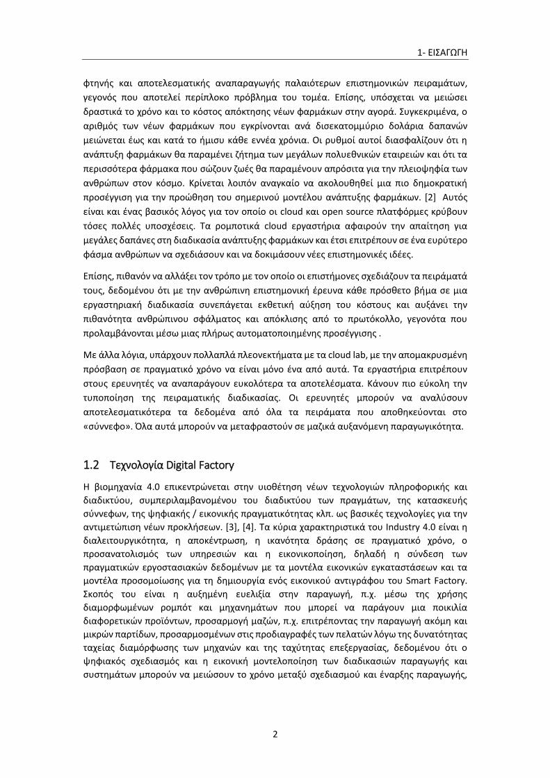
1- ΕΙΣΑΓΩΓΗ
2
φτηνής και αποτελεσματικής αναπαραγωγής παλαιότερων επιστημονικών πειραμάτων,
γεγονός που αποτελεί περίπλοκο πρόβλημα του τομέα. Επίσης, υπόσχεται να μειώσει
δραστικά το χρόνο και το κόστος απόκτησης νέων φαρμάκων στην αγορά. Συγκεκριμένα, ο
αριθμός των νέων φαρμάκων που εγκρίνονται ανά δισεκατομμύριο δολάρια δαπανών
μειώνεται έως και κατά το ήμισυ κάθε εννέα χρόνια. Οι ρυθμοί αυτοί διασφαλίζουν ότι η
ανάπτυξη φαρμάκων θα παραμένει ζήτημα των μεγάλων πολυεθνικών εταιρειών και ότι τα
περισσότερα φάρμακα που σώζουν ζωές θα παραμένουν απρόσιτα για την πλειοψηφία των
ανθρώπων στον κόσμο. Κρίνεται λοιπόν αναγκαίο να ακολουθηθεί μια πιο δημοκρατική
προσέγγιση για την προώθηση του σημερινού μοντέλου ανάπτυξης φαρμάκων. [2] Αυτός
είναι και ένας βασικός λόγος για τον οποίο οι cloud και open source πλατφόρμες κρύβουν
τόσες πολλές υποσχέσεις. Τα ρομποτικά cloud εργαστήρια αφαιρούν την απαίτηση για
μεγάλες δαπάνες στη διαδικασία ανάπτυξης φαρμάκων και έτσι επιτρέπουν σε ένα ευρύτερο
φάσμα ανθρώπων να σχεδιάσουν και να δοκιμάσουν νέες επιστημονικές ιδέες.
Επίσης, πιθανόν να αλλάξει τον τρόπο με τον οποίο οι επιστήμονες σχεδιάζουν τα πειράματά
τους, δεδομένου ότι με την ανθρώπινη επιστημονική έρευνα κάθε πρόσθετο βήμα σε μια
εργαστηριακή διαδικασία συνεπάγεται εκθετική αύξηση του κόστους και αυξάνει την
πιθανότητα ανθρώπινου σφάλματος και απόκλισης από το πρωτόκολλο, γεγονότα που
προλαμβάνονται μέσω μιας πλήρως αυτοματοποιημένης προσέγγισης .
Με άλλα λόγια, υπάρχουν πολλαπλά πλεονεκτήματα με τα cloud lab, με την απομακρυσμένη
πρόσβαση σε πραγματικό χρόνο να είναι μόνο ένα από αυτά. Τα εργαστήρια επιτρέπουν
στους ερευνητές να αναπαράγουν ευκολότερα τα αποτελέσματα. Κάνουν πιο εύκολη την
τυποποίηση της πειραματικής διαδικασίας. Οι ερευνητές μπορούν να αναλύσουν
αποτελεσματικότερα τα δεδομένα από όλα τα πειράματα που αποθηκεύονται στο
«σύννεφο». Όλα αυτά μπορούν να μεταφραστούν σε μαζικά αυξανόμενη παραγωγικότητα.
1.2 Τεχνολογία Digital Factory
Η βιομηχανία 4.0 επικεντρώνεται στην υιοθέτηση νέων τεχνολογιών πληροφορικής και
διαδικτύου, συμπεριλαμβανομένου του διαδικτύου των πραγμάτων, της κατασκευής
σύννεφων, της ψηφιακής / εικονικής πραγματικότητας κλπ. ως βασικές τεχνολογίες για την
αντιμετώπιση νέων προκλήσεων. [3], [4]. Τα κύρια χαρακτηριστικά του Industry 4.0 είναι η
διαλειτουργικότητα, η αποκέντρωση, η ικανότητα δράσης σε πραγματικό χρόνο, ο
προσανατολισμός των υπηρεσιών και η εικονικοποίηση, δηλαδή η σύνδεση των
πραγματικών εργοστασιακών δεδομένων με τα μοντέλα εικονικών εγκαταστάσεων και τα
μοντέλα προσομοίωσης για τη δημιουργία ενός εικονικού αντιγράφου του Smart Factory.
Σκοπός του είναι η αυξημένη ευελιξία στην παραγωγή, π.χ. μέσω της χρήσης
διαμορφωμένων ρομπότ και μηχανημάτων που μπορεί να παράγουν μια ποικιλία
διαφορετικών προϊόντων, προσαρμογή μαζών, π.χ. επιτρέποντας την παραγωγή ακόμη και
μικρών παρτίδων, προσαρμοσμένων στις προδιαγραφές των πελατών λόγω της δυνατότητας
ταχείας διαμόρφωσης των μηχανών και της ταχύτητας επεξεργασίας, δεδομένου ότι ο
ψηφιακός σχεδιασμός και η εικονική μοντελοποίηση των διαδικασιών παραγωγής και
συστημάτων μπορούν να μειώσουν το χρόνο μεταξύ σχεδιασμού και έναρξης παραγωγής,

1- ΕΙΣΑΓΩΓΗ
3
που απαιτούνται για την παράδοση των παραγγελιών και το χρόνο για να τεθούν τα προϊόντα
στην αγορά. [5]
Συνεπώς, η τέταρτη βιομηχανική επανάσταση δεν αντιπροσωπεύεται μόνο από την
αλληλεπίδραση μεταξύ μηχανών, ρομπότ, ηλεκτρονικών υπολογιστών και δεδομένων μέσω
του Διαδικτύου, αλλά και από την αυξημένη χρήση ψηφιακών μέσων παραγωγής και
λογισμικού, επιτρέποντας την ψηφιακή αναπαράσταση του πραγματικού περιβάλλοντος
παραγωγής, όλα τα επίπεδα από το σύνολο του εργοστασίου παραγωγής, από ένα μόνο
μηχάνημα, από μια συγκεκριμένη διαδικασία ή από μια επιχείρηση ή από τον σχεδιασμό και
την ανάπτυξη νέων προϊόντων. [6] Σε αυτό το πλαίσιο, οι τεχνολογίες Digital Factory
βασίζονται στην αξιοποίηση ψηφιακών μεθόδων και εργαλείων, όπως η αριθμητική
προσομοίωση, η τρισδιάστατη μοντελοποίηση και η εικονική πραγματικότητα για την
εξέταση ενός σύνθετου κατασκευαστικού συστήματος και την αξιολόγηση διαφορετικών
διαμορφώσεων για βέλτιστη λήψη αποφάσεων με σχετικά χαμηλό κόστος. [4], [7] Οι
τεχνολογίες που βασίζονται στην προσομοίωση είναι κεντρικά στοιχεία στην προσέγγιση
Digital Factory, καθώς επιτρέπουν τον πειραματισμό και την επικύρωση διαφόρων
διαμορφώσεων συστημάτων προϊόντων, διαδικασιών και κατασκευών. [8]
Τα κοινά ψηφιακά δεδομένα και μοντέλα στο Smart Factory θα πρέπει να είναι
προσαρμοσμένα, με την έννοια ότι πρέπει πάντα να αντιπροσωπεύουν την τρέχουσα
κατάσταση του φυσικού συστήματος παραγωγής. Για το λόγο αυτό, θα πρέπει να
ενημερώνονται τακτικά με πληροφορίες που προέρχονται από το φυσικό σύστημα
παραγωγής καθώς και με βάση τις εισόδους των χρηστών. Δεδομένου ότι τα μοντέλα είναι
ενημερωμένα και έγκυρα, μπορούν να χρησιμοποιηθούν αποτελεσματικά για τη λήψη
αποφάσεων μέσω της χρήσης έγκυρων μεθόδων βελτιστοποίησης. Ως εκ τούτου, ένα
θεμελιώδες ζήτημα αποτελεί η προσαρμογή των κοινών δεδομένων και των μοντέλων που
πραγματοποιούν μια στενή σύνδεση μεταξύ του φυσικού και του ψηφιακού κόσμου [4].
Από την άποψη αυτή, είναι εμφανής η σημασία της ανάπτυξης μεθόδων παραγωγής αιχμής
για φαρμακευτικά προϊόντα που χρησιμοποιούν τεχνολογίες ψηφιακού εργοστασίου. Τις
νεοφυείς εταιρίες, μεταξύ άλλων, μπορεί να βοηθήσει η ανάπτυξη αυτών των τεχνολογιών,
δεδομένου ότι το κόστος και ο κίνδυνος για την κατασκευή, στην περίπτωσή μας, ενός
βιοτεχνολογικού εργαστηρίου, ελαχιστοποιούνται χάρη στις τεχνολογίες προσομοίωσης,
στις οποίες η τρέχουσα εργασία βασίζεται επίσης σε μεγάλο βαθμό.
1.3 Προσπάθειες για την ανάπτυξη αυτοματοποιημένων εργαστηρίων
βιοτεχνολογίας
Οι περισσότερες εταιρείες φαρμακευτικών και βιοτεχνολογικών προϊόντων, και εν μέρει και
ακαδημαϊκά εργαστήρια, διαθέτουν αυτοματοποιημένα τμήματα των διαδικασιών τους και
χρησιμοποιούν συστήματα διαχείρισης υγρών, ενώ οι πρώτες εργαστηριακές εφαρμογές API
είναι διαθέσιμες. Οι εταιρείες Science-As-a-Service (SciAAS) άρχισαν να εμφανίζονται, με
πρόθεση να επιταχύνουν την επιστημονική έρευνα και τη βελτίωση της βιοτεχνολογίας.
Επιτρέποντας στους ερευνητές να αναθέτουν το ακριβό έργο της διεξαγωγής πειραμάτων σε
εξωτερικούς συνεργάτες, οι ομάδες εξοικονομούν χρόνο και χρήματα χωρίς να διακυβεύουν
την ποιότητα της επιστημονικής έρευνας, μειώνοντας έτσι τα εμπόδια που εμφανίζονται
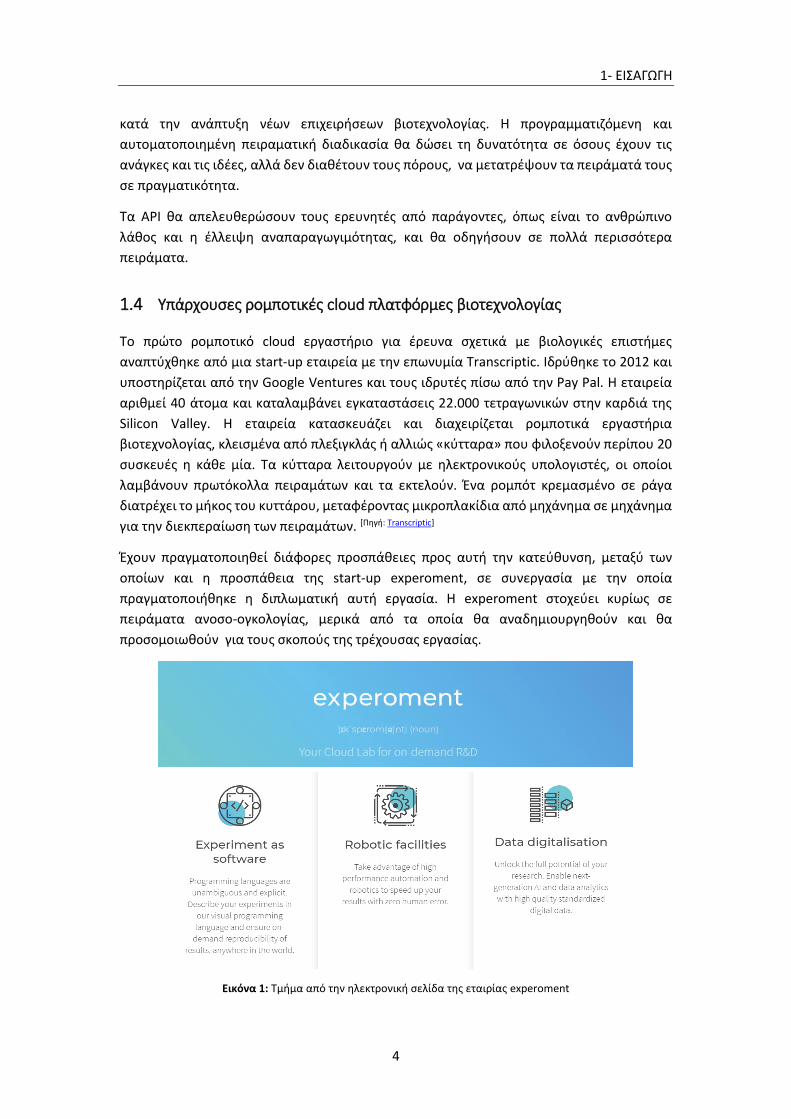
1- ΕΙΣΑΓΩΓΗ
4
κατά την ανάπτυξη νέων επιχειρήσεων βιοτεχνολογίας. Η προγραμματιζόμενη και
αυτοματοποιημένη πειραματική διαδικασία θα δώσει τη δυνατότητα σε όσους έχουν τις
ανάγκες και τις ιδέες, αλλά δεν διαθέτουν τους πόρους, να μετατρέψουν τα πειράματά τους
σε πραγματικότητα.
Τα API θα απελευθερώσουν τους ερευνητές από παράγοντες, όπως είναι το ανθρώπινο
λάθος και η έλλειψη αναπαραγωγιμότητας, και θα οδηγήσουν σε πολλά περισσότερα
πειράματα.
1.4 Υπάρχουσες ρομποτικές cloud πλατφόρμες βιοτεχνολογίας
Το πρώτο ρομποτικό cloud εργαστήριο για έρευνα σχετικά με βιολογικές επιστήμες
αναπτύχθηκε από μια start-up εταιρεία με την επωνυμία Transcriptic. Ιδρύθηκε το 2012 και
υποστηρίζεται από την Google Ventures και τους ιδρυτές πίσω από την Pay Pal. Η εταιρεία
αριθμεί 40 άτομα και καταλαμβάνει εγκαταστάσεις 22.000 τετραγωνικών στην καρδιά της
Silicon Valley. Η εταιρεία κατασκευάζει και διαχειρίζεται ρομποτικά εργαστήρια
βιοτεχνολογίας, κλεισμένα από πλεξιγκλάς ή αλλιώς «κύτταρα» που φιλοξενούν περίπου 20
συσκευές η κάθε μία. Τα κύτταρα λειτουργούν με ηλεκτρονικούς υπολογιστές, οι οποίοι
λαμβάνουν πρωτόκολλα πειραμάτων και τα εκτελούν. Ένα ρομπότ κρεμασμένο σε ράγα
διατρέχει το μήκος του κυττάρου, μεταφέροντας μικροπλακίδια από μηχάνημα σε μηχάνημα
για την διεκπεραίωση των πειραμάτων. [Πηγή: Transcriptic]
Έχουν πραγματοποιηθεί διάφορες προσπάθειες προς αυτή την κατεύθυνση, μεταξύ των
οποίων και η προσπάθεια της start-up experoment, σε συνεργασία με την οποία
πραγματοποιήθηκε η διπλωματική αυτή εργασία. Η experoment στοχεύει κυρίως σε
πειράματα ανοσο-ογκολογίας, μερικά από τα οποία θα αναδημιουργηθούν και θα
προσομοιωθούν για τους σκοπούς της τρέχουσας εργασίας.
Εικόνα 1: Τμήμα από την ηλεκτρονική σελίδα της εταιρίας experoment
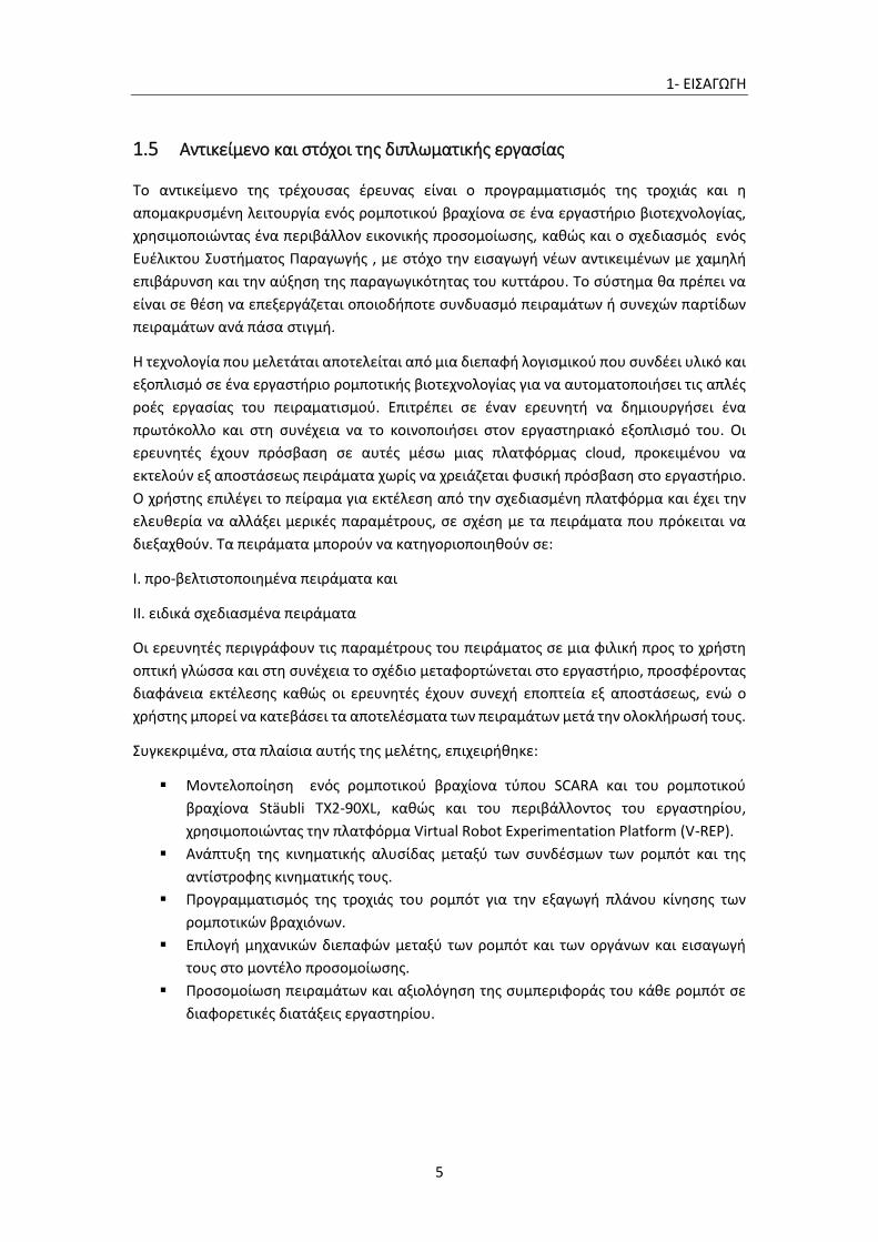
1- ΕΙΣΑΓΩΓΗ
5
1.5 Αντικείμενο και στόχοι της διπλωματικής εργασίας
Το αντικείμενο της τρέχουσας έρευνας είναι ο προγραμματισμός της τροχιάς και η
απομακρυσμένη λειτουργία ενός ρομποτικού βραχίονα σε ένα εργαστήριο βιοτεχνολογίας,
χρησιμοποιώντας ένα περιβάλλον εικονικής προσομοίωσης, καθώς και ο σχεδιασμός ενός
Ευέλικτου Συστήματος Παραγωγής , με στόχο την εισαγωγή νέων αντικειμένων με χαμηλή
επιβάρυνση και την αύξηση της παραγωγικότητας του κυττάρου. Το σύστημα θα πρέπει να
είναι σε θέση να επεξεργάζεται οποιοδήποτε συνδυασμό πειραμάτων ή συνεχών παρτίδων
πειραμάτων ανά πάσα στιγμή.
Η τεχνολογία που μελετάται αποτελείται από μια διεπαφή λογισμικού που συνδέει υλικό και
εξοπλισμό σε ένα εργαστήριο ρομποτικής βιοτεχνολογίας για να αυτοματοποιήσει τις απλές
ροές εργασίας του πειραματισμού. Επιτρέπει σε έναν ερευνητή να δημιουργήσει ένα
πρωτόκολλο και στη συνέχεια να το κοινοποιήσει στον εργαστηριακό εξοπλισμό του. Οι
ερευνητές έχουν πρόσβαση σε αυτές μέσω μιας πλατφόρμας cloud, προκειμένου να
εκτελούν εξ αποστάσεως πειράματα χωρίς να χρειάζεται φυσική πρόσβαση στο εργαστήριο.
Ο χρήστης επιλέγει το πείραμα για εκτέλεση από την σχεδιασμένη πλατφόρμα και έχει την
ελευθερία να αλλάξει μερικές παραμέτρους, σε σχέση με τα πειράματα που πρόκειται να
διεξαχθούν. Τα πειράματα μπορούν να κατηγοριοποιηθούν σε:
I. προ-βελτιστοποιημένα πειράματα και
ΙΙ. ειδικά σχεδιασμένα πειράματα
Οι ερευνητές περιγράφουν τις παραμέτρους του πειράματος σε μια φιλική προς το χρήστη
οπτική γλώσσα και στη συνέχεια το σχέδιο μεταφορτώνεται στο εργαστήριο, προσφέροντας
διαφάνεια εκτέλεσης καθώς οι ερευνητές έχουν συνεχή εποπτεία εξ αποστάσεως, ενώ ο
χρήστης μπορεί να κατεβάσει τα αποτελέσματα των πειραμάτων μετά την ολοκλήρωσή τους.
Συγκεκριμένα, στα πλαίσια αυτής της μελέτης, επιχειρήθηκε:
Μοντελοποίηση ενός ρομποτικού βραχίονα τύπου SCARA και του ρομποτικού
βραχίονα Stäubli TX2-90XL, καθώς και του περιβάλλοντος του εργαστηρίου,
χρησιμοποιώντας την πλατφόρμα Virtual Robot Experimentation Platform (V-REP).
Ανάπτυξη της κινηματικής αλυσίδας μεταξύ των συνδέσμων των ρομπότ και της
αντίστροφης κινηματικής τους.
Προγραμματισμός της τροχιάς του ρομπότ για την εξαγωγή πλάνου κίνησης των
ρομποτικών βραχιόνων.
Επιλογή μηχανικών διεπαφών μεταξύ των ρομπότ και των οργάνων και εισαγωγή
τους στο μοντέλο προσομοίωσης.
Προσομοίωση πειραμάτων και αξιολόγηση της συμπεριφοράς του κάθε ρομπότ σε
διαφορετικές διατάξεις εργαστηρίου.

1- ΕΙΣΑΓΩΓΗ
6
Οι στόχοι της παραπάνω μελέτης είναι:
Απλοποίηση της διαδικασίας προγραμματισμού τροχιάς του ρομπότ, αν ο χειριστής
ελέγχει το σημείο τερματισμού και οι τιμές των γωνιών άρθρωσης προέρχονται από
την αντίστροφη κινηματική.
Μείωση των σφαλμάτων στη φυσική παραγωγή, καθώς τα σφάλματα σε ένα εικονικό
περιβάλλον δεν έχουν φυσικές συνέπειες και μπορούν να διορθωθούν,
εξοικονομώντας χρόνο και αποτρέποντας ζημιές στη μηχανή ή δαπανηρές αποτυχίες
κατά τη διάρκεια της παραγωγής.
Ικανότητα παρακολούθησης και τροποποίησης της λειτουργίας του ρομποτικού
βραχίονα χωρίς να απαιτείται άτομο στο χώρο του εργαστηρίου. Το τελευταίο
εξαλείφει τη δυνατότητα τραυματισμού του ανθρώπινου παράγοντα με τη
μετακίνηση εξαρτημάτων.
Προσφορά μιας εναλλακτικής λύσης χαμηλού κόστους στον οπτικό έλεχγο (visual
servoing) του ρομπότ ή σε ακριβό ρομπότ υψηλής ακρίβειας, ειδικά επειδή στην
περίπτωση αυτή όλα τα αναλώσιμα στοιχεία μετακινούνται μεταξύ γνωστών
προκαθορισμένων θέσεων και προσανατολισμών και ο ρομποτικός βραχίονας είναι
υπεύθυνος για τη μεταφορά αντικειμένων προκαθορισμένων διαστάσεων από ένα
σταθμό εργασίας σε άλλο.

2- ΠΡΟΣΟΜΟΙΩΣΗ
7
2 ΠΡΟΣΟΜΟΙΩΣΗ
2.1 Ψηφιακό Μοντέλο Προσομοίωσης
Ο σημαντικότερος παράγοντας της προσομοίωσης που έχει υπογραμμιστεί καθ’ όλη τη
διάρκεια της τρέχουσας εργασίας, είναι η παροχή ευελιξίας στον ερευνητή και η
παραμετροποίηση της πειραματικής διαδικασίας, κατά τρόπο τέτοιο ώστε να μπορεί να
ολοκληρωθεί οποιοδήποτε πρωτόκολλο πειράματος, ανεξάρτητα από τον αριθμό ή τον τύπο
μηχανών, τη σειρά της χρήση τους κατά τη διάρκεια ενός πειράματος ή ακόμα και
ανεξάρτητα από τις γνώσεις του χρήστη σχετικά με ρομποτικά συστήματα.
2.1.1 Ρομπότ
Μετά την έκφραση της κινηματικής αλυσίδας κάθε ρομπότ ως αρχείο URDF, τα μοντέλα
εισάγονται στη σκηνή προσομοίωσης. Κάθε ρομπότ αποτελείται από δικούς του συνδέσμους
και αρθρώσεις, ενώ στα αρχεία URDF προστέθηκαν δύο επιπλέον οντότητες, συγκεκριμένα
τα ee_link και world.
Ο ρόλος του world, που θα αναφέρεται ως world frame του ρομπότ και δεν πρέπει να
συγχέεται με το global frame του VREP, είναι να παράσχει ένα σημείο αναφοράς για όλα όσα
συμβαίνουν στη σκηνή προσομοίωσης. Δεδομένου ότι οι ρομποτικοί βραχίονες αποτελούν
το κεντρικό θέμα της λειτουργίας των ρομποτικών συστημάτων, είναι λογικό να εκφράζονται
ως προς το world frame, όχι μόνο η θέση και ο προσανατολισμός των συνδέσμων και των
αρθρώσεων του ρομπότ, αλλά και η θέση και ο προσανατολισμός όλων των συνιστωσών μιας
σκηνής.
Αντίστοιχα, το ee_link αντιπροσωπεύει την πραγματική τελική θέση του τελικού σημείου
δράσης, η οποία είναι πάντα περίπου στη μέση της αρπάγης, αντιπροσωπεύοντας το σημείο
όπου θα προσαρτηθεί το μικροπλακίδιο. Ωστόσο, είναι πιθανό το ee_link του αρχείου URDF
να μην συμπίπτει με το πραγματικό σημείο πιασίματος, αλλά να συμπίπτει μονάχα με τη
βάση της αρπάγης ή την τελική άρθρωση ενός ρομπότ. Σε αυτή την περίπτωση, ένα
ee_link_dummy προστίθεται στη σκηνή VREP. Το ee_link_dummy εκφράζεται στη συνέχεια
σε σχέση με το ee_link του URDF, μέσω ενός κατάλληλου offset και αυτό αργότερα
εκφράζεται σε σχέση με τον κόσμο. Η διατήρηση της ομοιογενούς έκφρασης της θέσης και
του προσανατολισμού ως προς ένα σημείο αναφοράς είναι το κλειδί για μια επιτυχημένη και
με ακρίβεια προσομοίωση.

2- ΠΡΟΣΟΜΟΙΩΣΗ
8
Εικόνα 2: Το ee_link_dummy για την περίπτωση του SCARA (πάνω) και του STAUBLI (κάτω)
2.1.2 Εργαστηριακός Εξοπλισμός
Ο εργαστηριακός εξοπλισμός, συμπεριλαμβανομένων των μηχανών και των αναλώσιμων
εισάγονται στη σκηνή σύμφωνα με την επιθυμητή διάταξη. Ο στόχος είναι να δημιουργηθεί
ένα περιβάλλον όπου το ρομπότ θα μπορεί να εντοπίζει τα σημεία φόρτωσης και
εκφόρτωσης κάθε μηχανής σε σχέση με το world frame του, όπως αυτό αναλύθηκε
προηγουμένως. Προκειμένου το ρομπότ να καταλάβει ποια μηχανήματα θα πρέπει να
επισκεφθεί κατά τη διάρκεια ενός πειράματος, dummies από το VREP τοποθετούνται στις
θέσεις φόρτωσης-εκφόρτωσης κάθε μηχανής και ονομάζονται με βάση την ονομασία της
μηχανής στην οποία ανήκουν. Είναι σημαντικό ο προσανατολισμός των dummies να είναι ο
ίδιος με τον προσανατολισμό του ee_link_dummy στο τελικό σημείο δράσης, έτσι ώστε ο
ρομποτικός βραχίονας να μπορεί να προσεγγίσει τη σωστή θέση με τον σωστό
προσανατολισμό. Οι θέσεις των μηχανών και του περιβάλλοντος του εργαστηρίου όπου οι
ρομποτικοί βραχίονες πρέπει να φορτώνουν και να εκφορτώνουν τα μικροπλακίδια
παρουσιάζονται στην Εικόνα 3.

2- ΠΡΟΣΟΜΟΙΩΣΗ
9
Εικόνα 3: Σημεία φόρτωσης-εκφόρτωσης των εργαστηριακών μηχανών
2.1.3 Ασφαλείς Θέσεις
Τα dummies δεν χρησιμοποιούνται μόνο για να εκφράσουν τη θέση και τον προσανατολισμό
ενός αντικειμένου σε σχέση με το world frame του ρομπότ, αλλά χρησιμοποιούνται επίσης
ως σημεία αναφοράς για να περιγράψουν κάποιες άλλες θέσεις στον χώρο, οι οποίες είναι
απαραίτητες για την πραγματοποίηση ομαλής τροχιάς του ρομπότ.
Για παράδειγμα, συνιστάται ιδιαίτερα να χρησιμοποιούνται ενδιάμεσα σημεία μεταξύ της
αρχικής θέσης ρομπότ και οποιασδήποτε θέσης μηχανής. Ο καθορισμός μιας ασφαλούς
θέσης μηχανής βοηθά στην εξάλειψη των συγκρούσεων του ρομπότ με τον εργαστηριακό
εξοπλισμό. Μια τέτοια θέση μηχανής μπορεί να οριστεί ως η θέση μηχανής +/- μια
μετατόπιση. Η μετατόπιση μπορεί να αντιπροσωπεύει μια απόσταση από την πραγματική
θέση φόρτωσης-εκφόρτωσης που θεωρείται ασφαλής για να προσεγγίσει το ρομπότ, πριν
ολοκληρώσει την κίνησή του.
Οι ασφαλείς θέσεις στα πειράματα που ακολουθούνται καθορίζονται για τις ακόλουθες
περιπτώσεις:
Πριν ο ρομποτικός βραχίονας SCARA πλησιάσει την περιστροφική βάση στην οποία
αλλάζουν οι προσανατολισμοί των μικροπλακών για να αποφευχθεί η σύγκρουση με
τα μηχανήματα κατά την αναδίπλωση / ξεδίπλωση του βραχίονα
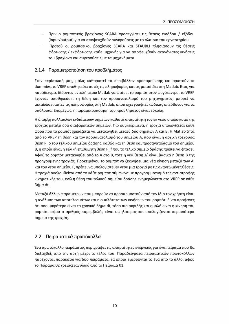
2- ΠΡΟΣΟΜΟΙΩΣΗ
10
Πριν ο ρομποτικός βραχίονας SCARA προσεγγίσει τις θέσεις εισόδου / εξόδου
(input/output) για να αποφευχθούν συγκρούσεις με το πλαίσιο του εργαστηρίου
Προτού οι ρομποτικοί βραχίονες SCARA και STAUBLI πλησιάσουν τις θέσεις
φόρτωσης / εκφόρτωσης κάθε μηχανής για να αποφευχθούν ακανόνιστες κινήσεις
του βραχίονα και συγκρούσεις με τα μηχανήματα
2.1.4 Παραμετροποίηση του προβλήματος
Στην περίπτωσή μας, μόλις καθοριστεί το περιβάλλον προσομοίωσης και οριστούν τα
dummies, το VREP αποθηκεύει αυτές τις πληροφορίες και τις μεταδίδει στη Matlab. Έτσι, για
παράδειγμα, δίδοντας εντολή μέσω Matlab να φτάσει το ρομπότ στον φυγόκεντρο, το VREP
έχοντας αποθηκεύσει τη θέση και τον προσανατολισμό του μηχανήματος, μπορεί να
μεταδώσει αυτές τις πληροφορίες στη Matlab, όπου έχει γραφτεί κώδικας υπεύθυνος για τα
υπόλοιπα. Επομένως, η παραμετροποίηση του προβλήματος είναι εύκολη.
Η ύπαρξη πολλαπλών ενδιάμεσων σημείων καθιστά απαραίτητη τον εκ νέου υπολογισμό της
τροχιάς μεταξύ δύο διαφορετικών σημείων. Πιο συγκεκριμένα, η τροχιά υπολογίζεται κάθε
φορά που το ρομπότ χρειάζεται να μετακινηθεί μεταξύ δύο σημείων Α και Β. Η Matlab ζητά
από το VREP τη θέση και τον προσανατολισμό του σημείου Α, που είναι η αρχική τρέχουσα
θέση P_o του τελικού σημείου δράσης, καθώς και τη θέση και προσανατολισμό του σημείου
Β, η οποία είναι η τελική επιθυμητή θέση Ρ_f που το τελικό σημείο δράσης πρέπει να φτάσει.
Αφού το ρομπότ μετακινηθεί από το Α στο Β, τότε η νέα θέση Α’ είναι βασικά η θέση Β της
προηγούμενης τροχιάς. Προκειμένου το ρομπότ να ξεκινήσει μια νέα κίνηση μεταξύ των Α’
και του νέου σημείου Γ, πρέπει να υπολογιστεί εκ νέου μια τροχιά με τις ανανεωμένες θέσεις.
Η τροχιά ακολουθείται από το κάθε ρομπότ σύμφωνα με προγραμματισμό της αντίστροφης
κινηματικής του, ενώ η θέση του τελικού σημείου δράσης ενημερώνεται στο VREP σε κάθε
βήμα dt.
Μεταξύ άλλων παραμέτρων που μπορούν να προσαρμοστούν από τον ίδιο τον χρήστη είναι
η ανάλυση των αποτελεσμάτων και η ομαλότητα των κινήσεων του ρομπότ. Είναι προφανές
ότι όσο μικρότερο είναι το χρονικό βήμα dt, τόσο πιο ακριβής και ομαλή είναι η κίνηση του
ρομπότ, αφού ο αριθμός παρεμβολής είναι υψηλότερος και υπολογίζονται περισσότερα
σημεία της τροχιάς.
2.2 Πειραματικά πρωτόκολλα
Ένα πρωτόκολλο πειράματος περιγράφει τις απαραίτητες ενέργειες για ένα πείραμα που θα
διεξαχθεί, από την αρχή μέχρι το τέλος του. Παραδείγματα πειραματικών πρωτοκόλλων
παρέχονται παρακάτω για δύο πειράματα, τα οποία εξαρτώνται το ένα από το άλλο, αφού
το Πείραμα 02 χρειάζεται υλικό από το Πείραμα 01.

2- ΠΡΟΣΟΜΟΙΩΣΗ
11
Εικόνα 4: Παραδείγματα πειραματικών πρωτοκόλλων
2.3 Διεπαφή χρήστη-ρομπότ
Η διευκόλυνση της επικοινωνίας μεταξύ του χρήστη (ερευνητή) και του περιβάλλοντος
προσομοίωσης έχει μεγάλη σημασία, καθώς η πλατφόρμα πρέπει να είναι προσβάσιμη σε
ανθρώπους που δεν έχουν βαθιά γνώση ρομποτικής. Ο στόχος είναι απλά ο χρήστης να είναι
σε θέση να επικοινωνήσει στο ρομποτικό σύστημα ένα πρωτόκολλο πειράματος όπως
παρουσιάστηκε παραπάνω, με την ελάχιστη δυνατή προσπάθεια. Για αυτό το σκοπό σκόπιμη
κρίνεται η δημιουργία μιας διεπιφάνειας φιλικής προς τον χρήστη.
KEY

2- ΠΡΟΣΟΜΟΙΩΣΗ
12
Με την έναρξη των προγραμμάτων main_SCARA.m και main_STAUBLI.m, τα οποία είναι
τα δύο προγράμματα Matlab υπεύθυνα για όλα όσα συμβαίνουν σε κάθε εργαστήριο, ο
χρήστης καλείται να εισάγει σταθμούς εργασίας στο κύτταρο:
Input working station:
Σε αυτό το σημείο, ο χρήστης μπορεί να εισάγει το όνομα των σταθμών εργασίας -
εργαστηριακές μηχανές - που περιλαμβάνονται στο πείραμα και με τη σειρά που ο χρήστης
επιθυμεί να χρησιμοποιηθεί κάθε μηχανή, μαζί με το χρόνο που ο χρήστης επιθυμεί για το
κάθε δείγμα να παραμένει σε κάθε μηχάνημα. Κάθε μηχανή μπορεί να χρησιμοποιηθεί
περισσότερες από μία φορές, εάν το πείραμα απαιτεί την επίσκεψη συγκεκριμένου σταθμού
εργασίας πολλαπλές φορές. Αφού συμπεριληφθούν όλες οι μηχανές και οι αντίστοιχοι
χρόνοι με τη σωστή σειρά, ο χρήστης μπορεί να πληκτρολογήσει stop για να υποδείξει ότι
το πρωτόκολλο πειράματος είναι πλήρες και ότι όλος ο απαραίτητος εξοπλισμός έχει ήδη
αναφερθεί.
Για τις ανάγκες της τρέχουσας μελέτης, οι χρόνοι δεν έχουν ληφθεί υπόψη, αφού μπορούν
να φτάσουν ακόμα και σε δύο ημέρες αναμονής σε μια συγκεκριμένη μηχανή. Έτσι, αυτή η
διαδικασία αντιπροσωπεύεται από τη διακοπή των κινήσεων βραχίονα για μερικά
δευτερόλεπτα.
Αφού εισαχθεί το πρωτόκολλο στην πλατφόρμα, το πρόγραμμα ελέγχει αν το ρομπότ
βρίσκεται στην αρχική του θέση, η οποία είναι μια ασφαλής θέση για το ρομπότ να ξεκινήσει
οποιοδήποτε πείραμα. Εάν υπάρχει, ο χρήστης θα σας ζητήσει την ειδοποίηση:
Robot is in Home Position-Ready to start experiment
Διαφορετικά, το ρομπότ μετακινείται στην αρχική του θέση και στη συνέχεια ο χρήστης
καλείται για τελευταία φορά αν επιθυμεί να προχωρήσει με το πείραμα. Η προεπιλεγμένη
απάντηση είναι ΝΑΙ.
Do you wish to continue to experiment? Y/N [Y]:
Εάν ο χρήστης πληκτρολογήσει N, τότε το πείραμα διακόπτεται. Εάν ο χρήστης
πληκτρολογήσει Y, το πείραμα ξεκινά σύμφωνα με το πρωτόκολλό του.
Εάν ο χρήστης έχει κάποια γνώση σχετικά με τη ρομποτική, μπορεί επίσης να τροποποιήσει
το χρόνο T και το βήμα dt που χρησιμοποιείται για τον προγραμματισμό της τροχιάς και την
κίνηση των όπλων.
Παρακάτω παρέχεται ένα διάγραμμα ροής, το οποίο αντιπροσωπεύει την αλληλεπίδραση
του χρήστη με την πλατφόρμα.

2- ΠΡΟΣΟΜΟΙΩΣΗ
13
Εικόνα 5: Διαγραμματική απεικόνιση διεπαφής χρήστη- περιβάλλοντος εργασίας
2.4 Προσομοίωση πειραμάτων με τους ρομποτικούς βραχίονες SCARA και
STAUBLI
Μετά την έναρξη του πειράματος, το ρομπότ αποκτά διαφορετικές θέσεις και διαμορφώσεις
στο διάστημα, οι οποίες εξαρτώνται από τον τελικό του προορισμό και τους περιορισμούς
που επιβάλλονται. Παρακάτω παρουσιάζεται μια σειρά εικόνων που δείχνουν αυτές τις
πληροφορίες τόσο για το ρομπότ SCARA όσο και για το STAUBLI.
2.4.1 SCARA
Εικόνα 6: Αρχική θέση του ρομπότ SCARA
Εικόνα 7: Το ρομπότ SCARA παίρνει το
μικροπλακίδιο από τον τεχνικό του εργαστηρίου (θέση input)

2- ΠΡΟΣΟΜΟΙΩΣΗ
14
Εικόνα 9: Ασφαλής απόσταση SCARA από
εξοπλισμό εργαστηρίου
Εικόνα 10: Η αρπάγη του SCARA είναι έτοιμη να
αφήσει/παραλάβει πλακίδιο
Εικόνα 11: Ρομπότ SCARA επιστρέφει
μικροπλακίδιο σε τεχνικό εργαστηρίου (θέση output)
Εικόνα 12: Επιστροφή SCARA σε αρχική θέση
Εικόνα 8: Μετακίνηση ρομπότ SCARA πάνω από μικροπλακίδιο σε περιστρεφόμενη

2- ΠΡΟΣΟΜΟΙΩΣΗ
15
2.4.2 STAUBLI TX2-90XL
Εικόνα 13: Αρχική θέση του ρομπότ STAUBLI Εικόνα 14: Το ρομπότ STAUBLI παίρνει το μικροπλακίδιο
από τον τεχνικό του εργαστηρίου (θέση input)
]]
Εικόνα 15: Ασφαλής απόσταση STAUBLI από εξοπλισμό εργαστηρίου
Εικόνα 16: Η αρπάγη του STAUBLI είναι έτοιμη να αφήσει/παραλάβει πλακίδιο

2- ΠΡΟΣΟΜΟΙΩΣΗ
16
Εικόνα 17: Το ρομπότ STAUBLI επιστρέφει το μικροπλακίδιο στον τεχνικό του εργαστηρίου (θέση output)
Εικόνα 18: Επιστροφή STAUBLI σε αρχική θέση

3- ΑΠΟΤΕΛΕΣΜΑΤΑ
17
3 ΑΠΟΤΕΛΕΣΜΑΤΑ
3.1 Σχολιασμός
Τα παρακάτω διαγράμματα είναι τα αποτελέσματα των προσομοιώσεων που έγιναν
σύμφωνα με τα πρωτόκολλα πειράματος που αναφέρθηκαν προηγουμένως. Μόνο οι πιο
βασικές κινήσεις κάθε ρομπότ περιλαμβάνονται σε αυτά τα διαγράμματα για λόγους
συντομίας, ωστόσο οι συμπεριφορές των ρομπότ δεν αλλάζουν σημαντικά μεταξύ των
κινήσεων. Είναι σημαντικό να σημειωθεί και να δοθεί προσοχή στην κλίμακα του άξονα κάθε
διαγράμματος. Συγκεκριμένα, σε ορισμένες περιπτώσεις τα γραφήματα μπορεί να φαίνεται
ότι αποκλίνουν ή ότι παρουσιάζουν σημαντικά σφάλματα, αλλά αυτό οφείλεται συνήθως
στην κλίμακα του άξονα του οποίου το μέγεθος μπορεί να αντιπροσωπεύει αλλαγές στο 10-3
του αντίστοιχου μεγέθους. Τα αποτελέσματα του SCARA και του STAUBLI παρουσιάζονται
χωριστά.
Για το SCARA αξίζει να σημειωθεί ότι η 5η άρθρωση, δηλαδή η άρθρωση της αρπάγης, η
οποία την περιστρέφει, έχει οριστεί ως 0 για όλες τις προσομοιώσεις που υπάρχουν. Αυτό
οφείλεται στο γεγονός ότι, δεδομένου ότι όλα τα μηχανήματα είναι στη σειρά, δεν χρειάζεται
να περιστρέφεται η λαβή. Αν αυτό είναι απαραίτητο, τότε η αντίστοιχη άρθρωση μπορεί να
«ενεργοποιηθεί» θέτοντας τα ανώτερα και κατώτερα όριά της στο πρόγραμμα
SCARAplatetraj.m. Η ίδια προσέγγιση μπορεί επίσης να χρησιμοποιηθεί για το ρομπότ
STAUBLI.
Στα αποτελέσματα των προσομοιώσεων που παρατίθενται, όλες οι αρθρώσεις του ρομπότ
είναι «ενεργοποιημένες» και λειτουργούν σύμφωνα με τα αντίστοιχα όριά τους, όπως
καθορίζονται από την εταιρεία και όπως αυτά αναφέρονται σε προηγούμενα κεφάλαια. Αν
όμως το ρομπότ συμπεριφέρεται απροσδόκητα και όχι σύμφωνα με τον επιθυμητό τρόπο,
με την έννοια ότι δεν κρατάει τα μικροπλακίδια παράλληλα προς το έδαφος, η 4η και η 6η
άρθρωση μπορούν να τεθούν ως 0, δηλαδή να μην πραγματοποιούν περιστροφικές κινήσεις.
Η τέταρτη άρθρωση ελέγχει την περιστροφή του αντιβραχίου, ενώ η έκτη ελέγχει την
περιστροφή της φλάντζας του εργαλείου. Κρατώντας αυτά τα δύο ακίνητα, τότε το πρόβλημα
μπορεί να αντιμετωπιστεί ανάλογα.
Συνολικά, τα προκύπτοντα γραφήματα είναι πολύ ικανοποιητικά, δείχνοντας ότι οι
χρησιμοποιούμενες μέθοδοι και οι αλγόριθμοι πέτυχαν τον αρχικό στόχο, που ήταν ο έλεγχος
των ρομποτικών βραχιόνων, σύμφωνα όχι μόνο με τις δικές τους αλλά και με αυτές του
περιβάλλοντός τους. Πιο συγκεκριμένα:

3- ΑΠΟΤΕΛΕΣΜΑΤΑ
18
Οι αρθρώσεις των ρομπότ παραμένουν πάντοτε εντός των προκαθορισμένων ορίων
τους και δεν τα υπερβαίνουν, όπως αντιπροσωπεύουν τα διαγράμματα των γωνιών
των αρθρώσεων «Joint angles»
Οι ταχύτητες έχουν την αναμενόμενη καμπύλη και στις δύο περιπτώσεις της
προσομοίωσης.
Το σφάλμα θέσης εξαλείφεται στις περισσότερες περιπτώσεις, εκτός από την κίνηση
Home-Plate του SCARA. Αυτό πιθανότατα συμβαίνει επειδή η πρώτη άρθρωση του
SCARA, που ευθύνεται για την κατά μήκος μετακίνηση του ρομπότ στο εργαστήριο,
είναι ανενεργή. Ταυτόχρονα, τα σημεία που τροφοδοτούνται στον ρομποτικό
βραχίονα πιθανώς να μην είναι πλήρως γραμμικά, γεγονός που καθιστά πιο δύσκολο
το να τα ακολουθήσει ο βραχίονας. Αυτός είναι και ο λόγος για τον οποίο
παρατηρούνται σφάλματα, αλλά δεν είναι αρκετά μεγάλα για να διαταράξουν το
πείραμα και να επηρεάσουν την ακρίβειά του.
Τα διαγράμματα έχουν ληφθεί για τιμές Τ=1 και dt=0,01.
3.1.1 SCARA
A. Από Αρχική θέση σε Ασφαλή θέση πριν από θέση Input μέσω ΕΚ (Ευθείας
Κινηματικής)
Διάγραμμα 34 : Θέση ΤΣΔ του SCARA με ΕΚ- Αρχική σε Ασφαλή θέση
Διάγραμμα 35: Γωνιακές ταχύτητες αρθρώσεων του SCARA με ΕΚ- Αρχική σε Ασφαλή θέση

3- ΑΠΟΤΕΛΕΣΜΑΤΑ
19
Διάγραμμα 36:Γωνίες αρθρώσεων του SCARA με ΕΚ- Αρχική σε Ασφαλή θέση
B. Από Ασφαλή θέση πριν από θέση Input σε θέση Input μέσω ΑΚ
(αντίστροφης κινηματικής )
Διάγραμμα 37: Επιθυμητή vs Πραγματική θέση ΤΣΔ του SCARA με ΑΚ- Ασφαλής σε θέση Input
Διάγραμμα 38: Γωνίες αρθρώσεων του SCARA με ΑΚ- Ασφαλής σε θέση Input
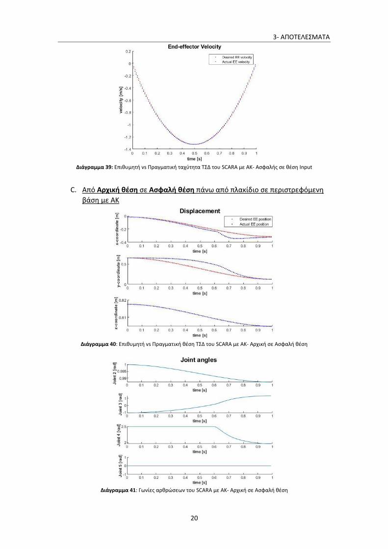
3- ΑΠΟΤΕΛΕΣΜΑΤΑ
20
Διάγραμμα 39: Επιθυμητή vs Πραγματική ταχύτητα ΤΣΔ του SCARA με ΑΚ- Ασφαλής σε θέση Input
C. Από Αρχική θέση σε Ασφαλή θέση πάνω από πλακίδιο σε περιστρεφόμενη
βάση με ΑΚ
Διάγραμμα 40: Επιθυμητή vs Πραγματική θέση ΤΣΔ του SCARA με ΑΚ- Αρχική σε Ασφαλή θέση
Διάγραμμα 41: Γωνίες αρθρώσεων του SCARA με ΑΚ- Αρχική σε Ασφαλή θέση

3- ΑΠΟΤΕΛΕΣΜΑΤΑ
21
Διάγραμμα 42: Ταχύτητα ΤΣΔ του SCARA με ΑΚ- Αρχική σε Ασφαλή θέση
D. Από Ασφαλή θέση πάνω από πλακίδιο σε Πλακίδιο σε περιστρεφόμενη
βάση με ΑΚ
Διάγραμμα 43: Επιθυμητή vs Πραγματική θέση ΤΣΔ του SCARA με ΑΚ- Ασφαλής θέση σε Πλακίδιο
Διάγραμμα 44: Γωνίες αρθρώσεων του SCARA με ΑΚ- Ασφαλής θέση σε Πλακίδιο

3- ΑΠΟΤΕΛΕΣΜΑΤΑ
22
Διάγραμμα 45: Επιθυμητή vs Πραγματική ταχύτητα ΤΣΔ του SCARA με ΑΚ- Ασφαλής θέση σε Πλακίδιο
E. Από Μηχάνημα 1 σε Μηχάνημα 2 μέσω ΑΚ
Διάγραμμα 46: Επιθυμητή vs Πραγματική θέση ΤΣΔ του SCARA με ΑΚ – Μηχάνημα 1 σε Μηχάνημα 2
Διάγραμμα 47: Γωνίες αρθρώσεων του SCARA με ΑΚ – Μηχάνημα 1 σε Μηχάνημα 2

3- ΑΠΟΤΕΛΕΣΜΑΤΑ
23
Διάγραμμα 48: Επιθυμητή vs Πραγματική ταχύτητα ΤΣΔ του SCARA με ΑΚ – Μηχάνημα 1 σε Μηχάνημα 2
F. Από Αρχική θέση σε Ασφαλή θέση πριν τη θέση Output μέσω ΕΚ
Διάγραμμα 49: Θέση ΤΣΔ του SCARA με ΕΚ- Αρχική σε Ασφαλή θέση
Διάγραμμα 50: Γωνίες αρθρώσεων SCARA με ΕΚ- Αρχική σε Ασφαλή θέση

3- ΑΠΟΤΕΛΕΣΜΑΤΑ
24
Διάγραμμα 51: Γωνιακές ταχύτητες αρθρώσεων του SCARA με ΕΚ- Αρχική σε Ασφαλή θέση
G. Από Ασφαλή θέση πριν θέση Output σε θέση Output μέσω ΑΚ
Διάγραμμα 52: Επιθυμητή vs Πραγματική θέση ΤΣΔ του SCARA με ΑΚ – Ασφαλής σε θέση Output
Διάγραμμα 53: Γωνίες αρθρώσεων SCARA με ΑΚ- Ασφαλής σε θέση Output
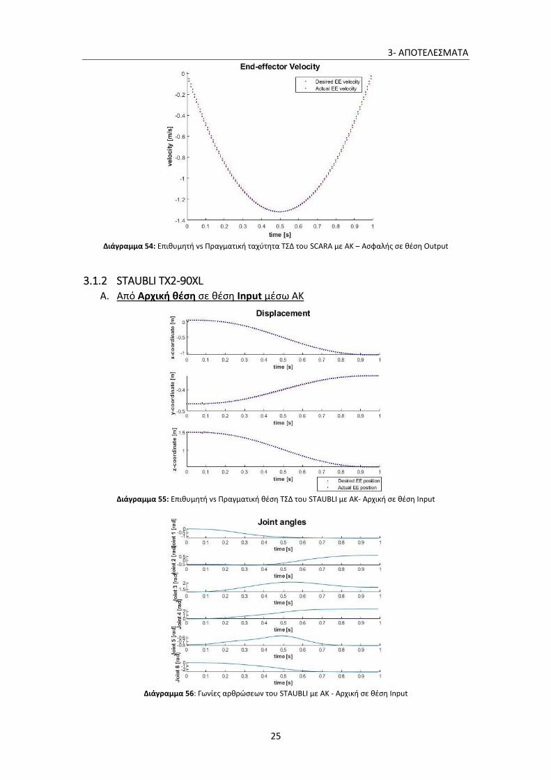
3- ΑΠΟΤΕΛΕΣΜΑΤΑ
25
Διάγραμμα 54: Επιθυμητή vs Πραγματική ταχύτητα ΤΣΔ του SCARA με ΑΚ – Ασφαλής σε θέση Output
3.1.2 STAUBLI TX2-90XL A. Από Αρχική θέση σε θέση Input μέσω ΑΚ
Διάγραμμα 55: Επιθυμητή vs Πραγματική θέση ΤΣΔ του STAUBLI με ΑΚ- Αρχική σε θέση Input
Διάγραμμα 56: Γωνίες αρθρώσεων του STAUBLI με ΑΚ - Αρχική σε θέση Input

3- ΑΠΟΤΕΛΕΣΜΑΤΑ
26
Διάγραμμα 57: Επιθυμητή vs Πραγματική ταχύτητα ΤΣΔ του STAUBLI με ΑΚ- Αρχική σε θέση Input
B. Από Αρχική θέση σε Μηχάνημα 1 με ΑΚ
Διάγραμμα 58: Επιθυμητή vs Πραγματική θέση ΤΣΔ του STAUBLI με ΑΚ – Ασφαλής θέση σε Μηχάνημα 1
Διάγραμμα 59: Γωνίες αρθρώσεων του STAUBLI με ΑΚ – Ασφαλής θέση σε Μηχάνημα 1

3- ΑΠΟΤΕΛΕΣΜΑΤΑ
27
Διάγραμμα 60: Επιθυμητή vs Πραγματική ταχύτητα ΤΣΔ του STAUBLI με ΑΚ – Ασφαλής θέση σε Μηχάνημα 1
C. Μηχάνημα 1 σε Αρχική θέση με ΕΚ
Διάγραμμα 61: Θέση ΤΣΔ του STAUBLI με ΕΚ- Μηχάνημα 1 σε Αρχική θέση
Διάγραμμα 62: Γωνίες αρθρώσεων του STAUBLI με ΕΚ- Μηχάνημα 1 σε Αρχική θέση

3- ΑΠΟΤΕΛΕΣΜΑΤΑ
28
Διάγραμμα 63: Γωνιακές ταχύτητες αρθρώσεων του STAUBLI με ΕΚ- Μηχάνημα 1 σε Αρχική θέση
D. Από Αρχική θέση σε θέση Output με ΑΚ
Διάγραμμα 64: Επιθυμητή vs Πραγματική θέση ΤΣΔ του STAUBLI με ΑΚ – Αρχική σε θέση Output
Διάγραμμα 65: Γωνίες αρθρώσεων του STAUBLI με ΑΚ – Αρχική σε θέση Output

3- ΑΠΟΤΕΛΕΣΜΑΤΑ
29
Διάγραμμα 66: Επιθυμητή vs Πραγματική ταχύτητα ΤΣΔ του STAUBLI με ΑΚ – Αρχική σε θέση Output

4- ΣΥΜΠΕΡΑΣΜΑΤΑ
30
4 ΣΥΜΠΕΡΑΣΜΑΤΑ
4.1 Συνεισφορά
Στην παρούσα εργασία αναπτύχθηκε μια μεθοδολογία ανάπτυξης του μοντέλου ενός
εργαστηριακού χώρου βιοτεχνολογίας σε περιβάλλον εικονικής πραγματικότητας. Η
διαδικασία περιλάμβανε τόσο την εισαγωγή των 3D μοντέλων για την αναπαράσταση του
φυσικού χώρου, όσο και τον προγραμματισμό τους ώστε τα ρομπότ να αποκτήσουν «ζωή»
και να αλληλεπιδρούν με τα υπόλοιπα μέρη της σκηνής.
Η κύρια συμβολή αυτής της εργασίας είναι η ανάπτυξη μεθοδολογίας για τον κινηματικό
έλεγχο δύο διαφορετικών ρομπότ και δύο διαφορετικών εργαστηριακών διατάξεων , τα
οποία μπορούν να χρησιμοποιηθούν ως εναλλακτική λύση χαμηλού κόστους στον οπτικό
έλεγχο ή στα ακριβά -υψηλής ακρίβειας- ρομπότ. Η εργασία αυτή μπορεί να αποτελέσει
υπόβαθρο για την επέκταση ή ακόμα και την ανάπτυξη άλλων σχετικών μεθοδολογιών.
Συγκεκριμένα παρέχονται:
1. Μοντέλο ενός προσαρμοσμένου στις ανάγκες της εργασίας ρομποτικού βραχίονα
τύπου SCARA με πλήρως ανεπτυγμένη κινηματική αλυσίδα μεταξύ των συνδέσμων.
2. Μοντέλο του ρομποτικού βραχίονα Stäubli TX2-90XL με πλήρως ανεπτυγμένη
κινηματική αλυσίδα μεταξύ των συνδέσμων.
3. Μοντέλο πραγματικών διαστάσεων του χώρου του εργαστηρίου βιοτεχνολογίας.
4. Ευθεία και αντίστροφη κινηματική ανάλυση των ρομποτικών βραχιόνων.
5. Προσομοίωση ολοκληρωμένων πειραματικών πρωτοκόλλων στην πλατφόρμα VREP.
4.2 Πλεονεκτήματα περιβάλλοντος εικονικής πραγματικότητας
Ο συμβατικός προγραμματισμός εργασιών ενός ρομπότ, στηριζόταν ανέκαθεν στην εμπειρία
του χειριστή, ο οποίος προγραμμάτιζε την τροχιά του ενώ βρισκόταν σε λειτουργία. Ο τρόπος
αυτός εκτός από το ότι ήταν χρονοβόρος, εγκυμονούσε τον κίνδυνο του λάθους, θέτοντας σε
κίνδυνο την ακεραιότητα του χειριστή, του βιομηχανικού εξοπλισμού καθώς και της
εργασίας.
Στη σημερινή εποχή, νέοι μηχανικοί καλούνται να εκτελέσουν την διαδικασία του
προγραμματισμού. Λόγω της εξοικείωσής τους με τις τεχνολογίες εικονικής
πραγματικότητας, η χρήση της τελευταίας στην εργασία αυτή δίνει γρήγορα, αξιόπιστα και
ασφαλή αποτελέσματα.

4- ΣΥΜΠΕΡΑΣΜΑΤΑ
31
Όφελος υπάρχει προφανώς και από οικονομικής άποψης. Χρηματικοί πόροι εξοικονομούνται
λόγω της μείωσης των απαιτούμενων εργατοωρών, των αποτυχημένων προσπαθειών καθώς
και των ζημιών που προκαλούν οι συγκρούσεις. Επίσης, ένα τέτοιο σύστημα μπορεί να
χρησιμοποιηθεί για την σωστή μελέτη τοποθέτησης πρόσθετου εξοπλισμού σε ένα ήδη
υπάρχον περιβάλλον.
4.3 Προτάσεις για μελλοντική έρευνα
Η ανάπτυξη του εργαστηρίου και ο σχεδιασμός των τροχιών ήταν επιτυχημένα, αλλά υπάρχει
ακόμα περιθώριο βελτίωσης.
Όσον αφορά στο εργαστηριακό περιβάλλον που έχει δημιουργηθεί:
Τα σενάρια του πειράματος που δοκιμάστηκαν για τους σκοπούς της παρούσας
εργασίας περιελάμβαναν μόνο 5 μηχανές - σταθμούς εργασίας μέσα στις
εργαστηριακές διατάξεις. Αυτά τα μηχανήματα είναι τα πιο συνηθισμένα που
μπορεί να υπάρξουν σε ένα εργαστήριο βιοτεχνολογίας και χρησιμοποιούνται συχνά
για τη διεξαγωγή πειραμάτων. Μια πιθανή επέκταση θα μπορούσε να είναι η
εισαγωγή πιο εξειδικευμένων μηχανών στις ίδιες εργαστηριακές εγκαταστάσεις για
την πραγματοποίηση πειραμάτων.
Στην παρούσα διπλωματική εργασία προσομοιώνεται ένα πείραμα σε κάθε τρέξιμο
του προγράμματος, γεγονός που σημαίνει ότι ένα νέο πείραμα προβλέπεται να
ξεκινήσει αμέσως μετά την ολοκλήρωση του προηγούμενου πειράματος και όχι
παράλληλα με αυτό. Μελέτη αλγορίθμων σχετικά με τον προγραμματισμό του
ευέλικτου συστήματος παραγωγής θα μπορούσε να οδηγήσει σε πραγματοποίηση
πολλαπλών πειραμάτων στο εργαστήριο ταυτόχρονα. Ενσωματώνοντας συστήματα
όρασης για την αναγνώριση των μηχανών και των μικροπλακιδίων που βρίσκονται
στο εργαστήριο κάθε στιγμή, το ρομπότ θα μπορούσε να λάβει πολλαπλά
πρωτόκολλα πειράματος και να τα ολοκληρώσει ταυτόχρονα. Με αυτόν τον τρόπο,
η παραγωγικότητα στο κύτταρο μπορεί να αυξηθεί ριζικά.
Όσον αφορά τον έλεγχο των ρομποτικών βραχιόνων:
Η έρευνα εστίασε στην κινηματική ανάλυση των ρομποτικών βραχιόνων, αγνοώντας
εντελώς τη δυναμική τους. Μια δυναμική προσομοίωση θα μπορούσε να επιχειρηθεί
για να αναλύσει τις ταλαντώσεις των ρομπότ ενώ αυτά βρίσκονται σε λειτουργία,
καθώς και την επίδρασή τους στην ακρίβεια της τροχιάς.
Μπορεί να εφαρμοστεί ένα ζωντανό σύστημα εντοπισμού με την προσθήκη κάμερας
για την εξασφάλιση της ακρίβειας. Μια κάμερα πάνω στον βραχίονα θα μπορούσε
να χρησιμοποιηθεί για την ευθυγράμμιση αυτού με τα σημεία εισόδου του κάθε
μηχανήματος, καθώς και την θέση των μικροπλακιδίων με μεγαλύτερη ακρίβεια.
Αυτές οι κάμερες μπορούν να χρησιμοποιηθούν για να διορθώσουν τα σφάλματα
θέσης και να δώσουν ζωντανή ανατροφοδότηση.

4- ΣΥΜΠΕΡΑΣΜΑΤΑ
32
Τα πειραματικά αποτελέσματα από τον έλεγχο του ρομποτικού βραχίονα Stäubli TX2-
90XL θα μπορούσαν να μεταφερθούν σε φυσικό επίπεδο με τις πληροφορίες που
παρέχονται από το εικονικό περιβάλλον μέσω της γλώσσας V +. Τα αρχεία εξόδου
Matlab-VREP που παρέχουν πληροφορίες σχετικά με τη θέση του τελικού τελεστή ή
τις τιμές των γωνιών άρθρωσης του βραχίονα, μπορούν να περάσουν μέσω ενός
controller V + στο πραγματικό μοντέλο του Stäubli TX2-90XL.

33
5 ΒΙΒΛΙΟΓΡΑΦΙΑ
[1] R. Pauwels, H. Azijn, M. P. de Béthune, C. Claeys, and K. Hertogs, “Automated techniques in biotechnology,” Curr. Opin. Biotechnol., vol. 6, no. 1, pp. 111–117, 1995.
[2] A. Sertkaya, H. H. Wong, A. Jessup, and T. Beleche, “Key cost drivers of pharmaceutical clinical trials in the United States,” Clin. Trials, vol. 13, no. 2, pp. 117–126, Apr. 2016.
[3] L. Monostori, “Cyber-physical production systems: Roots, expectations and R&D challenges,” in Procedia CIRP, 2014, vol. 17, pp. 9–13.
[4] L. Monostori et al., “Cyber-physical systems in manufacturing,” CIRP Ann., vol. 65, no. 2, pp. 621–641, 2016.
[5] M. Smith, J., Kreutzer, S., Moeller, C., & Carlberg, “Industry 4.0. Study for the ITRE committee,” 2016.
[6] N. Shariatzadeh, T. Lundholm, L. Lindberg, and G. Sivard, “Integration of Digital Factory with Smart Factory Based on Internet of Things,” in Procedia CIRP, 2016, vol. 50, pp. 512–517.
[7] U. Bracht and T. Masurat, “The Digital Factory between vision and reality,” Comput. Ind., vol. 56, no. 4, pp. 325–333, May 2005.
[8] D. Mourtzis, N. Papakostas, D. Mavrikios, and S. Makris, “Det 2011,” no. November 2017, 2011.
[9] V. Bottazzi and J. Fonsec, “Off-line Programming Industrial Robots Based in the Information Extracted From Neutral Files Generated by the Commercial CAD Tools,” Ind. Robot. Program. Simul. Appl., 2006.
[10] Coppelia Robotics, “V-REP User Manual.” [Online]. Available: http://www.coppeliarobotics.com/helpFiles/index.html.
[11] Wikipedia, “SCARA.” [Online]. Available: https://en.wikipedia.org/wiki/SCARA. [Accessed: 08-Aug-2019].
[12] Cyan-Tec, “When to use a SCARA Robot.” [Online]. Available: https://cyan-tec.com/laser-systems/when-to-use-a-scara-robot.
[13] Γ. Χ. Βοσνιάκος, Συστήματα Κατεργασιών Ι, Πρόχειρες σημειώσεις. .
[14] H. Fleischer and K. Thurow, “Automation Solutions for Analytical Measurements: Concepts and Applications.” [Online]. Available: https://books.google.gr/books?id=Mlw6DwAAQBAJ&pg=PA171&lpg=PA171&dq=gripper+fingers+for+microplate&source=bl&ots=WlkBUNulqG&sig=ACfU3U24QXQ_rKo_7Q8UWz5Ui_lkVcCC_A&hl=el&sa=X&ved=2ahUKEwiotebAyrLlAhVOecAKHQI1D_oQ6AEwEXoECAgQAQ#v=onepage&q=gripper fingers f. [Accessed: 23-Oct-2019].

34
[15] “PTM-Präzisionstechnik.” [Online]. Available: http://www.ptm-automation.de/HomePTMPräzisionstechnik/OurCompany/Products/ServoGripperLaboratoryAutomation.aspx.
[16] “PatentSwarm.” [Online]. Available: https://patentswarm.com/patents/US7670555B2.
[17] P. Kosky, R. Balmer, W. Keat, and G. Wise, “Manufacturing Engineering,” in Exploring Engineering, Elsevier, 2013, pp. 205–235.
[18] V. Manthou and M. Vlachopoulou, “Agile Manufacturing Strategic Options,” in Agile Manufacturing: The 21st Century Competitive Strategy, Elsevier, 2001, pp. 685–702.
[19] T. Yang, B. A. Peters, and M. Tu, “Layout design for flexible manufacturing systems considering single-loop directional flow patterns,” Eur. J. Oper. Res., vol. 164, no. 2, pp. 440–455, Jul. 2005.
[20] J. J. Craig, Introduction to ROBOTICS mechanics and control, 3rd ed. Pearson Education International, 2005.
[21] B. Siciliano, L. Sciavicco, L. Villani, and G. Oriolo, Robotics : modelling, planning and control. Springer, 2009.
[22] S. Chiaverini, B. Siciliano, and O. Egeland, “Review of the Damped Least-Squares Inverse Kinematics with Experiments on an Industrial Robot Manipulator,” IEEE Trans. Control Syst. Technol., vol. 2, no. 2, pp. 123–134, 1994.
[23] R. Krasňanský, P. Valach, D. Soós, and J. Zarbakhsh, “Reference trajectory tracking for a multi-DOF robot arm,” Arch. Control Sci., vol. 25, no. 4, pp. 513–527, 2015.
[24] D. Di Vito, C. Natale, and G. Antonelli, “A Comparison of Damped Least Squares Algorithms for Inverse Kinematics of Robot Manipulators,” IFAC-PapersOnLine, vol. 50, no. 1, pp. 6869–6874, 2017.
[25] X. Zhao, M. Wang, N. Liu, and Y. Tang, “Trajectory Planning for 6-DOF Robotic Arm Based on Quintic Polynormial,” vol. 134, no. Caai, pp. 115–118, 2017.
[26] C. Feng, G. Gao, and Y. Cao, “Kinematic modeling and verification for a SCARA robot,” no. Icmemtc, pp. 918–921, 2016.
[27] “ROS URDF.” [Online]. Available: https://wiki.ros.org/urdf.
