diploma thesis - otik.uk.zcu.cz · of signal quality in lte are named. planning these networks...
TRANSCRIPT

UNIVERSITY OF WEST BOHEMIA FACULTY OF ELECTRICAL ENGINEERING
Department of Applied Electronics and Telecommunications
DIPLOMA THESIS
Optimization of Next-Generation Networks with Focus on LTE
Author: Bc. Jan Černý
Supervisor: doc. Ing. Jiří Masopust, CSc. 2017

Optimization of Next-Generation Networks with focus on LTE Jan Černý 2017
Originál (kopie) zadání BP/DP
Optimization of Next-Generation Networks with focus on LTE Jan Černý 2017
Abstract
This thesis deals with 4th generation standard for mobile telecommunication - Long
Term Evolution (LTE), its optimization and planning. LTE comes with new approaches on
how to increase speed and stability of wireless data transmission. This paper talks about
the most problematic issues caused by interferences in the Next-Generation Networks and
their impact on the network´s data throughput with focus on the inter-cell interferences.
The most important ways to avoid interferences while planning a network are also
mentioned. In particular, frequency reuse, power control, scheduling, AMC and MIMO
antenna arrays. Also, interference regeneration and cancelation is mentioned and indicators
of signal quality in LTE are named. Planning these networks involves many complex tasks,
and therefore, advanced software tools are needed. The mostly used are Atoll and ASSET.
In the practical part, a MATLAB simulation for optimization of LTE network is presented.
The goal behind this simulation is to demonstrate the most important principles of the LTE
networks planning and optimizing process and show the interconnection between SINR
and data throughput.
Keywords
LTE, Long Term Evolution, Cell Network Planning, Inter-cell Interference,
Interference Optimization, Frequency Reuse

Optimization of Next-Generation Networks with focus on LTE Jan Černý 2017
Abstrakt
Tato diplomová práce se zabývá sítěmi čtvrté generace - LTE (Long Term Evolution),
jejich optimalizací a plánováním. LTE přináší nové způsoby zvýšení rychlosti a stability
bezdrátového přenosu dat. Náplní této práce je představit nejzávažnější vlivy interferencí
na sítě nové generace, jejich dopad na propustnost sítě se zaměřením na mezibuňkové
interference. Jsou zde zmíněny nejvýznamnější způsoby zamezení interferencím při
plánování sítě, jmenovitě přiřazení frekvencí, řízení výkonu, scheduling, AMC a MIMO
anténová pole. Také regenerace a potlačení interferencí je zmíněno a jsou zde uvedeny
indikátory kvality signálu v LTE síti. Plánování těchto sítí zahrnuje mnoho složitých
úkonů, a proto je zapotřebí pokročilých softwarových nástrojů. Nejpoužívanější z nich jsou
Atoll nebo ASSET. V praktické části této práce je popsána simulace pro optimalizaci LTE
sítí vytvořená v prostředí MATLAB. Cílem této simulace je názorně ukázat nejdůležitější
principy procesu plánování a optimalizace LTE sítí a demonstrovat vztah mezi SINR a
datovou propustností sítě.
Klíčová slova
LTE, Long Term Evolution, plánování buňkových sítí, mezibuňkové interference,
optimalizace interferencí, znovuvyužívání frekvencí

Optimization of Next-Generation Networks with focus on LTE Jan Černý 2017
Prohlášení
Prohlašuji, že jsem tuto diplomovou práci vypracoval samostatně, s použitím odborné
literatury a pramenů uvedených v seznamu, který je součástí této diplomové práce.
Dále prohlašuji, že veškerý software, použitý při řešení této diplomové práce, je
legální.
............................................................
podpis
V Plzni dne 17.5.2017 Jan Černý

Optimization of Next-Generation Networks with focus on LTE Jan Černý 2017
Acknowledgement
I wish to express my gratitude to my supervisor doc. Ing. Jiřímu Masopustovi, CSc.
for generous help and valuable advices regarding this thesis. My gratitude also belongs to
Carolina Fernandes for formal language corrections. This work was created under the
project No. SGS-2015-002.

Optimization of Next-Generation Networks with focus on LTE Jan Černý 2017
8
Content
Abbreviations ................................................................................................................... 9
Symbols .......................................................................................................................... 10
1 Introduction ............................................................................................................. 11
2 Aims of this Work ..................................................................................................... 13 2.1 Task ............................................................................................................................... 13
3 Characteristics of LTE Networks ............................................................................... 14 3.1 Requirements for LTE networks ..................................................................................... 14 3.2 LTE Overview ................................................................................................................. 15 3.3 LTE Network Architecture .............................................................................................. 15
4 Interference Optimization in LTE Networks ............................................................. 17 4.1 Orthogonal Frequency Division Multiple Access (OFDMA) .............................................. 17 4.2 Frequency Reuse ............................................................................................................ 19 4.3 Power Control ................................................................................................................ 20
4.3.1 Opened and Closed Loop Power Control ................................................................. 21 4.3.2 Power Control ......................................................................................................... 21
4.4 Download Channel Scheduling ....................................................................................... 23 4.4.1 QoS-unaware Strategies .......................................................................................... 23 4.4.2 QoS-aware Strategies .............................................................................................. 23
4.5 Multiple-Input Multiple-Output (MIMO) ........................................................................ 24 4.6 Beamforming ................................................................................................................. 25 4.7 Interference Regeneration and Cancelation ................................................................... 26 4.8 Signal Quality Values and Adaptive Modulation and Coding ........................................... 26
5 LTE Network Planning .............................................................................................. 27 5.1 Cell Site Planning............................................................................................................ 28 5.2 Coverage Planning ......................................................................................................... 28 5.3 Capacity Planning ........................................................................................................... 29 5.4 Frequency Planning ........................................................................................................ 29 5.5 Professional Software for Network Planning .................................................................. 30
6 Simulation of LTE Network Optimization ................................................................. 32 6.1 Functionality of Simulation Program .............................................................................. 32 6.2 Simulation Results.......................................................................................................... 34 6.3 Technical Realization of the Simulation Program ............................................................ 38
6.3.1 Calculation of coverage ........................................................................................... 38 6.3.2 Antenna Characteristics .......................................................................................... 39 6.3.3 Calculation of SINR .................................................................................................. 40 6.3.4 Implementation of AMC and MIMO ........................................................................ 40
Conclusion ...................................................................................................................... 42
Literature and Sources .................................................................................................... 44
Attachments ...................................................................................................................... i Attachment A – User Manual for MATLAB Simulation ..................................................................i Attachment B – List of Created Functions in MATLAB ................................................................. ii Attachment C – List of Variables ................................................................................................ iii Attachment D – MATLAB Code .................................................................................................. iv Attachment E – Optimized Scenario........................................................................................ xxv

Optimization of Next-Generation Networks with focus on LTE Jan Černý 2017
9
Abbreviations 3GPP .................. 3rd Generation Partnership Project
5G ...................... 5th Generation Mobile Networks
AFR .................. Adaptive Frequency Reuse
AMC .................. Adaptive Modulation and Coding
ASSET ............... Radio Planning Software
CDMA ............... Code Division Multiple Access
COST-231 .......... Empirical path loss mode
CQI .................... Channel Quality Indicator
eNB .................... Evolved Node B
EPC .................... Evolved Packet Core
E-UTRAN .......... Evolved UMTS Terrestrial Radio Access Network
FDD ................... Frequency Division Duplex
GUI .................... Graphical User Interface
HSDPA .............. High-Speed Downlink Packet Access
HSUPA .............. High-Speed Uplink Packet Access
IC ....................... Interference Cancelation
IP ....................... Internet Protocol
LTE .................... Long Term Evolution
LTE-A ................ Long Term Evolution -Advanced
MIMO ................ Multiple Input Multiple Output
MIMO-MU ........ Multiple Input Multiple Output – Multi-User
MIMO-SU .......... Multiple Input Multiple Output – Single-User
MME.................. Mobility Management Entity
OFDM ................ Orthogonal Frequency Division Multiplexing
OFDMA ............. Orthogonal Frequency Division Multiple Access
PDN ................... Packet Data Network
P-GW ................. PDN Gateway
PRB ................... Physical Resource Block
PUSCH .............. Physical Up-line Shared Channel
QAM .................. Quadrature Amplitude Modulation
QoS .................... Quality of Services
QPSK ................. Quadrature Phase-Shift Keying

Optimization of Next-Generation Networks with focus on LTE Jan Černý 2017
10
RF ...................... Radio Frequency
RNP ................... Radio Network Planning
RSRP ................. Reference Signal Received Power
RSRQ ................. Reference Signal Received Quality
SFR .................... Soft Frequency Reuse
SGSN ................. Serving GPRS Support Node
S-GW ................. Serving Gateway
SINC .................. Sinc function
SINR ................. Signal-to-Noise-plus-Interference-Ratio
TDD ................... Time Division Duplex
UE...................... User Equipment
UMB .................. Ultra Mobile Broadband
UMTS ................ Universal Mobile Telecommunication System
VoIP................... Voice over IP
WIMAX ............. Worldwide Interoperability for Microwave Access
Symbols
a ......................... Beam width parameter [-]
b ......................... Directivity parameter [-]
B ........................ Bandwidth [Hz]
C ........................ Channel capacity [bit/s]
N ........................ Noise [W]
P0 ....................... Desired received power [dBm]
PL ...................... Path loss [dB]
Pn ....................... Noise power per PRB [dBm/PRB]
PPUSCH ................ Transmission power [dBm]
PSDRX ................ Spectral power density [dBm/PRB]
S......................... Signal [W]
α ......................... Path loss compensation factor [-]
......................... Azimuth (Theta) [°]

Optimization of Next-Generation Networks with focus on LTE Jan Černý 2017
11
1 Introduction
Mobile data traffic globally multiplied 14 times between 2010 and 2015 according to
Ericsson Mobility Report [1] and it is predicted to grow 12 times more between 2015 and
2021 [2]. Long-term Evolution (LTE) standard is focused on maximum data throughput to
follow this trend. It is a very complex system, which involves modern technologies from
various fields, starting with optical technology of the backbone network followed by
complex electronics for signal processing and control. The technologies applied to
maximize the frequency-band-usage efficiency and to increase the data throughput over the
air interface are of high importance.
Thanks to its efficiency, LTE became the most widespread standard of 4th generation
mobile networks worldwide. It is a more suitable technology for mobile communication
networks than WIMAX, mainly due to its compatibility with previous generations, better
coverage and higher stability for fast moving subscribers [3]. Other technologies, aspiring
to be 4G standards, like for example UMB (Ultra Mobile Broadband) or Flash-OFDM
were discontinued [4]. In the end of 2015 there were 480 networks in 157 countries using
LTE standard [5] and this number is still growing. The number of LTE subscribers is
predicted to double by 2021, when it is expected to outgrow the number of 3G subscribers
with 4.3 billion subscriptions [2]. LTE networks will be replaced by 5G networks in the
future. The process of standardization of 5th generation should finish in 2018 and first
commercial deployment is expected for 2020. However, it will take years for 5G to
become the leading standard. Currently, most of the operators are focusing on LTE, its
modernization and expansion. In many parts of the world LTE networks are still going to
be constructed.
This thesis aims to introduce LTE standard and focuses on interference optimization,
technologies improving spectral efficiency and also on network planning. After the
introduction of the LTE system, the most important technologies to maximize spectral
efficiency, which also help to prevent interferences, are studied. Inter-cell interferences,
and interferences in general, lead to malfunction of the network, call drops and decrease of
data rates. All these phenomena are highly undesirable. Therefore, searching for new
technologies and improving existent ones to cope with interferences, while maintaining

Optimization of Next-Generation Networks with focus on LTE Jan Černý 2017
12
high data rates and capacity of the network, is a subject of high priority. This thesis talks
about technologies used to avoid interferences (Adaptive Frequency Reuse, Power Control,
MIMO and Beamforming). Interference regeneration and cancelation method is also
mentioned. Accurate network planning, together with correct deployment of technologies
increasing the spectral efficiency, is the key to achieve an efficient network with desired
functionality. Therefore the process of network planning in general is also described and
the most commercially used professional software tools are named.
To approximate the process of network planning, a simulation program was created in
MATLAB. The program is capable of simulating coverage with empiric models used in
LTE planning. The goal is to demonstrate the importance of interference optimization on
a visualization of maximum data throughput of the network. This program is described in
the practical part of the thesis. The functionalities of the program are presented on an
example, where part of an LTE network is optimized using this tool.
Similar approach to this project can be found in master thesis [6], where coverage of
LTE femtocells is simulated and interferences with overlay network are examined. This
simulation provides a simplified solution for attenuation introduced by buildings. Bachelor
thesis [7] uses the Berg’s recursive model to predict coverage of microcells. Simulations of
signal propagation for mobile networks in MATLAB can also be found in the publication
[8] and the LTE principles are closely explained in the publication [9], also using
MATLAB programs.

Optimization of Next-Generation Networks with focus on LTE Jan Černý 2017
13
2 Aims of this Work
- Introduce LTE network standard
- Name causes of interferences in the network
- Explore technologies used for interference optimization and mitigation
- Visualize some of these methods and the impact of their deployment
- Create simulation in MATLAB to approach network planning process and
visualize the impact of previously mentioned technologies.
2.1 Task
Study and describe specification of LTE network and describe principal
technologies used in LTE (OFDM, MIMO, AMC). Study and describe
phenomena influencing the network.
Describe LTE networks optimization methods for interference mitigation.
Describe functionality of commercially used software for mobile network
planning and mention most used programs.
Modify the program used for simulation of signal coverage in part of GSM
network for LTE networks so that it respects the deployment of technologies
used in modern networks. Analyze interference between the transmitters.
Visualize impact of interferences and use of MIMO and AMC on data
throughput.
Evaluate results of conducted simulations.

Optimization of Next-Generation Networks with focus on LTE Jan Černý 2017
14
3 Characteristics of LTE Networks
Long-term evolution (LTE) is a cellular technology standard following the third
generation UMTS networks. Therefore, LTE is considered 4th generation cellular network
(4G). It is based on 3GPP Release 8 from 2008 and it has been further developed. Release
10 is known as LTE-Advanced. It brings, beside other improvements, 8x8 MIMO with
128-QAM in downlink and multiple carrier aggregation of contiguous and non-contiguous
available spectrum. The current closed 3GPP release, so called LTE-Advanced Pro, has
number 13. Release 13 intensively studies the deployment of massive MIMO up to
64 antennas, usage of beamforming and further reduction of latency of the network. Also
aggregation of existing Wi-Fi networks to increase data rate and capacity was introduced.
LTE-Advanced Pro is considered a step towards 5G networks. [10]
3.1 Requirements for LTE networks
The LTE standard was made to fulfill the following requirements [12]:
• Flexibility in scalable bandwidth of 1.25 MHz, 2.5 MHz, 5 MHz, 10 MHz
and 20 MHz to fill efficiently the available spectrum
• Increase cell edge bit rate
• Reduce latency
• Downlink data rate 100 Mbps for 2x2 MIMO and 20 MHz bandwidth
• Efficient support of various services (VoIP, web-browsing, FTP,
Multimedia Streaming)
• MIMO up to 4x2 in downlink and 1x2 in uplink
• 3 to 4 times better spectral efficiency to HSDPA and HSUPA rel. 6
• Maintain connection up to speed 350 km/h
• Full performance coverage up to distance of 5 km
• Only slight degradation up to a distance of 30 km
• Operational coverage up to distance of 100 km
• Minimize costs for implementation and maintenance
• Backwards compatibility with previous standards

Optimization of Next-Generation Networks with focus on LTE Jan Černý 2017
15
3.2 LTE Overview
LTE is fully IP based and focuses on delivering multimedia content with
improvement of Quality of Services (QoS). The most important technologies allowing LTE
to reach high data speed over the air interface within a limited broad band are Orthogonal
Frequency Division Multiple Access (OFDMA), Multiple-Input Multiple-Output (MIMO),
Adaptive Modulation and Coding (AMC), Power Control and Scheduling. All these
technologies strongly interact with each other. The result is a network with maximum data
throughput from 100 Mbit/s to 1 Gbit/s depending on the network setup, available
bandwidth and supported coding scheme. Very important, especially for real time services,
is reduced latency. LTE implements VoIP (Voice over IP). LTE networks are backwards
compatible with existing technologies and supports inter-system handover both ways. [11]
3.3 LTE Network Architecture
Mobile phones and other types of user equipment (UE) communicate with base
stations (eNB) over the air interface. UE together with eNBs forms Evolved UMTS
Terrestrial Radio Access Network (E-UTRAN). The eNBs are connected to each other
over the X2 interface for mutual communication regarding handovers, load and
interferences. They are also connected to the Evolved Packet Core through the S1
interface. This interface ensures the downlink and uplink for the users and network
signalization. All the data and voice traffic is routed through the network in form of IP
packages. [11]
Optimization of Next-Generation Networks with focus on LTE Jan Černý 2017
16
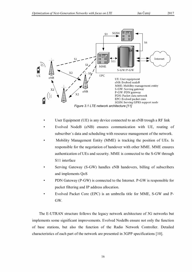
Figure 3.1 LTE network architecture [11]
• User Equipment (UE) is any device connected to an eNB trough a RF link
• Evolved NodeB (eNB) ensures communication with UE, routing of
subscriber´s data and scheduling with resource management of the network.
• Mobility Management Entity (MME) is tracking the position of UEs. Is
responsible for the negotiation of handover with other MME. MME ensures
authentication of UEs and security. MME is connected to the S-GW through
S11 interface
• Serving Gateway (S-GW) handles eNB handovers, billing of subscribers
and implements QoS
• PDN Gateway (P-GW) is connected to the Internet. P-GW is responsible for
packet filtering and IP address allocation.
• Evolved Packet Core (EPC) is an umbrella title for MME, S-GW and P-
GW.
The E-UTRAN structure follows the legacy network architecture of 3G networks but
implements some significant improvements. Evolved NodeBs ensure not only the function
of base stations, but also the function of the Radio Network Controller. Detailed
characteristics of each part of the network are presented in 3GPP specifications [10].

Optimization of Next-Generation Networks with focus on LTE Jan Černý 2017
17
4 Interference Optimization in LTE Networks
Interference mitigation has always been an important topic in cellular systems, but
LTE brings some new challenges. In order to maximize the data rate, generally the whole
frequency spectrum available for the network is assigned to each cell of the network. This
results in higher interferences around cell borders. Also, cell density increases especially in
highly populated areas. Higher cell density improves the capacity of the network and
reduces power requirements, but on the other side, higher cell density results in wider area
of high interferences around the cells borders. In addition to that, LTE networks require
higher SNIR than any previous standard. For the optimal functionality, LTE network
requires SNIR higher than 20 dB [13].
Also, LTE networks often operate on a side of other systems providing 3G, 2G or
terrestrial TV broadcasting, etc., causing inter-system interferences. This thesis will mainly
talk about inter-cell interferences. However, some of the mentioned techniques can also be
applied on inter-system interferences.
4.1 Orthogonal Frequency Division Multiple Access (OFDMA)
Data transmission over the air interface is based on the Orthogonal Frequency
Division Multiplexing (OFDM). OFDM divides frequency spectrum into multiple closely
spaced orthogonal sub-carriers.
Figure 4.1 OFDM in frequency spectrum

Optimization of Next-Generation Networks with focus on LTE Jan Černý 2017
18
Every single subcarrier can have much lower symbol rate than one carrier would have
while occupying the whole band. This efficiently eliminates the effects of multi-path.
Reflected signals do not interfere with the next symbol, because all the reflected signals
arrive during one symbol duration. To avoid any inter-symbol interference, the cyclic
prefix is implemented before every symbol. The symbols on each carrier have rectangular
character which results in SINC functions in frequency domain. To ensure no inter-carrier
interference, those carriers must be spaced in a way that the center of each carrier matches
with the zeros of all other subcarriers. This means that the subcarriers can be closely
spaced taking good advantage of the frequency spectrum. In LTE the spacing is 15 kHz.
Each subcarrier is modulated by QPSK, 16-QAM or 64-QAM and must be sampled on
the exact central frequency. The spacing frequency and the frequency of sampling must be
accurate. Therefore, OFDM is susceptible to frequency errors caused for example, by local
oscillator offset or Doppler shift.
Figure 4.2 This picture shows extension of OFDM, OFDMA. OFDMA assigns carriers to users dynamically, following their current need of bandwidth.
For the purpose of a network with many subscribers, who are accessing different
content or service at the same time, the subcarriers are dynamically assigned to the
subscribers according to their requirements and the overall traffic within the cell. The
minimal portion of subcarriers assigned to one user is called Physical Resource Block
(PRB) and consists of 12 subcarriers for 0.5 ms in duration. This period of time
corresponds to 6 or 7 OFDM symbols regarding length of implemented cyclic prefix. This
extension of OFDM called Orthogonal Frequency Division Multiple Access (OFDMA) is

Optimization of Next-Generation Networks with focus on LTE Jan Černý 2017
19
used in LTE for downlink. For uplink, a Single Carrier Frequency Division Multiple
Access (SC-FDMA) was chosen due to its better power efficiency which makes it more
suitable for use in mobile devices. [14]
4.2 Frequency Reuse
Original 2G cell networks were using frequency reuse patterns where cells had a pre-
assigned portion of available frequency spectrum. This frequency band would only be used
in spatially distant cells following a reuse pattern [15]. This approach, sometimes referred
as Hard Frequency Reuse, was chosen for its simplicity and efficiency considering the
request for stable voice service. However, it is not the most suitable technique regarding
spectral efficiency, as shown in [16]. To satisfy the increasing demand of mobile data,
Next Generation Networks required a different approach. To achieve higher maximum data
rate, the Shannon–Hartley theorem (4.1) suggests widening the frequency band.
� = � ���� �1 +�
�� [���/�] (4.1)
That is achieved by assigning the whole frequency spectrum to each cell using Full
Frequency Reuse (Figure 4.3 b and Figure 4.4 b). This inevitably results in higher inter-cell
interferences. The achievement of high data rates inside the cell is ruined by high inter-cell
interferences and low quality of reception in the cell-border areas.
Figure 4.3 Frequency reuse in special diagram: a) Hard Frequency Reuse b) Full Frequency Reuse c) Soft Frequency Reuse [17]
This is the reason why Soft Frequency Reuse (SFR) was developed. It means that the
whole frequency band is used to cover the center of the cell ensuring maximum data rate.

Optimization of Next-Generation Networks with focus on LTE Jan Černý 2017
20
The problematic areas around cell borders are served by only a part of the frequency band,
which is different in each of 3 neighborhood cells. Soft frequency reuse schemes (Figure
4.3 c and Figure 4.4 c) are often used for its efficiency especially in urban areas with high
cell density with over lapses and high number of subscribers in problematic areas.
Figure 4.4 Frequency reuse schemes in frequency spectral diagram: a) Hard Frequency Reuse b) Full Frequency Reuse c) Soft Frequency Reuse [18]
Adaptive Frequency Reuse (AFR) is an extension of Soft Frequency Reuse, where the
network can dynamically adjust to different situation as if, for example, a cell is in mode
with frequency reuse N=1 (Figure 4.3 b and Figure 4.4 b). When eNB receives information
about UEs located near the cell borders with low SNR on the downlink, it changes the
frequency reuse scheme to a similar to the presented soft frequency reuse and gives
information about it to neighborhood cells to do the same. This approach requires inter-cell
communication and it is closely interconnected with scheduling process. Deployment of
AFR can increase SNIR levels in the network about up to 10 dB. [18]
4.3 Power Control
Power control techniques have been developed since the early generations of cell
networks to save energy and prolong the battery life of the mobile devices, but mainly to
prevent interferences. In LTE, there are no intra-cell interferences due to orthogonal
character of used OFDM-based schemes. Nevertheless, inter-cell interferences are still
present and in LTE they are more critical than before, as it was previously explained.

Optimization of Next-Generation Networks with focus on LTE Jan Černý 2017
21
4.3.1 Opened and Closed Loop Power Control
There are two ways how to determine the transmission power of the UE. The first is
called Open Loop Power Control. In this scheme, the transmission power is determined
based on an algorithm implemented in UE. This algorithm considers various
characteristics, mainly the information about the maximum transmission power and path
loss of this received reference signal. Open Loop Power Control is used to determine the
initial transmission power when the connection between the UE and an eNodeB is
initialized. If the UE started to transmit maximum power, it could lead to massive
interferences causing call drops and other malfunctions. The second way is called Closed
Loop Power Control and it involves a return channel via TPC command providing
personalized feedback for each active EU. Closed Loop Power Control is used when the
connection between the UE and an eNB is established. The transmission power of the UE
is determined by the eNB and the decision is based on the information about the SNIR of
the signal. The transmission power level is updated each 20 ms via TPC command.
4.3.2 Power Control
The transmission power PPUSCH (Physical Up-line Shared Channel) is given by the
equation (4.2), where M is the number of used Physical Resource Blocks (PRBs), P0 is the
desired received power density given by network, α is the path loss compensation factor
and PL is the path loss. If the path loss compensation factor is α = 1, we talk about full
compensation of path loss. The received power from all the UEs in the cell will be the
same, unless it is limited by the maximum transmission power.
������ = 10 �����(�) + �� + � × �� [���] (4.2)
Spectral power density of this received power is given by equation (4.3), where Pn is
the noise power per PRB and SNR0 is the target signal-to-noise ratio.
����� = �� = �� + ���� [���/���] (4.3)
However, full compensation is mainly used in non-orthogonal systems, like for
example, in CDMA where equal received power helps to remove the near-far problem.

Optimization of Next-Generation Networks with focus on LTE Jan Černý 2017
22
On the other hand, in systems that use orthogonal transmission scheme it is beneficial
to use fractional compensation of path loss (0 < α < 1). In this case, the spectral power
density of this received power is given by equation (4.4).
����� = �� + �� (1 �) [���/���] (4.4)
It is apparent that the received power is decreasing with growing path loss. This
diminution depends on the path loss compensation factor as it is shown in the Figure 4.5.
The knee point is where the UE reaches the maximum transmission power allowed.
Position of this point also depends on α. [11]
Figure 4.5 Received power as a function of path loss for different values of α [11]
It has been proved, that fractional power control brings better spectral efficiency and is
especially effective in small cells up to 1 km. Fractional power control scheme generally
increases aggregate data rate of the cell up to 40% [15] and particularly improves the
situation for users on the cell edges. These users reach the maximum transmission power

Optimization of Next-Generation Networks with focus on LTE Jan Černý 2017
23
but do not experience such high interferences like they would, if users in adjacent cells,
finding themselves before the knee point, were using the full compensation scheme. [11]
4.4 Download Channel Scheduling
Modern systems like LTE do not use power control in the downlink. Instead, they
transmit with constant, often maximum power. That results in higher received power and
therefore higher data rates. This shortens the connection time necessary to transfer given
amount of data. Generated interferences are reduced via scheduling and link adaptation for
the downlink channel. Each cell receives information about interferences from
neighborhood cells via transmission-power indicator. This indicator provides information
about frequency band, where the interferences are occurring. This lets the eNB lower the
transmission power for this frequency band or switch to another one and leave this channel
free, so it does not cause interferences to any of the adjacent cells.
Scheduling provides efficient distribution of available resources among the active
UEs. Several algorithms for scheduling the UEs by the eNBs were proposed. Generally,
the more complex algorithms deliver better results. We can divide these algorithms into
channel-unaware and channel-aware. In LTE, channel-aware algorithms are used because
for wireless networks the knowledge of transmission channel is fundamental to achieve
high performance transmission. The quality of transmission is reported using CQI
(Channel Quality Indicator). [19]
4.4.1 QoS-unaware Strategies
For achieving maximum data throughput it would be logical to schedule those UE,
which are reporting favorable transmission conditions. This algorithm can be categorized
as QoS-unaware. It ensures maximum aggregate data throughput for the cell, but no
fairness to the cell-edge users and other subscribers with low-quality reception. There are
several improvements to this algorithm described in [19] that improve fairness for the UEs
with inferior signal quality.
4.4.2 QoS-aware Strategies
LTE implements QoS which facilitates the implementation of QoS based fairness
strategies for scheduling the network resources to the users. Each service has defined the

Optimization of Next-Generation Networks with focus on LTE Jan Černý 2017
24
minimum required performance. The users approaching or bellow this threshold are
scheduled with priority. Special attention must be given to VoIP service, because the
maximum acceptable delay for voice is 250 ms. Delay introduced by the network core is
about 150 ms, hence, the maximum tolerable delay over the air interface is 100 ms.
Therefore, there is a period of time, when VoIP packets have high priority. This period
however, must be reduced to the minimum length possible in order to maintain quality of
other data related services. [19]
4.5 Multiple-Input Multiple-Output (MIMO)
Theoretically, the easiest way of increasing data speed is to widen the frequency band.
Unfortunately, mobile networks providers are always limited by the bandwidth. Therefore,
a different approach to increase the speed was needed. Multiple-Input Multiple-Output
(MIMO) is one of the solutions. This name stands for the technology where multiple
antennas are transmitting multiple different data streams using the same frequency. The
antennas are detached therefore each signal has a different path. This is necessary for the
receiver to distinguish between the data streams. The rest is a matter of signal processing
on the side of the receiver. In LTE, it can be from 2 to 8 streams. In 3GPP release 13,
64 antenna-ports MIMO is studied.
This technology is already implemented in 3G but in LTE the cross-polarization was
added. This means that each of two signal waves is polarized in a plane rotated 45 degrees
from the horizontal and 90 degree to each other. Cross-polarization helps the receiver
distinguish more distorted and attenuated signals. However, MIMO still requires a lot of
data processing on the side of receiver. [14] [20]
Figure 4.6 MIMO – scenario where multiple antennas are transmitting different data streams using the same carrier but different path of propagation

Optimization of Next-Generation Networks with focus on LTE Jan Černý 2017
25
Usage of MIMO is negotiated between an UE and the eNB. There are different modes
of usage of this technology. 3GPP defines eight modes. Mode MIMO-SU is when all the
streams are received with one UE. This mode helps to increase data rate for this user. On
the other hand, MIMO-MU is when these data streams are received by different UE. This
helps to increase the capacity and efficiency of the network. Transit Diversity mode is a
slightly different approach. The same data streams are transferred over different MIMO
channels. This makes the transmission very resistant and improves the SINR. Complete
description of the MIMO transmission modes are defined in 3GPP standard or for example
in [21]. The decision of usage of MIMO is closely interconnected with scheduling
algorithms.
4.6 Beamforming
Beamforming is another way of improving spectral efficiency. With Beamforming, the
UE can be directly targeted by an antenna with a directive characteristic with an adjustable
angle. This is possible due to the deployment of antenna arrays where the antenna
characteristic can be influenced by phase shift of signals arriving to each components of
the antenna array (Figure 4.7).
Figure 4.7 Beamforming with antenna array: the UE can be directly targeted by changing the antenna characteristic [11]
The position of the UE is known to the network and therefore can be easily targeted.
This technology increases the complexity of the network, but significantly improves the
spectral efficiency, because another UE can be served by the same frequency band in the
same cell without causing interferences. The same technology can be used also for the
Optimization of Next-Generation Networks with focus on LTE Jan Černý 2017
26
uplink on the side of the eNodeB due to reciprocity of antennas. Directing the beam to the
UE increases the gain and decreases the influence of interfering signals arriving from
different directions. The deployment of Beamforming is intensively studied in 3GPP
release 13. [11] [21]
4.7 Interference Regeneration and Cancelation
Despite deployment of any previously mentioned techniques, interferences will be still
present. One possible way to repair a signal impaired by interferences is to regenerate
interfering signal and subtract it from the received signal. The interfering signal is obtained
from known reference symbol received with the data stream. This technique obviously
requires buffer and complex signal processing. Thus, the Interference Cancelation (IC) is
mainly implemented only in the base stations and used for uplink. It helps to fight not only
interferences from adjacent cells, but also any other type of interferences.
4.8 Signal Quality Values and Adaptive Modulation and Coding
Another factor defining the data speed is the number of bits per symbol, which is
given by the used modulation. Modulations used in LTE are QPSK, 16-QAM or 64-QAM.
LTE advanced is adding 128-QAM and 256-QAM, but these high orders of modulation are
currently supported only by premium mobile phones. Adaptive Modulation and Coding
(AMC) is responsible for choosing the highest modulation possible with respect to the
current channel characteristics. 64-QAM modulation provides 6 bits per symbol, but the
transmission becomes more sensitive to noise. Therefore, in case of worse signal
conditions, a modulation with lower number of bits per symbol is chosen to keep an
acceptable bit error rate. This system ensures maximum data speed in an area of good
coverage and stable error-free connection in an area with weaker signal and/or lower
Signal-to-Noise-plus-Interference-Ratio (SNIR). This typically happens on the cell edges.
[11]
The level of received power is reported by the UE using RSRP (Reference Signal
Received Power) number. RSRP depends on the power of received reference signal from
the eNodeB and it is defined in a range from -140 dBm to -44 dBm with a step of 1 dBm.

Optimization of Next-Generation Networks with focus on LTE Jan Černý 2017
27
The quality of the signal is expressed by RSRQ (Reference Signal Received Quality)
which is a result of formula (4.5), where N is the number of used resource blocks (PRBs)
and RSSI (Received Signal Strength Indicator) is the overall received power by the UE
including the interfering signals. RSRQ is defined in the range from -3 dB to -19.5 dB.
[22]
���� = �����
���� (4.5)
Tab. 4-1 Relation between RSRP, RSRQ and SINR and meaning of values of these indicators [28]
RSRP [dBm] RSRQ [dB] SINR [dB]
RF
Con
dit
ion
s
Excelent ≥ -80 ≥ -10 ≥ 20
Good -80 to -90 -10 to -15 13 to 20
Mid Cell -90 to -100 -15 to -20 0 to 100
Cell Edge ≤ -100 ≤ -20 ≤ 0
eNodeB chooses the order of modulation according to the CQI (Channel Quality
Indicator) number. CQI value varies in the range from 0 to 15. CQI is estimated by the UE
based on the SINR conditions and capability of the device to achieve block error rate lower
than 10%. CQI=0 means out of range, up to CQI=6 QPSK is used, for CQI values from 7
to 9 16-QAM is used and from CQI=10 64-QAM can be used, if the UE supports it. [23]
5 LTE Network Planning
Mobile network is a very complex and therefore expensive technological system. Any
mistake made during the process of planning the network results in increase of costs,
degradation of the efficiency in the whole building process and network performance. The
goal of network planning is to establish a radio network with sufficient coverage and
capacity to ensure expected quality of service. All the resources must be used with the
maximum efficiency. Therefore, the particular area must be carefully studied in terms of
population density, geographical and residential character. Already existing networks must
be taken in account. Well planned network should be also prepared for possible future
development.
Optimization of Next-Generation Networks with focus on LTE Jan Černý 2017
28
5.1 Cell Site Planning
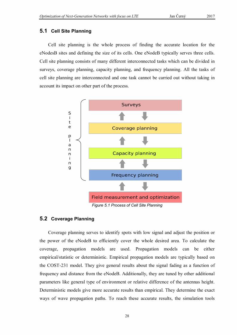
Cell site planning is the whole process of finding the accurate location for the
eNodesB sites and defining the size of its cells. One eNodeB typically serves three cells.
Cell site planning consists of many different interconnected tasks which can be divided in
surveys, coverage planning, capacity planning, and frequency planning. All the tasks of
cell site planning are interconnected and one task cannot be carried out without taking in
account its impact on other part of the process.
Figure 5.1 Process of Cell Site Planning
5.2 Coverage Planning
Coverage planning serves to identify spots with low signal and adjust the position or
the power of the eNodeB to efficiently cover the whole desired area. To calculate the
coverage, propagation models are used. Propagation models can be either
empirical/statistic or deterministic. Empirical propagation models are typically based on
the COST-231 model. They give general results about the signal fading as a function of
frequency and distance from the eNodeB. Additionally, they are tuned by other additional
parameters like general type of environment or relative difference of the antennas height.
Deterministic models give more accurate results than empirical. They determine the exact
ways of wave propagation paths. To reach these accurate results, the simulation tools

Optimization of Next-Generation Networks with focus on LTE Jan Černý 2017
29
require more specific data about the area and they are more demanding on computing
resources. Three-dimensional ray tracing is an example of deterministic model used in
LTE planning. To reach higher accuracy when planning, an additional field measurement
must be carried out to verify and adjust the results of the simulation. Choice of frequency
has also impact on coverage. Higher frequencies have higher path loss and therefore, the
maximum size of a cell is smaller. [11]
5.3 Capacity Planning
Capacity planning of LTE networks is usually based on measured data obtained from
an existing network. The capacity of a cell is limited and one cell can handle only a limited
number of subscribers. Therefore, in areas with higher expected traffic (for example a city
center) the cell size must be smaller compared to suburban or rural areas.
The arrival of smartphones brought completely new challenges for capacity planning.
Smartphones are constantly going from idle state to connected, when applications
synchronize with a server. They are also more demanding on data speed and therefore
require more bandwidth. [11]
To ensure maximum data speed but also to satisfy maximum users, the bandwidth is
assigned dynamically (see 4.1 OFDMA). With more active users in a cell the data speed
for one user degrades. To deliver important real time services, as for example voice or
video-call in conditions of higher cell traffic, a well-defined Quality of Services protocol
must be implemented. With increasing traffic in the network the interference grows, which
has also significant impact on capacity. Interferences can be limited with correct frequency
planning. [14] [11]
5.4 Frequency Planning
3GPP defines various frequency bands in range from 700 MHz to 3800 MHz. It also
defines different bands for Frequency Division Duplex (FDD) and for Time Division
Duplex (FDD). The used bandwidth can be 1.4 MHz, 3 MHz, 5 MHz, 10 MHz, 15 MHz or
20 MHz. This gives the operators a possibility to implement frequency band available in
their area.

Optimization of Next-Generation Networks with focus on LTE Jan Černý 2017
30
Instead of using different frequency carriers in adjacent cells, like for example in
GSM, in LTE Full Frequency Reuse scheme can be used. Then the whole frequency band
is assigned to each cell. That improves the capacity of each cell but results in higher
interference on the borders of the cells. LTE uses scrambling and pseudo-noise codes to
distinguish between signals on the same frequency [11]. Still the interferences are present
and result in noise which according to the Shannon-Hartley theorem degrades maximum
possible data throughput. Therefore, in urban areas with high site density it is
recommended to use Soft Frequency Reuse scheme (see 4.2 Frequency Reuse).
5.5 Professional Software for Network Planning
To help the engineers with all the complex tasks connected with the network design
there are various Radio Network Planning (RNP) software tools. Based on information
about the network configuration and characteristics of the environment, the RNP tool
provides graphical outputs visualizing coverage, capacity and interference in the network
area. RNP software tools must contain characteristics of used network standard and
equipment to give applicable results. Therefore, the proper planning software tools must be
used for planning of LTE networks. According to [25] and [26] the most popular RNP
software is Atoll. Atoll is a multi-technology wireless network design and optimization
software tool suitable for many standards including GSM, UMTS and LTE. It supports
multi-technology simulation suitable for planning LTE networks along with other
standards. It also includes various adjustable propagation models both empirical and
deterministic. Atoll also supports various sources of geographical data including popular
web map services. Other wide spread software tools are for example ASSET or Pegaplan
[27].
There is an example of the coverage calculation in the Figure 5.3. The result shows the
achievable data rate which a user can achieve at a certain location in a radio network with a
certain probability. This means, that this achievable data rate is calculated for every pixel
of the map. [27]

Optimization of Next-Generation Networks with focus on LTE Jan Černý 2017
31
Figure 5.2 Radio Network Planning tool calculates and visualizes its outputs based on introduced data about the network configuration and the particular environment [24]
Figure 5.3 Example of coverage map output [27]
Optimization of Next-Generation Networks with focus on LTE Jan Černý 2017
32
6 Simulation of LTE Network Optimization
In order to demonstrate and visualize the impact of interferences on the network
functionality, a simulation in MATLAB was created. The objective is to take into account
propagation loss, MIMO and AMC and show the direct relation between the level of
interferences and the network data throughput. Power control technology and scheduling
are not implemented. This means that the antennas are assumed to be transmiting
maximum power the whole time in the whole assigned frequency spectrum.
6.1 Functionality of Simulation Program
In the Figure 6.2 we can see the simulation program with a prepared scenario. The
program gets to this stage after loading the jpg file with a map by clicking on “Open file
with map”. The size of the scenario can be modified by changing the dimensions. After
clicking on “Show Scenario”, the map appears. Positions with information about eNBs are
loaded from file posT.txt and shown. The eNBs can be modified, added or deleted by the
group of buttons called “Edit Scenario”.
After choosing to add an eNB, user is prompted to right-click to the point where new
eNB is supposed to be placed. Then, a query to determine characteristics of antennas
appears for each of 3 sectors (Figure 6.1). Different transmitted power, bandwidth and
frequency can be assigned to each sector and respective antenna. The same query appears
when a sector is edited however, the sectors are edited separately.
When the scenario is prepared, the coverage is calculated either by using COST-231
model or Okumura-Hata model with corrections for city, suburban areas or countryside.
Used formulas can be found in [29]. The coverage can be displayed for each point, or only
for those with sufficient signal level. Signal stronger than introduced “Threshold” is
considered sufficient.
However, quality of the signal is determined by SINR (see 4.8). Therefore,
interferences are evaluated in the next step. SINR is calculated as the ratio between the
strongest signal and second strongest signal of the same frequency. The final value of
SINR for each point is taken for the frequency with highest SINR.

Optimization of Next-Generation Networks with focus on LTE Jan Černý 2017
33
Figure 6.1 Process of creating a scenario
Figure 6.2 Simulation program with a created scenario
Based on the calculated SINR, the throughput of the network is determined using an
algorithm approaching the AMC technology. For areas with SINR over the 64QAM
threshold the 6-bit modulation is used. In areas with SINR between the 64QAM Threshold
and the 16QAM Threshold the 4-bit modulation is used, for areas with SINR under the
16QAM Threshold 2-bit QPSK modulation is used. Also in areas with SINR under the
Diversity Mode Threshold, the MIMO technology does not improve the throughput.
Optimization of Next-Generation Networks with focus on LTE Jan Černý 2017
34
6.2 Simulation Results
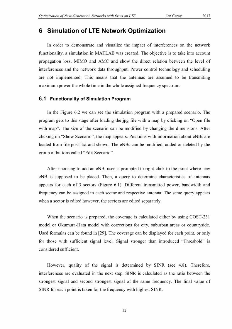
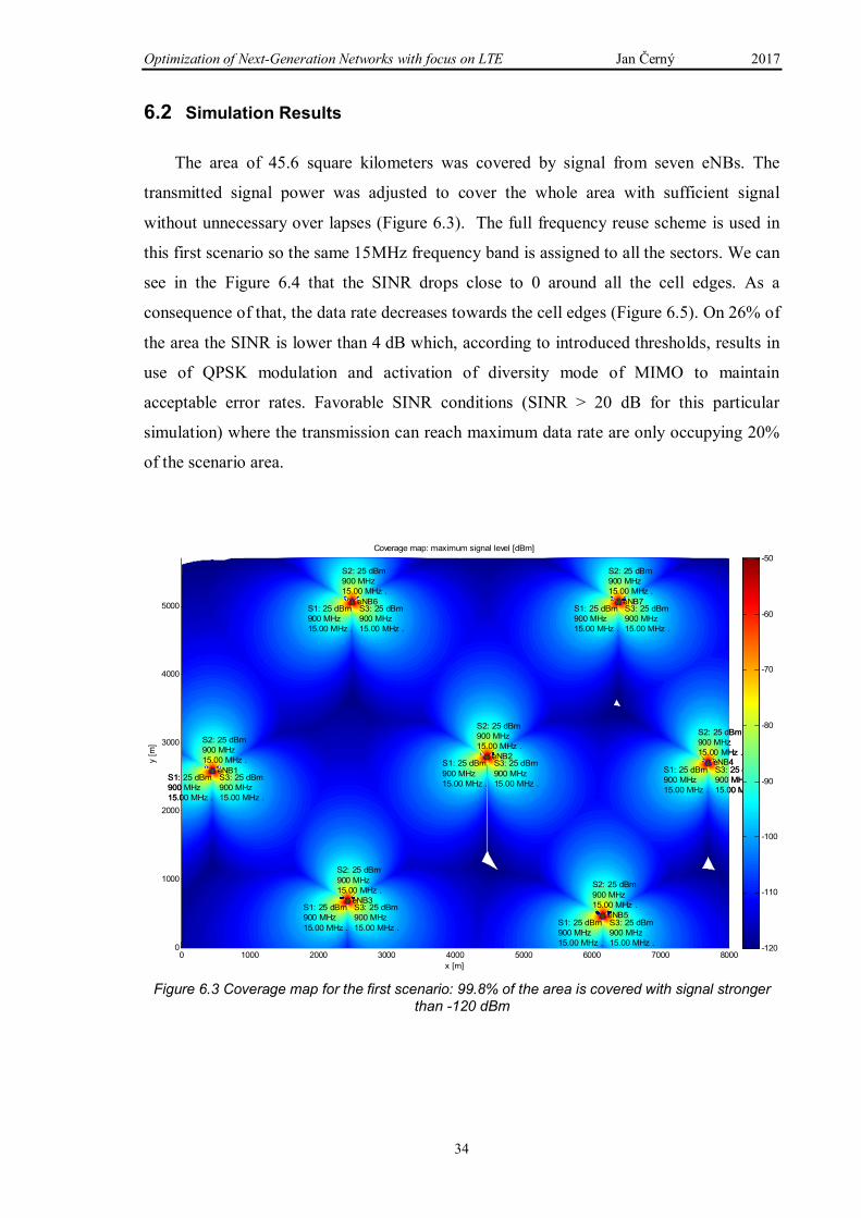
The area of 45.6 square kilometers was covered by signal from seven eNBs. The
transmitted signal power was adjusted to cover the whole area with sufficient signal
without unnecessary over lapses (Figure 6.3). The full frequency reuse scheme is used in
this first scenario so the same 15MHz frequency band is assigned to all the sectors. We can
see in the Figure 6.4 that the SINR drops close to 0 around all the cell edges. As a
consequence of that, the data rate decreases towards the cell edges (Figure 6.5). On 26% of
the area the SINR is lower than 4 dB which, according to introduced thresholds, results in
use of QPSK modulation and activation of diversity mode of MIMO to maintain
acceptable error rates. Favorable SINR conditions (SINR > 20 dB for this particular
simulation) where the transmission can reach maximum data rate are only occupying 20%
of the scenario area.
Figure 6.3 Coverage map for the first scenario: 99.8% of the area is covered with signal stronger than -120 dBm
0 1000 2000 3000 4000 5000 6000 7000 80000
1000
2000
3000
4000
5000
x [m]
y [
m]
Coverage map: maximum signal level [dBm]
eNB1S1: 25 dBm900 MHz 15.00 MHz .
S2: 25 dBm900 MHz 15.00 MHz .
S3: 25 dBm900 MHz 15.00 MHz .
eNB2S1: 25 dBm
900 MHz 15.00 MHz .
S2: 25 dBm900 MHz 15.00 MHz .
S3: 25 dBm
900 MHz 15.00 MHz .
eNB3S1: 25 dBm900 MHz
15.00 MHz .
S2: 25 dBm
900 MHz 15.00 MHz .
S3: 25 dBm900 MHz
15.00 MHz .
eNB4S1: 25 dBm900 MHz 15.00 MHz .
S2: 25 dBm900 MHz 15.00 MHz .
S3: 25 dBm900 MHz 15.00 MHz .
eNB5S1: 25 dBm900 MHz 15.00 MHz .
S2: 25 dBm
900 MHz 15.00 MHz .
S3: 25 dBm900 MHz 15.00 MHz .
eNB6S1: 25 dBm900 MHz 15.00 MHz .
S2: 25 dBm900 MHz 15.00 MHz .
S3: 25 dBm900 MHz 15.00 MHz .
eNB7S1: 25 dBm900 MHz 15.00 MHz .
S2: 25 dBm900 MHz 15.00 MHz .
S3: 25 dBm900 MHz 15.00 MHz .
-120
-110
-100
-90
-80
-70
-60
-50
Optimization of Next-Generation Networks with focus on LTE Jan Černý 2017
35
Figure 6.4 SINR map for the first scenario: SINR drops significantly around the cell edges
Figure 6.5 Data rate map for the first scenario: 20% of the area allows up to 151.2 Mbps, 26% of surface around cell borders only 25.2 Mbps due to low SINR
0 1000 2000 3000 4000 5000 6000 7000 80000
1000
2000
3000
4000
5000
x [m]
y [
m]
SINR [dB]
eNB1S1: 25 dBm900 MHz 15.00 MHz .
S2: 25 dBm900 MHz 15.00 MHz .
S3: 25 dBm900 MHz 15.00 MHz .
eNB2S1: 25 dBm
900 MHz 15.00 MHz .
S2: 25 dBm900 MHz 15.00 MHz .
S3: 25 dBm
900 MHz 15.00 MHz .
eNB3S1: 25 dBm900 MHz 15.00 MHz .
S2: 25 dBm900 MHz 15.00 MHz .
S3: 25 dBm900 MHz 15.00 MHz .
eNB4S1: 25 dBm900 MHz 15.00 MHz .
S2: 25 dBm900 MHz 15.00 MHz .
S3: 25 dBm900 MHz 15.00 MHz .
eNB5S1: 25 dBm900 MHz 15.00 MHz .
S2: 25 dBm900 MHz 15.00 MHz .
S3: 25 dBm900 MHz 15.00 MHz .
eNB6S1: 25 dBm900 MHz
15.00 MHz .
S2: 25 dBm
900 MHz 15.00 MHz .
S3: 25 dBm900 MHz
15.00 MHz .
eNB7S1: 25 dBm900 MHz
15.00 MHz .
S2: 25 dBm
900 MHz 15.00 MHz .
S3: 25 dBm900 MHz
15.00 MHz .
0
10
20
30
40
50
60
70
x [m]
y [
m]
Throughput of LTE network [Mbps]
eNB1S1: 25 dBm
900 MHz 15.00 MHz .
S2: 25 dBm900 MHz
15.00 MHz .
S3: 25 dBm
900 MHz 15.00 MHz .
eNB2S1: 25 dBm900 MHz
15.00 MHz .
S2: 25 dBm
900 MHz 15.00 MHz .
S3: 25 dBm900 MHz
15.00 MHz .
eNB3S1: 25 dBm900 MHz
15.00 MHz .
S2: 25 dBm900 MHz 15.00 MHz .
S3: 25 dBm900 MHz
15.00 MHz .
eNB4S1: 25 dBm
900 MHz 15.00 MHz .
S2: 25 dBm900 MHz
15.00 MHz .
S3: 25 dBm
900 MHz 15.00 MHz .
eNB5S1: 25 dBm
900 MHz 15.00 MHz .
S2: 25 dBm900 MHz
15.00 MHz .
S3: 25 dBm
900 MHz 15.00 MHz .
eNB6S1: 25 dBm
900 MHz 15.00 MHz .
S2: 25 dBm900 MHz
15.00 MHz .
S3: 25 dBm
900 MHz 15.00 MHz .
eNB7S1: 25 dBm
900 MHz 15.00 MHz .
S2: 25 dBm900 MHz
15.00 MHz .
S3: 25 dBm
900 MHz 15.00 MHz .
0 1000 2000 3000 4000 5000 6000 7000 80000
1000
2000
3000
4000
5000
40
60
80
100
120
140
Optimization of Next-Generation Networks with focus on LTE Jan Černý 2017
36
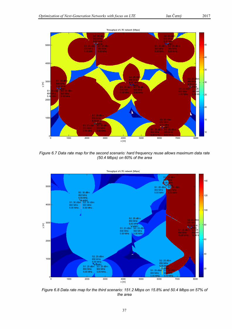
The same area was covered again by eNBs using hard frequency reuse. Cells are
covered by antennas using 5 MHz bandwidth. This frequency band is different for each
sector of an eNB, following the frequency reuse scheme. In this case, SINR improved
significantly in the whole area. Consequently, the area where the maximum speed
connection can be delivered is 60% for this scenario (Figure 6.7). However, the maximum
data rate is lower in the whole area due to the bandwidth being reduced to 5 MHz. On the
other hand, the area with critical SINR, where MIMO would switch to diversity mode, is
minimal. This means that the connection will be more stable and less vulnerable to
interferences of other sources, (which are not included in the simulation), or to fading.
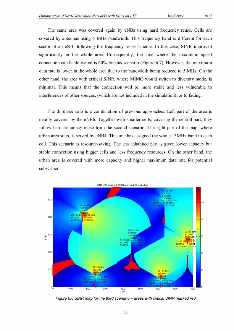
The third scenario is a combination of previous approaches. Left part of the area is
mainly covered by the eNB6. Together with smaller cells, covering the central part, they
follow hard frequency reuse from the second scenario. The right part of the map, where
urban area stars, is served by eNB4. This one has assigned the whole 15MHz band to each
cell. This scenario is resource-saving. The less inhabited part is given lower capacity but
stable connection using bigger cells and less frequency resources. On the other hand, the
urban area is covered with more capacity and higher maximum data rate for potential
subscriber.
Figure 6.6 SINR map for the third scenario – areas with critical SINR marked red
0 1000 2000 3000 4000 5000 6000 7000 80000
1000
2000
3000
4000
5000
x [m]
y [
m]
SINR [dB], areas with SINR lower than4 dB marked red
eNB1S1: 25 dBm800 MHz 5.00 MHz .
S2: 25 dBm850 MHz 5.00 MHz .
S3: 25 dBm900 MHz 5.00 MHz .
eNB2S1: 25 dBm800 MHz 5.00 MHz .
S2: 25 dBm
850 MHz 5.00 MHz .
S3: 25 dBm900 MHz 5.00 MHz .
eNB3S1: 25 dBm800 MHz 15.00 MHz .
S2: 25 dBm
800 MHz 15.00 MHz .
S3: 25 dBm800 MHz 15.00 MHz .
eNB4S1: 25 dBm800 MHz 5.00 MHz .
S2: 25 dBm850 MHz 5.00 MHz .
S3: 25 dBm900 MHz 5.00 MHz .
eNB5S1: 25 dBm800 MHz 5.00 MHz .
S2: 25 dBm
850 MHz 5.00 MHz .
S3: 25 dBm900 MHz 5.00 MHz .
eNB6S1: 30 dBm800 MHz 5.00 MHz .
S2: 30 dBm850 MHz 5.00 MHz .
S3: 30 dBm900 MHz 5.00 MHz .
0
20
40
60
80
100
Optimization of Next-Generation Networks with focus on LTE Jan Černý 2017
37
Figure 6.7 Data rate map for the second scenario: hard frequency reuse allows maximum data rate (50.4 Mbps) on 60% of the area
Figure 6.8 Data rate map for the third scenario: 151.2 Mbps on 15.8% and 50.4 Mbps on 57% of the area
x [m]
y [m
]
Throughput of LTE network [Mbps]
eNB1S1: 25 dBm800 MHz 5.00 MHz .
S2: 25 dBm850 MHz 5.00 MHz .
S3: 25 dBm900 MHz 5.00 MHz .
eNB2S1: 25 dBm800 MHz 5.00 MHz .
S2: 25 dBm850 MHz 5.00 MHz .
S3: 25 dBm900 MHz 5.00 MHz .
eNB3S1: 25 dBm800 MHz 5.00 MHz .
S2: 25 dBm850 MHz 5.00 MHz .
S3: 25 dBm900 MHz 5.00 MHz .
eNB4S1: 25 dBm800 MHz 5.00 MHz .
S2: 25 dBm850 MHz 5.00 MHz .
S3: 25 dBm900 MHz 5.00 MHz .
eNB5S1: 25 dBm800 MHz 5.00 MHz .
S2: 25 dBm850 MHz 5.00 MHz .
S3: 25 dBm900 MHz 5.00 MHz .
eNB6S1: 25 dBm800 MHz 5.00 MHz .
S2: 25 dBm850 MHz 5.00 MHz .
S3: 25 dBm900 MHz 5.00 MHz .
eNB7S1: 25 dBm800 MHz 5.00 MHz .
S2: 25 dBm850 MHz 5.00 MHz .
S3: 25 dBm900 MHz 5.00 MHz .
0 1000 2000 3000 4000 5000 6000 7000 80000
1000
2000
3000
4000
5000
10
15
20
25
30
35
40
45
x [m]
y [
m]
Throughput of LTE network [Mbps]
eNB1S1: 25 dBm800 MHz 5.00 MHz .
S2: 25 dBm850 MHz 5.00 MHz .
S3: 25 dBm900 MHz 5.00 MHz .
eNB2S1: 25 dBm800 MHz 5.00 MHz .
S2: 25 dBm850 MHz 5.00 MHz .
S3: 25 dBm900 MHz 5.00 MHz .
eNB3S1: 25 dBm800 MHz 15.00 MHz .
S2: 25 dBm800 MHz 15.00 MHz .
S3: 25 dBm800 MHz 15.00 MHz .
eNB4S1: 25 dBm800 MHz 5.00 MHz .
S2: 25 dBm850 MHz 5.00 MHz .
S3: 25 dBm900 MHz 5.00 MHz .
eNB5S1: 25 dBm800 MHz 5.00 MHz .
S2: 25 dBm850 MHz 5.00 MHz .
S3: 25 dBm900 MHz 5.00 MHz .
eNB6S1: 30 dBm800 MHz 5.00 MHz .
S2: 30 dBm850 MHz 5.00 MHz .
S3: 30 dBm900 MHz 5.00 MHz .
0 1000 2000 3000 4000 5000 6000 7000 80000
1000
2000
3000
4000
5000
20
40
60
80
100
120
140

Optimization of Next-Generation Networks with focus on LTE Jan Černý 2017
38
Critical areas with low SINR (Figure 6.6), although minimal, are still present in the
third scenario. This would be improved by deployment of power control and scheduling.
Data rates of the inside areas of the cells could be improved by implementation of soft
frequency reuse.
6.3 Technical Realization of the Simulation Program
The simulation was created in MATLAB based on simulation of coverage for GSM
networks [29]. The program consists of 15 user functions and one secondary user interface
(Attachment B). The functions are called from the main program “Simulation_LTE.m”.
The main program is interconnected with the user interface file “Simulation_LTE.fig”.
Code of all the functions together with their overview is contained in the attachments of
this thesis.
All the important variables (Attachment C) are stored in the structure “s” as a part of
handles of the GUI figure. Coverage maps are stored as two or three dimensional matrixes,
where each element presents value for one square meter. MATLAB build-in functions for
matrix operations are used preferably for their good performance. The disadvantage of this
approach is that a single variable can occupy a lot of memory. Data is mainly stored as
16-bit integer. However, signal coverage maps are stored as the 32-bite single data type to
avoid discontinuity in the presented coverage maps. In the created scenario with
dimensions of 8000 per 5700 meters and 21 antennas, the program generates coverage
maps of 3.83 GB. MATLAB can run into an error for lack of RAM memory while
simulating extensive scenarios. In some cases, loops running over these matrixes had to be
created. This results in time consuming operations. The most critical task is the calculation
of signal coverage, which took approximately 3 minutes on the computer (2.50 GHz, 24
GB RAM) utilized to simulate the presented scenarios, while the rest of the tasks took up
to 30 seconds. These intervals may vary with the particular PC´s performance and
scenario.
6.3.1 Calculation of coverage
Coverage is calculated based on distance from the transmitter and asigned frequency
using the COST-231 or the Okumura-Hata model [29]. The effective height of transmitting
antennas is fixed on 30 meters and receiving height on 2 meters. Choice of environment in

Optimization of Next-Generation Networks with focus on LTE Jan Černý 2017
39
the user interface has effect on the propagation via correction parameters. Both models are
fully valid from 1 km distance. The Okumura-Hata model is only designed for frequency
range 150 MHz – 1500 MHz. Therefore, for higher frequencies it is necessary to use the
COST-231 model, which is valid for frequencies between 1500 MHz and 2000 MHz.
There are more sophisticated models for LTE planning, but they require more input
variables, which are not available in this simulation. These models can be found in [11].
The level of the signal is calculated for each of the used frequency bands and stored in
variable “signalmap” as a three-dimensional matrix. Maximum for each point of the map is
found and stored in two-dimensional matrix “maxmap”. This matrix is presented
graphically as the coverage map in the first step of the simulation. After the calculation of
coverage, the percentage of covered area is printed to MATLAB command window.
6.3.2 Antenna Characteristics
LTE networks use antenna arrays. Their patterns can be adjusted with phase shift of
signals for each element. The pattern of antenna arrays used in this simulation was
modeled using parameterized Sinc function (6.1). Parameter a is adjusting the beam width
and b the directivity.
Mag = ����(� � � �)� [��] (6.1)
The pattern of four-element antenna [30] is compared with adjusted Sinc function in
the Figure 6.9. It is visible, that they are practically identical, however Sinc function
creates more side lobes to all the directions. For the simulation, side lobes are removed and
the beam width is adjusted to cover 120° sector.

Optimization of Next-Generation Networks with focus on LTE Jan Černý 2017
40
Figure 6.9 Pattern of antenna array (right) was approximated with parameterized sinc function (left)
6.3.3 Calculation of SINR
The SINR is calculated as the ratio of the strongest signal to the second strongest
signal with the same frequency. If there is no interfering signal with the same frequency,
the interfering signal is the noise. The noise level is calculated with formula (6.2) based on
introduced noise value and bandwidth of the antenna. This SINR map is calculated for
each frequency. In the end, the maximum value for each point is found and stored as a two-
dimensional matrix in the variable “CI_dB”.
� = ����� + 10��� (�) [���/��, ��, ���] (6.2)
This way, the simulation is trying to find the best signal that would be available to a
potential UE in each point of the simulated area.
6.3.4 Implementation of AMC and MIMO
Data rate is calculated based on previously calculated SINR. The number of available
resource blocks for each sector is determined based on the bandwidth value stored in
variable “posT” with other information about the antenna. Adaptive modulation is
implemented and for SNIR < “16QAM Threshold” the QPSK modulation schema is used,
for “16QAM Threshold” < SINR < “64QAM Threshold” the 16QAM is used and for areas
with SINR > “64QAM Threshold” the 64QAM modulation is used. These thresholds have
-80 -60 -40 -20 0 20 40 60 80-40
-35
-30
-25
-20
-15
-10
-5
0APROXIMATION WITH PARAMETRIZED SINC
Theta [°]
Mag
nitu
de
[dB
]
0 20 40 60 80 100 120 140 160 180-40
-35
-30
-25
-20
-15
-10
-5
0RADIATION PATTERN WITH 4 ELEMENTS
Theta [°]
Mag
nitu
de
[dB
]

Optimization of Next-Generation Networks with focus on LTE Jan Černý 2017
41
to be estimated because they are not standardized and in reality the order of modulation is
decided by the UE and depends on the particular capability of the device.
MIMO technology is taken into account while calculating the throughput. User can
choose from MIMO-MU mode, MIMO 2x2 or 4x4. MIMO-MU does not improve the data
rate for single user but network´s capacity. MIMO 2x2 increases the throughput two times
and MIMO 4x4 four times for one hypothetical user. In areas with SINR level under the
“Threshold for diversity mode” the data speed drops, which simulates the passage to
diversity mode where MIMO helps to fight low SINR and does not directly improve data
throughput.
75 12 7 2 6 2 = 151200 [��� ����] (6.3)
To give an example of data throughput calculation, we can assume 15MHz bandwidth.
That means 75 Physical Resource Blocks (PRBs). Each of PRBs consists of 12 subcarriers.
There are 7 symbols per subcarrier (assuming normal cyclic prefix). Each symbol is
transmitted in a 0.5 ms slot. If 2x2 MIMO is used, then the maximum data rate in the
location with excellent reception, where 64QAM carrying 6 bits per symbol can be used, is
calculated as (6.3).

Optimization of Next-Generation Networks with focus on LTE Jan Černý 2017
42
Conclusion
The main goal of this thesis was to explore the technologies used for interference
optimization and mitigation and simulate their effect on data throughput. On the presented
simulation, is visible how important network optimization and deployment of technologies
capable of increasing spectral efficiency and therefore avoiding interferences is. In a purely
optimized network, the whole potential of high data rates would be ruined by interferences
in mayor part of the networks area. Therefore, technologies as power control, scheduling
algorithms and frequency reuse have been investigated, improved and deployed in LTE.
AMC and MIMO technologies are being continuously developed and there are some new
technologies in LTE as, for example, adaptive beam forming. Although all these
technologies have been brought to maximum efficiency, it is necessary to combine various
types of technologies and a quality scheduling algorithm to achieve a functional and
efficient network with reuse pattern close to N=1 in order to deliver maximum throughput.
Network optimization is a part of the network planning process. LTE networks are
very complex and their planning takes into account many factors. All the tasks of site
planning (coverage planning, capacity planning, frequency planning) are interconnected
and cannot be carried out separately. Professionally used Radio Network Planning tools are
complex and expensive programs. They are able to visualize coverage, capacity and
potential data rates in the planned network based on introduced configuration and
environment characteristics. Still, it is essential to verify and adjust the results by field
measurements.
The results of the created simulation successfully visualize the impact of interferences
on data throughput of LTE network and importance of network optimization. A purely
optimized network is not using resources efectively and a lack of optimization could lead
to malfunction. The first presented scenario is using a maximum of resources but the
functionality is degraded by interferences in a large area of the network. The situation is
improved in the third scenario by a combination of frequency reuse techniques and by
adjusting the sizes of the cells. However, this result would not be fully satisfying and it is
apparent that the implementation of other technologies to the network, as scheduling and
power control, is needed.

Optimization of Next-Generation Networks with focus on LTE Jan Černý 2017
43
These technologies were not implemented in the simulation, mainly because of their
complexity. To implement them, statistical data would be required. This data is not
publicly accessible and it is a part of knowhow of companies creating the professional
software and those who are implementing these technologies in the mobile networks. It
was also not possible to visualize the advantages of soft frequency reuse due to the created
algorithm, which prioritizes stronger signal. To do so, the program would have to be
modified to calculate data rate maps for all the frequencies and find the maximum value
for each point. This improvement would make the simulation more demanding on memory
and computing time. The memory requirements would be reduced by usage of 16-bit
integer for signal coverage maps, but that would create unnatural discontinuity in the
simulation results.
The original simulation of coverage for GSM networks [29] was significantly
modified, optimized and adapted for simulations of LTE networks. The results of the
simulation give graphic visualization on how the deployment of AMC and various modes
of MIMO technology affect the data throughput. These technologies react on SINR level to
maintain an acceptable error rate. This interconnection is well visible from the simulation
outputs. Therefore, the task of this thesis can be considered as fulfilled, although the
simulation could be continuously improved to approach such a complicated system as an
LTE communication network undoubtedly is.

Optimization of Next-Generation Networks with focus on LTE Jan Černý 2017
44
Literature and Sources
[1] Ericsson. Ericsson Mobility Report [online]. June 2015 [Retrieved Feb. 24, 2016]. Available from: http://www.ericsson.com/res/docs/2015/ericsson-mobility-report-june-2015.pdf
[2] Ericsson. Ericsson Mobility Report [online]. June 2016 [Retrieved March 16, 2017]. Available from: https://www.ericsson.com/res/docs/2016/ericsson-mobility-report-2016.pdf
[3] EBERLE, Dieter. LTE vs. WiMAX 4th generation telecommunication networks [online]. [Retrieved March 20, 2017]. Available from: https://www.snet.tu-berlin.de/fileadmin/fg220/courses/WS1011/snet-project/lte-vs-wimax_eberle.pdf
[4] Reuters. Qualcomm halts UMB project [online] November 13th, 2008 [Retrieved March 20, 2017]. Available from: http://uk.reuters.com/article/qualcomm-umb-idUKN1335969420081113
[5] GSA, Evolution to LTE report [online]. [Retrieved March 20, 2017]. Available from: http://gsacom.com/paper/gsa-evolution-to-lte-report-january-25-2016-480-lte-networks-launched-in-157-countries/
[6] BERNKOPF, J. Femto cells in Next Generation mobile networks: Master´s thesis. Brno: University Of Technology, Faculty of Electrical Engineering and Communication, 2010
[7] UNZEITIG, L. Cellular Network Coverage Model: Master´s thesis Brno: University Of Technology, Faculty of Electrical Engineering and Communication, 2008
[8] PÉREZ, F. F. and ESPIÑERA P. M. Modelling the Wireless Propagation Channel: A simulation approach with Matlab. 2008 ISBN: 978-0-470-75173-2
[9] ZARRRINKOUB, H. Understanding LTE with MATLAB: From Mathematical Modeling to Simulation Prototyping. March 2014. 508 pages. ISBN: 978-1-118-44341-5
[10] 3GPP [online]. [Retrieved March 20, 2017]. Available from: http://www.3gpp.org
[11] L. Song, J. Shen, M. Stasiak, P. Zwierzykowski and M. Głąbowski. Evolved celluar network planning and optimization for UMTS and LTE. Boca Raton, CRC Press, Taylor & Francis Group, 2011
[12] Requirements for E-UTRA and E-UTRAN. 3GPP TR 25.913 version 7.3.0 Release 7, April 2013
[13] CommScope. LTE Best Practices [Ebook]. March 2015
[14] Huawei. Long Term Evolution (LTE) Radio Access Network Planning Guide [online]. 2011. [Retrieved March 1, 2016]. Available from: http://www.slideshare.net/tharinduwije/lte-radio-netwok-planning
[15] S. Engström, T. Johanson, F. Kronestedt, M. Larsson, S. Lidbrink, H. Olofsson. Multiple Reuse Patterns for Frequency Planning in GSM Networks. IEEE VTC'98, pp. 2004-2008, 1998-May
[16] KWANG, R. and LEUNG, C. A Survey of Scheduling and Interference Mitigation in LTE. 2010.

Optimization of Next-Generation Networks with focus on LTE Jan Černý 2017
45
[17] HUADONG, C. LTE Network Design and Deployment Strategy [online]. 2011. [Retrieved December 20, 2016]. Available from: http://wwwen.zte.com.cn/endata/magazine/ztetechnologies/2011/no1/articles/201101/t20110117_201779.html
[18] G. Boudreau, J. Panicker, N. Guo, R. Chang, N. Wang and S. Vrzic. Interference Coordination and Cancellation for 4G Networks. IEEE Communications Magazine, vol. 47, no. 4, April 2009
[19] F. Capozzi, G. Piro, L.A. Grieco, G. Boggia, P. Camarda. Downlink Packet Scheduling in LTE Cellular Networks: Key Design Issues and a Survey. IEEE Commun. Surveys and Tutorials., 15 (2) (2012), pp. 678-700
[20] Telco Antennas. What is MIMO? [online]. [Retrieved March 07, 2016]. Available from: https://www.telcoantennas.com.au/site/how-does-mimo-work
[21] SCHULZ, B. LTE Transmission modes and Beamforming. Rohde & Schwarz White Paper, July 2015
[22] E-UTRAN, Requirements for support of radio resource management, 3GPP TS 36.133 version 8.9.0 Release 8, April 2010
[23] SAINJU, Prabhat M. LTE Performance Analysis on 800 and 1800 MHz Bands. Tampere University of Technology, September 2012
[24] PIETRZYK, S. LTE Radio Network Planning Tutorial [online]. 2012 [Retrieved February 18, 2016]. Available from: http://www.slideshare.net/IS-Wireless/lte-radio-network-planning-tutorial-from-iswireless?qid=4fb71c09-13fe-4f41-9877-90c9d2ae52c2
[25] WAQAS, Akram, M. Finding the best Radio Network Planning and Radio Network Optimization Software [online]. 2012, May 14. [Retrieved February 20, 2016] Available from: http://www.slideshare.net/waqasakram940/finding-the-best-rnp-and-rno-software
[26] Forsk. Atoll Overview [online]. [Retrieved February 21, 2016]. Available from: http://www.forsk.com/atoll/
[27] B. Liesenfeld, M. Lustig, A. Weller, E. Oppermann and J. Beyer. LTE-Radio Network Planning with PegaPlan [online]. 2010 [Retrieved February 20, 2016]. Available from: http://www.pegaware.com/fileadmin/PegaWeb/content/autoren/data/news/LTE_radio_network_planning_english.pdf
[28] DIGI. Understanding LTE Signal Strength Values [online]. [Retrieved October 12, 2017]. Available from: http://knowledge.digi.com/articles/Knowledge_Base_Article/Understanding-LTE-Signal-Strength-Values
[29] ČERNÝ, J. Design of Program for simulation of Signal Coverage in Cell Network: Bachelor´s thesis. University of West Bohemia, Faculty of Electrical Engineering, 2015
[30] NDAMUKUNDA I. Study of Smart Antenas on Mobile Communication [online]. Butare, January 2006. [Retrieved September 26, 2016]. Available from: http://www.memoireonline.com/08/08/1453/study-of-smart-antennas-on-mobile-communications.html.

Optimization of Next-Generation Networks with focus on LTE Jan Černý 2017
i
Attachments
Attachment A – User Manual for MATLAB Simulation
The simulation program starts after running the “Simulation_LTE.m” file. The
program opens with a default scenario. This scenario can be modified in size by changing
dimensions and a different map can be loaded. The jpg picture with a map must be
prepared in the same resolution as the size of scenario.
To introduce a different file with information about eNBs, the posT.txt must be
replaced by this file before the start of the simulation.
After the scenario is prepared, coverage map can be calculated with COST-231 or
Okumura-Hata model for city/suburban area/countryside. If “Show Threshold” is selected,
areas with signal level under this threshold are left white in order to see more easily which
areas are covered with sufficient signal.
After calculating the coverage, SINR map can be calculated. Background noise can be
introduced for each scenario. If “Show SINR Threshold” is selected, the areas with lower
SINR than the introduced threshold are highlighted in red to show critical areas.
In the end, data throughput can be determined. Value of “SINR Threshold for
16QAM” determines the SINR conditions until when 16-QAM modulation can be used.
“SINR Threshold for 64QAM” determines the SINR conditions until when 64-QAM
modulation can be used and “SINR Threshold for Diversity mode” determines the value of
SINR when MIMO switches to diversity mode. AMC can be disabled by unselecting
“AMC ON”. The data rate map is calculated and presented after pressing “Show
Throughput” button.
All parameters must be numbers and in a reasonable range. The simulation is closed
by clicking on the “Close Simulation” button. Reset button can be used when the
simulation is not ended properly and an error message is repeatedly appearing after restart.

Optimization of Next-Generation Networks with focus on LTE Jan Černý 2017
ii
Attachment B – List of Created Functions in MATLAB
addBTS(oldposT) adds eNB and prompts characteristic of antennas return posT,nT
deleteBTS(posT,nT) deletes chosen eNB
return posT, nT
editBTS(posT) edits chosen eNB
return posT
load_posT(soubor) reads info about eNBs from file posT.txt return posT,nT
pickCell(posT) Returnsnumber of the closest transmitter to selected point return index
plotBTS(areadim,nT,posT, freqs) plots eNB´s positions and antenna´s info return void
eNB_table() GUI for details about a transmitter return power sirka vyska band nf
MaxMap(areadim, signalmap) calculates maximum from all the coverage maps return maxmap
cost(posT, index, areadim, correction, freqs) calculates signal values using cost-231 model return signalmap
OkumuraHata (posT, index, areadim, correction, freqs) calculates signal with Okumura-Hata model return signalmap
pokryti(posT, nT, areadim, model, correction, freqs) generates coverage map (3D matrix) return signalmap
sektDist2(areadim, posT, index ) returns map with distances from the eNB to calculate coverage return mapdist
showMap2(areadim, maxmap, posT, nT, showTreshold, treshold)
shows 2D coverage map
return void
calc_interference(signalmap, posT, freqs, bg_noise, treshold)
calculates SINR map
return CImap map_band
LTE_speed(CI_dB, maxmap, treshold, map_band, MIMO, AMC, diversityMode)
calculates data rate map
return speed_map
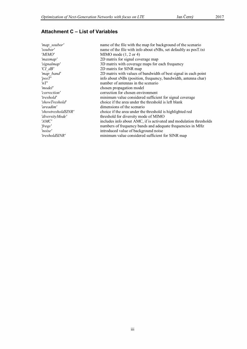
Optimization of Next-Generation Networks with focus on LTE Jan Černý 2017
iii
Attachment C – List of Variables
'map_soubor' name of the file with the map for background of the scenario 'soubor' name of the file with info about eNBs, set defaultly as posT.txt 'MIMO' MIMO mode (1, 2 or 4) 'maxmap' 2D matrix for signal coverage map 'signalmap' 3D matrix with coverage maps for each frequency 'CI_dB' 2D matrix for SINR map 'map_band' 2D matrix with values of bandwidth of best signal in each point 'posT' info about sNBs (position, frequency, bandwidth, antenna char) 'nT' number of antennas in the scenario 'model' chosen propagation model 'correction' correction for chosen environment 'treshold' minimum value considered sufficient for signal coverage 'showTreshold' choice if the area under the threshold is left blank 'areadim' dimensions of the scenario 'showtresholdSINR' choice if the area under the threshold is highlighted red 'diversityMode' threshold for diversity mode of MIMO 'AMC' includes info about AMC, if is activated and modulation thresholds 'freqs' numbers of frequency bands and adequate frequencies in MHz 'noise' introduced value of background noise 'tresholdSINR' minimum value considered sufficient for SINR map

Optimization of Next-Generation Networks with focus on LTE Jan Černý 2017
iv
Attachment D – MATLAB Code clc,clear %zadání vstupních hodnot function varargout = Simulation_LTE(varargin) % SIMULATION_LTE MATLAB code for Simulation_LTE.fig % Edit the above text to modify the response to help Simulation_LTE % Last Modified by GUIDE v2.5 26-Apr-2017 19:02:56 % Begin initialization code - DO NOT EDIT gui_Singleton = 1; gui_State = struct('gui_Name', mfilename, ... 'gui_Singleton', gui_Singleton, ... 'gui_OpeningFcn', @Simulation_LTE_OpeningFcn, ... 'gui_OutputFcn', @Simulation_LTE_OutputFcn, ... 'gui_LayoutFcn', [] , ... 'gui_Callback', []); if nargin && ischar(varargin{1}) gui_State.gui_Callback = str2func(varargin{1}); end if nargout [varargout{1:nargout}] = gui_mainfcn(gui_State, varargin{:}); else gui_mainfcn(gui_State, varargin{:}); end % End initialization code - DO NOT EDIT % --- Executes just before Simulation_LTE is made visible. function Simulation_LTE_OpeningFcn(hObject, eventdata, handles, varargin) % Choose default command line output for Simulation_LTE handles.output = hObject; % Update handles structure guidata(hObject, handles); %% inicialize structure of userdata with default values: s=struct('map_soubor','mapa4x5km.jpg',... 'soubor','posT.txt',... 'MIMO',2,... 'maxmap',0,... 'signalmap',0,... 'CI_dB',0,... 'map_band',0,... 'posT',0, ... 'nT',0, ... 'model',1,... 'correction',1,... 'treshold',-120,... 'showTreshold',0, ... 'areadim',[3000 4000], ... 'showtresholdSINR',0, ... 'diversityMode',4, ... 'AMC',[1 13 20], ... 'freqs',[1 2 3 4 5; 800 850 900 1800 2100], ... 'noise',-170, ... values of noise floor 'tresholdSINR',3); set(0,'showhiddenhandles','on'); myhandles = findobj('tag','figure1'); set(myhandles ,'userdata',s);

Optimization of Next-Generation Networks with focus on LTE Jan Černý 2017
v
ShowScenario_Callback(hObject, eventdata, handles) %% % --- Outputs from this function are returned to the command line. function varargout = Simulation_LTE_OutputFcn(hObject, eventdata, handles) varargout{1} = handles.output; function XX_Callback(hObject, eventdata, handles) myhandles = findobj('tag','figure1'); % loads handles of GUI s=get(myhandles ,'userdata'); % loads userdata from them s.areadim(2) = str2double(get(handles.XX, 'String')); % reads the value from GUI interface set(myhandles ,'userdata',s); % saves to handles % --- Executes during object creation, after setting all properties. function XX_CreateFcn(hObject, eventdata, handles) if ispc && isequal(get(hObject,'BackgroundColor'), get(0,'defaultUicontrolBackgroundColor')) set(hObject,'BackgroundColor','white'); end function YY_Callback(hObject, eventdata, handles) myhandles = findobj('tag','figure1'); % loads handles of GUI s=get(myhandles ,'userdata'); % loads userdata from them s.areadim(1) = str2double(get(handles.YY, 'String')); % reads the value from GUI interface set(myhandles ,'userdata',s); % saves to handles % --- Executes during object creation, after setting all properties. function YY_CreateFcn(hObject, eventdata, handles) if ispc && isequal(get(hObject,'BackgroundColor'), get(0,'defaultUicontrolBackgroundColor')) set(hObject,'BackgroundColor','white'); end function load_map_Callback(hObject, eventdata, handles) s.map_soubor = get(handles.load_map, 'String'); % reads the value from GUI interface set(myhandles ,'userdata',s); % saves to handles % --- Executes during object creation, after setting all properties. function load_map_CreateFcn(hObject, eventdata, handles) if ispc && isequal(get(hObject,'BackgroundColor'), get(0,'defaultUicontrolBackgroundColor')) set(hObject,'BackgroundColor','white'); end % --- Executes on selection change in model. function model_Callback(hObject, eventdata, handles) myhandles = findobj('tag','figure1'); % loads handles of GUI s=get(myhandles ,'userdata'); % loads userdata from them s.model = get(handles.model, 'Value'); % reads the value from GUI interface set(myhandles ,'userdata',s); % saves to handles
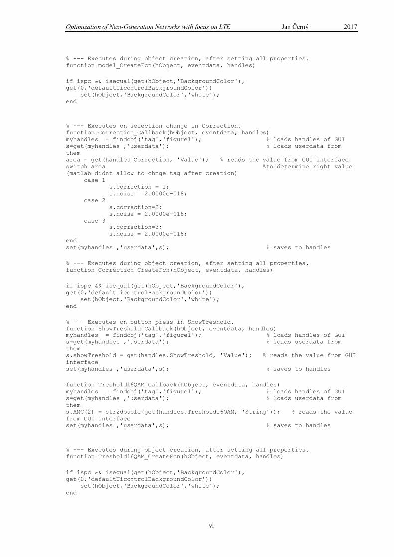
Optimization of Next-Generation Networks with focus on LTE Jan Černý 2017
vi
% --- Executes during object creation, after setting all properties. function model_CreateFcn(hObject, eventdata, handles) if ispc && isequal(get(hObject,'BackgroundColor'), get(0,'defaultUicontrolBackgroundColor')) set(hObject,'BackgroundColor','white'); end % --- Executes on selection change in Correction. function Correction_Callback(hObject, eventdata, handles) myhandles = findobj('tag','figure1'); % loads handles of GUI s=get(myhandles ,'userdata'); % loads userdata from them area = get(handles.Correction, 'Value'); % reads the value from GUI interface switch area %to determine right value (matlab didnt allow to chnge tag after creation) case 1 s.correction = 1; s.noise = 2.0000e-018; case 2 s.correction=2; s.noise = 2.0000e-018; case 3 s.correction=3; s.noise = 2.0000e-018; end set(myhandles ,'userdata',s); % saves to handles % --- Executes during object creation, after setting all properties. function Correction_CreateFcn(hObject, eventdata, handles) if ispc && isequal(get(hObject,'BackgroundColor'), get(0,'defaultUicontrolBackgroundColor')) set(hObject,'BackgroundColor','white'); end % --- Executes on button press in ShowTreshold. function ShowTreshold_Callback(hObject, eventdata, handles) myhandles = findobj('tag','figure1'); % loads handles of GUI s=get(myhandles ,'userdata'); % loads userdata from them s.showTreshold = get(handles.ShowTreshold, 'Value'); % reads the value from GUI interface set(myhandles ,'userdata',s); % saves to handles function Treshold16QAM_Callback(hObject, eventdata, handles) myhandles = findobj('tag','figure1'); % loads handles of GUI s=get(myhandles ,'userdata'); % loads userdata from them s.AMC(2) = str2double(get(handles.Treshold16QAM, 'String')); % reads the value from GUI interface set(myhandles ,'userdata',s); % saves to handles % --- Executes during object creation, after setting all properties. function Treshold16QAM_CreateFcn(hObject, eventdata, handles) if ispc && isequal(get(hObject,'BackgroundColor'), get(0,'defaultUicontrolBackgroundColor')) set(hObject,'BackgroundColor','white'); end

Optimization of Next-Generation Networks with focus on LTE Jan Černý 2017
vii
function Treshold_64QAM_Callback(hObject, eventdata, handles) myhandles = findobj('tag','figure1'); % loads handles of GUI s=get(myhandles ,'userdata'); % loads userdata from them s.AMC(3) = str2double(get(handles.Treshold_64QAM, 'String')); % reads the value from GUI interface set(myhandles ,'userdata',s); % saves to handles % --- Executes during object creation, after setting all properties. function Treshold_64QAM_CreateFcn(hObject, eventdata, handles) if ispc && isequal(get(hObject,'BackgroundColor'), get(0,'defaultUicontrolBackgroundColor')) set(hObject,'BackgroundColor','white'); end function Treshold_for_int_Callback(hObject, eventdata, handles) myhandles = findobj('tag','figure1'); % loads handles of GUI s=get(myhandles ,'userdata'); % loads userdata from them s.tresholdSINR = str2double(get(handles.Treshold_for_int, 'String')); % reads the value from GUI interface set(myhandles ,'userdata',s); % saves to handles % --- Executes during object creation, after setting all properties. function Treshold_for_int_CreateFcn(hObject, eventdata, handles) if ispc && isequal(get(hObject,'BackgroundColor'), get(0,'defaultUicontrolBackgroundColor')) set(hObject,'BackgroundColor','white'); end % --- Executes on button press in AMC_ON. function AMC_ON_Callback(hObject, eventdata, handles) myhandles = findobj('tag','figure1'); % loads handles of GUI s=get(myhandles ,'userdata'); % loads userdata from them s.AMC(1) = get(handles.AMC_ON, 'Value'); % reads the value from GUI interface set(myhandles ,'userdata',s); % saves to handles % --- Executes on button press in ShowInterf. function ShowInterf_Callback(hObject, eventdata, handles) myhandles = findobj('tag','figure1'); % loads handles of GUI s=get(myhandles ,'userdata'); % loads userdata from them s.showtresholdSINR = get(handles.ShowInterf, 'Value'); % reads the value from GUI interface set(myhandles ,'userdata',s); % saves to handles % --- Executes on button press in ShowScenario. function ShowScenario_Callback(hObject, eventdata, handles) myhandles = findobj('tag','figure1'); % loads handles of GUI s=get(myhandles ,'userdata'); % loads userdata from them img = imread(s.map_soubor); if (fopen(s.soubor,'r')<0); % if the file doesnt exist fclose('all'); else [s.posT,s.nT] = load_posT(s.soubor); % Loads positions and information about the eNBs from previous simulation end

Optimization of Next-Generation Networks with focus on LTE Jan Černý 2017
viii
axes(handles.axes1); cla title(''); plotBTS(s.areadim, s.nT,s.posT,s.freqs); % force axes orientation image(img); % Plot the image of map for orientation in the area plotBTS(s.areadim, s.nT,s.posT,s.freqs); % Plots positions of eNBs set(myhandles ,'userdata',s); % saves to handles % --- Executes on button press in Add_eNB. function Add_eNB_Callback(hObject, eventdata, handles) myhandles = findobj('tag','figure1'); % loads handles of GUI s=get(myhandles ,'userdata'); % loads userdata from them s.maxmap=0; s.signalmap=0; s.CI_dB=0; s.map_band=0; % free memory img = imread(s.map_soubor); axes(handles.axes1); title('Insert new eNB by rigt click'); addBTS(s.posT); % calls function for ading anothe eNB in the area title(''); [s.posT,s.nT] = load_posT(s.soubor); % reads modified list of eNBs axes(handles.axes1); cla plotBTS(s.areadim, s.nT,s.posT,s.freqs); % Plots positions of eNBs image(img); % Plot the image of map for orientation in the area plotBTS(s.areadim, s.nT,s.posT,s.freqs); % replots the scenario plotBTS(s.areadim, s.nT,s.posT,s.freqs); % Plots positions of eNBs set(myhandles ,'userdata',s); % saves to handles % --- Executes on button press in Edit_eNB. function Edit_eNB_Callback(hObject, eventdata, handles) myhandles = findobj('tag','figure1'); % loads handles of GUI s=get(myhandles ,'userdata'); % loads userdata from them s.maxmap=0; s.signalmap=0; s.CI_dB=0; s.map_band=0; % free memory if s.posT==0 % if scenario was not previously created msgbox('Nothing to edit'); else img = imread(s.map_soubor); axes(handles.axes1); title('Rigt click to area of a sector to edit it´s parameters'); editBTS(s.posT); % calls function to edit particular eNB (freq, Pmax) title(''); [s.posT,s.nT] = load_posT(s.soubor); % reads modified list of eNBs axes(handles.axes1); cla plotBTS(s.areadim, s.nT,s.posT,s.freqs); % Plots positions of eNBs image(img); % Plot the image of map for orientation in the area plotBTS(s.areadim, s.nT,s.posT,s.freqs); % replots the scenario end set(myhandles ,'userdata',s); % saves to handles % --- Executes on button press in Calc_coverage. function Calc_coverage_Callback(hObject, eventdata, handles) myhandles = findobj('tag','figure1'); % loads handles of GUI

Optimization of Next-Generation Networks with focus on LTE Jan Černý 2017
ix
s=get(myhandles ,'userdata'); % loads userdata from them if s.posT==0 % if scenario was not previously created msgbox('Create scenario first'); else s.maxmap=0; s.signalmap=0; s.CI_dB=0; s.map_band=0; % free memory %profile on [s.posT,s.nT] = load_posT(s.soubor); % reads list of eNBs s.signalmap=pokryti(s.posT, s.nT, s.areadim, s.model, s.correction, s.freqs); % calculates the coverage map and saves into signalmap.txt h = msgbox('Generating figure, please wait'); delete(findobj(h,'string','OK')); delete(findobj(h,'style','frame')); s.maxmap=MaxMap(s.areadim,s.signalmap); figure(12); cla plotBTS(s.areadim, s.nT,s.posT,s.freqs); % force axes orientation img = imread(s.map_soubor); %image(img); % Plot the image of map for orientation in the area showMap2(s.areadim, s.maxmap, s.posT, s.nT, s.showTreshold, s.treshold) % shows coverage map over the scenario plotBTS(s.areadim, s.nT,s.posT,s.freqs); title('Coverage map: maximum signal level [dBm]'); %coverage percentage covered=numel(find(s.maxmap>s.treshold)); % number of points covered with signal over treshold surface= s.areadim(1)* s.areadim(2); coverage=(covered/surface)*100 close(h) end %profile viewer %s set(myhandles ,'userdata',s); % saves to handles % --- Executes on button press in Delete_sector. function Delete_sector_Callback(hObject, eventdata, handles) myhandles = findobj('tag','figure1'); % loads handles of GUI s=get(myhandles ,'userdata'); % loads userdata from them s.maxmap=0; s.signalmap=0; s.CI_dB=0; s.map_band=0; % free memory if s.posT==0 % if scenario was not previously created msgbox('Noting to delete'); else axes(handles.axes1); title('Rigt click to area of an eNB you want to eliminate'); img = imread(s.map_soubor); deleteBTS(s.posT,s.nT); % calls functin for deleting eNB [s.posT,s.nT] = load_posT(s.soubor); % reads modified list of eNBs axes(handles.axes1); cla; title(''); plotBTS(s.areadim, s.nT,s.posT,s.freqs); % Plots positions of eNBs image(img); % Plot the image of map for orientation in the area plotBTS(s.areadim, s.nT,s.posT,s.freqs); end set(myhandles ,'userdata',s); % saves to handles % --- Executes on button press in Calc_Interferences. function Calc_Interferences_Callback(hObject, eventdata, handles) myhandles = findobj('tag','figure1'); % loads handles of GUI

Optimization of Next-Generation Networks with focus on LTE Jan Černý 2017
x
s=get(myhandles ,'userdata'); % loads userdata from them s.CI_dB=0; s.map_band=0; % free memory if s.signalmap==0 % if coverage was previously not calculated msgbox('Calculate coverage first'); else [s.CI_dB s.map_band] =calc_interference(s.signalmap, s.posT, s.freqs, s.noise, s.treshold); h = msgbox('Generating figure, please wait'); delete(findobj(h,'string','OK')); delete(findobj(h,'style','frame')); s.CI_dB(abs(s.CI_dB)==inf)=NaN; figure(21) cla %mesh(s.CI_dB); plotBTS(s.areadim, s.nT,s.posT,s.freqs); % force axes orientation img = imread(s.map_soubor); %image(img); % Plot the image of map for orientation in the area showMap2(s.areadim, s.CI_dB, s.posT, s.nT, s.showtresholdSINR, s.tresholdSINR) showMap2(s.areadim, s.CI_dB, s.posT, s.nT, s.showtresholdSINR, s.tresholdSINR) % shows coverage map over the scenario plotBTS(s.areadim, s.nT,s.posT,s.freqs); %view(2); if s.showtresholdSINR==0 title('SINR [dB]'); else % if chosen: [m,n]=find(s.CI_dB<s.tresholdSINR); % shows interferences in coverage map figure(21); plot(n,m,'. red'); title(strcat('SINR [dB], areas with SINR lower than ', num2str(s.tresholdSINR), ' dB marked red')); end % axis equal; close(h) end set(myhandles ,'userdata',s); % saves to handles % --- Executes on button press in radiobutton1. function radiobutton1_Callback(hObject, eventdata, handles) % --- If Enable == 'on', executes on mouse press in 5 pixel border. % --- Otherwise, executes on mouse press in 5 pixel border or over radiobutton1. function radiobutton1_ButtonDownFcn(hObject, eventdata, handles) % --- Executes on button press in CloseSimulation. function CloseSimulation_Callback(hObject, eventdata, handles) clear close all % --- Executes when selected object is changed in uipanel1. function uipanel1_SelectionChangeFcn(hObject, eventdata, handles) myhandles = findobj('tag','figure1'); % loads handles of GUI s=get(myhandles ,'userdata'); % loads userdata from them mimo = get(eventdata.NewValue, 'Tag'); % reads the value from GUI interface switch mimo %to determine right value (matlab didnt allow to chnge tag after creation) case 'mimoOFF'
Optimization of Next-Generation Networks with focus on LTE Jan Černý 2017
xi
s.MIMO=1; case 'mimo2' s.MIMO=2; case 'mimo4' s.MIMO=4; end %whos s.MIMO set(myhandles ,'userdata',s); % saves to handles % --- Executes during object creation, after setting all properties. function axes1_CreateFcn(hObject, eventdata, handles) % --- Executes on button press in Data_Troughput. function Data_Troughput_Callback(hObject, eventdata, handles) myhandles = findobj('tag','figure1'); % loads handles of GUI s=get(myhandles ,'userdata'); % loads userdata from them if s.CI_dB==0 % if coverage was previously not calculated msgbox('Calculate interference first'); else %maxmap=MaxMap(areadim,signalmap_lin); h = msgbox('Generating figure, please wait'); delete(findobj(h,'string','OK')); delete(findobj(h,'style','frame')); lteSpeed=LTE_speed(s.CI_dB, s.maxmap, s.treshold, s.map_band, s.MIMO, s.AMC,s.diversityMode); figure(23) %plotBTS(s.areadim, s.nT,s.posT,s.freqs); % force axes orientation img = imread(s.map_soubor); cla plotBTS(s.areadim, s.nT,s.posT,s.freqs); % force axes orientation %image(img); % Plot the image of map for orientation in the area showMap2(s.areadim, lteSpeed, s.posT, s.nT, 0, 0) %mesh(lteSpeed); plotBTS(s.areadim, s.nT,s.posT,s.freqs); %view(2); %axis equal; title('Throughput of LTE network [Mbps]'); % colorbar close(h) end set(myhandles ,'userdata',s); % saves to handles function Treshold_Callback(hObject, eventdata, handles) myhandles = findobj('tag','figure1'); % loads handles of GUI s=get(myhandles ,'userdata'); % loads userdata from them s.treshold = str2double(get(handles.Treshold, 'String')); % reads the value from GUI interface set(myhandles ,'userdata',s); % saves to handles % --- Executes during object creation, after setting all properties. function Treshold_CreateFcn(hObject, eventdata, handles) if ispc && isequal(get(hObject,'BackgroundColor'), get(0,'defaultUicontrolBackgroundColor')) set(hObject,'BackgroundColor','white'); end % --- Executes on button press in OpenMap. function OpenMap_Callback(hObject, eventdata, handles) myhandles = findobj('tag','figure1'); % loads handles of GUI

Optimization of Next-Generation Networks with focus on LTE Jan Černý 2017
xii
s=get(myhandles ,'userdata'); % loads userdata from them [s.map_soubor,PathName] = uigetfile('*.jpg','Select the MATLAB code file'); set(myhandles ,'userdata',s); % saves to handles function edit8_Callback(hObject, eventdata, handles) myhandles = findobj('tag','figure1'); % loads handles of GUI s=get(myhandles ,'userdata'); % loads userdata from them s.areadim(2) = str2double(get(handles.XX, 'String')); % reads the value from GUI interface set(myhandles ,'userdata',s); % saves to handles % --- Executes during object creation, after setting all properties. function edit8_CreateFcn(hObject, eventdata, handles) if ispc && isequal(get(hObject,'BackgroundColor'), get(0,'defaultUicontrolBackgroundColor')) set(hObject,'BackgroundColor','white'); end function DiversityMode_Callback(hObject, eventdata, handles) % treshold for diversity MIMO mode myhandles = findobj('tag','figure1'); % loads handles of GUI s=get(myhandles ,'userdata'); % loads userdata from them s.diversityMode = str2double(get(handles.DiversityMode, 'String')); % reads the value from GUI interface set(myhandles ,'userdata',s); % saves to handles % --- Executes during object creation, after setting all properties. function DiversityMode_CreateFcn(hObject, eventdata, handles) if ispc && isequal(get(hObject,'BackgroundColor'), get(0,'defaultUicontrolBackgroundColor')) set(hObject,'BackgroundColor','white'); end function BG_noise_Callback(hObject, eventdata, handles) myhandles = findobj('tag','figure1'); % loads handles of GUI s=get(myhandles ,'userdata'); % loads userdata from them s.bg_noise = str2double(get(handles.BG_noise, 'String')); % reads the value from GUI interface set(myhandles ,'userdata',s); % saves to handles % --- Executes during object creation, after setting all properties. function BG_noise_CreateFcn(hObject, eventdata, handles) if ispc && isequal(get(hObject,'BackgroundColor'), get(0,'defaultUicontrolBackgroundColor')) set(hObject,'BackgroundColor','white'); end % --- Executes on button press in Reset. function Reset_Callback(hObject, eventdata, handles) % in case program ends incorrectly fclose all; % and on another run gives "badly formated string" error delete posT.txt close all

Optimization of Next-Generation Networks with focus on LTE Jan Černý 2017
xiii
clear all; clc; function [posT, nT] = deleteBTS(posT,nT) % deleteBTS deletes chosen BTS (closest to where click is made) if (nT==3) % if there is only one BTS delete all file to prevent error of badly formated string delete('posT.txt') nT=0; end if (fopen('posT.txt','r+')<0); %if the file doesn´t exist - do nothing else index=pickCell(posT); % find the nearest BTS, meaning BTS of the desired cell % finds other 3 sector BTS of the eNB: sector= posT(index, 5); start=index-sector+1; % first sector of choosen eNB before=posT(1:start-1,:); % posT before deleted eNB after=posT(start+3:nT,:); % posT after deleted eNB posT=[before; after]; nT=size(posT,1); dlmwrite('posT.txt',posT,'\t'); % save to file fclose('all'); end end function [posT,nT] = addBTS(oldposT) % addBTS place new BTS to simulation %% adding BTS [A,B]=getpts(); % generate new position of the BS from clicking on previous graph X=A(1); Y=B(1); % takes position only of the first click %n_ant = choose_ant_number; % calls selection of number of antennas (3 or 6) n_ant=3; for ii=1:n_ant % always places 3 sektors global power sirka vyska dir Dir band nf Dir=ii; %goes to gui for antenna settings to rotate the dirrection is the antenna poining shift=2; if Dir>3 % for case of 6 antenas (soft reuse) Dir=Dir-3; % dirrection of antenna repeats shift=4; %shift antenna position more end f=eNB_table; % calling gui for introducing parameters of the transmiter uiwait(f) % waits for the window to be closed %-------------------------------------------------------------------- switch Dir % shifts antennas one pixel (resp 2ú so the dont overlaps case 1 Yant = Y-shift; Xant = X-shift; case 2 Yant = Y+shift; Xant = X; case 3 Yant = Y-shift; Xant = X+shift; end %---------------------------------------------------------------------- newposT=[Yant, Xant, nf, power, Dir, sirka, vyska, band]; % ector of info about at to be saved to the posT.txt if (oldposT==0) % if thereareno previous data
Optimization of Next-Generation Networks with focus on LTE Jan Černý 2017
xiv
posT=newposT; % only take the the new data else posT=[oldposT;newposT]; % connect loaded and imputted position matrixes end nT=size(posT); oldposT=posT; end %saving data dlmwrite('posT.txt',posT,'\t'); % save to file fclose('all'); end function posT = editBTS(posT) % editBTS edit values of chosen BTS (closest to where click is introduced) if (fopen('posT.txt','r+')<0); %if the file doesn´t exist - do nothing else index=pickCell(posT); % find the nearest BTS, meaning BTS of the desired cell global power sirka vyska Dir band nf sector=posT(index,5); % reads sector of edited antenna power=posT(index,4); % reads sector of edited antenna nf=posT(index,3); % reads sector of edited antenna band=posT(index,8); % reads sector of edited antenna Dir=sector; % to show the edited antenna characteristic correctly oriented %--------------------------------------GUI-------------------- f=eNB_table; % calls gui to change antenna uiwait(f) % waits for the gui window to be closed %------------------------------------------------------------- posT(index,3:8) = [nf, power, sector, sirka, vyska, band]; % place introduced new data into the table of BTS % saving data dlmwrite('posT.txt',posT,'\t'); % save to file fclose('all'); end end function [posT,nT] = load_posT(soubor) % inicializeBTS read saved positions of BTSes %soubor='posT.txt' if (fopen(soubor,'r')<0); % if the file doesnt exist fopen(soubor,'w+'); posT=0; nT=0; else % if the fiele does exist posT=dlmread(soubor); % we reads saved BS nT=size(posT); nT=nT(1); % number of loaded BS end; fclose('all'); end function index = pickCell(posT) [A,B]=getpts(); Y=round(A(1)); X=round(B(1)); %pickcell=[X,Y]; x=posT(:,1); % x coordiantes of all eNBs y=posT(:,2); % y coordiantes of all eNBs %x1=pickcell(1); % coordinates of picked cell %y1=pickcell(2); dist=sqrt((x-X).^2+(y-Y).^2); index=find(dist==min(min(dist))); % find the nearest BS, meaning BS of the desired cell

Optimization of Next-Generation Networks with focus on LTE Jan Černý 2017
xv
function s = plotBTS(areadim,nT,posT,freqs) % plot positions of BTS, their name and freq. % plot(XV,YV,'k--') % replot the hexagonal network eNB=0; % počítá vykreslené eNB a číslujeje axis equal XX=areadim(1); YY=areadim(2); axis([0 YY 0 XX]) zoom on xlabel('x [m]') ylabel('y [m]') hold on if (nT>0) % process only if there is something to process for ii=1:nT % loop to plot every BS if (rem(ii,3)==1) % pro každou tři+první eNB eNB=eNB+1; if (0<posT(ii,1) && posT(ii,1)<XX && 0<posT(ii,2)&& posT(ii,2)<YY) % only if BTS is inside plotted field x=posT(ii,2); % coordinates of eNB y=posT(ii,1); d=100; % lengt of the lines of cross plot([x-d x x x x+d],[y+d y y-d y y+d],'k') % plots cross defining sectors plot(x,y,'O',x,y,'*') % plots the eNB name = strcat(' eNB ',num2str(eNB)); % prepare strings with information aout eNB and sectors sect1 = sprintf('S1: %d dBm\n%d MHz \n%.2f MHz .', posT(ii,4), freqs(2,posT(ii,3)),posT(ii,8)); sect2 = sprintf('S2: %d dBm\n%d MHz \n%.2f MHz .', posT(ii+1,4), freqs(2,posT(ii+1,3)),posT(ii+1,8)); sect3 = sprintf('S3: %d dBm\n%d MHz \n%.2f MHz .', posT(ii+2,4), freqs(2,posT(ii+2,3)),posT(ii+2,8)); text(posT(ii,2)+35,posT(ii,1)+4,name) % plotting the strings text(posT(ii,2)-650,posT(ii,1)-250,sect1) text(posT(ii,2)-150,posT(ii,1)+300,sect2) text(posT(ii,2)+100,posT(ii,1)-250,sect3) end end end end end function varargout = eNB_table(varargin) gui_Singleton = 1; gui_State = struct('gui_Name', mfilename, ... 'gui_Singleton', gui_Singleton, ... 'gui_OpeningFcn', @eNB_table_OpeningFcn, ... 'gui_OutputFcn', @eNB_table_OutputFcn, ... 'gui_LayoutFcn', [] , ... 'gui_Callback', []); if nargin && ischar(varargin{1}) gui_State.gui_Callback = str2func(varargin{1}); end if nargout

Optimization of Next-Generation Networks with focus on LTE Jan Černý 2017
xvi
[varargout{1:nargout}] = gui_mainfcn(gui_State, varargin{:}); else gui_mainfcn(gui_State, varargin{:}); end % --- Executes just before eNB_table is made visible. function eNB_table_OpeningFcn(hObject, eventdata, handles, varargin) handles.output = hObject; guidata(hObject, handles); %% initial data for char of antenna graph and default values of the query: global power sirka vyska dir Dir uhel uhelRad band nf power=30; %transmited power in mW nf=1; % number of freq band band=15; % bandwidth in MHz sirka=0.76; %nastavuje šířku paprsku vyska=2; %nastavuje směrovost %dir=0; %uhel vyzařování dir=Dir*120-240; % dle vybraneho sektoru nastavi uhel uhel=-180:0.1:180; %osa x (uhel) uhelRad=uhel*pi/180; %% ploting characteristic ---------------------------------------------------------------------- dirRad=dir*pi/180; %přepočet na radiany Char=(sinc(sirka*uhelRad-sirka*dirRad)).^vyska; %funkce pro aproximaci charakteristiky anteny [U]=((Char)<(0.048)); Char(U)=0; % zmenšení vedlejších laloků fun=@(uhel) ((sinc(sirka*uhel-sirka*dirRad)).^vyska); %definice funkce pro integraci omnidir=abs(abs(quad(fun,-180,180)))/360; %integral z funkce/2Pí = char omnidirekcionální anteny ChardB=((10*log10(Char/omnidir))); %zisk antény (vstaženo na všesměrovou) ChardB(ChardB<0)=0; %ořízne hluboké zářezy charakteristiky polar(uhelRad,ChardB)% polarní v dB view([90 -90]) % rotating the graph to align with simulation result %% --------------------------------------------------------------------------------------------- % UIWAIT makes eNB_table wait for user response (see UIRESUME) % uiwait(handles.figure1); % --- Outputs from this function are returned to the command line. function varargout = eNB_table_OutputFcn(hObject, eventdata, handles) % varargout cell array for returning output args (see VARARGOUT); % hObject handle to figure % eventdata reserved - to be defined in a future version of MATLAB % handles structure with handles and user data (see GUIDATA) % Get default command line output from handles structure varargout{1} = handles.output; % --- Executes on button press in OK_button. function OK_button_Callback(hObject, eventdata, handles) close eNB_table % --- Executes on change function Power_Callback(hObject, eventdata, handles)

Optimization of Next-Generation Networks with focus on LTE Jan Černý 2017
xvii
global power power=str2num(get(handles.Power,'String')); % --- Executes during object creation, after setting all properties. function Power_CreateFcn(hObject, eventdata, handles) if ispc && isequal(get(hObject,'BackgroundColor'), get(0,'defaultUicontrolBackgroundColor')) set(hObject,'BackgroundColor','white'); end % --- Executes on selection change in chooseFreq. function chooseFreq_Callback(hObject, eventdata, handles) global nf; %number of band (goes to saved file posT) nf=get(handles.chooseFreq,'Value'); function chooseFreq_CreateFcn(hObject, eventdata, handles) if ispc && isequal(get(hObject,'BackgroundColor'), get(0,'defaultUicontrolBackgroundColor')) set(hObject,'BackgroundColor','white'); end % --- Executes on slider movement. function Uhel_Callback(hObject, eventdata, handles) %% initial data for char of antenna graph: global sirka vyska dir uhel uhelRad dir=(get(handles.Uhel,'Value'))*240-120 % returns position of slider %% ploting characteristic ---------------------------------------------------------------------- dirRad=dir*pi/180; %přepočet na radiany Char=(sinc(sirka*uhelRad-sirka*dirRad)).^vyska; %funkce pro aproximaci charakteristiky anteny fun=@(uhel) ((sinc(sirka*uhel-sirka*dirRad)).^vyska); %definice funkce pro integraci omnidir=abs(quad(fun,-180,180))/360 %integral z funkce/2Pí = char omnidirekcionální anteny ChardB=((10*log10(Char/omnidir))); %zisk antény (vstaženo na všesměrovou) ChardB(ChardB<0)=0; %ořízne hluboké zářezy charakteristiky polar(uhelRad,ChardB)% polarní v dB view([90 -90]) % rotating the graph to align with simulation result %% % --- Executes during object creation, after setting all properties. function Uhel_CreateFcn(hObject, eventdata, handles) if isequal(get(hObject,'BackgroundColor'), get(0,'defaultUicontrolBackgroundColor')) set(hObject,'BackgroundColor',[.9 .9 .9]); end % --- Executes on slider movement. function Vyska_Callback(hObject, eventdata, handles) %% initial data for char of antenna graph: global sirka vyska dir uhel uhelRad vyska=((get(handles.Vyska,'Value'))*2)+1 %returns position of slider from 1 to 3 %% ploting characteristic ---------------------------------------------------------------------- dirRad=dir*pi/180; %přepočet na radiany

Optimization of Next-Generation Networks with focus on LTE Jan Černý 2017
xviii
Char=(sinc(sirka*uhelRad-sirka*dirRad)).^vyska; %funkce pro aproximaci charakteristiky anteny fun=@(uhel) ((sinc(sirka*uhel-sirka*dirRad)).^vyska); %definice funkce pro integraci omnidir=abs(quad(fun,-180,180))/360 %integral z funkce/2Pí = char omnidirekcionální anteny ChardB=((10*log10(Char/omnidir))); %zisk antény (vstaženo na všesměrovou) ChardB(ChardB<0)=0; %ořízne hluboké zářezy charakteristiky polar(uhelRad,ChardB)% polarní v dB view([90 -90]) % rotating the graph to align with simulation result %% % --- Executes during object creation, after setting all properties. function Vyska_CreateFcn(hObject, eventdata, handles) if isequal(get(hObject,'BackgroundColor'), get(0,'defaultUicontrolBackgroundColor')) set(hObject,'BackgroundColor',[.9 .9 .9]); end % --- Executes on slider movement. function Sirka_Callback(hObject, eventdata, handles) %% initial data for char of antenna graph: global sirka vyska dir uhel uhelRad sirka=(get(handles.Sirka,'Value'))*2 %returns position of slider %% ploting characteristic ---------------------------------------------------------------------- dirRad=dir*pi/180; %přepočet na radiany Char=(sinc(sirka*uhelRad-sirka*dirRad)).^vyska; %funkce pro aproximaci charakteristiky anteny fun=@(uhel) ((sinc(sirka*uhel-sirka*dirRad)).^vyska); %definice funkce pro integraci omnidir=abs(quad(fun,-180,180))/360 %integral z funkce/2Pí = char omnidirekcionální anteny ChardB=((10*log10(Char/omnidir))); %zisk antény (vstaženo na všesměrovou) ChardB(ChardB<0)=0; %ořízne hluboké zářezy charakteristiky polar(uhelRad,ChardB)% polarní v dB view([90 -90]) % rotating the graph to align with simulation result %% % --- Executes during object creation, after setting all properties. function Sirka_CreateFcn(hObject, eventdata, handles) % hObject handle to Sirka (see GCBO) % eventdata reserved - to be defined in a future version of MATLAB % handles empty - handles not created until after all CreateFcns called % Hint: slider controls usually have a light gray background. if isequal(get(hObject,'BackgroundColor'), get(0,'defaultUicontrolBackgroundColor')) set(hObject,'BackgroundColor',[.9 .9 .9]); end % --- Executes on selection change in Band. function Band_Callback(hObject, eventdata, handles) global band; n_band=(get(handles.Band,'Value')); % we get number of selection option=[15 1.25 2.5 5 10 15 20 ]; band=option(n_band); % picks adequate band accoarding to selection % --- Executes during object creation, after setting all properties. function Band_CreateFcn(hObject, eventdata, handles) if ispc && isequal(get(hObject,'BackgroundColor'), get(0,'defaultUicontrolBackgroundColor')) set(hObject,'BackgroundColor','white'); end

Optimization of Next-Generation Networks with focus on LTE Jan Černý 2017
xix
function maxmap = MaxMap(areadim, signalmap) %calculates maximums of signal XX=areadim(2); YY=areadim(1); % calculating map of maximum values maxmap=zeros(YY,XX,'single'); maxmap=max(signalmap,[],3); % maximum velue on each point maxmap(maxmap<-150)=-150; % sets limit because of graphical representation maxmap(1,1)=-150; % tu uniform colours, LTE % is defined to -140 end %% function to calculate level of signal from one transmitter function [signalmap] = cost(posT, index, areadim, correction, freqs) sektor=posT(index,5); number_of_freq_band=posT(index,3); % reads number of frq band of this transmiter fc=freqs(2, number_of_freq_band); % finds asigned frequency) XX=areadim(2); YY=areadim(1); xx=posT(index,2); yy=posT(index,1); %% parameters of signal spreading (Cost231 - hata model for cities) Pv=posT(index,4); % Power of BTS hb = 30; hm = 2; %% Correction for enviroment switch correction case 1 % city Cm = 3; case 2 % sub urban Cm = 0; case 3 % open areas Cm = 0; end %% calculate signal level for each point mapdist=sektDist2(areadim, posT, index); a = (1.1*log10(fc)-0.7)*hm - (1.56*log10(fc) - 0.8); %correction factor L = 46.3 +33.9*log10(fc) - 13.82*log10(hb) - a + (44.9 - 6.55*log10(hb))*log10(mapdist/1000)+Cm; %% směrovost sirka=posT(index,6); %sirka charakteristiky anteny vyska=posT(index,7); dir=sektor*120-240; % dle vybraneho sektoru nastavi uhel dirRad=dir*pi/180; % přepočte na rad [X,Y] = meshgrid(0:1:XX-1, 0:1:YY-1); % vytvoří mesh (hodnota=souřadnice) mapAngRad=(atan2(X-xx,Y-yy)); % vypočítá uhel (azimut) Theta mapChar=(sinc(sirka*mapAngRad-sirka*dirRad)).^vyska; %mapChar=(sin(mapAngRad+dirRad)); % charakteristika v závislosti na uhlu Theta %mapChar(mapChar<0)=0;%1e-15; % %mapChar(((mapChar))<(0.048))=0; [laloky]=((mapChar)<(0.048)); mapChar(laloky)=10e-30;%abs(mapChar(laloky)./5); % zmenšení vedlejších lalok? % figure % mesh(mapChar) % view(2) % axis equal signalmapcharLin=mapChar.*10.^((Pv-L)./10); signalmap=10*log10(signalmapcharLin); end

Optimization of Next-Generation Networks with focus on LTE Jan Černý 2017
xx
%% function to calculate level of signal from one transmitter function [signalmap] = OkumuraHata(posT, index, areadim, correction, freqs) sektor=posT(index,5); number_of_freq_band=posT(index,3); % reads number of frq band of this transmiter fc=freqs(2, number_of_freq_band); % finds asigned frequency) XX=areadim(2); YY=areadim(1); xx=posT(index,2); yy=posT(index,1); %% parameters of signal spreading (Cost231 - hata model for cities) Pv=posT(index,4); % Power of BTS hb = 30; hm = 2; %% Correction for enviroment switch correction case 1 % city Kr = 0; case 2 % sub urban Kr = 2*(log10(fc/28))^2 + 5.4; case 3 % open areas Kr = 4.78*(log10(fc))^2 - 18.33 * log10(fc) + 40.94 end %% calculate signal level for each point mapdist=sektDist2(areadim, posT, index); a = 3.2*(log10(11.75*hm))^2 - 4.97; % correction factor L = 69.55 + 26.16*log10(fc) - 13.82*log10(hb) - a + (44.9 - 6.55*log10(hb))*log10(mapdist/1000)-Kr; %% směrovost sirka=posT(index,6); %sirka charakteristiky anteny vyska=posT(index,7); dir=sektor*120-240; % dle vybraneho sektoru nastavi uhel dirRad=dir*pi/180; % přepočte na rad [X,Y] = meshgrid(0:1:XX-1, 0:1:YY-1); % vytvoří mesh (hodnota=souřadnice) mapAngRad=(atan2(X-xx,Y-yy)); % vypočítá uhel (azimut) Theta mapChar=(sinc(sirka*mapAngRad-sirka*dirRad)).^vyska; [laloky]=((mapChar)<(0.048)); mapChar(laloky)=0;%abs(mapChar(laloky)./5); % zmenšení vedlejších lalok? signalmapcharLin=mapChar.*10.^((Pv-L)./10); signalmap=10*log10(signalmapcharLin); end function signalmap = pokryti(posT,nT,areadim, model, correction, freqs) %calcualte coverage map acoarding to chosen model XX=areadim(2); YY=areadim(1); signalmap=zeros(YY,XX,nT,'single');%,'single'); % mapy pokrytí od jednotivých vysílačů if (nT>0) % process only if there is something to process switch model % choose model to calculate the coverage case 1 h=waitbar(0,'Calculating the coverage. Please wait...'); % show teps of calculation hw=findobj(h,'Type','Patch'); set(hw,'EdgeColor',[0 1 0],'FaceColor',[0 1 0]) % changes the color to green for ii=1:nT

Optimization of Next-Generation Networks with focus on LTE Jan Černý 2017
xxi
signalmap(:,:,ii)=cost(posT, ii, areadim, correction,freqs); waitbar(ii/nT) %updates bar end; close(h) case 2 h=waitbar(0,'Calculating the coverage. Please wait...'); % show teps of calculation hw=findobj(h,'Type','Patch'); set(hw,'EdgeColor',[0 1 0],'FaceColor',[0 1 0]) % changes the color to green for ii=1:nT signalmap(:,:,ii)=OkumuraHata(posT, ii, areadim, correction,freqs); waitbar(ii/nT) %updates bar end; close(h) end else signalmap=0; end end function [ mapdist ] = sektDist(areadim, posT, index ) %SEKTDIST calculates distance from BTS to calculate coverage. % Takes in account sectorization and calculate nonzero values only in area % of given sector % %% sectorization %a=0; asi se da vymazat %fi0=a; fi1=a+120; fi2=a+240; xx=posT(index,1); yy=posT(index,2); %sektor=posT(index,5); %% distance calculation XX=areadim(2); YY=areadim(1); mapdist=zeros(YY,XX); %generates matriq of adequal dim. for ii=1:XX, for jj=1:YY, mapdist(jj,ii)=sqrt((ii-yy).^2+(jj-xx).^2); end end [y0,x0]=find(mapdist<30); % locate if distance less than 30 mapdist(y0,x0)=30; % change distance to 30 to avoid peaks - used modelas are not valid for this distance anyway end function s = showMap(areadim,maxmap,posT,nT,showTreshold, treshold) % present calculated coverage map (maxmap) XX=areadim(1); YY=areadim(2); axis equal axis([0 YY 0 XX]) zoom on xlabel('x [m]') ylabel('y [m]') if (showTreshold==1) % pokud je požadováno, zbarví se oblasti s nedostatečným signálem maxmap(maxmap<treshold)=NaN; end imagescwithnan(maxmap,jet,[1 1 1]); % plots the maxmap

Optimization of Next-Generation Networks with focus on LTE Jan Černý 2017
xxii
axis equal axis([0 YY 0 XX]) % axes zoom on xlabel('x [m]') ylabel('y [m]') hold on colorbar end %% function to calculate CIR function [CImap map_band] = calc_interference(signalmap, posT, freqs, bg_noise,treshold) %----------- waitbar -------- h=waitbar(0,strcat('Calculating the interference. Please wait...')); % show teps of calculation hw=findobj(h,'Type','Patch'); set(hw,'EdgeColor',[0 1 0],'FaceColor',[0 1 0]) % changes the color to green fmap=zeros(XX,YY,nT); %----------- waitbar -------- [XX YY nT]=size(signalmap); % recovery of dimesions nf=length(freqs); % number of frequencies used in network nf_used=numel(unique(posT(:,3))); % number of used frequencies in the scenario CImap3d=zeros(XX,YY,nf_used,'int16'); % memory alocation map_band3d=zeros(XX,YY,nf,'int8'); map_band=zeros(XX,YY,'int8'); for ff=1:nf; % goes over all possible frequency bands nVysilac=0; % counts number of transmitters with given frequency vysilacu=numel(find(ff==posT(:,3))); % how many transmitters of this frequency appear if vysilacu>0 % if this frequency is used in the simulation fmap=zeros(XX,YY,vysilacu,'single'); posT_fmap=zeros(vysilacu,8); % info about transmiters of this freq for ii=1:nT if(posT(ii,3)==ff) % frekvence ii-tého vysílače odpovídá frekvenci hledané (ff) nVysilac=nVysilac+1; % counts them fmap(:,:,nVysilac)=(signalmap(:,:,ii));% add covermap with adecuate frequency posT_fmap(nVysilac,:)= posT(ii,:); % reorganise info about antennas to match fmap end end [carrier posMax]=max(fmap,[],3); % first maximum on the same freq vectB=posT_fmap(:,8); Bmap_pom=vectB(posMax); % matching map of bandwidth map_band3d(:,:,ff)=Bmap_pom; % saves it on side of bmaps for other freqs [m,n,o] = size(fmap); % generates indexes of found maximum dim1 = mod((0:m*n-1)', m)+1; dim2 = ceil((1:m*n)/m)'; dim3 = posMax(:); position = sub2ind(size(fmap), dim1, dim2, dim3); position = reshape(position, m, n, 1);

Optimization of Next-Generation Networks with focus on LTE Jan Černý 2017
xxiii
fmap(position)=-inf; % sets value on positions of previous maximums to -infinity interf=max(fmap,[],3); % find second maximum rec_noise=bg_noise + 10*log10(Bmap_pom); % calculates noise for each point interf(interf<rec_noise)=rec_noise(interf<rec_noise); % if there is no interf. signal - noise is the interference singnal carrier(carrier<treshold)=NaN; % if there is no signal -> there is NaN signal CImap3d(:,:,ff)=carrier-interf; % calculate CIR itself for each freq end waitbar(ff/nf); %updates waitbar end [CImap ind]=max(CImap3d,[],3); % gets maximum SNIR for each point and position % replicates indexes in other dimensions [m,n,o] = size(CImap3d); dim1 = mod((0:m*n-1)', m)+1; dim2 = ceil((1:m*n)/m)'; dim3 = ind(:); position = sub2ind(size(CImap3d), dim1, dim2, dim3); position = reshape(position, m, n, 1); map_band=map_band3d(position); % puts adequate bandwidths on positions of found max SNIR close(h) end function [ speed_map ] = LTE_speed(CI_dB, maxmap, treshold, map_band, MIMO, AMC, diversityMode) [XX YY]=size(maxmap); % obnovení rozměrů oblasti speed_map=zeros(XX,YY,'single'); % alokace map_band=single(map_band); %PRBs = (15 * 5)% / 1000000; % dle http://www.radio-electronics.com/info/cellulartelecomms/lte-long-term-evolution/lte-ofdm-ofdma-scfdma.php symbols_per_carrier = 7; % pro shor cyclyc prefix a 6 pro long CP for ii=1:XX for jj=1:YY MIMO_mode=MIMO; SINR=CI_dB(ii,jj); % odstup signalu od šumu pro daný bod signal=maxmap(ii,jj); % uroven signalu v tomto bodě if (AMC(1) == 1) % pokud je aktivována adaptivní modulace závisí počet bitů na symbol na SINR if ((SINR==-Inf)||(signal<treshold)) % pokud není udaj o interferencích nebo není signal dostatečný modulace = -inf; % znamená že není signál - rychlost bude NaN else if (SINR<AMC(2)) modulace = 2; % QPSK end if (AMC(3)>SINR && SINR>AMC(2)) modulace = 4; % 16QAM end if (SINR>AMC(3)) modulace = 6; % 64QAM end
Optimization of Next-Generation Networks with focus on LTE Jan Černý 2017
xxiv
end else modulace = 2; end if (SINR<diversityMode) % under treshold for diversity mode switchs MIMO to diversity mode MIMO_mode = 1; % diversity mode end B=map_band(ii,jj); % recover information aboud f band i this point PRBs = (B * 5); % dle http://www.radio-electronics.com/info/cellulartelecomms/lte-long-term-evolution/lte-ofdm-ofdma-scfdma.php speed_map(ii,jj) = (modulace * PRBs * 12 * symbols_per_carrier * 2000 * MIMO_mode)/1000000; % PRBs x subcarriers x symbols per subcarier x (1/čas timeslotu) x bit/symbol dle modulace x MIMO end end speed_map(abs(speed_map)==inf)=NaN; speed_map((speed_map)==0)=NaN; % porcentage of max speed coverage: maxspeed=numel(find(speed_map==max(max(speed_map)))); %maxspeed=numel(find(speed_map<30)); surface=XX*YY; max_speed_coverage=(maxspeed/surface)*100 end function [h hcb] = imagescwithnan(a,cm,nanclr) % %from http://stackoverflow.com/questions/8481324/contrasting-color-for-nans-in- imagesc % IMAGESC with NaNs assigning a specific color to NaNs %# find minimum and maximum amin=min(a(:))-1; amax=max(a(:)); %# size of colormap n = size(cm,1); %# color step dmap=(amax-amin)/n; %# standard imagesc him = imagesc(a); %# add nan color to colormap colormap([nanclr; cm]); %# changing color limits caxis([amin-dmap amax]); %# place a colorbar hcb = colorbar; %# change Y limit for colorbar to avoid showing NaN color ylim(hcb,[amin amax]) if nargout > 0 h = him; end

Optimization of Next-Generation Networks with focus on LTE Jan Černý 2017
xxv
Attachment E – Optimized Scenario
2792.9 4467.4 1 25 1 0.76 2 5 2796.9 4469.4 2 25 2 0.76 2 5 2792.9 4471.4 3 25 3 0.76 2 5 684.29 2425.1 1 25 1 0.76 2 5 688.29 2427.1 2 25 2 0.76 2 5 684.29 2429.1 3 25 3 0.76 2 5 2702.3 7696.9 1 25 1 0.76 2 15 2706.3 7698.9 1 25 2 0.76 2 15 2702.3 7700.9 1 25 3 0.76 2 15 465.74 6159.3 1 25 1 0.76 2 5 469.74 6161.3 2 25 2 0.76 2 5 465.74 6163.3 3 25 3 0.76 2 5 5057.1 6385.1 1 25 1 0.76 2 5 5061.1 6387.1 2 25 2 0.76 2 5 5057.1 6389.1 3 25 3 0.76 2 5 4220.9 1665.8 1 30 1 0.76 2 5 4224.9 1667.8 2 30 2 0.76 2 5 4220.9 1669.8 3 30 3 0.76 2 5