diplomarbeit - tbi · diplomarbeit strategies for measuring evolutionary conservation of rna...
TRANSCRIPT

DIPLOMARBEIT
Strategies for measuring evolutionary
conservation of RNA secondary structures
angestrebter akademischer Grad
Magister der Naturwissenschaften (Mag. rer. nat.)
Verfasser: Andreas Gruber
Matrikelnummer: 0008234
Studienrichtung: Molekulare Biologie
Betreuer: Ao. Univ.-Prof. Dipl.-Phys. Dr. Ivo Hofacker
Wien, am 07.08.2007

Dem Andenken an Daniela Kammerer

i
Dank an alle,
die zum Gelingen dieser Arbeit beigetragen haben:
Stefan Washietl als Anlaufstelle fur (all)tagliche wissenschaftliche Probleme jeglicher Art.
Ivo Hofacker fur Betreuung und Unterstutzung meiner Diplomarbeit.
Christoph Flamm und Andreas Svrcek-Seiler fur Hilfe bei meinen Programmierproblemen.
Meinen ZimmerkollegInnen Caroline Thurner, Lukas Endler, Alexander Donath und Jana
Hertl fur die gemutliche Atmosphare, Gesprache und Schokolade.
Stephan Bernhart und Hakim Tafer als “Kompetenzzimmer” fur Probleme jeglicher Art.
Richard “Root” Neubock fur Hilfe bei Soft- und Hardwareproblemen.
Christina fur Kakao und Liebe.
Meinen Eltern Regina und Robert, die mir durch ihre finanzielle Unterstutzung meine Stu-
dien ermoglicht haben.

ii
Abstract
For decades proteins were considered to be the key players in a cell while RNA molecules
were assigned the role of just being an intermediate in the flow of information inside a cell.
This view has changed drastically in the last few years as many noncoding RNAs (ncRNAs)
were discovered and shown to have important functions in a cell. Findings that accompany
the human genome project showed that the human genome has a relatively low number of
protein coding genes, but on the other hand there is evidence that almost the complete
genome is transcribed. This results in a vast number of transcripts that lack protein coding
potential. Current opinion in science is that this is not just background transcription, but
these RNA molecules may serve for yet unknown biological functions.
Bioinformatic analysis has become basic routine in the field of life sciences, but computa-
tional detection of ncRNAs is a challenging task, as ncRNAs, unlike proteins, lack statis-
tically significant common features in their sequences. Current strategies therefore try to
exploit the evolutionary information of a set of related RNA sequences. As functional RNA
molecules are subjected to evolutionary pressure, we observe preserved functional structural
elements. The main part of this thesis investigates different strategies that can be consulted
to measure structural conservation. We examined the discrimination power of these meth-
ods on truly conserved structures and randomized instances by detailed receiver operating
characteristics (ROC) studies. Major conclusion that can be drawn form this study are: The
structure conservation index (SCI), an energy based method, shows the best overall perfor-
mance, however it is subjected to a GC bias. On CLUSTAL W generated alignments measures
based on the base-pair distance reach equal discrimination capability. The performance of
tree editing methods is clearly related to the level of abstraction, but in general best tree
editing approaches do not reach the high level of discrimination power of the SCI. Other
methods, e.g. approaches considering base-pair probabilities, or parts of the folding space,
the mountain metric, or programs like MSARI or ddbRNA, show only moderate performance.
The last part of this thesis deals with a web server version for the program package RNAz.
RNAz has been applied to a wide range of genomic screens, but the currently available
program package is only command line based. The world wide web has made it pos-
sible to present even complicated processes easily in the form of interactive web pages.
The server provides access to a fully automatic analysis pipeline that allows to analyze
single alignments in a variety of formats, as well as to conduct complex screens of large
genomic regions. Results are presented on a website that is illustrated by various struc-
ture representations and can be downloaded for local view. The web server is available at:
http://rna.tbi.univie.ac.at/RNAz.

iii
Zusammenfassung
Proteine wurden uber Jahre hinweg als Hauptakteure einer Zelle angesehen wahrend RNA
bloß die Rolle einer Zwischenstufe im Informationfluss innerhalb der Zelle hatte. Die Ent-
deckung und Charakterisierung von nicht kodierenden RNAs andert diese Sicht drastisch.
Ergebnisse aus dem Human Genome Project und Begleitstudien zeigten, dass das men-
schliche Genom eine relativ geringe Anzahl an proteinkodierenden Genen besitzt, obwohl
beinahe das ganze Genom transkribiert wird. Dies resultiert in einer großen Anzahl an
Transkripten, die kein proteinkodierendes Potenzial haben. Gegenwertige Meinung in der
Wissenschaft ist, dass es sich dabei nicht nur um Hintergrundrauschen der Transkriptions-
maschinerie handelt, sondern dass diese RNA-Molekule zum Teil noch nicht entdeckte biol-
ogische Funktionen haben konnten.
Die computergestutzte Vorhersage von nicht kodierenden RNAs ist eine herausfordernde
Aufgabe, da nicht kodierende RNAs im Gegensatz zu Proteinen keine gemeinsamen, statis-
tisch signifikanten Eigenschaften haben. Gegenwertige Strategien versuchen daher die evolu-
tionare Information, die in einer Reihe von verwandten Sequenzen zu finden ist, auszunutzen.
Da funktionale RNA Molekule evolutionarem Druck unterworfen sind, kann man konservierte
funktionelle Strukturelemente beobachten. Der Hauptbestandteil dieser Arbeit beschaftigt
sich mit Methoden diese strukturelle Konservierung zu messen. Dazu wurde die Unter-
scheidungsfahigkeit der einzelnen Methoden an wirklich konservierten Strukturen und ran-
domisierten Beispielen mit Hilfe von detailierten Reciever Operating Characteristics (ROC)
Studien untersucht. Die Hauptschlussfolgerungen, die sich aus dieser Studie ergeben, sind:
Der structure conservation index (SCI), eine energiebasierte Methode, zeigt die beste Duch-
schnittsleistung, unterliegt jedoch einem GC Bias. Auf CLUSTAL W generierten Alignments
erreichen Basenpaardistanz-Methoden das gleiche Unterscheidungsvermogen. Die Leistung
von Tree Editing Methoden korreliert eindeutig mit dem Abstraktiongrad der Darstel-
lung von RNA Sekundarstrukturen. Die besten Tree Editing Methoden ereichen den-
noch nicht die hohe Unterscheidungsfahigkeit des SCI. Andere Methoden, die z.B. Basen-
paarungswahrscheinlichkeiten oder Teile des Faltungsraums berucksichtigen, die Mountain
Metric, oder Programm wie MSARI oder ddbRNA zeigen nur moderate Leistungen.
Der letzte Teil dieser Arbeit beschaftigt sich mit einer Web-Server Version fur das Pro-
grammpaket RNAz. RNAz wurde bereits in einer Vielzahl an genomischen Screens auf der
Suche nach nicht kodierenden RNAs angewandt, das ganze Programmpaket ist jedoch
kommandozeilenbasiert. Das World Wide Web hat es ermoglicht komplizierte Ablaufe
einfach in Form von interaktiven Webseiten zu gestalten. Der Server bietet die Funk-
tionalitat einer vollautomatischen Analyse-Pipeline, die nicht nur fur die Analyse einzel-

iv
ner Alignments verschiedener Formate angewandt werden kann, sonder sich auch fur die
Durchfuhrung komplexer Screens ganzer genomischer Regionen eignet. Ergebnisse werden
in Form einer Webseite prasentiert, die mit verschiedenen Strukturdarstellungen ausgestat-
tet ist und auch downgeloadet werden kann. Der Webserver ist unter folgender Adresse
erreichbar: http://rna.tbi.univie.ac.at/RNAz.

Contents v
Contents
1 Introduction 1
1.1 Subjects of this thesis . . . . . . . . . . . . . . . . . . . . . . . . . . . . . . . 1
2 RNA biology 3
2.1 RNA and the Central Dogma of molecular biology . . . . . . . . . . . . . . . 4
2.2 The new RNA world . . . . . . . . . . . . . . . . . . . . . . . . . . . . . . . . 5
3 Computational biology of RNA 8
3.1 RNA Secondary Structure . . . . . . . . . . . . . . . . . . . . . . . . . . . . . 8
3.2 Representations of RNA secondary structures . . . . . . . . . . . . . . . . . . 8
3.2.1 RNA secondary structures as planar graphs . . . . . . . . . . . . . . . 8
3.2.2 RNA secondary structures as ordered, rooted trees . . . . . . . . . . . 9
3.2.3 Mountain representation of RNA secondary structures . . . . . . . . . 10
3.2.4 Dot-plot representation of RNA secondary structures . . . . . . . . . . 12
3.3 RNA folding algorithms . . . . . . . . . . . . . . . . . . . . . . . . . . . . . . 14
3.3.1 Loop-based energy model . . . . . . . . . . . . . . . . . . . . . . . . . 14
3.3.2 Folding of single sequences . . . . . . . . . . . . . . . . . . . . . . . . 15
3.3.3 Folding of multiple sequence alignments . . . . . . . . . . . . . . . . . 17
3.4 The race for computational ncRNA detection . . . . . . . . . . . . . . . . . . 19
3.5 The RNAz algorithm . . . . . . . . . . . . . . . . . . . . . . . . . . . . . . . . 20
4 Strategies for measuring evolutionary conservation of RNA secondary
structures 23
4.1 Minimum free energy based methods . . . . . . . . . . . . . . . . . . . . . . . 24
4.2 Tree editing methods . . . . . . . . . . . . . . . . . . . . . . . . . . . . . . . . 25
4.3 Methods based on base-pair distances . . . . . . . . . . . . . . . . . . . . . . 28

Contents vi
4.4 Methods based on the mountain metric . . . . . . . . . . . . . . . . . . . . . 30
4.5 RNAshapes . . . . . . . . . . . . . . . . . . . . . . . . . . . . . . . . . . . . . 32
4.6 ddbRNA . . . . . . . . . . . . . . . . . . . . . . . . . . . . . . . . . . . . . . . 33
4.7 MSARI . . . . . . . . . . . . . . . . . . . . . . . . . . . . . . . . . . . . . . . 33
5 Methods 35
5.1 Data set generation . . . . . . . . . . . . . . . . . . . . . . . . . . . . . . . . . 35
5.2 Receiver operating characteristics (ROC) graphs . . . . . . . . . . . . . . . . 35
5.3 Shannon entropy as a measure of sequence variation in an alignment . . . . . 38
6 Measuring evolutionary conservation: results and discussion 43
6.1 Minimum free energy based methods . . . . . . . . . . . . . . . . . . . . . . . 43
6.2 Methods based on base-pair distances . . . . . . . . . . . . . . . . . . . . . . 47
6.3 Tree editing methods . . . . . . . . . . . . . . . . . . . . . . . . . . . . . . . . 48
6.4 Methods based on the mountain metric . . . . . . . . . . . . . . . . . . . . . 53
6.5 RNAshapes . . . . . . . . . . . . . . . . . . . . . . . . . . . . . . . . . . . . . 57
6.6 ddbRNA . . . . . . . . . . . . . . . . . . . . . . . . . . . . . . . . . . . . . . . 57
6.7 MSARI . . . . . . . . . . . . . . . . . . . . . . . . . . . . . . . . . . . . . . . 58
6.8 Overall comparison of selected methods . . . . . . . . . . . . . . . . . . . . . 61
7 The RNAz web server: prediction of thermodynamically stable and evo-
lutionarily conserved RNA structures 65
7.1 Motivation . . . . . . . . . . . . . . . . . . . . . . . . . . . . . . . . . . . . . 65
7.2 The RNAz pipeline . . . . . . . . . . . . . . . . . . . . . . . . . . . . . . . . . 65
7.3 The RNAz web server . . . . . . . . . . . . . . . . . . . . . . . . . . . . . . . 66
7.3.1 Uploading sequence alignments . . . . . . . . . . . . . . . . . . . . . . 67
7.3.2 Pre-processing of alignments . . . . . . . . . . . . . . . . . . . . . . . 67
7.3.3 Output options . . . . . . . . . . . . . . . . . . . . . . . . . . . . . . . 69

Contents vii
7.3.4 The output . . . . . . . . . . . . . . . . . . . . . . . . . . . . . . . . . 69
7.3.5 Conducting genomic screens . . . . . . . . . . . . . . . . . . . . . . . . 72
7.3.6 Implementation . . . . . . . . . . . . . . . . . . . . . . . . . . . . . . . 75
7.3.7 Usage statistics . . . . . . . . . . . . . . . . . . . . . . . . . . . . . . . 75
8 Conclusion 76
9 Outlook 78
A Supplementary tables 88

1. Introduction 1
1 Introduction
For decades RNA molecules were considered as just being an intermediate in the flow of
information in a cell, and remained in the wake of its glamorous sibling, DNA. At the
beginning of the 21st century pretty much attention was paid to the deciphering of the
human genome. But subsequent studies show that the picture of what is happening inside a
cell that scientists had in mind is still much more complex than previously thought. There
are complex networks for regulating gene expression and other biological functions, but
proteins are not the only biomolecules involved in this processes. Furthermore, there is
a plethora of functional RNA molecules that control biological process, too. Due to this
unexpected finding, the journal Science even announced the discovery of small RNAs being
involved in many biological processes to be 2002’s breakthrough of the year (Couzin, 2002).
The discovery of microRNAs and subsequent findings even revealed an unknown biological
process of gene silencing, now termed RNA interference (RNAi). Andrew Z. Fire and Craig
C. Mello were awarded the Nobel Prize in physiology or medicine 2006 for their contributions
to the discovery of RNAi.
The detection of functional RNA molecules is still a challenging task, not only in vivo, but
also in silico. There is general agreement in the scientific community that the information
contained in a single sequence is not enough to guarantee reliable distinction of noncoding
RNAs from background. Although a lot of functional RNAs are indeed more thermody-
namically stable than randomized sequences with the same base composition, this signal
alone cannot be used for noncoding RNA detection at an acceptable level of accuracy. A
common strategy is to investigate a set of related sequences. Functional RNA molecules are
subjected to evolutionary pressure. In many cases it is not the sequence that implies the
function of a RNA molecule in a cell, but secondary structure elements. Hence, compen-
satory mutations, i.e. mutations that preserve secondary structure, can give evidence for
structural conservation. Conserved structures of related sequences might therefore indicate
a functional constraint on these sequence. Due to this fact, a lot of computational tools
for noncoding RNA detection focus on examining compensatory mutations or structural
conservation.
1.1 Subjects of this thesis
Washietl et al. (2005b) presented a method, RNAz, that is capable of measuring both struc-
tural conservation in form of the structure conservation index (SCI) and thermodynamic
stability. Although RNAz is a highly accurate method and has been applied to a series of ge-

1. Introduction 2
nomic noncoding RNA detection screens, the way the SCI measures structural conservation,
namely only indirectly in terms of energies of RNA secondary structures and not on basis
of RNA secondary structures themselves, has been criticized. This thesis mainly focuses on
a comparison of the discrimination capability to distinguish conserved secondary structures
from randomized background of the SCI and other “classic” strategies, that operate directly
on different RNA secondary structure representations. In addition, we present a web-based
interface to the program package RNAz that allows to screen multiple sequence alignments
for evolutionary conserved, thermodynamically stable RNA secondary structure elements in
an easy way.

2. RNA biology 3
2 RNA biology
Ribonucleic acid (RNA) is a bio-polymer, which consists of monomers named nucleotides.
Nucleotides are made up of a nitrogenous hetero-cyclic base (a purine or a pyrimidine), a
pentose sugar, and a phosphate group. The nucleotides are linked by phosphodiester bonds
to form the polymer. The bases adenine (A) and guanine (G) belong to the group of purines
and form a double ring, whereas cytosine (C) and uracil (U) are pyrimidine derivatives.
Since the work of Watson and Crick, who discovered the double helical nature of deoxy
ribonucleic acid (DNA), it is well known that nucleic acids can form base-pairs by hydrogen
bonds. Base-pairs can be divided into the canonical Watson-Crick base-pairs (AU, UA, GC,
and CG), the “wobble” base-pair between the nucleotides G and U, and other less frequent
base-pairs called non-canonical or non-Watson-Crick base-pairs (Leontis & Westhof, 2001).
These intra-molecular base-pairings yield an architecture of helical stem regions interspersed
with loops, commonly referred to as secondary structure. The three dimensional arrangement
of secondary structure elements is known as tertiary structure. While canonical base-pairs
are isosteric, which means that upon reversal of a base-pair the relative geometric orientation
of the phosphate-sugar backbone is not drastically affected (Leontis et al., 2002), this is not
true for all the other possible combinations. Although non-canonical base-pairs can account
for a significant fraction of the base-pairs in a RNA biomolecule (Leontis & Westhof, 2001),
they are responsible for the tertiary structure interactions rather than for the secondary
structure, which is mainly defined by Watson-Crick and wobble base-pairs.
DNA, which stores genetic information in a cell, usually occurs in cells as a double-stranded,
helical biomolecule, where base-pairs are formed between the two complementary strands.
On the other hand RNA molecules with catalytic function often act as single stranded
molecules, but they are also able to form duplexes or even multiplexes with other RNA
or DNA molecules, which is often crucial for their function. Prominent examples are
microRNAs or snoRNAs.
In general, due to the fact that most of the stabilizing energy is contributed by secondary
structure interactions folding of RNA can be seen as a hierarchical process (Tinoco & Bus-
tamante, 1999). This leads to the current view of RNA folding that secondary structure
elements form before tertiary interactions are finally made to shape the RNA molecule to its
biologically active conformation. This process is schematically shown for a tRNA molecule
in Fig. 1. The hierarchical nature is also the basis and justification of in silico prediction of
RNA secondary structures.
The key to fulfill all the functions in a cell that are imposed on RNA molecules is the

2. RNA biology 4
Fig. 1. Schematic process of hierarchical folding of a tRNA molecule. The formation of base-pairs between complementary regions in the nucleotide sequence (left) results into a patternof stems interspersed with loops, generally referred to as secondary structure (middle). Assecondary structure formation yields most of the stabilizing energy contributions of the foldingprocess, tertiary interactions are then formed on basis of the secondary structure elements toshape the RNA molecule to its biologically active conformation (right).
structure of the RNA molecule rather than its sequence. An extensive list of structure motifs
is given by the Rfam database (Griffiths-Jones et al., 2005), which assorts RNAs to families.
Members of a family can have quite divergent sequences but share a common secondary
structure, which indicates the importance of the secondary structure for the function of a
RNA molecule.
2.1 RNA and the Central Dogma of molecular biology
The Central Dogma of molecular biology was first proclaimed by F. Crick in 1958 (Crick,
1958) and finally published in 1970 (Crick, 1970). Although it needs to be slightly updated
today, its main principle was visionary at that time. The Central Dogma deals with the
flow of information in the cell and Crick postulated two classes of transfers: (i) the general
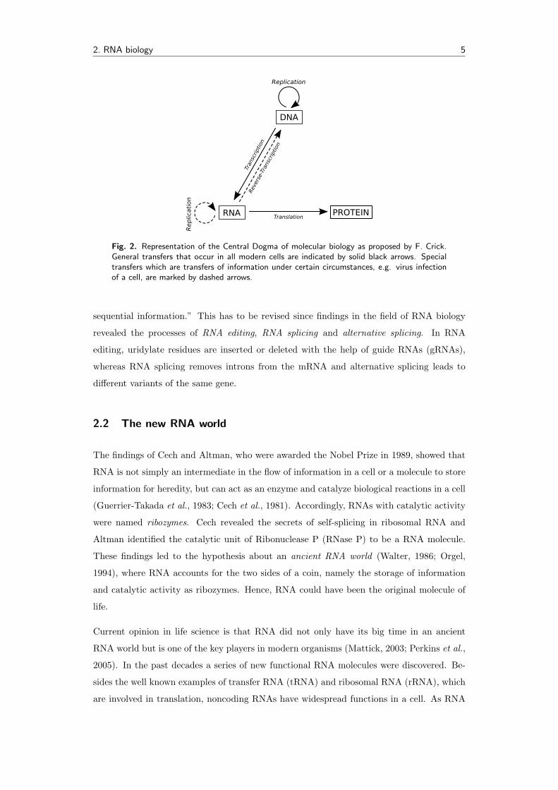
transfers and (ii) the special transfers (see Fig. 2). General transfers refer to the basic
biological processes, replication, transcription, and translation, while special transfers are
only found in cells under certain circumstances, e.g. upon virus infection.
The fact that Crick never stated anything about the amount or control of these processes
(just about the direction of the flow of information) or that RNA has to be ultimately
translated into proteins, guarantees validness up till today. Nevertheless, the Central Dogma
was interpreted the way that RNA was considered as just being an intermediate to promote
translation. This resulted in a protein-centric view of life science for decades. Despite that,
the only point that the dogma meets with criticism is the introductory sentence: “The
central dogma of molecular biology deals with the detailed residue-by-residue transfer of
2. RNA biology 5
Fig. 2. Representation of the Central Dogma of molecular biology as proposed by F. Crick.General transfers that occur in all modern cells are indicated by solid black arrows. Specialtransfers which are transfers of information under certain circumstances, e.g. virus infectionof a cell, are marked by dashed arrows.
sequential information.” This has to be revised since findings in the field of RNA biology
revealed the processes of RNA editing, RNA splicing and alternative splicing. In RNA
editing, uridylate residues are inserted or deleted with the help of guide RNAs (gRNAs),
whereas RNA splicing removes introns from the mRNA and alternative splicing leads to
different variants of the same gene.
2.2 The new RNA world
The findings of Cech and Altman, who were awarded the Nobel Prize in 1989, showed that
RNA is not simply an intermediate in the flow of information in a cell or a molecule to store
information for heredity, but can act as an enzyme and catalyze biological reactions in a cell
(Guerrier-Takada et al., 1983; Cech et al., 1981). Accordingly, RNAs with catalytic activity
were named ribozymes. Cech revealed the secrets of self-splicing in ribosomal RNA and
Altman identified the catalytic unit of Ribonuclease P (RNase P) to be a RNA molecule.
These findings led to the hypothesis about an ancient RNA world (Walter, 1986; Orgel,
1994), where RNA accounts for the two sides of a coin, namely the storage of information
and catalytic activity as ribozymes. Hence, RNA could have been the original molecule of
life.
Current opinion in life science is that RNA did not only have its big time in an ancient
RNA world but is one of the key players in modern organisms (Mattick, 2003; Perkins et al.,
2005). In the past decades a series of new functional RNA molecules were discovered. Be-
sides the well known examples of transfer RNA (tRNA) and ribosomal RNA (rRNA), which
are involved in translation, noncoding RNAs have widespread functions in a cell. As RNA

2. RNA biology 6
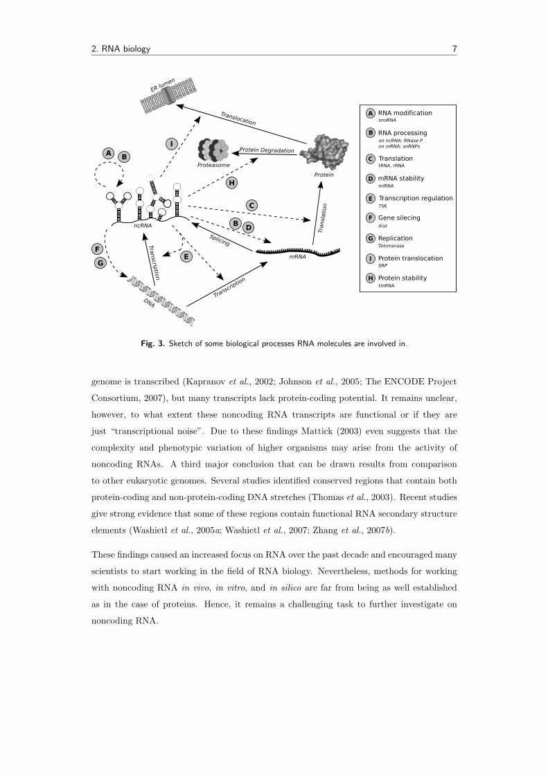
molecules can easily form interactions between themselves, many functional RNAs are in-
volved in biological processes that affect other RNA molecules. RNAse P acts on pre-tRNA
transcripts to yield mature tRNAs, the group of small nuclear RNAs (snRNAs) is involved in
splicing of mRNA (Valadkhan, 2005), and small nucleolar RNAs (snoRNAs) guide chemical
modifications (methylation and pseudouridylation) of ribosomal RNAs (Bachellerie et al.,
2002). As transfer-messenger RNA (tmRNA) has structural and functional properties of
both a tRNA and a mRNA it is able to rescue stalled transcriptional complexes. It is also
involved in protein quality control by adding tags for proteolysis to ribosome-associated
protein-fragments (Dulebohn et al., 2007). In 1993 the first microRNA (miRNA) was iden-
tified in C. elegans (Lee et al., 1993), and until now miRNAs have been discovered in
many eukaryotes. They constitute a key mechanism in post-transcriptional gene regulation,
and some miRNAs have also been reported to be involved in cancer (Zhang et al., 2007a).
Rather than affecting mRNA stability as in the case of miRNAs, 7SK RNA regulates eu-
karyotic gene expression at the level of elongation by sequestering P-TEFb (a cyclin-cdk
complex) into an inactive state (Michels et al., 2004). In mammals dosage compensation
of the two X-chromosomes of female cells is achieved by transitional silencing of one of the
two X-chromosomes mainly mediated by the Xist RNA molecule (Plath et al., 2002). RNA
molecules often constitute essential parts of huge complexes such as the ribosome or the
spliceosome. While in the telomerase complex the RNA molecule serves as a template for
elongating telomeres, the RNA molecule in the signal recognition particle (SRP) is essential
for promoting translocation across the endoplasmic reticulum membrane. A sketch of some
biological processes RNA molecules are involved in is shown in Fig. 3.
The switch away from the picture of a protein dominated world inside a cell to a view where
RNA molecules are also responsible for major, regulatory tasks besides or together with
proteins is mainly due to the discovery of new functional RNA molecules (as outlined above)
and findings that accompany the human genome project (International Human Genome
Sequencing Consortium, 2002; Venter et al., 2001). Of course, the outstanding goal is now
after sequencing is finished to annotate and functionally characterize the human genome.
Surprisingly, recent studies postulated that the human genome contains only around 25,000
to 30,000 protein coding genes (Venter et al., 2001; Pennisi, 2003), which corresponds to a
fraction of about only 1.5% of the total genome. Compared to the nematode C. elegans,
which is said to have approximately 20,000 genes (Hillier et al., 2005), this seems to be a
quite low number of genes. Of course, there are mechanisms like alternative polyadenylation
and alternative splicing which can contribute to enormous increase in protein variants, but
trusting in the results of state-of-the-art gene-prediction software one encounters a paradox.
Namely, that the complexity of an organism is not related to the amount protein coding
genes. Even more surprisingly was the announcement that an enormous fraction of the
2. RNA biology 7
Fig. 3. Sketch of some biological processes RNA molecules are involved in.
genome is transcribed (Kapranov et al., 2002; Johnson et al., 2005; The ENCODE Project
Consortium, 2007), but many transcripts lack protein-coding potential. It remains unclear,
however, to what extent these noncoding RNA transcripts are functional or if they are
just “transcriptional noise”. Due to these findings Mattick (2003) even suggests that the
complexity and phenotypic variation of higher organisms may arise from the activity of
noncoding RNAs. A third major conclusion that can be drawn results from comparison
to other eukaryotic genomes. Several studies identified conserved regions that contain both
protein-coding and non-protein-coding DNA stretches (Thomas et al., 2003). Recent studies
give strong evidence that some of these regions contain functional RNA secondary structure
elements (Washietl et al., 2005a; Washietl et al., 2007; Zhang et al., 2007b).
These findings caused an increased focus on RNA over the past decade and encouraged many
scientists to start working in the field of RNA biology. Nevertheless, methods for working
with noncoding RNA in vivo, in vitro, and in silico are far from being as well established
as in the case of proteins. Hence, it remains a challenging task to further investigate on
noncoding RNA.

3. Computational biology of RNA 8
3 Computational biology of RNA
3.1 RNA Secondary Structure
From a computer scientist’s point of view a RNA sequence is a string S consisting of a series
of characters from a finite alphabet ΣRNA = {A,C,G,U}, where A, C, G, and U represent the
bases adenine, cytosin, guanine, and uracil, respectively. The string S is commonly referred
to as primary sequence. As mentioned above, a single stranded RNA sequence is capable of
folding back to itself and can therefore form extensive secondary structures. A secondary
structure is formally defined as the set of all base-pairs (i, j) the fulfill following criteria:
1. Each base can take part in at most one base-pair.
2. Two base-pairs (i, j) and (k, l) must fulfill either the condition i < j < k < l or the
condition i < k < l < j, i.e. no pseudoknots are allowed.
3. Paired bases must be separated by at least three bases.
3.2 Representations of RNA secondary structures
A very intuitive way of representing RNA secondary structures is the dot-bracket notation,
which is mainly used by the Vienna RNA package. In this representation the secondary
structure is a string over the alphabet ΣSS = {(,),.}. The characters “(“ and “)” corre-
spond to the 5’ base and the 3’ base in the base-pair, respectively, while “.” denotes an
unpaired base. Although this representation is very simple and intuitive in the way that
it follows mathematical rules for parenthesising, there are representations that please the
human eye more and make it easier to visualize various aspects of RNA secondary structures.
Fig. 4. RNA sequence with RNA secondary structure of a typical tRNA in the dot-bracketrepresentation.
3.2.1 RNA secondary structures as planar graphs
As crossing base-pairs (pseudoknots) are not allowed, RNA secondary structures can be
drawn as outer-planar graphs. By definition an outer-planar graph is a planar graph whose
vertices lie on a circle (the sugar-phosphate backbone) and whose edges are inside the disk

3. Computational biology of RNA 9
(Fig. 5a). If this circle is bended up, a representation commonly referred to as dome plot
or arch plot will result (Fig. 5b). The chords in the circle are now turned to become arches.
If those vertexes that form a base-pair are put close together the usual representation of
RNA secondary structures will result (Fig. 5c). All these representations are isomorphic
to each other, i.e. they all encode the same amount of structural information. Graph
representations are often augmented to encode additional information such as base-pairing
probabilities, positional entropy or structural conservation (Fig. 5d and 5e).
Fig. 5. tRNA secondary structure represented as planar graphs. (a) Representation as anouter-planar graph. All vertexes lie on a circle (sugar-phosphate backbone). Pairing bases areindicated by a chord. (b) Representation as dome plot. Base-pairs are marked by arches. (c)Commonly used representation for RNA secondary structures. Note that all these structuresare isomorphic to each other. (d) Secondary structure plot with additional encoding of posi-tional entropy of each nucleotide. (e) Secondary structure plot derived form analysis of a setof aligned tRNA sequences. The color encodes the number of consistent and compensatorymutations supporting that pair. Figures were created with the help of jViz.RNA (Wiese &Glen, 2006) and utilities of the Vienna RNA package.
3.2.2 RNA secondary structures as ordered, rooted trees
While the above described representations as planar graphs are of great value in visual
inspection of RNA secondary structures, the representation as ordered, rooted trees has
proved itself suitable for measuring distances among RNA secondary structures (Shapiro,
1988; Shapiro & Zhang, 1990). The tree representation can be deduced from the dot-bracket
notation, as the brackets clearly imply parent-child relationships. The ordering among the

3. Computational biology of RNA 10
siblings of a node is imposed by the 5’ to 3’ nature of the RNA molecule. To avoid formation
of a forest a virtual root has to be introduced.
The tree representation at full resolution without any loss in information with regard to the
dot-bracket notation can be derived by assigning each unpaired base to a leaf node and each
base-pair to an internal node (Fontana et al., 1993). The resulting tree Tk can be rewritten
to a homeomorphically irreducible tree (HIT) Hk by collapsing all base-pairs in a stem into
a single internal node and adjacent unpaired bases into a single leaf node. Each node is then
assigned a weight reflecting the number of nodes or leafs that were combined.
Shapiro proposed another encoding that retains only the coarse-grained shape of a secondary
structure (Shapiro, 1988). This is useful in the case of comparison of major structural
elements of a RNA molecule but it comes along with a loss of information. A secondary
structure can be decomposed into stems (S), hairpin loops (H), interior loops (I), multi-
loops (M), and external nucleotides (E). While external nucleotides are assigned to a leaf,
unpaired bases in a multi-loop are lost. The weighted coarse-grained approach compensates
the effect of information reduction at least by assigning to each node or leaf the number of
elements that were condensed to this vertex. Representative plots for all tree representations
are given in Fig. 6.
Other forms of abstraction for RNA secondary structures are shapes (Giegerich et al., 2004),
which are discussed in detail in section 4.5.
3.2.3 Mountain representation of RNA secondary structures
A mountain plot is a graph whose x-axis encodes the position of the nucleotide k of a RNA
sequence and the y-axis shows the number of base-pairs (i, j) that enclose the base k in a
way that i < k and k < j (Hogeweg & Hesper, 1984). Generally, this results in a picture
that reminds viewers of a mountain range (see Fig. 7). Peaks correspond to hairpins while
plateaus and valleys correspond to a series of unpaired bases. Plateaus when interrupting
sloped regions represent an interior loop, else a hairpin loop. On the other hand valleys
represent unpaired regions between the branches of a multi-loop, or if their height is zero
an unpaired region spacing structural elements.
This approach can be easily extended to incorporate base-pairing probabilities. A general-
ized version of the mountain representation considering base-pairing probabilities (Huynen
et al., 1996) is outlined below in Eq. 1.

3. Computational biology of RNA 11
Fig. 6. tRNA secondary structure represented as ordered, rooted trees. (a) Full representationof a tRNA secondary structure as proposed by (Fontana et al., 1993). Base-pairs are condensedto a single internal node represented by a blue circle. Unpaired bases are represented as leafnodes indicated by white circles. Compare to Fig. 5c for an equivalent, usual representationof RNA secondary structures. (b) Homeomorphically irreducible tree (HIT) representation.Paired bases in a stem and adjacent unpaired bases are condensed to a single, weightedinternal node and to a single, weighted leaf, respectively. These two representation do notloose any information with regard to the secondary structure in the dot-bracket notation. (c)Coarse-grained tree as proposed by Shapiro (1988). Only the overall architecture of the RNAmolecule is retained. Building blocks of this representation are stem, hairpin loop, internalloop, multi-loop, and external nucleotide nodes. (d) Weighted coarse-grained representation.An extension of the coarse-grained representation by assigning weights to each node to indicatethe number of elements that are covered by the current node.

3. Computational biology of RNA 12
mk =∑
i<k
∑
k<j
pij (1)
This representation gives a weighted average of the Boltzmann ensemble of secondary struc-
tures of a single RNA molecule. Therefore, the value on the y-axis for nucleotide k, gives the
number of base-pairs that are expected to enclose k on average. This visualisation method
with additional encoding of the conservation pattern of a series of aligned RNA molecules
has been successfully applied to the detection of conserved RNA secondary structures in
virus genomes (Hofacker et al., 1998; Hofacker & Stadler, 1999).
Fig. 7. Mountain plot of a typical tRNA secondary structure. In the case of the MFE structurethe y-axis displays the number of base-pairs that enclose a position k. For the average of theensemble it is the number of base-pairs that are expected to enclose k on average.
3.2.4 Dot-plot representation of RNA secondary structures
A dot-plot is a two-dimensional graph, where each base-pair (i, j) of a secondary structure
is marked by a dot or box in the ith row and the jth column. This method of representing a
secondary structure is well suited for visualisation of a weighted set of secondary structures
such as the Boltzmann ensemble of secondary structures. Therefore, the size of the box
or dot is drawn proportionally to the probability pij of the base-pair (i, j). In the layout
that is used by the Vienna RNA package the dot-plot is divided into two triangles. The
upper right triangle corresponds to the base-pairing probability matrix of the ensemble of
structures with box sizes proportional to the probability of the corresponding base-pair. The
lower left triangle visualizes the MFE structure with equally sized boxes (see Fig. 8).

3. Computational biology of RNA 13
Fig. 8. Dot-plot of a typical tRNA secondary structure. The upper right triangle of theplot visualizes the base-pairing probability matrix of the ensemble of structures with boxsizes proportional to the probability of the corresponding base-pair. The lower left trianglerepresents the MFE structure with equally sized boxes.

3. Computational biology of RNA 14
3.3 RNA folding algorithms
3.3.1 Loop-based energy model
RNA secondary structures can be uniquely decomposed into loops. A position k is called
immediately interior of the base-pair (i, j) if i < k < j and there is no other base-pair (p, q)
such that i < p < k < q < j. Any loop is therefore uniquely determined by its closing
pair (i, j) and we can write Li,j to denote the loop L closed by the base-pair (i, j). Those
nucleotides that are not enclosed by a base-pair are gathered in the exterior loop L0. Hence,
a secondary structure S can be described as the union of all loops Li,j and the exterior loop
L0.
S = L0
⋃ ⋃
(i,j)∈S
Li,j
(2)
A loop can be formally characterized by its length, i.e. the number of unpaired bases and
by its degree k. The degree k of a loop is defined by the number of base-pairs delimiting
the loop. Loops of degree 1 are called hairpin loops, interior loops have a degree of 2, and
multi-loops have more than 2 delimiting base-pairs. Bulge loops are special cases of interior
loops, where only one side has unpaired bases and stacked pairs are referred to as interior
loops with length zero (see Fig. 9).
The k-loop decomposition forms the basis of the standard energy model used by the Vienna
RNA package, as Eq. 2 can be directly converted to an energy function. Assuming indepen-
dence of the loops and that the total energy E(S) of a secondary structure S is the sum of
the energy contributions of the single loops e(L) allows efficient computation of the minimal
free energy (MFE) structure of a RNA molecule by dynamic programming.
E(S) = e(L0) +∑
(i,j)∈S
e(Li,j) (3)
Current RNA secondary structure models consider free energy differences between unfolded
and folded states in aqueous solution. Energy parameters for those models are derived
empirically by RNA oligomer unfolding experiments. An extensive collection of energy
parameters is maintained by the group of David Turner (Xia et al., 1998; Mathews et al.,
1999b). Major energy contributions are base stackings, hydrogen bonds, and loop entropies.
Loop energies depend on the loop degree k and the loop length. While for stacked base-pairs
and small hairpin loops one can fall back on tabulated parameters, energies for other loops

3. Computational biology of RNA 15
Fig. 9. Loop decomposition of a secondary structure. Loops are characterized by its length,i.e. the number of unpaired bases and by its degree k, which is simply the number of base-pairsdelimiting the loop. Hairpin loops are of degree 1, and multi-loops have a degree greater than2. Loops of degree 2 can be subdivided into interior loops (unpaired bases on both sides),bulge loops (unpaired bases on only one side), and stacked base-pairs with a loop size of zero.
are approximated by simplified models derived from the field of polymer theory.
3.3.2 Folding of single sequences
First attempts at RNA secondary structure prediction aimed at finding a maximum matching
on a sequence, i.e. maximizing the number of base-pairs. Nussinov et al. (1978) proposed an
algorithm based on the idea of dynamic programming guided by previous work by Waterman
(1978) and Waterman & Smith (1978). Although this non-thermodynamic model is too
simple for accurate secondary structure prediction it is a stepping-stone for later algorithms
as they all make use of this general principle. The basic concept of dynamic programming
is to use the optimal solutions of subproblems to find an optimal solution to the overall
problem, formally known as the Bellman principle of optimality (Bellman, 1957).
Let us consider a RNA sequence x with a length of n nucleotides. xi denotes the ith
nucleotide in sequence x. The set of valid base-pairs Π consists of Watson-Crick base-
pairs and the GU-wobble base-pair. For ease of computation no restrictions are made on
a minimal spacing for the closing base-pair of hairpin loops. The only requirement we
have to postulate is the exclusion of pseudoknots as this would conflict with our dynamic
programming approach. A subsequence will be denoted by x[i..j], the maximum number

3. Computational biology of RNA 16
of base-pairs on that subsequence is given by Mi,j . The basic idea is that a structure on
a subsequence x[i..j] can only form in two distinct ways. Assuming that we have already
calculated the maximum matching on the interval x[i..j−1] the newly added base xj is either
unpaired followed by an arbitrary structure on x[i..j − 1], or xj interacts with a nucleotide
xk on the interval xi ≤ xk ≤ xj−1.
Fig. 10. Decomposition of the subsequence x[i..j] used in the maximum matching algorithm.Either xj is unpaired followed by an arbitrary structure on x[i..j − 1], or base xj interactswith a nucleotide xk on the interval xi ≤ xk ≤ xj−1.
If xj can form a valid base-pair with position xk, then the subsequence x[i..j] will be split
into two subsegments x[i..k − 1] and x[k + 1..j − 1], for which the maximum matching has
already been computed. The maximum matching on subsequence x[i..j] is hence given by
the recursion outlined in Eq. 4.
Mi,j = max
Mi,j−1
maxi≤k≤j−1(k,j)∈Π
(Mi,k−1 + Mk+1,j−1 + 1)(4)
While this recursion gives the maximal number of base-pairs m sequence x can have, it does
not immediately tell the secondary structure with m base-pairs. The list of base-pairs that
constitute a secondary structure with m base-pairs has to be derived via backtracing. That
is simply inverting the algorithm using the calculated values from the forward recursion to
reconstruct the optimal path (set of base-pairs) that gave rise to the maximum matching of
the overall sequence.
The effort of the naıve approach of a full enumeration of all possible structures on a RNA
sequence is exponentially related to the length of the sequence. With the help of dynamic
programming the exponential complexity can be reduced to O(n3) in CPU power and O(n2)
in memory requirements.
First improvements of the maximum matching method considered assigning binding energies
to base-pairs. Eq. 4 can be used straightforward to set up a simple thermodynamic model
using an energy parameter βij describing the stability of the base-pair (i, j). According to
the prerequisites postulated before Ei,j denotes the minimum energy on the interval x[i..j].

3. Computational biology of RNA 17
Ei,j = min
Ei,j−1
mini≤k≤j−1(k,j)∈Π
(Ei,k−1 + Ek+1,j−1 + βkj)(5)
Unfortunately, this simple modification to Eq. 4 does not create viable secondary structures
one would expect in nature, and thus state-of-the-art implementations for minimum free
energy calculations of RNA secondary structures stick to the loop dependent energy model
discussed in section 3.3.1. Although the overall computational complexity is still O(n3),
recursions and backtracing become more sophisticated.
At room temperature the folding of a RNA sequence is not restricted to a single structure.
McCaskill (1990) proposed an elegant way of computing the partition function Z over all
structures of a RNA sequence by dynamic programming.
Z =∑
S
e−ESRT (6)
The framework of dynamic programming allows to efficiently compute the equilibrium prob-
ability of a structure, and in addition the frequency of a base-pair occurring in the Boltzmann
weighted ensemble of structures, which can be easily visualized in the form of a dot-plot.
3.3.3 Folding of multiple sequence alignments
Gutell et al. (2002) impressively demonstrated the power of comparative sequence analysis
on a large set of 7,000 rRNAs. In their study they were able to predict almost all of
the standard secondary structure base-pairings of the 16S rRNA and 23S rRNA crystal
structures without referring to a thermodynamical model for energy minimization. Their
method is solely based on exploiting covariation of a set of related sequences by utilizing
the fact that functional RNA molecules are under evolutionary pressure to preserve their
secondary structure.
The aim of each RNA secondary structure prediction algorithm is, of course, to get as close to
the native, biological active conformation as possible. Using a thermodynamic model alone
often yields unsatisfying results, e.g. in its current version the Rfam database holds more
than 84,000 (redundant) tRNA sequences but only a minority of them will have the typical
cloverleaf structure as the predicted minimum free energy structure. Based on the idea of
comparative sequence analysis Hofacker et al. (2002) proposed the RNAalifold algorithm
that extends the standard energy minimization algorithm by phylogenetic information in
form of sequence covariation. RNAalifold allows efficient computation of the consensus

3. Computational biology of RNA 18
structure of a set of aligned RNA sequences.
A measure to score sequence variation often used in the context of comparative RNA se-
quence analysis is the mutual information (MI) outlined in Eq. 7, where fi,j(a, b) is the
frequency of finding a in the ith column and b and the jth column, and fi(a) and fj(b) is
the frequency of a in column i and b in column j, respectively.
MIi,j =∑
ab
fi,j(a, b) log2
fi,j(a, b)fi(a)fj(b)
(7)
As the mutual information quantifies the information in a pair of columns it is clear that
total conservation will yield MIi,j = 0. But this also happens if only one column varies as it
in the case of consistent mutations such as G • C to G • U. By neglecting cases of consistent
mutations the signal of mutual information is, in general, too weak on spare data sets.
The RNAalifold algorithm uses a covariance measure Ci,j that is capable of distinguishing
between conserved pairs, pairs with consistent mutations, and pairs with compensatory
mutations. It is guided by the assumption that the more mutations that preserve a certain
base-pair, the more evidence is given that the base-pair is correct.
Ci,j =∑
ab,a′b′fi,j(a, b)D(a,b),(a′,b′)fi,j(a′, b′) (8)
The 16 × 16 matrix D has entries D(a,b),(a′,b′) corresponding to the Hamming distance if
both pairs (a, b) and (a′, b′) are in the set of valid base-pairs, and D(a,b),(a′,b′) = 0 otherwise.
A formulation of covariance this way ensures that consistent and compensatory mutations
are rewarded, but it does not penalize inconsistent pairs. Inconsistent pairs are all non-
Watson-Crick and non-GU pairs, and combinations of a nucleotide with a gap character.
The measure qi,j simply counts the number of inconsistent pairs, which can be subsequently
used with the covariance Ci,j for a combined score Bi,j , where φ1 is a scaling factor.
Bi,j = Ci,j − φ1qi,j (9)
A comparison of Bi,j to a threshold value B∗ is used to decide whether two columns can
pair on the alignment level, or not. It is now straightforward to extend the simple energy
model outlined in Eq. 5 to the purpose of predicting a consensus structure of a set of aligned
RNA sequences by modifying the energy parameter βij , as shown in Eq. 10.

3. Computational biology of RNA 19
βAij =1N
N∑
k
ε(aki , ak
j )− φ2Bi,j (10)
ε(aki , ak
j ) is the energy contribution of the base-pair (i, j) in sequence k, and φ2 a scaling
factor. The updated energy model uses now βAij as the average of the pairing energy combined
with covariation score B. Lindgreen et al. showed that the RNAalifold covariance measure
is more discriminative than the mutual information and is a good choice due to its simplicity.
With some modifications this model can be applied to the loop-based energy model as well.
The consensus energy is then computed by averaging over the loop-based energies plus
covariance contributions of all sequences.
3.4 The race for computational ncRNA detection
The emerging interest in noncoding RNAs has also led the scientific community to focus on
the development of computational tools that are capable of detecting novel ncRNAs. But
finding ncRNAs in genomic sequences has proved to be difficult for several reasons. Unlike
for proteins it is very difficult to define general start and end points, ncRNAs vary in size and
have few common statistical features. Nevertheless, there are many efforts to develop tools
that try to exploit the sparse common features of ncRNAs. First attempts mainly focused
on predicting novel RNA molecules of a certain family, that has a well characterized family
folding motif (Lowe & Eddy, 1997; Lai et al., 2003). An extensive overview of methods
is given in reference (Athanasius F Bompfunewerer Consortium et al., 2007), that lists for
example at least eleven tools for the purpose of predicting miRNAs.
As mentioned before, the structure of a RNA molecule is often more biologically relevant
than its sequence. Hence, one might think that functional noncoding RNAs should have,
in general, a more thermodynamically stable structure than a random sequence with the
same base composition. It would be straightforward to use this feature for an all purpose
ncRNA detection application. Thermodynamic stability can be expressed in terms of a
z-score, which involves comparison of the minimum free energy of the native sequence to
a large population of randomized alignments with the same properties. Unfortunately, this
method will have a very high false positive rate when applied in a genomic screen (Rivas &
Eddy, 2000). Washietl & Hofacker (2004) proposed a method, AlifoldZ, that is based on
the idea of the z-score but takes structural conservation over a set of aligned RNA sequences
into account. Up to now, most bioinformatic tools that allow general prediction of ncRNAs
utilize the power of comparative analysis between sequences that are related on nucleotide
level in different ways (Rivas & Eddy, 2001; di Bernardo et al., 2003; Coventry et al., 2004;

3. Computational biology of RNA 20
Washietl et al., 2005b; Pedersen et al., 2006). The approach of doing de novo detection of
evolutionarily conserved structural RNA elements on a set of related sequences rather than
on single sequences seems to be the most reasonable one at the moment and gains ground
as more sequence data is becoming available through various sequencing projects.
All current methods try to evaluate the effect of mutations on the nucleotide level in relation
to secondary structure by different methods. In the case of QRNA (Rivas & Eddy, 2001) and
EvoFold (Pedersen et al., 2006) stochastic context free grammars with different evolutionary
models for coding sequences and sequences with an RNA secondary structure constraint are
used. ddBRNA (di Bernardo et al., 2003) counts compensatory mutations in all possible
stem loops and MSARI (Coventry et al., 2004) uses a statistical test over significant base-
pairs. RNAz (Washietl et al., 2005b) uses a combination of two features, namely the average
of the z-scores of the single sequences in an alignment and a measure for the structural
conservation called structure conservation index (SCI). The SCI is defined as the ratio of
the energy derived by constraint folding of all single sequence into a common secondary
structure using the RNAalifold algorithm and the average over the energies of the single
sequences folded individually. Although secondary structure conservation is only measured
indirectly in terms of energies, this approach turned out to be relatively accurate and RNAz
has been applied successfully to a wide range of genomic ncRNA predictions (Missal et al.,
2005; Missal et al., 2006; Washietl et al., 2005a; Washietl et al., 2007).
3.5 The RNAz algorithm
Using RNA secondary structure prediction tools such as RNAfold (Hofacker et al., 1994)
or mfold (Mathews et al., 1999a) it is easy to calculate the minimum free energy of a
given RNA sequence. As the MFE depends on length and base composition one usually
calculates for use of the MFE as a measure of thermodynamic stability a z-score. That
can be done by comparing the MFE m of a given RNA sequence to the MFEs of a large
number of random sequences of the same length and base composition. A z-score is then
calculated as z = (m-µ)/σ, where µ and σ are the mean and standard deviations of the
MFEs of the random samples, respectively. Negative z-scores indicate that a sequence is
more stable than expected by chance. To speed up computation RNAz does not rely on
explicit (mononucleotide) shuffling but uses a support vector machine (SVM) for regression
to determine the mean energy and standard deviation for given nucleotide frequencies and
length.
In general, functional RNAs are known to be thermodynamically more stable (Clote et al.,
2005). On the other hand Rivas & Eddy (2000) showed that using this feature alone for

3. Computational biology of RNA 21
noncoding RNA detection in whole genome screens is not accurate enough as it would
result in a high number of false positives. To address this problem RNAz uses a combined
approach. Besides thermodynamic stability structural conservation is taken into account.
The structure conservation index (SCI) will be discussed in more detail in section 4.1, hence
only the main principle will be outlined here.
The RNAalifold algorithm is used to compute the consensus structure and hence consensus
energy of a multiple sequence alignment of RNA sequences. Rather than to evaluate the
quality of the consensus energy against a randomized population (Washietl & Hofacker, 2004)
the consensus energy is set in relation to the mean of the unconstrained folding energies of
the single sequences. The consensus energy of sequences that share indeed a common fold
will be close to or due to bonus energies rewarded for compensatory mutations even lower
than the mean energy of the single sequences, resulting in a SCI close to or even higher than
1. On the other, for sequences that do not have a common fold RNAalifold is not likely to
find a “good” consensus structure, and hence the SCI will be close to 0.
As RNAz makes use of a SVM for final classification, the main concept of support vector
machines will shortly be describe here. Consider a classification problem that is linearly
separable (see Fig. 11). Then the optimum separation hyperplane is the hyperplane H with
maximum distance to each of the two hyperplanes H1 and H2.
Fig. 11. Linearly separable classification problem. The optimal classifier is the hyperplane Hwith maximum distance to each of the two hyperplanes H1 and H2.
SVMs are also able to handle nonlinearly separable classification problems. In this case the
feature space is expanded via a kernel function to a higher-dimensional feature space. The
maximum margin hyperplane in the higher-dimensional space gives a nonlinear decision
boundary in the lower-dimensional, original feature space. This concept is schematically
shown in Fig. 12.
For final classification RNAz uses a four dimensional feature vector composed of the z-score,
the SCI, and two additional features that are mainly required for “interpretation” of the

3. Computational biology of RNA 22
SCI, namely the number of sequences, and the average pairwise identity. With decreasing
average pairwise identity the SCI is also expected to have lower values. The more sequences
are contained in an alignment the more evidence is given that predicted consensus structure,
and with that the consensus energy and the SCI, are correct. However, one has to keep in
mind that the more features are added to SVM, the bigger the feature space gets and the
more training instances are needed to sample the feature space. This thesis also investigates
the normalized Shannon entropy as another sequence and alignment variation measure,
which may help to reduce the features of the RNAz SVM.
Fig. 12. A nonlinearly separable classification problem is transform via a kernel function toa higher-dimensional feature space. The maximum margin hyperplane then gives a nonlineardecision boundary in the lower-dimensional, original feature space.
In the following we will investigate different methods that can be consulted to assess struc-
tural conservation, to finally improve the performance of RNAz. The SCI does well, but
other methods may perform better in special ranges or the SCI in combination with other
methods may yield an even better classifier.

4. Strategies for measuring evolutionary conservation of RNA secondary structures 23
4 Strategies for measuring evolutionary conservation of RNA
secondary structures
There is consensus in the scientific community that the information a single sequences carries
is, in general, not enough for accurate distinction of functional RNAs from background.
A common strategy is to exploit the information contained in a set of related sequences.
As functional RNAs are subjected to evolutionary pressure, mutations that preserve the
functional structure will accumulate over mutations that change the structure drastically.
Hence, it is important to find strategies that are able to efficiently measure the degree of
structural conservation to help to identify in combination with other statistical properties
such as thermodynamic stability conserved, functional RNAs.
When comparing RNA secondary structures the result can be quantified in two ways, either
as a distance or as a similarity measure. A similarity measure reflects the strength of the
relationship between two objects in a metric space. The higher the similarity the closer two
objects are in this space. The notion of distance used in this work satisfies the mathematical
axioms of a metric. A distance therefore indicates how far two points are from one another
in a metric space. Hence, the distance of two equal objects is always zero. In contrast, a
similarity measure will yield an arbitrary positive number. Accordingly, a small distance is
related to a high similarity.
This chapter will focus on various distance and similarity measures for RNA secondary struc-
ture comparison that can be consulted to assess the conservation of a set of RNA sequences.
As many of these strategies act solely on secondary structures, the way of generation, either
by comparative analysis, thermodynamic energy minimization or context free grammars,
will not influence the underlying algorithms for structure comparison.
Some methods can act solely on structures of the same length. Assuming a set of related
sequences it is likely that insertions or deletions may be observed in some sequences, so
that sequences differ in length. One strategy to overcome this drawback is to fold the
sequences without gap characters and then use the alignment of the sequences as guidance to
reconstruct the original positions that are said to match. In the case of secondary structures
in dot-bracket notation this simply means inserting “.” in the secondary structure for each
corresponding gap character in the sequence. When applied to base-pairing probabilities
one has to adjust the consecutive numbers of the nucleotides that form the base-pair.
As many methods are only suited for pairwise structure comparison, we will use the aver-
age pairwise distance or the average pairwise similarity to asses structural conservation of

4. Strategies for measuring evolutionary conservation of RNA secondary structures 24
sequences in a multiple sequence alignment. For those strategies that allow to make use of a
consensus structure, the average distance of the sequences in the alignment to the consensus
structure will be considered as well.
4.1 Minimum free energy based methods
The idea to evaluate the conservation of a set of RNA sequences by the minimum free energy
rather than by the minimum free energy structures seems to be unusual at first glance. But
the principle soon becomes clear when considering the RNAalifold algorithm for a set of
aligned sequences that share a common secondary structure. Assuming reasonable quality
of the alignment with regard to secondary structure, running RNAalifold on this alignment
will, in general, result in a relatively “good” energy compared to an alignment with the
same properties (the same length, the same number of sequences, the same gap pattern and
the same degree of local conservation) but without a common secondary structure. This
seems to be a reasonable strategy but the challenge is how to judge “good”. A possible
way of doing that is by means of a z-score, which is implemented in the program AlifoldZ
(Washietl & Hofacker, 2004). For the alignment to be evaluated, the consensus energy is
computed and compared to the mean energy of a randomized alignment population with
the same properties. This approach is computationally relatively expensive as it requires
explicit shuffling and evaluation of the random samples. Another possible approach is to set
the consensus energy in relation to the mean of the energies derived by folding each sequence
individually. This leads directly to the definition of the structure conservation index (SCI)
as proposed by Washietl et al. (2005b) .
SCI =Econsensus
〈Esingle〉 (11)
If all the sequences in an alignment are able to fold into a common secondary structure,
the consensus energy will be close to the average of the mean of the energies of the single
sequences, yielding a SCI close to 1. With bonus energies that are assigned for compensatory
and/or consistent mutations by RNAalifold, a SCI even higher than 1 is possible. Although
structural conservation is only measured indirectly at energy levels the SCI has asserted itself
as a powerful strategy for identifying evolutionary conserved RNA secondary structures.
Gardner et al. (2005) even use the SCI to evaluate the performance of multiple sequence
alignment programs upon structural RNAs.
Guided by these findings we are free to postulate other methods for assessing RNA structure
conservation in terms of folding energies. The tool RNAeval from the Vienna RNA package

4. Strategies for measuring evolutionary conservation of RNA secondary structures 25
(Hofacker et al., 1994) can be used to evaluate the free energy of an RNA molecule in a given
secondary structure. Based on the assumption that a set of evolutionary related sequences
is expected to share more or less the same structure one can set up all pairwise combinations
and evaluate the energy of a sequence under the constraint of being forced to fold into the
structure of another sequence. Again as mentioned for the SCI above, this energy should
be close to the energy of the sequence folded individually. Eq. 12 outlines this method for
an alignment A, where E(x) is the minimum free energy of sequence x, Sy is the structure
of a sequence y and E(x|Sy) is the energy derived by RNAeval by evaluating the energy of
sequence x under the constraint of folding into the structure of sequence y. As this method
can only be applied on sequences of equal length one has to use sequences including gap
characters for structure prediction and evaluation.
SCIRNAeval,pairwise(A) =
∑x,y∈A
x6=y
E(x|Sy)
(|A| − 1)∑
x∈AE(x)
(12)
Using RNAeval one can also set up a SCI-like variant by evaluating the energy of the se-
quences in the alignment in the consensus structure Sconsensus derived by RNAalifold.
This way the bonus energies that are rewarded by RNAalifold for consistent and/or com-
pensatory mutations will not be considered. This model could be used to study the effect of
the bonus energy on the discrimination power but as RNAeval and RNAalifold use differ-
ent strategies for handling gaps in their current implementations, it would give misleading
results. As bonus energies are used throughout all recursions for energy minimization in
the RNAalifold algorithm and not just simply added at the end, it is advisable to study
the effect of bonus energies by explicitly disabling the use of bonus energies in RNAalifold.
This will not only effect the minimum free energies but may also lead to different secondary
structures.
4.2 Tree editing methods
As shown in section 3.2.2, RNA secondary structures can be represented as ordered, rooted
trees. Besides visual examination of secondary structures, tree representations can be used to
calculate distances between RNA secondary structures. Tree editing induces a metric in the
space of trees and therefore a metric in the space of RNA secondary structures. Tree editing
uses three elementary editing operations: substitution, insertion, and deletion. Substitution
(x → y) is defined as replacing a vertex label x by another vertex label y. Therefore it is
often called simply relabeling. Deleting a vertex x (x → ∅) is accompanied by assigning the
children of node x to become children of the parent node of vertex x. The insertion of a

4. Strategies for measuring evolutionary conservation of RNA secondary structures 26
vertex x (∅ → x) is complementary to the deletion. A new vertex x is inserted in a tree as
the child of a vertex z thereby making the children of z now children of the newly inserted
vertex x. Tree editing operations are illustrated in Fig. 13.
Fig. 13. Elementary operations in tree editing. Tree T1 can be transformed into tree T2
by substitution, and vice versa. By deletion of the vertex with the label X tree T2 can betransformed into tree T3. The opposite way round T2 results by inserting the vertex with labelX from T3.
A cost is assigned to each of this editing operations. Intuitively, a deletion of a single
leaf in the representation at full resolution is 1, while the deletion of an internal node
that corresponds to a base-pair is of cost 2. In addition weights can be assigned to nodes
representing the number of structural elements that were condensed to this single node, e.g.
in the case of the HIT representation or the weighted coarse-grained representation. The
cost function of an editing operation can then be modified to take weights into account.
A sequence of operations that transforms a tree Ti into a tree Tj is called an edit script. The
cost of an edit script is the sum of the cost of the edit operations in the script. The distance
between two trees d(Ti, Tj) is then defined as the cost of the edit script with minimal
cost. As tree editing operations preserve the relative traversal order of the tree nodes,
tree editing can be regarded as a generalization of the sequence alignment problem. This
problem is addressed by RNAforester (Hochsmann et al., 2004), but will not be considered
in this thesis. For trees that consist solely of leaves tree editing becomes standard sequence
alignment.
In this work we will focus on two different implementations of tree editing. RNAdistance
(Hofacker et al., 1994) a tool from the Vienna RNA package implements a tree editing
algorithm initially proposed by Shapiro (1988) and acts on the full representation, HIT
representation (Fontana et al., 1993), coarse-grained and weighted coarse-grained represen-
tation (Shapiro, 1988). Properties of these representations are discussed in detail in section
3.2.2. For the coarse-grained and weighted coarse-grained representation RNAdistance pro-
vides two different scoring models based on the costs initially proposed by Shapiro (1988)
and redefined costs used in the Vienna RNA package.
Allali & Sagot (2005a) postulated some shortcomings of the classic tree editing operations
and introduced novel editing operations called node-fusion and edge-fusion. By definition,

4. Strategies for measuring evolutionary conservation of RNA secondary structures 27
Fig. 14. Output of a comparison of two RNA secondary structures using the MiGaL algorithm.Color code represents the structural elements, which are subsequently derived by addition ofmore structural detail. The color is then used as a additional feature in the comparisonalgorithm. Level 0 is the network of multi-loops and is hence the most coarse-grained rep-resentation (nodes in the corresponding tree correspond to multi-loops). Level 1 encodesthe architecture defined by stems (internal nodes correspond to multi-loops, leaves representhairpin-loops, and edges represent stems). Level 2 encodes secondary structure elements de-fined by loops (multi-loop, hairpin loop, interior and bulge loop). Level 3 is a tree at fullresolution including nucleotides as labels.

4. Strategies for measuring evolutionary conservation of RNA secondary structures 28
the standard tree editing algorithm can only associate one element in the first tree with
one element in the second tree. Consider the example of having a helical region in the first
tree and the same helical region interspersed by a small internal loop in the second tree.
Any representation that uses abstraction of individual base-pairs and unpaired bases will
show in the case of the second tree more than one structural element. It seems reasonably
to associate the helix in the first tree to the two helices in the second tree. Thus, the edit
operation edge-fusion is introduced to handle these cases. A very similar problem arises
when considering a small helix between two structural elements present in one tree but not
in the other one. Hence, it would be convenient to associate nodes of the small helix of the
first tree to two or more nodes in the second tree. This is managed by the new edit operation
node-fusion. As Allali makes use of the RNA sequence in his tree model as well, i.e. the
label of each node in the tree model is assigned the corresponding nucleotide, a new problem
arises: nodes in the first tree will be mapped to nodes with identical labels in the second tree
to minimize the total cost of editing operations although these nodes may belong to different
structural elements. To tackle this “scattering effect” a new data structure called multiple
graph layers (MiGaL) is introduced (Allali & Sagot, 2005b). It is capable to encode data
at different levels of detail. Each level is a graph representing a refinement of the preceding
level. Applied to the field of RNA comparison, the bottom layer consists of the secondary
structure at nucleotide level, while the top layer encodes the network of multi-loops of an
RNA secondary structure. The algorithm works top down, i.e. starting the comparison at
the most coarse grained level. The result of a comparison is transmitted to the next layer
by coloring vertexes and edges. Then tree editing operations are only applied to structural
elements of the same color. A sample output is shown in Fig. 14.
In this study a normalized tree editing distance is used for all methods. It is defined as the
ratio of the distance between two secondary structures Sx and Sy to the sum of the costs of
deleting either of the two secondary structures. Deleting a secondary structure is defined as
the cost of comparing a secondary structure S to an empty structure denoted as •.
Dnorm(Sx, Sy) =d(Sx, Sy)
d(Sx, •) + d(•, Sy)(13)
4.3 Methods based on base-pair distances
The base-pair distance between two structures SA and SB is defined as the number of base-
pairs not shared by the two structures. This can be easily described in terms of set theory
as the symmetric set difference:

4. Strategies for measuring evolutionary conservation of RNA secondary structures 29
dBP (SA, SB) = |SA \ SB | ∪ |SB \ SA| = |SA ∪ SB | − |SA ∩ SB | (14)
= |SA|+ |SB | − 2|SA ∩ SB | =∑
i<j
(δAij + δB
ij − 2δAijδ
Bij)
δSij =
1 (i, j) ∈ S
0 else
(15)
dBP itself is not a suitable measure for comparison as long it is not set in relation to the union
of the base-pairs in SA and SB . Clearly, it is a difference if dBP is five for two sequences that
have in total ten base-pairs or in total fifty base-pairs. The normalized base-pair distance
scaled to the interval [0, 1] between two structures is given by:
DBP (SA, SB) =|SA ∪ SB | − |SA ∩ SB |
|SA ∪ SB | =
∑i<j
(δAij + δB
ij − 2δAijδ
Bij)
∑i<j
(δAij + δB
ij − δAijδ
Bij)
(16)
The base-pair distance is sensitive to the exact position of the base-pairs. This effect
can be drastically demonstrated in the case of shifted structures. Assuming SA to be
.......(((...))).. and SB to be ........(((...))). results in a maximal normalized
base-pair distance of 1, as these two structures do not have a single base-pair in common.
Hence, the quality of the alignment with regard to secondary structure will strongly influence
the results.
RNA molecules are commonly known to exist in an ensemble of structures, which can be
modeled by an energy weighted Boltzmann distribution. The probability of a single structure
S in the ensemble of structures S is given by equation Eq. 17, where the partition function
Z is outlined in Eq. 18. R is the molar gas constant and T is the absolute temperature.
The base-pair probability pij of the bases i and j is then given by Eq. 19, where δij is 1 if
the base-pair (i, j) is formed in structure S and 0 otherwise.
P (S) =e−ES/RT
Z(17)
Z =∑
S∈S
e−ES
RT(18)

4. Strategies for measuring evolutionary conservation of RNA secondary structures 30
pij =∑
S∈SP (S)δij (19)
Using these assumptions the equation of the base-pair distance can be remodeled to calculate
the average base-pair distance 〈dBP (SA,SB)〉 between all structures of the two ensembles
SA and SB .
〈dBP (SA,SB)〉 =∑
SA∈SA
∑
SB∈SB
[P (SA)P (SB)
∑
i<j
(δAij + δB
ij − δAijδ
Bij)
](20)
=∑
i<j
[ ∑
SA∈SA
P (SA)δAij
∑
SB∈SB
P (SB)
+∑
SB∈SB
P (SB)δBij
∑
SA∈SA
P (SA)
−2∑
SA∈SA
P (SA)δAij
∑
SB∈SB
P (SB)δBij
]
=∑
i<j
[pA
ij + pBij − 2pA
ijpBij
]
This equals the naıve approach of multiplying the probability of the base-pair (i, j) in the
ensemble SA with the probability of not expecting the base-pair (i, j) in the ensemble SB and
vice versa. Taking a closer look at Eq. 21, one will soon realize that 〈dBP (SA,SA)〉 is not
zero as this is the average distance between the structures in the ensemble1. Thus, to ensure
identity, symmetry and the triangle inequality the ensemble distance Densemble(SA,SB)
between two ensembles SA and SB is defined as follows:
Densemble(SA, SB) = 〈dBP (SA,SB)〉 − 12(〈dBP (SA,SA)〉+ 〈dBP (SB , SB)〉) (21)
=∑
i<j
[pA
ij + pBij − 2pA
ijpBij
]− 12
∑
i<j
[2pA
ij − 2pAij
2]− 1
2
∑
i<j
[2pB
ij − 2pBij
2]
=∑
i<j
[pA
ij + pBij − 2pA
ijpBij − pA
ij + pAij
2 − pBij + pB
ij
2]
=∑
i<j
[pA
ij
2+ pB
ij
2 − 2pAijp
Bij
]=
∑
i<j
(pA
ij − pBij
)2
4.4 Methods based on the mountain metric
The mountain metric is based on the mountain representation of RNA secondary structures
and follows the idea that the distance between two structures SA and SB can be expressed
as the difference of the two mountain graphs. For this purpose a lp-norm can be defined
1RNAfold in its current version outputs this measure as the ensemble diversity, sometimes also referred toas well-definedness. Freyhult et al. (2005) investigate the potential of the ensemble diversity to discriminatebetween ncRNAs and random sequences.

4. Strategies for measuring evolutionary conservation of RNA secondary structures 31
that induces a metric dpM on two secondary structures SA and SB as the difference of the
two mountain functions m(SA) and m(SB) (Moulton et al., 2000):
dpM (SA, SB) :=‖ m(SA)−m(SB) ‖:= (
n∑
i=1
|mi(SA)−mi(SB)|p) 1p (22)
For ease of computation the height m at position k can be defined as the number of “(”
brackets minus the number of “)” brackets but in this work we will stick to the definition
initially proposed in section 3.2.3 where the height m at position k is the number of base-
pairs that enclose k as this will assure consistency when using base-pairing probabilities.
The metric dpM using the height m defined this way will weight base-pairs differently. This
can be shown by a simple example, where SA = ..(...).. and SB =(.......) are
compared to the open chain given by S0 = ........., which yields d1M (SA, S0) = 3 and
d1M (SB , S0) = 7. This effect can be overcome by scaling the height mk as shown in Eq. 23
for the MFE structure and Eq. 24 for the average of the ensemble of secondary structures,
respectively. In the case of applying dpM on the MFE structure a single base-pair in any
position will therefore have a dpM of one, while for the average of the ensemble dp
M will equal
pij .
mk =∑
i<k
∑
k<j
1j − i− 1
(23)
mk =∑
i<k
∑
k<j
pij
j − i− 1(24)
As dpM is expected to grow with the length of sequences, we are in the need of defining
a normalized distance measure to be able to compare alignments of different length. The
maximal distance dpmax of a secondary structure x on a sequence of length n compared to
the open chain of length n is achieved if x is a stem of maximal height (b(n− 3)/2c) with a
hairpin loop of three unpaired bases. The normalized mountain metric DpM is then defined
as the relation of the distance dpM (SA, SB) of two secondary structures with length n to the
maximal distance dpmax at length n. In this study d2
M generally referred to as the root mean
squared (RMS) distance was used. Although the mountain metric has been discussed in
literature quite often, there are only a few cases of successful application (Edvardsson et al.,
2003; Moulton et al., 2000).

4. Strategies for measuring evolutionary conservation of RNA secondary structures 32
4.5 RNAshapes
As outlined before, RNA molecules exist in vivo rather as an ensemble of secondary struc-
tures than as one single secondary structure. Two related RNA sequences might have very
different MFE structures, but at the same time might share the same structure in a small
energy range just above the MFE. There are various programs that allow prediction of sub-
optimal structures (Wuchty et al., 1999; Zuker, 1989). This procedure is computationally
exhaustive as the folding space of a RNA molecule is substantially smaller than the sequence
space but still exponentially related to the length of the RNA molecule (Zuker & Sankoff,
1984). Besides this scaling problem, when comparing RNA secondary structures one is,
in general, not interested in structures with minor changes that might effect just a single
base-pair, but in the overall shape of the RNA molecule. Giegerich et al. (2004) introduced
the concept of abstract shapes that is able to represent the folding space of a sequence by
abstracting from individual base-pairs and their location in the sequence. If two structures
are similar in the folding space, they either share the same shape or their shapes are similar
in the same way. The proposed algorithm RNAShapes therefore partitions the folding space
into structural families called abstract shapes.
Fig. 15. A sketch of the mapping from sequence X from the sequence space with fixedlength to the folding space and from the folding space to the shape space. The one-to-manyrelationship of the sequence space and the folding space reflects that one sequence can foldinto many different (sub-optimal) structures. But one has to keep in mind, that a singlestructure can be formed by many sequences. The sequence space is therefore substantiallylarger than the folding space, or even the shape space. Single structures are indicated bylower case letters, the corresponding shapes by S. If two structures are similar in the foldingspace, they have either the same shape (c,d and i,f) or their corresponding abstract shapesare similar in the same way (d,e).
In the framework of classified dynamic programming it is also possible to calculate proba-
bilities for shapes by summing up the probabilities of all structures that are assigned to the
same shape (Voss et al., 2006). Steffen et al. (2006) provide with the package RNAShapes
an implementation of these features. Currently, it offers five levels of abstraction. While

4. Strategies for measuring evolutionary conservation of RNA secondary structures 33
level 1 maintains unpaired regions and stacking regions, level 5 abstraction does not include
unpaired regions and nested helices are combined.
Although the asymptotic behavior is not known, the shape space is considered to be sub-
stantially smaller than the folding space and one should be able to compute the shape space
of short RNA sequences in reasonable time. It is now feasible to perform comparisons of
the folding space of two sequences X and Y by comparison of their corresponding shapes
spaces SX and SY . A pairwise similarity measure s can be defined as follows, where p(S|X)
and p(S|Y ) is the probability of shape S given sequence X and Y , respectively.
s(X, Y ) =∑
S∈SX∪SY
√p(S|X)p(S|Y ) (25)
4.6 ddbRNA
Comparative sequence analysis on a set of related RNA sequences is guided by the fact
that the secondary structures of biologically relevant RNA molecules are subjected to evolu-
tionary pressure (Pace et al., 1989). Compensatory mutations that maintain the secondary
structure will accumulate as this helps keeping the RNA molecule functioning. Di Bernardo
et al. (2003) proposed a method that is based on that principle but rather than trying to
exploit compensatory mutations for structure determination their program ddbRNA counts
compensatory mutations in all possible stem loops in all sequences of an alignment and tries
to quantify thereby the amount of conservation. ddbRNA does not make use of a thermo-
dynamic model, it just considers canonical base-pairs and the GU wobble base-pair. Di
Bernardo originally uses in his work a z-score against a random shuffled population to eval-
uate the goodness of the number of compensatory mutations. In this study, as our ROC
analysis includes evaluation against randomized negative examples, we will investigate if
the number of compensatory mutations per length alone can be used to discriminate real
conservation from random background.
4.7 MSARI
Coventry et al. (2004) follow with their MSARI algorithm a similar but more elaborate strat-
egy than that of ddbRNA. Decision about structural conservation is made upon statistical
significance of short, contiguous potential base-pair regions. The partition function imple-
mentation of RNAfold is used to predict base-pair probabilities. Each base-pair (i, j) with
a base-pairing probability higher than 5% is then examined individually. For each sequence
in the alignment a window of length seven is centered on nucleotide i and compared with

4. Strategies for measuring evolutionary conservation of RNA secondary structures 34
a series of windows centered around j ± {0, 1, 2} (to compensate slight mis-alignments).
The window pair with the maximal number of reverse complementary positions is chosen
for further analysis, which is the evaluation of the probability of seeing at least as many
compensatory positions against a null-hypothesis distribution for random mutations. The
estimation of the significance of observed base-pairs is then used to assess the total signifi-
cance of the alignment.
As the current implementation of MSARI only features parameters for alignments with 10
and 15 sequences, we will evaluate its discrimination capability only on the corresponding
subset of the test data set.

5. Methods 35
5 Methods
5.1 Data set generation
For assessing the performance of the various methods for measuring structural conservation
we decided to evaluate performance on structural alignments and on alignments that were
generated considering only the nucleotide sequence. Wilm et al. (2006) provide with their
RNA alignment database for benchmarking (BRAliBase 2.1) a reasonable sized data set for
this purpose. BRAliBase 2.1 consists of 18,990 alignments of 36 RNA families. Alignments
are divided into subsets of alignments with 2, 3, 5, 7, 10, and 15 sequences. For each
alignment in BRAliBase 2.1 a corresponding alignment using CLUSTAL W (Thompson et al.,
1994) was created.
For generation of randomized control alignments the shuffling method introduced by Washietl
& Hofacker (2004) was used. shuffle-aln.pl was used with mode “conservative2” which
maintains the local gap pattern and shuffles columns with the same degree of local con-
servation. In first attempts shuffle-aln.pl was used with standard mode “conservative”,
but this led shortly to the effect that alignments were not shuffled adequately as there were
not enough compatible columns. For each alignment in the original BRAliBase 2.1 and
CLUSTAL W data set, respectively, five randomized alignments were generated for subsequent
ROC analysis.
5.2 Receiver operating characteristics (ROC) graphs
Receiver operating characteristics (ROC) graphs emerged from the field of signal detection
theory but their purpose of visualizing performance of a classifier has led to a broad range of
applications such as in the field of medical diagnostic systems or machine learning problems.
Given a binary discrete classifier the performance of the classifier on instances of known
class membership can be expressed by means of a 2 × 2 contingency table. In the field of
medical diagnostics the positive class would correspond to diseased, while the negative class
would denote non-diseased cases. In this work positive can be equated with conserved RNA
secondary structure, and negative with no conservation.
If a positive instance is scored by the classifier as a positive example, it is denoted as a true
positive. Vice versa a negative instance that is correctly identified as a negative one is called
true negative. Hence, mis-classification can lead either to a false positive or a false negative,
respectively.
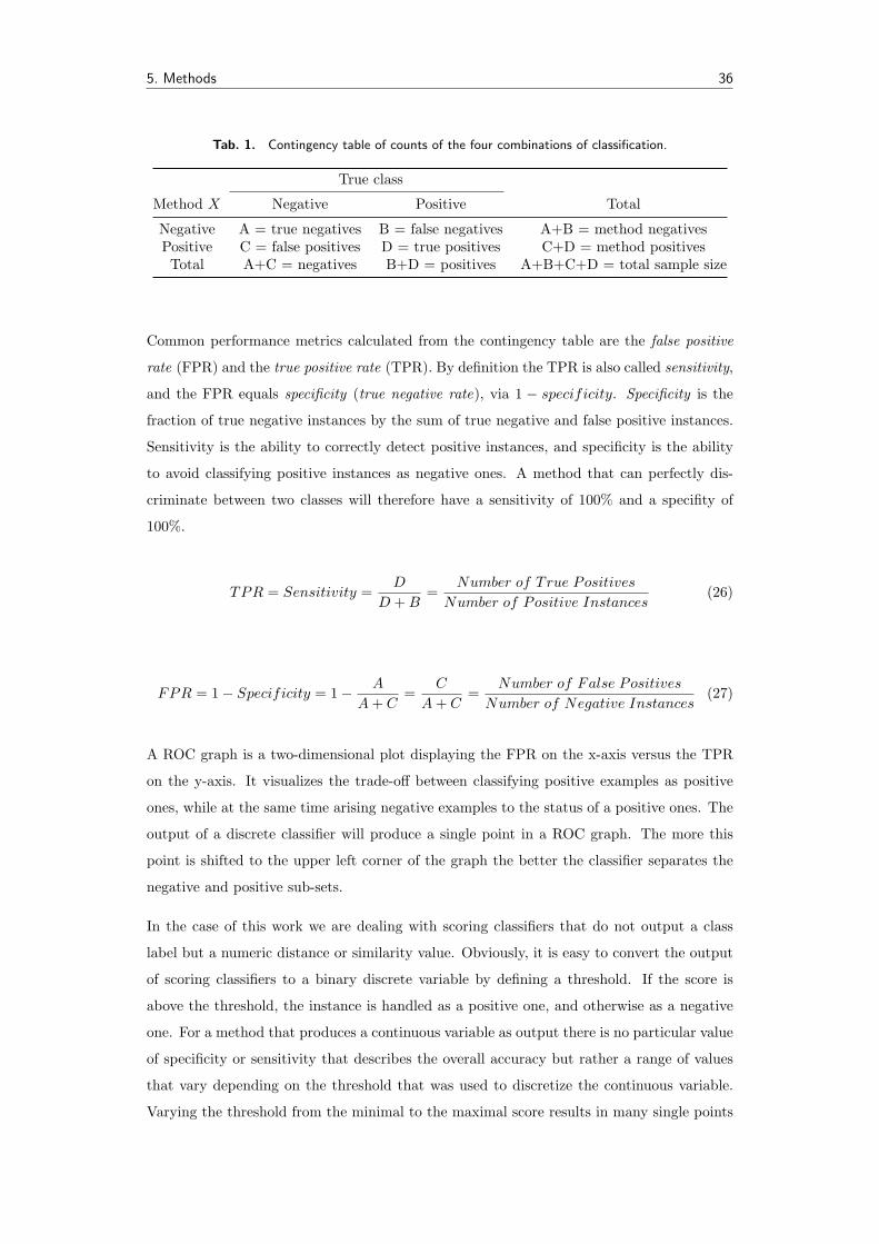
5. Methods 36
Tab. 1. Contingency table of counts of the four combinations of classification.
True class
Method X Negative Positive Total
Negative A = true negatives B = false negatives A+B = method negativesPositive C = false positives D = true positives C+D = method positivesTotal A+C = negatives B+D = positives A+B+C+D = total sample size
Common performance metrics calculated from the contingency table are the false positive
rate (FPR) and the true positive rate (TPR). By definition the TPR is also called sensitivity,
and the FPR equals specificity (true negative rate), via 1 − specificity. Specificity is the
fraction of true negative instances by the sum of true negative and false positive instances.
Sensitivity is the ability to correctly detect positive instances, and specificity is the ability
to avoid classifying positive instances as negative ones. A method that can perfectly dis-
criminate between two classes will therefore have a sensitivity of 100% and a specifity of
100%.
TPR = Sensitivity =D
D + B=
Number of True Positives
Number of Positive Instances(26)
FPR = 1− Specificity = 1− A
A + C=
C
A + C=
Number of False Positives
Number of Negative Instances(27)
A ROC graph is a two-dimensional plot displaying the FPR on the x-axis versus the TPR
on the y-axis. It visualizes the trade-off between classifying positive examples as positive
ones, while at the same time arising negative examples to the status of a positive ones. The
output of a discrete classifier will produce a single point in a ROC graph. The more this
point is shifted to the upper left corner of the graph the better the classifier separates the
negative and positive sub-sets.
In the case of this work we are dealing with scoring classifiers that do not output a class
label but a numeric distance or similarity value. Obviously, it is easy to convert the output
of scoring classifiers to a binary discrete variable by defining a threshold. If the score is
above the threshold, the instance is handled as a positive one, and otherwise as a negative
one. For a method that produces a continuous variable as output there is no particular value
of specificity or sensitivity that describes the overall accuracy but rather a range of values
that vary depending on the threshold that was used to discretize the continuous variable.
Varying the threshold from the minimal to the maximal score results in many single points

5. Methods 37
in the ROC space that capture the trade-off between sensitivity and specificity of a method
over the entire range. These points can be joined to form an empirical ROC curve. A
ROC curve for a method with perfect accuracy would run vertically from the point (0, 0)
to the upper left corner and then horizontally to the point (1, 1). Random guessing would
correspond to a diagonal from point (0, 0) to (1, 1). Fig. 16 shows two sample ROC graphs
and histograms for positive and negative populations at different levels of overlap.
False positive rate
Tru
e po
sitiv
e ra
te
0.0 0.2 0.4 0.6 0.8 1.0
0.0
0.2
0.4
0.6
0.8
1.0
0.0 0.2 0.4 0.6 0.8 1.0 1.2
050
100
150
200
250
300
SCI
Fre
quen
cy
False positive rate
Tru
e po
sitiv
e ra
te
0.0 0.2 0.4 0.6 0.8 1.0
0.0
0.2
0.4
0.6
0.8
1.0
0.0 0.2 0.4 0.6 0.8 1.0 1.2
050
100
150
200
250
300
SCI
Fre
quen
cy
Fig. 16. Sample ROC graphs for a scoring classifier in combination with histograms of thenegative and positive instances. The more the curve is shifted to the upper left corner thebetter the overall performance of the classifier is in a way that the two populations can beseparated from each other.
While ROC graphs are useful for visually assessing the accuracy of a method, for many
purposes a single index summarizing a ROC curve is desired. The full area under the ROC
curve (AUC) is a suitable single scalar value representing the overall accuracy of a method.
It has several interpretations: (i) the probability that a randomly drawn positive instance
will have a higher score than a randomly drawn negative example, (ii) the average sensitivity
over all values of specificity, and (iii) the average specificity over all values of sensitivity. The
AUC varies from 0.5 which equals random guessing to 1.0 indicating perfect discrimination
power. As outlined before, an empirical ROC curve can be constructed simply by joining

5. Methods 38
single values in the ROC space but this will result in a jagged curve which is only an
approximation to the true, continuous ROC curve. A simple method to calculate the area
under the empirical ROC curve is by using the trapezoid rule. The AUC calculated this
way is equivalent to other statistics like the Mann-Whitney U statistic or the Wilcoxon rank
sum statistic. This equivalence allows to calculate confidence intervals and standard errors
(Hanley & McNeil, 1982). DeLong et al. (1988) provide a strategy to statistically assess
the significance of the difference of two AUC values derived from the same set of instances.
The main advantage of the empirical method over parametric approaches, which calculate
the area under a smoothed ROC curve, is that there are no structural assumptions on the
data.
Sample size planing for ROC analysis is a complex field. There are strategies for efficient
sample size determination for two given AUC values at a predefined type I error and statis-
tical power, but as this study considers several hundred AUC values this turns out to be a
difficult task. We follow the strategy proposed by Hanley & McNeil (1982) to determine a
minimal sample size based on the magnitude of the standard error. To determine whether
two AUC values differ significantly we use then the asymptotic non-parametric method by
DeLong et al. (1988).
By varying the sample size and plotting the resulting standard error (SE) one can visually
choose a sample size that has a suitable small standard error. Instances are randomly
selected from a larger population with known empirical AUC values for the SCI as classifier.
AUC values are then calculated for a given sample size. Fig. 17 illustrates the results. Even
though lower AUC values are expected in the analysis, a minimal sample size of 200 positive
and 200 negative instances seems to yield reasonable results, as the relative gain in a lower
SE is small when moving to a higher sample size.
In this study all AUC values are derived by averaging over AUC values from comparison
of the native alignments to each of the five random control alignment populations. For
ROC graph generation and AUC calculations the software package R (R Development Core
Team, 2006) version 2.4.1 with the package ROCR (Sing et al., 2005) for classifier performance
evaluation was used.
5.3 Shannon entropy as a measure of sequence variation in an alignment
Evolutionary information in the form of an alignment of related sequences is provided in two
ways: (i) sequence variation, i.e. possible consistent and compensatory mutations, and (ii)
number of sequences. The more sequences that are able to form a particular base-pair, the
more evidence is given that the base-pair may be correct. In order to do adequate measuring

5. Methods 39
0 100 200 300 400
0.00
0.02
0.04
0.06
0.08
0.10
0.12
Standard Error for Area Under ROC curves
Sample size (positive examples)
Sta
ndar
d E
rror
AUC ~ 0.80AUC ~ 0.89AUC ~ 0.97
Fig. 17. Standard error (SE) in relation to the sample size of positive instances (with equalnumber of negative instances). A sample size of 200 positive and 200 negative instancesseems to be a reasonable minimal threshold.
of the discrimination capability of a method it is necessary to divide the data set into subsets
grouped by the content of information they hold.
A common measure describing sequence variation in a multiple sequence alignment is the
average pairwise sequence identity (API). There are various ways for computing this measure
but in this work we stick to the version where a gap-nucleotide pair is treated as a mismatch.
Therefore, the pairwise distance between two sequences is simply the hamming distance
divided by the number of columns. Although this measure is widely used, it is only capable
of assessing sequence variation, and does not take the number of sequences that constitute
the alignment into account. If one intends to create subsets by splitting by the API, it
would be necessary to subdivide these data sets again by the number of sequences in the
alignment.
A way to overcome this problem, is to use a measure that is capable of assessing both
sequence variation and the number of sequences. For this purpose the normalized Shannon
entropy (H) can be used. As this measure comes initially from the field of information
theory it is generally referred to as the average minimum number of bits needed to encode
a string based on the frequency of the symbols. In our case we are dealing with an alphabet
Σ = {A,C, G, T,−} composed of the four nucleotides plus the gap character “-”. The

5. Methods 40
probabilities are approximated by frequencies, e.g. piA is the frequency of the character A
in column i divided by the number of sequences in the alignment. The normalized Shannon
entropy of an alignment A is defined by the sum of the Shannon entropies of the individual
columns divided by the length of the alignment denoted by |A|.
H = − 1|A|
|A|∑
i
∑
j∈Σ
pij log2 pi
j (28)
In the case of two sequences the normalized Shannon entropy equals the pairwise sequence
identity via:
API = 1−H (29)
For alignments with more than two sequences it is not straightforward to express the API
by the normalized Shannon entropy and vice versa. Nevertheless, these two measures are
highly correlated as shown in Fig. 18.
0.0 0.2 0.4 0.6 0.8 1.0 1.2 1.4
3040
5060
7080
9010
0
normalized Shannon entropy
aver
age
pairw
ise
sequ
ence
iden
tity
2 Sequences3 Sequences5 Sequences7 Sequences10 Sequences15 Sequences
Fig. 18. Relation between the average pairwise sequence identity and the normalized Shannonentropy. Lines were derived by linear regression from the BRAliBase 2.1 data set using thestatistical software package R. All regressions yielded a R squared higher than 0.99.
For the generation of subsets that are subsequently subjected to ROC analysis a bin size
of 0.05 was chosen. An overview of the composition of the resulting sub-data sets for the

5. Methods 41
Bralibase 2.1 and CLUSTAL W data sets are show in Fig. 19 and 20. According to the
findings of the minimal sample size selection process only bins with more than 200 positive
instances are considered for further analysis.
0.05 0.10 0.15 0.20 0.25 0.30 0.35 0.40 0.45 0.50 0.55 0.60 0.65 0.70 0.75 0.80 0.85 0.90 0.95 1.00 1.05 1.10 1.15 1.20 1.25 1.30 1.35 1.40 1.45
Normalized Shannon Entropy in bins with bin size of 0.05
Fre
quen
cy
050
010
0015
0020
00
0
1019
1463
1891
1596
1310
918
797
873903
11511211
923866
584547
519
429
355409
335
259228
184
11365
337 2
2 Sequences3 Sequences5 Sequences7 Sequences10 Sequences15 Sequences
Fig. 19. Bar chart indicating the number of positive instances in the BRAliBase 2.1 dataset in every bin. The red line indicates the minimal threshold of positive instances to givereasonable results in an ROC analysis.

5. Methods 42
0.05 0.10 0.15 0.20 0.25 0.30 0.35 0.40 0.45 0.50 0.55 0.60 0.65 0.70 0.75 0.80 0.85 0.90 0.95 1.00 1.05 1.10 1.15 1.20 1.25 1.30 1.35 1.40 1.45 1.50 1.55
Normalized Shannon Entropy in bins with bin size of 0.05
Fre
quen
cy
050
010
0015
0020
00
22
1085
1512
1972
1632
1314
959
887
1020
1115
1351
1084
812
623
481440
414 403
308279
246 242212 191
136110
7438 21 5 2
2 Sequences3 Sequences5 Sequences7 Sequences10 Sequences15 Sequences
Fig. 20. Bar chart indicating the number of positive instances in the CLUSTAL W data set inevery bin. The red line indicates the minimal threshold of positive instances to give reasonableresults in an ROC analysis.
Pairwise alignments constitute a overwhelming majority in some of the bins. To exclude the
possibility that results are just artefacts of an excess of pairwise alignments, we calculated
AUC values for bins with the maximal number of pairwise alignments being at most the
number of three-way alignments. For the reduced data set pairwise alignments were selected
randomly. AUC values may vary slightly, but general trends are preserved. Results on
CLUSTAL W generated alignments for the SCI and the pairwise comparison approach using
RNAeval are shown in Tab. 4 in appendix A.

6. Measuring evolutionary conservation: results and discussion 43
6 Measuring evolutionary conservation: results and discus-
sion
Performance of the various methods for assessing structural conservation was tested on
structural alignments of the BRAliBase 2.1 data set and on sequence alignments generated
by realigning BRAliBase 2.1 with CLUSTAL W. For subsequent ROC analysis, alignments
were binned according to their Shannon entropy. The Shannon entropy as a measure of the
average information content does not only take sequence variation into account, but also
the number of sequences that constitute the alignment. Low entropy means low information
content, i.e. there is not much sequence variation that can give rise to possible compen-
satory mutations. The normalized Shannon entropy is inversely proportional to the average
pairwise identity. Hence, low entropy corresponds to a high average pairwise identity, which
means high sequence conservation.
This study evaluates classification power in two ways: (i) for each bin with more than 200
alignments the area under the ROC curve (AUC) will be presented, and (ii) the sensitivity
of a method at a fixed specificity of 95% is examined for three predefined intervals (low,
medium, and high entropy range).
6.1 Minimum free energy based methods
Both the SCI and the pairwise approach using RNAeval quantify structural conservation
in terms of energy, rather than considering secondary structures themselves. A detailed
discussion of minimum free energy based methods is given in section 4.1. Results are shown
in Fig. 22 for the structural data set and in Fig. 23 for the CLUSTAL W generated data set.
In general, the SCI can be calculated by two ways. Either dividing the consensus energy by
the mean of the energies of the native sequences with gaps removed or including gap char-
acters. Although this will yield different SCI values for single instances, it does not shown a
significant effect on the discrimination capability of the two variants on both structural and
CLUSTAL W generated alignments. A general trend that can be noticed is that the covariance
scoring model of the RNAalifold algorithm significantly improves the discrimination power
in most cases. The gain in accuracy is best shown in the medium entropy range of the
structural alignment data set (all p-values < 0.001). The additional negative bonus energy
for compensatory and/or consistent mutations involve a shift of the SCI to higher values,
which therefore causes a better separation between positive and negative instances. In the
low entropy range there is little covariance information which can be exploited and hence the

6. Measuring evolutionary conservation: results and discussion 44
SCI with and without covariance model show equal performance. A series of empirical ROC
curves for the SCI is shown in Fig. 21. ROC curves for structural alignments are shifted
more to the upper left corner with increasing entropy indicating better discrimination power.
For CLUSTAL W generated alignments this trend is nearly inverted, as the alignment quality
with regard to RNA secondary structure drops with increasing entropy. As this method of
visualization soon becomes unmanageable, we will stick to graphs representing AUC values
at given entropy bins for subsequent analysis. However, one has to keep in mind that the
reduction of a ROC curve to a single scalar value comes along with a loss of information.
0.05 − 0.10
0.0
0.2
0.4
0.6
0.8
1.0
0.10 − 0.15 0.15 − 0.20 0.20 − 0.25
0.25 − 0.30
0.0
0.2
0.4
0.6
0.8
1.0
0.30 − 0.35 0.35 − 0.40 0.40 − 0.45
0.45 − 0.50
0.0
0.2
0.4
0.6
0.8
1.0
0.50 − 0.55 0.55 − 0.60 0.60 − 0.65
0.65 − 0.70
0.0 0.2 0.4 0.6 0.8 1.0
0.0
0.2
0.4
0.6
0.8
1.0
0.70 − 0.75
0.0 0.2 0.4 0.6 0.8 1.0
0.75 − 0.80
0.0 0.2 0.4 0.6 0.8 1.0
0.80 − 0.85
0.0 0.2 0.4 0.6 0.8 1.0
Fig. 21. Empirical ROC curves for the SCI for different entropy bins on structural alignments(black) and CLUSTAL W generated alignments (red). On structural alignments the SCI gainsin discrimination capability with increasing entropy. At an entropy range of 0.80 and abovesufficient information is contained in the alignments to perfectly separate truly conservedinstances from randomizes ones. On CLUSTAL W generated alignments the discriminationcapability of the SCI drops with increasing entropy, as the alignment quality with regard tosecondary structure becomes worse.
As CLUSTAL W produces alignments solely based on the information contained in the nu-
cleotide sequence and does not take RNA secondary structures into account, results are
expected to become worse for those methods that somehow depend on the quality of the

6. Measuring evolutionary conservation: results and discussion 45
AU
C
0.5
0.6
0.7
0.8
0.9
1.0
0.05 0.10 0.15 0.20 0.25 0.30 0.35 0.40 0.45 0.50 0.55 0.60 0.65 0.70 0.75 0.80 0.85 0.90 0.95 1.00 1.05 1.10
normalized Shannon entropy
low entropy medium entropy high entropy
SCI with gapsSCI without gapsSCI without covariance modelRNAeval,pairwise
Fig. 22. Comparison of minimum free energy methods on structural alignments. The twoSCI variants (calculation of single minimum free energies on sequences with and withoutgap characters) are indistinguishable in their performance. The SCI without the RNAalifold
covariance model performs significantly worse than the two other SCI variants. The pair-wise comparison approach using RNAeval performs only on alignments with highly conservedsequences better.
alignment. Especially, at a low average pairwise identity the chance that compensatory and
consistent mutations, which are absolutely mandatory to achieve “good” consensus structure
predictions, are aligned the right way is low2. The first downward trend of the SCI ranging
from an entropy level of 0.30 to 0.60 is caused by prevalence of pairwise alignments with
low sequence identity. An average pairwise identity of 60% to 65% or below is considered as
critical with regard to secondary structures for alignments generated solely on sequence in-
formation. This results in a relatively low discrimination capability of the SCI in this region.
As soon as low identity pairwise alignments do not constitute the majority of instances in a
bin, the predictive power of the SCI raises again. The second performance drop of the SCI
in the entropy range of 0.75 to 0.90 is again caused by prevalence of alignments with low
sequence identity, in this case alignments with three sequences.
The pairwise comparison approach using RNAeval performs significantly better on align-
ments with low Shannon entropy (range from 0.05 to 0.15 with p-values < 0.001) than the
SCI. Since we are dealing with methods that consider energies of RNA secondary structures
and not secondary structures themselves it is not trivial to interpret the better performance2As the performance of the SCI strictly depends on the quality of the alignments, the SCI has hence been
used as a general measure of the alignment quality with regard to RNA secondary structure (Wilm et al.,2006).

6. Measuring evolutionary conservation: results and discussion 46
of the RNAeval approach on alignments with highly conserved sequences. But the RNAeval
approach seems to be more sensitive in evaluating the small nuances of secondary structures
changes at this high level of conservation. The SCI and the RNAeval approach operate on
two different scales. While the SCI is bounded below by 0, the RNAeval approach is bounded
above by 1, which causes favoring of two extreme cases. In the case of the SCI an align-
ment with loads of compensatory and consistent mutations will yield a SCI above 1 due to
negative bonus energies. The RNAeval approach will give at most 1 as compensatory and
consistent mutations are not specially rewarded. In the case of an alignment of sequences
that do not share a common fold the SCI will be 0, while the RNAeval approach will yield
a value below 0 as the evaluation of a sequence forced to fold into a structure that is not
likely to be adopted by that sequence will give positive energy values. Hence, in the case of
the SCI we are dealing with a better dispersion of positive examples, and vice versa in the
RNAeval approach with a better dispersion of negative examples.
AU
C
0.5
0.6
0.7
0.8
0.9
1.0
0.05 0.10 0.15 0.20 0.25 0.30 0.35 0.40 0.45 0.50 0.55 0.60 0.65 0.70 0.75 0.80 0.85 0.90 0.95 1.00 1.05 1.10
normalized Shannon entropy
low entropy medium entropy high entropy
SCI with gapsSCI without gapsSCI without covariance modelRNAeval,pairwise
Fig. 23. Comparison of minimum free energy methods on CLUSTAL W generated alignments.The up and down movements of the SCI variants are caused by the alignment quality withregard to RNA secondary structure. The first downward trend is caused by pairwise alignmentswith low sequence identity, the second by three-way alignments with low sequence identity.SCI variants with covariance model perform significantly better than the version that does notmake use of covariance information. The pairwise comparison approach using RNAeval showshigher discrimination capability than the SCI methods on alignments with highly conservedsequences.

6. Measuring evolutionary conservation: results and discussion 47
6.2 Methods based on base-pair distances
The base-pair distance allows pairwise comparison of RNA secondary structures by comput-
ing the symmetric set difference of base-pairs of two structures. However, this method can
be easily extended to compare ensembles of structures derived from the individual sequences.
A detailed discussion of these methods including limitations is given in section 4.3. Results
are shown in Fig. 24 for the structural data set and in Fig. 25 for the CLUSTAL W generated
data set.
The base-pair distance is one of the simplest measures on a set of secondary structures that
can be defined. In contrast to the SCI that is abstracting of structure, the base-pair distance
is sensitive to the exact positions of the base-pairs. Hence, the alignment quality will have
great influence on the results. On the structural alignment data set, with exception of the
low entropy range the SCI shows higher discrimination power than the base-pair distance
methods. As seen above for the pairwise RNAeval approach, the pairwise base-pair distance
approach shows also higher discrimination capability in the low entropy range than the
approach using the base-pair distance to the consensus structure. One has to keep in mind
that the randomized negatives examples were generated by shuffling of the corresponding
positive ones. On alignments with low entropy, sequences are nearly identical and hence
RNAalifold is likely to find a good consensus structure for the negative instances, too.
The pairwise comparison approach seems to be better suited to catch the small differences
in structures at this high level of conservation. As soon as more information in form of
sequence variation or number of sequences that give evidence that a single base-pair may
be correct is given, the consensus approach gains on discrimination power over the pairwise
approach, on both structural and CLUSTAL W generated alignments. The consensus base-pair
distance follows strictly the trend of the SCI, but shows higher discrimination power and is
less sensitive to alignment errors than the SCI on CLUSTAL W generated alignments.
The ensemble base-pair distance methods perform moderately on structural alignments, but
show only little or no discrimination capability on CLUSTAL W generated alignments. The bad
performance of the consensus approach can be explained by considering the way base-pairing
probabilities are generated. In the case of a single sequence there are no special rules for two
bases to form a base-pair, they just have to belong to the set of valid base-pairs. RNAfold
can therefore assign to each valid base-pair a base-pairing probability. On the alignment
level this is more complicated as we are dealing with columns of nucleotides rather than
with single nucleotides. In the RNAalifold algorithm, only those column pairs in which at
least 50% of the sequences can form a base-pair are allowed to enter computation. In the
case of the consensus comparison approach there may be many base-pairing probabilities in

6. Measuring evolutionary conservation: results and discussion 48
the single sequences that do not have a consensus counterpart to subtract, which results in
an addition of the full probability to the distance. Another point that greatly influences the
performance of the ensemble distance methods is that each probability of each possible base-
pair of one structure is compared to the corresponding probability of the other structure or
the consensus structure and therefore these methods are extremely sensitive to the alignment
quality.
AU
C
0.5
0.6
0.7
0.8
0.9
1.0
0.05 0.10 0.15 0.20 0.25 0.30 0.35 0.40 0.45 0.50 0.55 0.60 0.65 0.70 0.75 0.80 0.85 0.90 0.95 1.00 1.05 1.10
normalized Shannon entropy
low entropy medium entropy high entropy
SCIconsensuspairwiseconsensus,ensemblepairwise,ensemble
Fig. 24. Comparison of base-pair distance based methods on structural alignments. In the lowentropy range the pairwise base-pair distance approach shows higher discrimination capabilitythan its consensus structure counterpart or the SCI. As soon as more information in formof sequence variation or number of sequences is available the consensus approach gains ondiscrimination capability over the pairwise approach. Ensemble base-pair distance methodsshow only moderate performance.
6.3 Tree editing methods
In this study we considered various tree representations of RNA secondary structures and
enhanced structure comparison concepts such as MiGaL. A detailed discussion of tree rep-
resentations and tree editing is given in section 3.2.2 and section 4.2, respectively. For the
full, HIT, coarse-grained, and weighted coarse-grained tree representations we report results
on both pairwise comparisons shown in Fig. 28 and 29, and on comparisons of single se-
quences of an alignment to the consensus secondary structure, shown in Fig. 26 and 27. For
the HIT representation we present combined results of all approaches on both structural
and CLUSTAL W generated alignments in Fig. 30. As the MiGaL algorithm makes use of the
nucleotide sequence, we considered only pairwise comparisons and report results on all four

6. Measuring evolutionary conservation: results and discussion 49
AU
C
0.3
0.4
0.5
0.6
0.7
0.8
0.9
1.0
0.05 0.10 0.15 0.20 0.25 0.30 0.35 0.40 0.45 0.50 0.55 0.60 0.65 0.70 0.75 0.80 0.85 0.90 0.95 1.00 1.05 1.10
normalized Shannon entropy
low entropy medium entropy high entropy
SCIconsensuspairwiseconsensus,ensemblepairwise,ensemble
Fig. 25. Comparison of base-pair distance based methods on CLUSTAL W generated align-ments. The pairwise base-pair distance approach shows better performance in the low en-tropy range than the consensus approach or the SCI. As soon as more information is availablethat can be exploited by the RNAalifold algorithm for more confident consensus structureprediction the consensus approach gains on discrimination power. As both methods are alsosensitive to the alignment quality the follow the trend of the SCI, but show more resistance toalignment errors and a slightly better or equal performance than the SCI. Ensemble base-pairmethods show only little or no discrimination capability.

6. Measuring evolutionary conservation: results and discussion 50
layer models of the MiGaL concept in Fig. 31 and 32.
None of the various tree editing approaches shows a discrimination capability between truly
conserved RNA secondary structures and randomized instances as high as the SCI over the
whole spectrum of the alignment data sets used for investigation.
Comparison of secondary structures of the single sequences of an alignment to the consensus
secondary structure makes use of the same principle as the SCI does. If sequences are
evolutionary related and belong to the same structural family, RNAalifold should be able to
compute a consensus secondary structure that can be adopted by all these sequences. Hence,
the secondary structures of the single sequences should have a low tree editing distance to
the consensus structure. In the case of non related sequences RNAalifold will output in
general a secondary structure with only few structural elements or even the open chain.
Because of that distances of the secondary structures of the individual sequences to the
consensus structure should be high. As a consequence of this, results strictly follow the
trends of the SCI on both structural and CLUSTAL W generated alignments but we observe
much less discrimination capability than the SCI.
AU
C
0.5
0.6
0.7
0.8
0.9
1.0
0.05 0.10 0.15 0.20 0.25 0.30 0.35 0.40 0.45 0.50 0.55 0.60 0.65 0.70 0.75 0.80 0.85 0.90 0.95 1.00 1.05 1.10
normalized Shannon entropy
low entropy medium entropy high entropy
SCIfullHITweighted coarse−grainedweighted coarse−grained, Shapirocoarse−grainedcoarse−grained, Shapiro
Fig. 26. Comparison of tree editing distance methods for single sequences to the consensus se-quence for various tree representations of RNA secondary structures on structural alignments.The full and HIT representation, that maintain full information encoded in a secondary struc-ture, perform significantly better than representations that are abstracting of structural detail.
In general, the full and the HIT representation have the highest discrimination power over
other representations that are abstracting of structural details. The loss of detailed struc-
tural information as in the case of the coarse-grained representation leads also to a loss in

6. Measuring evolutionary conservation: results and discussion 51
AU
C
0.5
0.6
0.7
0.8
0.9
1.0
0.05 0.10 0.15 0.20 0.25 0.30 0.35 0.40 0.45 0.50 0.55 0.60 0.65 0.70 0.75 0.80 0.85 0.90 0.95 1.00 1.05 1.10
normalized Shannon entropy
low entropy medium entropy high entropy
SCIfullHITweighted coarse−grainedweighted coarse−grained, Shapirocoarse−grainedcoarse−grained, Shapiro
Fig. 27. Comparison of tree editing distance methods for single sequences to the consensussequence for various tree representations of RNA secondary structures on CLUSTAL W generatedalignments. All methods follow strictly the trend of the SCI. There is again the trend that themore information is encoded by a tree representation, the better the discrimination capabilityis.
discrimination power, which can be easily demonstrated on an example from the Bralibase
2.1 data set. We use RNAfold to calculate the MFE structures of two Hammerhead 3 se-
quences, which have a general structural motif that is composed of three base-paired helices
separated by short linkers. In addition, we calculate the MFE structures of two randomized
instances of the native sequences.
native Sequence 1 .(((((((((((((....))))))).......((((....))))...)))))).
native Sequence 2 (((((((((((((....))))........(((((......))))).)))))))))
rand. Sequence 1 ((((((((.......)))))))).((.(((.((((.....))))))).))....
rand. Sequence 2 .........((..........))..(((..(((((((....))))..)))..)))
Just by visual examination one would rate the set of native sequences to be related or
to have a small distance in some metric space, while the randomized sequences would be
considered to be quite distinct to each other. In the coarse-grained representations the two
native sequences share the same structural motif (HSHSMSR), but also the two randomized
sequences have the same structural coarse-grained representation (HSHSBSISR) (for details
on coarse-grained tree representation see section 3.2.2). Therefore, both sets would have a
distance of 0 in the coarse-grained representation. The weighted coarse-grained approach

6. Measuring evolutionary conservation: results and discussion 52
maintains a higher level of structural information than the coarse-grained representation and
performs therefore in general better. The use of different costs for the tree editing operations
has significant influences on the discrimination power of the methods. Tree editing distance
of the coarse-grained and weighted coarse-grained representations were calculated using
the cost matrix of Vienna RNA package and the costs initially proposed by Shapiro. In
general, the weighted coarse-grained approach using the Vienna RNA package costs performs
significantly better or at least equal on both structural and CLUSTAL W generated alignments
than the weighted coarse-grained approach using Shapiro’s costs. This trend cannot be
demonstrated that clearly on the coarse-grained representation.
AU
C
0.5
0.6
0.7
0.8
0.9
1.0
0.05 0.10 0.15 0.20 0.25 0.30 0.35 0.40 0.45 0.50 0.55 0.60 0.65 0.70 0.75 0.80 0.85 0.90 0.95 1.00 1.05 1.10
normalized Shannon entropy
low entropy medium entropy high entropy
SCIfullHITweighted coarse−grainedweighted coarse−grained, Shapirocoarse−grainedcoarse−grained, Shapiro
Fig. 28. Comparison of tree editing distance for pairwise evaluations of various tree rep-resentations of RNA secondary structures on structural alignments. The hierarchy of treerepresentation on the discrimination capability is equal to that observed at the tree editingmethods using a consensus secondary structure. The more structural information a repre-sentation is able to present, the better the discrimination power is. In general, the pairwiseapproach shows a significant drop in discrimination capability compared to the equivalentmethods that make use of a consensus structure.
Tree editing is also suited for comparing sequences of different length. We investigate this
strategy also for the HIT representation, summarized results for all approaches for the
HIT representation are shown in Fig. 30. On structural alignments, the approach using
a consensus structure performs better than all the other pairwise comparison approaches.
The pairwise comparison approach on structural alignments and the pairwise comparison
approach on sequences without gap characters show equal performance and both perform
better than the pairwise comparison approach on CLUSTAL W generated alignments. Hence,
on alignments with low quality with regard to secondary structure, it seems to be a good
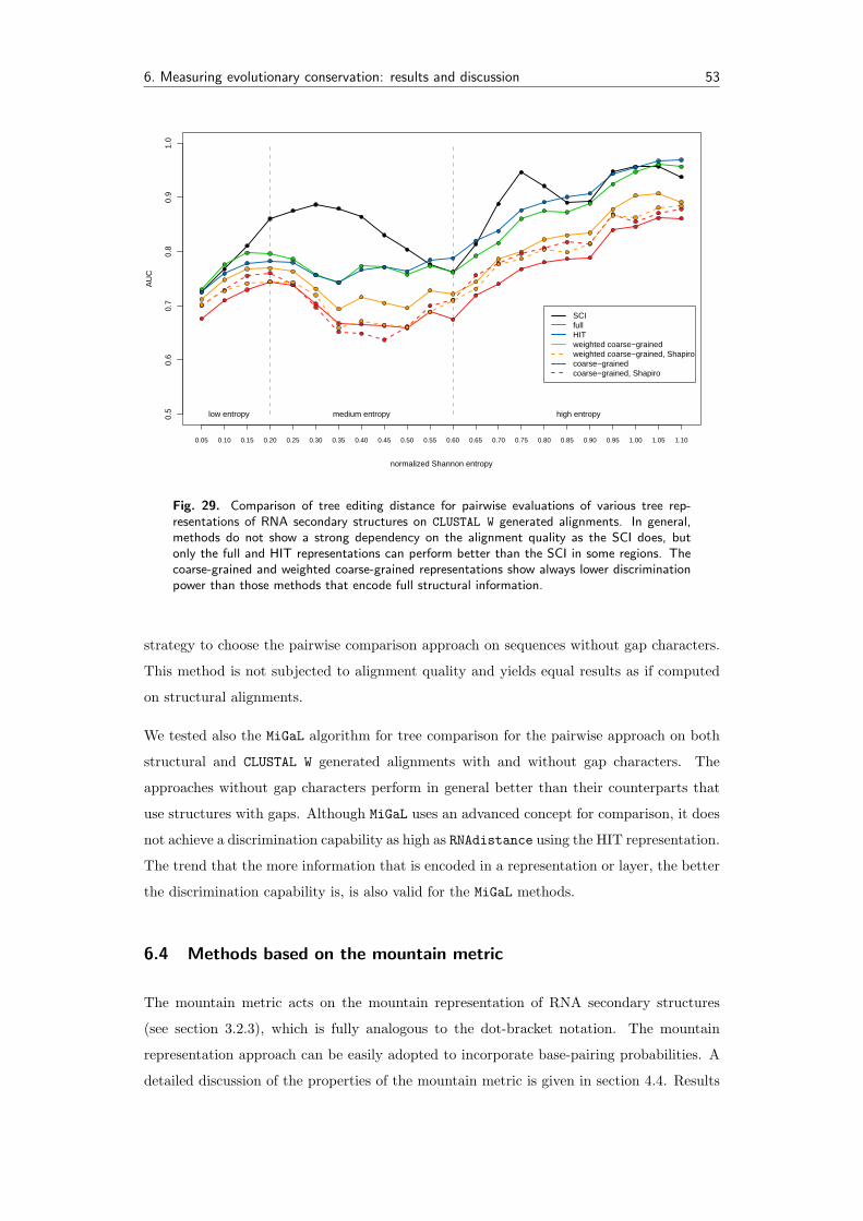
6. Measuring evolutionary conservation: results and discussion 53
AU
C
0.5
0.6
0.7
0.8
0.9
1.0
0.05 0.10 0.15 0.20 0.25 0.30 0.35 0.40 0.45 0.50 0.55 0.60 0.65 0.70 0.75 0.80 0.85 0.90 0.95 1.00 1.05 1.10
normalized Shannon entropy
low entropy medium entropy high entropy
SCIfullHITweighted coarse−grainedweighted coarse−grained, Shapirocoarse−grainedcoarse−grained, Shapiro
Fig. 29. Comparison of tree editing distance for pairwise evaluations of various tree rep-resentations of RNA secondary structures on CLUSTAL W generated alignments. In general,methods do not show a strong dependency on the alignment quality as the SCI does, butonly the full and HIT representations can perform better than the SCI in some regions. Thecoarse-grained and weighted coarse-grained representations show always lower discriminationpower than those methods that encode full structural information.
strategy to choose the pairwise comparison approach on sequences without gap characters.
This method is not subjected to alignment quality and yields equal results as if computed
on structural alignments.
We tested also the MiGaL algorithm for tree comparison for the pairwise approach on both
structural and CLUSTAL W generated alignments with and without gap characters. The
approaches without gap characters perform in general better than their counterparts that
use structures with gaps. Although MiGaL uses an advanced concept for comparison, it does
not achieve a discrimination capability as high as RNAdistance using the HIT representation.
The trend that the more information that is encoded in a representation or layer, the better
the discrimination capability is, is also valid for the MiGaL methods.
6.4 Methods based on the mountain metric
The mountain metric acts on the mountain representation of RNA secondary structures
(see section 3.2.3), which is fully analogous to the dot-bracket notation. The mountain
representation approach can be easily adopted to incorporate base-pairing probabilities. A
detailed discussion of the properties of the mountain metric is given in section 4.4. Results
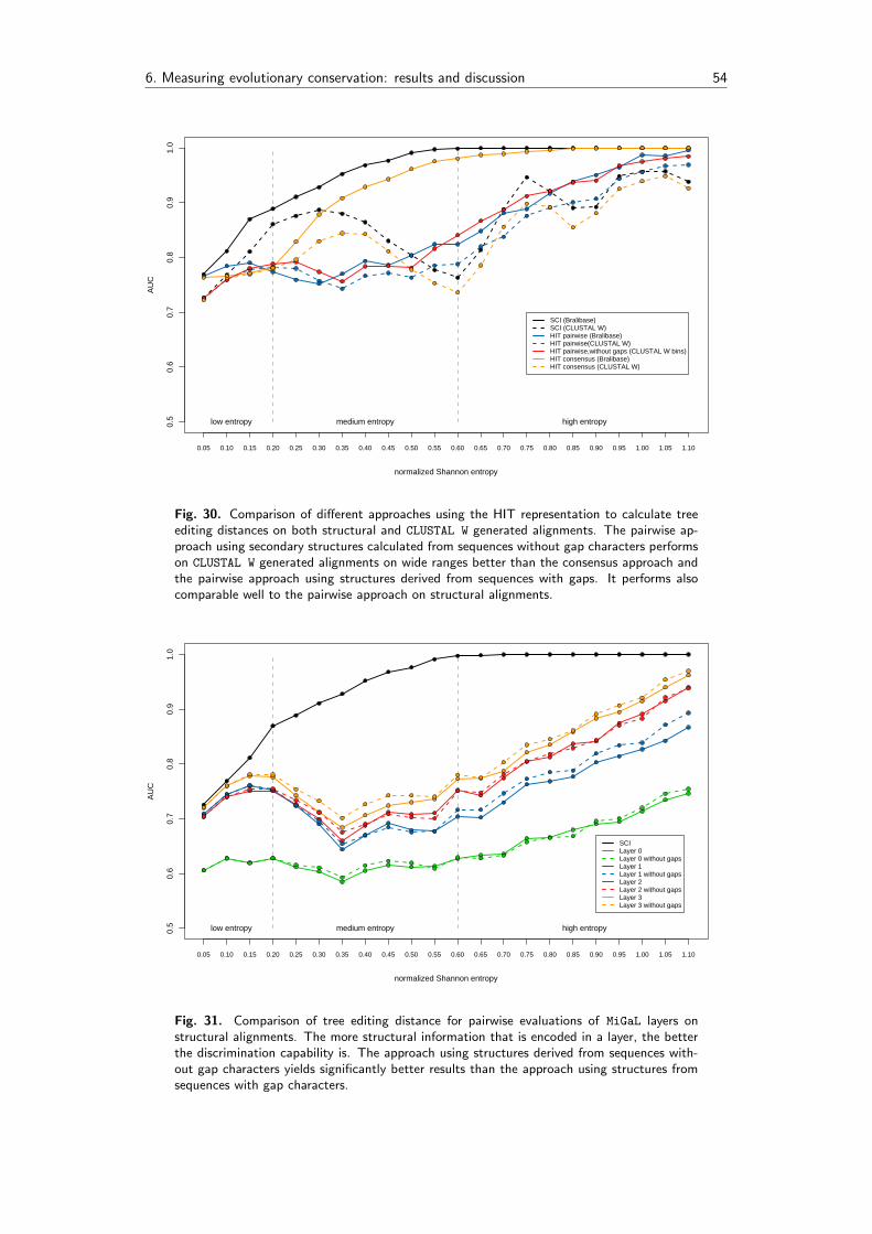
6. Measuring evolutionary conservation: results and discussion 54
AU
C
0.5
0.6
0.7
0.8
0.9
1.0
0.05 0.10 0.15 0.20 0.25 0.30 0.35 0.40 0.45 0.50 0.55 0.60 0.65 0.70 0.75 0.80 0.85 0.90 0.95 1.00 1.05 1.10
normalized Shannon entropy
low entropy medium entropy high entropy
SCI (Bralibase)SCI (CLUSTAL W)HIT pairwise (Bralibase)HIT pairwise(CLUSTAL W)HIT pairwise,without gaps (CLUSTAL W bins)HIT consensus (Bralibase)HIT consensus (CLUSTAL W)
Fig. 30. Comparison of different approaches using the HIT representation to calculate treeediting distances on both structural and CLUSTAL W generated alignments. The pairwise ap-proach using secondary structures calculated from sequences without gap characters performson CLUSTAL W generated alignments on wide ranges better than the consensus approach andthe pairwise approach using structures derived from sequences with gaps. It performs alsocomparable well to the pairwise approach on structural alignments.
AU
C
0.5
0.6
0.7
0.8
0.9
1.0
0.05 0.10 0.15 0.20 0.25 0.30 0.35 0.40 0.45 0.50 0.55 0.60 0.65 0.70 0.75 0.80 0.85 0.90 0.95 1.00 1.05 1.10
normalized Shannon entropy
low entropy medium entropy high entropy
SCILayer 0Layer 0 without gapsLayer 1Layer 1 without gapsLayer 2Layer 2 without gapsLayer 3Layer 3 without gaps
Fig. 31. Comparison of tree editing distance for pairwise evaluations of MiGaL layers onstructural alignments. The more structural information that is encoded in a layer, the betterthe discrimination capability is. The approach using structures derived from sequences with-out gap characters yields significantly better results than the approach using structures fromsequences with gap characters.

6. Measuring evolutionary conservation: results and discussion 55
AU
C
0.5
0.6
0.7
0.8
0.9
1.0
0.05 0.10 0.15 0.20 0.25 0.30 0.35 0.40 0.45 0.50 0.55 0.60 0.65 0.70 0.75 0.80 0.85 0.90 0.95 1.00 1.05 1.10
normalized Shannon entropy
low entropy medium entropy high entropy
SCILayer 0Layer 0 without gapsLayer 1Layer 1 without gapsLayer 2Layer 2 without gapsLayer 3Layer 3 without gaps
Fig. 32. Comparison of tree editing distance for pairwise evaluations of MiGaL layers onCLUSTAL W generated alignments. The more structural information that is encoded in alayer, the better the discrimination capability is. The approach using structures derived fromsequences without gap characters yields significantly better results than the approach usingstructures from sequences with gap characters.
are shown in Fig. 33 for the structural data set and in Fig. 33 for the CLUSTAL W generated
data set.
Mountain representations are of great value for comparing RNA secondary structures by
visual examination but the mountain metric shows only weak performance on discrimina-
tion of truly conserved instances from randomized negative examples. Although there is
discrimination capability, other methods like the SCI, base-pair distance methods, or tree
editing on full or HIT representation perform significantly better. On structural alignments
the consensus approach outperforms the pairwise approach, while on CLUSTAL W generated
alignments the superiority of the consensus approach is reduced. The approach of using
base-pair probabilities for construction of the mountain gives reasonable results on pairwise
comparisons, but fails on comparisons to the consensus ensemble. As outlined at the discus-
sion of the base-pair distance for ensembles of structures the different ways of constructing
base-pairing probabilities for single sequences and aligned sequences may account for the
poor performance of the ensemble consensus approach.

6. Measuring evolutionary conservation: results and discussion 56
AU
C
0.4
0.5
0.6
0.7
0.8
0.9
1.0
0.05 0.10 0.15 0.20 0.25 0.30 0.35 0.40 0.45 0.50 0.55 0.60 0.65 0.70 0.75 0.80 0.85 0.90 0.95 1.00 1.05 1.10
normalized Shannon entropy
low entropy medium entropy high entropy
SCIconsensuspairwiseconsensus,ensemblepairwise, ensemble
Fig. 33. Comparison of methods based on the mountain metric on structural alignments. Theconsensus approach performs significantly better than the pairwise approach and the pairwiseensemble comparison approach. The consensus ensemble method fails on discrimination oftruly conserved RNA secondary structures from randomized negative examples.
AU
C
0.4
0.5
0.6
0.7
0.8
0.9
1.0
0.05 0.10 0.15 0.20 0.25 0.30 0.35 0.40 0.45 0.50 0.55 0.60 0.65 0.70 0.75 0.80 0.85 0.90 0.95 1.00 1.05 1.10
normalized Shannon entropy
low entropy medium entropy high entropy
SCIconsensuspairwiseconsensus, ensemblepairwise, ensemble
Fig. 34. Comparison of methods based on the mountain metric on CLUSTAL W generatedalignments. The pairwise and the pairwise ensemble methods perform only slightly worsethan the consensus approach, while the ensemble consensus approach shows no or just littlediscrimination capability.

6. Measuring evolutionary conservation: results and discussion 57
6.5 RNAshapes
Due to the exponential relation of the shape space to the length of the sequence and the
resulting computational costs, we evaluated the RNAshapes approach as a proof of concept
only on a small set of tRNAs. The observation that the shape type 1 with the least abstrac-
tion performs significantly better than the shape type 5 with the most abstraction serves
as proof of the principle that abstraction of detailed structural information is related to a
loss in discrimination power. Although this method shows discrimination capability, it is far
below the performance of the SCI which is able to perfectly separate the negative examples
from truly conserved tRNA secondary structures.
Average false positive rate
Ave
rage
true
pos
itive
rat
e
0.0 0.2 0.4 0.6 0.8 1.0
0.0
0.2
0.4
0.6
0.8
1.0
SCIShape type 1Shape type 2Shape type 3Shape type 4Shape type 5
Fig. 35. Comparison of the performance of different types of RNAshapes on a set of 461five-way alignments of tRNAs.
6.6 ddbRNA
As authors of ddbRNA (di Bernardo et al., 2003) state that they implemented their method
only on pairwise and three-way alignments, we tested this approach only on the correspond-
ing subsets of the structural and CLUSTAL W data sets. In this study we use ddbRNA to
evaluate the number of compensatory mutations per length as a measure of evolutionary
structural conservation (for detailed discussion see section 4.6). Results are shown in Figs.

6. Measuring evolutionary conservation: results and discussion 58
36 and 37. The ddbRNA algorithm does not consider an energy based folding model for base-
pair prediction, it is just evaluates possible canonical and wobble base-pairs without taking
stacking interactions into account. As shown in section 3.3.2 just trying to maximize the
number of base-pairs for RNA secondary structure prediction without taking free energies
into account does not yield satisfying results. The ddbRNA approach shows only moderate
discrimination capability and performs significantly worse than the SCI on both structural
and CLUSTAL W generated alignments. ddbRNA is also extremely sensitive to the alignment
quality as the detected stems must be present in all sequences of an alignment.
AU
C
0.5
0.6
0.7
0.8
0.9
1.0
0.05 0.10 0.15 0.20 0.25 0.30 0.35 0.40 0.450.50 0.55 0.60 0.65 0.70 0.75 0.80 0.85
normalized Shannon entropy
low entropy medium entropy high entropy
SCIddbRNA
Fig. 36. Comparison of the ddbRNA approach to the SCI on structural alignments.
6.7 MSARI
The MSARI algorithm estimates the statistical significance of base-pairs that are supported
by compensatory mutations (see section 4.7). As the program MSARI is only calibrated on 10-
way and 15-way alignments, we evaluated this method an the SCI only on the corresponding
subsets of the structural and CLUSTAL W data sets. MSARI has significant lower discrimination
capability than the SCI on both structural and CLUSTAL W generated alignments as shown
in Figs. 38 and 39.
The shape of the ROC curves for MSARI indicates that only a few conserved instances are
detected as truly conserved. They are assigned very low p-values and it is not likely to find
false positive examples at this low level. However, a large fraction of conserved instances is

6. Measuring evolutionary conservation: results and discussion 59
AU
C
0.5
0.6
0.7
0.8
0.9
1.0
0.05 0.10 0.15 0.20 0.25 0.30 0.35 0.40 0.450.50 0.55 0.60 0.65 0.70 0.75 0.80 0.85
normalized Shannon entropy
low entropy medium entropy high entropy
SCIddbRNA
Fig. 37. Comparison of the ddbRNA approach to the SCI on CLUSTAL W generated alignments.
not considered to be conserved and is assigned a p-value of 1.

6. Measuring evolutionary conservation: results and discussion 60
False positive rate
Ave
rage
true
pos
itive
rat
e
0.0 0.2 0.4 0.6 0.8 1.0
0.0
0.2
0.4
0.6
0.8
1.0
SCI 10−way alignmentsSCI 15−way alignmentsMSARI 10−way alignmentsMSARI 15−way alignments
Fig. 38. ROC curves for the SCI and MSARi on structural alignments.
False positive rate
Ave
rage
true
pos
itive
rat
e
0.0 0.2 0.4 0.6 0.8 1.0
0.0
0.2
0.4
0.6
0.8
1.0
SCI 10−way alignmentsSCI 15−way alignmentsMSARI 10−way alignmentsMSARI 15−way alignments
Fig. 39. ROC curves for the SCI and MSARi on CLUSTAL W generated alignments.

6. Measuring evolutionary conservation: results and discussion 61
6.8 Overall comparison of selected methods
This section gives detailed results on some selected methods that showed good performance.
Detailed results for all methods are extensively listed in appendix A. Evaluation of sensitivity
at a fixed specificity of 95% was done on the low, medium and high entropy range. Results
are presented in Tab. 2 and 3, and support the findings of the AUC comparisons. The
pairwise comparison approach using RNAeval shows the highest sensitivity of all methods
in the low entropy range on both structural and CLUSTAL W generated alignments. On
structural alignments the SCI has the highest sensitivity of all methods in the medium and
high entropy range, whereas on CLUSTAL W generated alignments the SCI and the consensus
base-pair distance approach show comparable results.
Tab. 2. Comparison of different strategies for measuring evolutionary conservation onstructural alignments.
Entropy
Method Variant Low Medium High
Energy based SCI with gaps 0.32 0.70 1.00RNAeval, pairwise 0.43 0.45 0.99
Base-pair distances consensus 0.28 0.56 0.99pairwise 0.28 0.54 0.98
Mountain metric consensus 0.34 0.38 0.63pairwise 0.29 0.33 0.34
Tree editing consensus, HIT 0.30 0.46 0.97pairwise, HIT, WG 0.27 0.37 0.68pairwise, MiGaL-Layer 3, WG 0.27 0.32 0.52
Values are the true positive rate (sensitivity) for a fixed false positive rate of 0.05, which corresponds to a specificityof 95%. WG means that the secondary structure was calculated on basis of a RNA sequence without gap characters.For consistency with AUC comparisons the low entropy range is defined as the interval [0.05, 0.25), medium as[0.25, 0.65), and high as [0.65, 1.15).
As a combination of various methods may yield an even better classifier than the single meth-
ods alone, we investigated the correlation among selected methods. The selected methods
are correlated to varying degrees, which is shown in Fig. 40. The consensus tree editing ap-
proach using the HIT representation shows the highest correlation (0.64) to the SCI among
all approaches that operate on secondary structures themselves. There is also the tendency
that methods that make use of a consensus structure for comparison are more correlated to
other consensus methods than to other pairwise methods. Among the highest correlations
are the two tree editing methods using the HIT representation and MiGaL Layer 3 as they
act both on trees of full structural detail. Both base-pair distance methods show also a
correlation coefficient of 0.93 to each other.
We also investigated GC content dependency of some selected methods. While pairwise tree
editing and base-pair distance approaches do not show any significant correlation to the

6. Measuring evolutionary conservation: results and discussion 62
Tab. 3. Comparison of different strategies for measuring evolutionary conservation onCLUSTAL W generated alignments.
Entropy
Method Variant Low Medium High
Energy based SCI with gaps 0.31 0.42 0.72RNAeval, pairwise 0.42 0.32 0.68
Base-pair distances consensus 0.27 0.40 0.79pairwise 0.27 0.40 0.78
Mountain metric consensus 0.34 0.29 0.41pairwise 0.29 0.30 0.34
Tree editing consensus, HIT 0.28 0.33 0.60pairwise, HIT, WG 0.26 0.38 0.73pairwise, MiGaL-Layer 3, WG 0.27 0.32 0.57
Values are the true positive rate (sensitivity) for a fixed false positive rate of 0.05, which corresponds to a specificityof 95%. WG means that the secondary structure was calculated on basis of a RNA sequence without gap characters.For consistency with AUC comparisons the low entropy range is defined as the interval [0.05, 0.25), medium as[0.25, 0.65), and high as [0.65, 1.15).
SCI
−1.0 0.0 1.0
0.68 0.60
0.0 0.4 0.8
0.54 0.64
0.0 0.2 0.4
0.51 0.43
0.00 0.04 0.08
0.26
0.4
1.0
0.14
−1.
00.
5
SCIpairwise, RNAeval 0.84 0.82 0.78 0.72 0.66 0.57 0.49
Base pair distanceconsensus 0.93 0.91 0.81 0.76 0.74
0.0
0.6
0.61
0.0
0.6 Base pair distance
pairwise 0.83 0.86 0.82 0.71 0.72
Tree editingconsensus, HIT 0.84 0.78 0.68
0.0
0.30.49
0.0
0.3 Tree editing
pairwise,HIT 0.93 0.58 0.62
Tree editingMiGaL Layer 3 0.55
0.1
0.5
0.61
0.00
0.06
Mountain metricconsensus 0.81
0.4 0.8 1.2 0.0 0.4 0.8 0.0 0.2 0.4 0.1 0.3 0.5 0.7 0.00 0.04 0.08
0.00
0.06Mountain metric
pairwise
Fig. 40. Correlation plot of selected methods. Plots in the lower triangular are pairwisecomparisons, regression line derived by locally-weighted polynomial regression is indicated inred. The upper triangular panel shows the corresponding correlation coefficients. Data pointsare derived from structural alignments, with an entropy range of 40% to 60% and the GCcontent limited to an interval of 0.48 to 0.52. All correlation coefficients are significantlydifferent to 0.

6. Measuring evolutionary conservation: results and discussion 63
GC content, energy based methods and tree editing using a consensus structure derived by
RNAalifold show high correlation. The consensus base-pair distance method shows little
correlation, but correlation increases slightly when moving to higher entropy ranges (data
not shown).
0.3 0.4 0.5 0.6
0.0
0.2
0.4
0.6
Energy based Methods
SC
I
0.49
0.3 0.4 0.5 0.6
0.6
0.7
0.8
0.9
1.0
Base pair distance methods
cons
ensu
s
−0.028
0.3 0.4 0.5 0.6
0.2
0.3
0.4
0.5
0.6
0.7
0.8
0.9
Tree editing on HIT representation
cone
nsus
−0.36
0.3 0.4 0.5 0.6
0.02
0.04
0.06
0.08
0.10
Mountain metric
cons
ensu
s
−0.087
0.3 0.4 0.5 0.6
−5
−4
−3
−2
−1
0
GC content
pairw
ise
usin
g R
NA
eval
0.61
0.3 0.4 0.5 0.6
0.65
0.75
0.85
0.95
GC content
pairw
ise
0.029
0.3 0.4 0.5 0.6
0.2
0.3
0.4
0.5
0.6
GC content
pairw
ise
−0.0074
0.3 0.4 0.5 0.6
0.02
0.04
0.06
0.08
0.10
0.12
GC content
pairw
ise
0.03
Fig. 41. GC content dependency of selected methods. Data used here are shuffled pairwisealignments of tRNA sequences in an entropy range of 0.4 to 0.6.
It is well known that the minimum free energy of RNA secondary structures is mainly a
function of the GC content and the length of the sequence. Obviously, on alignment level
the behavior of this function is altered as more sequences have to be taken into account.
This results in different dependencies to GC content for the mean of the single energies
derived by RNAfold and the consensus energy derived by RNAalifold as shown in Fig.
42 on a set of artificial alignments without secondary structure constraints simulated with
Dawg (Cartwright, 2005). This is not just an artefact caused by the use of energies rather
than secondary structures themselves when using consensus prediction, as the tree editing
approach that compares single structures to the consensus structure shows a strong GC bias,
too.

6. Measuring evolutionary conservation: results and discussion 64
0.2 0.3 0.4 0.5 0.6 0.7 0.8
−12
0−
100
−80
−60
−40
−20
0
GC content
Fre
e E
nerg
yRNAalifoldRNAfold
0.2 0.3 0.4 0.5 0.6 0.7 0.8
0.0
0.2
0.4
0.6
0.8
1.0
GC content
SC
IFig. 42. Results on simulation of 1053 four-way alignments in an entropy range of 0.18 to 0.28with a fixed length of 200 nucleotides using Dawg. The mean of the single energies derivedby RNAfold (blue) and the consensus energy derived by RNAalifold (red) show differentdependencies to the GC content, which is the cause for the GC bias of the SCI. Lines indicatelinear regressions using a polynomial of degree 3.
Washietl et al. (2007) previously reported a GC content bias of RNAz. The findings of this
study suggest that this bias mainly arises by the GC content dependency of the SCI as the
z-score is not correlated to the GC content (data not shown).

7. The RNAz web server: prediction of thermodynamically stable and evolutionarily conservedRNA structures 65
7 The RNAz web server: prediction of thermodynamically
stable and evolutionarily conserved RNA structures
This section is based on the journal article Gruber et al. (2007). Text passages taken from
this article are used throughout this section without further notice.
7.1 Motivation
As outlined in detail in section 3.4 there are many different tools tracking different strategies
for computational noncoding RNA detection available for use now. The program package
RNAz (Washietl et al., 2005b) seems to be one of the most successful approaches and has
been applied to a wide range of genomic ncRNA predictions (Missal et al., 2005; Missal
et al., 2006; Washietl et al., 2005a; Washietl et al., 2007). Although RNAz is accompanied by
a lot of tools that allow straightforward application of RNAz to a set of alignments, one has
to be familiar with basic concepts of using command line programs. The world wide web
has made it possible to present even complicated processes easily in form of interactive web
pages. With the RNAz web server we provide the possibility to scan a set of alignments for
evolutionary conserved, thermodynamically stable RNA secondary structures without the
need of installing additional software just by using a standard web browser.
7.2 The RNAz pipeline
With the RNAz package Washietl provides not only the core program RNAz, but also a lot of
tools that make it simple to score desired alignments and to conduct whole genome screens
in an effortless way. The functionality of some of the tools will be highlighted in this section
as the RNAz web server represents a graphical user-friendly interface to these command line
programs.
As RNAz uses a support vector machine for regression and classification, it is limited to those
alignment features it was initially trained on. For a detailed description of the RNAz algo-
rithm please refer to section 3.5. The length of the input alignment is limited to a range
of 50 to 400 columns and only alignments of six sequences at maximal can be processed.
Besides length and sequence restrictions, RNAz has also limitations on the base composition
of the sequences, e.g. GC content and mean pairwise identity of the sequences. Especially,
alignments derived by whole genome alignment programs often are of poor quality, e.g.
alignments consisting of a single column, gap-rich regions, or low complexity (lower case

7. The RNAz web server: prediction of thermodynamically stable and evolutionarily conservedRNA structures 66
masked) regions. The program rnazWindow.pl is dedicated to perform a prefiltering of
alignments addressing those problems outlined above. As the RNAz algorithm works “glob-
ally”, i.e. the given alignment is scored as a whole, long alignments have to be scanned
in overlapping windows. This is on the one side imposed by the limitations of the SVM
technique, on the other side it is not biologically meaningful to evaluate for example a whole
chromosome at once. The window size and the step size can be set by the user. Standard
settings are a window length of 120 and a step size of 40. When dealing with alignments with
more than six sequences rnazWindow.pl automatically chooses the right set of sequences
optimized for a given average pairwise identity (API). rnazWindow.pl itself calls the tool
rnazSelectSeqs.pl, which uses a greedy approach to gradually select sequences to yield
a given average pairwise identity. A value of 80% API is used as standard. The lower the
average pairwise identity is, the more information is encoded in the alignment, which can
be exploited in comparative analysis. But one has to keep in mind, that standard sequence
alignment programs do not perform well in sense of RNA secondary structures beyond an
API of 75% (Wilm et al., 2006).
The tools rnazCluster.pl, rnazFilter.pl, and rnazAnnotate.pl are dedicated for use
in genomic screens. rnazCluster.pl combines hits in overlapping windows to “loci”. The
output can either be an internal file format used by other tools or a HTML page with
figures summarizing the RNAz output. With the help of rnazIndex.pl the rnazCluster.pl
output can be exported to standard annotation file formats such as BED or GFF, or to an
HTML page summarizing the found loci. rnazFilter.pl is used to filter loci generated
by rnazCluster.pl by various attributes, e.g. SCI, z-score, or average pairwise identity.
rnazAnnotate.pl is used to annotate hits using existing annotation of genomic locations
provided in the form of a standard annotation file format such as BED.
7.3 The RNAz web server
The design of the web server was guided by three mean goals: (i) Minimizing the burden
of manual pre-processing and formatting of the input data, (ii) providing a reasonable,
automated analysis pipeline that allows customization to the needs of the users , and (iii)
providing reasonable output for humans (e.g. graphical visualization, overview tables) and
computers (e.g. annotation files, raw RNAz text output).
The web server operates in two different modes: the Standard Analysis mode is intended
for the analysis of one single alignment. It is, however, possible to analyze a series of
alignments in one session, but the alignments are treated to be independent from each
other. The Genomic Screen mode is suited for the special needs when analyzing a large

7. The RNAz web server: prediction of thermodynamically stable and evolutionarily conservedRNA structures 67
number of alignments that cover genomic regions.
7.3.1 Uploading sequence alignments
Multiple sequence alignments can be provided by copy-and-paste or uploaded as file. The
RNAz web server features all most frequently used alignment formats: CLUSTAL W, FASTA,
PHYLIP, NEXUS, MAF, and XMFA. The multiple alignment format (MAF) and the extended multi-
ple fasta alignment format (XMFA) are used to encode genomic location information. Details
to these formats are discussed in section 7.3.5. Alignments can be generated using any
sequence alignment program. However, one should not use “structurally enhanced” align-
ments as RNAz is trained on pure sequence alignments and this could therefore result in
artificially high scores even if there is no structure conservation at all.
File uploads are currently limited to 20 megabytes. This allows for example to screen roughly
2 mega-bases of 6-way alignments in MAF format.
7.3.2 Pre-processing of alignments
As outlined in detail in section 7.2 alignments have to be pre-filtered for several reasons. On
the one hand this procedure is done, to ensure that only alignments with properties that are
in the training range of RNAz are scored. On the other hand, it allows the user to filter a set
of alignments by various criteria, e.g. to discard alignments that do not satisfy minimum
requirements. The group basic options deals mainly with slicing large alignments. As RNAz in
its current implementation scores alignments as whole, large alignments have to be scanned
by a sliding window approach to detect locally stable, conserved secondary structures. The
user can set a threshold above which alignments are sliced into windows with a defined
window length and step size. As no one knows in the first place on which strand a potential
RNA molecule is placed, it is advisable to screen an alignment in both reading directions,
which is also the default setting. If Use reference sequence is checked then the first sequence
in an alignment is used as reference. This is a mandatory option in Genomic screen mode, as
the first sequence encodes genomic reference positions the other sequences were aligned to.
The Filtering options group mainly focuses on handling automatically generated genomic
alignments. One usually does not want to score alignments that consist of a bulk of gaps or
repeat masked regions. This can be controlled by setting maximum values for repeat masked
letters and gaps. Although RNAz is trained on alignments with an average pairwise identity
as low as 50%, standard sequence alignment usually fails to produce “good” alignments with
regard to RNA secondary structures on such low levels of sequence identity. A minimum
average pairwise identity can be set by the user. The last group of options Choose subset

7. The RNAz web server: prediction of thermodynamically stable and evolutionarily conservedRNA structures 68
Fig. 43. Screen shots of the RNAz web server. (A) Upload interface of the Standard Analysismode. Multiple sequence alignments can be provided by copy-and-paste or uploaded as afile. The user can either explicitly choose an alignment format, or by selecting “automatic”making the server guess the correct format. (B) Upload interface of the Genomic Analysismode. Equals in general the user interface as seen in Standard Analysis mode, but thealignment formats are restricted to MAF and XMFA. There is also the possibility to upload anannotation file in BED format.

7. The RNAz web server: prediction of thermodynamically stable and evolutionarily conservedRNA structures 69
deals with alignments with more than the RNAz limitation of six sequences or a user defined
maximal sequence number. A subset is chosen by a greedy strategy to roughly yield a user
defined target average pairwise identity. If “Use reference sequence” is checked, then each
subset will contain the reference (first) sequence. The Analysis option page can be seen as
the graphical interface to the command line program rnazWindow.pl.
7.3.3 Output options
The third page in the web server pipe line Output options deals with options that do not
affect the computation itself, but the way results will be presented. The user can choose
to obtain the raw RNAz output and/or results in form of pretty HTML pages which contain
figures, besides the formatted RNAz output, that help to illustrate conservation and compen-
satory/consistent mutations. Scoring an alignment is usually much faster than generating
a user-friendly representation (including colored figures) of the result. Therefore results are
only formatted for hits with a probability higher than a default value of 0.5. Furthermore
the RNAz web server is able to provide the results in form of a zip or tar.gz archive and
can notify the user by e-mail upon completion of the job. Aside from these standard op-
tions the Genomic screen mode provides additional options that can be used to sort and
filter genomic screen results by various attributes. Results of a genomic screen can also be
exported as BED or GFF files.
7.3.4 The output
Sample result pages for each mode are shown in figure 46. In Standard Analysis mode
alignments are treated independently. For each uploaded alignment a separate results page
will be generated. Alignments that contain at least one window with a probability higher
than 0.5 are marked bold, while normal font indicates that all windows in one alignment
have a probability less than 0.5. Alignments that were discarded during the analysis as not
meeting the filtering criteria are highlighted in gray. Additionally, this site may provide links
to downloadable archive files and, in the Genomic Screen mode, links to BED and GFF files.
Results are kept on the server for 30 days and can be accessed by the URL outlined on the
results page.
In Standard Analysis mode an overview of each uploaded alignment is shown. Arrows
pointing to the right indicate forward reading direction relative to the uploaded alignment,
while arrows pointing to the left indicate the reverse complement. Immediate information
about a window is given in form of a tool-tip simply by moving the mouse pointer over the
corresponding arrow.

7. The RNAz web server: prediction of thermodynamically stable and evolutionarily conservedRNA structures 70
Fig. 44. Screen shots of the RNAz web server. (A) Analysis option interface of the StandardAnalysis mode. Various options for filtering and pre-processing the input alignments. (B)Analysis option interface of the Genomic Screen mode. As a reference sequence is mandatoryin this mode, the user cannot decide on this option. In this mode the number of subsets fora window is restricted to 1. Hence, the number of samples option is not selectable. In thisfigure the context sensitive help that is available on all pages of the web server is shown. Itcan be easily accessed by clicking onto the question mark icon next to the input fields.

7. The RNAz web server: prediction of thermodynamically stable and evolutionarily conservedRNA structures 71
Fig. 45. Screen shots of the RNAz web server. (A) Output option interface of the StandardAnalysis mode. The user can choose how the RNAz output should be formatted. Either inform of HTML pages with illustrations, the raw RNAz output, or as downloadable archives.By consigning an e-mail address the user can be notified upon completion of the job. (B)Output option interface of the Genomic Screen mode. In this mode the standard options forformatting the RNAz output are accompanied by options that allow filtering and sorting ofgenomic screen results. Results can also be exported to BED or GFF files.

7. The RNAz web server: prediction of thermodynamically stable and evolutionarily conservedRNA structures 72
Windows containing predicted secondary structures are highlighted and detailed informa-
tion is shown in a table. These results are supplemented by different visualizations of the
predicted consensus secondary structure model. A typical secondary structure drawing, a
dot-plot representing the base-pairing probabilities and a structure annotated alignment are
generated. Each representation uses the same coloring scheme for highlighting the muta-
tional pattern with respect to the structure. Pale colors indicate that a base pair cannot be
formed in some sequences of the alignment.
The Genomic Screen mode results page is accompanied by detailed statistics about the an-
alyzed input alignments and detected hits. As alignments are not treated independently,
all overlapping windows with predicted RNA structures are combined to non-overlapping
“loci”. An overview table shows all these loci with their genomic location. In addition, a
short overview of all windows contained within a locus is presented. More detailed infor-
mation and graphical representations as outlined above, can be accessed by following the
hyperlinks.
7.3.5 Conducting genomic screens
In general, the analysis pipeline for conducting genomic screens equals that used for scoring
a single alignment. However, only alignments in MAF and XMFA format are read. These
alignment formats are able to store genomic location information. Uploaded alignments
must fulfill some requirements. The identifier of the first sequence in the first alignment
is used as reference. Each provided alignment must contain a sequence with this identifier
and at least for this reference sequence correct genomic positions must be provided in the
alignment. The identifier can be of the form species.chrom. In that case each alignment is
required to have a sequence from the reference species. Below examples of valid alignments
in MAF and XMFA format are shown, with sacCer1 as reference which must be present in
all other alignments.
##maf version=1a score=119673.000000s sacCer1.chr4 1352453 73 - 1531914 GCCTTGTTGGCGCAATCGGTAGCGCGTATGACTCTT...s sacBay.contig_465 14962 73 - 57401 GCCTTGTTGGCGCAATCGGTAGCGCGTATGACTCTT...s sacKlu.Contig1694 137 73 + 4878 GCCTTGTTGGCGCAATCGGTAGCGCGTATGACTCTT...
>1:1352453-1352526 + sacCer1.chr41531914 GCCTTGTTGGCGCAATCGGTAGCGCGTATGACTCTT...>2:14962-15035 - sacBay.contig_465GCCTTGTTGGCGCAATCGGTAGCGCGTATGACTCTT...>3:137-210 + sacKlu.Contig1694GCCTTGTTGGCGCAATCGGTAGCGCGTATGACTCTT...= score = 119673

7. The RNAz web server: prediction of thermodynamically stable and evolutionarily conservedRNA structures 73
Fig. 46. Screen shots of the RNAz web server. (A) Typical results page of the StandardAnalysis mode. Detailed results for the alignments can be accessed by following the hyperlinks.(B) Typical results page of the Genomic Screen mode. The results page gives a detailedsummary of the analyzed regions and detected hits. By following the hyperlink HTML outputone is redirected to an overview table of the detected loci.

7. The RNAz web server: prediction of thermodynamically stable and evolutionarily conservedRNA structures 74
Fig. 47. Screen shots of the RNAz web server. (A) Sample output of an alignment ofappr. 400 columns that contains a H/ACA snoRNA in the middle and that was scored inoverlapping windows of 120 columns and step-size 40. The overview panel shows windows thatwere predicted to contain a significant RNA structure with a RNAz classification probabilityhigher than 90%. (B) Detailed results for the window from positions 80 to 200 are shownwhich contains the first of the two stem-loops that are typical for H/ACA snoRNAs. Theoutput consists of a table summarizing alignment characteristics and RNAz results, graphicalrepresentations of the consensus structure (structure annotated alignment, secondary structuredrawing, base-pairing probabilities “dot-plot”), and secondary structure models in dot/bracketnotation for each single sequence in comparison to the consensus structure. (C) The genomicoverview table shows all predicted loci with their genomic location. In addition, a shortoverview of all windows contained within a locus is presented. More detailed information andgraphical representations can be accessed by following the hyperlinks.

7. The RNAz web server: prediction of thermodynamically stable and evolutionarily conservedRNA structures 75
In this mode RNAz predictions in overlapping windows are combined to non-overlapping
genomic “loci”. User uploaded BED files can be used to annotate the detected loci, which
will be presented in the genomic overview table discussed in section 7.3.4.
7.3.6 Implementation
The web server was implemented using Apache, Perl, BioPerl (Stajich et al., 2002), CGI, and
client-side JavaScript. The analysis pipeline builds upon the programs of the RNAz package
version 1.0. As of writing this paper, the system makes use of 4 Intel XEON 2.20GHz CPUs
for performing the calculations.
7.3.7 Usage statistics
Since January 24th sessions in which at least one alignment was analyzed were recorded.
Usages statistics are shown in Fig. 48. Notice the increase in requests upon online publica-
tion of the RNAz web server paper (Gruber et al., 2007) in the NAR web server issue 2007
on April 22th.
Jan Feb Mar Apr May Jun
unique IPadressesall hits
Num
ber
of H
its
050
100
150
200
250
Fig. 48. Usage statistics for the RNAz web server. Sessions in which at least one alignment
was analyzed were recorded. Records ranging from January 24th to June 13th 2007.

8. Conclusion 76
8 Conclusion
There is general agreement in the scientific community that the information contained in
a single sequence is, in general, not enough to guarantee accurate distinction of functional
RNAs from background. With more sequence data becoming available from various se-
quencing projects, it is possible to investigate a set of related sequences rather than single
sequences. As functional RNA molecules are subjected to evolutionary pressure, they tend to
preserve structural elements that are crucial for their biological function. Assessing struc-
tural conservation of a set of related sequences is hence an important task in identifying
functional RNAs. There are various methods available for comparing RNA secondary struc-
tures. They act on different levels of abstraction of secondary structures, or even on energies
derived from secondary structures. To evaluate the capability of these methods to distin-
guish true structure conservation from background we performed detailed ROC studies on
sets of structural and CLUSTAL W generated alignments. Findings can be shortly summarized
as follows:
• Better results for all methods are achieved on structural alignments.
• In general, the SCI, an energy based method, has the highest overall classification
power on structural alignments. On CLUSTAL W generated alignments the performance
of the SCI is extremely influenced by the quality of the alignments with regard to
RNA secondary structure. The SCI is a quantity that addresses the complete structural
conservation of an alignment rather than using pairwise distance or similarity measures
to derive an average conservation of the sequences in an alignment. The SCI is the
only method that takes compensatory mutations explicitly into account.
• The pairwise approach of comparing folding energies using RNAeval performs signifi-
cantly better on the low entropy range than other methods.
• The consensus base-pair distance approach shows equal or slightly better performance
on CLUSTAL W generated alignments than the SCI.
• There is a clear hierarchy on tree editing representations. Representation that en-
code full structural information perform significantly better than methods that use an
abstraction of structural detail.
• Methods that use a consensus structure are subjected to alignment quality, but perform
better than the pairwise approaches on alignments of reasonable quality with regard
to RNA secondary structure.

8. Conclusion 77
• The MiGaL concept does not show increased discrimination capability over standard
tree editing methods.
• The SCI performs better than existing methods like ddbRNA and MSARI.
• The RNAshapes approach is able to do sufficient discrimination, but requires much
more computational power than used for calculation of the SCI.
• Methods considering ensembles of structures, e.g. by base-pairing probabilities, show
only weak or moderate performance. We believe, that this is mainly an effect of the
alignment quality as probabilities for corresponding base-pairs are not matched the
right way.
• Energy based methods and tree editing on HIT and full representation using a con-
sensus structure derived by RNAalifold are subjected to a GC bias.

9. Outlook 78
9 Outlook
This study showed that the SCI is a powerful method for assessing structural conservation
of a set of aligned RNA sequences. RNAz in its current implementation uses a SVM to judge
if the SCI of an alignment indicates conserved secondary structures but in many cases a
manual selection of good hits is still necessary. The SVM as a black box does not output
any additional information or decision thresholds about the quality of the SCI. As a rule of
thumb, a SCI equal or higher than the average pairwise identity is considered to be good.
In this study we showed that the SCI depends on the GC content of the alignment, which
makes it even more difficult for the user to interpret the SCI. We are looking forward to set
up a background model for the SCI to assess the expected SCI for a given degree of sequence
conservation on alignments that do not contain conserved secondary structures. A linear
regression approach considering several properties of an alignment such as the normalized
Shannon entropy, GC content, base composition and length is currently topic of research.
The good performance of the pairwise comparison approach of folding energies using RNAeval
suggests application of this method to conserved RNA secondary structure detection on
highly conserved regions. There are several strategies for ncRNA detection on sequences
with low pairwise identity like foldalign (Havgaard et al., 2005) or Dynalign (Uzilov
et al., 2006) and programs like RNAz and QRNA operate best on the medium sequence identity
range but to our knowledge there are no methods available for ncRNA detection on highly
conserved sequences. Recent studies showed the existence of many highly conserved regions
in eukaryotic genomes (Siepel et al., 2005; Glazov et al., 2005). Siepel et al. (2005) reports
a strong statistical evidence of an enrichment for RNA secondary structure. Glazov et al.
(2005) identified a highly stable stem-loop RNA structure to be important in the post-
transcriptional regulation of hth expression. They used several tools to identify highly
conserved regions that are neither protein-coding nor have a potential to form conserved,
functional secondary structures. Database search and a QRNA screen were used to exclude
potential noncoding RNAs but at these high levels of sequence conservation QRNA might give
misleading results. In combination with adequate estimation of the background signal at
this high level of sequence conservation the pairwise comparison approach of folding energies
using RNAeval might soon be a valuable contribution for conserved RNA secondary structure
detection in highly conserved regions.
This study revealed some new findings that can help to improve RNAz. It would be worth
to consider replacing the average pairwise identity and the number of sequences in the
alignment in the final classification SVM by the the normalized Shannon entropy as this
measure is able to account for both features. By addition of the GC content to the feature
9. Outlook 79
vector one might be able to get rid of the GC bias of the SCI and of RNAz, respectively. As
demonstrated in this thesis the discrimination capability of the SCI increases tremendously
with increasing alignment entropy, which means going to a higher number of sequences
and/or more sequence variation. However, on CLUSTAL W generated alignments this trend
is almost inverted. Facing this facts it would be worth to train a separate version of RNAz
on structural alignments. Of course, this is accompanied by the generation of structural
alignments for screening, but this way one might be able to catch hits that were overlook
in previous screens. By combination of different methods one might be able to achieve even
better classifiers than the single methods alone. Other fields of application may arise by the
use of tree editing methods to identify sequences that corrupt the consensus structure of an
alignment, i.e. to identify sequences that are not structurally related to the other sequences.

References 80
References
Allali, J. & Sagot, M.-F. (2005a) A new distance for high level RNA secondary structure
comparison. IEEE/ACM Transactions on Computational Biology and Bioinformatics,
2 (1), 3–14.
Allali, J. & Sagot, M.-F. (2005b) A multiple graph layers model with application to RNA
secondary structures comparison. In String Processing and Information Retrieval 2005
vol. 3772, pp. 348–359 Springer, Berlin.
Athanasius F Bompfunewerer Consortium, Backofen, R., Bernhart, S. H., Flamm, C., Fried,
C., Fritzsch, G., Hackermuller, J., Hertel, J., Hofacker, I. L., Missal, K., Mosig, A.,
Prohaska, S. J., Rose, D., Stadler, P. F., Tanzer, A., Washietl, S. & Will, S. (2007)
RNAs everywhere: genome-wide annotation of structured RNAs. J Exp Zoolog B Mol
Dev Evol, 308 (1), 1–25.
Bachellerie, J. P., Cavaille, J. & Huttenhofer, A. (2002) The expanding snoRNA world.
Biochimie, 84 (8), 775–790.
Bellman, R. E. (1957) Dynamic Programming. Princeton Univ. Press.
Cartwright, R. A. (2005) DNA assembly with gaps (dawg): simulating sequence evolution.
Bioinformatics, 21 Suppl 3, 31–31.
Cech, T. R., Zaug, A. J. & Grabowski, P. J. (1981) In vitro splicing of the ribosomal RNA
precursor of Tetrahymena: involvement of a guanosine nucleotide in the excision of the
intervening sequence. Cell, 27 (3 Pt 2), 487–496.
Clote, P., Ferre, F., Kranakis, E. & Krizanc, D. (2005) Structural RNA has lower folding
energy than random RNA of the same dinucleotide frequency. RNA, 11 (5), 578–591.
Couzin, J. (2002) Breakthrough of the year. Small RNAs make big splash. Science, 298
(5602), 2296–2297.
Coventry, A., Kleitman, D. J. & Berger, B. (2004) MSARI: multiple sequence alignments
for statistical detection of RNA secondary structure. Proc Natl Acad Sci U S A, 101
(33), 12102–7.

References 81
Crick, F. (1958) The biological replication of macromolecules. in Symp. Soc. Exp. Biol.,
XII (138).
Crick, F. (1970) Central dogma of molecular biology. Nature, 227 (5258), 561–563.
DeLong, E. R., DeLong, D. M. & Clarke-Pearson, D. L. (1988) Comparing the areas un-
der two or more correlated receiver operating characteristic curves: a nonparametric
approach. Biometrics, 44 (3), 837–845.
di Bernardo, D., Down, T. & Hubbard, T. (2003) ddbRNA: detection of conserved secondary
structures in multiple alignments. Bioinformatics, 19 (13), 1606–11.
Dulebohn, D., Choy, J., Sundermeier, T., Okan, N. & Karzai, A. W. (2007) Trans-
translation: the tmRNA-mediated surveillance mechanism for ribosome rescue, directed
protein degradation, and nonstop mRNA decay. Biochemistry, 46 (16), 4681–4693.
Edvardsson, S., Gardner, P. P., Poole, A. M., Hendy, M. D., Penny, D. & Moulton, V. (2003)
A search for H/ACA snoRNAs in yeast using MFE secondary structure prediction.
Bioinformatics, 19 (7), 865–873.
Fontana, W., Konings, D. A., Stadler, P. F. & Schuster, P. (1993) Statistics of RNA sec-
ondary structures. Biopolymers, 33 (9), 1389–1404.
Freyhult, E., Gardner, P. P. & Moulton, V. (2005) A comparison of RNA folding measures.
BMC Bioinformatics, 6, 241–241.
Gardner, P. P., Wilm, A. & Washietl, S. (2005) A benchmark of multiple sequence alignment
programs upon structural RNAs. Nucleic Acids Res, 33 (8), 2433–2439.
Giegerich, R., Voss, B. & Rehmsmeier, M. (2004) Abstract shapes of RNA. Nucleic Acids
Res, 32 (16), 4843–4851.
Glazov, E. A., Pheasant, M., McGraw, E. A., Bejerano, G. & Mattick, J. S. (2005) Ultra-
conserved elements in insect genomes: a highly conserved intronic sequence implicated
in the control of homothorax mRNA splicing. Genome Res, 15 (6), 800–808.
Griffiths-Jones, S., Moxon, S., Marshall, M., Khanna, A., Eddy, S. R. & Bateman, A. (2005)
Rfam: annotating non-coding RNAs in complete genomes. Nucl. Acids Res., 33 (1),
D121–124.
Gruber, A. R., Neubock, R., Hofacker, I. L. & Washietl, S. (2007) The RNAz web server:
prediction of thermodynamically stable and evolutionarily conserved RNA structures.
Nucleic Acids Res, 35 (Web Server issue), 335–338.

References 82
Guerrier-Takada, C., Gardiner, K., Marsh, T., Pace, N. & Altman, S. (1983) The RNA
moiety of ribonuclease P is the catalytic subunit of the enzyme. Cell, 35 (3 Pt 2),
849–857.
Gutell, R. R., Lee, J. C. & Cannone, J. J. (2002) The accuracy of ribosomal RNA compar-
ative structure models. Curr Opin Struct Biol, 12 (3), 301–310.
Hanley, J. A. & McNeil, B. J. (1982) The meaning and use of the area under a receiver
operating characteristic (ROC) curve. Radiology, 143 (1), 29–36.
Havgaard, J. H., Lyngso, R. B., Stormo, G. D. & Gorodkin, J. (2005) Pairwise local struc-
tural alignment of RNA sequences with sequence similarity less than 40%. Bioinfor-
matics, 21 (9), 1815–1824.
Hillier, L. W., Coulson, A., Murray, J. I., Bao, Z., Sulston, J. E. & Waterston, R. H. (2005)
Genomics in C. elegans: so many genes, such a little worm. Genome Res, 15 (12),
1651–1660.
Hochsmann, M., Voss, B. & Giegerich, R. (2004) Pure multiple RNA secondary structure
alignments: a progressive profile approach. IEEE/ACM Trans Comput Biol Bioinform,
1 (1), 53–62.
Hofacker, I. L., Fekete, M., Flamm, C., Huynen, M. A., Rauscher, S., Stolorz, P. E. &
Stadler, P. F. (1998) Automatic detection of conserved RNA structure elements in
complete RNA virus genomes. Nucleic Acids Res, 26 (16), 3825–3836.
Hofacker, I. L., Fekete, M. & Stadler, P. F. (2002) Secondary structure prediction for aligned
RNA sequences. J Mol Biol, 319 (5), 1059–1066.
Hofacker, I. L., Fontana, W., Stadler, P. F., Bonhoeffer, L. S., Tacker, M. & Schuster, P.
(1994) Fast folding and comparison of RNA secondary structures. Monatsh. Chem.,
125, 167–188.
Hofacker, I. L. & Stadler, P. F. (1999) Automatic detection of conserved base pairing patterns
in RNA virus genomes. Comput Chem, 23 (3-4), 401–414.
Hogeweg, P. & Hesper, B. (1984) Energy directed folding of RNA sequences. Nucleic Acids
Res, 12 (1 Pt 1), 67–74.
Huynen, M. A., Perelson, A., Vieira, W. A. & Stadler, P. F. (1996) Base pairing probabilities
in a complete HIV-1 RNA. J Comput Biol, 3 (2), 253–274.
International Human Genome Sequencing Consortium (2002) Initial sequencing and com-
parative analysis of the mouse genome. Nature, 420 (6915), 520–562.

References 83
Johnson, J. M., Edwards, S., Shoemaker, D. & Schadt, E. E. (2005) Dark matter in the
genome: evidence of widespread transcription detected by microarray tiling experi-
ments. Trends Genet, 21 (2), 93–102.
Kapranov, P., Cawley, S. E., Drenkow, J., Bekiranov, S., Strausberg, R. L., Fodor, S. P. &
Gingeras, T. R. (2002) Large-scale transcriptional activity in chromosomes 21 and 22.
Science, 296 (5569), 916–919.
Lai, E. C., Tomancak, P., Williams, R. W. & Rubin, G. M. (2003) Computational identifi-
cation of drosophila microRNA genes. Genome Biol, 4 (7), R42.
Lee, R. C., Feinbaum, R. L. & Ambros, V. (1993) The C. elegans heterochronic gene lin-4
encodes small RNAs with antisense complementarity to lin-14. Cell, 75 (5), 843–854.
Leontis, N. B., Stombaugh, J. & Westhof, E. (2002) The non-Watson-Crick base pairs and
their associated isostericity matrices. Nucleic Acids Res, 30 (16), 3497–3531.
Leontis, N. B. & Westhof, E. (2001) Geometric nomenclature and classification of RNA base
pairs. RNA, 7 (4), 499–512.
Lindgreen, S., Gardner, P. P. & Krogh, A. (2006) Measuring covariation in RNA alignments:
physical realism improves information measures. Bioinformatics, 22 (24), 2988–2995.
Lowe, T. M. & Eddy, S. R. (1997) tRNAscan-SE: a program for improved detection of
transfer RNA genes in genomic sequence. Nucleic Acids Res, 25 (5), 955–64.
Mathews, D. H., Sabina, J., Zuker, M. & Turner, D. H. (1999a) Expanded sequence depen-
dence of thermodynamic parameters improves prediction of RNA secondary structure.
J Mol Biol, 288 (5), 911–940.
Mathews, D. H., Sabina, J., Zuker, M. & Turner, D. H. (1999b) Expanded sequence depen-
dence of thermodynamic parameters improves prediction of RNA secondary structure.
J Mol Biol, 288 (5), 911–940.
Mattick, J. S. (2003) Challenging the dogma: the hidden layer of non-protein-coding RNAs
in complex organisms. Bioessays, 25 (10), 930–9.
McCaskill, J. S. (1990) The equilibrium partition function and base pair binding probabilities
for RNA secondary structure. Biopolymers, 29 (6-7), 1105–1119.
Michels, A. A., Fraldi, A., Li, Q., Adamson, T. E., Bonnet, F., Nguyen, V. T., Sedore, S. C.,
Price, J. P., Price, D. H., Lania, L. & Bensaude, O. (2004) Binding of the 7SK snRNA
turns the HEXIM1 protein into a P-TEFb (CDK9/cyclin T) inhibitor. EMBO J, 23
(13), 2608–2619.

References 84
Missal, K., Rose, D. & Stadler, P. F. (2005) Non-coding RNAs in ciona intestinalis. Bioin-
formatics, 21 Suppl 2, ii77–ii78.
Missal, K., Zhu, X., Rose, D., Deng, W., Skogerbo, G., Chen, R. & Stadler, P. F. (2006) Pre-
diction of structured non-coding RNAs in the genomes of the nematodes caenorhabditis
elegans and caenorhabditis briggsae. J Exp Zoolog B Mol Dev Evol, 306 (4), 379–92.
Moulton, V., Zuker, M., Steel, M., Pointon, R. & Penny, D. (2000) Metrics on RNA sec-
ondary structures. J Comput Biol, 7 (1-2), 277–292.
Nussinov, R., Pieczenik, G., Griggs, J. R. & Kleitman, D. J. (1978) Algorithms for loop
matchings. SIAM Journal on Applied Mathematics, 35 (1), 68–82.
Orgel, L. E. (1994) The origin of life on the earth. Sci Am, 271 (4), 76–83.
Pace, N. R., Smith, D. K., Olsen, G. J. & James, B. D. (1989) Phylogenetic comparative
analysis and the secondary structure of ribonuclease P RNA–a review. Gene, 82 (1),
65–75.
Pedersen, J. S., Bejerano, G., Siepel, A., Rosenbloom, K., Lindblad-Toh, K., Lander, E. S.,
Kent, J., Miller, W. & Haussler, D. (2006) Identification and classification of conserved
RNA secondary structures in the human genome. PLoS Comput Biol, 2 (4), e33.
Pennisi, E. (2003) Human genome. A low number wins the GeneSweep Pool. Science, 300
(5625), 1484–1484.
Perkins, D. O., Jeffries, C. & Sullivan, P. (2005) Expanding the ’central dogma’: the reg-
ulatory role of nonprotein coding genes and implications for the genetic liability to
schizophrenia. Mol Psychiatry, 10 (1), 69–78.
Plath, K., Mlynarczyk-Evans, S., Nusinow, D. A. & Panning, B. (2002) Xist RNA and the
mechanism of X chromosome inactivation. Annu Rev Genet, 36, 233–278.
R Development Core Team (2006) R: A Language and Environment for Statistical Comput-
ing. R Foundation for Statistical Computing Vienna, Austria. ISBN 3-900051-07-0.
Rivas, E. & Eddy, S. R. (2000) Secondary structure alone is generally not statistically
significant for the detection of noncoding RNAs. Bioinformatics, 16 (7), 583–605.
Rivas, E. & Eddy, S. R. (2001) Noncoding RNA gene detection using comparative sequence
analysis. BMC Bioinformatics, 2, 8.
Shapiro, B. A. (1988) An algorithm for comparing multiple RNA secondary structures.
Comput Appl Biosci, 4 (3), 387–393.

References 85
Shapiro, B. A. & Zhang, K. Z. (1990) Comparing multiple RNA secondary structures using
tree comparisons. Comput Appl Biosci, 6 (4), 309–318.
Siepel, A., Bejerano, G., Pedersen, J. S., Hinrichs, A. S., Hou, M., Rosenbloom, K., Clawson,
H., Spieth, J., Hillier, L. W., Richards, S., Weinstock, G. M., Wilson, R. K., Gibbs,
R. A., Kent, W. J., Miller, W. & Haussler, D. (2005) Evolutionarily conserved elements
in vertebrate, insect, worm, and yeast genomes. Genome Res, 15 (8), 1034–1050.
Sing, T., Sander, O., Beerenwinkel, N. & Lengauer, T. (2005) ROCR: visualizing classifier
performance in R. Bioinformatics, 21 (20), 3940–3941.
Stajich, J. E., Block, D., Boulez, K., Brenner, S. E., Chervitz, S. A., Dagdigian, C., Fuellen,
G., Gilbert, J. G., Korf, I., Lapp, H., Lehvaslaiho, H., Matsalla, C., Mungall, C. J.,
Osborne, B. I., Pocock, M. R., Schattner, P., Senger, M., Stein, L. D., Stupka, E.,
Wilkinson, M. D. & Birney, E. (2002) The Bioperl toolkit: Perl modules for the life
sciences. Genome Res, 12 (10), 1611–8.
Steffen, P., Voss, B., Rehmsmeier, M., Reeder, J. & Giegerich, R. (2006) RNAshapes: an
integrated RNA analysis package based on abstract shapes. Bioinformatics, 22 (4),
500–503.
The ENCODE Project Consortium (2007) Identification and analysis of functional elements
in 1% of the human genome by the ENCODE pilot project. Nature, 447 (7146),
799–816.
Thomas, J. W., Touchman, J. W. & et al. (2003) Comparative analyses of multi-species
sequences from targeted genomic regions. Nature, 424 (6950), 788–793.
Thompson, J. D., Higgins, D. G. & Gibson, T. J. (1994) CLUSTAL W: improving the sensi-
tivity of progressive multiple sequence alignment through sequence weighting, position-
specific gap penalties and weight matrix choice. Nucleic Acids Res, 22 (22), 4673–80.
Tinoco, I. & Bustamante, C. (1999) How RNA folds. J Mol Biol, 293 (2), 271–281.
Uzilov, A. V., Keegan, J. M. & Mathews, D. H. (2006) Detection of non-coding RNAs
on the basis of predicted secondary structure formation free energy change. BMC
Bioinformatics, 7, 173–173.
Valadkhan, S. (2005) snRNAs as the catalysts of pre-mRNA splicing. Curr Opin Chem Biol,
9 (6), 603–608.
Venter, J. C., Adams, M. D., Myers, E. W. & et al. (2001) The sequence of the human
genome. Science, 291 (5507), 1304–1351.

References 86
Voss, B., Giegerich, R. & Rehmsmeier, M. (2006) Complete probabilistic analysis of RNA
shapes. BMC Biol, 4, 5–5.
Walter, G. (1986) Origin of life: the RNA world. Nature, 319 (618).
Washietl, S. & Hofacker, I. L. (2004) Consensus folding of aligned sequences as a new measure
for the detection of functional RNAs by comparative genomics. J Mol Biol, 342 (1),
19–30.
Washietl, S., Hofacker, I. L., Lukasser, M., Huttenhofer, A. & Stadler, P. F. (2005a) Mapping
of conserved RNA secondary structures predicts thousands of functional noncoding
RNAs in the human genome. Nat Biotechnol, 23 (11), 1383–90.
Washietl, S., Hofacker, I. L. & Stadler, P. F. (2005b) Fast and reliable prediction of noncoding
RNAs. Proc Natl Acad Sci U S A, 102 (7), 2454–9.
Washietl, S., Pedersen, J. S., Korbel, J. O., Stocsits, C., Gruber, A. R., Hackermuller, J.,
Hertel, J., Lindemeyer, M., Reiche, K., Tanzer, A., Ucla, C., Wyss, C., Antonarakis, S.
t. E., Denoeud, F., Lagarde, J., Drenkow, J., Kapranov, P. p., Gingeras, T. R., Guigo,
R., Snyder, M., Gerstein, M. B., Reymond, A., Hofacker, I. L. & Stadler, P. F. (2007)
Structured RNAs in the ENCODE selected regions of the human genome. Genome
Res., 17 (6), 852–864.
Waterman, M. (1978). Secondary structure of single - stranded nucleic acids.
Waterman, M. S. & Smith, T. F. (1978) RNA secondary structure: a complete mathematical
analysis. Mathematical Biosciences, 42, 257–266.
Wiese, K. C. & Glen, E. (2006) jViz.Rna - an interactive graphical tool for visualizing RNA
secondary structure including pseudoknots. In CBMS ’06: Proceedings of the 19th IEEE
Symposium on Computer-Based Medical Systems pp. 659–664 IEEE Computer Society,
Washington, DC, USA.
Wilm, A., Mainz, I. & Steger, G. (2006) An enhanced RNA alignment benchmark for se-
quence alignment programs. Algorithms Mol Biol, 1, 19–19.
Wuchty, S., Fontana, W., Hofacker, I. L. & Schuster, P. (1999) Complete suboptimal folding
of RNA and the stability of secondary structures. Biopolymers, 49 (2), 145–165.
Xia, T., SantaLucia, J., Burkard, M. E., Kierzek, R., Schroeder, S. J., Jiao, X., Cox, C.
& Turner, D. H. (1998) Thermodynamic parameters for an expanded nearest-neighbor
model for formation of RNA duplexes with Watson-Crick base pairs. Biochemistry, 37
(42), 14719–14735.

References 87
Zhang, B., Pan, X., Cobb, G. P. & Anderson, T. A. (2007a) microRNAs as oncogenes and
tumor suppressors. Dev Biol, 302 (1), 1–12.
Zhang, Z., Pang, A. W. & Gerstein, M. (2007b) Comparative analysis of genome tiling array
data reveals many novel primate-specific functional RNAs in human. BMC Evol Biol,
7 Suppl 1.
Zuker, M. (1989) On finding all suboptimal foldings of an RNA molecule. Science, 244
(4900), 48–52.
Zuker, M. & Sankoff, D. (1984) RNA secondary structures and their prediction. Bulletin of
Mathemetical Biology, 46, 591–621.

A. Supplementary tables 88
A Supplementary tables
Tab. 4. Comparison of AUC values of the SCI and the pairwise comparison approach usingRNAeval on CLUSTAL W generated alignments for the full and a reduced CLUSTAL W data set.
SCI pairwise comparisonusing RNAeval
Bin full reduced full reduced
0.05 0.56 0.66 0.64 0.770.10 0.72 0.73 0.83 0.840.15 0.78 0.77 0.85 0.840.20 0.82 0.81 0.84 0.830.25 0.86 0.86 0.85 0.850.30 0.89 0.88 0.89 0.860.35 0.90 0.89 0.87 0.840.40 0.87 0.88 0.82 0.820.45 0.84 0.86 0.77 0.800.50 0.84 0.83 0.76 0.770.55 0.82 0.80 0.76 0.760.60 0.84 0.78 0.78 0.760.65 0.80 0.76 0.80 0.770.70 0.81 0.81 0.83 0.810.75 0.89 0.89 0.89 0.880.80 0.95 0.95 0.92 0.910.85 0.92 0.92 0.91 0.900.90 0.89 0.89 0.87 0.850.95 0.89 0.89 0.87 0.861.00 0.95 0.95 0.92 0.911.05 0.96 0.96 0.95 0.951.10 0.96 0.96 0.95 0.951.15 0.94 0.94 0.96 0.961.20 0.93 0.93 0.95 0.951.25 0.96 0.96 0.96 0.961.30 0.92 0.92 0.96 0.961.35 0.93 0.93 0.97 0.971.40 0.90 0.90 0.96 0.961.45 0.83 0.83 0.97 0.971.50 0.68 0.68 0.93 0.921.55 0.75 0.75 1.00 0.97
full corresponds to the full CLUSTAL W data set, while in the reduced data set the number of pairwise alignments islimited to be maximal he number of three-way alignments in the corresponding bin.

A. Supplementary tables 89
Tab. 5. Comparison of different strategies for measuring evolutionary conservation onstructural alignments.
Entropy
Method Variant Low Medium High
Energy based SCI with gaps 0.32 0.70 1.00SCI without gaps 0.32 0.66 1.00SCI without covariance model 0.31 0.48 1.00RNAeval, pairwise 0.43 0.45 0.99
Base-pair distances consensus 0.28 0.56 0.99consensus, ensemble 0.32 0.15 0.25pairwise 0.28 0.54 0.98pairwise, ensemble 0.42 0.15 0.26
Mountain metric consensus 0.34 0.38 0.63consensus, ensemble 0.17 0.27 0.40pairwise 0.29 0.33 0.34pairwise, ensemble 0.32 0.34 0.31
Tree editing consensus, full representation 0.32 0.44 0.95consensus, HIT 0.30 0.46 0.97consensus, coarse grained 0.22 0.34 0.73consensus, coarse grained, S 0.21 0.28 0.62consensus, weighted coarse grained 0.26 0.36 0.88consensus, weighted coarse grained, S 0.23 0.32 0.76pairwise, full representation 0.31 0.36 0.63pairwise, full representation, WG 0.31 0.36 0.63pairwise, HIT 0.27 0.36 0.66pairwise, HIT, WG 0.27 0.37 0.68pairwise, coarse grained 0.16 0.23 0.24pairwise, coarse grained, S 0.17 0.23 0.23pairwise, coarse grained, WG 0.16 0.23 0.28pairwise, coarse grained, WG, S 0.18 0.22 0.22pairwise, weighted coarse grained 0.23 0.28 0.41pairwise, weighted coarse grained, S 0.22 0.22 0.28pairwise, weighted coarse grained, WG 0.22 0.29 0.47pairwise, weighted coarse grained, WG, S 0.22 0.23 0.31pairwise, MiGaL-Layer 0 0.07 0.07 0.06pairwise, MiGaL-Layer 0, WG 0.07 0.07 0.09pairwise, MiGaL-Layer 1 0.27 0.24 0.33pairwise, MiGaL-Layer 1, WG 0.28 0.25 0.37pairwise, MiGaL-Layer 2 0.23 0.29 0.42pairwise, MiGaL-Layer 2, WG 0.23 0.29 0.45pairwise, MiGaL-Layer 3 0.27 0.30 0.49pairwise, MiGaL-Layer 3, WG 0.27 0.32 0.52
Values are the true positive rate (sensitivity) for a fixed false positive rate of 0.05. S means using Shaprio costfunction for tree editing, WG means that the secondary structure was calculated on basis of a RNA sequencewithout gap characters. For consistency with AUC comparisons low entropy range is defined as the interval[0.05, 0.25), medium as [0.25, 0.65), and high as [0.65, 1.15).

A. Supplementary tables 90
Tab. 6. Comparison of different strategies for measuring evolutionary conservation onCLUSTAL W generated alignments.
Information Content
Method Variant Low Medium High
Energy based SCI with gaps 0.31 0.42 0.72SCI without gaps 0.32 0.40 0.71SCI without covariance model 0.30 0.30 0.69RNAeval, pairwise 0.42 0.32 0.68
Base-pair distances consensus 0.27 0.40 0.79consensus, ensemble 0.31 0.14 0.24pairwise 0.27 0.40 0.78pairwise, ensemble 0.40 0.14 0.26
Mountain metric consensus 0.34 0.29 0.41consensus, ensemble 0.18 0.24 0.28pairwise 0.29 0.30 0.34pairwise, ensemble 0.32 0.30 0.31
Tree editing consensus, full representation 0.32 0.31 0.60consensus, HIT 0.28 0.33 0.60consensus, coarse grained 0.21 0.26 0.45consensus, coarse grained, S 0.20 0.24 0.43consensus, weighted coarse grained 0.25 0.28 0.46consensus, weighted coarse grained, S 0.22 0.25 0.35pairwise, full representation 0.31 0.34 0.56pairwise, full representation, WG 0.31 0.36 0.69pairwise, HIT 0.26 0.34 0.63pairwise, HIT, WG 0.26 0.38 0.73pairwise, coarse grained 0.16 0.22 0.30pairwise, coarse grained, S 0.17 0.22 0.35pairwise, coarse grained, WG 0.15 0.23 0.35pairwise, coarse grained, WG, S 0.16 0.23 0.34pairwise, weighted coarse grained 0.22 0.28 0.43pairwise, weighted coarse grained, S 0.21 0.22 0.34pairwise, weighted coarse grained, WG 0.21 0.30 0.52pairwise, weighted coarse grained, WG, S 0.21 0.23 0.36pairwise, MiGaL-Layer 0 0.07 0.06 0.04pairwise, MiGaL-Layer 0, WG 0.07 0.07 0.12pairwise, MiGaL-Layer 1 0.27 0.24 0.33pairwise, MiGaL-Layer 1, WG 0.27 0.25 0.41pairwise, MiGaL-Layer 2 0.22 0.27 0.37pairwise, MiGaL-Layer 2, WG 0.23 0.30 0.49pairwise, MiGaL-Layer 3 0.26 0.29 0.47pairwise, MiGaL-Layer 3, WG 0.27 0.32 0.57
Values are the true positive rate (sensitivity) for a fixed false positive rate of 0.05. S means using Shaprio costfunction for tree editing, WG means that the secondary structure was calculated on basis of a RNA sequencewithout gap characters. For consistency with AUC comparisons low entropy range is defined as the interval[0.05, 0.25), medium as [0.25, 0.65), and high as [0.65, 1.15).

Lebenslauf 91
Lebenslauf
Personliche Daten
Gruber Andreas
Geb. am 5. Janner 1981 in Gmund, Niederosterreich
Osterreichischer Staatsburger, ledig
Schule
1988–1991 Volksschule Schrems
1991–1999 Bundesgymnasium Gmund
06/1999 Matura, mit Auszeichnung
Studium
10/2000 Beginn des Studiums Molekulare Biologie an der Universitat Wien
03/2005–11/2006 Individuelles Bakkalaureatsstudium Bioinformatik an der Technischen
Universitat Wien
11/2007–dato Magisterstudium Scientific Computing an der Universitat Wien
03/2006–06/2007 Diplomarbeit am Institut fur Theoretische Chemie an der Universitat
Wien
Lehrtatigkeit
10/2006–01/2007 UE Strukturbiologie I
03/2006–06/2007 UE Strukturbiologie II
Berufserfahrung
07/2003–12/2003 Technischer Assistent am Institute of Molecular Biotechnology (IMBA)
(Guppe Barry Dickson)
07/2004–08/2004 Praktikum bei BMT (BioMolecular Therapeutics) am Department of
Vascular Biology and Thrombosis Research an der Medizinischen Uni-
versitat Wien (Gruppe Rainer de Martin)

Lebenslauf 92
09/2005-10/2005 Praktikum bei Boehringer Ingelheim Austria GmbH (Gruppe Frank Hilberg)
Sonstiges
09/1999–04/2000 Prasenzdienst beim Osterreichischen Bundesheer
07/2001–06/2005 Vorsitzender der Studienrichtungsvertretung Molekulare Biologie an der
Universitat Wien
WS 05/06–SS 06 Leistungsstipendium der Universitat Wien
Wien, 7. August 2007