direct analysis method in robot structural analysis ... · pdf filedirect analysis method in...

Direct Analysis Method in Robot Structural Analysis

Professional Lin Gallant, P.E. – Souza, True & Partners, Inc. Todd Blake, P.E. – Souza, True & Partners, Inc.

SE5788

This class will review the American Institute of Steel Construction’s (AISC) Direct Analysis Method, and we’ll look at how it is implemented in Robot Structural Analysis Professional 2015 software. We will cover the requirements of the Direct Analysis Method, and we’ll examine the challenges of applying it in analysis and design software. We’ll explore analysis examples from actual projects to conduct an in-depth examination of the Direct Analysis Method workflow in Robot Structural Analysis Professional software. Through these examples, we’ll review the analysis parameters, the ways to perform the analysis, and the options available to review and validate the analysis results. This class will illustrate the benefits of the Direct Analysis Method and demonstrate the ways that the implementation of Robot Structural Analysis Professional software is efficient, customizable, and user-friendly. We will also discuss how the software considers the code-required stability effects.

Learning Objectives At the end of this class, you will be able to:

Possess a deeper understanding of the Direct Analysis Method and its implementation in design software

Understand the Direct Analysis Method features and capabilities in Robot Structural Analysis software

Learn how to analyze a structure using the Direct Analysis Method in Robot Structural Analysis software, and review the analysis results

Learn how to integrate the Robot Structural Analysis software’s Direct Analysis Method into your current design workflow

About the Speaker Lin is an Associate at Souza, True and Partners, a structural engineering firm based in Waltham, MA. As a professional engineer, he has a wide range of project experience that spans many industries and project types. As the technology leader at his firm, Lin researches and implements new technologies and design software, including Revit and Robot Structural Analysis Professional (RSA), aligned with the firm’s workflows and business strategy. Over the last year, he has been a consultant for Autodesk’s Design, Lifecycle, and Simulation group, providing technical guidance and user experience feedback for new and enhanced features in RSA and Structural Analysis for Revit. Lin recently collaborated with Autodesk’s AEC group on their Strategic ROI for BIM webinar series, presenting his firm’s experience with BIM and measuring ROI. Lin obtained his bachelor’s and master’s degrees from UMass Amherst, where he focused on structural engineering, technology, and management.

[email protected]

Direct Analysis Method in Robot Structural Analysis Professional

2

Table of Contents Learning Objectives ................................................................................................................ 1

About the Speaker .................................................................................................................. 1

Introduction ............................................................................................................................ 3

DAM Background ................................................................................................................... 3

Stability Analysis requirements ........................................................................................... 3

The Direct Analysis Method ................................................................................................ 3

Alternate Stability Methods ................................................................................................. 6

Stability Design in Engineering Software ................................................................................ 7

DAM in RSA ........................................................................................................................... 8

DAM Walkthrough ............................................................................................................... 8

Conclusions ...........................................................................................................................17


3

Introduction

Designing for stability is a critical requirement for all structures. In 2005, AISC introduced the Direct

Analysis Method (DAM) and imposed new general requirements for stability analysis and design. These

changes represented a fundamental shift in how engineers consider destabilizing effects, while at the

same time providing engineers with several different options for approaching stability design. In 2010,

AISC made the DAM the preferred method of stability analysis. While the DAM has been covered

extensively in other lectures, papers, etc., it is important to review the method before we can discuss the

implications of implementing it into structural engineering software.

DAM Background

Both AISC 360-05 and AISC 360-10 present three stability analysis and design methods, along with

additional general stability requirements. Let’s first look at the general analysis requirements.

Stability Analysis requirements

In order to be considered a valid stability analysis per AISC, the analysis must consider:

1. All deformations – flexural, shear, and axial deformations and all other component and connection deformations.

2. Second-order Effects a. P-Δ effects – loads acting on the globally displaced joints or nodes in a structure b. P-δ effects – loads acting on locally deformed member shapes between nodes

3. Initial Imperfections – due to fabrication and erection tolerances 4. Material Imperfections – due to residual stresses imposed during fabrication 5. Inelasticity – as members are stressed beyond the elastic range, material softening occurs that

reduces axial and flexural stiffness, which can amplify second-order effects.

While AISC provides clear guidance on many of these requirements, they leave it up to the engineer to

implement which is not a trivial task.

The Direct Analysis Method

The DAM has several benefits, chief of which are that it has no limitation on applicability and it simplifies

the member capacity calculations be removing the need to calculate effective length (K) factors. In terms

of meeting the general stability requirements, DAM specifically addresses items 2, 3, 4, and 5 above. No

guidance is provided for item 1, it’s up to the engineer and their software to account for these.

Second-order effects

P-Δ effects and P-δ effects are accounted for using a second-order analysis, which can either be a

rigorous second-order analysis or an amplified first-order analysis.


4

Rigorous second-order analysis:

A rigorous second-order analysis directly considers P-Δ effects and P-δ effects for the overall structure.

However, P-δ effects on the overall structure may be ignored if all of the following are true:

1. Gravity loads are supported by nominally-vertical columns, walls or frames

2. Δ2nd order / Δ1st order ≤ 1.7 (both values determined using reduced stiffness and LRFD combos)

3. < 1/3 of the total gravity load is supported by columns that are part of moment-resisting frames

If the engineer verifies that second-order effects are not significant, neglecting P-δ effects will result in

minimal error in lateral displacements, and therefore it can safely be ignored in the overall analysis. Care

should be taken in making this assumption, as in situations of high axial load and low lateral load, P-δ

effects can significantly amplify lateral displacements and bending moments. In all cases, P-δ effects

must be considered in the design of individual members subject to axial compression and flexure.

However, the use of the B1 multiplier, defined in Appendix 8, can be used in lieu of a rigorous P-δ analysis

for individual member calculations.

Approximate second-order analysis:

The use of an approximate second-order analysis in Appendix 8 can be used instead of a rigorous

second-order analysis. This method of analysis requires scaling a first-order analysis by the B1 and B2

factors to determine second-order flexural and axial strength requirements. These are the same factors

used in the first-order elastic method, a stability method now moved to Appendix 7.

Initial Imperfections

Initial imperfections can be accounted for either by direct modeling of imperfections or by applying

notional loads. In both cases, initial imperfections need only be considered for gravity-only load

combinations if Δ2nd order / Δ1st order ≤ 1.7 (both values determined using reduced stiffness and LRFD

combos).

Direct modeling:

The most critical imperfections are the points of intersection between members (beam/column joints),

which in most buildings can be accounted for by the out-of-plumbness of columns. The nodes shall be

modeled displaced from their nominal locations based on the construction tolerances specified in the

AISC Code of Standard Practice, other governing requirements, or actual imperfections if known.

Typically, the maximum out-of-plumbness limit for a frame is L/500, but other values can control in

atypical cases. The patterning of these displacements should be such that they provide the greatest

destabilizing effect. For most structures, it is impractical to model the imperfections by displacing nodes.

Unless the software has a robust toolset for managing displaced nodes, you’re going to be spending a lot

of time modifying geometry and likely creating many separate models to investigate behavior in different

directions.


5

Notional Loads:

Notional loads are lateral loads applied at all levels and shall have a magnitude of:

𝑁𝑖 = 0.002𝛼𝑌𝑖

where

𝑁𝑖 = notional load applied at level i, (kips)

𝛼 = 1.0 (LRFD) or 1.6 (ASD)

𝑌𝑖 = the total gravity load applied at level i from the LRFD load combinations, or ASD combinations, as

applicable (kips)

Notional loads should be distributed over the level in the same manner as the gravity load and in the

direction that provides the greatest destabilizing effect. For gravity load combinations, this can be

achieved by applying the notional loads in two orthogonal directions, in both the positive and negative

sense independently. For combinations containing lateral loads, notional loads should be in the direction

of the resultant for all lateral loads in the combination. Of the two initial imperfection modeling methods,

implementing notional loads is by far the easier of the two methods for most structures.

Adjustments to Stiffness

The required strengths shall be determined using a factor of 0.80 applied to all stiffnesses (EI and EA)

that contribute to the stability of the structure. To avoid unintended distortion and load redistribution, it is

permissible to apply this reduction to all members in the structure. However, if the program modifies the

elastic modulus E, care should be taken that E is only reduced for the analysis calculations and not in the

member capacity calculations.

For members whose required compression strength (demand) is greater than half the yield strength, an

additional factor 𝜏𝑏 must be applied to flexural stiffness (EI):

𝜏𝑏 = 4(𝛼 𝑃𝑟 𝑃𝑦⁄ )[1 − (𝛼 𝑃𝑟 𝑃𝑦⁄ )]

where

𝛼 = 1.0 (LRFD) or 1.6 (ASD)

𝑃𝑟 = required axial compression

𝑃𝑦 = 𝐹𝑦𝐴𝑔 , the axial yield strength

As an alternative to calculating 𝜏𝑏, 𝜏𝑏 can be set equal to 1.0 if an additional notional load of magnitude

0.001𝛼𝑌𝑖 is applied to all levels in all load combinations. This of course assumes initial imperfections are

being accounted for using notional loads.

Where other materials contribute to the stability of the structure, they should have their stiffnesses

reduced, either by 0.8 or as specified in governing codes and specifications for those other materials.

While this seems like a lot of effort, if all of the above requirements are met, the effective length factor (K)

can be taken as unity. For those familiar with the effective length method, this greatly simplifies the

member capacity calculations.


6

Alternate Stability Methods

Prior to the release of AISC 360-05, structural analysis using first-order elastic analysis was a very

popular method used by structural engineering software, due to its ease of implementation and relatively

low computational demand. While structural engineering software has advanced along with computing

power, there is a significant variety in the capabilities between software packages. For this reason, it

makes a lot of sense that AISC has allowed for alternative and legacy stability methods to continue their

use, albeit in modified form. Since the focus of our discussion is the DAM, the two alternative methods

presented by AISC will only be briefly discussed.

The effective length method

The provisions of the effective length method (ELM) are very similar to the DAM for the basic

requirements of Chapter C. Where the two differ is in applicability and how the last three requirements

are treated. You still have to account for second-order effects and initial imperfections (notional loads).

The ELM can only be used when:

1. Δ2nd order / Δ1st order ≤ 1.5 (both values determined using full stiffness and LRFD combos)

2. The structure supports gravity loads primarily through vertical columns, walls, or frames.

This restricts the use of this method for structures subject to high vertical loads and low lateral loads, such

as heavily loaded structures located in regions of low seismicity and low wind demand.

In the ELM, full member stiffnesses are used and the K factor is calculated for sidesway buckling analysis

for frame members. The use of a K factor not equal to unity for moment frames is meant to account for

member imperfections, material inelasticity, and uncertainties member strength and stiffness. For braced

frame members, K is normally taken as 1.0, unless a smaller value is justified.

For structures where second-order effects are minimal, the use of K factors have been calibrated to

provide similar results to the DAM. However, these factors represent idealized conditions not often found

in real structures, and care must be taken in their determination.

1st order analysis

The first-order analysis method (FOM) has the same limitations as the ELM plus an additional limitation

on the required axial strength of members that contribute to the lateral stability of the structure:

𝛼𝑃𝑟 ≤ 0.5𝑃𝑦

where

𝛼 = 1.0 (LRFD) or 1.6 (ASD)

𝑃𝑟 = required axial compression

𝑃𝑦 = 𝐹𝑦𝐴𝑔 , the axial yield strength


7

Additional requirements:

Notional loads are required, but are larger than in the DAM and must be applied to all load combinations:

𝑁𝑖 = 2.1𝛼(∆ 𝐿⁄ ) ≥ 0.0042𝛼𝑌𝑖

where

𝑁𝑖 = notional load applied at level i, (kips)

𝛼 = 1.0 (LRFD) or 1.6 (ASD)

𝑌𝑖 = the total gravity load applied at level i from the LRFD load combinations, or ASD combinations, as

applicable (kips)

∆ = first-order interstory drift due to the LRFD or ASD combinations (in). Where ∆ varies over the plan

area, used a weighted average for ∆ in proportaion to the vertical load, or use the maximum drift value.

L = storey height (in)

∆/𝐿= maximum ratio of ∆ to L for all stories in the structure.

The nonsway amplification of beam-column moments shall be considered by applying B1 to the total

member moments.

The benefits of the FOM are the simplified analysis type and K can be set equal to 1.0. Additionally no

amplification of ASD load combinations is required, as no second-order analysis is involved. However,

this method has the most stringent limitations and penalizes the structure more for using a “more

simplified analysis”.

Stability Design in Engineering Software

The differences between the three AISC stability methods are significant, but so are the capabilities of the

numerous structural engineering programs commercially available. Coupled with the general stability

requirements, the DAM shifts the accounting of these destabilizing effects more from the member

capacity calculations to the member demand (analysis) calculations. While utilizing the DAM results in

greater accuracy, simplified member capacity calculations, and greater applicability, it requires a

significant change in the manner in which a program handles structural analysis and design calculations.

To be fair, the ELM requires a similar level of complexity, but it has been used for longer and many

packages have built their stability analysis and design calculations around it. Implementing the Direct

Analysis Method not only requires significant changes to how the software conducts its analysis, it

requires that engineers have a deep understanding of the Direct Analysis Method, when they should

apply these new provisions, and how to do so using engineering software. It is great to use simplified

member capacity equations, and greater still to not have to use alignment charts, but it’s pointless if the

calculated demand is incorrect. Improper implementation in analysis software or poor user input in can

lead to significant overestimation or underestimation of the demands and response of a structure, this is

no different for stability design.

The primary issue with implementing DAM on the software side is the need to calculate the demand on

members via reduced stiffnesses. However, stiffnesses should not be reduced in calculating

serviceability concerns or the building’s dynamic properties (period and natural frequency). This creates

a dilemma, as typically one model is created with one set of member stiffnesses. Yet, depending on the

calculation of concern there are at least two stiffnesses required to be used in a complete analysis and


8

design of a structure. This typically requires either having two structural models or conducting several

analysis runs where EI and EA are modified as needed for each run. With the latter, if a user isn’t careful

they can accidentally analyze the structure at 20%, or greater, reduced stiffness. As an example of why

this can be detrimental, this such a reduction would result in a more flexible structure with higher periods,

which for seismic design purposes would result in lower base shears and therefore un-conservative

designs. DAM in RSA provides a unique solution to this dilemma.

DAM in RSA

With the 2015 release version of RSA, Autodesk has made significant enhancements to the program’s stability analysis capabilities, including a robust implementation of the DAM. Based on our knowledge of AISC’s stability requirements and the shortcomings we’ve each probably experienced with other analysis software solutions, let’s review RSA’s implementation to see if it can succeed with in implementing the DAM properly. With RSA’s powerful analysis capabilities and programming structure, the program is able to offer users a stability analysis experience that meets all of AISC’s requirements, is customizable, and is easy to use. RSA achieves this by generating a separate Direct Analysis Method model, which automatically conducts the analysis per the stability analysis parameters specified by the user, and uses the results in the appropriate design equations without the need for additional user input. To conduct a valid stability analysis, RSA employs the following features:

1. Deformations – RSA calculates and considers all flexural, shear, and axial deformations for each member.

2. Second-order Effects – RSA calculates both P-Δ effects and P-δ effects using a rigorous second-order analysis.

3. Initial Imperfections – RSA automatically generates notional load cases for all gravity loads. The magnitudes, directions, and load combination of the notional loads are very customizable.

4. Material Imperfections – RSA includes stiffness reduction factors to account material imperfections, which can be customized by the user.

5. Inelasticity – The same stiffness reductions for material imperfections are applied in RSA to

account for material inelasticity.

Since the program creates a separate Direct Analysis Method model, the program has the ability to make the above modifications without compromises. Using a true second-order analysis ensures accurate results without the need to scale linear elastic results with amplification factors. A separate stability model gives the user confidence that their other design concerns, such as serviceability or seismic analysis, are carried out with the appropriate unaltered parameters. This will eliminate errors made for non-stability calculations and eliminate the need for multiple analysis runs or manually creating and maintaining separate analysis files for different analysis types.

DAM Walkthrough To initiate a stability analysis in RSA using DAM, you must have already created Ultimate Limit State (ULS) combinations in the model. This is because the DAM requires the definition of load cases for notional load generation and load combinations to know what factors to apply to said notional load cases. Additionally, the main model calculations must be analyzed prior to generation of the DAM model. This can either be done by running the main model analysis calculations prior to running a DAM analysis. Otherwise, this will be done for you automatically if you click the Calculations button (or by selecting Analysis > Calculations) with the DAM checkbox activated.


9

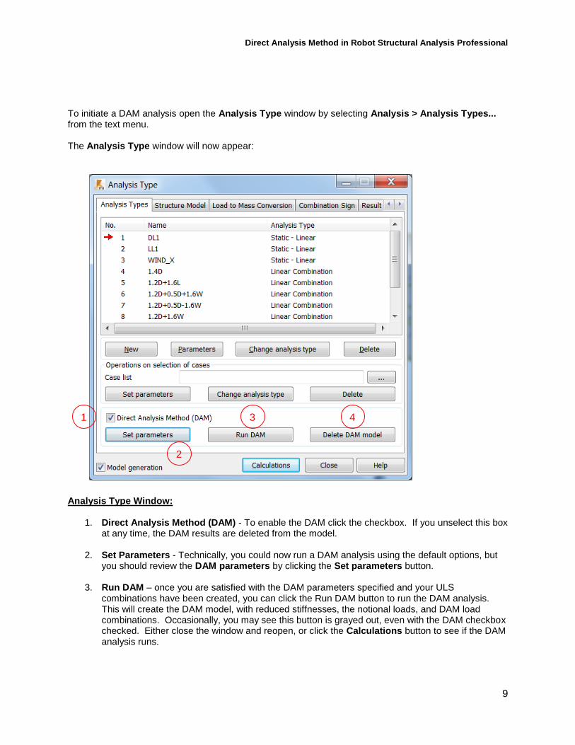
To initiate a DAM analysis open the Analysis Type window by selecting Analysis > Analysis Types... from the text menu. The Analysis Type window will now appear:

Analysis Type Window:

1. Direct Analysis Method (DAM) - To enable the DAM click the checkbox. If you unselect this box at any time, the DAM results are deleted from the model.

2. Set Parameters - Technically, you could now run a DAM analysis using the default options, but you should review the DAM parameters by clicking the Set parameters button.

3. Run DAM – once you are satisfied with the DAM parameters specified and your ULS combinations have been created, you can click the Run DAM button to run the DAM analysis. This will create the DAM model, with reduced stiffnesses, the notional loads, and DAM load combinations. Occasionally, you may see this button is grayed out, even with the DAM checkbox checked. Either close the window and reopen, or click the Calculations button to see if the DAM analysis runs.

1

2

4

1

3


10

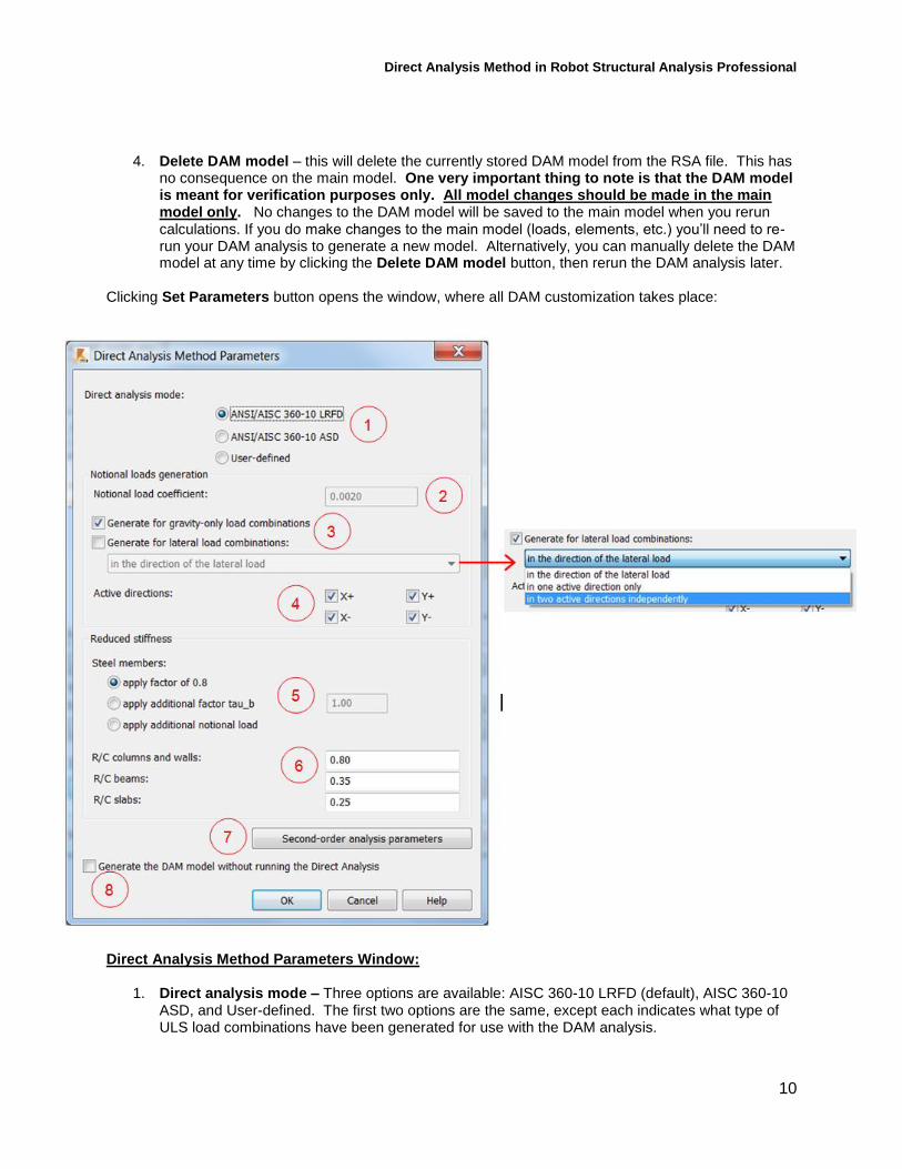
4. Delete DAM model – this will delete the currently stored DAM model from the RSA file. This has no consequence on the main model. One very important thing to note is that the DAM model is meant for verification purposes only. All model changes should be made in the main model only. No changes to the DAM model will be saved to the main model when you rerun calculations. If you do make changes to the main model (loads, elements, etc.) you’ll need to re-run your DAM analysis to generate a new model. Alternatively, you can manually delete the DAM model at any time by clicking the Delete DAM model button, then rerun the DAM analysis later.

Clicking Set Parameters button opens the window, where all DAM customization takes place:

Direct Analysis Method Parameters Window:

1. Direct analysis mode – Three options are available: AISC 360-10 LRFD (default), AISC 360-10 ASD, and User-defined. The first two options are the same, except each indicates what type of ULS load combinations have been generated for use with the DAM analysis.


11

The User-defined option allows for customization of the notional load coefficient and simplifies the steel member stiffness option to a single stiffness reduction which can be specified directly. Notional loads generation:

2. Notional load coefficient – this text box displays the current notional load coefficient for the AISC modes, which will adjust pending decisions made about 𝜏𝑏 below. If User-defined mode is used you can manually set this value.

3. Load combination checkboxes – These two checkboxes allow you to specify which load combinations the generated notional loads will be added to. The top checkbox adds notional loads to gravity-load only combinations, while the second one adds them to the lateral load combinations as well. When you select the generate for lateral load combinations checkbox, you can now select the direction in which the notional loads will act: In the direction of the lateral load – notional loads created will be aligned to the resultant of all lateral loads in each load combination. In one active direction only – notional loads created will act in the closest global axis direction of the resultant of all lateral loads in each load combination. In two active directions independently – notional loads will be created in two independent orthogonal global axis directions, if the sum of the lateral loads in each combination is found to not lie along one of the global axis directions. The notional loads NL1 and NL2 will be in separate load combinations.

4. Active directions – these four checkboxes control which directions notional loads will be generated for. Regardless of how notional loads are specified for lateral load combinations, notional loads will only be created in a direction if the active direction checkbox is selected. Reduced stiffness:

5. Steel Member Stiffness – this section of radio buttons controls the stiffness reduction for steel members for member capacity calculations (only): Apply a factor of 0.8 – reduces stiffness of all steel members by 20%, 𝜏𝑏 = 1.0. Apply additional tau_b factor – selecting this option allows the user to specify a specific value

of 𝜏𝑏. A factor of 0.8 * 𝜏𝑏 will be applied to all steel members stiffnesses in the model. Apply additional notional load – reduces stiffness of all steel members by 20%, 𝜏𝑏 = 1.0, but an

additional notional load of 0.001𝛼𝑌𝑖 is applied to all levels in all load combinations. The direction of the notional load is the same as per the options above. Selecting this will force notional loads to be added to lateral load combinations, so that load combination checkbox will be checked and


12

cannot be unchecked if this option is selected.

6. R/C stiffness reductions – you can select a stiffness reduction factor for reinforced concrete columns and walls, beams, and slabs. By default values, these values should match ACI 318 recommendations for cracked concrete members, but you can select any value you choose.

7. Second-order analysis parameters – this button opens up a new windows where you can specify different parameters used for the second-order analysis. This window is very similar to the non-linear analysis options found in the Structural Analysis section of the Job Preferences window. In fact, there is a Get settings from preferences button, which copies the non-linear analysis parameters for use with the DAM second-order analysis. There are many analysis options here but they are more advanced and beyond the scope of our discussion.

8. Generate the DAM model without running the Direct Analysis – this option is self-explanatory, but could be useful if you want to view the DAM model without the design calculations considering the DAM results.

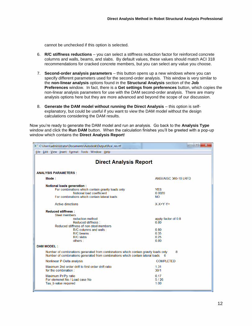
Now you’re ready to generate the DAM model and run an analysis. Go back to the Analysis Type window and click the Run DAM button. When the calculation finishes you’ll be greeted with a pop-up window which contains the Direct Analysis Report!


13

The Direct Analysis Report contains a summary of the DAM parameters specified by the user, but it also contains some very useful information about the DAM model generated including:

1. Number of combinations generated which contain gravity loads only and lateral loads 2. Status of the P-Delta analysis 3. Maximum value of Δ2nd order / Δ1st order and for which combinations it occurs 4. Maximum 𝑃𝑟 𝑃𝑦⁄ ratio and for which element and load case

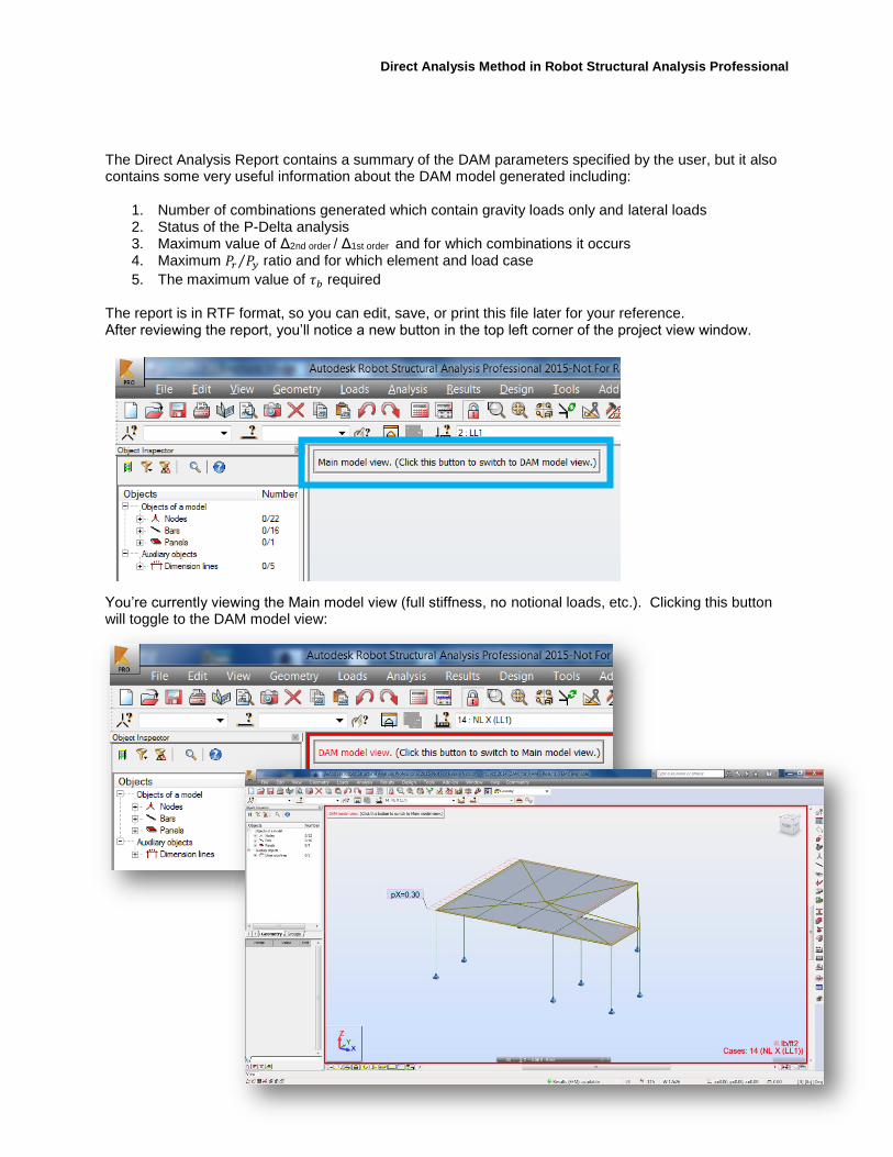
5. The maximum value of 𝜏𝑏 required The report is in RTF format, so you can edit, save, or print this file later for your reference. After reviewing the report, you’ll notice a new button in the top left corner of the project view window.

You’re currently viewing the Main model view (full stiffness, no notional loads, etc.). Clicking this button will toggle to the DAM model view:

5


14

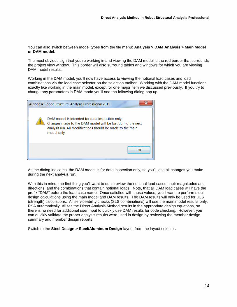
You can also switch between model types from the file menu: Analysis > DAM Analysis > Main Model or DAM model. The most obvious sign that you’re working in and viewing the DAM model is the red border that surrounds the project view window. This border will also surround tables and windows for which you are viewing DAM model results. Working in the DAM model, you’ll now have access to viewing the notional load cases and load combinations via the load case selector on the selection toolbar. Working with the DAM model functions exactly like working in the main model, except for one major item we discussed previously. If you try to change any parameters in DAM mode you’ll see the following dialog pop up:

As the dialog indicates, the DAM model is for data inspection only, so you’ll lose all changes you make during the next analysis run.

With this in mind, the first thing you’ll want to do is review the notional load cases, their magnitudes and directions, and the combinations that contain notional loads. Note, that all DAM load cases will have the prefix “DAM” before the load case name. Once satisfied with these values, you’ll want to perform steel design calculations using the main model and DAM results. The DAM results will only be used for ULS (strength) calculations. All serviceability checks (SLS combinations) will use the main model results only. RSA automatically utilizes the Direct Analysis Method results in the appropriate design equations, so there is no need for additional user input to quickly use DAM results for code checking. However, you can quickly validate the proper analysis results were used in design by reviewing the member design summary and member design reports.

Switch to the Steel Design > Steel/Aluminum Design layout from the layout selector.

6

8 7


15

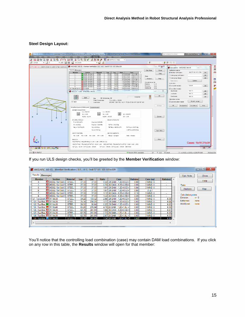
Steel Design Layout:

If you run ULS design checks, you’ll be greeted by the Member Verification window:

You’ll notice that the controlling load combination (case) may contain DAM load combinations. If you click on any row in this table, the Results window will open for that member:


16

You can verify you’re viewing both DAM and Main model results in this window by the naming of the first two tabs (Simplified results (DAM model) and Displacements (Main model)). You’ll also likely see some DAM prefixes on some of the load cases referenced in the first tab.

You can now go about your design checks and revisions as you normally would. The only thing to remember is that you should make your changes to the main model and then update your DAM model results as you iterate your member designs. You can still optimize beam sections, but since the results of the DAM model depend on member stiffnesses, notional loads, etc., you’ll want to update your DAM model when making significant changes. During the presentation we’ll walk through this process.

Current limitations of the DAM in RSA:

1. The DAM currently supports the use of static seismic analysis approaches only, such as the equivalent lateral force procedure. Nonstatic load cases, such as spectral seismic analysis, will not be considered in the DAM model generation, they’ll simply won’t appear in the DAM model but will remain in the Main model.

2. The DAM analysis is currently not compatible with a phased structure. If you have a structure with phasing which you want to use the DAM, you’ll need to save a separate file and remove the phasing for that model.


17

Conclusions

The DAM provides an opportunity for engineers to produce more accurate, safer, and more transparent

designs for any steel framed structure. While conducting a rigorous implementation of the DAM requires

a complex analysis solver and more computing power, RSA’s implementation is very fast and accurate,

with negligible increasing in calculation time. Of course, all of this would be a moot point if the workflow

to implement the DAM is cumbersome. However, as we’ve seen, RSA’s DAM implementation is very

logical and integrates seamlessly into a normal steel design workflow. RSA doesn’t impose

simplifications on the user to make the experience more streamlined, the user is in full control.

direct analysis method in robot structural analysis ... · pdf filedirect analysis method in...

Documents