direct feed flow controlled solar combisystem with non-pressurized
TRANSCRIPT

Direct Feed Flow Controlled Solar
Combisystem with Non-pressurized Storage: a Simulation Case
Martino Poretti
Prof. Aldo Steinfeld Supervisor: P. Vogelsanger
Zürich, 17. February 2006
Diploma Thesis WS 05/06 Institute of Energy Technology, ETHZ Zürich
Solartechnik Prüfung Forschung
Storage Task 32

Diploma Thesis WS 2005/06
Martino Poretti SolartechnikPrüfungForschung
_______________________________________________________________________
1
Martino Poretti Diplomsemester D-MAVT 00-911-206
Via Bonzaglio 14 CH-6997 Sessa Email: [email protected] Tel: +41 78 824 13 53
Diploma Thesis WS 2005/06
Martino Poretti SolartechnikPrüfungForschung
_______________________________________________________________________
2
Table of Contents 1. Abstract .................................................................................... 13
2. Introduction.............................................................................. 14
2.1. Actual Situation.........................................................................................14
2.2. Technology Description ............................................................................15 2.2.1. Drain-back technology ..........................................................................................15 2.2.2. Non-pressurized storage tank ...............................................................................16
3. Goals......................................................................................... 17
4. TRNSYS 16 ............................................................................... 19
5. Direct Feed Flow Controlled System..................................... 20
5.1. Introduction ...............................................................................................20
5.2. TRNSYS Model ........................................................................................20
5.3. Definition of the components included in the system................................21 5.3.1. Collector................................................................................................................21 5.3.2. Pipes between collector and storage ....................................................................22 5.3.3. Storage .................................................................................................................23 5.3.4. Boiler.....................................................................................................................24 5.3.5. Domestic hot water ...............................................................................................26 5.3.6. Building .................................................................................................................28 5.3.7. Heat distribution ....................................................................................................29
5.4. Control strategy ........................................................................................30 5.4.1. Control of the collector loop ..................................................................................30 5.4.2. Control of the auxiliary heater ...............................................................................31 5.4.3. Control of the space heating .................................................................................32
6. The Reference System............................................................ 34
6.1. Introduction ...............................................................................................34

Diploma Thesis WS 2005/06
Martino Poretti SolartechnikPrüfungForschung
_______________________________________________________________________
3
6.2. TRNSYS Model ........................................................................................34
6.3. Definition of the components included in the system................................35 6.3.1. Collector................................................................................................................35 6.3.2. Pipes between Collector and Storage...................................................................35 6.3.3. Storage .................................................................................................................35 6.3.4. Boiler.....................................................................................................................36 6.3.5. Domestic hot water ...............................................................................................37 6.3.6. Building .................................................................................................................37 6.3.7. Heat distribution ....................................................................................................37
6.4. Control strategy ........................................................................................39 6.4.1. Control of the collector loop ..................................................................................39 6.4.2. Control of the auxiliary heater ...............................................................................39 6.4.3. Control of the space heating .................................................................................40
7. Definitions ................................................................................ 42
7.1. Nomenclature ...........................................................................................42
7.2. Target Function.........................................................................................43
8. Validation of the model ........................................................... 44
8.1. Time step ..................................................................................................44
8.2. Convergence and integral tolerances .......................................................44 8.2.1. Direct Deed Flow Controlled .................................................................................44 8.2.2. Reference model...................................................................................................45
8.3. Energy balance.........................................................................................46 8.3.1. Direct Feed Flow Controlled..................................................................................46 8.3.2. Reference model...................................................................................................46
9. Sensitivity analysis and optimization.................................... 47
9.1. Introduction ...............................................................................................47
9.2. Boiler Type 269 analyses .........................................................................47 9.2.1. Steady state ..........................................................................................................47 9.2.2. Unsteady state ......................................................................................................50 9.2.3. Conclusion ............................................................................................................51

Diploma Thesis WS 2005/06
Martino Poretti SolartechnikPrüfungForschung
_______________________________________________________________________
4
9.3. Direct Feed Flow Controlled system parameter analysis..........................52 9.3.1. Introduction ...........................................................................................................52 9.3.2. Auxiliary heater .....................................................................................................52 9.3.3. Storage tank..........................................................................................................60 9.3.4. Collector loop ........................................................................................................63 9.3.5. Domestic hot water ...............................................................................................67 9.3.6. Space heating loop ...............................................................................................70 9.3.7. Conclusions ..........................................................................................................78
9.4. Reference model parameter analysis .......................................................79 9.4.1. Introduction ...........................................................................................................79 9.4.2. Auxiliary heater .....................................................................................................79 9.4.3. Space heating loop ...............................................................................................81 9.4.4. Conclusions ..........................................................................................................87
10. Comparison between the two concepts................................ 88
10.1. Introduction............................................................................................88
10.2. Space heating control management ......................................................88
10.3. Overall system efficiency .......................................................................91
11. Direct Feed versus Heat Exchangers .................................... 94
11.1. Introduction............................................................................................94
11.2. Solar loop heat exchanger.....................................................................97
11.3. Space heating loop heat exchanger ....................................................100
11.4. Solar and space heating loop heat exchangers...................................104
12. Conclusions ........................................................................... 106
13. Acknowledgments................................................................. 107
14. References ............................................................................. 108
14.1. Literature .............................................................................................108
14.2. Internet Links .......................................................................................109

Diploma Thesis WS 2005/06
Martino Poretti SolartechnikPrüfungForschung
_______________________________________________________________________
5
Appendix A - Controller Type 290…………………………………..110 Appendix B - Controller Type 291…………………………………..113 Appendix C – CD files description………………………………….116

Diploma Thesis WS 2005/06
Martino Poretti SolartechnikPrüfungForschung
_______________________________________________________________________
6
List of Tables
Table 5-1: Collector loop data .......................................................................................................... 22 Table 5-2: Collector pipe data .......................................................................................................... 22 Table 5-3: Storage tank data. 1)Relative height: Storage bottom = 0, Storage top = 1 (HE =
heat exchanger) .............................................................................................................. 23 Table 5-4: Boiler data. ...................................................................................................................... 25 Table 5-5: Domestic hot water heat exchanger data....................................................................... 26 Table 5-6: Building data ................................................................................................................... 28 Table 5-7: Floor heating pipe data ................................................................................................... 29 Table 8-1: Influence of the TRNSYS convergence and integral tolerances.................................... 44 Table 8-2: Difference caused by the convergence and the integral tolerances variation............... 44 Table 8-3: Influence of the TRNSYS convergence and integral tolerances.................................... 45 Table 8-4: Difference caused by the convergence and the integral tolerances variation............... 45 Table 8-5: Energy balance of the Direct Feed Flow Controlled System ......................................... 46 Table 8-6: Energy balance of the Reference Model ........................................................................ 46 Table 9-1: Basis case inputs of the boiler stand alone analysis...................................................... 47 Table 9-2: Simulation results as function of the relative height of the storage outlet to the
boiler................................................................................................................................ 54 Table 9-3: Simulation results as function of the minimal modulation range of the gas boiler......... 55 Table 9-4: : Simulation results as function of the boiler mass flow rate for the DHW charging
loop.................................................................................................................................. 56 Table 9-5: Simulation results as function of the C constant ............................................................ 57 Table 9-6: Simulation results as function of the D constant ............................................................ 58 Table 9-7: Simulation results as function of the boiler set supply temperature .............................. 59 Table 9-8: Simulation results as function of the cut off temperature in the storage tank................ 61 Table 9-9: Storage loses coefficient and DHW reserved volume as function of the total
storage tank volume........................................................................................................ 62 Table 9-10: Simulation results as function of the storage tank total volume..................................... 63 Table 9-11: Simulation results as function of the collector area........................................................ 64 Table 9-12: Simulation results as function of the collector a1 coefficient........................................... 65 Table 9-13: Simulation results as function of the collector pump flow rate ....................................... 66 Table 9-14: Simulation results as function of the collector loop storage inlet ................................... 67 Table 9-15: Simulation results as function of the DHW reserved volume........................................ 69 Table 9-16: Simulation results as function of the storage tank set temperature for DHW................ 69

Diploma Thesis WS 2005/06
Martino Poretti SolartechnikPrüfungForschung
_______________________________________________________________________
7
Table 9-17: Simulation results as function of the maximum allowed mass flow rate of the space heating pump .................................................................................................................. 70
Table 9-18: Simulation results as function of the maximum allowed mass flow entering the space heating pump........................................................................................................ 71
Table 9-19 Simulation results as function of the dead band during the SH charging loop.............. 72 Table 9-20: Simulation results as function of the relative position of the sensor 2 (SH) .................. 73 Table 9-21: Simulation results as function of the space heating storage tank outlet........................ 74 Table 9-22: Simulation results as function of the space heating storage tank inlet (without
stratified charging mode) ................................................................................................ 75 Table 9-23: Simulation results as function of the space heating pipe loss coefficient...................... 76 Table 9-24: Simulation results as function of the space heating pipe length .................................... 77 Table 9-25: Simulation results as function of the space heating load............................................... 78 Table 9-26: Simulation results as function of the relative height of the storage tank outlet to the
boiler................................................................................................................................ 80 Table 9-27: Simulation results as function of the boiler mass flow rate during the SH charging
loop.................................................................................................................................. 80 Table 9-28: Simulation results as function of the position of the sensor 2 used by the SH
controller.......................................................................................................................... 81 Table 9-29: Simulation results as function of the relative height of the storage tank outlet to the
space heating.................................................................................................................. 82 Table 9-30: Simulations results as function of the space heating pump flow rate ........................... 83 Table 9-31: Simulation result as function of the SH pump flow rate ................................................. 84 Table 9-32: Simulation results as function of the space heating pipe loss coefficient...................... 85 Table 9-33: Simulation results as function of the space heating pipe length .................................... 86 Table 9-34: Simulation results as function of the space heating load............................................... 87 Table 10-1: Overall system efficiency comparison of the DFFC concept referred to the
reference system. ........................................................................................................... 91 Table 11-1: Solar loop heat exchanger parameters 1)Relative height: Storage bottom = 0,
Storage top = 1 ............................................................................................................... 95 Table 11-2: UA0 coefficient as function of the solar loop heat exchanger area ................................ 95 Table 11-3: Space heating loop heat exchanger parameters 1)Relative height: Storage bottom
= 0, Storage top = 1 ........................................................................................................ 96 Table 11-4: UA0 coefficient as function of the space heating loop heat exchanger area ................. 96 Table 11-5: Simulation results as function of the heat exchanger inlet relative height..................... 98 Table 11-6: Simulation results as function of the sensor 3 relative height........................................ 99 Table 11-7: Simulation results as function of the heat exchanger area .......................................... 100

Diploma Thesis WS 2005/06
Martino Poretti SolartechnikPrüfungForschung
_______________________________________________________________________
8
Table 11-8: Simulation results as function of the space heating heat exchanger tank inlet relative height................................................................................................................ 102
Table 11-9: Simulation results as function of the sensor 2 relative position in storage .................. 103 Table 11-10: Simulation results function of the space heating heat exchanger area ...................... 104 Table 11-11: Simulation results of the system represented by the Figure 11-11............................. 105

Diploma Thesis WS 2005/06
Martino Poretti SolartechnikPrüfungForschung
_______________________________________________________________________
9
List of Figures
Figure 2-1: Standard combisystem example .................................................................................... 14 Figure 2-2: Example of the drain-back technology ........................................................................... 15 Figure 3-1: Direct feed flow controlled combisystem ........................................................................ 17 Figure 5-1: Direct Feed Flow Controlled system diagram ................................................................ 21 Figure 5-2: Storage tank detail .......................................................................................................... 24 Figure 5-3: Boiler loop in detail.......................................................................................................... 25 Figure 5-4: Domestic hot water heat exchanger in detail ................................................................. 26 Figure 5-5: Cold water temperature profile over an year .................................................................. 27 Figure 5-6: Example of draw profile over one week ......................................................................... 27 Figure 5-7: Heat power demand over one year in kW...................................................................... 28 Figure 5-8: Space heating loop in detail............................................................................................ 29 Figure 5-9: Collector loop control system in detail ............................................................................ 31 Figure 5-10: Boiler loop control system in detail ................................................................................. 32 Figure 5-11: Space heating loop control system in detail ................................................................... 33 Figure 6-1: Reference system diagram............................................................................................. 35 Figure 6-2: Storage tank detail .......................................................................................................... 36 Figure 6-3: Boiler loop in detail.......................................................................................................... 37 Figure 6-4: Space heating loop in detail............................................................................................ 38 Figure 6-5: Space heating pump flow rate curve .............................................................................. 38 Figure 6-6: Boiler loop control system in detail ................................................................................. 40 Figure 6-7: Heat power in function of the SH supply temperature ................................................... 41 Figure 9-1: Boiler efficiency vs. feed water temperature .................................................................. 48 Figure 9-2: Boiler efficiency vs. water mass flow rate....................................................................... 48 Figure 9-3: Condensation gain vs. feed water temperature ............................................................. 48 Figure 9-4: Condensation gain vs. water mass flow ......................................................................... 48 Figure 9-5: Boiler efficiency as function of the feed water temperature and the lambda value ....... 49 Figure 9-6: Boiler efficiency as function of the feed water temperature and the combustion air
temperature..................................................................................................................... 49 Figure 9-7: Boiler efficiency as function of the feed water temperature and the set supply
temperature..................................................................................................................... 49 Figure 9-8: Boiler efficiency as function of the feed water temperature and the relative humidity
of the air .......................................................................................................................... 49

Diploma Thesis WS 2005/06
Martino Poretti SolartechnikPrüfungForschung
_______________________________________________________________________
10
Figure 9-9: Boiler efficiency as function of the water feed temperature ........................................... 50 Figure 9-10: Boiler efficiency as function of the boiler mass flow rate ............................................... 51 Figure 9-11: Saving function as function of the relative position of the storage outlet to the boiler... 53 Figure 9-12: Solar fraction and boiler efficiency as function of the relative position of the storage
outlet to the boiler ........................................................................................................... 53 Figure 9-13: Boiler efficiency and condensation gain as function of the relative position of the
storage outlet to the boiler .............................................................................................. 53 Figure 9-14: Saving function as function of the minimal modulation range of the gas boiler............. 54 Figure 9-15: Boiler efficiency and number of boiler starts as function of the minimal modulation
range of the gas boiler .................................................................................................... 54 Figure 9-16: Saving function and boiler efficiency as function of the boiler mass flow rate for the
DHW charging loop......................................................................................................... 55 Figure 9-17: Saving function as function of the C constant ................................................................ 56 Figure 9-18: Boiler efficiency and solar fraction as function of the C constant .................................. 56 Figure 9-19: Saving function as function of the D constant ................................................................ 58 Figure 9-20: Boiler efficiency and solar fraction as function of the D constant .................................. 58 Figure 9-21: Heat energy delivered by the space heating as function of the D constant .................. 58 Figure 9-22: Saving function as function of the boiler set supply temperature .................................. 59 Figure 9-23: Storage loses and boiler efficiency as function of the boiler set supply temperature.... 59 Figure 9-24: Saving function as function of the cut off temperature in the storage tank.................... 60 Figure 9-25: Solar fraction as function of the cut off temperature in the storage tank ....................... 60 Figure 9-26: Collector pipes and storage tank loses as function of the cut off temperature in the
storage ............................................................................................................................ 61 Figure 9-27: Saving function as function of the storage tank total volume......................................... 62 Figure 9-28: Solar fraction as function of the storage tank total volume ............................................ 62 Figure 9-29: Energy difference from the base case as function of the storage tank volume............. 63 Figure 9-30: Saving function as function of the collector area............................................................ 64 Figure 9-31: Solar fraction as function of the collector area ............................................................... 64 Figure 9-32: Saving function as function of the collector a1 coefficient .............................................. 65 Figure 9-33: Solar fraction as function of the collector a1 coefficient.................................................. 65 Figure 9-34: Saving function as function of the collector pump flow rate........................................... 66 Figure 9-35: Solar fraction as function of the collector pump flow rate .............................................. 66 Figure 9-36: Saving function as function of the collector loop storage inlet ....................................... 67 Figure 9-37: Solar fraction and boiler efficiency as function of the collector loop storage inlet ......... 67 Figure 9-38: Saving function as function of the DHW reserved volume............................................ 68

Diploma Thesis WS 2005/06
Martino Poretti SolartechnikPrüfungForschung
_______________________________________________________________________
11
Figure 9-39: Boiler efficiency and solar fraction as function of the DHW reserved volume.............. 68 Figure 9-40: Liters of DHW that don’t match the comfort temperature of 40 °C over a year as
function of the DHW reserved volume............................................................................ 68 Figure 9-41: Saving function as function of the storage tank set temperature for DHW.................... 69 Figure 9-42: Liters of DHW that don’t match the comfort temperature of 40 °C over a year as
function of the storage tank set temperature for DHW................................................... 69 Figure 9-43: Saving function and energy delivered by the space heating as function of the
maximum allowed water temperature entering the space heating loop ........................ 70 Figure 9-44: Saving function as function of the maximum allowed mass flow entering the space
heating pump .................................................................................................................. 71 Figure 9-45: Saving function as function of the dead band during the SH charging loop.................. 72 Figure 9-46: Saving function as function of the relative position of the sensor 2 (SH) ...................... 73 Figure 9-47: Boiler starts as function of the relative position of the sensor 2 (SH) ............................ 73 Figure 9-48: Saving function as function of the space heating storage tank outlet............................ 74 Figure 9-49: Solar fraction and boiler efficiency as function of the space heating storage outlet...... 74 Figure 9-50: Saving function as function of the space heating storage tank inlet.............................. 75 Figure 9-51: Solar fraction and boiler efficiency as function of the space heating storage tank
inlet .................................................................................................................................. 75 Figure 9-52: Saving function as function of the space heating pipe loss coefficient.......................... 76 Figure 9-53: Boiler efficiency and solar fraction as function of the space heating pipe loss
coefficient ........................................................................................................................ 76 Figure 9-54: Saving function as function of the space heating pipe length........................................ 77 Figure 9-55: Boiler efficiency and solar fraction as function of the space heating pipe length .......... 77 Figure 9-56: Saving function as function of the relative height of the storage tank outlet to the
boiler................................................................................................................................ 79 Figure 9-57: Boiler efficiency and solar fraction as function of the relative height of the storage
tank outlet to the boiler.................................................................................................... 79 Figure 9-58: Saving function as function of the boiler mass flow rate during the SH charging
loop.................................................................................................................................. 80 Figure 9-59: Boiler efficiency as function of the boiler mass flow rate during the SH charging
loop.................................................................................................................................. 80 Figure 9-60: Saving function as function of the position of the sensor 2 used by the SH
controller.......................................................................................................................... 81 Figure 9-61: Saving function as functions of the relative height of the storage tank outlet to the
space heating.................................................................................................................. 82 Figure 9-62: Saving function as function of the space heating pump flow rate.................................. 83 Figure 9-63: Boiler efficiency and solar fraction as function of the space heating pump flow rate .... 83 Figure 9-64: Saving function as function of the SH pump flow rate ................................................... 84

Diploma Thesis WS 2005/06
Martino Poretti SolartechnikPrüfungForschung
_______________________________________________________________________
12
Figure 9-65: Boiler efficiency and solar fraction as function of the SH pump flow rate...................... 84 Figure 9-66: Saving function as function of the space heating pipe loss coefficient.......................... 85 Figure 9-67: Solar fraction and boiler efficiency as function of the space heating pipe loss
coefficient ........................................................................................................................ 85 Figure 9-68: Saving function as function of the space heating pipe length........................................ 86 Figure 9-69: Boiler efficiency and solar fraction as function of the space heating pipe length .......... 86 Figure 10-1: Space heating return temperature as function of the heating power and the supply
temperature..................................................................................................................... 88 Figure 10-2: Heating power as function of the supply temperature of the reference system ............ 89 Figure 10-3: Return temperature as function of the supply temperature of the reference system .... 89 Figure 10-4: Heating power and return temperature as function of the supply temperature and
the mass flow rate of the space heating pump............................................................... 90 Figure 10-5: Saving function comparison between the DFFC and reference system as function
of the space heating pipe heat loss coefficient .............................................................. 92 Figure 10-6: Boiler efficiency comparison between the DFFC and reference system as function
of the space heating pipe heat loss coefficient .............................................................. 92 Figure 10-7: Solar fraction comparison between the DFFC and reference system as function of
the space heating pipe heat loss coefficient .................................................................. 92 Figure 10-8: Saving function comparison between the DFFC and reference system as function
of the space heating pipe length..................................................................................... 93 Figure 10-9: Boiler efficiency comparison between the DFFC and reference system as function
of the space heating pipe length..................................................................................... 93 Figure 10-10: Solar fraction comparison between the DFFC and reference system as function of
the space heating pipe length......................................................................................... 93 Figure 11-1: Solar loop heat exchanger capacity rate curves ............................................................ 95 Figure 11-2: Space heating loop heat exchanger capacity rate curves ............................................. 96 Figure 11-3: Storage tank detail .......................................................................................................... 97 Figure 11-4: Saving function as function of the heat exchanger inlet relative height......................... 98 Figure 11-5: Saving function as function of the sensor 3 relative height............................................ 99 Figure 11-6: Saving function as function of the heat exchanger area .............................................. 100 Figure 11-7: Storage tank detail ........................................................................................................ 101 Figure 11-8: Saving function as function of the space heating heat exchanger inlet height............ 102 Figure 11-9: Saving function as function of the sensor 2 relative position in storage...................... 103 Figure 11-10: Saving function as function of the space heating heat exchanger area .................... 104 Figure 11-11: Storage tank detail ...................................................................................................... 105
Figure A-1: Heating pipe detail…………………………………………………………………………….110
Figure A-2: Type 290 black box illustration……………………………………………………………....111

Diploma Thesis WS 2005/06
Martino Poretti SolartechnikPrüfungForschung
_______________________________________________________________________
13
1. Abstract The key design challenge for a solar combisystem is how to integrate the different requirements of the heating source and the heating loads into a single, cost-effective, durable and reliable heating system while achieving the most benefit from each installed square meter of collector.
The assignment of this diploma project was to simulate a new concept of solar combisystem using the program TRNYS 16. This system is characterized by a non-pressurized storage tank and drain back collectors. All the load and unload process performed on the storage tank is done directly, without use of any heat exchanger. In addition, the space heating loop control is uncommon, the heat power is controlled by the space heating pump mass flow rate, and not, as in a traditional system, by varying the space heating supply temperature.
The results of this concentrated simulation effort show that a Direct Feed Flow Controlled combisystem has a good potential of efficiency improvement compared to a standard solar combisystem. Through this special space heating controller the return temperature to the storage can by significantly lowered, thus increasing the solar gain and the boiler efficiency.
The results also show that a storage tank directly fed allows a much higher overall system efficiency if compared to a combisystem storage with integrated heat exchangers.

Diploma Thesis WS 2005/06
Martino Poretti SolartechnikPrüfungForschung
_______________________________________________________________________
14
2. Introduction 2.1. Actual Situation Throughout the world, hundreds of thousands of domestic solar hot water systems are demonstrating the possibilities of this renewable energy source. Due to the success of these hot water systems, more builders are turning to solar energy for space heating. The heating requirements of a single- or multi-family house can be met at acceptable costs by combining solar heating systems with short-term heat storage and well-insulated buildings.
The further development of this solar thermal system is characterized by two key factors that are of major interest for the future development of solar heating systems for household use. These factors are:
• Drain-back system
• Non-pressurized storage tank
The SPF (Solartechnik Prüfung Forschung) institute of Rapperswill is a member of the international program IEA SHC (International Energy Agency for Solar Heating and Cooling) and is responsible for the optimization of hot water storage concepts. Its attention is most of all focused on the load and unload loop of different solar systems in combination of non-pressurized storage tanks. The goal is first of all to achieve a significant cost reduction of the solar combisystem while maintaining maximum system efficiency.
In a combisystem there are at least two energy sources used to supply heat to the two heat consumers (domestic hot water and space heating). The solar collectors deliver heat as long as solar energy is available, and the auxiliary energy source (oil, gas, wood, electricity, etc.) supplements the missing heat required. The key challenge in creating a combisystem is to combine the different requirements of heat suppliers and heat consumers into one single, cost-effective, durable and reliable heating system, achieving the most benefit from each installed square meter of collectors.
Figure 2-1: Standard combisystem example

Diploma Thesis WS 2005/06
Martino Poretti SolartechnikPrüfungForschung
_______________________________________________________________________
15
2.2. Technology Description
2.2.1. Drain-back technology
Drain-back technology provides an interesting alternative for protection against overheating of the fluid in the solar collector loop and also prevents the heat transfer fluid from freezing. The use of a drain-back system allows the operation of the circulation using natural water without antifreeze additives.
The system concept is based on draining the water from the tilted collector and out of the collector pipes using gravitational force, while replacing the liquid with air from the top. Without water in collector and pipes ice cannot form and damage is therefore avoided. The water also drains back if the heat store is fully charged, avoiding boiling of water and high pressure inside pressurized systems.
drainback level
drainback tank
Figure 2-2: Example of the drain-back technology
In comparison with the use of heat transfer fluids (antifreeze) drain-back technology using water features shows both advantages and disadvantages.
+ Heat transfer properties of water (thermal capacity and viscosity) are better than those of other heat transfer fluids.
+ Water is much cheaper than all other collector fluids and easily available

Diploma Thesis WS 2005/06
Martino Poretti SolartechnikPrüfungForschung
_______________________________________________________________________
16
+ The collector loop generally does not face high overpressure
+ Level of maintenance for drain-back systems is lower
- Less flexibility in the choice of the solar collector
- Collector loop design and installation need particular attention
The potential of drain-back technology is high due to excellent thermal properties, inherent safety, low cost and easy maintenance. The major barrier far drain-back technology is a lack of skilled workers needed for proper installation.
2.2.2. Non-pressurized storage tank
In a traditional combisystem the storage tank is under pressure; this implies a much more expensive storage system because good mechanical properties of the materials are required.
A non-pressurized storage tank can instead be made of plastic materials or low quality steels, achieving a reduction in material and manufacturing cost that can be significant. One problem with a polymer made storage tank is the maximal temperature allowed, which could be lower than that of a traditional storage tank under pressure.

Diploma Thesis WS 2005/06
Martino Poretti SolartechnikPrüfungForschung
_______________________________________________________________________
17
3. Goals The goal of this diploma thesis is to check the performance of a Direct Feed Flow Controlled solar combisystem that includes the two technologies described in chapter 2.2 and to compare it to a standard reference combisystem.
Direct Feed Flow Controlled means that the heating power for the space heating is not varied as in a traditional system by changing the supply temperature. Instead, the modulation of the heating power is performed by modulating the flow rate of the water supply entering the space heating loop. This feature yields, in an optimum case, a much lower return temperature to the storage tank, which results in theoretical benefits such as higher solar efficiency and better water condensation in a gas boiler. This supposition should be confirmed by the simulation.
a.
b. d.
e.
c.
a. Collector b. Storage tank c. Space heating d. Auxiliary heater e. Domestic hot water
Figure 3-1: Direct feed flow controlled combisystem
The system is schematically represented in Figure 3-1. The drain-back collector-loop (a.) is directly connected to a non-pressurized storage tank (without the use of any heat exchanger) and the auxiliary heater (d.) is directly coupled to the storage tank. Compared to common solar systems this is uncommon. The auxiliary heater runs at a constant temperature to keep a determined temperature at the top of the tank, the zone reserved for domestic hot water. The power adjustment for space heating (c.) is obtained by variation of the mass flow of the space heating pump; this is also uncommon.
A reference model, characterized by a traditional space heating controller must also be modeled.
The systems are simulated using the program TRNSYS 16; the model should be written in a clear manner and documented so as to provide the basis for further developments.
Diploma Thesis WS 2005/06
Martino Poretti SolartechnikPrüfungForschung
_______________________________________________________________________
18
The task to achieve can be summarized in the following points:
• Research of existing simulation models and methods to simulate the auxiliary heater: possibly a gas heater with condensing technology.
• Definition of the Direct Feed Controlled System concept to be investigated and a reference model to allow direct comparisons between the two systems.
• Parameter studies for the two different concepts and optimization of both.
• Comparison of the simulation results relative to the overall system efficiency.
Diploma Thesis WS 2005/06
Martino Poretti SolartechnikPrüfungForschung
_______________________________________________________________________
19
4. TRNSYS 16 To simulate the to different variants of the solar combisystem is used the simulation program TRNSYS version 16.
TRNSYS 16 is a transient systems simulation program with a modular structure. TRNSYS library includes many of the components commonly found in thermal and electrical energy systems, as well as component routines to handle input of weather data or other time-dependent forcing functions and output of simulation results.
The modular nature of TRNSYS gives the program tremendous flexibility, and facilitates the addition to the program of mathematical models not included in the standard TRNSYS library. TRNSYS is well suited to detailed analyses of any system whose behavior is dependent on the passage of time. Main applications include: solar systems (solar thermal and photovoltaic systems), low energy buildings and HVAC systems, renewable energy systems, cogeneration, fuel cells.

Diploma Thesis WS 2005/06
Martino Poretti SolartechnikPrüfungForschung
_______________________________________________________________________
20
5. Direct Feed Flow Controlled System 5.1. Introduction In this chapter is presented the TRNSYS model, with its components and the control strategies used to simulate the Direct Feed Flow Controlled solar combisystem.
5.2. TRNSYS Model Some parts of the TRNSYS model are directly taken from the Solar Reference System v.17 developed by Richard Heimrath within the framework of the IEA Solar Heating and Cooling international program. These components are: the weather processor and weather data, the solar collector module and the domestic hot water heat exchanger. From Heimrath’s Solar Reference System are also generated the load file for the space heating using the weather data of Zürich, since in the this simulation is not present any building model. Unfortunately there isn’t any written documentation concerning the v.17 of the reference system model used in the IEA task.
The choice to eliminate the building model type 56 is made because of two reasons, first to have a very fast simulation so to make possible a wide parameter study and optimization. The second reason is to have exactly the same amount of heat energy delivered by the space heating in each simulation so to make possible a fair comparison between all the results.
The Direct Feed Flow Controlled system represent a drain-back solar combisystem with a non-pressurized storage tank. What makes this concept uncommon is the space heating control philosophy. In this concept the heating power is varied by changing the flow rate of the water supply and not the supply temperature as in traditional systems.
Figure 5-1 shows an overall view of the system model, each component is described in greater detail in the next section.

Diploma Thesis WS 2005/06
Martino Poretti SolartechnikPrüfungForschung
_______________________________________________________________________
21
Figure 5-1: Direct Feed Flow Controlled system diagram
5.3. Definition of the components included in the system In following subsections are described the components and their parameters chosen as „base case“ for the Direct Feed Flow Controlled simulation model.
5.3.1. Collector
The collector is modeled with the non-standard TRNSYS Type 232. The parameter are chosen to match a standard flat plate collector and are described in Table 5-1. The collector pipe are directly connected to the storage tank (without use of any heat exchanger).
The collector loop is a low flow system with a specific mass flow rate through the collectors of 12 l/(m2.h). The overall collector area is 12 m2. The drain-back system is not simulated because it has no influence on the solar gain and on the simulation results, but has to be considered during practical planning and assembly of the solar loop.
Type 109 Weather Data
Type 232 Solar Collector
Type 3 Pump
Type 3 Pump
Type 110 Pump
Type 298 Heat
exchanger
Type 31 Pipe floor space
heating
Type 31 Pipe
Type 31 Pipe
Type 269 Auxiliary
heater
Type 140 Storage
Type 9 Water Draw
Type 9 Heat load
Type 2 Pump Controller
Type 2 Auxiliary heater
controller
Type 11b Temperature limiting valve
Type 290 Heat pump controller

Diploma Thesis WS 2005/06
Martino Poretti SolartechnikPrüfungForschung
_______________________________________________________________________
22
Table 5-1: Collector loop data
Collector a0 0.8 a1 3.5 W/m2.K a2 0.015 W/m2.K Area 12 m2 Tilt angle 45 ° Specific mass flow 12 Kg/m2.h Inc. Angle Modifier 0.9 [-] Effective heat capacity 7000 [J/m2K] Heat transfer media Water
5.3.2. Pipes between collector and storage
The pipes in the collector loop are modeled with a standard TRNSYS Type 31. The geometry and the insulation thickness of the pipes connecting the collectors and the storage tank are given in Table 5-2. For the heat loss calculations, a surrounding temperature of 15°C is given.
The pipes are made of copper (28x1.5) with a 25 mm insulation. A standard length of 15 meters have been chosen for both pipes.
In Equation 5-1 and Equation 5-2 is showed how the pipe U-coefficient is calculated. The resulting U-value is 10.65 W/m2.K
( )isoaa
i
i
isoa
iso
i
i
a
pipe
i
dDD
DdDD
DDD
C⋅+⋅
+⎟⎟⎠
⎞⎜⎜⎝
⎛ ⋅+⋅+⎟⎟
⎠
⎞⎜⎜⎝
⎛⋅=
22
ln2
ln2 αλλ
Equation 5-1
( ) =⋅⋅+
= 6.31 C
Ui
ipipe α
α10.65 [W/m2.K]
Equation 5-2
Table 5-2: Collector pipe data
Collector pipes Length, tank to collector (cold side) 15 m Length, tank to collector (hot side) 15 m Inner diameter (Di) 0.025 m Outer diameter (Da) 0.028 m Insulation thickness (diso) 0.025 m Insulation thermal conductivity (λiso) 0.042 W/m.K Pipe thermal conductivity (λpipe) 372.0 W/m.K Lambda internal (αi) 1000 W/m2.K Lambda external (αa) 10 W/m2.K U-value pipe (Upipe) 10.65 W/m2.K Heat transfer media Water

Diploma Thesis WS 2005/06
Martino Poretti SolartechnikPrüfungForschung
_______________________________________________________________________
23
5.3.3. Storage
The storage tank is modeled with a non-standard TRNSYS Type 140 (version 1.99). This multiport store model is chosen because of the need of an high number of inlet and outlet ports, this possibility wasn’t offered by the standard storage models contained in the TRNSYS libraries.
The storage tank has a volume of 800 liters. As basis values for the thermal heat losses are chosen these of the IEA Reference System, but modified to match a storage volume of 800 liters. The overall heat loss coefficient is 18.08 kJ/h.
The height of the storage is 1.965 m and the diameter is 0.72 m. The insulation thickness is set to 0.15 m for all the storage. At the top of the storage a volume of 240 liters is reserved to the domestic hot water.
The storage tank includes four inlet and four outlet ports, these are reserved for the collector loop, the space heating loop, the auxiliary heater loop and for the domestic hot water heat exchanger loop. Only the solar inlet and the space heating inlet port are stratified-charged, all the others have a fix inlet and outlet height.
The main parameters of the storage tank are summarized in Table 5-3. Figure 5-2 shows the storage system in detail.
Table 5-3: Storage tank data. 1)Relative height: Storage bottom = 0, Storage top = 1 (HE = heat exchanger)
Storage tank Total volume 0.8 m3 Height 1.965 m Diameter 0.72 m Heat loss coefficient 18.08 kJ/h Thermal conductivity of insulation material 0.032 W/m.K Insulation material thickness 0.15 m Vertical thermal conductivity 2.0 W/m.K Solar inlet (stratified-charged) 1) 0.0 - 0.8 Solar outlet 1) 0.0 Auxiliary heater inlet 1) 1.0 Auxiliary heater outlet 1) 0.4 Space heating outlet 1) 0.6 Space heating inlet (stratified-charged) 1) 0.0 – 0.6 Domestic hot water outlet to HE 1) 1.0 Cold water inlet form HE 1) 0.0 Position of sensor 1: DHW storage temperature 1) 0.7 Position of sensor 2: SH storage temperature 1) 0.55 Position of sensor 3: Collector control temp. 1) 0.0 Position of sensor 4: Storage max temp. protection 1) 1.0

Diploma Thesis WS 2005/06
Martino Poretti SolartechnikPrüfungForschung
_______________________________________________________________________
24
Figure 5-2: Storage tank detail
5.3.4. Boiler
The choice of the boiler model was the most difficult to take. It was first tried to implement in the simulation the TRNSYS non-standard Type 170 [6] but because of the lack in good documentation and the impossibility to understand exactly how this model worked under certain conditions it was decided to use the new non-standard Type 269 (version 1.13) [7] recently developed by Michel Haller of the SPF institute. This new TRNSYS module is not yet used in any simulation so it is tested alone to understand how it behaves in different conditions (analysis performed in section 9.2)
TRNSYS non-standard Type 269 is a carbon-based fuels auxiliary heater with condensing technology that allows power modulation. In this case the fuel used is gas. The boiler has a nominal power of 12 kW and modulates in the range of 30%-100%. The chosen parameters are them of the Hoval TopGas® 12 [9] matched to fit the experimental measured values.
When the boiler operates to heat up domestic hot water in the storage tank or to heat the space heating water reserve, the set supply temperature is fixed at 65°C. Hot water enters always at the fixed relative height of 1.0 (the top of the storage tank).
The water mass flow rate of the auxiliary gas heater is instead variable: when the boiler is charging the DHW it’s value is fixed at 200 kg/h but when it charges the storage tank space
DHW 240 liters
Sensor 1: DHW (rel. height 0.7)
Space heating outlet (rel. height 0.6)
Space heating stratified intlet (rel. height 0.0 - 0.6)
Sensor 2: Space heating (rel. height 0.55)
Collector outlet (rel. height 0.0)
Collector stratified inlet (rel. height 0.0 - 0.8)
DHW heat exchanger inlet (rel. height 0.0)
DHW heat exchanger outlet (rel. height 1.0)
Auxiliary heater inlet (rel. height 1.0)
Auxiliary heater outlet (rel. height 0.4)
Sensor 3: Bottom storage temperature (rel. height 0.0)
Sensor 4: Storage protection (rel. height 1.0)

Diploma Thesis WS 2005/06
Martino Poretti SolartechnikPrüfungForschung
_______________________________________________________________________
25
heating zone the mass flow varies depending on the space heating pump flow rate (for a detailed description see 5.4.2: Control of the auxiliary heater).
For the heat loss calculations a surrounding temperature of 15°C is used. The combustion air temperature is also set to 15°C. The auxiliary heater data are summarized in Table 5-4. Figure 5-3 shows the auxiliary loop in detail.
Table 5-4: Boiler data.
Boiler Nominal Power 12 kW Minimal Power (30%) 3.5 kW Set supply temperature (DHW and SH) 65 °C Hysteresis for Tset 5 °C Fuel type Natural gas Ambient temperature in the boiler house 15 °C Air surplus number (λ) 1.2 Modulation range 30%-100% Thermal mass of empty boiler 17.6 kJ/K Volume of water in the boiler 1.5 dm3 Boiler-environment heat transfer coeff. 4.3 kJ/h.K Gas-water heat transfer 110 kJ/h.K Water supply mass flow rate (DHW) 200 kg/h Water supply mass flow rate (SH) variable Air temperature 15°C Relative humidity 0.5 Pressure 1.01325 bar
Figure 5-3: Boiler loop in detail
Type 140
Aux. heater inlet (rel. height 1.0) Type 2
Auxiliary Heater Controller
Aux. heater outlet (rel. height 0.4)
Sensor 1: DHW temp. (rel. height 0.7)
Sensor 2 : Space heating (rel. height 0.55)
Type 269 Auxiliary
Heater
Type 110 Pump

Diploma Thesis WS 2005/06
Martino Poretti SolartechnikPrüfungForschung
_______________________________________________________________________
26
5.3.5. Domestic hot water
The domestic hot water preparation is simulated using the non-standard heat exchanger TRNSYS Type 298. This module acts like a external DHW heat exchanger but without taking into account the heat losses to the environment.
The heat exchanger primary side (hot side) is connected to a double port of the TRNSYS Type 140. The storage tank inlet for the water coming from the heat exchanger is located at a relative height of 0.0 and the outlet at 1.0 as Figure 5-4 illustrates.
The secondary side of the heat exchanger (cold side) is the draw profile of the domestic hot water. This profile was created using the tool for the generation of domestic hot water profiles programmed by Ulrike Jordan [12].
The text file generated contains a list of flow rate values for each time step. The total mean draw-off volume was set to 200 l/day, which represent the daily hot water need of a single family house.
Table 5-5: Domestic hot water heat exchanger data
DHW Heat Exchanger HX heat transfer capacity 10800 [kJ/h.K] Maximum flux primary side 1065 [kg/h]
Figure 5-4: Domestic hot water heat exchanger in detail
DHW 240 liters
DHW heat exchanger inlet (rel. height 0.0)
DHW heat exchanger outlet (rel. height 1.0)
Type 140 Draw-off
TimeTCold Water
Time
Primary Side
Secondary Side

Diploma Thesis WS 2005/06
Martino Poretti SolartechnikPrüfungForschung
_______________________________________________________________________
27
The mass flow rate of the primary side is varied so to have the set temperature of 45°C on the secondary side heat exchanger outlet. This mass flow can vary from 0 to a maximum of 1065 kg/h. The heat transfer capacity of the heat exchanger as a fix value of 10800 kJ/h.K.
The temperature at the secondary side inlet (cold water temperature) is determined by a sinus function that takes into account the temperature oscillations during the year as Figure 5-5 shows. The curve is plotted from the function described by Equation 5-4.
( )( )⎟⎟⎠
⎞⎜⎜⎝
⎛ ⋅−+⋅⋅+=
87602475.273
360sin ShiftShiftAverageColdWater
DtTTT Equation 5-3
AverageT = 9.7 °C
ShiftT = 6.3 °C
ShiftD = 60 days
( )( )8760/5130360sin3.67.9 +⋅⋅+= tTColdWater Equation 5-4
Cold Water Temperature
0.02.04.06.08.0
10.012.014.016.018.0
0 2000 4000 6000 8000Time [Hours]
Tem
pera
ture
[°C
]
Figure 5-5: Cold water temperature profile over an year
Hot Domestic Water Draw Profile for 1 Week
0
200
400
600
800
1000
1200
Flow
rate
[l/h
r]
Figure 5-6: Example of draw profile over one week

Diploma Thesis WS 2005/06
Martino Poretti SolartechnikPrüfungForschung
_______________________________________________________________________
28
5.3.6. Building
The building is not simulated directly into the system. The heat load demand of the building is contained in an external file. This file was generated from the Solar Reference System v. 17 made by R. Heimrat. In the file is contained the temperature inside the building and the heat power needed for each time step to maintain a constant temperature inside the building (this temperature is practically constant during all the heating season at about 20 °C).
The basis case heat load file was generated from an house model with a specific yearly space heat demand for Zürich climate amounting to 60 kWh/m2.a. The building model parameters used in the Solar Reference System developed by R. Heimrat are described in Table 5-6.
Table 5-6: Building data
Building Specific space heating demand for Zürich climate 60 kWh/m2 per year Area 70 m2 Total window area 23 m2 Window U-value 1.4 Window g-value 0.622 External walls, U-value 0.283 W/m2.K Roof, U-value 0.283 W/m2.K Ground floor, U-value 0.283 W/m2.K Mean power (during heat season) 1.5 kW Maximum power 4.3 kW Total space heat needed per year 8379 kWh
Figure 5-7 shows the heat power contained into the heat load file plotted over a year.
Heating Power [single family house 60 kWh/m2.y]
0.00
0.50
1.00
1.50
2.00
2.50
3.00
3.50
4.00
4.50
1 731 1461 2191 2921 3651 4381 5111 5841 6571 7301 8031 8761
Time [Hours]
Pow
er [k
W]
Figure 5-7: Heat power demand over one year in kW

Diploma Thesis WS 2005/06
Martino Poretti SolartechnikPrüfungForschung
_______________________________________________________________________
29
5.3.7. Heat distribution
The heat distribution of the space heating loop is represented by a pipe (TRNSYS standard Type 31), simulating a floor space heating system. The temperature of the environment in which the pipe is located (the room temperature) is given by the building load file but it is practically constant during the heating season (about 20 °C). The water used for the space heating loop is directly taken from the storage tank without the use of any heat exchanger.
Table 5-7: Floor heating pipe data
Space Heating Pipe Pipe length 100 m Pipe diameter 0.025 m Loses coefficient 25 W/m2.K Maximum flow rate 400 kg/h
A Tee-piece and a temperature limiting valve are installed to limit the temperature that goes into the heating pipe to a set value of 55 °C. Below this value the water is directly taken out of the storage and goes into the space heating loop. If the temperature in the storage goes upper the set temperature of 55 °C, the temperature limiting valve mixes the water returning to the storage form the space heating loop with that coming out of the storage to mach the set maximum temperature of 55 °C. The maximum flow rate of the space heating pump is set to 400 kg/h. Figure 5-8 illustrates the space heating loop in detail.
Figure 5-8: Space heating loop in detail
Type 140 Type 31
Pipe floor space heating
Type 11h Tee-piece
Type 11b Temperature limiting valve
Type 110 Pump
Space heating outlet (rel. height 0.6)
Space heating inlet (rel. height 0.0 - 0.6)
Type 290 Space pump
controller

Diploma Thesis WS 2005/06
Martino Poretti SolartechnikPrüfungForschung
_______________________________________________________________________
30
5.4. Control strategy There are three main controllers that control the system. One controls the collector loop pump. Another controls the auxiliary heater and the last one controls the space heating pump.
The collector loop pump and the auxiliary heater controllers are modeled with TRNSYS standard Type 2 controllers. For the space heating a special non-standard TRNSYS Type 290 has been written.
5.4.1. Control of the collector loop
The control strategy of the collector loop has three main functions, in brief:
1. If the water from the collector Tcoll (sensor 5) is at least 11°C warmer than that of the bottom of the storage Tstore,b (sensor 3) the pump is activated. The pump stops working when this temperature difference is lower than 2 °C
2. If the water supply of the collector is above 100°C (Tcoll,max) the pump shuts down.
3. If the store reaches 95°C Tstore,max (sensor 4) the flow of the collector loop pump is stopped.
The control is managed by comparing the following 4 temperatures:
Tcoll : Collector supply temperature (sensor 5) [°C]
Tcoll,max : Maximum supply collector temperature [°C]
Tstore,b : Temperature at the bottom of the storage (sensor 3) [°C]
Tstore,t : Temperature at the top of the storage (sensor 4) [°C]
Tstore,max : Maximum temperature of storage tank [°C]
Figure 5-9 shows how the collector loop is controlled.

Diploma Thesis WS 2005/06
Martino Poretti SolartechnikPrüfungForschung
_______________________________________________________________________
31
Figure 5-9: Collector loop control system in detail
5.4.2. Control of the auxiliary heater
The auxiliary heater always supplies hot water at the set temperature of 65°C (TsetAUX). The auxiliary heater is controlled after the following principles:
1. When the temperature of the DHW; Tstore DHW (measured by the sensor 1 Figure 5-10) gets below the set temperature of 54°C (Tstore,set) auxiliary heat will be supplied to the storage at a flow rate of 200 kg/h ( AUXm& ) until the water reaches the set temperature of 60°C.
2. If the water temperature below the storage tank outlet that goes to the space heating (sensor 2 Figure 5-10) gets below the minimum temperature needed to match the heat demand of the building plus a reserve factor of 2°C (Theat,min+ 2°C) the auxiliary heater is started. In this case the flow rate for the auxiliary heater ( AUXm& ) depends on the supply mass flow rate of the space heating loop ( SHm& ) and follows this simple relation:
AUXm& = SHm& + 30 kg/h.
The addition of 30 kg/h was necessary to avoid very low mass flow rate of the boiler, causing too many on-off cycles of the auxiliary heater. The auxiliary heater shuts down when the temperature TstoreSH gets 5°C higher than the minimum temperature needed to match the heat demand of the house Theat,min.
Following temperature are used to control the auxiliary system:
TsetAUX : Set supply temperature of the auxiliary heater for both DHW and SH.
Type 140
Tcoll (Sensor 5)
Type 2 Solar Pump Controller
Tstore,b (Sensor 3) Tstore,max ; Tcoll,max
Tstore,t (Sensor 4)

Diploma Thesis WS 2005/06
Martino Poretti SolartechnikPrüfungForschung
_______________________________________________________________________
32
Tstore DHW : Store temperature measured by sensor 1, Figure 5-10 [°C]
Tstore SH : Store temperature measured by sensor 2, Figure 5-10 [°C]
Tstore,set : Set temperature of store for the DHW [°C]
Theat,min : Minimum temperature needed at the space heating tank outlet to match the needed heating power contained in the heat load file (measured by sensor 2, Figure 5-10) [°C]
SHm& : Mass flow rate of the space heating loop [kg/h]
AUXm& : Mass flow rate of the auxiliary heater [kg/h]
Figure 5-10: Boiler loop control system in detail
5.4.3. Control of the space heating
In the Direct Feed Flow Controlled system the heating power is not varied by changing the inlet temperature of the supply water as in traditional systems but changing the pump flow rate. A special controller, TRNSYS Non-standard Type 290, is written and compiled to control the pump and achieve this goal.
The power needed at each time step is contained in an external load file as described in section 5.3.6. The space heat controller 290; using as input the room temperature inside the building Troom, the heat power needed Pneeded at each time step and the temperature entering the space heating pipe (Tpipe,SH); chooses the adequate flow rate of the space heating pump to match the needed heating power.
Type 140
Type 2 Auxiliary Heater
Controller
Tstore DHW (sensor 1)
Tstore SH (sensor 2) Type 269 Auxiliary
Heater
AUXm& Tstore,set Theat,min
SHm&

Diploma Thesis WS 2005/06
Martino Poretti SolartechnikPrüfungForschung
_______________________________________________________________________
33
If the temperature at the storage tank outlet (Ttank,SH) is higher than 55°C the tempering valve mixes the storage tank water with the return temperature to have a space heating supply temperature (Tpipe,SH) of 55°C. Other parameter that the controller takes into account for calculation of the flow rate are the heating pipe’s length lpipe its diameter dpipe and the pipe loss coefficient Kpipe.
A more detailed mathematical description of this special controller is presented in appendix A.
Following temperature are used to control the space heating system:
Troom : Room temperature inside the house [°C]
Pneeded : Needed heating power at each timestep [°kW]
Tstorage,SH : Storage temperature at the space heating outlet port [°C]
Tpipe,SH : Water temperature entering the space heating pipe [°C]
TSH,max : Maximum temperature allowed to enter the space heating pipe [°C]
mSH : Mass flow of the space heating pump [kg/h]
lpipe : Length of the space heating pipe [m]
dpipe : Diameter of the space heating pipe [m]
Kpipe : Space heating pipe loses coefficient [W/m2.K]
Figure 5-11: Space heating loop control system in detail
Type 140
Type 290 Space pump
controller
Troom Pneeded
Tstorage,SH
lpipe , dpipe , Kpipe mSH
TSH,max
Tpipe,SH

Diploma Thesis WS 2005/06
Martino Poretti SolartechnikPrüfungForschung
_______________________________________________________________________
34
6. The Reference System 6.1. Introduction A reference model is also modeled in TRNSYS to allow a comparison between the Direct Feed Flow Controlled solar combisystem concept described in chapter 5 and a solar combisystem with a standard space heating control management. In this chapter are described the TRNSYS model, the components used in the simulation and the control strategies of the “base case” of the reference system.
6.2. TRNSYS Model This reference system model represents also a drain-back solar combisystem with direct feed, therefore also in this case there are no heat exchanger in the storage tank. The big difference between this model and the Direct Feed Flow Controlled concept is within the space heat management philosophy. In this case the power of the space heating system is controlled by changing the supply water temperature entering the heating pipes by means of a tempering valve and not varying the mass flow rate of the space heating pump. This control strategy characterize almost all the traditional heating systems.
To make a fair comparison the collector loop, the storage tank and the auxiliary heater parameters as all the load files and weather files are the same as for the Direct Feed Flow Controlled concept. The only changes introduced are in the space heating management and in the storage tank auxiliary heater charging concept that was also adapted to match a traditional charging strategy. Both modification are described in greater detail in the following sections.

Diploma Thesis WS 2005/06
Martino Poretti SolartechnikPrüfungForschung
_______________________________________________________________________
35
Figure 6-1: Reference system diagram
6.3. Definition of the components included in the system In the following subsections are described the components and their parameters chosen as „base case“ for the reference system.
6.3.1. Collector
The collector is exactly the same as that used for the Direct Feed Flow Controlled system described in section 5.3.1.
6.3.2. Pipes between Collector and Storage
The pipes are the same as them of the Direct Feed Flow Controlled system of section 5.3.2.
6.3.3. Storage
The main storage tank parameters are the same as them employed in the Direct Feed Flow Controlled system. In this case there are two separate storage inlet ports for the auxiliary heater supply. The first at the top of the tank (at a relative height of 1.0) used for the domestic hot water charging loop and a second one at a relative height of 0.55 for the space heating
Type 109 Weather Data
Type 232 Solar Collector
Type 3 Pump
Type 3 Pump
Type 110 Pump Type 298
Heat exchanger
Type 31 Pipe floor space
heating
Type 31 Pipe
Type 31 Pipe
Type 269 Auxiliary
heater
Type 140 Storage
Type 9 Water Draw
Type 9 Heat load
Type 291 Tempering Valve
controller
Type 11b Tempering Valve
Type 2 Pump Controller
Type 2 Auxiliary heater
controller

Diploma Thesis WS 2005/06
Martino Poretti SolartechnikPrüfungForschung
_______________________________________________________________________
36
charging loop. It was decided to introduce this modification because almost all the conventional combisystem operate in a similar way.
The position of the temperature sensor for the space heating water (sensor 2 Figure 6-2 ) has been moved and it’s now at a relative height of 0.6; the same height as the space heating outlet.
Figure 6-2: Storage tank detail
6.3.4. Boiler
The boiler model parameters are the same as them used for the Direct Feed Flow Controlled system. As said before in this case there are two different charging loops, the first for the domestic hot water and the second for the space heating. This is a very common characteristic of the standard combisystem configuration. A mixing valve switches to the fist or the second charging port depending on the signals coming from sensor 1 and sensor 2. Figure 6-3 illustrates schematically how the auxiliary heater operates.
DHW 240 liters
Sensor 1: DHW (rel. height 0.7)
Space heating outlet (rel. height 0.6)
Space heating stratified intlet (rel. height 0.0 - 0.6)
Sensor 2: Space heating (rel. height 0.6)
Collector outlet (rel. height 0.0)
Collector stratified inlet (rel. height 0.0 - 0.8)
DHW heat exchanger inlet (rel. height 0.0)
DHW heat exchanger outlet (rel. height 1.0)
Auxiliary heater inlet (DHW) (rel. height 1.0)
Auxiliary heater outlet (DHW and Space Heating (rel. height 0.4)
Sensor 3: bottom tank temperature (rel. Height 0.0)
Auxiliary heater inlet (Space Heating) (rel. height 0.55)

Diploma Thesis WS 2005/06
Martino Poretti SolartechnikPrüfungForschung
_______________________________________________________________________
37
Figure 6-3: Boiler loop in detail
6.3.5. Domestic hot water
Same as that for the Direct Feed Flow Controlled system
6.3.6. Building
The building heat load demand file is the same as that for the Direct Feed Flow Controlled system.
6.3.7. Heat distribution
As for the system of chapter 5.3.7 the space heating element is modeled as a pipe (TRNSYS Type 31). The pipe simulates a floor space heating system. The parameters are maintained the same as them of the Direct Feed Flow Controlled concept. Also in the reference system the water used for the space heating loop is directly taken from the storage without use of any heat exchanger.
Type 140
Type 2 Auxiliary Heater
Controller
DHW and space heating aux. heater outlet (rel. height 0.4)
Sensor 1: DHW (rel. height 0.7)
Sensor 2 : Space heating (rel. height 0.6)
Type 269 Auxiliary
Heater
Space heating aux. heater inlet (rel. height 0.55)
DHW Aux. heater inlet (rel. height 1.0)

Diploma Thesis WS 2005/06
Martino Poretti SolartechnikPrüfungForschung
_______________________________________________________________________
38
Figure 6-4: Space heating loop in detail
As Figure 6-4 illustrates a Tee-piece and a tempering valve are installed to make possible the choice of a set temperature of the water entering the heating pipes.
The space heating loop pump flow rate in the reference system is much higher than that of the Direct Feed Flow Controlled system, which is limited to 400 kg/h. Higher values are common for traditional systems. In the reference system for water supplies higher than 35°C the pump flow rate has a constant value of 1000 Kg/h, for a lower temperature water supply demand the pump flow rate is reduced linearly. This is done because of convergence problems within TRNSYS Type 11b (tempering valve), that occur when the set supply temperature is near to the room temperature.
Pump Flow rate
0
200
400
600
800
1000
1200
20 25 30 35 40 45 50 55 60 65 70 75
Supply temperature [°C]
Pum
p flo
w ra
te [k
g/h]
Figure 6-5: Space heating pump flow rate curve
Type 140 Type 31
Pipe floor space heating
Type 11h Tee-piece
Type 11b Tempering Valve
Type 110 Pump
Space heating outlet (rel. height 0.6)
Space heating inlet (rel. height 0.0 - 0.6)
Type 291 Tempering valve
controller

Diploma Thesis WS 2005/06
Martino Poretti SolartechnikPrüfungForschung
_______________________________________________________________________
39
6.4. Control strategy As for the Direct Feed Flow Controlled model also in the reference system there are three main controllers that control the system. The collector loop pump controller is exactly the same as for the Direct Feed Flow Controlled system. The controller used for the auxiliary heater is modified to allow the charging strategy operated using two storage ports. The space heating controller is totally different from that of the Direct Feed Flow Controlled system. A detailed description of the controllers follows in the next sections.
6.4.1. Control of the collector loop
Same as for the Direct Feed Flow Controlled concept of section 5.4.1
6.4.2. Control of the auxiliary heater
The auxiliary heater is controlled after the following principles:
1. When the temperature of the DHW (Tstore DHW) measured by the sensor 1 (Figure 6-6) gets below the set temperature of 54°C (Tstore,set) auxiliary heat will be supplied to the top storage inlet (relative height of 1.0) at a flow rate of 200 kg/h ( DHWAUXm ,& ) until the water reaches the set temperature of 60°C. The auxiliary heater supply temperature has in this case a constant value of 65°C (TsetAUX,DHW)
2. If the temperature near the storage tank outlet to the space heating, measured by sensor 2 (Figure 6-6), gets below the minimum temperature needed to match the heat demand of the house plus a reserve factor of 2°C (Theat,min+ 2°C); the auxiliary heater is started and hot water is supplied in the second storage tank inlet at a relative height 0.55. The auxiliary heater shuts down when the temperature of the sensor 2 is 7°C higher than Theat,min. During the space heating charging loop the supply temperature of the auxiliary heater (TsetAUX,SH) is variable and depends on the set supply temperature of the space heating (Tsupply,SH), which is controlled by the tempering valve. This correlation can be resumed by the following relation:
TsetAUX,SH = Tsupply,SH + 5°C.
The auxiliary heater mass flow rate during the space heating charging loop ( SHAUXm ,& ) is instead constant and it’s set to 400 kg/h.
Following temperature are used to control the auxiliary heating system:
TsetAUX,DHW : Auxiliary heater set temperature during the domestic hot water charging loop. [°C]
TsetAUX,SH : Auxiliary heater set temperature during the space heating charging loop. [°C]
Tstore DHW : Store temperature (measured by sensor 1, Figure 6-6) [°C]

Diploma Thesis WS 2005/06
Martino Poretti SolartechnikPrüfungForschung
_______________________________________________________________________
40
Tstore SH : Store temperature (measured by sensor 2, Figure 6-6) [°C]
Tstore,set : Store set temperature for the domestic hot water reserved volume [°C]
Tsupply,SH : Supply temperature to the space heating loop [°C]
Theat,min : Minimum temperature needed at the storage tank outlet to the space heating to match the needed heating power [°C]
DHWAUXm ,& : Auxiliary heater mass flow rate during the domestic hot water charging loop [kg/h]
SHAUXm ,& : Auxiliary heater mass flow rate during the space heating charging loop [kg/h]
Figure 6-6: Boiler loop control system in detail
6.4.3. Control of the space heating
As the Figure 6-7 shows, in the reference model, like in traditional systems, the heating power is controlled varying the supply temperature that enters the heating pipe. A special controller, TRNSYS Non-standard Type 291, has been created to control the set temperature of the tempering valve and achieve this goal.
Type 140
Type 2 Auxiliary Heater
Controller
Aux. heater outlet (rel. height 0.4)
Tstore DHW (sensor 1)
Tstore SH (sensor 2)
Type 269 Auxiliary
Heater
Space heating aux. heater inlet (rel. height 0.55)
DHW aux. heater inlet (rel. height 1.0)
SHAUXm ,&
Tstore,set Theat,min
TsetAUX,SH
DHWAUXm ,&

Diploma Thesis WS 2005/06
Martino Poretti SolartechnikPrüfungForschung
_______________________________________________________________________
41
Haeting Power
0.00
2.00
4.00
6.00
8.00
10.00
12.00
20 25 30 35 40 45 50 55 60 65 70 75Supply temperature [°C]
Hea
ting
pow
er [k
W]
Figure 6-7: Heat power in function of the SH supply temperature
This controller has as input the needed heating power contained into the external load file and the space heating pump flow rate (see section 5.3.6). By means of these inputs the controller chooses the set temperature of the space heating water supply to match the requested heat power.
A more detailed mathematical description of this special controller is presented in appendix B.

Diploma Thesis WS 2005/06
Martino Poretti SolartechnikPrüfungForschung
_______________________________________________________________________
42
7. Definitions 7.1. Nomenclature As expression of the system performance during the optimization process and to make some comparison between the Direct Feed Flow Controlled system and the reference model the following indicators are used:
target,SHQ Space heating energy demand (based on load file) [kWh/a].
effSHQ , Effective space heating energy delivered to the building [kWh/a].
tank,solarQ Usable solar energy that enter the storage tank [kWh/a].
losessolarQ , Solar loop pipe losses [kWh/a].
DHWQ Energy delivered to the domestic hot water [kWh/a].
boilerQ Energy supplied from gas boiler to heating media [kWh/a].
gaincondQ , Thermal energy gain from condensate gas flue exiting the boiler [kWh/a].
boilerE Final energy consumption of auxiliary boiler (based on Hu) [kWh/a].
refboilerE , Annual final auxiliary energy demand of the basis case or the reference system [kWh/a].
losestank,Q Thermal loses of the storage tank [kWh/a].
boilern Number of boiler ON-OFF cycles during a year [1/a].
boilert Boiler run time in hours per year [h/a].
40DHWV Number of liter of domestic hot water under the comfort temperature of 40°C per year [l/a].
boiler
boilerboiler E
Q=η Mean annual efficiency of auxiliary boiler [-].
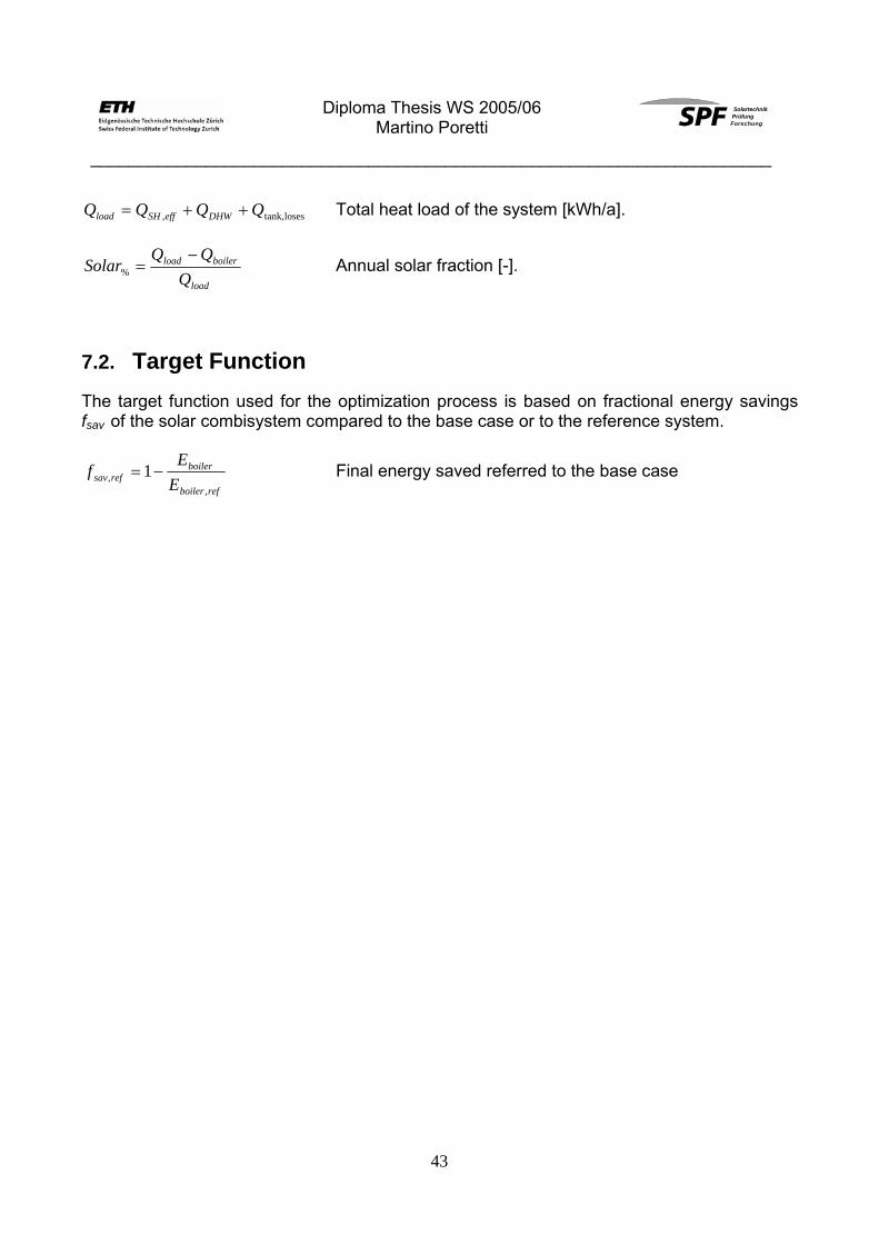
Diploma Thesis WS 2005/06
Martino Poretti SolartechnikPrüfungForschung
_______________________________________________________________________
43
losestank,, QQQQ DHWeffSHload ++= Total heat load of the system [kWh/a].
load
boilerload
QQQ
Solar−
=% Annual solar fraction [-].
7.2. Target Function The target function used for the optimization process is based on fractional energy savings fsav of the solar combisystem compared to the base case or to the reference system.
refboiler
boilerrefsav E
Ef
,, 1−= Final energy saved referred to the base case

Diploma Thesis WS 2005/06
Martino Poretti SolartechnikPrüfungForschung
_______________________________________________________________________
44
8. Validation of the model 8.1. Time step For all the simulations a time step of 3 minutes is chosen. The models don’t allow to change it because otherwise the space heating file is not read correctly. The timestep selected is be a good compromise between accuracy and simulation speed.
8.2. Convergence and integral tolerances The TRNSYS models accuracy calculation is evaluated by varying the convergence and integral tolerance from 0.1 to 0.001. It is decided that the necessary accuracy is obtained when the differences in fsav , QSH , QBoiler, Eboiler , Esolar between actual and previous run are below 0.2%. As Table 8-1 to Table 8-4 show, an integral and convergence accuracy value of 0.01 are chosen.
8.2.1. Direct Deed Flow Controlled
Table 8-1: Influence of the TRNSYS convergence and integral tolerances
Integration and Convergence tolerance QSH [kWh] QBoiler [kWh] Eboiler [kWh] Esolar [kWh] fsav,ref [%]
0.05 -8324.76 8789.34 8385.89 4266.25 -0.698
0.04 -8345.68 8807.15 8400.06 4271.36 -0.869
0.03 -8325.78 8788.51 8360.13 4271.71 -0.389
0.02 -8355.87 8815.99 8344.20 4275.96 -0.198
0.01 -8358.02 8813.70 8327.73 4283.49 0.000
0.005 -8358.73 8808.50 8319.62 4289.52 0.097
0.001 -8359.64 8809.09 8321.62 4288.28 0.073
0.0005 -8362.03 8812.04 8324.92 4287.30 0.034
0.0001 -8363.13 8813.32 8326.06 4286.66 0.020
Table 8-2: Difference caused by the convergence and the integral tolerances variation
Relative difference Integration and Convergence tolerance QSH [kWh] QBoiler [kWh] Eboiler [kWh] Esolar [kWh] fsav,ref [%]
0.04 0.251% 0.202% 0.169% 0.120% 0.170%
0.03 -0.239% -0.212% -0.478% 0.008% 0.480%
0.02 0.360% 0.312% -0.191% 0.099% 0.191%
0.01 0.026% -0.026% -0.198% 0.176% 0.198%
0.005 0.009% -0.059% -0.097% 0.141% 0.097%
0.001 0.011% 0.007% 0.024% -0.029% 0.024%
0.0005 0.029% 0.033% 0.040% -0.023% 0.040%
0.0001 0.013% 0.014% 0.014% -0.015% 0.014%

Diploma Thesis WS 2005/06
Martino Poretti SolartechnikPrüfungForschung
_______________________________________________________________________
45
8.2.2. Reference model
Table 8-3: Influence of the TRNSYS convergence and integral tolerances
Integration and Convergence tolerance QSH [kWh] QBoiler [kWh] Eboiler [kWh] Esolar [kWh] fsav,ref [%]
0.05 -8332.86 8927.05 8556.25 4144.15 -2.74
0.04 -8334.17 8922.05 8542.11 4155.56 -2.57
0.03 -8338.20 8920.56 8531.66 4158.16 -2.45
0.02 -8338.33 8914.73 8524.53 4164.43 -2.36
0.01 -8345.23 8915.19 8522.71 4170.96 -2.34
0.005 -8347.51 8907.49 8512.83 4180.85 -2.22
0.001 -8331.85 8895.23 8497.71 4176.96 -2.04
0.0005 -8330.53 8894.38 8495.81 4176.49 -2.02
0.0001 -8328.38 8894.33 8492.70 4174.15 -1.98
Table 8-4: Difference caused by the convergence and the integral tolerances variation
Relative difference Integration and Convergence tolerance QSH [kWh] QBoiler [kWh] Eboiler [kWh] Esolar [kWh] fsav,ref [%]
0.04 0.016% -0.056% -0.165% 0.275% 0.170%
0.03 0.048% -0.017% -0.122% 0.063% 0.125%
0.02 0.002% -0.065% -0.084% 0.150% 0.086%
0.01 0.083% 0.005% -0.021% 0.157% 0.022%
0.005 0.027% -0.086% -0.116% 0.236% 0.119%
0.001 -0.188% -0.138% -0.178% -0.093% 0.181%
0.0005 -0.016% -0.010% -0.022% -0.011% 0.023%
0.0001 -0.026% -0.001% -0.037% -0.056% 0.037%

Diploma Thesis WS 2005/06
Martino Poretti SolartechnikPrüfungForschung
_______________________________________________________________________
46
8.3. Energy balance The energy balance of the calculation is checked at the chosen tolerance of 0.01 and with a time step of 3 minutes.
8.3.1. Direct Feed Flow Controlled
Table 8-5: Energy balance of the Direct Feed Flow Controlled System
Energy supplied from gas boiler to heating media (Qboiler) 8813.698 kWh
Energy supplied from collector loop to storage (Qsolar,usable) 4283.49 kWh
Energy in 13097.19 kWh
Energy supplied from tank to space heating loop (QSH,eff) -8358.02 kWh
DHW consumption (QDHW) -3038.43 kWh
Energy loses storage tank (Qtank,loses) -1680.11 kWh
Energy out -13076.6 kWh Difference in-out 20.632 kWh Relative difference 0.158 %
8.3.2. Reference model
Table 8-6: Energy balance of the Reference Model
Energy supplied from gas boiler to heating media (Qboiler) 8915.19 kWh
Energy supplied from collector loop to storage (Qsolar,usable) 4170.96 kWh
Energy in 13086.15 kWh
Energy supplied from tank to space heating loop (QSH,eff) -8345.23 kWh
DHW consumption (QDHW) -3036.89 kWh
Energy loses storage tank (Qtank,loses) -1683.78 kWh
Energy out -13065.91 kWh Difference in-out 20.247 kWh Relative difference 0.155 %

Diploma Thesis WS 2005/06
Martino Poretti SolartechnikPrüfungForschung
_______________________________________________________________________
47
9. Sensitivity analysis and optimization 9.1. Introduction In order to optimize the two concept systems described in the previous sections and to check how they behave under different conditions a sensitivity analysis is performed. The study is executed starting from the base case of the systems and varying a parameter or maximal two at the same time maintaining the other constant to check how the model reacts.
9.2. Boiler Type 269 analyses The auxiliary boiler is probably the most sensitive part of the simulated systems. It follows that the results of a good optimization depend most of all on it. For this reason in this chapter the performances of this unit are analyzed in detail. The parameters of the boiler unit TRNSYS non-standard Type 269 are them described in section 5.3.4. The inputs used as basis case in this chapter are described in Table 9-1. During this tests the boiler model is simulated alone in a separated TRNSYS deck file without any other element.
Table 9-1: Basis case inputs of the boiler stand alone analysis
Boiler basis case inputs Set supply temperature (DHW and SH) 65 °C Water supply mass flow rate 200 kg/h Cold water temperature 30°C Air surplus number (λ) 1.2 Hysteresis for Tset 5 °C Air temperature 15°C Fuel type Natural gas
9.2.1. Steady state
The first analysis is performed on the boiler running in steady state condition. The auxiliary heater is maintained always on but allowing power modulation between 30% and 100%. Figure 9-1 shows the boiler efficiency as function of the feed water temperature entering the boiler. As the curve illustrates the efficiency is strongly dependent on the feed water temperature flowing into the boiler. In Figure 9-2 is plotted the efficiency as function of the boiler mass flow rate. For a fix value of the feed water temperature entering the boiler the efficiency variation due to the change in the mass flow is not so relevant.
In Figure 9-3 and Figure 9-4 is shown the thermal energy percent gain due to the exiting gas flue condensation. The curves demonstrate a relevant dependence on the boiler feed water temperature. Other side for a set fix water temperature of 30 °C (basis case) the condensation gain isn’t much dependent of the mass flow rate trough the boiler.

Diploma Thesis WS 2005/06
Martino Poretti SolartechnikPrüfungForschung
_______________________________________________________________________
48
Boiler Efficiency (ηboiler)
94%
96%
98%
100%
102%
104%
106%
108%
110%
112%
0 10 20 30 40 50 60
Water temperature entering the boiler [°C]
Effic
ienc
y [%
]
Figure 9-1: Boiler efficiency vs. feed water temperature
Boiler Efficiency (ηboiler)
105.3%
105.4%
105.5%
105.6%
105.7%
105.8%
105.9%
106.0%
106.1%
0 100 200 300 400 500
Water mass flow entering the boiler [kg/h]Ef
ficie
ncy
[%]
Figure 9-2: Boiler efficiency vs. water mass flow rate
Condensation Gain
0.0
1.0
2.0
3.0
4.0
5.0
6.0
7.0
8.0
9.0
10.0
10 15 20 25 30 35 40 45 50 55
Temperature of water entering the boiler [°C]
Con
dens
atio
n G
ain
[%]
Figure 9-3: Condensation gain vs. feed water temperature
Condensation Gain
7.55
7.58
7.60
7.63
7.65
7.68
7.70
7.73
7.75
50 100 150 200 250 300 350 400 450
Mass flow of water entering the boiler [kg/h]
Con
dens
atio
n G
ain
[%]
Figure 9-4: Condensation gain vs. water mass flow
As Figure 9-5 shows, for a different lambda value (varied from 1.0 to 1.3), a change in the boiler efficiency is only relevant for an high feed water temperature, condition that makes the boiler modulate the power at a very low level.
Figure 9-6 demonstrates hat the boiler efficiency is about 0.4-0.6% higher when the combustion air temperature is 10°C higher than the basis case value, this effect is a consequence of the less energy loosed to heat the air in the combustion chamber.
For a mass flow of 200 Kg/h the efficiency of the boiler is not dependant on the boiler water supply set temperature as Figure 9-7 shows.

Diploma Thesis WS 2005/06
Martino Poretti SolartechnikPrüfungForschung
_______________________________________________________________________
49
Last test is performed to check which influence has the air humidity on the auxiliary heater efficiency. As the Figure 9-8 illustrates this parameter don’t have any effect on the boiler performance.
Boiler Efficiency
0.94
0.96
0.98
1.00
1.02
1.04
1.06
1.08
1.10
0 10 20 30 40 50 60
Water temperature entering the boiler [°C]
Effic
ienc
y [%
]
Base case(Lambda 1.2)
Lambda 1.0
Lambda 1.1
Lambda 1.3
Figure 9-5: Boiler efficiency as function of the feed water
temperature and the lambda value
Boiler Efficiency
94%
96%
98%
100%
102%
104%
106%
108%
110%
0 10 20 30 40 50 60Water temperature entering
the boiler [°C]
Effic
ienc
y [%
]
Base case (airTemp. 15°C)
Air temp. 25°C
Figure 9-6: Boiler efficiency as function of the feed water
temperature and the combustion air temperature
Boiler Efficiency
0.94
0.96
0.98
1.00
1.02
1.04
1.06
1.08
1.10
0 10 20 30 40 50 60
Water temperature entering the boiler [°C]
Effic
ienc
y [%
]
Base case set.temp. 65°CSet temp. 60°C
Set temp. 70°C
Figure 9-7: Boiler efficiency as function of the feed water
temperature and the set supply temperature
Boiler Efficency
0.94
0.96
0.98
1.00
1.02
1.04
1.06
1.08
1.10
0 10 20 30 40 50 60
Water temperature entering the boiler [°C]
Effic
ency
[%]
Base case
Relativehumidity 0.0
Relativehumidity 1.0
Figure 9-8: Boiler efficiency as function of the feed water temperature and the relative humidity of the air

Diploma Thesis WS 2005/06
Martino Poretti SolartechnikPrüfungForschung
_______________________________________________________________________
50
9.2.2. Unsteady state
A second analysis is performed when the boiler is operating in an “unsteady state”. As “Unsteady state” is described the condition when the boiler runs in a sequence of on-off cycles. This conditions might appear when the temperature of the water flowing into the boiler is very high and near its set supply temperature, or it could happen when the pump mass flow rate of the auxiliary heater is very low. Both of these conditions make the boiler run at the minimum of the allowed modulation power (in this case 30% of the maximum power: equivalent to 3.5 kW). In case that the minimum power is still too high, so to make the temperature at the boiler outlet rise more than 5°C higher than the set temperature, the gas firing is stopped until the supply temperature reaches the set value again.
Figure 9-9 shows the change between steady and unsteady state caused by the rise of the temperature of the water entering the boiler. As the curve demonstrates the efficiency continues approximately the same curve plotted for the steady state boiler run.
In Figure 9-10 is represented the boiler efficiency curve as function of the mass flow rate flowing through the auxiliary heater. In this case to maintain a set temperature of 65°C the boiler, because of the on-off cycles, shows a wavering curve with a maximum boiler efficiency variation in the order of 0.8%.
Figure 9-9: Boiler efficiency as function of the water feed temperature

Diploma Thesis WS 2005/06
Martino Poretti SolartechnikPrüfungForschung
_______________________________________________________________________
51
Figure 9-10: Boiler efficiency as function of the boiler mass flow rate
9.2.3. Conclusion
The results of the boiler operation analysis of section 9.2.1 and 9.2.2 show that the new boiler model (TRNSYS non-standard Type 269) created by Michel Haller satisfies all the operational condition and its outputs could be considered plausible in all the working conditions.

Diploma Thesis WS 2005/06
Martino Poretti SolartechnikPrüfungForschung
_______________________________________________________________________
52
9.3. Direct Feed Flow Controlled system parameter analysis
9.3.1. Introduction
In this section is presented a complete parameter analysis of the Direct Feed Flow Controlled system described in chapter 5. The goal is to find possibility of optimization and to check the solidity of the simulation model. The study is subdivided into the main parts of the system: Auxiliary heater, storage tank, collector loop, space heating loop and domestic hot water.
The value of the saving function is always referred to the basis case of the Direct Feed Flow Controlled system. A positive value of the saving function means a better overall system efficiency than that of the basis case (see section 7.2)
9.3.2. Auxiliary heater
As said before the auxiliary heater is probably the most sensitive part of the entire system, only achieving to understand how the model behave in different situations can lead to a real possibility of system optimization. The followings parameter were analyzed:
Storage tank outlet to the auxiliary heater
The first parameter analysis has as goal to determine the optimum storage outlet position to the boiler, trying to find a good compromise between the solar and the boiler efficiency. Both the two heat sources have a better efficiency when they are fed with low temperature water, they are so in a kind of “competition”.
Figure 9-12 shows the boiler efficiency (ηboiler) and the solar fraction (solar%). As was predictable the two curves have opposite course. For a lower position of the storage outlet to the boiler, therefore a lower temperature of the water entering the auxiliary heater, the boiler have an higher efficiency but “steals” some point to the solar part. For an higher outlet position the net solar gain is higher but the performance of the auxiliary heater drop down. So it’s necessary to find a compromise between both heat sources efficiency.
The correlation between a lower outlet port position (lower water temperature) and a better boiler efficiency is due to a better energy gain from the condensation of the gas flue exiting the auxiliary heater as Figure 9-13 shows.

Diploma Thesis WS 2005/06
Martino Poretti SolartechnikPrüfungForschung
_______________________________________________________________________
53
Boiler efficiency and condensation gain
104.6%
104.8%
105.0%
105.2%
105.4%
105.6%
105.8%
106.0%
106.2%
106.4%
106.6%
0 0.1 0.2 0.3 0.4 0.5 0.6
Storage tank outlet relative position
Effic
ienc
y [%
]
680
690
700
710
720
730
740
750
760
770
780
Con
dens
atio
n ga
in [k
Wh]
BoilerefficiencyCondensationgain kWh
Figure 9-13: Boiler efficiency and condensation gain as
function of the relative position of the storage outlet to the boiler
As Figure 9-11 illustrates the best compromise between the performances of the heat sources is given at a relative outlet height of 0.4-0.45. This value isn’t far from the base case value of 0.4, that can already be considered as optimized.
Saving function
-1.6%
-1.4%
-1.2%
-1.0%
-0.8%
-0.6%
-0.4%
-0.2%
0.0%
0.2%
0.05 0.1 0.15 0.2 0.25 0.3 0.35 0.4 0.45 0.5 0.55Storage tank outlet relative position
Sav
ing
func
tion
[%]
Figure 9-11: Saving function as function of the relative
position of the storage outlet to the boiler
Solar fraction and boiler efficiency
31.2%
31.4%
31.6%
31.8%
32.0%
32.2%
32.4%
32.6%
32.8%
33.0%
0 0.1 0.2 0.3 0.4 0.5 0.6Relative position tank outlet
Effic
ienc
y [%
]
104.6%
104.8%
105.0%
105.2%
105.4%
105.6%
105.8%
106.0%
106.2%
106.4%
106.6%
Solar efficiency
Boiler fraction
Figure 9-12: Solar fraction and boiler efficiency as
function of the relative position of the storage outlet to the boiler

Diploma Thesis WS 2005/06
Martino Poretti SolartechnikPrüfungForschung
_______________________________________________________________________
54
Table 9-2: Simulation results as function of the relative height of the storage outlet to the boiler
Parameter [-]
QSH,target
[kWh/a]QSH,eff
[kWh/a]Qsolar,tank
[kWh/a]Qsolar,loses
[kWh/a]Qboiler
[kWh/a]Eboiler
[kWh/a]QDHW
[kWh/a]VDHW40
[l/a]Qtank,loses
[kWh/a]Qcond,gain
[kWh/a]nboiler
[1/a]tboiler
[kWh/a]Solar%
[%]ηboiler [%] fsav [%]
0.10 -8379 -8359 4147 645 8987 8442 -3039 0 -1712 771 4286 1672 31.4% 106.5% -1.37%0.20 -8379 -8360 4213 639 8910 8383 -3039 0 -1700 758 4569 1701 32.0% 106.3% -0.67%0.30 -8379 -8359 4248 635 8861 8351 -3038 0 -1690 747 4802 1731 32.3% 106.1% -0.28%0.35 -8379 -8359 4267 632 8836 8336 -3038 0 -1684 741 4988 1752 32.5% 106.0% -0.10%0.40 -8379 -8358 4283 632 8814 8328 -3038 0 -1680 733 5242 1782 32.6% 105.8% 0.00%0.45 -8379 -8356 4302 629 8786 8325 -3039 0 -1673 719 5879 1849 32.8% 105.5% 0.03%0.50 -8379 -8349 4317 627 8759 8356 -3039 0 -1670 686 7906 2010 32.9% 104.8% -0.34%
Relative height of the tank outlet to the auxiliary heater
Auxiliary heater minimal modulation range
Allowing the auxiliary heater to run at very low power levels should reduce the number of boiler starts significantly. In this case, as Figure 9-15 shows, if the minimal boiler power is reduced under 30% of the maximal power, there are no further significant reduction in the number of boiler starts. This is due to the relative high boiler set temperature and boiler mass flow rate. These factors practically don’t permit to the boiler to run at lower modulation range also when it would be possible. Another cause is the low feed water temperature entering the boiler which make the heat power needed increase.
If the minimal allowed power of the running boiler is raised above 30% of the maximal power, the number of boiler starts grow exponentially as we can see in Figure 9-15. There isn’t any correlation between boiler starts and boiler efficiency in the simulation model, but in reality there should be a sink in efficiency for a very high number of boiler starts.
Saving function
-0.5%
-0.4%
-0.3%
-0.2%
-0.1%
0.0%
0.1%
0.2%
0.3%
0.4%
0.5%
0% 5% 10% 15% 20% 25% 30% 35% 40% 45%Boiler minimal modulation range [%]
Sav
ing
func
tion
[%]
Figure 9-14: Saving function as function of the minimal
modulation range of the gas boiler
Boiler efficiency and boiler starts
104.0%
104.5%
105.0%
105.5%
106.0%
106.5%
107.0%
107.5%
108.0%
0% 10% 20% 30% 40% 50%Boiler minimal modulation range [%]
Boi
ler e
ffici
ency
[%]
0
5000
10000
15000
20000
25000
30000
35000
40000
45000
Boiler efficiency
Boiler starts
Figure 9-15: Boiler efficiency and number of boiler starts as function of the minimal modulation range of the gas
boiler

Diploma Thesis WS 2005/06
Martino Poretti SolartechnikPrüfungForschung
_______________________________________________________________________
55
Table 9-3: Simulation results as function of the minimal modulation range of the gas boiler
Parameter [%]
QSH,target
[kWh/a]QSH,eff
[kWh/a]Qsolar,tank
[kWh/a]Qsolar,loses
[kWh/a]Qboiler
[kWh/a]Eboiler
[kWh/a]QDHW
[kWh/a]VDHW40
[l/a]Qtank,loses
[kWh/a]Qcond,gain
[kWh/a]nboiler
[1/a]tboiler
[kWh/a]Solar%
[%]ηboiler [%] fsav [%]
4.2% -8379 -8358 4283 631 8814 8323 -3039 0 -1679 732 3892 1782 32.6% 105.9% 0.05%8.3% -8379 -8358 4283 631 8814 8323 -3039 0 -1679 732 3892 1782 32.6% 105.9% 0.05%16.7% -8379 -8358 4283 631 8814 8323 -3039 0 -1679 732 3892 1782 32.6% 105.9% 0.05%29.2% -8379 -8358 4283 632 8814 8328 -3038 0 -1680 733 5242 1782 32.6% 105.8% 0.00%33.3% -8379 -8359 4290 631 8809 8328 -3038 0 -1682 733 10147 1776 32.6% 105.8% 0.00%41.7% -8379 -8359 4291 630 8816 8330 -3038 0 -1690 736 42546 1741 32.6% 105.8% -0.03%
Minimal modulation range of the auxiliary heater
Boiler mass flow rate for the DHW charging loop
As shown in chapter 9.2.1 the boiler mass flow rate could bring an increase of the boiler efficiency if optimized. As described in section 5.4.2 the auxiliary heater has two differed charging cycles, one for the domestic hot water and another for the space heating charging loop. Figure 9-16 illustrates how the boiler behaves when the mass flow rate for the DHW charging loop is changed. As the plotted curve shows in this case any improvement in the boiler efficiency is noticeable for both lowering o increasing the mass flow rate.
During this analysis the auxiliary heater mass flow rate for the space heating charging loop remain the same as in the basis case.
Saving function and boiler efficiency
-1.0%
-0.8%
-0.6%
-0.4%
-0.2%
0.0%
0.2%
0.4%
75 125 175 225 275
Boiler mass flow rate DHW loading loop [kg/h]
Sav
ing
func
tion
[%]
105.0%
105.3%
105.5%
105.8%
106.0%
106.3%
106.5%
106.8%
107.0%
Effi
cien
cy [%
]
Saving function
Boiler efficiency
Figure 9-16: Saving function and boiler efficiency as function of
the boiler mass flow rate for the DHW charging loop

Diploma Thesis WS 2005/06
Martino Poretti SolartechnikPrüfungForschung
_______________________________________________________________________
56
Table 9-4: : Simulation results as function of the boiler mass flow rate for the DHW charging loop
Parameter [kg/h]
QSH,target
[kWh/a]QSH,eff
[kWh/a]Qsolar,tank
[kWh/a]Qsolar,loses
[kWh/a]Qboiler
[kWh/a]Eboiler
[kWh/a]QDHW
[kWh/a]VDHW40
[l/a]Qtank,loses
[kWh/a]Qcond,gain
[kWh/a]nboiler
[1/a]tboiler
[kWh/a]Solar%
[%]ηboiler [%] fsav [%]
100 -8379 -8354 4283 630 8809 8324 -3038 0 -1679 733 7343 1860 32.6% 105.8% 0.05%125 -8379 -8356 4284 631 8811 8325 -3038 0 -1679 733 6076 1828 32.6% 105.8% 0.04%150 -8379 -8357 4284 631 8811 8325 -3038 0 -1679 733 5525 1809 32.6% 105.8% 0.03%175 -8379 -8358 4287 631 8809 8324 -3038 0 -1679 733 5214 1793 32.6% 105.8% 0.05%200 -8379 -8358 4283 632 8814 8328 -3038 0 -1680 733 5242 1782 32.6% 105.8% 0.00%225 -8379 -8359 4282 631 8816 8330 -3038 0 -1680 733 5424 1779 32.6% 105.8% -0.02%
Boiler mass flow rate for the DHW charging loop
Boiler mass flow rate for the space heating charging loop
In the base case of the Direct Feed Flow Controlled system the mass flow rate of the boiler, when operating for the space heating charging loop, is a function of the space heating pump flow rate and it follows the relation given by Equation 9-1 (as described in section 5.4.2).
SHAUXm ,& = SHm& + C Equation 9-1
The “plus” factor given by the constant C for the base case is set to 30 kg/h. Figure 9-18 shows how the boiler efficiency and the solar fraction change if the value of C is varied. As is demonstrated by Figure 9-17 the optimum value of C is between 30-35 kg/h, it follows that the chosen basis case value of 30 kg/h can considered as already optimized.
Saving function
-1.00%
-0.80%
-0.60%
-0.40%
-0.20%
0.00%
0.20%
0.40%
0.60%
0.80%
1.00%
15 20 25 30 35 40 45 50 55Boiler mass flow rate "plus" coefficent for SH loading loop [kg/h]
Sav
ing
func
tion
[%]
Figure 9-17: Saving function as function of the C
constant
Boiler efficiency and solar fraction
105.0%
105.3%
105.5%
105.8%
106.0%
106.3%
106.5%
106.8%
107.0%
10 20 30 40 50 60Boiler flow rate "plus" coefficent for SH loading
loop [kg/h]
Effi
cien
cy [%
]
31.0%
31.3%
31.5%
31.8%
32.0%
32.3%
32.5%
32.8%
33.0%
Boiler efficiency
Solarfraction
Figure 9-18: Boiler efficiency and solar fraction as
function of the C constant

Diploma Thesis WS 2005/06
Martino Poretti SolartechnikPrüfungForschung
_______________________________________________________________________
57
Table 9-5: Simulation results as function of the C constant
Parameter [kg/h]
QSH,target
[kWh/a]QSH,eff
[kWh/a]Qsolar,tank
[kWh/a]Qsolar,loses
[kWh/a]Qboiler
[kWh/a]Eboiler
[kWh/a]QDHW
[kWh/a]VDHW40
[l/a]Qtank,loses
[kWh/a]Qcond,gain
[kWh/a]nboiler
[1/a]tboiler
[kWh/a]Solar%
[%]ηboiler [%] fsav [%]
75 -8379 -8092 4281 632 8555 8096 -3038 0 -1686 710 11484 2263 33.2% 105.7% 2.78%80 -8379 -8162 4281 632 8619 8154 -3038 0 -1680 713 6002 2196 33.1% 105.7% 2.09%85 -8379 -8216 4283 632 8668 8197 -3038 0 -1678 718 3140 2105 33.0% 105.7% 1.57%90 -8379 -8242 4282 632 8696 8222 -3038 0 -1677 720 2916 2014 32.9% 105.8% 1.27%95 -8379 -8270 4284 632 8721 8244 -3038 0 -1677 723 3157 1925 32.8% 105.8% 1.01%
100 -8379 -8292 4283 632 8746 8265 -3038 0 -1677 726 3411 1840 32.8% 105.8% 0.75%125 -8379 -8360 4283 632 8814 8327 -3039 0 -1678 732 4454 1504 32.6% 105.8% 0.01%150 -8379 -8383 4283 632 8837 8349 -3039 0 -1678 734 5192 1275 32.5% 105.8% -0.26%175 -8379 -8400 4285 631 8854 8365 -3039 0 -1678 735 5690 1110 32.5% 105.8% -0.45%200 -8379 -8415 4285 631 8868 8379 -3039 0 -1678 736 6239 985 32.5% 105.8% -0.62%225 -8379 -8429 4285 631 8882 8393 -3039 0 -1678 737 6430 888 32.4% 105.8% -0.79%250 -8379 -8438 4284 632 8893 8405 -3040 0 -1679 737 6274 811 32.4% 105.8% -0.93%300 -8379 -8446 4269 633 8898 8415 -3037 0 -1665 730 6187 770 32.3% 105.7% -1.05%350 -8379 -8448 4252 635 8905 8440 -3035 250 -1655 717 6172 819 32.2% 105.5% -1.35%400 -8379 -8434 4235 638 8918 8472 -3036 293 -1665 700 5565 912 32.1% 105.3% -1.74%
Constant boiler mass flow rate for the SH charging loop (C parameter)
Instead of a variable mass flow rate of the boiler when it operates controlled by the space heating sensor (sensor 2) it’s now tried to maintain this flow constant as Equation 9-2 describes.
SHAUXm ,& = D Equation 9-2
Figure 9-19 and Figure 9-20 show the saving function, the solar fraction and the boiler efficiency for different values of the constant D.
For a constant value of SHAUXm ,& it seems that the overall system efficiency is higher but as Figure 9-21 demonstrates the energy delivered to the space heating is not constant and differs from the goal value of 8379 kWh is some cases for more than 3.5%. It is so impossible to make a fair comparison.

Diploma Thesis WS 2005/06
Martino Poretti SolartechnikPrüfungForschung
_______________________________________________________________________
58
Saving function
-2.0%
-1.5%
-1.0%
-0.5%
0.0%
0.5%
1.0%
1.5%
2.0%
2.5%
3.0%
3.5%
50 100 150 200 250 300 350 400 450Boiler constant flow rate for SH loading loop [kg/h]
Sav
ing
func
tion
[%]
Figure 9-19: Saving function as function of the D constant
Boiler efficiency and solar fraction
105.2%
105.3%
105.4%
105.5%
105.6%
105.7%
105.8%
105.9%
50 100 150 200 250 300 350 400 450Boiler constant flow rate for SH loading loop [kg/h]
Effi
cien
cy [%
]
32.0%
32.2%
32.4%
32.6%
32.8%
33.0%
33.2%
33.4%
Boiler efficiency
Solar fraction
Figure 9-20: Boiler efficiency and solar fraction as function of the D constant
Energy for space heating
8000
8100
8200
8300
8400
8500
8600
50 150 250 350 450Boiler constant flow rate for SH loading loop [kg/h]
Spa
ce h
eatin
g en
ergy
[kW
h]
Goal value
Effective SHEnergy
Figure 9-21: Heat energy delivered by the space heating as
function of the D constant
Table 9-6: Simulation results as function of the D constant
Parameter [kg/h]
QSH,target
[kWh/a]QSH,eff
[kWh/a]Qsolar,tank
[kWh/a]Qsolar,loses
[kWh/a]Qboiler
[kWh/a]Eboiler
[kWh/a]QDHW
[kWh/a]VDHW40
[l/a]Qtank,loses
[kWh/a]Qcond,gain
[kWh/a]nboiler
[1/a]tboiler
[kWh/a]Solar%
[%]ηboiler [%] fsav [%]
20 -8379 -8356 4287 631 8811 8329 -3038 0 -1682 734 10235 1964 32.6% 105.8% -0.02%25 -8379 -8357 4284 632 8812 8329 -3038 0 -1681 733 6981 1869 32.6% 105.8% -0.01%30 -8379 -8358 4283 632 8814 8328 -3038 0 -1680 733 5242 1782 32.6% 105.8% 0.00%35 -8379 -8360 4283 632 8816 8327 -3039 0 -1679 732 4575 1704 32.6% 105.9% 0.00%40 -8379 -8364 4283 632 8819 8330 -3039 0 -1679 733 4477 1633 32.6% 105.9% -0.03%50 -8379 -8372 4283 632 8827 8336 -3039 0 -1679 733 4701 1508 32.6% 105.9% -0.10%
Boiler mass flow rate D parameter for the SH charging loop

Diploma Thesis WS 2005/06
Martino Poretti SolartechnikPrüfungForschung
_______________________________________________________________________
59
Boiler set temperature
Next analysis is performed on the set supply temperature of the auxiliary heater. As Figure 9-23 shows a slight increase of the boiler efficiency is noticeable rising the supply temperature. Figure 9-23 demonstrates that this boiler efficiency increase don’t lead to any final energy saving improvement of the system. The cause is probably to be found in the increased heat loses of the storage tank, compensating so the higher boiler efficiency. A set supply temperature optimum value is found between 62 and 67 °C. It follows that the chosen set temperature of 65°C for the base case can already de considered as optimized.
Saving function
-1.0%
-0.8%
-0.6%
-0.4%
-0.2%
0.0%
0.2%
58 60 62 64 66 68 70 72
Boiler supply set temperature [°C]
Sav
ing
func
tion
[%]
Figure 9-22: Saving function as function of the
boiler set supply temperature
Tank loses and boiler efficiency
-2.5%
-2.0%
-1.5%
-1.0%
-0.5%
0.0%
0.5%
1.0%
1.5%
58 60 62 64 66 68 70 72Boiler supply set temperature [°C]
Sav
ing
in ta
nk lo
ses
[%]
105.1%
105.2%
105.3%
105.4%
105.5%
105.6%
105.7%
105.8%
105.9%
Boi
ler e
ffici
ency
[%]
Tank loses
Boiler efficiency
Figure 9-23: Storage loses and boiler efficiency as function of
the boiler set supply temperature
Table 9-7: Simulation results as function of the boiler set supply temperature
Parameter [°C]
QSH,target
[kWh/a]QSH,eff
[kWh/a]Qsolar,tank
[kWh/a]Qsolar,loses
[kWh/a]Qboiler
[kWh/a]Eboiler
[kWh/a]QDHW
[kWh/a]VDHW40
[l/a]Qtank,loses
[kWh/a]Qcond,gain
[kWh/a]nboiler
[1/a]tboiler
[kWh/a]Solar%
[%]ηboiler [%] fsav [%]
60 -8379 -8361 4243 637 8842 8406 -3036 0 -1659 698 7814 1952 32.3% 105.2% -0.95%62 -8379 -8360 4275 632 8806 8329 -3037 0 -1664 724 5455 1854 32.6% 105.7% -0.01%65 -8379 -8358 4283 632 8814 8328 -3038 0 -1680 733 5242 1782 32.6% 105.8% 0.00%67 -8379 -8359 4294 631 8816 8328 -3039 0 -1691 736 5368 1739 32.6% 105.9% -0.01%70 -8379 -8359 4289 630 8843 8353 -3039 0 -1712 741 5165 1660 32.6% 105.9% -0.31%
Boiler set temperature for DHW and SH

Diploma Thesis WS 2005/06
Martino Poretti SolartechnikPrüfungForschung
_______________________________________________________________________
60
9.3.3. Storage tank
Cut off temperature in storage tank
The maximum allowed temperature inside the storage tank and it’s influence on the overall system efficiency is of major interest for the Direct Feed Flow Controlled system. Most of all to check if a cheap plastic-made storage with a limited maximal temperature have an negative repercussion on the overall solar gain.
During the operation the maximum temperature inside the tank is only reached when there’s lot of sun and the solar collectors are working at full load, this means when it were possible to increase the solar gain.
Figure 9-24 and Figure 9-25 show the variation of the saving function and the solar fraction by changing the cut off temperature in the storage tank. As it’s demonstrated limiting the maximum storage tank temperature by 70°C about 3.0% more final energy (gas) is needed and the overall solar fraction is about 3.5% lower.
These results are interesting because they show that also in the worst case, strongly limiting the temperature inside the storage, the drop in the saving function isn’t so pronounced. The explanation is to be found in the fact that the system, also with a limited maximal allowed temperature, can practically cover the domestic hot water load during the sunny months. During the heating season instead the collectors don’t have the capacity to heat the storage above 70°C it follows that the maximal storage tank temperature is never reached.
Saving function
-3.5%
-3.0%
-2.5%
-2.0%
-1.5%
-1.0%
-0.5%
0.0%
0.5%
65 70 75 80 85 90 95 100
Cut off temperature in storage tank [°C]
Sav
ing
func
tion
[%]
Figure 9-24: Saving function as function of the cut off temperature in the storage tank
Solar fraction
29.0%
29.5%
30.0%
30.5%
31.0%
31.5%
32.0%
32.5%
33.0%
65 70 75 80 85 90 95 100Cut off temperature in storage tank [°C]
Sol
ar fr
actio
n [%
]
Figure 9-25: Solar fraction as function of the cut off
temperature in the storage tank
In Figure 9-26 are plotted the storage tank and the collector pipes loses in function of the storage cut off temperature.

Diploma Thesis WS 2005/06
Martino Poretti SolartechnikPrüfungForschung
_______________________________________________________________________
61
Collector pipes and tank loses
300
350
400
450
500
550
600
650
65 70 75 80 85 90 95 100
Cut off temperature in storage tank [°C]
Col
lect
or p
ipes
lose
s [k
Wh]
1400
1450
1500
1550
1600
1650
1700
Sto
rage
tank
lose
s [k
Wh]
Collector pipeslosesStorage tankloses
Figure 9-26: Collector pipes and storage tank loses as
function of the cut off temperature in the storage
Table 9-8: Simulation results as function of the cut off temperature in the storage tank
Parameter [°C]
QSH,target
[kWh/a]QSH,eff
[kWh/a]Qsolar,tank
[kWh/a]Qsolar,loses
[kWh/a]Qboiler
[kWh/a]Eboiler
[kWh/a]QDHW
[kWh/a]VDHW40
[l/a]Qtank,loses
[kWh/a]Qcond,gain
[kWh/a]nboiler
[1/a]tboiler
[kWh/a]Solar%
[%]ηboiler [%] fsav [%]
65 -8379 -8363 1081 161 11489 10867 -3038 133 -1148 960 8736 2371 8.5% 105.7% -30.50%70 -8379 -8358 3787 457 9049 8571 -3038 0 -1419 745 5272 1840 29.4% 105.6% -2.92%75 -8379 -8358 3991 496 8907 8425 -3038 0 -1481 737 5323 1806 30.8% 105.7% -1.17%80 -8379 -8358 4094 537 8871 8390 -3038 63 -1549 735 5162 1795 31.5% 105.7% -0.74%85 -8379 -8358 4191 570 8827 8343 -3038 0 -1602 733 5231 1786 32.1% 105.8% -0.18%90 -8379 -8358 4256 604 8815 8330 -3038 0 -1655 733 5244 1783 32.5% 105.8% -0.03%95 -8379 -8358 4283 632 8814 8328 -3038 0 -1680 733 5242 1782 32.6% 105.8% 0.00%
Storage tank cut off temperature
Storage tank volume
The volume of the storage tank has a big influence on the cost of the solar combisystem. In this section the effect of the this parameter variation is analyzed referred to the overall energy efficiency of the system. Table 9-9 shows how the storage tank loss coefficient is recalculated in function of the usable volume. The DHW sensor (sensor 1), as all other parameters such as the inlet and outlet ports and sensors relative height are maintained unaltered. It follows that the volume reserved for the DHW varies in function of the overall storage tank volume (third colon of Table 9-9).

Diploma Thesis WS 2005/06
Martino Poretti SolartechnikPrüfungForschung
_______________________________________________________________________
62
Table 9-9: Storage loses coefficient and DHW reserved volume as function of the total storage tank volume
Storage Volume [Liters]
Loses coefficient [kJ/h]
DHW volume [liters]
400 13.84 120 500 14.98 150 600 16.11 180 700 17.10 210 800 18.08 240 900 18.97 270
1000 19.86 300 1100 20.70 330 1200 21.53 360
As Figure 9-28 demonstrates, varying the storage volume from 400 to 1200 liter a solar fraction change from 29% to 36% is noticeable. The saving function don’t vary much also for big difference in storage tank volume compared to the base case.
As Figure 9-27 shows the auxiliary final energy saved with a storage volume increased by 50% (from 800 to 1200 liters) is only about 0.7%. This fact is to conduct to the higher storage tank loses derived by a bigger volume that aren’t balanced by a so high solar gain. This fact is illustrated by Figure 9-29.
Saving function
-5.0%
-4.5%
-4.0%
-3.5%
-3.0%
-2.5%
-2.0%
-1.5%
-1.0%
-0.5%
0.0%
0.5%
1.0%
300 400 500 600 700 800 900 1000 1100 1200 1300Storage tank voulme [l]
Sav
ing
func
tion
Figure 9-27: Saving function as function of the storage
tank total volume
Solar fraction
27%
28%
29%
30%
31%
32%
33%
34%
35%
300 400 500 600 700 800 900 1000 1100 1200 1300
Storage tank voulme [l]
Sol
ar fr
actio
n [%
]
Figure 9-28: Solar fraction as function of the storage tank
total volume

Diploma Thesis WS 2005/06
Martino Poretti SolartechnikPrüfungForschung
_______________________________________________________________________
63
Energy difference form base case
-800
-600
-400
-200
0
200
400
600
300 400 500 600 700 800 900 1000 1100 1200 1300
Storage tank voulme [l]
Ene
rgy
diffe
renc
e [k
Wh]
Tank loses difference frombase case
Solar collector gaindifference form base case
Figure 9-29: Energy difference from the base case as
function of the storage tank volume
Table 9-10: Simulation results as function of the storage tank total volume
Parameter [liters]
QSH,target
[kWh/a]QSH,eff
[kWh/a]Qsolar,tank
[kWh/a]Qsolar,loses
[kWh/a]Qboiler
[kWh/a]Eboiler
[kWh/a]QDHW
[kWh/a]VDHW40
[l/a]Qtank,loses
[kWh/a]Qcond,gain
[kWh/a]nboiler
[1/a]tboiler
[kWh/a]Solar%
[%]ηboiler [%] fsav [%]
400 -8379 -8408 3570 664 9167 8689 -3038 55 -1281 749 7649 1706 28.0% 105.5% -4.34%500 -8379 -8356 3797 657 9022 8563 -3038 55 -1413 734 6611 1907 29.5% 105.4% -2.83%600 -8379 -8358 4004 648 8917 8444 -3038 0 -1509 735 6056 1859 30.9% 105.6% -1.40%700 -8379 -8358 4146 639 8867 8388 -3039 0 -1598 734 5332 1803 31.8% 105.7% -0.72%800 -8379 -8358 4283 632 8814 8328 -3038 0 -1680 733 5242 1782 32.6% 105.8% 0.00%900 -8379 -8343 4379 626 8797 8325 -3038 0 -1771 727 5739 1879 33.1% 105.7% 0.04%1000 -8379 -8343 4480 622 8781 8299 -3038 0 -1853 730 5666 1863 33.6% 105.8% 0.34%1100 -8379 -8342 4565 616 8768 8287 -3038 0 -1923 728 4870 1837 34.1% 105.8% 0.49%1200 -8379 -8342 4654 612 8753 8269 -3038 0 -1995 728 4860 1824 34.6% 105.9% 0.70%
Storage tank volume
9.3.4. Collector loop
Collector area
The first parameter analysis that concern the collector loop is the variation of the collector area. As expected the solar fraction increases for a bigger collector area, from a 50% bigger collector area there’s a solar fraction increase of 5.5 % and a final energy saving of about 7% (Figure 9-30).
The effective final energy saving of the auxiliary heater per year should be compared to the higher investment costs caused by an higher collector area to find a cost-related optimized value.

Diploma Thesis WS 2005/06
Martino Poretti SolartechnikPrüfungForschung
_______________________________________________________________________
64
Saving function
-15%
-10%
-5%
0%
5%
10%
15%
4 6 8 10 12 14 16 18 20 22Collector area [m2]
Sav
ing
func
tion
[%]
Figure 9-30: Saving function as function of the collector area
Solar gain
20%
23%
25%
28%
30%
33%
35%
38%
40%
43%
45%
4 6 8 10 12 14 16 18 20 22Collector area [m2]
Sol
ar g
ain
[%]
Figure 9-31: Solar fraction as function of the collector area
Table 9-11: Simulation results as function of the collector area
Parameter [m2]
QSH,target
[kWh/a]QSH,eff
[kWh/a]Qsolar,tank
[kWh/a]Qsolar,loses
[kWh/a]Qboiler
[kWh/a]Eboiler
[kWh/a]QDHW
[kWh/a]VDHW40
[l/a]Qtank,loses
[kWh/a]Qcond,gain
[kWh/a]nboiler
[1/a]tboiler
[kWh/a]Solar%
[%]ηboiler [%] fsav [%]
6 -8379 -8360 2870 483 9947 9417 -3037 133 -1399 823 6143 2038 22.3% 105.6% -13.08%8 -8379 -8359 3461 558 9483 8970 -3038 0 -1527 786 5790 1935 26.6% 105.7% -7.72%10 -8379 -8359 3909 601 9116 8617 -3038 0 -1608 757 5351 1844 29.9% 105.8% -3.47%12 -8379 -8358 4283 632 8814 8328 -3038 0 -1680 733 5242 1782 32.6% 105.8% 0.00%14 -8379 -8358 4586 654 8575 8100 -3039 0 -1744 713 4989 1727 34.7% 105.9% 2.73%16 -8379 -8357 4836 665 8365 7901 -3038 0 -1785 696 4946 1688 36.5% 105.9% 5.12%18 -8379 -8356 5047 680 8191 7738 -3038 0 -1823 681 4769 1651 38.0% 105.9% 7.08%20 -8379 -8356 5244 687 8026 7582 -3038 0 -1854 667 4614 1614 39.4% 105.9% 8.96%
Collector area
Collector a1 coefficient
Another parameter that is analyzed is the solar collector efficiency parameter a1. This parameter is varied form the base case value of 3.5 W/m2.K to a optimal value of 1.0 W/m2.K. This study is very theoretical because so low a1 coefficients are practically not reachable with standard collectors. The result of the saving function and solar fraction are show by the Figure 9-32 and Figure 9-33 respectively.

Diploma Thesis WS 2005/06
Martino Poretti SolartechnikPrüfungForschung
_______________________________________________________________________
65
Saving function
-1%
0%
1%
2%
3%
4%
5%
6%
7%
8%
9%
0.5 1.0 1.5 2.0 2.5 3.0 3.5 4.0Collector's a1 coefficent [W/m2.K]
Sav
ing
func
tion
[%]
Figure 9-32: Saving function as function of the
collector a1 coefficient
Solar fraction
32%
33%
34%
35%
36%
37%
38%
39%
0.5 1.0 1.5 2.0 2.5 3.0 3.5 4.0Collector's a1 coefficent [W/m2.K]
Sola
r fra
ctio
n [%
]
Figure 9-33: Solar fraction as function of the collector a1
coefficient
Table 9-12: Simulation results as function of the collector a1 coefficient
Parameter [W/m2.K]
QSH,target
[kWh/a]QSH,eff
[kWh/a]Qsolar,tank
[kWh/a]Qsolar,loses
[kWh/a]Qboiler
[kWh/a]Eboiler
[kWh/a]QDHW
[kWh/a]VDHW40
[l/a]Qtank,loses
[kWh/a]Qcond,gain
[kWh/a]nboiler
[1/a]tboiler
[kWh/a]Solar%
[%]ηboiler [%] fsav [%]
3.50 -8379 -8358 4283 632 8814 8328 -3038 0 -1680 733 5242 1782 32.6% 105.8% 0.00%3.00 -8379 -8358 4445 653 8679 8200 -3039 0 -1708 722 4968 1750 33.8% 105.8% 1.53%2.50 -8379 -8358 4571 668 8558 8085 -3039 0 -1712 711 4987 1726 34.7% 105.8% 2.92%2.00 -8379 -8357 4719 691 8429 7964 -3039 0 -1732 700 4824 1697 35.8% 105.8% 4.36%1.50 -8379 -8356 4884 712 8281 7827 -3038 110 -1751 687 4716 1667 37.0% 105.8% 6.02%1.00 -8379 -8356 5060 734 8124 7679 -3038 110 -1769 673 4580 1636 38.3% 105.8% 7.79%
Collector a1 coefficent
Collector loop pump flow rate
The collector loop pump flow rate is varied to check if there are possible optimizations in the solar fraction or in the overall system efficiency. During the analysis the variations of the pump flow rate are maintained small, so that the collector loop can always be considered as a low flow system.
The results are show in Figure 9-34 and Figure 9-35 respectively. The system optimum referred to the saving function is reached for a value of 10 kg/h, it means 2 kg/h lower than the basis case value, however the gain is minimal, in the order of 2 ‰.

Diploma Thesis WS 2005/06
Martino Poretti SolartechnikPrüfungForschung
_______________________________________________________________________
66
Saving function
-1.4%
-1.2%
-1.0%
-0.8%
-0.6%
-0.4%
-0.2%
0.0%
0.2%
0.4%
4 6 8 10 12 14 16 18 20Collector pump flow rate [kg/m2.h]
Sav
ing
func
tion
[%]
Figure 9-34: Saving function as function of the collector
pump flow rate
Solar fraction
30.0%
30.5%
31.0%
31.5%
32.0%
32.5%
33.0%
4 6 8 10 12 14 16 18 20Collector pump flow rate [kg/m2.h]
Sav
ing
func
tion
[%]
Figure 9-35: Solar fraction as function of the collector pump
flow rate
Table 9-13: Simulation results as function of the collector pump flow rate
Parameter [kg/h.m2]
QSH,target
[kWh/a]QSH,eff
[kWh/a]Qsolar,tank
[kWh/a]Qsolar,loses
[kWh/a]Qboiler
[kWh/a]Eboiler
[kWh/a]QDHW
[kWh/a]VDHW40
[l/a]Qtank,loses
[kWh/a]Qcond,gain
[kWh/a]nboiler
[1/a]tboiler
[kWh/a]Solar%
[%]ηboiler [%] fsav [%]
6 -8379 -8359 3958 554 8931 8438 -3038 0 -1471 744 5021 1807 30.6% 105.8% -1.32%8 -8379 -8358 4169 589 8811 8323 -3038 55 -1565 734 5034 1779 32.0% 105.9% 0.05%10 -8379 -8358 4262 618 8798 8310 -3038 0 -1643 733 5117 1774 32.5% 105.9% 0.21%12 -8379 -8358 4283 632 8814 8328 -3038 0 -1680 733 5242 1782 32.6% 105.8% 0.00%14 -8379 -8358 4293 639 8823 8338 -3038 0 -1700 733 5249 1784 32.6% 105.8% -0.12%16 -8379 -8358 4289 641 8841 8354 -3039 0 -1712 735 5372 1792 32.6% 105.8% -0.32%18 -8379 -8359 4281 640 8857 8370 -3038 0 -1720 736 5405 1796 32.5% 105.8% -0.51%
Collector pump flow rate
Relative height of the storage inlet form the collector loop (without stratified charging mode)
In the following section is analyzed the influence that a fixed storage tank inlet has in comparison with the collector loop stratified charging mode.
In a stratified charged storage system the water coming from the solar collector enters the storage tank at the height where the water temperature inside the tank has the same temperature. During this analysis instead, the water from the collector loop enters the storage tank at a fix relative height that’s varied from 0.3 to 0.75.
As Figure 9-36 shows the optimum relative height for a fix solar inlet is about 0.4. Compared to the base case operating with a stratified charger, it’s noticeable that there’s a repercussion in the saving function of about -1.3%. This result is not so bad considering the lower cost of a storage tank without a stratified charging system.
It should be economically analyzed if the cost of a stratified charging system worth the small increase in the system performance.

Diploma Thesis WS 2005/06
Martino Poretti SolartechnikPrüfungForschung
_______________________________________________________________________
67
Saving function
-12.0%
-10.0%
-8.0%
-6.0%
-4.0%
-2.0%
0.0%
0.25 0.30 0.35 0.40 0.45 0.50 0.55 0.60 0.65 0.70 0.75 0.80Collector loop storage tank inlet relative height [-]
Sav
ing
func
tion
[%]
Figure 9-36: Saving function as function of the collector
loop storage inlet
Solar fraction and boiler efficiency
30.6%
30.8%
31.0%
31.2%
31.4%
31.6%
31.8%
32.0%
32.2%
0.05 0.15 0.25 0.35 0.45 0.55 0.65
Collector loop storage tank inlet relative height [-]
Effi
cien
cy [%
]
102.5%
103.0%
103.5%
104.0%
104.5%
105.0%
105.5%
106.0%
106.5%
Boi
ler e
ffici
ency
[%]
Solar fraction
Boiler efficency
Figure 9-37: Solar fraction and boiler efficiency as function
of the collector loop storage inlet
Table 9-14: Simulation results as function of the collector loop storage inlet
Parameter [-]
QSH,target
[kWh/a]QSH,eff
[kWh/a]Qsolar,tank
[kWh/a]Qsolar,loses
[kWh/a]Qboiler
[kWh/a]Eboiler
[kWh/a]QDHW
[kWh/a]VDHW40
[l/a]Qtank,loses
[kWh/a]Qcond,gain
[kWh/a]nboiler
[1/a]tboiler
[kWh/a]Solar%
[%]ηboiler [%] fsav [%]
0.30 -8379 -8359 4103 652 8939 8456 -3038 0 -1625 739 5548 1816 31.4% 105.7% -1.54%0.35 -8379 -8359 4123 650 8923 8443 -3038 0 -1629 737 5483 1814 31.5% 105.7% -1.38%0.40 -8379 -8359 4137 651 8917 8435 -3038 0 -1637 738 5372 1807 31.6% 105.7% -1.28%0.45 -8379 -8358 4139 652 8923 8440 -3038 0 -1645 738 5526 1811 31.6% 105.7% -1.35%0.50 -8379 -8358 4136 655 8930 8448 -3038 0 -1650 738 5620 1822 31.5% 105.7% -1.45%0.55 -8379 -8359 4084 664 8999 8524 -3037 0 -1667 738 9558 1895 31.1% 105.6% -2.35%0.60 -8379 -8357 4112 664 8971 8498 -3038 0 -1668 733 4678 1775 31.3% 105.6% -2.05%0.65 -8379 -8347 4078 667 9002 8541 -3038 0 -1675 730 4337 1761 31.1% 105.4% -2.56%0.70 -8379 -8351 3672 716 9508 9151 -3038 0 -1770 672 4190 1951 27.7% 103.9% -9.89%0.75 -8379 -8350 3671 714 9502 9157 -3038 0 -1765 663 4093 1969 27.8% 103.8% -9.96%
Tank inlet form collector loop without stratified charging
9.3.5. Domestic hot water
DHW reserved volume
In order to see how much must be the minimum water volume in the top of the storage tank reserved to the DHW to assure that a comfort is reached, the position of the sensor 1 has been varied form a relative height of 0.6 to 0.9. This variation represent a volume change from 320 to 80 liters respectively.
To analyze the DHW comfort a special check function is implemented in the simulation. This function gives at the end of the simulation an output that displays how many liters of water are supplied under the set comfort temperature value of 40°C.

Diploma Thesis WS 2005/06
Martino Poretti SolartechnikPrüfungForschung
_______________________________________________________________________
68
As the Figure 9-38 shows, for the given draw profile of 200 liter/day the volume of 240 liters reserved for DHW chosen for the base case, seems not the be necessary. As the parameter analysis illustrates, a volume of only 80 liters allows a final energy saving in the order of 3.5% with only a negative comfort of 55 liters under 40°C over an year (Figure 9-40).
Saving function
-3.0%
-2.5%
-2.0%
-1.5%
-1.0%
-0.5%
0.0%
0.5%
1.0%
1.5%
2.0%
2.5%
3.0%
3.5%
4.0%
50 100 150 200 250 300 350DHW reserved volume [l]
Sav
ing
func
tion
[%]
Figure 9-38: Saving function as function of the DHW reserved volume
Boiler efficiency and solar fraction
104.8%
105.0%
105.2%
105.4%
105.6%
105.8%
106.0%
106.2%
50 100 150 200 250 300 350DHW reserved volume [l]
Boi
ler e
ffici
ency
[%]
31.5%
32.0%
32.5%
33.0%
33.5%
34.0%
34.5%
Sol
ar fr
actio
n [%
]
Boiler efficiency
Solar fraction
Figure 9-39: Boiler efficiency and solar fraction as function
of the DHW reserved volume
DHW reserved volume
0.0
10.0
20.0
30.0
40.0
50.0
60.0
320 280 240 200 160 120 80DHW reserved volume [l]
Lite
r DH
W u
nder
40
°C
Figure 9-40: Liters of DHW that don’t match the comfort temperature of 40 °C over a year as function of the DHW
reserved volume
This result depends in large manner on the choice of the DHW heat exchanger. Using an external heat exchanger for DHW preparation as in this case shows that a much lower water volume maintained at an high temperature is needed to guarantee a satisfying DHW comfort.

Diploma Thesis WS 2005/06
Martino Poretti SolartechnikPrüfungForschung
_______________________________________________________________________
69
The results could have been different if an internal DHW heat exchanger were chosen, in such a case the amount of volume maintained at an higher temperature should have been probably higher. This option is not examined further.
Table 9-15: Simulation results as function of the DHW reserved volume
Parameter [kg/h]
QSH,target
[kWh/a]QSH,eff
[kWh/a]Qsolar,tank
[kWh/a]Qsolar,loses
[kWh/a]Qboiler
[kWh/a]Eboiler
[kWh/a]QDHW
[kWh/a]VDHW40
[l/a]Qtank,loses
[kWh/a]Qcond,gain
[kWh/a]nboiler
[1/a]tboiler
[kWh/a]Solar%
[%]ηboiler [%] fsav [%]
320 -8379 -8350 4214 639 8954 8539 -3039 0 -1755 703 7908 2048 31.9% 104.9% -2.53%280 -8379 -8356 4253 636 8882 8415 -3039 0 -1717 727 5720 1862 32.3% 105.5% -1.05%240 -8379 -8358 4283 632 8814 8328 -3038 0 -1680 733 5242 1782 32.6% 105.8% 0.00%200 -8379 -8358 4318 627 8739 8246 -3038 0 -1641 732 5065 1738 33.0% 106.0% 0.98%160 -8379 -8359 4349 623 8668 8175 -3038 0 -1603 730 5161 1709 33.3% 106.0% 1.83%120 -8379 -8360 4379 618 8596 8103 -3038 0 -1562 727 5179 1686 33.7% 106.1% 2.69%80 -8379 -8360 4408 615 8524 8034 -3036 55 -1521 724 5239 1673 34.0% 106.1% 3.52%
DHW reserved tank volume
DHW set temperature in storage tank
The set value of the water temperature in the storage tank reserved for the domestic hot water is varied from 50 to 64 °C to check how much energy can be saved. Figure 9-42 illustrates the comfort value in liter under 40°C (a 0 liters value is the optimum).
As Figure 9-41 demonstrates it’s possible to lower the temperature to 58°C without loosing any comfort and saving about 0.3 % of the final energy. Lowering the set temperature under this value leads to a loose in the DHW comfort. This negative effect is not so high, and can be considered as acceptable. The variation in the saving function is not so marked because the boiler supply set temperature remain 65°C, only the set temperature of the controller is varied.
Saving function
-2.0%
-1.5%
-1.0%
-0.5%
0.0%
0.5%
1.0%
49 50 51 52 53 54 55 56 57 58 59 60 61 62 63 64 65Storage tank set temperature for DHW [°C]
Sav
ing
func
tion
[%]
Figure 9-41: Saving function as function of the storage
tank set temperature for DHW
Storage tank set temperature for DHW
0
50
100
150
200
250
50 52 54 56 58 60 62 64Storage tank set temperature for DHW [°C]
Lite
rs D
HW
und
er 4
0°C
[l]
Figure 9-42: Liters of DHW that don’t match the comfort
temperature of 40 °C over a year as function of the storage tank set temperature for DHW
Table 9-16: Simulation results as function of the storage tank set temperature for DHW

Diploma Thesis WS 2005/06
Martino Poretti SolartechnikPrüfungForschung
_______________________________________________________________________
70
Parameter [°C]
QSH,target
[kWh/a]QSH,eff
[kWh/a]Qsolar,tank
[kWh/a]Qsolar,loses
[kWh/a]Qboiler
[kWh/a]Eboiler
[kWh/a]QDHW
[kWh/a]VDHW40
[l/a]Qtank,loses
[kWh/a]Qcond,gain
[kWh/a]nboiler
[1/a]tboiler
[kWh/a]Solar%
[%]ηboiler [%] fsav [%]
60 -8379 -8361 4243 637 8842 8406 -3036 0 -1659 698 7814 1952 32.3% 105.2% -0.95%62 -8379 -8360 4275 632 8806 8329 -3037 0 -1664 724 5455 1854 32.6% 105.7% -0.01%65 -8379 -8358 4283 632 8814 8328 -3038 0 -1680 733 5242 1782 32.6% 105.8% 0.00%67 -8379 -8359 4294 631 8816 8328 -3039 0 -1691 736 5368 1739 32.6% 105.9% -0.01%70 -8379 -8359 4289 630 8843 8353 -3039 0 -1712 741 5165 1660 32.6% 105.9% -0.31%
Boiler set temperature for DHW and SH
9.3.6. Space heating loop
Maximum allowed temperature in the space heating pipes
The maximum temperature allowed to flow in the space heating pipes must be in some heating systems technically lowered to reach and acceptable comfort or because of material problems.
In this paragraph the maximum allowed water temperature for the space heating supply is varied to check if there’s a change in the overall system efficiency. As Figure 9-43 illustrates, the saving function curve is practically constant. The small difference in the overall efficiency is probably correlated to a the smaller effective energy delivered by the space heating to the building.
As the results demonstrate it’s possible to limit the entering water temperature practically without loosing in the overall system efficiency.
Saving function and energy delivered by the SH
-0.4%
-0.3%
-0.2%
-0.1%
0.0%
0.1%
0.2%
0.3%
0.4%
40 45 50 55 60 65 70 75
Maximum allowed temperature in the space heating pipe [°C]
Sav
ing
func
tion
[%]
8320
8325
8330
8335
8340
8345
8350
8355
8360
8365
8370
SH
del
iver
ed e
nerg
y [k
Wh]
Saving function
SH effective energy
Figure 9-43: Saving function and energy delivered by the space heating as function of the maximum allowed water temperature
entering the space heating loop
Table 9-17: Simulation results as function of the maximum allowed mass flow rate of the space heating pump

Diploma Thesis WS 2005/06
Martino Poretti SolartechnikPrüfungForschung
_______________________________________________________________________
71
Parameter [°C]
QSH,target
[kWh/a]QSH,eff
[kWh/a]Qsolar,tank
[kWh/a]Qsolar,loses
[kWh/a]Qboiler
[kWh/a]Eboiler
[kWh/a]QDHW
[kWh/a]VDHW40
[l/a]Qtank,loses
[kWh/a]Qcond,gain
[kWh/a]nboiler
[1/a]tboiler
[kWh/a]Solar%
[%]ηboiler [%] fsav [%]
40 -8379 -8229 4262 634 8708 8272 -3038 0 -1683 692 6502 1165 32.8% 105.3% 0.67%45 -8379 -8343 4274 633 8811 8347 -3039 0 -1683 714 6111 1462 32.6% 105.6% -0.24%50 -8379 -8348 4281 632 8807 8328 -3038 0 -1681 726 5665 1677 32.6% 105.7% -0.01%55 -8379 -8358 4283 632 8814 8328 -3038 0 -1680 733 5242 1782 32.6% 105.8% 0.00%60 -8379 -8363 4285 632 8817 8330 -3038 0 -1680 734 5115 1800 32.6% 105.8% -0.03%65 -8379 -8363 4284 632 8818 8331 -3039 0 -1680 734 5111 1799 32.6% 105.8% -0.03%70 -8379 -8363 4285 632 8817 8330 -3038 0 -1680 734 5110 1799 32.6% 105.8% -0.03%
Maximum allowed temperature entering the SH pipe
Maximum allowed mass flow of the space heating pump
As Figure 9-44 shows the variation of the maximum mass flow rate of the space heating pump don’t have any influence in the overall efficiency. The results demonstrate that is possible to use a very low maximal mass flow rate and match the heat load demand during all the year with only minimal variations. It follows that an higher power pump with greater mass flow rate capability would never be used at the maximum of its capacity.
Saving function
-0.5%
-0.4%
-0.3%
-0.2%
-0.1%
0.0%
0.1%
0.2%
0.3%
0.4%
0.5%
100 200 300 400 500 600 700 800 900Maximal allowed mass flow of the space heating pump [kg/h]
Sav
ing
func
tion
[
Figure 9-44: Saving function as function of the maximum allowed mass flow entering the space heating pump
Table 9-18: Simulation results as function of the maximum allowed mass flow entering the space heating pump
Parameter [kg/h]
QSH,target
[kWh/a]QSH,eff
[kWh/a]Qsolar,tank
[kWh/a]Qsolar,loses
[kWh/a]Qboiler
[kWh/a]Eboiler
[kWh/a]QDHW
[kWh/a]VDHW40
[l/a]Qtank,loses
[kWh/a]Qcond,gain
[kWh/a]nboiler
[1/a]tboiler
[kWh/a]Solar%
[%]ηboiler [%] fsav [%]
200 -8379 -8346 4278 632 8816 8343 -3038 0 -1688 728 5531 1877 32.6% 105.7% -0.19%300 -8379 -8353 4282 632 8813 8331 -3038 0 -1682 732 5336 1815 32.6% 105.8% -0.04%400 -8379 -8358 4283 632 8814 8328 -3038 0 -1680 733 5242 1782 32.6% 105.8% 0.00%500 -8379 -8361 4285 631 8814 8326 -3038 0 -1679 733 5127 1762 32.6% 105.9% 0.02%600 -8379 -8363 4285 631 8815 8326 -3038 0 -1678 733 5131 1749 32.6% 105.9% 0.03%800 -8379 -8366 4286 631 8816 8326 -3039 0 -1677 734 5110 1734 32.6% 105.9% 0.02%
Maximum mass flow of the SH pump
Dead band space heating charging loop

Diploma Thesis WS 2005/06
Martino Poretti SolartechnikPrüfungForschung
_______________________________________________________________________
72
In this paragraph it’s checked which influence has the dead band value of the boiler sensor for the space heating on the overall system efficiency. The dead band value is varied from 2°C to 10°C. The difference caused by the variation of this parameter practically consist in the waited time before the auxiliary heater is started again to heat the storage tank water.
As the Figure 9-45 shows the improvement in the overall efficiency are practically unnoticeable. The base case can so be considered as already optimized.
Saving function
-0.4%
-0.3%
-0.2%
-0.1%
0.0%
0.1%
0.2%
0.3%
0.4%
1 2 3 4 5 6 7 8 9 10 11Dead band SH boiler charging loop [°C]
Sav
ing
func
tion
[%]
Figure 9-45: Saving function as function of the dead band during the SH charging loop
Table 9-19 Simulation results as function of the dead band during the SH charging loop
Parameter [°C]
QSH,target
[kWh/a]QSH,eff
[kWh/a]Qsolar,tank
[kWh/a]Qsolar,loses
[kWh/a]Qboiler
[kWh/a]Eboiler
[kWh/a]QDHW
[kWh/a]VDHW40
[l/a]Qtank,loses
[kWh/a]Qcond,gain
[kWh/a]nboiler
[1/a]tboiler
[kWh/a]Solar%
[%]ηboiler [%] fsav [%]
2 -8379 -8362 4290 631 8807 8318 -3039 0 -1676 733 9614 1728 32.7% 105.9% 0.11%3 -8379 -8359 4289 631 8806 8318 -3039 0 -1677 733 6963 1747 32.6% 105.9% 0.11%5 -8379 -8358 4283 632 8814 8328 -3038 0 -1680 733 5242 1782 32.6% 105.8% 0.00%6 -8379 -8356 4282 632 8815 8331 -3038 0 -1681 732 5098 1802 32.6% 105.8% -0.04%8 -8379 -8352 4277 633 8818 8338 -3038 0 -1685 731 4792 1831 32.6% 105.8% -0.12%10 -8379 -8348 4276 633 8819 8342 -3038 0 -1688 729 5497 1867 32.5% 105.7% -0.17%
Space heating charging loop dead band
Space heating storage tank sensor relative position
The position of the space heating storage tank sensor used by the auxiliary heater controller (sensor no. 2 Figure 5-10) is varied from 0.45 to 0.575. As Figure 9-46 shows there isn’t any improvement in the overall system efficiency. It seems that the optimum value is already reached in the base case (relative height of 0.55).
Figure 9-47 illustrates that there’s a correlation between the overall system efficiency and the numbers of boiler starts during a year.

Diploma Thesis WS 2005/06
Martino Poretti SolartechnikPrüfungForschung
_______________________________________________________________________
73
Saving function
-2.5%
-2.0%
-1.5%
-1.0%
-0.5%
0.0%
0.5%
0.425 0.450 0.475 0.500 0.525 0.550 0.575 0.600
Sapce heating sensor 2 relative position [-]
Sav
ing
func
tion
[%]
Figure 9-46: Saving function as function of the relative
position of the sensor 2 (SH)
Boiler starts
0
2000
4000
6000
8000
10000
12000
14000
16000
18000
20000
0.425 0.450 0.475 0.500 0.525 0.550 0.575 0.600Sapce heating sensor 2 relative position [-]
Boi
ler s
tarts
[%]
Figure 9-47: Boiler starts as function of the relative position of the sensor 2 (SH)
Table 9-20: Simulation results as function of the relative position of the sensor 2 (SH)
Parameter [-]
QSH,target
[kWh/a]QSH,eff
[kWh/a]Qsolar,tank
[kWh/a]Qsolar,loses
[kWh/a]Qboiler
[kWh/a]Eboiler
[kWh/a]QDHW
[kWh/a]VDHW40
[l/a]Qtank,loses
[kWh/a]Qcond,gain
[kWh/a]nboiler
[1/a]tboiler
[kWh/a]Solar%
[%]ηboiler [%] fsav [%]
0.450 -8379 -8338 4221 640 8914 8512 -3039 0 -1735 692 18079 2262 32.0% 104.7% -2.21%0.475 -8379 -8339 4243 637 8875 8439 -3039 0 -1718 709 12816 2127 32.2% 105.2% -1.34%0.500 -8379 -8338 4263 635 8839 8386 -3038 0 -1704 719 9472 2026 32.4% 105.4% -0.70%0.525 -8379 -8343 4272 633 8822 8352 -3038 0 -1692 728 6642 1919 32.5% 105.6% -0.30%0.550 -8379 -8358 4283 632 8814 8328 -3038 0 -1680 733 5242 1782 32.6% 105.8% 0.00%0.575 -8379 -8418 4293 630 8852 8357 -3039 0 -1668 736 6706 1571 32.6% 105.9% -0.35%
SH sensor position
Storage tank outlet to the space heating loop
During this analysis the storage tank outlet to the space heating loop is varied from the relative height of 0.5 to 0.7. The position of the space heating sensor is maintained in all simulation variants at a relative position of 0.05 lower than the storage tank outlet.
As the Figure 9-48 clearly illustrates there’s an optimum at the relative height of 0.65, it is also noticeable that at a relative height of 0.7 there’s a fall in the overall system efficiency. This effect is probably due to the fact that in this case the outlet port is at the same height as the storage tank sensor for the DHW, increasing also the number of the boiler starts.

Diploma Thesis WS 2005/06
Martino Poretti SolartechnikPrüfungForschung
_______________________________________________________________________
74
Saving function
-2.5%
-2.0%
-1.5%
-1.0%
-0.5%
0.0%
0.5%
1.0%
0.45 0.50 0.55 0.60 0.65 0.70 0.75
Space heating outlet port relative position [-]
Sav
ing
func
tion
[%]
Figure 9-48: Saving function as function of the space heating storage tank outlet
Solar fraction and boiler efficiency
31.9%
32.0%
32.1%
32.2%
32.3%
32.4%
32.5%
32.6%
32.7%
32.8%
32.9%
0.45 0.50 0.55 0.60 0.65 0.70 0.75Space heating outlet port relative position [-]
Sol
ar fr
actio
n [%
]
104.9%
105.0%
105.1%
105.2%
105.3%
105.4%
105.5%
105.6%
105.7%
105.8%
105.9%
106.0%
Boi
ler e
ffici
ency
[%]
Solar fraction
Boiler efficiency
Figure 9-49: Solar fraction and boiler efficiency as function
of the space heating storage outlet
Table 9-21: Simulation results as function of the space heating storage tank outlet
Parameter [-]
QSH,target
[kWh/a]QSH,eff
[kWh/a]Qsolar,tank
[kWh/a]Qsolar,loses
[kWh/a]Qboiler
[kWh/a]Eboiler
[kWh/a]QDHW
[kWh/a]VDHW40
[l/a]Qtank,loses
[kWh/a]Qcond,gain
[kWh/a]nboiler
[1/a]tboiler
[kWh/a]Solar%
[%]ηboiler [%] fsav [%]
0.500 -8379 -8352 4223 639 8938 8511 -3038 55 -1748 708 8343 2065 32.0% 105.0% -2.20%0.525 -8379 -8355 4241 636 8904 8445 -3038 0 -1729 723 6989 1951 32.1% 105.4% -1.41%0.550 -8379 -8357 4256 634 8872 8397 -3038 0 -1711 730 6409 1878 32.3% 105.7% -0.83%0.575 -8379 -8357 4277 633 8835 8354 -3038 0 -1695 732 5948 1830 32.5% 105.8% -0.32%0.600 -8379 -8358 4283 632 8814 8328 -3038 0 -1680 733 5242 1782 32.6% 105.8% 0.00%0.625 -8379 -8358 4293 630 8788 8301 -3038 0 -1665 732 4784 1735 32.7% 105.9% 0.32%0.650 -8379 -8357 4295 630 8774 8289 -3039 0 -1653 730 4271 1663 32.8% 105.8% 0.46%0.675 -8379 -8357 4283 631 8778 8302 -3039 0 -1648 726 3876 1561 32.7% 105.7% 0.31%0.700 -8379 -8353 4227 639 8857 8405 -3039 0 -1675 718 4514 1035 32.2% 105.4% -0.93%
SH outlet (sensor postioned always 0.05 lower)
Space heating storage tank inlet (without stratified charging mode)
In the following paragraph is analyzed the influence that a fixed storage tank inlet have in comparison with the stratified charging mode.
For a fixed space heating storage inlet the water from the space heating loop enters the storage tank at a fix relative height that is varied from 0.1 to 0.6. As the Figure 9-50 shows the optimum relative height is about 0.15-0.2.
In this optimized case the overall system efficiency drop is less than 1% compared to the stratified charging mode of the base case and it can be considered a good result.
Also in this case it should be economically analyzed if the cost of a stratified charging system worth the major gain in the system efficiency.
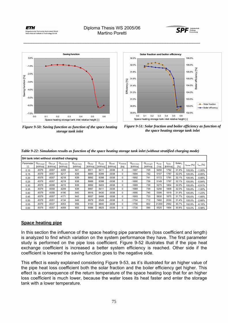
Diploma Thesis WS 2005/06
Martino Poretti SolartechnikPrüfungForschung
_______________________________________________________________________
75
Saving function
-7.0%
-6.0%
-5.0%
-4.0%
-3.0%
-2.0%
-1.0%
0.0%
0.0 0.1 0.2 0.3 0.4 0.5 0.6Space heating storage tank inlet relative height [-]
Sav
ing
func
tion
[%]
Figure 9-50: Saving function as function of the space heating storage tank inlet
Solar fraction and boiler efficiency
30.6%
30.8%
31.0%
31.2%
31.4%
31.6%
31.8%
32.0%
32.2%
0.0 0.1 0.2 0.3 0.4 0.5 0.6Space heating storage tank inlet relative height [-]
Effi
cien
cy [%
]
102.5%
103.0%
103.5%
104.0%
104.5%
105.0%
105.5%
106.0%
106.5%
Boi
ler e
ffici
ency
[%]
Solar fraction
Boiler efficency
Figure 9-51: Solar fraction and boiler efficiency as function of
the space heating storage tank inlet
Table 9-22: Simulation results as function of the space heating storage tank inlet (without stratified charging mode)
Parameter [-]
QSH,target
[kWh/a]QSH,eff
[kWh/a]Qsolar,tank
[kWh/a]Qsolar,loses
[kWh/a]Qboiler
[kWh/a]Eboiler
[kWh/a]QDHW
[kWh/a]VDHW40
[l/a]Qtank,loses
[kWh/a]Qcond,gain
[kWh/a]nboiler
[1/a]tboiler
[kWh/a]Solar%
[%]ηboiler [%] fsav [%]
0.10 -8379 -8357 4205 641 8911 8411 -3038 0 -1697 745 5450 1792 31.9% 105.9% -1.00%0.15 -8379 -8357 4217 639 8895 8399 -3038 0 -1694 742 5107 1787 32.0% 105.9% -0.85%0.20 -8379 -8357 4218 639 8892 8398 -3038 0 -1692 741 5172 1791 32.1% 105.9% -0.85%0.25 -8379 -8357 4219 638 8888 8398 -3038 0 -1690 739 5149 1797 32.1% 105.8% -0.84%0.30 -8379 -8358 4215 639 8892 8403 -3038 0 -1689 739 5275 1804 32.0% 105.8% -0.91%0.35 -8379 -8358 4209 639 8897 8411 -3038 0 -1689 739 5256 1809 32.0% 105.8% -1.00%0.40 -8379 -8358 4190 640 8916 8430 -3038 0 -1690 740 5306 1819 31.9% 105.8% -1.23%0.45 -8379 -8357 4171 642 8937 8466 -3038 0 -1693 733 5830 1875 31.7% 105.6% -1.66%0.50 -8379 -8351 4134 646 8979 8549 -3038 0 -1704 712 7460 2030 31.4% 105.0% -2.66%0.55 -8379 -8337 4053 656 9100 8840 -3038 0 -1756 602 31200 2562 30.7% 102.9% -6.16%0.60 -8379 -8357 4059 655 9088 8825 -3039 0 -1730 590 5525 1954 30.8% 103.0% -5.98%
SH tank inlet without stratified charging
Space heating pipe
In this section the influence of the space heating pipe parameters (loss coefficient and length) is analyzed to find which variation on the system performance they have. The first parameter study is performed on the pipe loss coefficient. Figure 9-52 illustrates that if the pipe heat exchange coefficient is increased a better system efficiency is reached. Other side if the coefficient is lowered the saving function goes to the negative side.
This effect is easily explained considering Figure 9-53, as it’s illustrated for an higher value of the pipe heat loss coefficient both the solar fraction and the boiler efficiency get higher. This effect is a consequence of the return temperature of the space heating loop that for an higher loss coefficient is much lower, because the water loses its heat faster and enter the storage tank with a lower temperature.
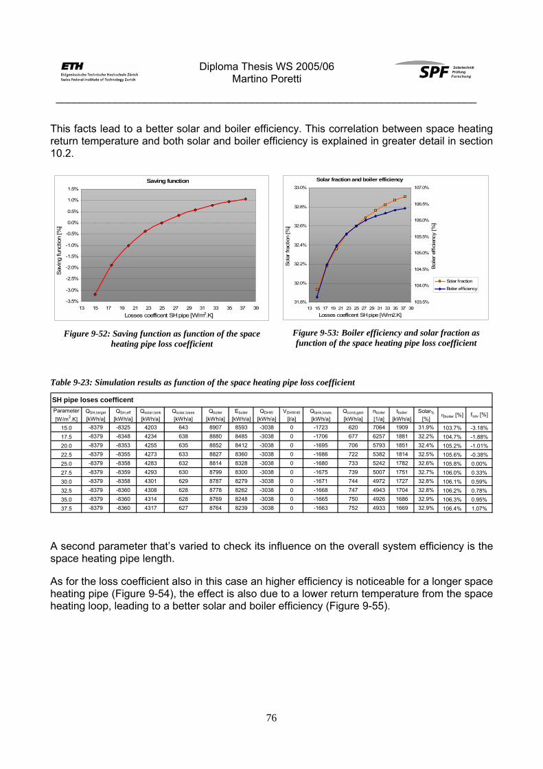
Diploma Thesis WS 2005/06
Martino Poretti SolartechnikPrüfungForschung
_______________________________________________________________________
76
This facts lead to a better solar and boiler efficiency. This correlation between space heating return temperature and both solar and boiler efficiency is explained in greater detail in section 10.2.
Saving function
-3.5%
-3.0%
-2.5%
-2.0%
-1.5%
-1.0%
-0.5%
0.0%
0.5%
1.0%
1.5%
13 15 17 19 21 23 25 27 29 31 33 35 37 39Losses coefficent SH pipe [W/m2.K]
Sav
ing
func
tion
[%]
Figure 9-52: Saving function as function of the space
heating pipe loss coefficient
Solar fraction and boiler efficiency
31.8%
32.0%
32.2%
32.4%
32.6%
32.8%
33.0%
13 15 17 19 21 23 25 27 29 31 33 35 37 39Losses coefficent SH pipe [W/m2.K]
Sol
ar fr
actio
n [%
]
103.5%
104.0%
104.5%
105.0%
105.5%
106.0%
106.5%
107.0%
Boi
ler e
ffici
ency
[%]
Solar fraction
Boiler efficiency
Figure 9-53: Boiler efficiency and solar fraction as function of the space heating pipe loss coefficient
Table 9-23: Simulation results as function of the space heating pipe loss coefficient
Parameter [W/m2.K]
QSH,target
[kWh/a]QSH,eff
[kWh/a]Qsolar,tank
[kWh/a]Qsolar,loses
[kWh/a]Qboiler
[kWh/a]Eboiler
[kWh/a]QDHW
[kWh/a]VDHW40
[l/a]Qtank,loses
[kWh/a]Qcond,gain
[kWh/a]nboiler
[1/a]tboiler
[kWh/a]Solar%
[%]ηboiler [%] fsav [%]
15.0 -8379 -8325 4203 643 8907 8593 -3038 0 -1723 620 7064 1909 31.9% 103.7% -3.18%17.5 -8379 -8348 4234 638 8880 8485 -3038 0 -1706 677 6257 1881 32.2% 104.7% -1.88%20.0 -8379 -8353 4255 635 8852 8412 -3038 0 -1695 706 5793 1851 32.4% 105.2% -1.01%22.5 -8379 -8355 4273 633 8827 8360 -3038 0 -1686 722 5382 1814 32.5% 105.6% -0.38%25.0 -8379 -8358 4283 632 8814 8328 -3038 0 -1680 733 5242 1782 32.6% 105.8% 0.00%27.5 -8379 -8359 4293 630 8799 8300 -3038 0 -1675 739 5007 1751 32.7% 106.0% 0.33%30.0 -8379 -8358 4301 629 8787 8279 -3038 0 -1671 744 4972 1727 32.8% 106.1% 0.59%32.5 -8379 -8360 4308 628 8778 8262 -3038 0 -1668 747 4943 1704 32.8% 106.2% 0.78%35.0 -8379 -8360 4314 628 8769 8248 -3038 0 -1665 750 4926 1686 32.9% 106.3% 0.95%37.5 -8379 -8360 4317 627 8764 8239 -3038 0 -1663 752 4933 1669 32.9% 106.4% 1.07%
SH pipe loses coefficent
A second parameter that’s varied to check its influence on the overall system efficiency is the space heating pipe length.
As for the loss coefficient also in this case an higher efficiency is noticeable for a longer space heating pipe (Figure 9-54), the effect is also due to a lower return temperature from the space heating loop, leading to a better solar and boiler efficiency (Figure 9-55).

Diploma Thesis WS 2005/06
Martino Poretti SolartechnikPrüfungForschung
_______________________________________________________________________
77
Saving function
-4.0%
-3.5%
-3.0%
-2.5%
-2.0%
-1.5%
-1.0%
-0.5%
0.0%
0.5%
1.0%
1.5%
30 40 50 60 70 80 90 100 110 120 130 140 150 160 170SH pipe lenght [m]
Sav
ing
func
tion
[%]
Figure 9-54: Saving function as function of the space
heating pipe length
Solar fraction and boiler efficiency
31.8%
32.0%
32.2%
32.4%
32.6%
32.8%
33.0%
25 50 75 100 125 150 175SH pipe lenght [m]
Sol
ar fr
actio
n [%
]
99%
100%
101%
102%
103%
104%
105%
106%
107%
Boi
ler e
ffici
ency
[%]
Solar fraction
Boiler efficiency
Figure 9-55: Boiler efficiency and solar fraction as
function of the space heating pipe length
Table 9-24: Simulation results as function of the space heating pipe length
Parameter [m]
QSH,target
[kWh/a]QSH,eff
[kWh/a]Qsolar,tank
[kWh/a]Qsolar,loses
[kWh/a]Qboiler
[kWh/a]Eboiler
[kWh/a]QDHW
[kWh/a]VDHW40
[l/a]Qtank,loses
[kWh/a]Qcond,gain
[kWh/a]nboiler
[1/a]tboiler
[kWh/a]Solar%
[%]ηboiler [%] fsav [%]
40.0 -8379 -7814 4091 656 8584 8627 -3038 0 -1794 354 14958 2132 32.1% 99.5% -3.59%60.0 -8379 -8317 4205 642 8896 8583 -3038 0 -1723 619 7096 1909 32.0% 103.6% -3.07%80.0 -8379 -8349 4257 635 8847 8407 -3038 0 -1695 705 5791 1850 32.4% 105.2% -0.96%100.0 -8379 -8358 4283 632 8814 8328 -3038 0 -1680 733 5242 1782 32.6% 105.8% 0.00%120.0 -8379 -8360 4301 629 8788 8280 -3038 0 -1671 744 4987 1727 32.8% 106.1% 0.58%140.0 -8379 -8362 4314 628 8771 8251 -3038 0 -1665 750 4923 1687 32.9% 106.3% 0.92%160.0 -8379 -8362 4320 627 8761 8232 -3038 0 -1661 754 4954 1654 32.9% 106.4% 1.15%
SH pipe lenght
Space heating load
To check how the model behaves under different space heating load conditions the input from the load file that represent the building is multiplied by a constant so to make the QSH,target value at the end of the year change. The base case load file represent a building which has an energy requirement of 60 kWh/m2a as described in section 5.3.6.
The base case is compared with other two variant, which represent a 30 kWh/m2a and 100 kWh/m2a building respectively. The heating power input of the load file is multiplied by 0.5 to replicate the 30 kWh/m2a variant and by 1.66 to simulate a 100 kWh/m2a house.
The results are resumed in table Table 9-25. As the ηsolar colon shows the boiler has a its best efficiency for the base case variant.

Diploma Thesis WS 2005/06
Martino Poretti SolartechnikPrüfungForschung
_______________________________________________________________________
78
Table 9-25: Simulation results as function of the space heating load
Parameter [kWh/m2a]
QSH,target
[kWh/a]QSH,eff
[kWh/a]Qsolar,tank
[kWh/a]Qsolar,loses
[kWh/a]Qboiler
[kWh/a]Eboiler
[kWh/a]QDHW
[kWh/a]VDHW40
[l/a]Qtank,loses
[kWh/a]Qcond,gain
[kWh/a]nboiler
[1/a]tboiler
[kWh/a]Solar%
[%]ηboiler [%] fsav [%]
30 -4190 -4148 4164 643 4737 4514 -3038 0 -1697 402 7296 1105 46.7% 104.9% 45.79%60 -8379 -8358 4283 632 8814 8328 -3038 0 -1680 733 5242 1782 32.6% 105.8% 0.00%
100 -13966 -13842 4319 629 14289 13704 -3039 0 -1703 981 5661 2315 23.1% 104.3% -64.56%
Space heating load
9.3.7. Conclusions
The detailed parameter analysis performed from section 9.3.1 to 9.3.6 on the Direct Feed Flow Controlled system concept shows that the system has a solid behavior. The choice of the base case parameters could be considered as practically optimized.
For some parameter as the collector area, the space heating length, and the storage tank stratified charging system a cost based analysis is necessary to find the cost related optimal values taking into account the higher or lower investment costs.

Diploma Thesis WS 2005/06
Martino Poretti SolartechnikPrüfungForschung
_______________________________________________________________________
79
9.4. Reference model parameter analysis
9.4.1. Introduction
In this section are presented the parameter analysis results of the reference model described in chapter 6. The goal is also here to find possibilities of optimization and to check the solidity of the simulation model. The parameters analyzed for the reference system are restricted to the sensor and port positions into the storage tank, the variation of the mass flow or the temperature of the auxiliary heater and the space heating loop parameters. The collector loop and the domestic hot water loop is no more investigated in detail.
The value of the saving function is always referred to the base case of the reference system described in section 6. A positive value of the saving function means a better system efficiency referred to the auxiliary final energy needed (see section 7.2)
9.4.2. Auxiliary heater
Storage tank outlet to the boiler
In this parameter study the height of the storage tank outlet to the boiler loop is changed from a relative height of 0.1 to a value of 0.5. The temperature sensor 1 used by the auxiliary heater controller in the storage tank it’s always placed at the same height as the outlet.
As it’s showed by the Figure 9-56 at a relative height of about 0.45 the maximal overall system efficiency is reached. A small change in the effective energy delivered to the building is noticeable so to make impossible to confirm the small saving function increase of only about 0.2%.
Saving function
-3.5%
-3.0%
-2.5%
-2.0%
-1.5%
-1.0%
-0.5%
0.0%
0.5%
0.05 0.10 0.15 0.20 0.25 0.30 0.35 0.40 0.45 0.50 0.55Relative height of the storage tank outlet to the boiler [-]
Sav
ing
func
tion
[%]
Figure 9-56: Saving function as function of the relative
height of the storage tank outlet to the boiler
Boiler efficiency and solar fraction
103.8%
104.0%
104.2%
104.4%
104.6%
104.8%
105.0%
105.2%
0.0 0.1 0.2 0.3 0.4 0.5 0.6Relative height of the storage tank outlet to the boiler [-]
Boi
ler e
ffici
ency
[%]
0.295
0.300
0.305
0.310
0.315
0.320
0.325
Sol
ar fr
actio
n [%
]
Boiler efficiency [%]
Solar fraction [%]
Figure 9-57: Boiler efficiency and solar fraction as
function of the relative height of the storage tank outlet to the boiler

Diploma Thesis WS 2005/06
Martino Poretti SolartechnikPrüfungForschung
_______________________________________________________________________
80
Table 9-26: Simulation results as function of the relative height of the storage tank outlet to the boiler
Parameter [-]
QSH,target
[kWh/a]QSH,eff
[kWh/a]Qsolar,tank
[kWh/a]Qsolar,loses
[kWh/a]Qboiler
[kWh/a]Eboiler
[kWh/a]QDHW
[kWh/a]VDHW40
[l/a]Qtank,loses
[kWh/a]Qcond,gain
[kWh/a]nboiler [1/a] tboiler
[kWh/a]Solar%
[%]ηboiler [%] fsav [%]
0.10 -8379 -8351 3940 669 9225 8775 -3037 0 -1750 699 932 1995 29.8% 105.1% -2.96%0.20 -8379 -8350 4058 658 9078 8650 -3038 0 -1725 681 1097 1991 30.8% 104.9% -1.50%0.30 -8379 -8349 4115 651 8997 8583 -3037 0 -1704 670 1358 1992 31.3% 104.8% -0.71%0.35 -8379 -8348 4145 648 8955 8553 -3037 110 -1694 662 1550 1998 31.5% 104.7% -0.36%0.40 -8379 -8354 4171 646 8924 8533 -3038 0 -1684 655 1800 2005 31.7% 104.6% 0.00%0.45 -8379 -8339 4193 643 8876 8503 -3038 0 -1673 645 2240 2021 32.0% 104.4% 0.23%0.50 -8379 -8326 4209 641 8837 8502 -3038 0 -1665 630 9611 2135 32.2% 103.9% 0.24%
Realtive position of the tank outlet to the boiler
Auxiliary heater mass flow rate for the space heating charging loop
In the base case of the reference model the mass flow rate of the boiler during the space heating charging loop is set to 400 kg/h. Figure 9-58 illustrates how the overall system efficiency varies by changing this parameter. The optimum is found at about 300 kg/h with am auxiliary final energy saving in the order of about 0.4%. Table 9-27 shows that also here the effective energy delivered to the building has some small variation so to make impossible a fair comparison most of all due to a so small gain in the saving function.
Saving function
-0.6%
-0.5%
-0.4%
-0.3%
-0.2%
-0.1%
0.0%
0.1%
0.2%
0.3%
0.4%
0.5%
200 250 300 350 400 450 500 550Auxiliary heater mass flow for the SH charging loop [kg/h]
Sav
ing
func
tion
[%]
Figure 9-58: Saving function as function of the boiler
mass flow rate during the SH charging loop.
Boiler efficiency
104.3%
104.4%
104.4%
104.5%
104.5%
104.6%
104.6%
104.7%
104.7%
104.8%
104.8%
200 250 300 350 400 450 500 550Auxiliary heater mass flow for the SH charging loop [kg/h]
Boi
ler e
ffici
ency
[%]
Figure 9-59:Boiler efficiency as function of the boiler
mass flow rate during the SH charging loop.
Table 9-27: Simulation results as function of the boiler mass flow rate during the SH charging loop.
Parameter [kg/h]
QSH,target
[kWh/a]QSH,eff
[kWh/a]Qsolar,tank
[kWh/a]Qsolar,loses
[kWh/a]Qboiler
[kWh/a]Eboiler
[kWh/a]QDHW
[kWh/a]VDHW40
[l/a]Qtank,loses
[kWh/a]Qcond,gain
[kWh/a]nboiler [1/a] tboiler
[kWh/a]Solar%
[%]ηboiler [%] fsav [%]
250 -8379 -8326 4168 646 8897 8496 -3037 0 -1683 658 64237 2422 31.8% 104.7% 0.31%300 -8379 -8331 4173 646 8897 8491 -3037 110 -1682 660 2628 2006 31.8% 104.8% 0.36%350 -8379 -8337 4174 645 8902 8503 -3038 0 -1681 657 1965 2003 31.8% 104.7% 0.23%400 -8379 -8354 4171 646 8924 8533 -3038 0 -1684 655 1800 2005 31.7% 104.6% 0.00%450 -8379 -8353 4167 646 8931 8546 -3038 0 -1686 652 1757 1990 31.7% 104.5% -0.28%500 -8379 -8356 4166 646 8935 8562 -3038 0 -1687 647 1769 1952 31.7% 104.4% -0.47%
Boiler mass flow for the SH charging loop

Diploma Thesis WS 2005/06
Martino Poretti SolartechnikPrüfungForschung
_______________________________________________________________________
81
9.4.3. Space heating loop
Relative position of the storage tank space heating temperature sensor
As the Figure 9-60 shows there are no possibilities of overall system efficiency improvement changing the relative position of the storage tank sensor 2 used by the auxiliary heater controller. The base case value of 0.6 can be considered as already optimized. If the sensor height is raised, is no more possible to match the space heat demand of the building as the QSH,eff colon in
Table 9-28 illustrates.
Saving function
-1.0%
-0.9%
-0.8%
-0.7%
-0.6%
-0.5%
-0.4%
-0.3%
-0.2%
-0.1%
0.0%
0.1%
0.450 0.475 0.500 0.525 0.550 0.575 0.600 0.625Realtive position of the SH temperature sensor [-]
Sav
ing
func
tion
[%]
Figure 9-60: Saving function as function of the position of the
sensor 2 used by the SH controller
Table 9-28: Simulation results as function of the position of the sensor 2 used by the SH controller
Parameter [-]
QSH,target
[kWh/a]QSH,eff
[kWh/a]Qsolar,tank
[kWh/a]Qsolar,loses
[kWh/a]Qboiler
[kWh/a]Eboiler
[kWh/a]QDHW
[kWh/a]VDHW40
[l/a]Qtank,loses
[kWh/a]Qcond,gain
[kWh/a]nboiler [1/a] tboiler
[kWh/a]Solar%
[%]ηboiler [%] fsav [%]
0.650 -8379 -3472 4258 634 3898 3709 -3038 0 -1630 328 595 436 52.1% 105.1% 56.41%0.625 -8379 -4842 4238 637 5301 5058 -3038 0 -1642 419 644 802 44.3% 104.8% 40.60%0.600 -8379 -8354 4171 646 8924 8533 -3038 0 -1684 655 1800 2005 31.7% 104.6% 0.00%0.575 -8379 -8346 4169 646 8920 8530 -3037 110 -1684 654 1978 2013 31.7% 104.6% -0.09%0.550 -8379 -8347 4166 646 8926 8539 -3038 0 -1687 652 2237 2019 31.7% 104.5% -0.19%0.525 -8379 -8346 4163 646 8930 8556 -3038 0 -1689 648 2321 2033 31.7% 104.4% -0.40%0.500 -8379 -8346 4159 647 8937 8572 -3037 0 -1692 642 2826 2056 31.7% 104.2% -0.59%0.475 -8379 -8347 4152 648 8949 8596 -3037 0 -1696 634 7128 2111 31.6% 104.1% -0.86%
Realtive position of the space heating temperature sensor 2

Diploma Thesis WS 2005/06
Martino Poretti SolartechnikPrüfungForschung
_______________________________________________________________________
82
Space heating outlet
The position of the storage tank outlet to the space heating loop is varied from the relative height position of 0.5 to 0.7. The space heating sensor used by the boiler controller is always placed at the same height as the storage outlet.
As Figure 9-61 illustrates there are no interesting possibility of optimization concerning this parameter.
Saving function
-1.80%
-1.60%
-1.40%
-1.20%
-1.00%
-0.80%
-0.60%
-0.40%
-0.20%
0.00%
0.20%
0.40%
0.475 0.500 0.525 0.550 0.575 0.600 0.625 0.650 0.675 0.700 0.725Space heating storage tank outlet height to the SH loop [-]
Sav
ing
func
tion
[%]
Figure 9-61: Saving function as functions of the relative
height of the storage tank outlet to the space heating
Table 9-29: Simulation results as function of the relative height of the storage tank outlet to the space heating
Parameter [°C]
QSH,target
[kWh/a]QSH,eff
[kWh/a]Qsolar,tank
[kWh/a]Qsolar,loses
[kWh/a]Qboiler
[kWh/a]Eboiler
[kWh/a]QDHW
[kWh/a]VDHW40
[l/a]Qtank,loses
[kWh/a]Qcond,gain
[kWh/a]nboiler [1/a] tboiler
[kWh/a]Solar%
[%]ηboiler [%] fsav [%]
0.500 -8379 -8310 4165 646 8903 8527 -3037 0 -1700 647 4114 2085 31.8% 104.4% -0.06%0.525 -8379 -8313 4163 646 8903 8517 -3037 110 -1697 651 3342 2071 31.8% 104.5% 0.06%0.550 -8379 -8326 4173 646 8903 8512 -3037 110 -1693 653 2771 2060 31.8% 104.6% 0.12%0.575 -8379 -8341 4163 647 8925 8530 -3037 0 -1690 656 2155 2034 31.7% 104.6% -0.09%0.600 -8379 -8354 4171 646 8924 8533 -3038 0 -1684 655 1800 2005 31.7% 104.6% 0.00%0.625 -8379 -8346 4173 645 8909 8518 -3038 0 -1678 655 1623 1963 31.8% 104.6% 0.06%0.650 -8379 -8347 4168 646 8911 8525 -3038 0 -1676 655 1590 1908 31.8% 104.5% -0.03%0.675 -8379 -8346 4160 647 8918 8545 -3039 0 -1675 656 1692 1764 31.7% 104.4% -0.26%0.700 -8379 -8360 4121 652 9004 8653 -3039 0 -1707 656 5239 1225 31.3% 104.1% -1.53%
Space heating tank outlet
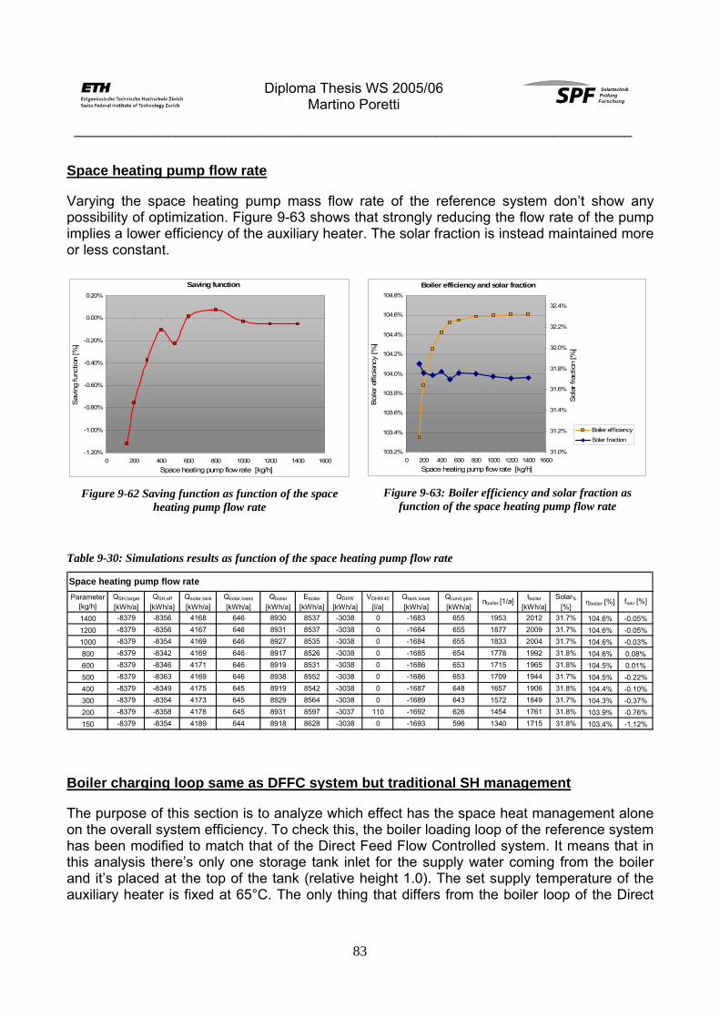
Diploma Thesis WS 2005/06
Martino Poretti SolartechnikPrüfungForschung
_______________________________________________________________________
83
Space heating pump flow rate
Varying the space heating pump mass flow rate of the reference system don’t show any possibility of optimization. Figure 9-63 shows that strongly reducing the flow rate of the pump implies a lower efficiency of the auxiliary heater. The solar fraction is instead maintained more or less constant.
Saving function
-1.20%
-1.00%
-0.80%
-0.60%
-0.40%
-0.20%
0.00%
0.20%
0 200 400 600 800 1000 1200 1400 1600Space heating pump flow rate [kg/h]
Sav
ing
func
tion
[%]
Figure 9-62 Saving function as function of the space
heating pump flow rate
Boiler efficiency and solar fraction
103.2%
103.4%
103.6%
103.8%
104.0%
104.2%
104.4%
104.6%
104.8%
0 200 400 600 800 1000 1200 1400 1600Space heating pump flow rate [kg/h]
Boi
ler e
ffici
ency
[%]
31.0%
31.2%
31.4%
31.6%
31.8%
32.0%
32.2%
32.4%
Sol
ar fr
actio
n [%
]
Boiler efficiency
Solar fraction
Figure 9-63: Boiler efficiency and solar fraction as
function of the space heating pump flow rate
Table 9-30: Simulations results as function of the space heating pump flow rate
Parameter [kg/h]
QSH,target
[kWh/a]QSH,eff
[kWh/a]Qsolar,tank
[kWh/a]Qsolar,loses
[kWh/a]Qboiler
[kWh/a]Eboiler
[kWh/a]QDHW
[kWh/a]VDHW40
[l/a]Qtank,loses
[kWh/a]Qcond,gain
[kWh/a]nboiler [1/a] tboiler
[kWh/a]Solar%
[%]ηboiler [%] fsav [%]
1400 -8379 -8356 4168 646 8930 8537 -3038 0 -1683 655 1953 2012 31.7% 104.6% -0.05%1200 -8379 -8356 4167 646 8931 8537 -3038 0 -1684 655 1877 2009 31.7% 104.6% -0.05%1000 -8379 -8354 4169 646 8927 8535 -3038 0 -1684 655 1833 2004 31.7% 104.6% -0.03%800 -8379 -8342 4169 646 8917 8526 -3038 0 -1685 654 1778 1992 31.8% 104.6% 0.08%600 -8379 -8346 4171 646 8919 8531 -3038 0 -1686 653 1715 1965 31.8% 104.5% 0.01%500 -8379 -8363 4169 646 8938 8552 -3038 0 -1686 653 1709 1944 31.7% 104.5% -0.22%400 -8379 -8349 4175 645 8919 8542 -3038 0 -1687 648 1657 1906 31.8% 104.4% -0.10%300 -8379 -8354 4173 645 8929 8564 -3038 0 -1689 643 1572 1849 31.7% 104.3% -0.37%200 -8379 -8358 4178 645 8931 8597 -3037 110 -1692 626 1454 1761 31.8% 103.9% -0.76%150 -8379 -8354 4189 644 8918 8628 -3038 0 -1693 596 1340 1715 31.8% 103.4% -1.12%
Space heating pump flow rate
Boiler charging loop same as DFFC system but traditional SH management
The purpose of this section is to analyze which effect has the space heat management alone on the overall system efficiency. To check this, the boiler loading loop of the reference system has been modified to match that of the Direct Feed Flow Controlled system. It means that in this analysis there’s only one storage tank inlet for the supply water coming from the boiler and it’s placed at the top of the tank (relative height 1.0). The set supply temperature of the auxiliary heater is fixed at 65°C. The only thing that differs from the boiler loop of the Direct

Diploma Thesis WS 2005/06
Martino Poretti SolartechnikPrüfungForschung
_______________________________________________________________________
84
Feed Flow Controlled concept is the mass flow rate of the boiler pump when working controlled by the space heating sensor (Sensor 2). In this case the mass flow is set to a fix value of 300 kg/h. When the boiler operates to heat the water reserved for the DHW the auxiliary heater mass flow is 200 kg/h, same as for the Direct Feed Flow Controlled system.
As Figure 9-64 shows the efficiency of this system variant compared to the base case of the reference system might improve the overall efficiency. Reducing the space heating pump flow rate it’s possible to gain in the boiler efficiency. The solar fraction remain instead more or less constant as Figure 9-65 illustrates. As consequence of the lower mass flow rate, the water exits the space heating pipe at a lower temperature, it follows that the water enters the auxiliary heater at a minor temperature, increasing so its efficiency.
Saving function
0.00%
0.10%
0.20%
0.30%
0.40%
0.50%
0.60%
0.70%
0.80%
100 200 300 400 500 600 700 800 900 1000 1100Space heating pump flow rate [kg/h]
Sav
ing
func
tion
[%]
Figure 9-64: Saving function as function of the SH pump
flow rate
Boiler efficiency and solar fraction
104.5%
104.6%
104.7%
104.8%
104.9%
105.0%
105.1%
105.2%
0 200 400 600 800 1000 1200Space heating pump flow rate [kg/h]
Boi
ler e
ffici
ency
[%]
31.5%
31.6%
31.7%
31.8%
31.9%
32.0%
32.1%
32.2%
32.3%
32.4%
32.5%
Sol
ar fr
actio
n [%
]
Boiler efficiency
Solar fraction
Figure 9-65: Boiler efficiency and solar fraction as
function of the SH pump flow rate
Table 9-31: Simulation result as function of the SH pump flow rate
Parameter [kg/h]
QSH,target
[kWh/a]QSH,eff
[kWh/a]Qsolar,tank
[kWh/a]Qsolar,loses
[kWh/a]Qboiler
[kWh/a]Eboiler
[kWh/a]QDHW
[kWh/a]VDHW40
[l/a]Qtank,loses
[kWh/a]Qcond,gain
[kWh/a]nboiler [1/a] tboiler
[kWh/a]Solar%
[%]ηboiler [%] fsav [%]
1000 -8379 -8347 4194 643 8914 8524 -3039 0 -1701 672 4746 1504 31.9% 104.6% 0.10%800 -8379 -8332 4193 643 8900 8508 -3039 0 -1701 673 4793 1494 31.9% 104.6% 0.29%600 -8379 -8342 4196 643 8907 8510 -3039 0 -1701 678 4881 1484 31.9% 104.7% 0.27%500 -8379 -8360 4195 642 8926 8524 -3039 0 -1701 682 4925 1479 31.9% 104.7% 0.10%400 -8379 -8346 4197 642 8911 8504 -3039 0 -1702 685 4990 1462 31.9% 104.8% 0.34%300 -8379 -8351 4202 642 8911 8495 -3039 0 -1702 691 5025 1443 31.9% 104.9% 0.44%200 -8379 -8355 4209 641 8910 8482 -3039 0 -1703 699 4957 1418 32.0% 105.0% 0.59%175 -8379 -8352 4212 641 8905 8474 -3039 0 -1704 701 4858 1411 32.0% 105.1% 0.69%150 -8379 -8352 4218 640 8901 8469 -3039 0 -1705 701 4718 1409 32.0% 105.1% 0.74%
Space heating pump flow rate

Diploma Thesis WS 2005/06
Martino Poretti SolartechnikPrüfungForschung
_______________________________________________________________________
85
Space heating pipe
In this section the influence of the space heating pipe parameters is analyzed to find if their variation makes the system performance change. The first parameter study presented is the variation in the pipes loss coefficient.
Figure 9-66 illustrates that also for the reference system there’s a strong correlation between the pipe heat exchange coefficient and the system efficiency. Also here the effect is easily explained considering Figure 9-67, which illustrates that for an higher value of the pipe heat loss coefficient both the solar fraction and the boiler efficiency are higher.
As said before this effect is a consequence of the return temperature from the space heating loop that for an higher loss coefficient is much lower due to the faster cool process of the water. This lead to a better solar and boiler efficiency. This correlation between space heating return temperature and solar and boiler efficiency is explained in grater detail in section 10.2.
Saving function
-5.0%
-4.5%
-4.0%
-3.5%
-3.0%
-2.5%
-2.0%
-1.5%
-1.0%
-0.5%
0.0%
0.5%
1.0%
1.5%
2.0%
2.5%
12.5 15.0 17.5 20.0 22.5 25.0 27.5 30.0 32.5 35.0 37.5 40.0Space heating pipe heat loss coefficent [W/m2.K]
Sav
ing
func
tion
[%]
Figure 9-66: Saving function as function of the space
heating pipe loss coefficient
Solar fraction and boiler efficiency
101.5%
102.0%
102.5%
103.0%
103.5%
104.0%
104.5%
105.0%
105.5%
106.0%
12 15 18 21 24 27 30 33 36 39Space heating pipe heat loss coefficent [W/m2.K]
Boi
ler e
ffici
ency
[%]
0.306
0.308
0.310
0.312
0.314
0.316
0.318
0.320
0.322
0.324
Sol
ar fr
actio
n [%
]
Boiler efficiency
Solar fraction
Figure 9-67: Solar fraction and boiler efficiency as function
of the space heating pipe loss coefficient
Table 9-32: Simulation results as function of the space heating pipe loss coefficient
Parameter [W/m2.k]
QSH,target
[kWh/a]QSH,eff
[kWh/a]Qsolar,tank
[kWh/a]Qsolar,loses
[kWh/a]Qboiler
[kWh/a]Eboiler
[kWh/a]QDHW
[kWh/a]VDHW40
[l/a]Qtank,loses
[kWh/a]Qcond,gain
[kWh/a]nboiler [1/a] tboiler
[kWh/a]Solar%
[%]ηboiler [%] fsav [%]
15.0 -8379 -8384 4076 657 9092 8904 -3038 0 -1724 522 1727 2207 30.8% 102.1% -4.35%17.5 -8379 -8374 4105 654 9039 8770 -3038 0 -1711 579 1793 2136 31.1% 103.1% -2.78%20.0 -8379 -8368 4134 650 8992 8667 -3038 0 -1699 614 1800 2080 31.4% 103.8% -1.57%22.5 -8379 -8362 4152 648 8959 8595 -3037 110 -1691 638 1823 2040 31.6% 104.2% -0.73%25.0 -8379 -8354 4171 646 8924 8533 -3038 0 -1684 655 1800 2005 31.7% 104.6% 0.00%27.5 -8379 -8347 4181 645 8903 8488 -3038 0 -1679 669 1805 1973 31.8% 104.9% 0.52%30.0 -8379 -8343 4193 643 8881 8448 -3038 0 -1674 679 1780 1944 32.0% 105.1% 0.99%32.5 -8379 -8337 4206 641 8857 8412 -3038 0 -1669 686 1771 1926 32.1% 105.3% 1.42%35.0 -8379 -8332 4214 640 8841 8384 -3037 110 -1666 692 1761 1904 32.2% 105.5% 1.75%37.5 -8379 -8328 4222 639 8827 8361 -3038 0 -1663 697 1748 1888 32.3% 105.6% 2.01%
Space heating pipe heat loss coefficent

Diploma Thesis WS 2005/06
Martino Poretti SolartechnikPrüfungForschung
_______________________________________________________________________
86
Figure 9-68 illustrates the effect of the space heating pipe length on the overall system efficiency. Also here the correlation between pipe length and auxiliary final energy saved is explained by the fact that the return temperature is much lower for a longer space heating pipe, leading to a higher solar and boiler efficiency (Figure 9-69)
Saving function
-11%
-10%
-9%
-8%
-7%
-6%
-5%
-4%
-3%
-2%
-1%
0%
1%
2%
3%
20 30 40 50 60 70 80 90 100 110 120 130 140 150 160 170Space heating pipe lenght [m]
Sav
ing
func
tion
[%]
Figure 9-68: Saving function as function of the space
heating pipe length
Solar fraction and boiler efficiency
98.0%
99.0%
100.0%
101.0%
102.0%
103.0%
104.0%
105.0%
106.0%
107.0%
0 25 50 75 100 125 150 175Space heating pipe lenght [m]
Boi
ler e
ffici
ency
[%]
0.295
0.300
0.305
0.310
0.315
0.320
0.325
Sol
ar fr
actio
n [%
]
Boiler efficiency
Solar fraction
Figure 9-69: Boiler efficiency and solar fraction as
function of the space heating pipe length
Table 9-33: Simulation results as function of the space heating pipe length
Parameter [m]
QSH,target
[kWh/a]QSH,eff
[kWh/a]Qsolar,tank
[kWh/a]Qsolar,loses
[kWh/a]Qboiler
[kWh/a]Eboiler
[kWh/a]QDHW
[kWh/a]VDHW40
[l/a]Qtank,loses
[kWh/a]Qcond,gain
[kWh/a]nboiler [1/a] tboiler
[kWh/a]Solar%
[%]ηboiler [%] fsav [%]
40.0 -8379 -8397 3987 666 9256 9409 -3037 110 -1782 276 1431 2427 30.0% 98.4% -10.27%60.0 -8379 -8370 4079 657 9076 8889 -3037 110 -1725 521 1737 2201 30.9% 102.1% -4.17%80.0 -8379 -8365 4135 650 8989 8663 -3038 0 -1699 614 1810 2079 31.4% 103.8% -1.53%100.0 -8379 -8354 4171 646 8924 8533 -3038 0 -1684 655 1800 2005 31.7% 104.6% 0.00%120.0 -8379 -8343 4199 642 8873 8443 -3037 110 -1672 677 1787 1949 32.0% 105.1% 1.06%140.0 -8379 -8345 4213 640 8854 8396 -3038 0 -1666 693 1760 1909 32.1% 105.5% 1.60%160.0 -8379 -8346 4231 638 8833 8358 -3037 110 -1661 703 1731 1876 32.3% 105.7% 2.05%
Space heating pipe length
Space heating load
Also for the reference model it’s checked how the model behaves under different space heating loads. As described before the input from the load file that represent the building is multiplied by a constant so to make the QSH,target value at the end of the year change. The base case load file represent a building with an energy requirement of 60 kWh/m2a as described in section 5.3.6.

Diploma Thesis WS 2005/06
Martino Poretti SolartechnikPrüfungForschung
_______________________________________________________________________
87
The base case is compared with other two variant, which represent a 30 kWh/m2a and 100 kWh/m2a building respectively. The heating power input of the load file is multiplied by 0.5 to replicate the 30 kWh/m2a variant and by 1.66 to simulate a 100 kWh/m2a house.
The results are resumed in Table 9-34. In this case, as the ηsolar colon shows, the boiler has the best efficiency for the 30 kWh/m2a variant but is very near to that of the 60 kWh/m2a simulation. For a 100 kWh/m2a heat load the reference system cover only the 97.5% of the heat needed.
Table 9-34: Simulation results as function of the space heating load
Parameter [kWh/m2a]
QSH,target
[kWh/a]QSH,eff
[kWh/a]Qsolar,tank
[kWh/a]Qsolar,loses
[kWh/a]Qboiler
[kWh/a]Eboiler
[kWh/a]QDHW
[kWh/a]VDHW40
[l/a]Qtank,loses
[kWh/a]Qcond,gain
[kWh/a]nboiler [1/a] tboiler
[kWh/a]Solar%
[%]ηboiler [%] fsav [%]
30 -4190 -4105 4072 652 4796 4582 -3038 0 -1706 379 1385 890 45.8% 104.7% 46.30%60 -8379 -8354 4171 646 8924 8533 -3038 0 -1684 655 1800 2005 31.7% 104.6% 0.00%100 -13966 -13619 4181 645 14188 13718 -3038 0 -1691 885 1026 3082 22.7% 103.4% -60.77%
Space heating load
9.4.4. Conclusions
The detailed parameter analysis performed for the reference system concept shows that also this model has a solid behavior. Also here there aren’t big possibility of optimization concerning the parameter analyzed. The choice of the base case parameters seems to be already practically optimized.

Diploma Thesis WS 2005/06
Martino Poretti SolartechnikPrüfungForschung
_______________________________________________________________________
88
10. Comparison between the two concepts 10.1. Introduction The two system concepts analyzed in detail in section 9.3 and 9.4 are now compared directly to found what are the major differences and which are the strength of the Direct Feed Flow Controlled model over a traditional combisystem represented by the reference system.
For this comparison no parameters change is made over the base case of both concepts due to the fact that the optimization analysis performed in the previous sections didn’t brought to any significant improvements.
10.2. Space heating control management A big difference between the two system concepts consists in the space heating control management. One side it’s present a mass flow controlled space heating loop other side a temperature controlled space heating system. A key point cleared by the simulations performed concern the difference in the space heating return temperature between the two concepts. In the Direct Feed Flow Controlled system it’s possible to reach very low return temperature of the water coming from the space heating loop due to the fact that the mass flow of the space heating pump is much lower.
In Figure 10-1 is plotted the return temperature of the space heating loop as function of the heating power for different supply temperature of the Direct Feed Flow Controlled combisystem and as comparison it’s also plotted the power dependant curve of the reference system. As it’s shown there is a large difference in the return temperature between the two concepts that can reach 10 °C
SH return temperature Direct Feed Flow Controlled and Reference System
20.00
25.00
30.00
35.00
40.00
45.00
50.00
0.00 0.50 1.00 1.50 2.00 2.50 3.00 3.50 4.00 4.50 5.00
Heating Power [kW]
Ret
urn
tem
pera
ture
[°C]
REFERENCEDFFC 30°CDFFC 35°CDFFC 40°CDFFC 45°CDFFC 50°CDFFC 55°C
Figure 10-1: Space heating return temperature as function of the heating power and the supply temperature.

Diploma Thesis WS 2005/06
Martino Poretti SolartechnikPrüfungForschung
_______________________________________________________________________
89
To better understand the behavior of the two space heating control systems their heating curves are presented in the following paragraphs.
As said before the reference system controls the heating power varying the supply temperature that goes into the space heating loop by mean of a tempering valve (see section 6.4.3). Figure 10-2 illustrates how the heating power varies as function of the supply temperature.
Heating Power
0.0
2.0
4.0
6.0
8.0
10.0
12.0
20 25 30 35 40 45 50 55 60 65 70 75Supply temperature [°C]
Hea
ting
pow
er [k
W]
Figure 10-2: Heating power as function of the supply temperature of the reference system
Return Temperature
20
25
30
35
40
45
50
55
60
20 25 30 35 40 45 50 55 60Supply temperature [°C]
Ret
urn
Tem
pera
ture
[°C
]
Figure 10-3: Return temperature as function of the supply temperature of the reference system
The heat management of the Direct Feed Flow Controlled system is instead controlled by the mass flow rate of the space heating pump as described in section 5.4.3. Figure 10-4 shows how the heating power and the return temperature vary as function of the pump mass flow rate and the supply temperature. Each color represents a different supply temperature. In this case the supply temperature is not directly controlled but it depends on the chosen value of the maximal temperature allowed to flow into the space heating pipes (for the base case a value of 55°C is chosen). If the water temperature at the storage tank outlet is lower than the set temperature of the temperature limiting valve the supply temperature is simply the storage tank outlet temperature.

Diploma Thesis WS 2005/06
Martino Poretti SolartechnikPrüfungForschung
_______________________________________________________________________
90
Heating Power and Return Temperature
20.0
22.5
25.0
27.5
30.0
32.5
35.0
37.5
40.0
42.5
45.0
47.5
50.0
0 50 100 150 200 250 300 350 400
Flow Rate pump [kg/h]
Ret
urn
Tem
pera
ture
[°C
]
0.0
1.0
2.0
3.0
4.0
5.0
6.0
7.0
Hea
ting
Pow
er [k
W]
Return Temp. @ Supply temp. 30°C
Return Temp. @ Supply temp. 40°C
Return Temp. @ Supply temp. 50°C
Return Temp. @ Supply temp. 60°C
Heatng Power @ Supply temp. 30°C
Heatng Power @ Supply temp. 40°C
Heatng Power @ Supply temp. 50°C
Heatng Power @ Supply temp. 60°C
Figure 10-4: Heating power and return temperature as function of the supply
temperature and the mass flow rate of the space heating pump
Another interesting point concerning the Direct Feed Flow Controlled model is given by the fact that for an higher supply temperature to the space heating loop it’s possible to get an even lower return temperature as Figure 10-4 demonstrates. This is a consequence of the equation 10-1 which describes the heating power delivered by a pipe for a given supply temperature and a flow rate. See Appendix A for more detail about how the equation is derived.
( ) mcKcm
ldTTTTlQ ppipe
p
PipepipeRoomSupplyRoomSupplyPipe &
&& ⋅⋅⎟
⎟⎠
⎞⎜⎜⎝
⎛⎟⎟⎠
⎞⎜⎜⎝
⎛⋅
⋅
⋅⋅−⋅−−−=
πexp)( Equation 10-1
With: Tsupply : Temperature of the water supply entering the space heating loop [°C]
Troom = 20°C : Room temperature at which heat is exchanged
lpipe = 100 m : Pipe length
dpipe = 0.025 m : Pipe diameter
Kpipe = 25 [W/m2.K] : Heat losses coefficient of the pipe
cp = 4.190 [J/kg.K] : Specific heat of the water
m& : Mass flow rate of the space heating pump [kg/h]
The consequences of this variation in the return temperature leads to a difference in the boiler and solar efficiency. Bringing lower return temperature into the lower part of the storage tank

Diploma Thesis WS 2005/06
Martino Poretti SolartechnikPrüfungForschung
_______________________________________________________________________
91
come out in an higher system efficiency. This is due to the fact that the feed water entering the boiler loop has consequently a lower temperature leading to an higher condensation gain and increasing so the auxiliary heater efficiency. Other side also the middle temperature of the solar collectors drops, increasing the solar gain.
10.3. Overall system efficiency In this section the overall system efficiency of the two concepts is compared. The saving function is referred to the base case of the reference system (fsav,ref). The parameters chosen are for both systems are them of the base case models described in section 5 and 6. Because of the minimal optimization possibility non changes are made.
In
Table 10-1 are contained the simulation output results for both concepts. Last colon shows the saving function and demonstrates that the Direct Feed Flow Controlled concept has an overall system efficiency in the order of 2.4% higher compared to the reference system. It follows that with a Direct Feed Flow Controlled combisystem it’s possible to save about 305 kWh per year of auxiliary final energy (in this case gas).
Table 10-1: Overall system efficiency comparison of the DFFC concept referred to the reference system. QSH,target
[kWh/a]QSH,eff
[kWh/a]Qsolar,tank
[kWh/a]Qsolar,loses
[kWh/a]Qboiler
[kWh/a]Eboiler
[kWh/a]QDHW
[kWh/a]VDHW40
[l/a]Qtank,loses
[kWh/a]Qcond,gain
[kWh/a]nboiler
[1/a]tboiler
[kWh/a]Solar% [%] ηboiler [%] fsav [%]
DFFC basis case -8379 -8335 4283 632 8814 8328 -3038 0 -1680 733 5242 1782 0.326 1.058 2.40%
Reference basis case -8379 -8334 4171 646 8924 8533 -3038 0 -1684 655 1800 2005 0.317 1.046 0.00%
It’s now interesting to check how the two solar combisystem concepts behaves varying the parameters of the simulated floor space heating pipe. This study is most of all worthy the note to check if the better efficiency of the Direct Feed Flow Controlled combisystem is only reached in the base case variant or if the possibility of an auxiliary energy saving includes a larger range of possible space heating element variants.
The space heating pipe loss coefficient is varied to simulate a different insulation condition between the heating element and the place at which heat is exchanged. The results are shown in the following figures. Figure 10-5 shows that the overall system efficiency of the Direct Feed Flow Controlled combisystem remains for all the simulated range always at least 1.2% higher than that of the reference system. The boiler efficiency and the solar fraction follow a similar curve as Figure 10-6 and Figure 10-7 respectively show.

Diploma Thesis WS 2005/06
Martino Poretti SolartechnikPrüfungForschung
_______________________________________________________________________
92
Saving function
-5.0%
-4.0%
-3.0%
-2.0%
-1.0%
0.0%
1.0%
2.0%
3.0%
4.0%
13 15 18 20 23 25 28 30 33 35 38 40Space heating pipe heat loss coefficent [W/m2.K]
Sav
ing
func
tion
[%]
Reference
DFFC
Figure 10-5: Saving function comparison between the DFFC and reference system as function of the space
heating pipe heat loss coefficient
Boiler efficiency
101.5%
102.0%
102.5%
103.0%
103.5%
104.0%
104.5%
105.0%
105.5%
106.0%
106.5%
107.0%
13 15 18 20 23 25 28 30 33 35 38 40Space heating pipe heat loss coefficent [W/m2.K]
Effi
cien
cy [%
]
Reference
DFFC
Figure 10-6: Boiler efficiency comparison between the DFFC and reference system as function of the space
heating pipe heat loss coefficient
Solar fraction
30.50%
30.75%
31.00%
31.25%
31.50%
31.75%
32.00%
32.25%
32.50%
32.75%
33.00%
33.25%
13 15 18 20 23 25 28 30 33 35 38 40Space heating pipe heat loss coefficent [W/m2.K]
Sol
ar fr
actio
n [%
]
Reference
DFFC
Figure 10-7: Solar fraction comparison between the DFFC and reference system as function of the space heating pipe
heat loss coefficient
From Figure 10-8 to Figure 10-10 are plotted the saving function, the boiler efficiency and the solar fraction as function of the heating pipe length for both concepts. Also here the Direct Feed Flow Controlled combisystem shows always an higher efficiency compared to the traditional system.

Diploma Thesis WS 2005/06
Martino Poretti SolartechnikPrüfungForschung
_______________________________________________________________________
93
Saving function
-12.0%
-10.0%
-8.0%
-6.0%
-4.0%
-2.0%
0.0%
2.0%
4.0%
6.0%
25 50 75 100 125 150 175Space heating pipe lenght [m]
Sav
ing
func
tion
[%]
Reference
DFFC
Figure 10-8: Saving function comparison between the DFFC and reference system as function of the space
heating pipe length
Boiler efficiency
97.0%
98.0%
99.0%
100.0%
101.0%
102.0%
103.0%
104.0%
105.0%
106.0%
107.0%
25 50 75 100 125 150 175Space heating pipe lenght [m]
Effi
cien
cy [%
]
Reference
DFFC
Figure 10-9: Boiler efficiency comparison between the DFFC and reference system as function of the space
heating pipe length
Solar fraction
29.50%
30.00%
30.50%
31.00%
31.50%
32.00%
32.50%
33.00%
33.50%
25 50 75 100 125 150 175Space heating pipe lenght [m]
Sol
ar fr
actio
n [%
]
Reference
DFFC
Figure 10-10: Solar fraction comparison between the DFFC and reference system as function of the space heating pipe
length

Diploma Thesis WS 2005/06
Martino Poretti SolartechnikPrüfungForschung
_______________________________________________________________________
94
11. Direct Feed versus Heat Exchangers 11.1. Introduction The purpose of this section is to show the difference in the boiler, solar and overall system efficiency that the introduction of one or more heat exchanger in the storage tank instead of the direct feed concept cause. This analysis is performed and then compared to the Direct Feed Flow Controlled basis case of section 5.
The effect that the introduction of an heat exchanger has is tested on the solar loop and the space heating loop. A closed solar loop is a common variant in a solar combisystem. Other side the heat exchanger for the space heating loop would allow to avoid all the problems concerned in the assembly of a non-pressurized system that could be a problem for non skilled technicians.
The heat exchanger is simulated using the model integrated in TRNSYS Type 140. Equation 11-1 represents how the capacity rate of the heat exchanger is calculated in the simulation model. The heat exchanger parameters are fitted to match the data measured in a test done at the SPF (the documentation is maintained reserved).
( )3
21
2,,
,,0
bisinHXb
isinHXb
EXEX
TTTTmUAUA ⎟⎟
⎠
⎞⎜⎜⎝
⎛ +⋅−⋅⋅= & Equation 11-1
With: UAEX = Capacity rate from the TRNSYS – Deck [kJ/hK] EXm& = Mass flow rate through the heat exchanger [kg/s] THX,in = Inlet temperature of the heat exchanger [°C] Ts,i = Temperature of corresponding store tank node i [°C] b1 = exponent parameter 1 [-] b2 = exponent parameter 2 [-] b3 = exponent parameter 3 [-]
In this case the exponents b1 and b2 are set to zero. It follows that the heat exchanger coefficient UA0 is only dependent on the water temperature entering the heat exchanger and the storage temperature at the node j of the heat exchanger.
Two different heat exchangers are modeled, one for the solar loop and another one for the space heating loop.
Table 11-1 shows the parameters used in TRNSYS Type 140 for the solar loop heat exchanger.

Diploma Thesis WS 2005/06
Martino Poretti SolartechnikPrüfungForschung
_______________________________________________________________________
95
Table 11-1: Solar loop heat exchanger parameters 1)Relative height: Storage bottom = 0, Storage top = 1
Solar Loop Heat Exchanger Relative inlet position1) 0.3..0.8 [-] Relative outlet position1) 0.0 [-] Heat exchanger volume 5.73 [l] Specific heat capacity of the fluid 3.7 [kJ/kg.K] Nominal heat transfer rate 120 kJ/h.K Heat exchanger area 2 [m2] Exponent b1 0 [-] Exponent b2 0 [-] Exponent b3 0.5 [-]
To simulate a variation in the heat exchanger area during the parameter study the value of UA0 is modified as Table 11-2 shows.
Table 11-2: UA0 coefficient as function of the solar loop heat exchanger area
Heat Exchanger Area [m2]
UA0
[kJ/hK]0.5 601 120
1.5 1802 240
2.5 3003 3604 4805 600
Figure 11-1 illustrates how the capacity rate of the solar loop heat exchanger varies as a function of the mean temperature calculated between the inlet temperature and the storage temperature at the concerned node.
Solar Loop Heat Exchanger
0
1000
2000
3000
4000
5000
6000
7000
20 30 40 50 60 70 80 90 100
(Ti+Ts)/2 [°C]
UA, HX
0.5 m21 m21.5 m22 m22.5 m23 m24 m25 m2
HE Area [m2]
Figure 11-1: Solar loop heat exchanger capacity rate curves

Diploma Thesis WS 2005/06
Martino Poretti SolartechnikPrüfungForschung
_______________________________________________________________________
96
In Table 11-3 are given the parameter used to simulate the space heating loop heat exchanger. Table 11-4 shows how the capacity rate is varied to simulate a variation in the heat exchanger area.
Table 11-3: Space heating loop heat exchanger parameters 1)Relative height: Storage bottom = 0, Storage top = 1
Space Heating Loop Heat Exchanger Relative outlet position1) 0.65 [-]
Relative inlet position1) 0.3..0.55 [-] Heat exchanger volume 5.73 [l] Specific heat capacity of the fluid 4.181 [kJ/kg.K] Nominal heat transfer rate 760 kJ/h.K Heat exchanger area 2 [m2] Exponent b1 0 [-] Exponent b2 0 [-] Exponent b3 0.29 [-]
Table 11-4: UA0 coefficient as function of the space heating loop heat exchanger area
Heat Exchanger Area [m2]
UA0
[kJ/hK]0.5 1901 380
1.5 5702 760
2.5 9503 11404 15205 1900
In Figure 11-2 are plotted the heat exchanger capacity rate curves for different mean temperatures and area values.
Space Heating Loop Heat Exchanger
0
1000
2000
3000
4000
5000
6000
7000
8000
20 30 40 50 60 70 80 90 100
(Ti+Ts)/2 [°C]
UA, HX
0.5 m21 m21.5 m22 m22.5 m23 m24 m25 m2
HE Area [m2]
Figure 11-2: Space heating loop heat exchanger capacity rate curves

Diploma Thesis WS 2005/06
Martino Poretti SolartechnikPrüfungForschung
_______________________________________________________________________
97
11.2. Solar loop heat exchanger The first analysis performed consists in introducing into the storage tank an heat exchanger only for solar loop. All others parameter of the storage are maintained unchanged as Figure 11-3 shows.
Figure 11-3: Storage tank detail
A short parameter study was necessary to optimize the heat exchanger inlet and outlet position and the relative height of the sensor 3 of the storage tank used to control the collector pump operation.
Heat exchanger inlet
Figure 11-4 illustrates how the saving function varies according to the relative height of the heat exchanger inlet. During the simulation the position of sensor 3 is always placed at 2/3 of the heat exchanger inlet relative height. The heat exchanger outlet position is fixed at 0.0 (the bottom of the storage) and its area is 2 m2.
The maximum of this curve is found at about an inlet relative height of 0.4. This optimized inlet height will be used as basis for further parameter analysis on the solar loop.
DHW 240 liters
Sensor 1: DHW (rel. height 0.7)
Space heating outlet (rel. height 0.6)
Space heating stratified intlet (rel. height 0.0 - 0.6)
Sensor 2: Space heating height 0.55)
Collector outlet (rel. height 0.0)
Collector inlet (rel. height 0.3..0.8)
DHW heat exchanger inlet (rel. height 0.0)
DHW heat exchanger outlet (rel. height 1.0)
Auxiliary heater inlet (rel. height 1.0)
Auxiliary heater outlet (rel. height 0.4)
Sensor 3: bottom starage (rel. height 0.0..0.35)
Sensor 4: Storage protection (rel. height 1.0)

Diploma Thesis WS 2005/06
Martino Poretti SolartechnikPrüfungForschung
_______________________________________________________________________
98
Saving function
-13.0%
-12.0%
-11.0%
-10.0%
-9.0%
-8.0%
-7.0%
-6.0%
-5.0%
0.2 0.3 0.4 0.5 0.6 0.7 0.8 0.9Solar loop heat exchanger inlet rel. height [-]
Sav
ing
func
tion
Figure 11-4: Saving function as function of the heat exchanger inlet relative height
Table 11-5: Simulation results as function of the heat exchanger inlet relative height
Heat exchanger area [m2]
Heat exchanger inlet rel. height [-
]
Sensor 3 rel. Height [-]
QSH,target
[kWh/a]QSH,eff
[kWh/a]Qsolar,tank
[kWh/a]Qsolar,loses
[kWh/a]Qboiler
[kWh/a]Eboiler
[kWh/a]QDHW
[kWh/a]VDHW40
[l/a]Qtank,loses
[kWh/a]Qcond,gain
[kWh/a]nboiler
[1/a]tboiler
[kWh/a]Solar%
[%]ηboiler [%] fsav [%]
2.0 0.80 0.53 -8379 -8358 3019 581 9867 9326 -3038 0 -1469 819 5600 1947 23.3% 105.8% -11.98%2.0 0.70 0.47 -8379 -8358 3227 587 9683 9160 -3038 0 -1492 801 5614 1908 24.9% 105.7% -10.00%2.0 0.60 0.40 -8379 -8359 3439 576 9466 8950 -3038 0 -1487 786 5898 1920 26.5% 105.8% -7.47%2.0 0.50 0.33 -8379 -8360 3514 586 9408 8900 -3038 0 -1504 780 5943 1917 27.1% 105.7% -6.87%2.0 0.45 0.30 -8379 -8361 3520 591 9403 8897 -3038 0 -1504 778 6013 1914 27.1% 105.7% -6.84%2.0 0.40 0.27 -8379 -8360 3543 601 9383 8879 -3038 0 -1508 776 6078 1911 27.3% 105.7% -6.61%2.0 0.35 0.23 -8379 -8360 3541 610 9388 8884 -3038 0 -1511 776 6080 1911 27.3% 105.7% -6.68%2.0 0.30 0.20 -8379 -8361 3529 613 9399 8894 -3038 0 -1508 777 6138 1914 27.2% 105.7% -6.80%
Solar loop heat exchanger inlet and sensor 3 position
Sensor position
Given the fixed optimized inlet and outlet positions of the heat exchanger found above, the position of the sensor 3 is varied to check which is its influence. Figure 11-5 shows that there’s an evident optimum position of the sensor at a relative height of about 0.05 - 0.1.
The sensor position of 0.1 will be used as optimized value for the last parameter study concerning the heat exchanger area.

Diploma Thesis WS 2005/06
Martino Poretti SolartechnikPrüfungForschung
_______________________________________________________________________
99
Saving function
-7.4%
-7.2%
-7.0%
-6.8%
-6.6%
-6.4%
-6.2%
-6.0%
-5.8%
0.00 0.05 0.10 0.15 0.20 0.25 0.30 0.35 0.40Solar loop heat exchanger sensor 3 rel. height [-]
Sav
ing
func
tion
Figure 11-5: Saving function as function of the sensor 3 relative height
Table 11-6 Simulation results as function of the sensor 3 relative height
Heat exchanger area [m2]
Heat exchanger inlet rel. height [-
]
Sensor 3 rel. Height [-]
QSH,target
[kWh/a]QSH,eff
[kWh/a]Qsolar,tank
[kWh/a]Qsolar,loses
[kWh/a]Qboiler
[kWh/a]Eboiler
[kWh/a]QDHW
[kWh/a]VDHW40
[l/a]Qtank,loses
[kWh/a]Qcond,gain
[kWh/a]nboiler
[1/a]tboiler
[kWh/a]Solar%
[%]ηboiler [%] fsav [%]
2.0 0.40 0.00 -8379 -8360 3555 725 9393 8894 -3037 0 -1530 774 6006 1911 27.3% 105.6% -6.80%2.0 0.40 0.05 -8379 -8361 3619 678 9333 8836 -3038 0 -1533 770 5873 1899 27.8% 105.6% -6.10%2.0 0.40 0.10 -8379 -8360 3612 649 9335 8836 -3038 0 -1528 771 6056 1903 27.8% 105.7% -6.10%2.0 0.40 0.15 -8379 -8361 3597 630 9346 8845 -3038 0 -1524 772 6116 1906 27.7% 105.7% -6.21%2.0 0.40 0.20 -8379 -8360 3571 614 9365 8861 -3038 0 -1517 775 5989 1903 27.5% 105.7% -6.41%2.0 0.40 0.25 -8379 -8360 3543 601 9383 8879 -3038 0 -1508 776 6078 1911 27.3% 105.7% -6.61%2.0 0.40 0.30 -8379 -8361 3509 591 9412 8905 -3038 0 -1502 779 6083 1917 27.0% 105.7% -6.94%2.0 0.40 0.35 -8379 -8360 3470 582 9437 8929 -3038 0 -1488 782 6237 1922 26.8% 105.7% -7.22%
Solar loop heat exchanger sensor 3 position
Heat exchanger area
Using the parameter found performing the optimization study of the previous paragraphs, the heat exchanger area is varied to see which consequence this change has on the overall system efficiency.
The saving function is plotted in Figure 11-6 and demonstrates that the increase in system efficiency for an area above 1.5 m2 is very limited.
The overall system efficiency fall compared to the Direct Feed Flow Controlled combisystem base case of chapter 5 is considerable.

Diploma Thesis WS 2005/06
Martino Poretti SolartechnikPrüfungForschung
_______________________________________________________________________
100
Saving function
-13%
-12%
-11%
-10%
-9%
-8%
-7%
-6%
-5%
-4%
0.0 0.5 1.0 1.5 2.0 2.5 3.0 3.5 4.0 4.5Solar loop heat exchanger area [m2]
Sav
ing
func
tion
Figure 11-6: Saving function as function of the heat exchanger area
Table 11-7: Simulation results as function of the heat exchanger area
Heat exchanger area [m2]
Heat exchanger inlet rel. height [-
]
Sensor 3 rel. Height [-]
QSH,target
[kWh/a]QSH,eff
[kWh/a]Qsolar,tank
[kWh/a]Qsolar,loses
[kWh/a]Qboiler
[kWh/a]Eboiler
[kWh/a]QDHW
[kWh/a]VDHW40
[l/a]Qtank,loses
[kWh/a]Qcond,gain
[kWh/a]nboiler
[1/a]tboiler
[kWh/a]Solar%
[%]ηboiler [%] fsav [%]
0.5 0.40 0.10 -8379 -8361 2999 721 9800 9292 -3037 0 -1380 804 6478 2017 23.3% 105.5% -11.58%1.0 0.40 0.10 -8379 -8361 3417 684 9480 8973 -3037 0 -1478 783 6163 1935 26.4% 105.7% -7.75%1.5 0.40 0.10 -8379 -8361 3542 663 9389 8887 -3038 0 -1512 775 6110 1914 27.3% 105.6% -6.71%2.0 0.40 0.10 -8379 -8360 3612 649 9335 8836 -3038 0 -1528 771 6056 1903 27.8% 105.7% -6.10%2.5 0.40 0.10 -8379 -8360 3653 640 9303 8806 -3038 0 -1537 768 6022 1896 28.1% 105.6% -5.74%3.0 0.40 0.10 -8379 -8360 3680 633 9282 8786 -3038 0 -1544 766 5822 1888 28.3% 105.6% -5.50%4.0 0.40 0.10 -8379 -8360 3717 624 9257 8761 -3038 0 -1555 765 5879 1886 28.5% 105.7% -5.21%
Solar loop heat exchanger area
11.3. Space heating loop heat exchanger In this section are shown the results caused by the introduction of an heat exchanger in the space heating loop and the influence it has on the overall system efficiency. In the performed study the solar loop remains direct feed charged and all other parameters concerning the storage tank are maintained unchanged as Figure 11-7 shows.
As for section 11.2 also here a short parameter study is performed to optimize the heat exchanger inlet position and the relative height of the sensor 2 used to control the auxiliary heater operation. The heat exchanger outlet position is maintained at fixed relative height of 0.65.

Diploma Thesis WS 2005/06
Martino Poretti SolartechnikPrüfungForschung
_______________________________________________________________________
101
Figure 11-7: Storage tank detail
Heat exchanger inlet
Maintaining the relative position of the heat exchanger outlet and the sensor 2 fixed at 0.65 and 0.55 respectively, the heat exchanger inlet position is varied from 0.3 to 0.55. Its area is set to 2 m2.
The effects over the overall system efficiency are shown by the saving function in Figure 11-8. As the figure illustrates for an inlet relative height of less than 0.4 the effective energy delivered to the building falls down below 8300 kWh/a. As consequence an optimized value of this parameter can be considered between 0.4 and 0.45.
Sensor 1: DHW (rel. height 0.7)
Space heating outlet (rel. height 0.65)
Space heating stratified intlet (rel. height 0.3..0.55)
Sensor 2: Space heating (rel. height 0.6..0.45)
Collector outlet (rel. height 0.0)
Collector stratified inlet (rel. height 0.0 - 0.8)
DHW heat exchanger inlet (rel. height 0.0)
DHW heat exchanger outlet (rel. height 1.0)
Auxiliary heater inlet (rel. height 1.0)
Auxiliary heater outlet (rel. height 0.4)
Sensor 3: Bottom Storage (rel. height 0.0)
Sensor 4: Storage protection (rel. height 1.0)
DHW 240 liters

Diploma Thesis WS 2005/06
Martino Poretti SolartechnikPrüfungForschung
_______________________________________________________________________
102
Saving function and effective SH Energy
-7.0%
-6.0%
-5.0%
-4.0%
-3.0%
-2.0%
-1.0%
0.0%
0.25 0.30 0.35 0.40 0.45 0.50 0.55 0.60
Space heating heat exchager inlet rel. height [-]
Sav
ing
func
tion
8100
8150
8200
8250
8300
8350
8400
Effe
ctiv
e S
H e
nerg
y [k
Wh]
Saving functionEffective SH Energy
Figure 11-8: Saving function as function of the space heating heat exchanger inlet height
Table 11-8: Simulation results as function of the space heating heat exchanger tank inlet relative height
Heat exchanger area [m2]
Heat exchanger inlet rel. height [-
]
Sensor 3 rel. Height [-]
QSH,target
[kWh/a]QSH,eff
[kWh/a]Qsolar,tank
[kWh/a]Qsolar,loses
[kWh/a]Qboiler
[kWh/a]Eboiler
[kWh/a]QDHW
[kWh/a]VDHW40
[l/a]Qtank,loses
[kWh/a]Qcond,gain
[kWh/a]nboiler
[1/a]tboiler
[kWh/a]Solar%
[%]ηboiler [%] fsav [%]
2.0 0.30 0.55 -8379 -8194 4151 645 8793 8402 -3036 0 -1691 671 4169 1412 32.0% 104.7% -0.89%2.0 0.35 0.55 -8379 -8280 4152 644 8878 8466 -3037 0 -1692 690 4065 1570 31.8% 104.9% -1.66%2.0 0.40 0.55 -8379 -8321 4139 646 8937 8509 -3038 0 -1696 704 4278 1700 31.5% 105.0% -2.18%2.0 0.45 0.55 -8379 -8336 4119 648 8978 8567 -3038 0 -1701 698 5325 1891 31.3% 104.8% -2.87%2.0 0.50 0.55 -8379 -8332 4083 652 9024 8665 -3038 0 -1716 671 9287 2174 31.0% 104.1% -4.05%2.0 0.55 0.55 -8379 -8317 4039 658 9085 8830 -3038 0 -1747 599 30028 2510 30.7% 102.9% -6.03%
Space heating loop heat exchanger tank inlet rel. Height
Sensor Position
Given a fix optimized value of 0.4 for the heat exchanger inlet position, the height of the sensor 2 is varied. As the Figure 11-9 shows, the limit value for the sensor height is about at 0.55, if the sensor is placed above this point the heat demand is not matched anymore. Below the relative height of 0.55 the overall system efficiency falls down. So this value will be considered as an optimum and will be used for the last analysis performed on the heat exchanger area.

Diploma Thesis WS 2005/06
Martino Poretti SolartechnikPrüfungForschung
_______________________________________________________________________
103
Saving function and effective SH Energy
-6.0%
-5.0%
-4.0%
-3.0%
-2.0%
-1.0%
0.0%
1.0%
2.0%
3.0%
0.425 0.450 0.475 0.500 0.525 0.550 0.575 0.600 0.625
Space heating sensor 2 rel. height [-]
Sav
ing
func
tion
7900
7950
8000
8050
8100
8150
8200
8250
8300
8350
Effe
ctiv
e S
H e
nerg
y [k
Wh]
Saving function
Effective SH Energy
Figure 11-9: Saving function as function of the sensor 2 relative position in storage
Table 11-9: Simulation results as function of the sensor 2 relative position in storage
Heat exchanger area [m2]
Heat exchanger inlet rel. height [-
]
Sensor 2 rel. Height [-]
QSH,target
[kWh/a]QSH,eff
[kWh/a]Qsolar,tank
[kWh/a]Qsolar,loses
[kWh/a]Qboiler
[kWh/a]Eboiler
[kWh/a]QDHW
[kWh/a]VDHW40
[l/a]Qtank,loses
[kWh/a]Qcond,gain
[kWh/a]nboiler
[1/a]tboiler
[kWh/a]Solar%
[%]ηboiler [%] fsav [%]
2.0 0.40 0.600 -8379 -7963 4128 647 8555 8162 -3037 62 -1666 658 5472 925 32.5% 104.8% 1.99%2.0 0.40 0.575 -8379 -8231 4146 645 8823 8401 -3036 0 -1681 690 4467 1346 31.9% 105.0% -0.88%2.0 0.40 0.550 -8379 -8321 4139 646 8937 8509 -3038 0 -1696 704 4278 1700 31.5% 105.0% -2.18%2.0 0.40 0.525 -8379 -8329 4123 648 8974 8562 -3038 0 -1709 702 5643 1940 31.4% 104.8% -2.81%2.0 0.40 0.500 -8379 -8327 4103 650 9008 8614 -3038 0 -1724 693 9461 2139 31.2% 104.6% -3.44%2.0 0.40 0.475 -8379 -8325 4075 653 9051 8679 -3038 0 -1741 679 14391 2293 30.9% 104.3% -4.21%2.0 0.40 0.450 -8379 -8322 4049 657 9094 8758 -3038 0 -1760 658 21507 2454 30.7% 103.8% -5.16%
Space heating sensor 2 rel. Height
Heat exchanger area
The influence of the heat exchanger area on the overall system efficiency is illustrated by the Figure 11-10. A minimum heat exchanger area of 2 m2 is necessary to met the energy demand for space heating. For higher value of the heat exchanger area there isn’t an high improvement on the final auxiliary energy saved.
The overall system efficiency compared to the base case of the Direct Feed Flow Controlled combisystem described in chapter 5 is about 2% less.

Diploma Thesis WS 2005/06
Martino Poretti SolartechnikPrüfungForschung
_______________________________________________________________________
104
Saving function and effective SH Energy
-3.0%
-2.0%
-1.0%
0.0%
1.0%
2.0%
3.0%
0.0 0.5 1.0 1.5 2.0 2.5 3.0 3.5 4.0 4.5
Heat exchanger area [m2]
Sav
ing
func
tion
7700
7800
7900
8000
8100
8200
8300
8400
Effe
ctiv
e S
H e
nerg
y [k
Wh]
Saving function
Effective SH Energy
Figure 11-10: Saving function as function of the space heating heat exchanger area
Table 11-10: Simulation results function of the space heating heat exchanger area
Heat exchanger area [m2]
Heat exchanger inlet rel. height [-
]
Sensor 2 rel. Height [-]
QSH,target
[kWh/a]QSH,eff
[kWh/a]Qsolar,tank
[kWh/a]Qsolar,loses
[kWh/a]Qboiler
[kWh/a]Eboiler
[kWh/a]QDHW
[kWh/a]VDHW40
[l/a]Qtank,loses
[kWh/a]Qcond,gain
[kWh/a]nboiler
[1/a]tboiler
[kWh/a]Solar%
[%]ηboiler [%] fsav [%]
0.5 0.40 0.550 -8379 -6223 4048 656 6925 6672 -3036 123 -1695 506 3141 733 36.8% 103.8% 19.89%1.0 0.40 0.550 -8379 -7809 4083 651 8468 8123 -3036 123 -1688 625 4196 990 32.4% 104.3% 2.46%1.5 0.40 0.550 -8379 -8241 4126 648 8868 8468 -3037 0 -1696 681 4412 1477 31.6% 104.7% -1.68%2.0 0.40 0.550 -8379 -8321 4139 646 8937 8509 -3038 0 -1696 704 4278 1700 31.5% 105.0% -2.18%2.5 0.40 0.550 -8379 -8331 4144 645 8941 8502 -3038 0 -1695 713 4454 1790 31.6% 105.2% -2.09%3.0 0.40 0.550 -8379 -8331 4146 645 8937 8494 -3038 0 -1694 717 4633 1834 31.6% 105.2% -1.99%4.0 0.40 0.550 -8379 -8327 4156 644 8921 8472 -3038 0 -1692 721 4878 1867 31.7% 105.3% -1.74%
Space heating heat exchanger area
11.4. Solar and space heating loop heat exchangers The final test is performed on a system working with two separate heat exchangers, one for the solar loop and one for the space heating loop. The parameters chosen for the heat exchangers inlet and outlet relative height as for the position of the sensors are the optimized value described on the previous sections. These are resumed in Figure 11-11. For both heat exchangers an area of 2 m2 is chosen.

Diploma Thesis WS 2005/06
Martino Poretti SolartechnikPrüfungForschung
_______________________________________________________________________
105
Figure 11-11: Storage tank detail
As Table 11-11 shows the effect that the introduction of the two heat exchanger cause in the overall system efficiency is relevant. The fall of about -8.2% compared to a direct feed system is considerable. The conclusion is that a direct feed system has a much higher efficiency, most of all due to a better solar fraction.
Table 11-11: Simulation results of the system represented by the Figure 11-11
QSH,target
[kWh/a]QSH,eff
[kWh/a]Qsolar,tank
[kWh/a]Qsolar,loses
[kWh/a]Qboiler
[kWh/a]Eboiler
[kWh/a]QDHW
[kWh/a]VDHW40
[l/a]Qtank,loses
[kWh/a]Qcond,gain
[kWh/a]nboiler
[1/a]tboiler
[kWh/a]Solar%
[%]ηboiler [%] fsav [%]
-8379 -8323 3482 662 9446 9009 -3038 0 -1547 739 4956 1826 26.8% 104.9% -8.18%
Solar and space heating loop both with heat exchangers
Sensor 1: DHW (rel. height 0.7) Space heating outlet
(rel. height 0.65)
Space heating intlet (rel. height 0.4)
Sensor 2: Space heating (rel. height 0.55)
Collector outlet (rel. height 0.0)
Collector inlet (rel. height 0.4)
DHW heat exchanger inlet (rel. height 0.0)
DHW heat exchanger outlet (rel. height 1.0)
Auxiliary heater inlet (rel. height 1.0)
Auxiliary heater outlet (rel. height 0.4)
Sensor 3: bottom tank temperature (rel. height 0.1)
Sensor 4: storage protection (rel. height 1.0)
DHW 240 liters

Diploma Thesis WS 2005/06
Martino Poretti SolartechnikPrüfungForschung
_______________________________________________________________________
106
12. Conclusions The conclusions of this concentrated simulation effort show that the Direct Feed Flow Controlled concept has good potential for efficiency improvement compared to a standard solar combisystem. This is most of all due to the uncommon space heating management, controlled by varying the mass flow rate and not as in traditional systems by changing the supply temperature. As a result the return temperature coming from the space heating loop can be significantly lowered. In some cases it reaches a value near room temperature. This effect, described in great detail in section 10.2, brings higher boiler efficiency and a better solar gain, thus lowering the need for non renewable final energy.
Another point in favor of the Direct Feed Flow Controlled concept is the likely lower investment cost of the whole system. This point must still be confirmed by a detailed economic analysis that goes beyond the goals of this work, but would probably merit further investigation.
The results produced by the comparison of a direct feed concept and a “closed loop” concept presented in section 11 are also interesting. The simulations show that a storage tank system charged directly by the solar collector and uncharged by the space heating loop without use of any heat exchangers allows for significantly higher system efficiency. The investment cost is also reduced because any additional costs for the heat exchangers are added.
The main problem of the Direct Feed Flow Controlled concept is the lack of practical experience concerning the assemblage of this kind of system. The montage and planning difficulties that a non-pressurized storage tank implies need to be practically analyzed and resolved.

Diploma Thesis WS 2005/06
Martino Poretti SolartechnikPrüfungForschung
_______________________________________________________________________
107
13. Acknowledgments This thesis was written in cooperation with the Institute of Solar technology (SPF). During this period I have benefited from contact with many people, whom I would like to thank.
• First of all I would like to thank my supervisor, Peter Vogelsanger for his support and his advice throughout the process.
• Many thanks to Michel Haller and Sebastian Laipple for their support during the preparation of the TRNSYS simulation model.
• The author also wishes to thank Prof. A. Steinfeld of the ETHZ for encouraging the project.

Diploma Thesis WS 2005/06
Martino Poretti SolartechnikPrüfungForschung
_______________________________________________________________________
108
14. References 14.1. Literature
[1] TRNSYS 16, User guide. University of Wisconsin Solar Energy Laboratory.
[2] Der Heizungsbauer Planung und Berechnung von Warmwasserheizungsanlagen, Ulrich Soller, Hartmut Munkel, 1990
[3] Handbuch haustechnische Planung / Fritz Steimle ; Hrsg.: Ruhrgas AG Esse,
2000
[4] Industry Newsletter IEA Tasks 26 Nr. 3, “Solar Combisystem” , January 2003
[5] MULTIPORT Store – Model for TRNSYS Type 140 v. 1.99, Harald Drück, November 2000
[6] TRNSYS Type 170 (gas/oil/biomass-boiler module), USER MANUAL v. 3.03 June 2003
[7] Type 269 Boiler Model Version 1.13, Michael Haller.
[8] Wärmeerzeuger für die Raumheizung und Warmwasserbereitung, Verbundprojekt ISOTEG, FfE, Oktober 2002
[9] Hoval TopGas® (12,16,22), Hoval (Schweiz) [10] Handbuch der Gebäudetechnik. Planungsgrundlagen und Beispiele.
Heizung/Lüftung/Energiesparen Band 1, Wolfram Pistohl [11] Handbuch der Gebäudetechnik. Planungsgrundlagen und Beispiele.
Heizung/Lüftung/Energiesparen Band 2, Wolfram Pistohl [12] Realistic Domestic Hot-Water Profiles in Different Time Scales, Ulrike Jordan,
Klaus Vajen, FB. Physik, FG. Solar, version 2.0

Diploma Thesis WS 2005/06
Martino Poretti SolartechnikPrüfungForschung
_______________________________________________________________________
109
14.2. Internet Links [L-1] http://www.baseconsultants.com/IEA32/ [L-2] http://www.iea-shc.org/ [L-3] http://www.transsolar.de [L-4] http://www.spf.ch [L-5] http://www.vaillant.com [L-6] http://www.buderus.com [L-7] http://sel.me.wisc.edu/trnsys/ [L-8] http://www.hoval.ch [L-9] http://www.vaillant.com

Diploma Thesis WS 2005/06
Martino Poretti SolartechnikPrüfungForschung
_______________________________________________________________________
110
Appendix A - Controller Type 290 Introduction The Non-standard Type 290 space heating pump controller was written to allow the special space heating management of the Direct Feed Flow Controlled model described in chapter 5. The duty of this controller is to vary the mass flow rate of the space heating pump to match a set power given by an external file (the building load file). In this file is contained the heating power needed (Pneed) by the building to maintain the a set temperature inside the building (Troom), temperature that is also contained in the load file.
This controller, using the two input from the load file (Pneed and Troom) combined with the input of the water supply temperature at entrance of space heating pipe (Tsupply) and all the parameters that characterize the heating pipe (lpipe, dpipe, Kpipe), chooses the adequate mass flow of the space heating pump.
Theory Given the inlet temperature Tsupply of a fluid flowing into a pipe, a given heat losses coefficient to the environment Kpipe, the mass flow m& , the pipe diameter dpipe and the room temperature Troom it’s possible to find the temperature of the fluid at the end of the pipe as shows equation A-3. Known the inlet and outlet temperature of the pipe is derived the heat power delivered by the pipe to the environment (equation A-4 and A-5).
Solving equation A-5 in reverence to m& allow to find the needed mass flow to match the needed heating power. Unfortunately this equation don’t have any analytic solution and must be solved numerically. This task is performed by non-standard TRNSYS type 290.
Figure A-1: Heating pipe detail
( )returnRoompipep
pipereturn TTKcm
ddx
dT−⋅⋅
⋅
⋅=
&
π Equation A-1
Tsupply Treturn
Troom

Diploma Thesis WS 2005/06
Martino Poretti SolartechnikPrüfungForschung
_______________________________________________________________________
111
( )⎟⎟⎠
⎞⎜⎜⎝
⎛⋅
⋅
⋅⋅−=
−−
pipep
pipe
SupplyRoom
returnRoom Kcm
xdTT
xTT&
πexp Equation A-2
( ) ⎟⎟⎠
⎞⎜⎜⎝
⎛⋅
⋅
⋅⋅−⋅−+= pipe
p
pipepipeRoomSupplyRoompipereturn K
cmld
TTTlT&
πexp)( Equation A-3
( ) mclTTQ pPipereturnSupply && ⋅⋅−= )( Equation A-4
( ) mcKcm
ldTTTTlQ ppipe
p
PipepipeRoomSupplyRoomSupplyPipe &
&& ⋅⋅⎟
⎟⎠
⎞⎜⎜⎝
⎛⎟⎟⎠
⎞⎜⎜⎝
⎛⋅
⋅
⋅⋅−⋅−−−=
πexp)( Equation A-5
Type description Description of the parameters, input and output of the pump controller for space heating Type 290.
Figure A-2: Type 290 black box illustration
Type 290 - Controller pump space heating
Tsupply Troom Pneed
m& Treturn

Diploma Thesis WS 2005/06
Martino Poretti SolartechnikPrüfungForschung
_______________________________________________________________________
112
PARAMETER 7 1 Length of the space heating pipe (lpipe) m 2 Diameter of the space heating pipe (dpipe) m 3 Loses coefficient of the space heating pipe (Kpipe) W/m2.K 4 Specific heat capacity of the heating fluid (cp) J/kg.K 5 Maximum flow rate of the space heating pump Kg/h 6 Accuracy in the calculation of the heat power kW 7 Increment in the iterative calculation of the heat power kg/h INPUTS 3 1 Troom Temperature inside the building °C 2 Tsupply Temperature of the hot water entering the heating pipe °C 3 Pneed Needed heating power for space heating kW OUTPUTS 2 1 m& Flow rate of the space heating pump to match
the needed heat kg/h 2 Treturn Temperature of the hot water exiting the heating pipe °C

Diploma Thesis WS 2005/06
Martino Poretti SolartechnikPrüfungForschung
_______________________________________________________________________
113
Appendix B - Controller Type 291 Introduction The Non-standard Type 291 space heating tempering valve controller was written to allow the space heating power control of the Reference System model described in chapter 6. The duty of this controller is to vary the set supply temperature of the space heating tempering valve so to match a set power given by an external file (the building load file). In this file is contained the heating power needed (Pneed) by the building to maintain the a set temperature inside the building (Troom), temperature that is also contained in the load file.
This controller, using the two input from the load file (Pneed and Troom), combined with the input of the water supply temperature at entrance of space heating pipe (Tsupply) and all the parameters that characterize the floor heating pipe (lpipe , dpipe , Kpipe), chooses the adequate set temperature of the tempering valve.
Theory Given the inlet temperature Tsupply of fluid flowing into a pipe, the pipe heat losses coefficient Kpipe, the mass flow m& of the fluid, the pipe diameter dpipe, the room temperature Troom it’s possible to find the temperature of the fluid at the end of the pipe as shows equation B-1. With the known inlet and outlet temperature of the pipe, through equation B-1 and B-2 it’s possible to find the heat power delivered by the pipe to the environment.
Solving the equation B-3 in function of Tsupply it’s found the set value of the tempering valve needed to match the space heating load.
( ) ⎟⎟⎠
⎞⎜⎜⎝
⎛⋅
⋅
⋅⋅−⋅−+= pipe
p
pipepipeRoomSupplyRoompipereturn K
cmld
TTTlT&
πexp)( Equation B-1
( ) mclTTQ pPipemSupply && ⋅⋅−= )( Equation B-2
( ) mcKcm
ldTTTTlQ ppipe
p
PipepipeRoomSupplyRoomSupplyPipe &
&& ⋅⋅⎟
⎟⎠
⎞⎜⎜⎝
⎛⎟⎟⎠
⎞⎜⎜⎝
⎛⋅
⋅
⋅⋅−⋅−−−=
πexp)( Equation B-3
Room
pipep
Pipepipep
PipeSupply T
Kcm
ldcm
lQT +
⎟⎟⎠
⎞⎜⎜⎝
⎛⎟⎟⎠
⎞⎜⎜⎝
⎛⋅
⋅
⋅⋅−−⋅⋅
=
&&
&
πexp1
)( Equation B-4

Diploma Thesis WS 2005/06
Martino Poretti SolartechnikPrüfungForschung
_______________________________________________________________________
114
Type description Description of the parameters, input and output of the Type 291 controller for space heating.
Figure B-1: Type 291 black box illustration
PARAMETER 4 1 Length of the space heating pipe m 2 Diameter of the space heating pipe m 3 Loses coefficient of the space heating pipe W/m2.K 4 Specific heat capacity of the heating fluid (water) J/kg.K INPUTS 3 1 Troom Temperature inside the building °C 2 Pneed Needed heating power for space heating kW 3 m& Flow rate of the space heating pump kg/h OUTPUTS 1 1 Tsupply Set temperature of the tempering valve: water
temperature entering the space heating pipe °C
Type 291 - Controller tempering valve set
temperature
Troom Pneed
Tsupply
m&

Diploma Thesis WS 2005/06
Martino Poretti SolartechnikPrüfungForschung
_______________________________________________________________________
115
Appendix C – CD files description The files used to simulate the combisystem variants contained in the CD are here briefly described.
The “Report” folder contains this report in .doc and .pdf format.
The “Simulation” folder is subdivided in 3 sub-folders:
“Projects” contains all the necessary files to run the simulation included the TRNSYS deck files.
“UserLib” contains all the .dlls of the non-standard TRNSYS Types used in the simulation.
“NON-Standard Types 290-291” contains the fortran source code used to compile the Non-standard TRNSYS Type 290 and 291.
TRNSYS deck file description:
NewCon.trd: Base case of the Direct Feed Flow Controlled combisystem described in section 5.
REFERENCE.trd: Base case of the reference system described in section 6.
_REFERENCEasNEW.trd: Reference system model but with same boiler charging loop as the Direct Feed Flow Controlled concept (p. 83-84)
_NewConHEc.trd: Direct Feed Flow Controlled System with an heat exchanger inside the storage for the collector loop a described in section 11.2
_NewConHEsh.trd: Direct Feed Flow Controlled System with an heat exchanger inside the storage for the space heating loop a described in section 11.3
_NewConHE2shc.trd: Direct Feed Flow Controlled System with an heat exchanger inside the storage for the collector loop and an heat exchanger for the space heating loop a described in section 11.4