direct investment, natural resources - home - igc · foreign direct investment, natural resources...
TRANSCRIPT
Working paper
Foreign Direct Investment, Natural Resources and Institutions
Elizabeth Asiedu
March 2013

Foreign Direct Investment, Natural Resources andInstitutions.∗
Elizabeth Asiedu†
Department of EconomicsUniversity of Kansas
March 2013
Abstract
This paper examines the interaction between foreign direct investment (FDI), nat-ural resources and institutions. The paper answers three questions: (i) Do naturalresources crowd out FDI–i.e., is there an FDI-natural resource curse?; (ii) Do insti-tutions mitigate the adverse e§ect of natural resources on FDI? (iii) Can institutionscompletely neutralize the FDI-natural resource curse? We use the systems GMM es-timator proposed by Blundell and Bond (1998) to estimate a linear dynamic paneldata model. Our analyses employ a panel data of 99 developing countries over theperiod 1984-2011. We consider six measures of institutional quality from two di§erentsources, and two measures of natural resources. We find that natural resources have anadverse e§ect on FDI and that the FDI-resource curse persists even after controllingfor the quality of institutions and other important determinants of FDI. We discussthe implications of the results for Ghana and countries in Sub-Saharan Africa.
JEL Classification: F23, D72.Key Words: Foreign Direct Investment, Institutions, Natural Resources.
Please address all correspondence to:Elizabeth AsieduDepartment of Economics, University of KansasPhone: 785-864-2843; Email: [email protected]
∗This paper is an output of the International Growth Centre. I am thankful to Akwasi Nti-Addae andVictor Osei for excellent research assistance.
†Department of Economics, The University of Kansas, Lawrence, KS 66045. Phone: (785)864-2843, Fax:(785)864-5270, Email: [email protected]
1 Introduction
Global oil consumption has increased significantly in the past two decades, and this trend is
expected to continue. From 1990-2010, world crude oil consumption increased by about 36%,
from 64 billion barrels per day (bpd) to about 87 billion bpd (EAI, 2013).1 Not surprisingly,
the increase in the demand for energy has led to an increase in oil prices–the world price
of crude oil increased by 196% in real terms from 1990 to 2010, from $23.66 per barrel to
$69.99 per barrel in constant 2005 prices (WDI, 2013). The price boom has fuelled a rise in
profits in the extractive industry.2 The surge in the demand for oil, the high oil prices and
the increase in profits has led to a substantial increase in the exploration and production of
oil around the world, in particular in Sub-Saharan Africa (SSA). Indeed, the data suggest
that the rise in the global demand for oil is being met by increased oil production in SSA
(we expound on this in Chapter 6). Specifically, there has been a significant increase in oil
exploration in the region. We use Tulow Oil plc, one of the largest multinational corporations
(MNCs) in the oil industry, as an example to illustrate this point.3 Tulow’s expenditure on
oil exploration and appraisal in Africa increased by about 32% from 2008 to 2009: from
$294 million to $387 million. Meanwhile, the company’s expenditure in the other regions
declined over the same period: by 50% in Europe, 50% in South Asia and 42% in South
America. Furthermore, the African expenditure accounted for 84% of the company’s total
exploration expenditure in 2008, and 93% in 2009.
Note that oil exploration is extremely risky in that the outcome is uncertain. However,
anecdotal evidence suggests that the explorations in Africa have been successful. For exam-
ple, Tulow reported a 100% success rate in oil explorations in Ghana in 2008, and a success
rate of 88% in 2009. Also in 2007, there were significant new oil and gas discoveries in 15 coun-
tries in SSA: Uganda, Ghana, Congo-Brazzaville, Angola, Gabon, Guinea-Bissau, Guinea,
Sierra Leone, Cameroon, Nigeria, Tanzania, Zambia, Namibia, Sao Tome and Principe.
With regards to the production of crude oil, we note that oil production has increased
1The increase in oil consumption was mainly driven by China and India. From 1990 to 2010, oil consump-tion by China increased by 309%– from 2.3 billion bpd in 1990 to 9.39 billion bpd in 2010. In addition, theshare of global oil consumed by China increased from 3.6% to about 10.8%. Consumption in India increasedby 167% during the same period– from 1.07 billion bpd to 3.12 billion bpd; and India’s share of globalconsumption increased from 1.8% in 1990 to 3.6% in 2010 (Index Mundi, 2013).
2For example, according to UNCTAD (2008), the median after-tax profits as a share of revenue of Global500 companies increased from 2% in 2002 to 6% in 2006. In contrast, the share of profits of Global 500companies in extractive industries increased from 5% to 26% over the same period.
3See Tulow’s annual report for more information; http://www.tullowoil.com/files/reports/ar2009/
1
much faster in Africa than in the rest of the World (Table 7). The increase in oil produc-
tion in Africa is underscored by Tulow’s expenditure on oil development and production in
Africa. Specifically, the company’s oil production expenditure in Africa increased by about
230% over a one year period; from 2008 to 2009. This contrasts with a 25% decrease in pro-
duction expenditure in South Asia and a mere 3% increase in Europe. Finally, the African
expenditure accounted for 70% of the company’s total production expenditure in 2008 and
88% in 2009.
It is important to note that the exploration and production of oil results in foreign direct
investment (FDI) inflows only when the activities are financed by foreign MNCs. In SSA,
foreign firms dominate the oil industry. For example in 2005, the share of oil production
by foreign firms was 57% for SSA. This compares with a foreign share production of about
18% for Latin America, 11% for transition countries and 19% for all developing countries
(UNCTAD, 2007). Also, the share of foreign production in the top four oil exporting countries
in SSA is quite high: about 41% for Nigeria, 64% for Sudan, 74% for Angola, and 92% for
Equatorial Guinea. Indeed, in some countries such as Kuwait, Mexico and Saudi Arabia, oil
is produced solely by domestic firms–there is no production by foreign firms. One reason
for the dominance of MNCs in Africa’s extractive industries is that mineral extraction is
capital-intensive, requires sophisticated technology, has long gestation periods and is also
risky–there is no guarantee that oil may be discovered after spending an extensive amount
of resources on exploration. As a consequence, the increased exploration and production
in the region has led to a substantial increase in extractive industry FDI. Another relevant
point is that countries that are rich in natural resources, in particular oil, tend to have weak
institutions (Auty 2001; Gylfason and Zoega, 2006; Collier and Hoeffler, 1998). It is therefore
important to understand the interaction between FDI, natural resources and institutions in
host countries.
This paper examines the link between FDI, natural resources and institutions. Examining
the e§ect of the global increase in oil production on FDI flows is important because FDI has
the potential to transform an economy. Indeed, many international development agencies,
such as the World Bank, consider FDI as one of the most e§ective tools in the global fight
against poverty, and therefore actively encourage poor countries to pursue policies that will
encourage FDI flows. The importance of FDI to developing countries is noted in UNCTAD
(2002, page 5) which states:
2
“Foreign direct investment contributes toward financing sustained economic growth
over the long term. It is especially important for its potential to transfer knowl-
edge and technology, create jobs, boost overall productivity, enhance competitive-
ness and entrepreneurship, and ultimately eradicate poverty through economic
growth and development.”
The paper answers the following questions: (i) Do natural resources crowd out FDI–
i.e., is there an FDI-natural resource curse?; (ii) Do institutions mitigate the adverse e§ect
of natural resources on FDI? (iii) Can institutions completely neutralize the FDI-natural
resource curse? Our analysis employs a panel data of 99 developing countries over the period
1984-2011. Several studies have found that lagged FDI is correlated with current FDI. We
therefore use the systems GMM estimator proposed by Blundell and Bond (1998) to estimate
a linear dynamic panel data model to capture the e§ect of lagged FDI on current FDI. We
interact a measure of natural resources with a measure of institutional quality to determine
whether good institutions mitigate the FDI-resource curse. We consider six measures of
institutional quality from two di§erent sources. The measures of institutional quality reflect
the e§ectiveness of the rule of law, the level of corruption, the stability of government, the
enforcement of government contracts, and government restrictions on FDI in host countries.
We employ two measures of natural resources, the share of fuel in merchandise exports and
oil rents as a share of GDP. For each regression, we control for important determinants of
FDI, such as openness to trade, measured by trade/GDP, the level of development and the
attractiveness of the host country’s market measured by GDP per capita and GDP growth,
and macroeconomic instability measured by the rate of inflation. We find that natural
resources have an adverse e§ect on FDI and that the FDI-resource curse persists even after
controlling for the quality of institutions and other important determinants of FDI. We
also find that institutions have a direct and positive e§ect on FDI. Finally, we find that
institutions mitigate the negative e§ect of natural resources on FDI, however, institutions
cannot completely neutralize the FDI-natural resource curse.
The paper makes important contributions to the FDI literature. There is a voluminous
literature on the determinants of FDI to developing countries however, to the best of our
knowledge, only one paper has examined the FDI-natural resource curse (Poelhekke and van
der Ploeg, 2010). The authors note that “it is surprising that there is no research available on
the e§ects of natural resources on both the composition and volume of FDI.” Furthermore,
3

we are aware of only one paper that has analyzed the interaction e§ect of natural resources
and institutions on FDI, Asiedu and Lien (2011). Poelhekke and van der Ploeg (2010) use
firm level data from MNCs in the Netherlands to investigate the e§ect of natural resources
on FDI. They find that natural resources boosts FDI in the resource sector but crowds out
FDI in the non-resource sector, and that the latter e§ect dominates. As a consequence,
aggregate FDI is less in resource-rich countries. They also find that institutional quality
has a positive and significant e§ect on resource FDI, but has no impact on non-resource
FDI. Our paper complements Poelhekke and van der Ploeg (2010) in that we also analyze
the FDI-natural resource curse, however, we find that good institutions facilitate FDI (we
expound on this in Section 2). We extend their analysis by examining the interaction e§ect
of natural resources and institutional quality on FDI. Asiedu and Lien (2011) examine the
interaction between FDI, democracy, dem, and natural resources, nat. Our work di§ers from
Asiedu and Lien in two respects. First, their paper focuses on the sign and significance of
@fdi/@dem. We take a di§erent approach in that we are interested in determining whether
natural resources undermine FDI, i.e., we focus on the sign and significance of @fdi/@nat.
The second di§erence is that the authors examine only one aspect of institutional quality,
democracy. Our analysis is more comprehensive because our measures of institutional quality
reflect several characteristics of a country’s institutions, such as the e§ectiveness of the rule
of law, enforceability of contracts and corruption.
The paper is also related to the small but growing literature that analyze how natural
resources interact with institutions/political regimes to a§ect economic outcomes. Most of
the studies examine the interaction e§ect of natural resources and institutions on economic
growth (e.g., Collier and Hoeffler, 2009). We contribute to this literature by examining the
interaction e§ect of natural resources and institutions on FDI.
This paper has important policy implications, especially for countries in Sub-Saharan
Africa (SSA). The new oil and gas discoveries in several SSA countries has revitalized the
discussion among academics and policymakers about how oil exporting countries in the
region can avoid the natural resource curse. This paper expands the debate by analyzing
the "resource problem" from a di§erent perspective – examining how resource intensity
interacts with institutions to a§ect FDI flows. In addition, it provides a framework that can
be used by other researchers to analyze the potential impact of the increase in oil production
in SSA on institutions and FDI flows to the region.
4
The remainder of the paper is organized as follows. Section 2 describes the data and
the variables, Section 3 discusses the estimation procedure, Sections 4 and 5 present the
empirical results, Section 6 discusses the policy implications of our results for Ghana and
the SSA region, and Section 7 concludes.
2 The Data and the Variables
Our empirical analyses utilize panel data of 99 developing countries over the period 1984-2011
and we average the data over three years to smooth out cyclical fluctuations. As is standard
in the literature, the dependent variable is net FDI/GDP . As a check for robustness we
run regressions where the dependent variable is FDI per capita. The descriptive statistics
of the variables are reported in Table 1, and Table 1A in the appendix shows the data on
natural resources and institutional quality for the countries in our sample.
2.1 Natural Resources
We employ two measures of natural resources for our regressions: (i) The share of fuel in total
merchandise exports, oilex; and (ii) oil rents as a share of GDP, oilrent.4 Note that both
measures reflect the importance of natural resources to the host country. If oilex or oilrent
is large, then it implies revenue from oil is very important to the host country. Also note that
oilex reflects the host country’s trade diversification–a high oilex implies a less diversified
economy. We hypothesize a negative association between natural resources and FDI for
the following three reasons. The first reason is based on the idea that resource booms lead
to an appreciation of local currency. This makes the country’s exports less competitive at
world prices, and thereby crowds out investments in non-natural resource tradable sectors.
If the crowding out is more than one-for-one, it may lead to an overall decline in FDI.
The second reason is that natural resources, in particular oil, are characterized by booms
and busts, leading to increased volatility in the exchange rate (Sachs and Warner, 1995).
In addition, a higher share of natural resources in total merchandise exports implies less
trade diversification, which in turn makes a country more vulnerable to external shocks.
All these factors generate macroeconomic instability and therefore reduce FDI. Finally, FDI
in natural resource rich countries tend to be concentrated in the natural resource sector.4Oil rents is the value of oil exports net of production costs. Poelhekke and Ploeg (2010) employed oilrent
as a measure of natural resource dependence.
5
While natural resource exploration requires a large initial capital outlay, the continuing
operations demand a small cash flow. Thus, after the initial phase, FDI may be staggered.
We employ oilex in our basic regressions and oilrent in our robustness regressions. The
reason is that oilex provides more information about the nature of the host country’s natural
resources. Specifically oilex measures natural resource dependence and trade orientation
whereas oilrent reflects only resource dependence. Furthermore, oilex has a wider coverage.
The data for oilex is available for 99 countries and the data for oilrent is available for 90
countries. The data are from the World Development Indicators(WDI) published by the
World Bank.
2.2 Quality of Institutions
Several measures of institutional quality have been used to analyze the e§ect of institutional
quality on FDI. Most of the studies find that countries that have weak institutions, in par-
ticular, high corruption and an unreliable legal system tend to receive less FDI (Wei, 2000;
Gastanaga et al., 1998). However, a few studies such as Wheeler and Mody (1992) and Poel-
hekke and Ploeg (2010) do not find a significant relationship between FDI and institutional
quality. We provide two plausible explanations for the conflicting results. The first relates
to how institutional quality is measured. The studies that find a significant relationship
between institutional quality and FDI tend to employ indicators that measure a specific as-
pect of institutional quality (such as corruption, e§ectiveness of the legal system, etc.), and
the studies that do not find an e§ect employ a composite measure of institutional quality.
For example, Wei (2000) examines the e§ect of corruption on FDI. In contrast, the measure
of institutional quality employed by Wheeler and Mody (1992) and Poelhekke and Ploeg
(2010) is a composite measure and is derived by combining the data for di§erent indictors of
institutional quality, such as corruption, rule of law, etc.5 It is possible that di§erent types
of institutions may have di§erent e§ects on FDI. The second plausible explanation is that
Wheeler and Mody (1992) and Poelhekke and Ploeg (2010) focus on FDI from one source
country. Specifically, Wheeler and Mody (1992) analyze the determinants of US FDI and
Poelhekke and Ploeg (2012) focus on FDI from the Netherlands. It is possible that MNCs
from the US and Netherlands attach less weight to the quality of institutions in host coun-
5For example the composite measure employed in Wheeler and Mody (1992) combines thirteen indicatorsincluding corruption, attitude of opposition toward FDI, overall living environment of expatriates, etc.
6
tries’ when making investment decisions. However this result may not apply to MNEs from
other countries.6
We employ six measures of institutional quality from two di§erent sources to assess the
e§ect of institutional quality on FDI. Five of the measures are from the International Coun-
try Risk Guide (ICRG) published by the Political Risk Services (PRS).7 The measure law,
reflects the strength and impartiality of the legal system and the popular observance of the
law; corrupt is an assessment of corruption within the political system; govstab measures
the government’s ability to carry out its declared program(s) and its ability to stay in of-
fice; fdirisk is derived based on three factors that pose a risk to FDI, namely, contract
viability/expropriation, profits repatriation and payment delays. The fifth measure, inst, is
a composite indicator and is the unweighted average of law, corrupt, govstab and fdirisk.
The sixth measure of institutional quality, law_k is from Kau§man et al. (2012) and it re-
flects the quality of contract enforcement, property rights, the police, and the courts, as well
as the likelihood of crime and violence.8 To ease comparison between the di§erent measures
of institutional quality, we follow Acemoglu et al. (2008) and normalize the indicators to lie
between zero and one, such that a higher number implies higher quality institutions.
The measures of institutional quality vary in terms of coverage and availability. The
ICRG data are available for 1984-2011 and the data from Kau§man et al. (2012) are avail-
able for fewer years, covering 1996-2011. In addition, the regressions that employ the ICRG
measure cover 99 countries and have up to 727 observations and the regressions that employ
the measure from Kau§man et al. (2012) cover 97 countries and have 512 observations.
We therefore employ the ICRG measures for our main regressions and use law_k in the
robustness regressions. With regards to availability, the data for law_k are available free of
charge, the ICRG data are not.
2.3 Other Variables
Following the literature on the determinants of FDI, we include the following variables in
our regressions. We use trade/GDP as a measure of openness and the rate of inflation as a
measure of macroeconomic uncertainty. All else equal, openness to trade and lower inflation6The e§ect of the host country’s institutions on FDI may be di§erent for FDI from di§erent countries.
For example Wei (2000) finds that Japanese investors are less sensitive to corruption than American andEuropean investors.
7A detailed description of the data can be obtained from http://www.prsgroup.com/icrg.aspx8A detailed description of the data can be obtained from http://info.worldbank.org/governance/wgi/index.asp
7
should have a positive e§ect on FDI. Higher domestic incomes and higher growth imply a
greater demand for goods and services and therefore makes the host country more attractive
for FDI. In addition a higher GDP per capita reflects the level of development (including the
availability of human and physical capital) in host countries. Asiedu and Lien (2003) find
that domestic income has to achieve a certain threshold in order to facilitate FDI flows. We
therefore include GDP growth, GDP per capita and the square of GDP per capita in our
regressions. The data on GDP growth is from the ICRG and the data for trade, inflation
and GDP per capita are from the WDI.
3 Estimation Procedure
Several studies have found that lagged FDI is correlated with current FDI. We therefore
estimate a linear dynamic panel-data (DPD) model to capture the e§ect of lagged FDI on
current FDI. DPD models contain unobserved panel-level e§ects that are correlated with the
lagged dependent variable, and this renders standard estimators inconsistent. The GMM
estimator proposed by Arellano and Bond (1991) provides consistent estimates for such
models. This estimator often referred to as the “di§erence” GMM estimator di§erences the
data first and then uses lagged values of the endogenous variables as instruments. However,
as pointed out by Arellano and Bover (1995), lagged levels are often poor instruments for
first di§erences. Blundell and Bond (1998) proposed a more e¢cient estimator, the “system”
GMM estimator, which mitigates the poor instruments problem by using additional moment
conditions. Another advantage of the system GMM estimator is that it is less biased than the
di§erence GMM estimator (Hayakawa, 2007).9 We therefore use the system GMM estimator
for our regressions. Also, we use the two-step estimator, which is asymptotically e¢cient
and robust to all kinds of heteroskedasticity. We however note that the system estimator has
one disadvantage: it utilizes too many instruments. Moreover, the procedures assume that
there is no autocorrelation in the idiosyncratic errors. Hence, for each regression, we test
for autocorrelation and the validity of the instruments. Specifically, we report the p-values
9The system GMM uses more instruments than the di§erence GMM, and therefore one might expect thesystem estimator to be more biased than the di§erence estimator. However, Hayakawa (2007) shows thatthe bias is smaller for the system than the di§erence GMM. He asserts that the bias of the system GMMestimator is smaller because it is a weighted sum of the biases of the di§erence and the level estimator, andthat these biases move in opposite directions.
8
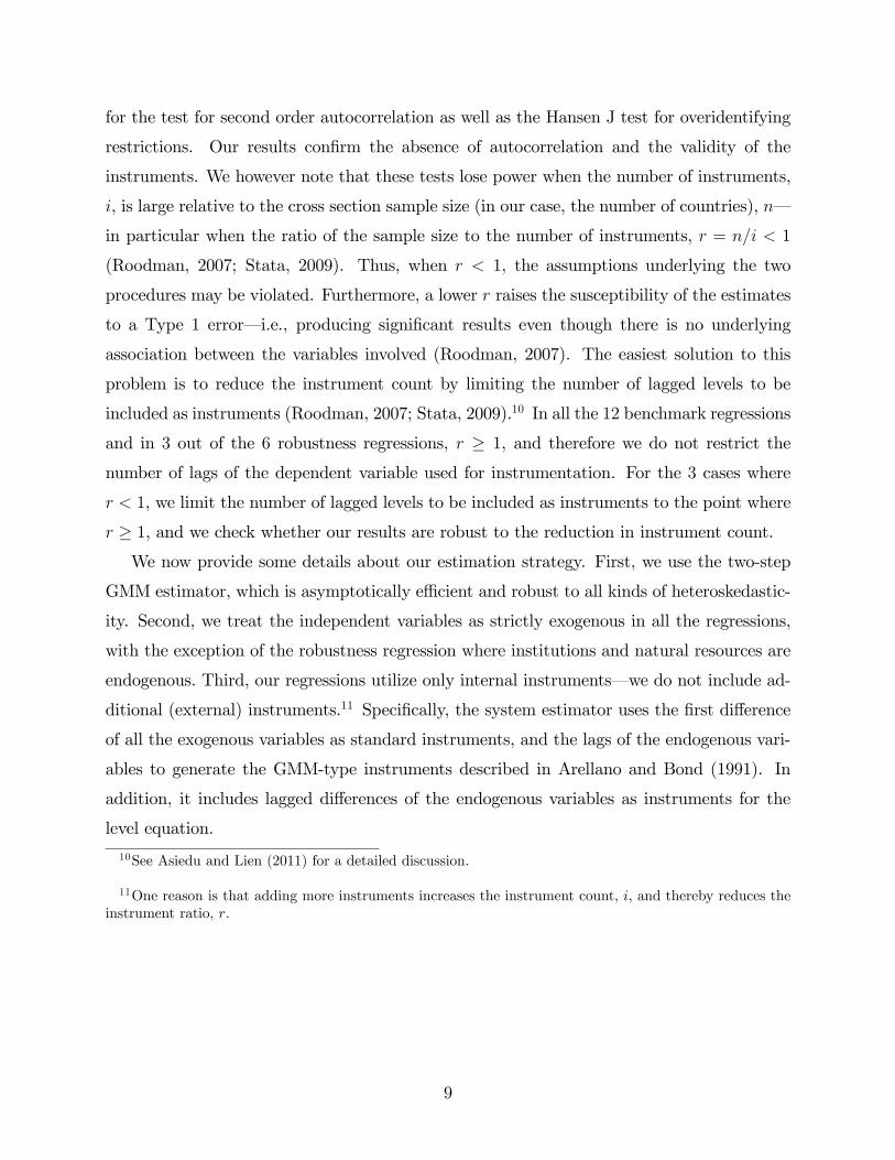
for the test for second order autocorrelation as well as the Hansen J test for overidentifying
restrictions. Our results confirm the absence of autocorrelation and the validity of the
instruments. We however note that these tests lose power when the number of instruments,
i, is large relative to the cross section sample size (in our case, the number of countries), n–
in particular when the ratio of the sample size to the number of instruments, r = n/i < 1
(Roodman, 2007; Stata, 2009). Thus, when r < 1, the assumptions underlying the two
procedures may be violated. Furthermore, a lower r raises the susceptibility of the estimates
to a Type 1 error–i.e., producing significant results even though there is no underlying
association between the variables involved (Roodman, 2007). The easiest solution to this
problem is to reduce the instrument count by limiting the number of lagged levels to be
included as instruments (Roodman, 2007; Stata, 2009).10 In all the 12 benchmark regressions
and in 3 out of the 6 robustness regressions, r ≥ 1, and therefore we do not restrict the
number of lags of the dependent variable used for instrumentation. For the 3 cases where
r < 1, we limit the number of lagged levels to be included as instruments to the point where
r ≥ 1, and we check whether our results are robust to the reduction in instrument count.
We now provide some details about our estimation strategy. First, we use the two-step
GMM estimator, which is asymptotically e¢cient and robust to all kinds of heteroskedastic-
ity. Second, we treat the independent variables as strictly exogenous in all the regressions,
with the exception of the robustness regression where institutions and natural resources are
endogenous. Third, our regressions utilize only internal instruments–we do not include ad-
ditional (external) instruments.11 Specifically, the system estimator uses the first di§erence
of all the exogenous variables as standard instruments, and the lags of the endogenous vari-
ables to generate the GMM-type instruments described in Arellano and Bond (1991). In
addition, it includes lagged di§erences of the endogenous variables as instruments for the
level equation.
10See Asiedu and Lien (2011) for a detailed discussion.
11One reason is that adding more instruments increases the instrument count, i, and thereby reduces theinstrument ratio, r.
9
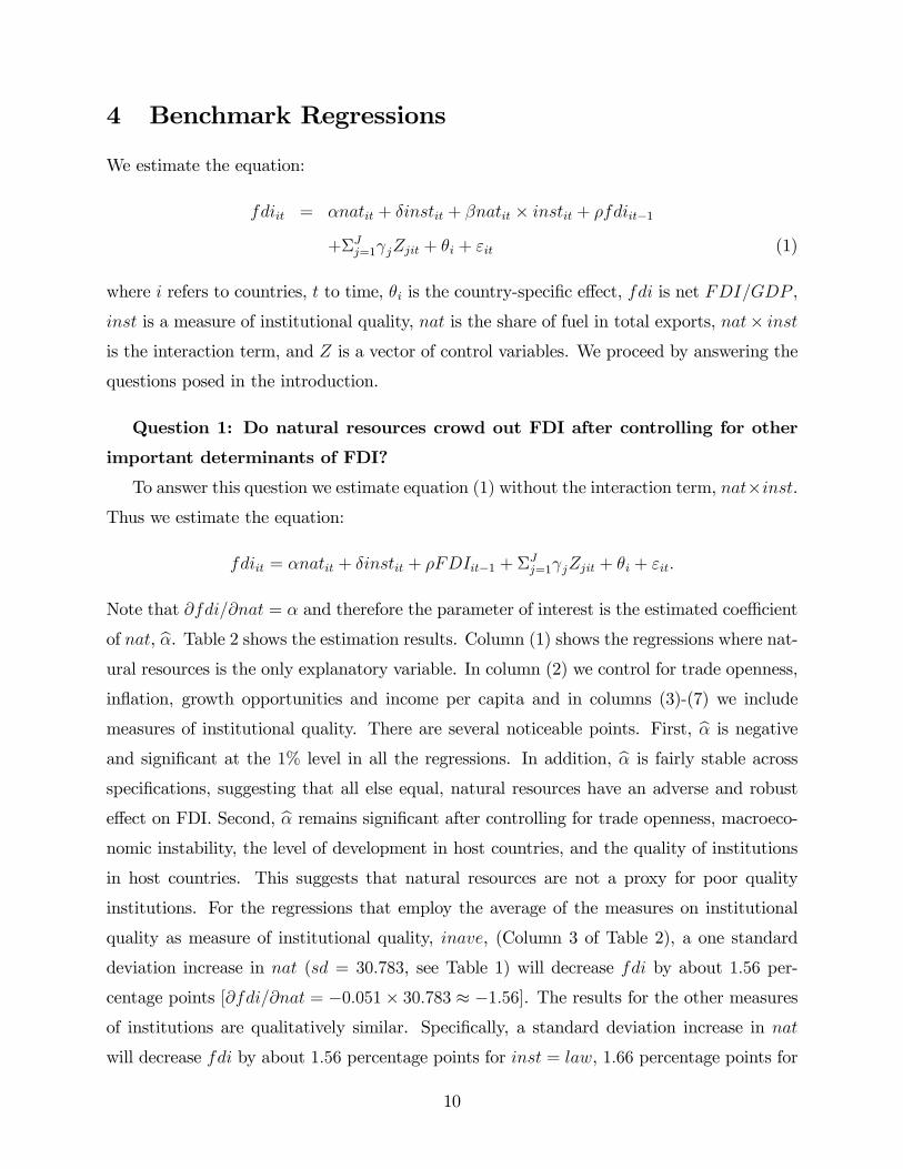
4 Benchmark Regressions
We estimate the equation:
fdiit = αnatit + δinstit + βnatit × instit + ρfdiit−1
+ΣJj=1γjZjit + θi + "it (1)
where i refers to countries, t to time, θi is the country-specific e§ect, fdi is net FDI/GDP ,
inst is a measure of institutional quality, nat is the share of fuel in total exports, nat× inst
is the interaction term, and Z is a vector of control variables. We proceed by answering the
questions posed in the introduction.
Question 1: Do natural resources crowd out FDI after controlling for other
important determinants of FDI?
To answer this question we estimate equation (1) without the interaction term, nat×inst.
Thus we estimate the equation:
fdiit = αnatit + δinstit + ρFDIit−1 + ΣJj=1γjZjit + θi + "it.
Note that @fdi/@nat = α and therefore the parameter of interest is the estimated coe¢cient
of nat, bα. Table 2 shows the estimation results. Column (1) shows the regressions where nat-ural resources is the only explanatory variable. In column (2) we control for trade openness,
inflation, growth opportunities and income per capita and in columns (3)-(7) we include
measures of institutional quality. There are several noticeable points. First, bα is negativeand significant at the 1% level in all the regressions. In addition, bα is fairly stable acrossspecifications, suggesting that all else equal, natural resources have an adverse and robust
e§ect on FDI. Second, bα remains significant after controlling for trade openness, macroeco-nomic instability, the level of development in host countries, and the quality of institutions
in host countries. This suggests that natural resources are not a proxy for poor quality
institutions. For the regressions that employ the average of the measures on institutional
quality as measure of institutional quality, inave, (Column 3 of Table 2), a one standard
deviation increase in nat (sd = 30.783, see Table 1) will decrease fdi by about 1.56 per-
centage points [@fdi/@nat = −0.051× 30.783 ≈ −1.56]. The results for the other measures
of institutions are qualitatively similar. Specifically, a standard deviation increase in nat
will decrease fdi by about 1.56 percentage points for inst = law, 1.66 percentage points for
10
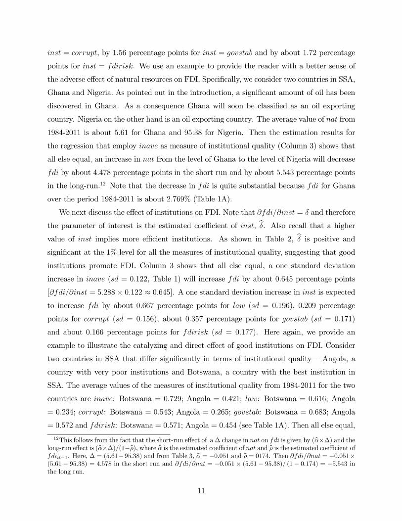
inst = corrupt, by 1.56 percentage points for inst = govstab and by about 1.72 percentage
points for inst = fdirisk. We use an example to provide the reader with a better sense of
the adverse e§ect of natural resources on FDI. Specifically, we consider two countries in SSA,
Ghana and Nigeria. As pointed out in the introduction, a significant amount of oil has been
discovered in Ghana. As a consequence Ghana will soon be classified as an oil exporting
country. Nigeria on the other hand is an oil exporting country. The average value of nat from
1984-2011 is about 5.61 for Ghana and 95.38 for Nigeria. Then the estimation results for
the regression that employ inave as measure of institutional quality (Column 3) shows that
all else equal, an increase in nat from the level of Ghana to the level of Nigeria will decrease
fdi by about 4.478 percentage points in the short run and by about 5.543 percentage points
in the long-run.12 Note that the decrease in fdi is quite substantial because fdi for Ghana
over the period 1984-2011 is about 2.769% (Table 1A).
We next discuss the e§ect of institutions on FDI. Note that @fdi/@inst = δ and therefore
the parameter of interest is the estimated coe¢cient of inst, bδ. Also recall that a highervalue of inst implies more e¢cient institutions. As shown in Table 2, bδ is positive andsignificant at the 1% level for all the measures of institutional quality, suggesting that good
institutions promote FDI. Column 3 shows that all else equal, a one standard deviation
increase in inave (sd = 0.122, Table 1) will increase fdi by about 0.645 percentage points
[@fdi/@inst = 5.288× 0.122 ≈ 0.645]. A one standard deviation increase in inst is expected
to increase fdi by about 0.667 percentage points for law (sd = 0.196), 0.209 percentage
points for corrupt (sd = 0.156), about 0.357 percentage points for govstab (sd = 0.171)
and about 0.166 percentage points for fdirisk (sd = 0.177). Here again, we provide an
example to illustrate the catalyzing and direct e§ect of good institutions on FDI. Consider
two countries in SSA that di§er significantly in terms of institutional quality– Angola, a
country with very poor institutions and Botswana, a country with the best institution in
SSA. The average values of the measures of institutional quality from 1984-2011 for the two
countries are inave: Botswana = 0.729; Angola = 0.421; law: Botswana = 0.616; Angola
= 0.234; corrupt: Botswana = 0.543; Angola = 0.265; govstab: Botswana = 0.683; Angola
= 0.572 and fdirisk: Botswana = 0.571; Angola = 0.454 (see Table 1A). Then all else equal,
12This follows from the fact that the short-run e§ect of a∆ change in nat on fdi is given by (bα×∆) and thelong-run e§ect is (bα×∆)/(1−bρ), where bα is the estimated coe¢cient of nat and bρ is the estimated coe¢cient offdiit−1. Here, ∆ = (5.61−95.38) and from Table 3, bα = −0.051 and bρ = 0174. Then @fdi/@nat = −0.051×(5.61 − 95.38) = 4.578 in the short run and @fdi/@nat = −0.051 × (5.61 − 95.38)/ (1− 0.174) = −5.543 inthe long run.
11
an improvement in institutional quality from the level of Angola to the level of Botswana
will increase fdi by about 1.629 percentage points for inave, 1.298 percentage points for law,
0.058, percentage points for corrupt, 0.827 percentage points for govstab and about 0.386
percentage points for fdirisk.
We now turn our attention to the other explanatory variables. The control variables
carry the expected signs and are all significant at the 1% level. The estimated coe¢cient
of lagged FDI is positive and significant, an indication that FDI is persistent. Indeed, this
provides justification for using the Blundell and Bond (1998) GMM estimator. The results
also show that the relationship between FDI and income per capita is non-linear: GDP per
capita has a positive impact on FDI only if income per capita exceeds a certain threshold.
Finally, consistent with many empirical studies on the determinants of FDI, we find that
GDP growth, openness to trade and lower inflation have a positive and significant e§ect on
FDI.
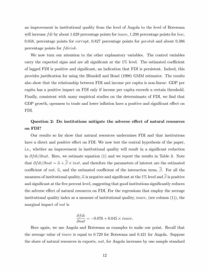
Question 2: Do institutions mitigate the adverse e§ect of natural resources
on FDI?
Our results so far show that natural resources undermines FDI and that institutions
have a direct and positive e§ect on FDI. We now test the central hypothesis of the paper,
i.e., whether an improvement in institutional quality will result in a significant reduction
in @fdi/@nat. Here, we estimate equation (1) and we report the results in Table 3. Note
that @fdi/@nat = bα + bβ × inst, and therefore the parameters of interest are the estimatedcoe¢cient of nat, bα, and the estimated coe¢cient of the interaction term, bβ. For all themeasures of institutional quality, bα is negative and significant at the 1% level and bβ is positiveand significant at the five percent level, suggesting that good institutions significantly reduces
the adverse e§ect of natural resources on FDI. For the regressions that employ the average
institutional quality index as a measure of institutional quality, inave, (see column (1)), the
marginal impact of nat is
@fdi
@nat= −0.076 + 0.045× inave.
Here again, we use Angola and Botswana as examples to make our point. Recall that
the average value of inave is equal to 0.729 for Botswana and 0.421 for Angola. Suppose
the share of natural resources in exports, nat, for Angola increases by one sample standard
12
deviation. Then for the regressions that employ inave as a measure of institutional quality
(Column 3), the increase in nat will decrease fdi in Angola by about 1.663 percentage points
[@fdi/@nat = (−0.073 + 0.045× 0.421)× 30.783 ≈ −1.663]. Now suppose Angola imple-
ments policies that lead to an improvement in its institutions, such that the value of inave in-
creases to the level of Botswana. Then, a one standard deviation increase in nat will decrease
fdi by only 1.237 percentage points [@fdi/@nat = (−0.073 + 0.045× 0.729)× 30.783 ≈ −1.237],
which is about 27 percent less than the expected decrease in fdi under the current level of in-
stitutional quality. An important to note is that the estimated coe¢cient of inst, bδ, remainssignificant suggesting that institutions have a direct and indirect impact on FDI.
Question 3: Can institutions completely neutralize the adverse e§ect of nat-
ural resources on FDI?
Having ascertained that institutions mitigate the adverse e§ect of natural resources on
FDI, a natural question that arises is this: can institutions eliminate the FDI-resource curse?
For our analysis, we are interested in determining the level of institutional quality that drives
@fdi/@nat to zero (i.e., bα+bβ×inst = 0). We proceed by evaluating @fdi/@nat at reasonablevalues of inst. Specifically we calculate the average value of the measures of institutional
quality over the period 1984-2011 for each of the countries in our sample, and we denote
it by inst. We then evaluate @fdi/@nat at the mean, 10th, 25th, 50th, 75th and the 90th
percentile of inst. Panel A of Table 4 shows the results for inave. The 10th, 25th, 50th,
75th and the 90th percentile of inave correspond to the average value of inave for Pakistan,
Venezuela, Mexico, South Africa and Latvia, respectively and the mean correspond to the
average value for Argentina. There are two notable points from Panel A. First, @fdi/@nat
decreases substantially as inave increases. The second notable point is that @fdi/@nat
remains negative and significant even when inave is quite high, as high as the 90th percentile
of inave . The other institutional measures produce similar results (see Panels B, C, D and
E). Note that these results suggest that although an improvement in institutional quality
mitigates the FDI-resource curse, it may not completely neutralize the negative e§ect of
natural resources on FDI. To confirm this conjecture, we compute the critical value of inst,
inst∗, defined as the level of inst at which @fdi/@nat = 0. Thus, inst∗ = −bα/bβ. The valueof inst∗ is about 1.68 for inave, 1.92 for law, 2.95 for corrupt, 8.18 for govstab and 3.52
for fdirisk. Note that the critical values are implausible because inst lies between 0 and 1.
Indeed, the highest values of the average measures of institutional quality for the countries
13
in our sample is 0.812 for inave , 0.918 for law, 0.767 for corr , 0.952 for govstab and 0.958
for fdirisk. Thus, the results confirm our conjecture, that overall, good institutions reduce
the FDI-resource curse, but cannot completely neutralize the resource curse.
5 Robustness Regressions
We run several regressions to test the robustness of our main results: that institutions miti-
gate the adverse e§ect of the natural resource curse on FDI. In order to keep the discussion
focused, we report the regressions which employ the measure of institutions that reflects the
overall institutional quality in host countries, inave. Furthermore, to conserve on space, we
report only the values of bα and bβ in Table 5 and Table 6. The preview of the outcome ofour robustness regressions is that our results are robust: bα is negative and significant atthe 1% level and bβ is positive and significant at least at the 5% level in all the regressions,
suggesting that institutions mitigate the adverse e§ect of natural resources on FDI. We now
provide a brief discussion of the robustness estimations.
(i) Sub-samples: We run regressions where we exclude countries in SSA. This exercise
is motivated by two reasons. Asiedu (2002) finds that the factors that drive FDI to SSA
are di§erent from the factors that drive FDI to other developing countries. Second, natural
resources dominates the exports of many of the countries in SSA. Thus, it is possible that our
results may change if SSA countries are excluded from the regressions. For this regression,
we limit the number of lagged variables used as instruments to ensure that r < 1. Clearly,
the results are robust: bα is positive and significant at the 1% level and bβ is negative andsignificant at the 5%.13
(ii) Alternative Measure of Institution: The measures of institutional quality em-
ployed in the benchmark regressions are from the same source, ICRG. We check whether
our results hold if we use data from a di§erent source. We use the rule of law variable from
Kau§man et al. (2012). Our results are robust to the alternative measures of institutional
quality: bα and bβ are significant at the 1% level.
(iii) Alternative Measure of Natural Resources: The resource curse literature
suggests that rents generated from natural resources play a significant role in explaining
13We do not run separate regressions for SSA because the instrument ratio, r = 0.76, is very low. Specifi-cally, n = 28 and i = 37. In addition, r remains less than one even after a reduction in the instrument count.As pointed out earlier, the results are not reliable when r < 1.
14
the natural resource curse.14 The measure of natural resources employed in the benchmark
regressions, oilex does not capture natural resource rents. As a robustness check we examine
whether the results hold when we use oil rents as a share of GDP, oilrent, as a measure of
natural resources in host countries. Here we limit the instrument count to ensure that r > 1.
As shown in Table 5, bα and bβ have the expected signs and are significant at the 1% level.
(iv) Internal Conflict and Political Instability: Several studies have found that
natural resource dependence generates political instability and internal conflict, in particu-
lar, civil wars (e.g., Collier and Hoeffler, 1998). We use the conflict index reported in Cross
National Time Series (CNTS) database as a measure of internal conflict in host countries.15
The measure, conflict, is the weighted average of the number of: assassinations, strikes,
guerrilla warfare, government crises, purges, riots, revolutions and anti-government demon-
strations. We did not include conflict in the benchmark regression because the estimated
coe¢cient of conflict is not significant. do not include a measure of political instability. Our
results are robust: bα and bβ have the correct signs and are significant at the 1% level.
(v) Alternative Measure for the Dependent Variable: We note that one could
use FDI per capita as a dependent variable to analyze the e§ect of natural resources on
FDI flows. Thus, we examine whether our results hold when we use FDI per capita as the
dependent variable. Column 1 of Table 6 shows that our results pass the robustness checks:
bα and bβ have the correct signs and are significant at the 1% level.
(vi) Endogeneity of Natural Resources and Institutional Quality: There is a
potential endogeneity problem associated with our measure of natural resources. Specifically,
it is possible that an unobserved variable may a§ect both FDI and exports. Since we measure
natural resources as a share of exports, it is possible that our estimates are biased. The
system estimator mitigates the endogeneity problem. However, in order to be thorough,
14Di§erent channels through which natural resources a§ect growth have been studied extensively, includingthe “voracity e§ect” induced by rent-seeking. The “voracity e§ect” is formalized by Lane and Tornell (1996)and Tornell and Lane (1999) . Di§erent interest groups, fight to capture a greater share of the rents fromnatural resources, and this induces a bad allocation of resources — public subsidies and other forms of transfersgrow more quickly than the increase in windfall income, lowering the e§ective rate of return to investment.Torvik (2002) argues that a greater amount of natural resources increase the number of entrepreneurs engagedin rent seeking and reduces the number of entrepreneurs running productive firms. Hodler (2006) findsnatural resources lower incomes in fractionalized countries but increase incomes in homogenous countriessince natural resources cause fighting activities between rivalling groups which in turn reduces productiveactivities and weakens property rights.15The data are produced by Databank International. For more details see
http://www.databanksinternational.com
15
we address this issue explicitly by specifying natural resources as an endogenous variable in
our regression. Note that if natural resource is endogenous, then the interaction between
institutional quality and natural resources is also endogenous. Thus here, we re-estimate
equation (1) where we specify oiex and oilex×inst as endogenous variables. We also take into
consideration the potential endogeneity of institutions, and consider a specification where
inst and oilex× inst are specified as endogenous variables. As expected, the introduction of
the endogenous variables increases the instrument count substantially, and as a consequence
r is low.16 We therefore curtail the number of instruments. As shown in Columns 2 and 3 of
Table 6, the results are robust: bα and bβ are significant at the 1% level and have the correct
signs.
(vii) Time and Region Fixed e§ects: We test whether our results hold when we take
into account time and region fixed e§ects. We did not include the regional and time dummy
variables in our main regressions because it lowers r. The results reported in Columns 4 and
5 of Table 6 show that the results are robust.
6 Implications of Results for SSA and Ghana
As pointed out in the introduction, the paper has important implications for SSA countries.
There are four reasons for this. First, there has been a significant increase in the exploration
and production of oil in the region. As a consequence more countries in the region will
soon be classified as natural resource exporting countries. Second, several studies have
shown that FDI is crucial for poverty reduction in SSA (Asiedu and Gyimah-Brempong,
2008). Third, although FDI to SSA has increased substantially since 2000, the investments
are concentrated in extractive industries. The fourth reason is that most of the countries
in SSA, in particular, natural resource exporting countries have weak institutions. It is
therefore important to analyze how the quality of institutions in the host country a§ect the
natural resources (increased oil production)-FDI relationship. In this section we provide data
to support these assertions and discuss the policy implications of our results for countries in
SSA. In addition we use Ghana as an example of an emerging resource exporting country to
highlight the implications of our results for countries that have recently discovered oil.
16For example the instrument count increases from 86 for the case where oilex is exogeneous to 215 whenoilex and oilex× inst are endogenous.
16

6.1 FDI, Oil Production and Institutions in SSA
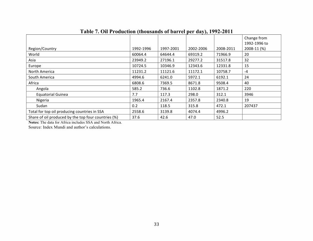
The production of crude oil in Africa has increased substantially since the 1990s. Table 7
shows the average daily production of crude oil for the world, the various geographical regions
and the top four oil exporting countries in SSA: Angola, Equatorial Guinea, Nigeria and
Sudan, from 1992 to 2011. There are several notable points in Table 7. First, oil production
grew faster in Africa than in the other regions. Over the period 1992-96 to 2008-11, oil
production in Africa increased by 40%. This compares with an increase of 32% for Asia,
24% for South America, 15% for Europe, and a decline of 4% for North America. Second,
the growth in production in Equatorial Guinea and Sudan was quite substantial: 3, 946% for
Equatorial Guinea and 207, 437% for Sudan. Third, a large share of the production in Africa
occurred in the top four oil exporting countries, with the share of production increasing
from about 38% to about 53%. Note that oil was discovered in Equatorial Guinea in 1990
and in Sudan in 1991, suggesting that the increase in oil production in SSA is driven by
new discoveries. This indeed underscores the point made earlier, that the rise in the global
demand for oil is being met by increased production of oil in SSA.
Figure 1 displays FDI flows to SSA from 1980-2011, and it shows that FDI to the region
has increased substantially since 2000. From 2000-2011, net FDI inflows to the region in-
creased by about 368% in real terms–from $7, 598 million in 2000 to $35, 596 million in 2011
(WDI, 2013). Indeed, from 1990-1999 to 2000-2009, average annual FDI to SSA grew faster
than FDI to non-SSA developing countries (excluding China): FDI growth for SSA was
about 1.6 times the growth in non-SSA developing countries; 4.5 times the growth in East
Asia and Pacific, and about 4 times the growth in Latin America (WDI, 2013). However, the
investments are concentrated in oil-exporting countries. For example in 2009, about 43% of
FDI flows to SSA went to the top four oil-exporting countries (Angola, Equatorial Guinea,
Nigeria and Sudan) and the share is higher when FDI to South Africa is excluded—the share
increases to 51%. Note that this implies that the remaining 43 countries in the region re-
ceived only 49% of the investment. The conjecture is supported by Figure 2, which shows a
graph of FDI flows and the share of oil in total exports for 21 countries in SSA, averaged from
2000-2009. The graph shows a positive correlation between FDI and oil export intensity. An
ordinary least square regression of ln(FDI) on oil export intensity yielded a coe¢cient of
0.033, with a robust p-value 0.007 and R2 = 0.26. This implies that all else equal, a one
percentage point increase in oil export intensity will raise FDI by about 3.3%.is supported.
17

Thus, one can infer from the data that the recent increase in FDI to SSA is mainly in the
oil industry.
Table 8 shows the data for two measures of institutional quality, corruption and the e§ec-
tiveness of the rule of law, for SSA countries and developing countries outside SSA. We also
report the data for the eight top oil exporting countries in SSA: Angola, Cameroon, Chad,
Congo Republic, Equatorial Guinea, Gabon, Nigeria, and Sudan. The data are averaged
from 2000-2009 and they range from zero to one. A higher number implies a higher level
of corruption and a more e§ective legal system. Table 8 shows that the average corruption
index for SSA is higher than the index for non-SSA countries, and the average index for the
eight oil exporting countries is higher than the index for SSA. This suggests that corruption
is more prevalent in SSA countries than in non-SSA countries, and that oil exporting coun-
tries are more corrupt than non-oil exporting countries. The rule of law index is higher for
non-SSA countries than SSA countries, and lower for oil exporting countries. Thus the data
suggests that overall SSA has weaker institutions than other developing countries, and oil
exporting countries in SSA have worse institutions than non-oil exporting countries in the
region.
6.2 FDI, Oil Production and Institutions in Ghana
Oil was discovered in Ghana in 2007 and production began in 2010.17 Production has in-
creased significantly since 2010. Specifically, production in 2010, 2011 and 2012 was 7.19
million bpd, 72.58 million bpd and 2000 million bpd (Index Mundi, 2013). Thus, oil produc-
tion in Ghana increased by 175% within a year, from 2011-2012. The surge in oil production
is reflected in the increase in the share of oil in exports from 2009 to 2011. Oil as a share of
exports increased from about 4% in 2009 to 54% in 2012 (WDI, 2013). If this trend continues,
then it is likely that very soon, Ghana will be classified as an oil exporting country.
Figure 3 shows FDI flows to Ghana from 1980 to 2011. FDI to Ghana has increased
substantially since 2005. From 2005 to 2011, FDI increased by about 1, 834% in real terms,
from $140 million to $2, 7778 million. Table 9 shows investments by firms in the extractive
industries from 1991-2010. As pointed out earlier, foreign firms dominate the extractive
industry, hence the data may be interpreted as FDI in extractive industries. The data shows
17See GNPC (2011) for a discussion about the history of oil and gas exploration in Ghana.
18
that FDI in extractive industries has increased significantly since 1991. Over the periods
1991-1995, 1996-2000, 2001-2005 and 2006-2010, the average annual investment increased
from $385 million to $470 million, to $515 million to $631 million (constant 2005 dollars),
respectively. In addition, over the periods 2001-2005 to 2006-2010, total investments in the
extractive industry increased by about 23%.
We now discuss how institutional quality in Ghana has evolved over time. Figure 4 shows
the trend for corruption and Figure 5 shows the trend for law and order from 1987-2011.
The graphs show that Ghana has weak institutions and the quality of institutions has gotten
worse over time. For example, the corruption index increased from 0.48 in 1987-1991 to
about 0.7 in 2007-2011, and the rule of law index declined from 0.49 to 0.39 over the same
period.
6.3 Discussion—Policy Implications
Our discussion so far suggests that a continual increase in oil production in SSA will expose
more countries in the region to the FDI-natural resource curse. Another important point is
that good institutions can mitigate the adverse e§ect of natural resources on FDI. However,
SSA countries have weak institutions, suggesting that the curse, if it occurs will be more
severe in African countries. We end the section by discussing the importance of FDI to SSA
and highlighting the potential e§ect of the FDI-natural resource curse on poverty reduction
and economic growth. We also discuss policies that may mitigate the “curse”.
The importance of FDI to SSA is well articulated in the United Nations Millennium
Declaration Goal (MDG) document, adopted in September 2000, that notes that
“We [the United Nations General Assembly] resolve to halve, by the year 2015,
the proportion of the world’s people whose income is less than one dollar a day.
We also resolve to take special measures to address the challenges of poverty
eradication and sustainable development in Africa, including debt cancellation,
improved market access, enhanced O¢cial Development Assistance and increased
flows of Foreign Direct Investment,... ”
It is important to note that the impact of FDI on host economies depends on the type
of FDI that the country receives (Asiedu, 2004; Axarloglou and Pournarakis, 2007). Thus
an important issue that comes to bear is whether the recent increase in extractive industry
19
FDI will enhance economic growth and reduce poverty in SSA countries. We assert that
employment by MNCs is one of the most e§ective ways by which FDI can facilitate poverty
reduction and economic growth in host countries. MNC employment increases domestic
employment, boosts domestic wages, enhances the productivity of the labor force and it
fosters the transfer of technology between foreign and domestic firms (Asiedu, 2004). How-
ever, extractive industry FDI generates very limited local employment. This point is noted
in UNCTAD (2007: 92): “mineral extraction is primarily an export-oriented activity, with
significant revenue creation, but limited opportunities for employment creation and local
linkages”. The employment e§ects of FDI are important to SSA, because in most African
countries unemployment is prevalent. High unemployment rate countries in SSA include
South Africa, 23%; Kenya, 40%; Senegal, 48% and Zambia, 50% (CIA, 2011). In addition to
expanding domestic employment, MNC employment boosts wages in host countries. MNCs
pay higher wages than domestic firms and the presence of multinationals generates wage
spillover: wages tend to be higher in industries and in provinces that have a greater foreign
presence (Asiedu, 2004; Lipsey and Sjoholm, 2001). This is important because wages are low
in SSA. For example, about 46% of the workers in South Africa (one of the richest countries
in the region), earn less than the living wage (Fields, 2000). Thus, for countries such as
South Africa, the contribution of FDI to employment is crucial. Indeed, foreign a¢liates
accounted for about 23% of employment in South Africa in 1999 (UNCTAD, 2002).
We employ data from US MNCs to show that FDI in manufacturing generates more
jobs than FDI in extractive industries in Africa. Specifically, we compare the employment
e§ects of FDI in manufacturing and extractive industries. For each industry, we compute
the number of employees per $1 million stock of FDI of a¢liates of US MNCs abroad,
and we use this measure as a proxy for the elasticity of job creation. Table 10 shows the
employment elasticity data for the World and the various regions. A higher elasticity implies
FDI generates more jobs. We also report the elasticity ratio, which we define as the ratio of
the elasticity for manufacturing to the elasticity for mining. There are three notable points.
First, the elasticity ratios are greater than one, suggesting that in all the regions, an equal
investment in manufacturing and mining will produce more jobs in manufacturing than in
mining. For example the elasticity ratio for Africa is 17, which means that for the same level
of investment, the number of jobs created in manufacturing will be equal to 17 times the
number of jobs created in mining. Second, Africa has the highest elasticity ratio, implying
20
that the relative benefit (in terms of job creation) of receiving FDI in manufacturing versus
FDI in mining is higher for Africa than the other regions. Third, Africa has the highest
employment elasticity in manufacturing. A $1 million investment in manufacturing will
create about 34 jobs in SSA–this compares with 21 in Latin America, 15 in Asia and about
10 in Europe and the Middle East. This implies that in terms of employment creation,
manufacturing FDI is more “productive” in Africa than in other regions.
Thus, the challenge facing countries in SSA, in particular, oil-exporting countries in the
region, such as Ghana, is to find ways to avoid the FDI resource curse and attract FDI in
non-extractive industries. In analyzing this issue, it is important to note that non-extractive
industry FDI is sensitive to the conditions in host economies, in particular, the size of the
local market, quality of physical infrastructure, the productivity of the labor force, openness
to trade, FDI policy and the quality of institutions. Another relevant point is that non-
extractive industry FDI is more footloose than FDI in extractive industry. This implies that
countries in SSA need to compete with developing countries outside SSA in order to attract
non-extractive FDI.
Three policy recommendations emerge from our discussion. First, countries in the region
need to improve their institutions and this is particularly relevant for resource-exporting
countries. Second, countries in SSA need to boost investments in physical infrastructure
and education. Here, oil-exporting countries have an advantage, in that they can use some
of the rents that accrue from oil production to finance these investments. The results also
suggest that regional economic cooperation may facilitate FDI to SSA (Elbadawi and Mwega,
1997).18 One reason is that regionalism expands the size of the market, and therefore makes
the region more attractive for FDI. The importance of large markets for FDI in Africa is
documented in several surveys. For example, “narrow and missing markets” was cited as
the main factor preventing French companies from investing in African countries (Arias-
Chamberline, 2002).19 The market size advantage of regionalism is particularly important
for Africa because countries in the region are small, in terms of population and income.
For example, 15 out of the 48 countries in SSA have a population of less than two million
18An example of a successful regional bloc in SSA is the Southern African Development Community(SADC). Countries in the SADC include Angola, Botswana, Congo Dem Rep, Lesotho, Malawi, Mauritius,Mozambique, Namibia, Seychelles, South Africa, Swaziland, Tanzania, Zambia and Zimbabwe. Elbadawi andMwega (1997) find evidence that after controlling for relevant country conditions, countries in the SADCregion receive more FDI than other countries in Africa.19The discusssion on regionalism draws from Asiedu (2006).
21

and about half of the countries have a population of less than six million. With regards to
income, about half of the countries have a GDP of less than $3 billion. Indeed, the total
GDP of SSA in 2009 was $956 billion, which was about equal to the GDP of Mexico and
about 61% the GDP of Brazil (WDI, 2011). Furthermore, SSA’s GDP falls to about $498
billion (i.e., about 30% the GDP of Brazil and about 57% the GDP of Mexico) when Nigeria
and South Africa are excluded. 20 Thus, due to the small size of African countries (both in
terms of income and population), a large number of countries will have to be included in the
regional bloc in order to achieve a market size that will be large enough to be attractive to
foreign investors.
Finally, we note that an increase in FDI, even in the manufacturing industry, does not
necessarily translate into higher economic growth. Specifically, several studies have found
that FDI enhances growth only under certain conditions — when the host country’s education
exceeds a certain threshold (Borensztein et al., 1998); when domestic and foreign capital are
complements (de Mello, 1999); when the country has achieved a certain level of income
(Blomstrom et al., 1994); when the country is open (Balasubramanyam et al., 1996) and
when the host country has a well-developed financial sector (Alfaro et al., 2004). Therefore
for countries in the region, reaping the benefits that accrue from FDI may be more di¢cult
than attracting FDI. However, there is room for optimism. The policies that promote FDI
also have a direct impact on long-term economic growth. As a consequence, African countries
cannot go wrong implementing such policies.
7 Conclusion
This paper has empirically examined the link between FDI, natural resources and institu-
tions. We find that natural resources have a negative e§ect on FDI and good institutions
mitigate the adverse e§ect of natural resources on FDI, but institutions cannot neutralize the
adverse e§ect. We also find that good institutions have a direct e§ect on FDI. With regard
to policy, our results suggest that an improvement in institutional quality will be beneficial
to countries, but more beneficial to natural resource rich economies. This recommendation
is particularly relevant for countries in Sub-Saharan Africa, since many of the countries in
the region are rich in natural resources, have weak institutions and are in dire need of FDI.
20In 2009, the share of SSA’s GDP from Nigeria and South Africa, was 18 percent and 30 percent,respectively.
22
References
[1] Acemoglu, Daron, Simon Johnson, James A. Robinson and Pierre Yared (2008), “In-
come and Democracy,” American Economic Review 98(3), 808—842.
[2] Alfaro, L., A. Chanda, S. Kalemli-Ozcan, and S. Sayek (2004), “FDI and Economic
Growth: the Role of Local Financial Markets,” Journal of International Economics 64,
89—112.
[3] Arias-Chamberline (2002), “Constraints of FDI to the ACP,” mimeo.
[4] Arellano, Manuel and Olympia Bover, 1995, “Another Look at the Instrumental Variable
Estimation of Error Component Models,” Journal of Econometrics 68, 29—51.
[5] Arellano, Manuel and Stephen Bond, 1991, “Some Tests of Specification for Panel Data:
Monte Carlo Evidence and an Application to Employment Equations,” Review of Eco-
nomic Studies 58, 277—297.
[6] Arezki, Rabah, and Frederick van der Ploeg, 2007, “Can the Natural Resource Curse
Be Turned Into a Blessing? The Role of Trade Policies and Institutions,” IMF Working
Paper 07/55.
[7] Asiedu, Elizabeth, 2002, “On the Determinants of Foreign Direct Investment to Devel-
oping Countries: Is Africa Di§erent?,” World Development 30(1), 107—119.
[8] Asiedu, Elizabeth, and Donald Lien, 2011, “Democracy, Foreign Direct Investment and
Natural Resources,” Journal of International Economics 84, 99—111.
[9] Asiedu, Elizabeth and Donald Lien, 2003, “Capital Controls and Foreign Direct Invest-
ment,” World Development 32(3), 479—490.
[10] Asiedu, Elizabeth and Kwabena Gyimah-Brempong, 2008, “The Impact of Trade and
Investment Liberalization on Foreign Direct Investment, Wages and Employment in
Sub-Saharan Africa,” African Development Review 20(1), 49—66.
[11] Axarloglou, Koutas, and Mike Pournarakis (2007). “Do All Foreign Direct Investment
Inflows Benefit the Local Economy?” The World Economy 30(3), 424—445.
23
[12] Balasubramanyam, V. N., Salisu, M. and Sapsford, D. (1996). “FDI and growth in EP
and IS countries,” The Economic Journal 106, 92—105.
[13] Blundell, Richard and Stephen Roy Bond, 1998, “Initial Conditions and Moment Re-
strictions in Dynamic Panel Data Models,” Journal of Econometrics 87, 115—144.
[14] CIA (2011). TheWorld Factbook. https://www.cia.gov/library/publications/the-world-
factbook/
[15] Collier, Paul and Anke Hoeffler, 1998, “On Economic Causes of Civil War,” Oxford
Economic Papers 50(4), 563—573.
[16] Collier, Paul and Anke Hoeffler, 2009, “Testing the Neocon Agenda: Democracy in
Resource-rich Societies,” European Economic Review 53, 293—308.
[17] de Mello, Luiz Jr (1999). “Foreign Direct Investment-Led Growth: Evidence from Time
Series and Panel Data,” Oxford Economic Papers 51(1), 133—151.
[18] Elbadawi, Ibrahim and Francis Mwega (1997). “Regional Integration, Trade, and For-
eign Direct Investment in Sub-Saharan Africa,” in Zubair Iqbal and Moshin Khan (eds.),
Trade Reform and Regional Integration in Africa, International Monetary Fund, Wash-
ington, D.C.
[19] EIA (2013). Energy Information Administration. http://www.eia.doe.gov/
[20] Fields, Gary (2000). “The Employment Problem in South Africa,” mimeo.
[21] Gylfason T. and G. Zoega (2006). “Natural Resources and Economic Growth: The Role
of Investment,” The World Economy 29, 1091—1115
[22] GNPC (2011). “Summaries of Recent Activities in the Oil and Gas Sector,” mimeo.
[23] Hayakawa, Kazuhiko, 2007, “Small Sample Bias Properties of the System GMM Esti-
mator in Dynamic Panel Data Models,” Economics Letters 95(1), 32—38.
[24] Hodler, Roland, 2006, “The Curse of Natural Resources in Fractionalized Countries,”
European Economic Review 50, 1367—1386.
[25] Index Mundi, 2013. http://www.indexmundi.com
24
[26] Kau§man, Daniel, Kraay, Aart and Massimo Mastruzzi, 2012, “The Worldwide Gover-
nance Indicators (WGI) project.”
[27] Lipsey, Robert E. and Sjoholm, Fredrik (2001). “Foreign Direct Investment andWages in
Indonesian Manufacturing”. NBERWorking Paper 8299. Cambridge, MA: National Bu-
reau of Economic Research. Gasganaga, Victor, Nugent, Je§erey, and Bistra Pashamova,
1998, “Host Country Reforms and FDI Inflows: How Much Di§erence Do They Make?”
World Development 26(7), 1299—1314.
[28] Poelhekke, Stecen, and Frederick van der Ploeg, 2010, “Do Natural Resources Attract
FDI? Evidence from Non-Stationary Sector-Level Data,” CEPR Discussion Paper 8079.
[29] Roodman, David, 2007, “A Short Note on the Theme of Too Many Instruments,” Center
for Global Development Working Paper 125.
[30] Sachs, Je§rey D., and Andrew M. Warner, 1995, “Natural Resource Abundance and
Economic Growth,” NBER Working Paper Series, 5398, 1—47.
[31] Stata, 2009. Stata Longitudinal Data/Panel Data Reference Manual, Stata Press, Col-
lege Station, TX: Stata Corp LP.
[32] Tornell, Aaron, and Philip Lane, 1999, “The Voracity E§ect,” The American Economic
Review 89(1), 22—46.
[33] UNCTAD (2002). World Investment Report, Transnational Corporations and Export
Competitiveness, United Nations, New York and Geneva.
[34] UNCTAD (2007). World Investment Report: Transnational Corporations, Extractive
Industries and Development. Geneva: UNCTAD.
[35] UNCTAD (2008). World Investment Report: Transnational Corporations and the In-
frastructure Challenge. Geneva: UNCTAD.
[36] UNCTAD (2009) World Investment Prospect Survey. Geneva: UNCTAD.
[37] WDI (2013). World Development Indicators. CD-Rom. Washington, DC: World Bank.
[38] Wei, Shang-Jin, 2000, “Local Corruption and Global Capital Flows,” Brookings Papers
on Economic Activity 2, 303—346.
25

[39] Wheeler, David, and Ashoka Mody, 1992, “International Investment Location Decisions:
The Case of U.S. firms,” Journal of International Economics 33, 57—76.
26

Table 1: Summary Statistics
Variables Mean Std. Dev. Min Max
Law and Order (ICRG) 0.547 0.196 0.046 1
Government Stability 0.647 0.171 0.132 1
FDI Risk 0.593 0..177 0.083 1
Corruption 0.429 0.156 0.000 1
Law and Order (Kau§man) 0.43 0.137 0.143 0.841
Overall Institutional Quality 0.554 0.122 0.159 0.894
Fuel/Exports (%) 21.615 30.783 0.000 98.786
Oil rents/GDP (%) 6.986 11.934 0.000 58.798
FDI/GDP (%) 2.921 3.964 -28.916 32.933
FDI per capita 1.718 6.954 -5.851 107.401
Trade/GDP (%) 78.730 53.856 12.227 434.185
GDP growth 6.812 2.215 0.000 10.000
Ln (GDP per capita) 7.366 1.250 4.764 10.476
Inflation 0.473 3.703 -0.084 77.797
Domestic Conflict 0.956 1.593 0.000 11.583
27
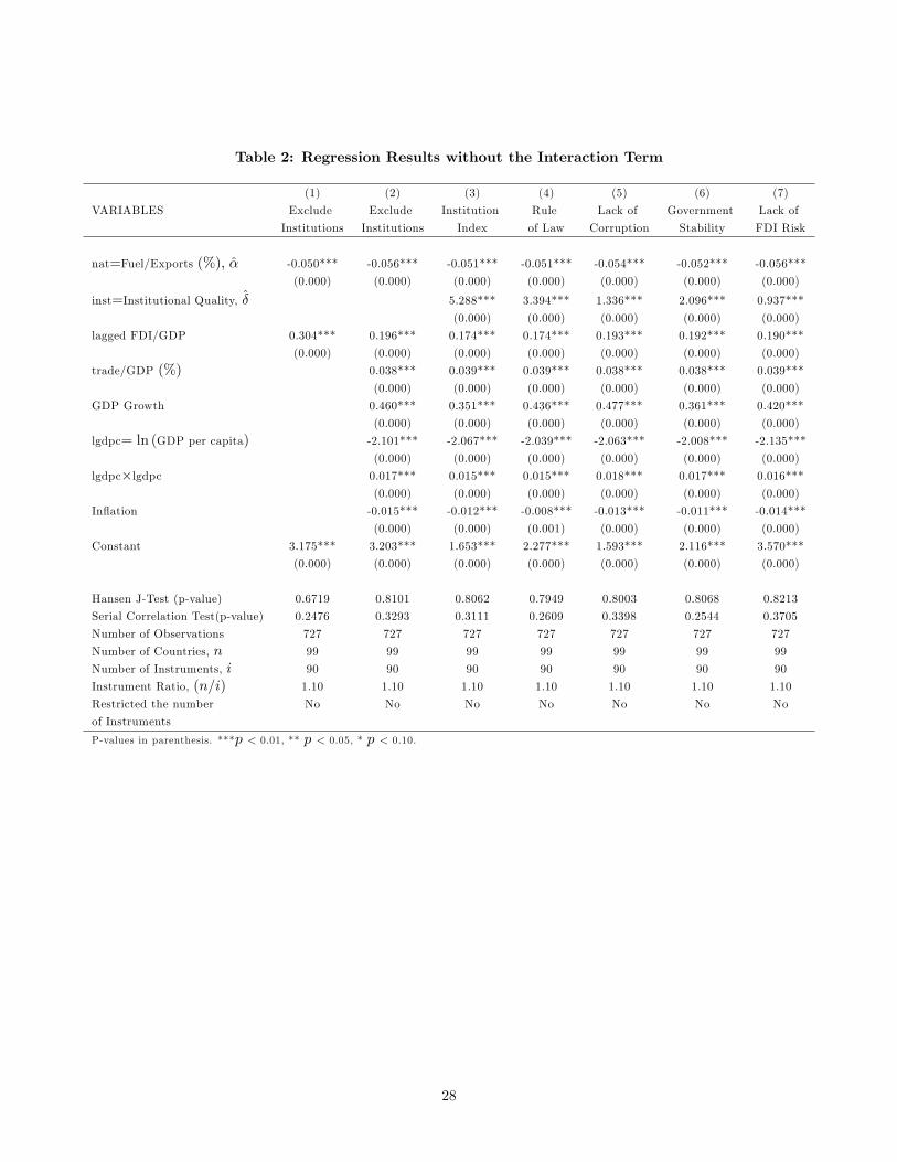
Table 2: Regression Results without the Interaction Term
(1) (2) (3) (4) (5) (6) (7)
VARIABLES Exclude Exclude Institution Rule Lack of Government Lack of
Institutions Institutions Index of Law Corruption Stability FDI Risk
nat=Fuel/Exports (%), α̂ -0.050*** -0.056*** -0.051*** -0.051*** -0.054*** -0.052*** -0.056***
(0.000) (0.000) (0.000) (0.000) (0.000) (0.000) (0.000)
inst=Institutional Quality, δ̂ 5.288*** 3.394*** 1.336*** 2.096*** 0.937***
(0.000) (0.000) (0.000) (0.000) (0.000)
lagged FDI/GDP 0.304*** 0.196*** 0.174*** 0.174*** 0.193*** 0.192*** 0.190***
(0.000) (0.000) (0.000) (0.000) (0.000) (0.000) (0.000)
trade/GDP (%) 0.038*** 0.039*** 0.039*** 0.038*** 0.038*** 0.039***
(0.000) (0.000) (0.000) (0.000) (0.000) (0.000)
GDP Growth 0.460*** 0.351*** 0.436*** 0.477*** 0.361*** 0.420***
(0.000) (0.000) (0.000) (0.000) (0.000) (0.000)
lgdpc= ln (GDP per capita) -2.101*** -2.067*** -2.039*** -2.063*** -2.008*** -2.135***
(0.000) (0.000) (0.000) (0.000) (0.000) (0.000)
lgdpc×lgdpc 0.017*** 0.015*** 0.015*** 0.018*** 0.017*** 0.016***
(0.000) (0.000) (0.000) (0.000) (0.000) (0.000)
Inflation -0.015*** -0.012*** -0.008*** -0.013*** -0.011*** -0.014***
(0.000) (0.000) (0.001) (0.000) (0.000) (0.000)
Constant 3.175*** 3.203*** 1.653*** 2.277*** 1.593*** 2.116*** 3.570***
(0.000) (0.000) (0.000) (0.000) (0.000) (0.000) (0.000)
Hansen J-Test (p-value) 0.6719 0.8101 0.8062 0.7949 0.8003 0.8068 0.8213
Serial Correlation Test(p-value) 0.2476 0.3293 0.3111 0.2609 0.3398 0.2544 0.3705
Number of Observations 727 727 727 727 727 727 727
Number of Countries, n 99 99 99 99 99 99 99
Number of Instruments, i 90 90 90 90 90 90 90
Instrument Ratio, (n/i) 1.10 1.10 1.10 1.10 1.10 1.10 1.10
Restricted the number No No No No No No No
of Instruments
P-values in parenthesis. ***p < 0.01, ** p < 0.05, * p < 0.10.
28
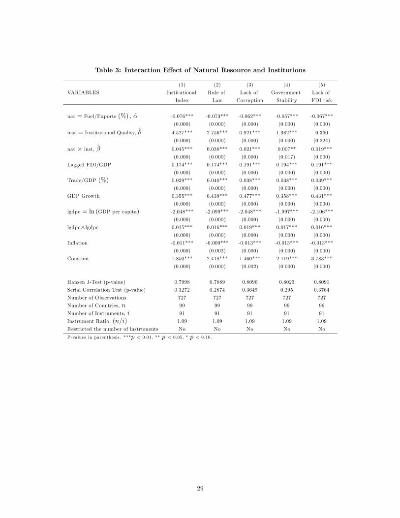
Table 3: Interaction E§ect of Natural Resource and Institutions
(1) (2) (3) (4) (5)
VARIABLES Institutional Rule of Lack of Government Lack of
Index Law Corruption Stability FDI risk
nat = Fuel/Exports (%) , α̂ -0.076*** -0.073*** -0.062*** -0.057*** -0.067***
(0.000) (0.000) (0.000) (0.000) (0.000)
inst = Institutional Quality, δ̂ 4.527*** 2.756*** 0.921*** 1.982*** 0.360
(0.000) (0.000) (0.000) (0.000) (0.224)
nat × inst, β̂ 0.045*** 0.038*** 0.021*** 0.007** 0.019***
(0.000) (0.000) (0.000) (0.017) (0.000)
Lagged FDI/GDP 0.174*** 0.174*** 0.191*** 0.194*** 0.191***
(0.000) (0.000) (0.000) (0.000) (0.000)
Trade/GDP (%) 0.039*** 0.040*** 0.038*** 0.038*** 0.039***
(0.000) (0.000) (0.000) (0.000) (0.000)
GDP Growth 0.355*** 0.439*** 0.477*** 0.358*** 0.431***
(0.000) (0.000) (0.000) (0.000) (0.000)
lgdpc = ln (GDP per capita) -2.048*** -2.099*** -2.048*** -1.997*** -2.106***
(0.000) (0.000) (0.000) (0.000) (0.000)
lgdpc×lgdpc 0.015*** 0.016*** 0.019*** 0.017*** 0.016***
(0.000) (0.000) (0.000) (0.000) (0.000)
Inflation -0.011*** -0.009*** -0.013*** -0.013*** -0.013***
(0.000) (0.002) (0.000) (0.000) (0.000)
Constant 1.850*** 2.418*** 1.460*** 2.119*** 3.783***
(0.000) (0.000) (0.002) (0.000) (0.000)
Hansen J-Test (p-value) 0.7998 0.7889 0.8096 0.8023 0.8091
Serial Correlation Test (p-value) 0.3272 0.2874 0.3649 0.295 0.3764
Number of Observations 727 727 727 727 727
Number of Countries, n 99 99 99 99 99
Number of Instruments, i 91 91 91 91 91
Instrument Ratio, (n/i) 1.09 1.09 1.09 1.09 1.09
Restricted the number of instruments No No No No No
P-values in parenthesis. ***p < 0.01, ** p < 0.05, * p < 0.10.
29

Table 4: @fdi/@inst = α̂+ β̂inst, evaluated at di§erent values of institutions
Panel A: Average Institutional Quality Panel D: Lack of FDI riskPercentile Corresponding Value Measure of Percentile Corresponding Value Measure of
Country Institutions Country Institutions
10 Pakistan 0.488 -0.0544 10 Syria 0.44 -0.059
(0.000) (0.000)
25 Venezuela 0.485 -0.0545 25 Brazil 0.584 -0.0575
(0.000) (0.000)
50 Mexico 0.553 -0.0515 50 Albania 0.586 -0.0563
(0.000) (0.000)
Mean Argentina 0.564 -0.0510 Mean Russia 0.602 -0.056
(0.000) (0.000)
75 South Africa 0.614 -0.0488 75 Mexico 0.676 -0.0555
(0.000) (0.000)
90 Hong Kong 0.730 -0.0468 90 Singapore 0.804 -0.0522
(0.000) (0.000)
Panel B: Corruption Panel E: Rule of LawPercentile Corresponding Value Measure of Percentile Corresponding Value Measure of
Country Institution Country Institution
10 Armenia 0.277 -0.05565 10 Nigeria 0.344 -0.0597
(0.000) (0.000)
25 Phillipines 0.335 -0.0544 25 South Africa 0.427 -0.0565
(0.000) (0.000)
50 Cote D’Ivoire 0.418 -0.0526 50 India 0.552 -0.0518
(0.000) (0.000)
Mean Syria 0.42 -0.0526 Mean Argentina 0.563 -0.0513
(0.000) (0.000)
75 Dominican Republic 0.472 -0.0515 75 Malaysia 0.671 -0.0472
(0.000) (0.000)
90 Botswana 0.543 -0.05 90 Hong Kong 0.807 -0.042
(0.000) (0.000)
Panel C: Government StabilityPercentile Corresponding Value Measure of
Country Institution
10 Honduras 0.545 -0.0534
(0.000)
25 Panama 0.575 -0.0532
(0.000)
50 Lithuania 0.661 -0.0525
(0.000)
Mean Albania 0.668 -0.0525
(0.000)
75 Armenia 0.719 -0.0521
(0.000)
90 Hong Kong 0.804 -0.0514
(0.000)
30

Table 5: Robustness Regressions
(1) (2) (3) (4)
VARIABLES Exclude Alternative Alternative Control for
SSA measure of measure of Political
countries institutions Nat, oil rents Instability
nat = Fuel/Exports (%) , α̂ -0.097*** -0.160*** -0.195*** -0.072***
(0.000) (0.000) (0.000) (0.000)
inst = Institutional Quality, δ̂ 3.016** -0.612 1.520*** 4.561***
(0.022) (0.725) (0.009) (0.000)
nat × inst, β̂ 0.050** 0.244*** 0.154*** 0.039***
(0.044) (0.000) (0.000) (0.000)
Hansen J-Test (p-value) 0.0501 0.1995 0.1746 0.2773
Serial Correlation Test (p-value) 0.7621 0.6589 0.8662 0.7879
Number of Observations 547 512 754 723
Number of Countries, n 71 97 90 98
Number of Instruments, i 37 65 63 92
Instrument ratio, (n/i) 1.919 1.492 1.429 1.065
Restricted the number of instruments Yes No Yes No
P-values in parenthesis. ***p < 0.01, ** p < 0.05, * p < 0.10.
31
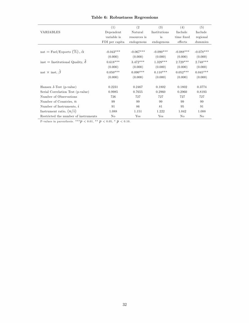
Table 6: Robustness Regressions
(1) (2 (3) (4) (5)
VARIABLES Dependent Natural Institutions Include Include
variable is resources is is time fixed regional
FDI per capita endogenous endogenous e§ects dummies
nat = Fuel/Exports (%) , α̂ -0.043*** -0.067*** -0.090*** -0.088*** -0.078***
(0.000) (0.000) (0.000) (0.000) (0.000)
inst = Institutional Quality, δ̂ 0.618*** 3.472*** 1.329*** 2.729*** 2.748***
(0.000) (0.000) (0.000) (0.000) (0.000)
nat × inst, β̂ 0.050*** 0.090*** 0.110*** 0.052*** 0.045***
(0.000) (0.000) (0.000) (0.000) (0.000)
Hansen J-Test (p-value) 0.2231 0.2467 0.1802 0.1802 0.3774
Serial Correlation Test (p-value) 0.9985 0.7655 0.2960 0.2960 0.8193
Number of Observations 726 727 727 727 727
Number of Countries, n 99 99 99 99 99
Number of Instruments, i 91 86 81 95 91
Instrument ratio, (n/i) 1.088 1.151 1.222 1.042 1.088
Restricted the number of instruments No Yes Yes No No
P-values in parenthesis. ***p < 0.01, ** p < 0.05, * p < 0.10.
32
! 33!
Table 7. Oil Production (thousands of barrel per day), 1992-2011
Region/Country- 199211996- 199712001- 200212006- 200812011-
Change-from-199211996-to-2008111-(%)-
World- 60064.4- 64644.4- 69319.2- 71966.9- 20-Asia- 23949.2- 27196.1- 29277.2- 31517.8- 32-Europe- 10724.5- 10346.9- 12343.6- 12331.8- 15-North-America- 11231.2- 11121.6- 11172.1- 10758.7- 14-South-America- 4994.6- 6241.0- 5972.1- 6192.1- 24-Africa- 6808.6- 7369.5- 8671.8- 9508.4- 40---------Angola- 585.2- 736.6- 1102.8- 1871.2- 220---------Equatorial-Guinea- 7.7- 117.3- 298.0- 312.1- 3946---------Nigeria- 1965.4- 2167.4- 2357.8- 2340.8- 19---------Sudan- 0.2- 118.5- 315.8- 472.1- 207437-Total-for-top-oil-producing-countries-in-SSA- 2558.6- 3139.8- 4074.4- 4996.2-
-Share-of-oil-produced-by-the-top-four-countries-(%)- 37.6- 42.6- 47.0- 52.5--Notes: The data for Africa includes SSA and North Africa.
Source: Index Mundi and author’s calculations.
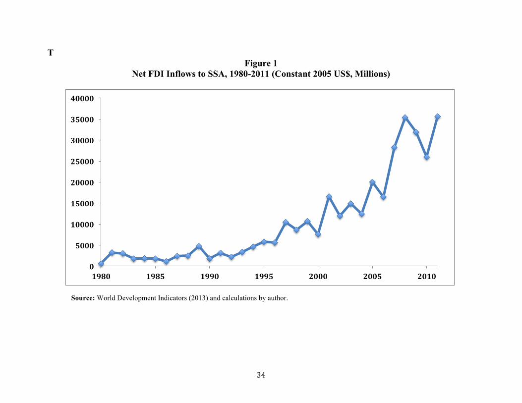
! 34!
T Figure 1
Net FDI Inflows to SSA, 1980-2011 (Constant 2005 US$, Millions)
Source: World Development Indicators (2013) and calculations by author.
0"
5000"
10000"
15000"
20000"
25000"
30000"
35000"
40000"
1980" 1985" 1990" 1995" 2000" 2005" 2010"
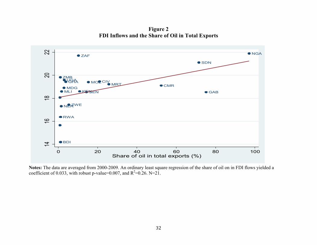
! 32!
Figure 2 FDI Inflows and the Share of Oil in Total Exports
Notes: The data are averaged from 2000-2009. An ordinary least square regression of the share of oil on in FDI flows yielded a coefficient of 0.033, with robust p-value=0.007, and R2=0.26. N=21.
BDI
CMRCIV
GAB
GHA
KENMDG
MLI
MRTMOZ
NER
NGA
RWA
SEN
ZAF
SDN
UGAZMB
ZWE
1416
1820
22
Log o
f net
FDI in
flows
0 20 40 60 80 100Share of oil in total exports (%)
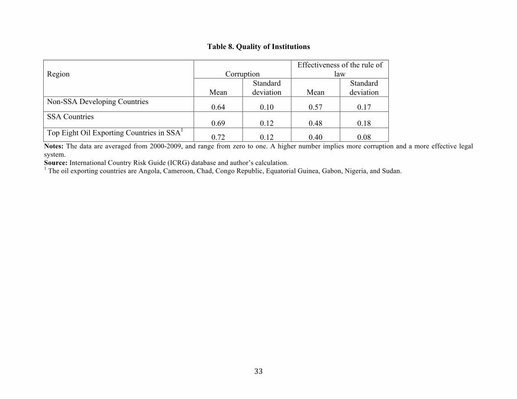
! 33!
Table 8. Quality of Institutions"
Region Corruption
Effectiveness of the rule of law
Mean Standard deviation Mean
Standard deviation
Non-SSA Developing Countries 0.64 0.10 0.57 0.17
SSA Countries 0.69 0.12 0.48 0.18
Top Eight Oil Exporting Countries in SSA1 0.72 0.12 0.40 0.08 Notes: The data are averaged from 2000-2009, and range from zero to one. A higher number implies more corruption and a more effective legal system. Source: International Country Risk Guide (ICRG) database and author’s calculation. 1 The oil exporting countries are Angola, Cameroon, Chad, Congo Republic, Equatorial Guinea, Gabon, Nigeria, and Sudan.
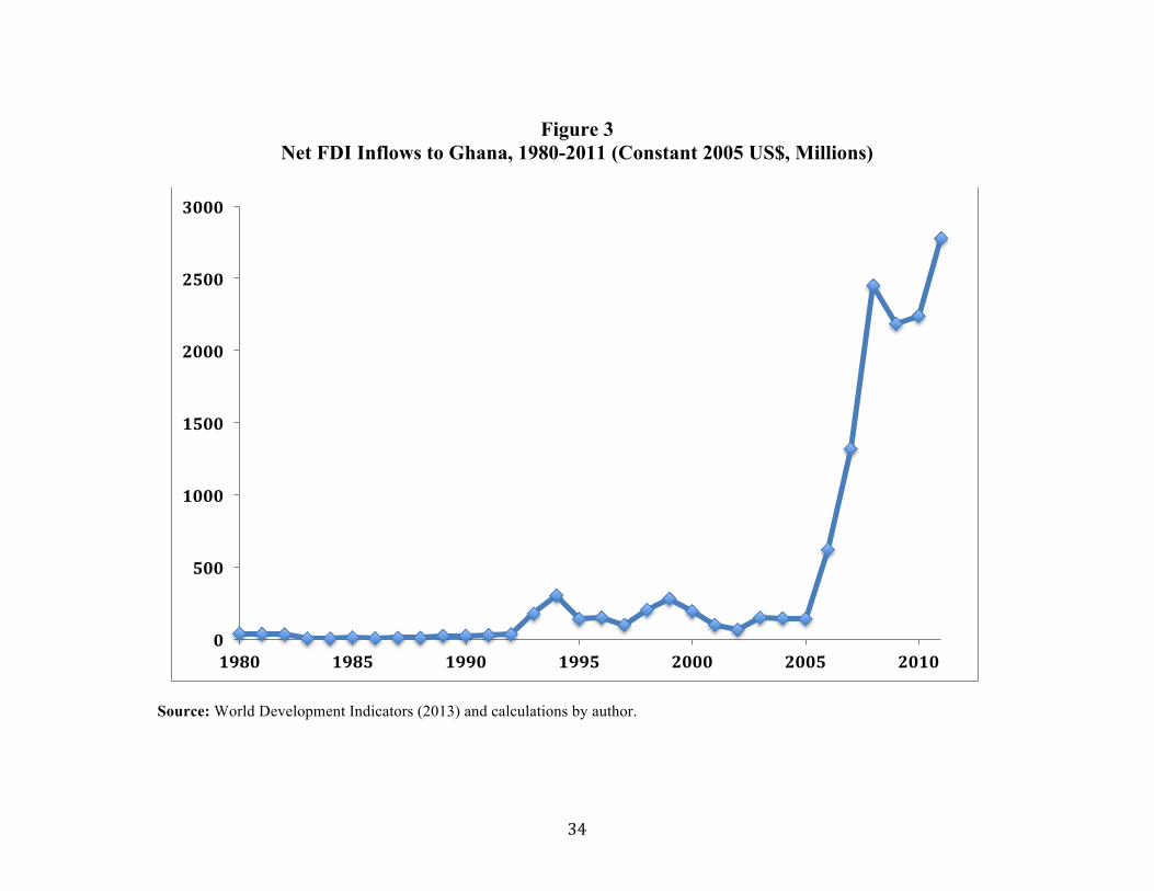
! 34!
Figure 3
Net FDI Inflows to Ghana, 1980-2011 (Constant 2005 US$, Millions)
Source: World Development Indicators (2013) and calculations by author.
! !
0"
500"
1000"
1500"
2000"
2500"
3000"
1980" 1985" 1990" 1995" 2000" 2005" 2010"
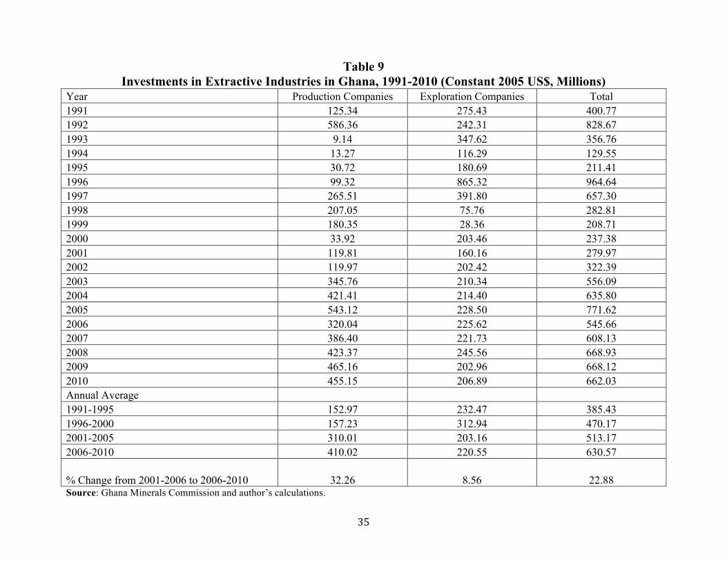
! 35!
Table 9 Investments in Extractive Industries in Ghana, 1991-2010 (Constant 2005 US$, Millions)
Year Production Companies Exploration Companies Total 1991 125.34 275.43 400.77 1992 586.36 242.31 828.67 1993 9.14 347.62 356.76 1994 13.27 116.29 129.55 1995 30.72 180.69 211.41 1996 99.32 865.32 964.64 1997 265.51 391.80 657.30 1998 207.05 75.76 282.81 1999 180.35 28.36 208.71 2000 33.92 203.46 237.38 2001 119.81 160.16 279.97 2002 119.97 202.42 322.39 2003 345.76 210.34 556.09 2004 421.41 214.40 635.80 2005 543.12 228.50 771.62 2006 320.04 225.62 545.66 2007 386.40 221.73 608.13 2008 423.37 245.56 668.93 2009 465.16 202.96 668.12 2010 455.15 206.89 662.03 Annual Average 1991-1995 152.97 232.47 385.43 1996-2000 157.23 312.94 470.17 2001-2005 310.01 203.16 513.17 2006-2010 410.02 220.55 630.57
% Change from 2001-2006 to 2006-2010 32.26 8.56 22.88 Source: Ghana Minerals Commission and author’s calculations.
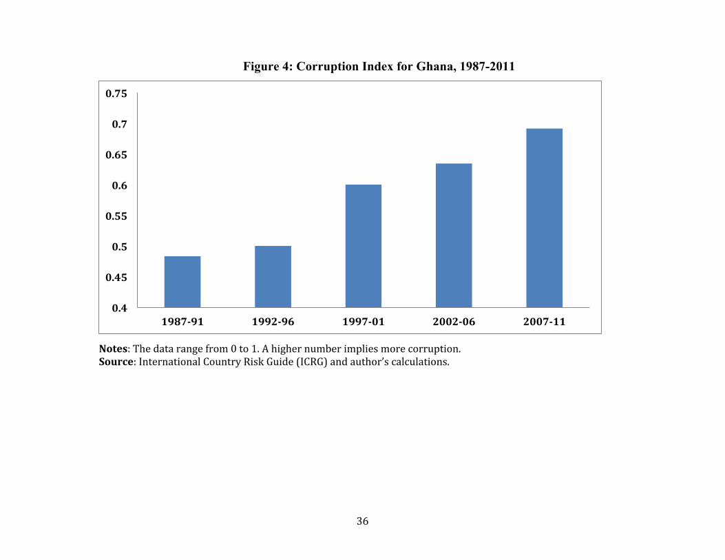
! 36!
Figure 4: Corruption Index for Ghana, 1987-2011
!Notes:!The!data!range!from!0!to!1.!A!higher!number!implies!more!corruption.!!!!!!!!!!!!!!!Source:!International!Country!Risk!Guide!(ICRG)!and!author’s!calculations.!! !
0.4"
0.45"
0.5"
0.55"
0.6"
0.65"
0.7"
0.75"
1987691" 1992696" 1997601" 2002606" 2007611"
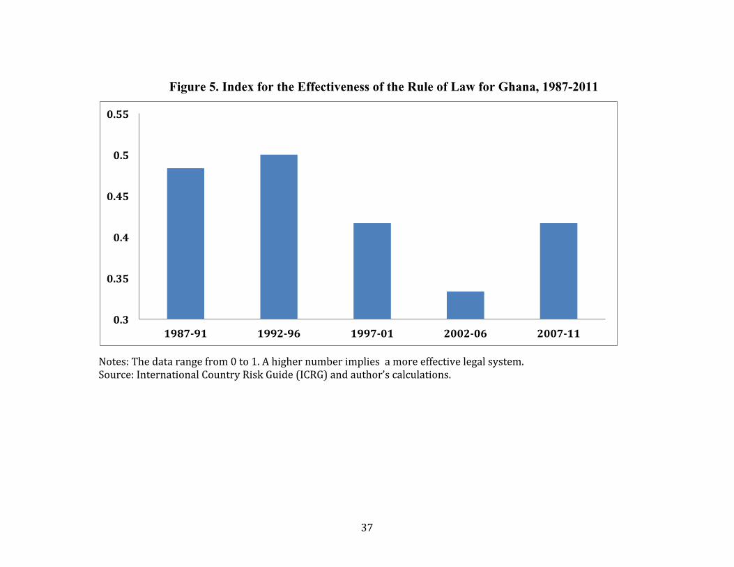
! 37!
!
Figure 5. Index for the Effectiveness of the Rule of Law for Ghana, 1987-2011
!!!!!!!!!!!!!!Notes:!The!data!range!from!0!to!1.!A!higher!number!implies!!a!more!effective!legal!system.!!!!!!!!!!!!!!!!!!!!!!!!!!!!Source:!International!Country!Risk!Guide!(ICRG)!and!author’s!calculations.!! !
0.3"
0.35"
0.4"
0.45"
0.5"
0.55"
1987691" 1992696" 1997601" 2002606" 2007611"

! 38!
!
Table 10
United States Outward FDI Stock in Extractive Industries (Constant 2005 US$, Millions) Region 1995 2000 2005 Growth from 1995-2005 (%) Total World 1,052 853 1,143 9 Developed Countries 642 395 558 -13 Less Developed Countries (LDC) 335 438 498 49 Africa 19 68 112 489 Latin America 92 195 173 88 Middle East 40 25 56 40 South and East Asia 167 131 96 -43 Africa’s share of LDC (%) 5 15 22 Africa’s share of World (%) 1 8 9 Notes: The data for Africa includes SSA and North Africa. Source: UNCTAD 2007 and author’s calculation. !

Table 1A: Countries Included in the Regressions
country FDI/GDP
(%)
Fuel/Exports
(%)
Oil Rents
/GDP (%)
Inst.
Quality
Law &
Order
Government
Stability
FDI Risk Corruption Law &
Order
(Kauffman)
Sub‐Sahara African Countries
Angola 2.780 94.155 29.237 0.421 0.234 0.455 0.497 0.500
Botswana 5.470 0.168 0.000 0.729 0.616 0.849 0.909 0.543 0.621
Burkina Faso 0.966 0.513 0.601 0.629 0.724 0.680 0.372 0.361
Cameroon 1.082 41.248 9.061 0.518 0.418 0.683 0.572 0.401 0.261
Congo, Rep. 3.203 90.358 40.318 0.424 0.378 0.442 0.374 0.500 0.234
Cote d'Ivoire 1.686 17.971 2.358 0.499 0.499 0.590 0.492 0.416 0.259
Ethiopia 2.106 0.598 0.000 0.601 0.797 0.702 0.573 0.333 0.341
Gabon ‐0.022 80.950 41.667 0.487 0.484 0.649 0.594 0.222 0.408
Gambia, The 3.999 0.262 0.624 0.710 0.721 0.598 0.469 0.468
Ghana 2.769 5.614 0.000 0.509 0.395 0.683 0.571 0.385 0.469
Guinea 2.469 0.294 0.544 0.462 0.709 0.507 0.500 0.233
Kenya 0.524 11.105 0.000 0.500 0.460 0.561 0.601 0.376 0.302
Liberia 4.753 0.565 0.318 0.333 0.306 0.465 0.167
Madagascar 2.829 3.073 0.570 0.481 0.603 0.542 0.654 0.406
Malawi 1.343 0.103 0.513 0.473 0.502 0.586 0.492 0.436
Mali 2.501 1.803 0.561 0.500 0.749 0.632 0.365 0.434
Mozambique 5.130 12.820 0.000 0.564 0.488 0.757 0.589 0.421 0.360
Namibia 1.840 0.757 0.000 0.728 0.918 0.859 0.816 0.319 0.533
Niger 0.464 0.850 0.441 0.333 0.680 0.548 0.203 0.334
Nigeria 3.234 95.381 32.773 0.408 0.344 0.572 0.454 0.264 0.247
Senegal 1.193 17.653 0.001 0.546 0.436 0.702 0.587 0.458 0.469
South Africa 1.154 8.929 0.033 0.614 0.427 0.678 0.722 0.628 0.516
Sudan 3.478 48.965 10.010 0.426 0.373 0.642 0.490 0.199 0.205
Tanzania 3.109 0.838 0.000 0.668 0.833 0.827 0.614 0.398 0.425
Togo 1.567 0.515 0.000 0.468 0.430 0.594 0.534 0.313 0.330
Uganda 3.623 1.920 0.609 0.646 0.764 0.670 0.356 0.387
Zambia 5.814 1.415 0.000 0.552 0.616 0.549 0.558 0.486 0.395
Zimbabwe 0.772 2.321 0.000 0.401 0.417 0.552 0.315 0.320 0.225
Other Countries
Albania 4.417 6.522 1.778 0.517 0.452 0.668 0.586 0.360 0.326
Algeria 0.699 96.725 12.084 0.527 0.396 0.690 0.584 0.438 0.322
Argentina 1.892 9.836 3.315 0.526 0.563 0.569 0.462 0.509 0.418
Armenia 6.348 3.506 0.000 0.525 0.506 0.719 0.596 0.277 0.420
Azerbaijan 11.811 84.228 40.085 0.613 0.632 0.806 0.719 0.296 0.319
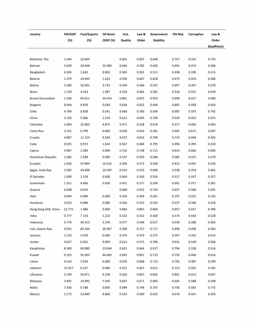
country FDI/GDP
(%)
Fuel/Exports
(%)
Oil Rents
/GDP (%)
Inst.
Quality
Law &
Order
Government
Stability
FDI Risk Corruption Law &
Order
(Kauffman)
Bahamas, The 1.444 22.830 0.601 0.667 0.648 0.757 0.333 0.754
Bahrain 5.638 29.848 23.280 0.646 0.782 0.636 0.691 0.474 0.586
Bangladesh 0.304 1.042 0.003 0.365 0.301 0.511 0.458 0.190 0.315
Belarus 2.379 24.944 1.624 0.596 0.667 0.818 0.475 0.424 0.286
Bolivia 3.300 32.091 3.714 0.439 0.366 0.547 0.497 0.347 0.379
Brazil 1.729 4.333 1.487 0.528 0.481 0.581 0.518 0.531 0.439
Brunei Darussalam 1.596 94.611 34.410 0.801 0.875 0.953 0.958 0.417 0.580
Bulgaria 8.944 9.659 0.030 0.634 0.625 0.646 0.805 0.458 0.454
Chile 4.784 0.838 0.341 0.660 0.760 0.596 0.687 0.597 0.742
China 3.156 5.066 2.554 0.612 0.695 0.740 0.559 0.453 0.415
Colombia 2.464 32.963 4.875 0.471 0.238 0.614 0.577 0.456 0.364
Costa Rica 3.251 0.799 0.000 0.628 0.654 0.581 0.605 0.673 0.607
Croatia 4.887 11.154 0.550 0.672 0.816 0.709 0.719 0.444 0.492
Cuba 0.025 0.973 1.624 0.567 0.684 0.795 0.396 0.395 0.320
Cyprus 4.987 2.383 0.000 0.732 0.738 0.711 0.814 0.666 0.696
Dominican Republic 2.582 1.589 0.000 0.537 0.503 0.586 0.585 0.472 0.379
Ecuador 1.656 47.894 16.316 0.509 0.572 0.560 0.415 0.491 0.336
Egypt, Arab Rep. 2.585 43.698 10.595 0.533 0.555 0.696 0.528 0.354 0.491
El Salvador 1.040 2.139 0.000 0.460 0.330 0.556 0.517 0.437 0.357
Guatemala 1.351 4.066 0.630 0.451 0.277 0.549 0.601 0.377 0.281
Guyana 6.648 0.010 0.608 0.552 0.743 0.637 0.500 0.391
Haiti 0.094 0.000 0.000 0.334 0.394 0.431 0.197 0.315 0.165
Honduras 3.033 0.984 0.000 0.436 0.322 0.545 0.537 0.340 0.318
Hong Kong SAR, China 22.775 1.986 0.000 0.806 0.807 0.804 0.957 0.657 0.784
India 0.777 7.133 1.222 0.532 0.552 0.569 0.574 0.434 0.528
Indonesia 0.776 36.413 5.376 0.477 0.446 0.617 0.558 0.288 0.365
Iran, Islamic Rep. 0.951 82.104 29.467 0.598 0.727 0.717 0.490 0.458 0.364
Jamaica 3.233 5.559 0.000 0.474 0.370 0.575 0.597 0.352 0.415
Jordan 4.657 0.201 0.004 0.613 0.575 0.706 0.631 0.540 0.566
Kazakhstan 8.369 60.080 23.044 0.651 0.664 0.917 0.704 0.318 0.314
Kuwait 0.193 92.093 44.683 0.695 0.851 0.733 0.750 0.446 0.616
Latvia 4.524 3.594 0.000 0.676 0.808 0.713 0.795 0.387 0.599
Lebanon 12.427 0.327 0.000 0.551 0.667 0.612 0.723 0.201 0.392
Lithuania 3.799 20.871 0.258 0.636 0.667 0.665 0.801 0.413 0.607
Malaysia 3.942 14.995 7.345 0.647 0.671 0.683 0.645 0.588 0.598
Malta 7.436 0.788 0.000 0.699 0.748 0.707 0.758 0.585 0.772
Mexico 2.175 23.840 6.866 0.553 0.469 0.625 0.676 0.441 0.392

country FDI/GDP
(%)
Fuel/Exports
(%)
Oil Rents
/GDP (%)
Avg. Inst.
Quality
Law &
Order
Government
Stability
FDI Risk Corruption Law &
Order
(Kauffman)
Moldova 5.710 0.298 0.051 0.587 0.817 0.740 0.504 0.287 0.417
Mongolia 5.142 2.611 0.355 0.611 0.667 0.712 0.586 0.479 0.482
Morocco 1.211 2.583 0.008 0.627 0.704 0.728 0.612 0.463 0.502
Nicaragua 3.899 0.853 0.000 0.538 0.513 0.536 0.473 0.628 0.354
Oman 1.605 83.654 34.103 0.679 0.757 0.763 0.729 0.468 0.620
Pakistan 1.059 2.276 0.642 0.448 0.431 0.582 0.465 0.316 0.339
Panama 4.105 3.358 0.000 0.488 0.438 0.575 0.605 0.333 0.466
Papua New Guinea 3.197 12.398 14.444 0.513 0.519 0.578 0.526 0.428 0.316
Paraguay 1.384 0.113 0.000 0.478 0.453 0.564 0.661 0.236 0.300
Peru 2.487 10.569 2.654 0.472 0.383 0.498 0.540 0.468 0.368
Philippines 1.293 1.686 0.079 0.450 0.376 0.517 0.570 0.335 0.435
Qatar 4.380 85.972 23.152 0.755 0.868 0.940 0.830 0.382 0.636
Romania 3.327 7.759 1.762 0.604 0.702 0.619 0.602 0.494 0.480
Russian Federation 1.936 53.017 12.974 0.583 0.611 0.802 0.603 0.314 0.317
Saudi Arabia 1.957 90.984 38.488 0.641 0.764 0.711 0.711 0.377 0.530
Singapore 12.170 14.253 0.000 0.812 0.877 0.800 0.804 0.767 0.798
Sri Lanka 1.084 1.840 0.000 0.499 0.364 0.550 0.571 0.511 0.524
Suriname ‐8.513 2.210 5.676 0.458 0.387 0.571 0.426 0.447 0.445
Syrian Arab Republic 0.873 61.078 19.075 0.551 0.618 0.727 0.440 0.420 0.412
Thailand 2.512 2.181 0.442 0.566 0.617 0.635 0.605 0.406 0.545
Trinidad and Tobago 5.818 63.860 14.298 0.578 0.604 0.616 0.669 0.424 0.543
Tunisia 2.571 17.425 4.718 0.598 0.646 0.701 0.595 0.452 0.496
Turkey 0.886 2.777 0.253 0.568 0.615 0.639 0.569 0.450 0.496
Ukraine 3.745 6.857 0.950 0.532 0.667 0.630 0.499 0.332 0.318
United Arab Emirates 3.621 71.896 19.115 0.697 0.667 0.880 0.905 0.336 0.609
Uruguay 1.822 1.244 0.000 0.567 0.472 0.624 0.667 0.505 0.606
Venezuela, RB 1.495 84.867 25.181 0.485 0.536 0.625 0.388 0.393 0.264
Vietnam 5.951 20.346 8.118 0.640 0.713 0.856 0.614 0.375 0.415
Yemen, Rep. 1.691 81.624 28.731 0.539 0.404 0.741 0.595 0.415 0.249
The data in the table are the averages for each country for the sample period of 1984 to 2011. The institutional quality variables (Law and
order, Government Stability, Corruption, FDI Risk, Law and Order (Kauffman) and Average Institutional Quality) have been normalized to fall
between zero and one.
Designed by soapbox.co.uk
The International Growth Centre (IGC) aims to promote sustainable growth in developing countries by providing demand-led policy advice based on frontier research.
Find out more about our work on our website www.theigc.org
For media or communications enquiries, please contact [email protected]
Subscribe to our newsletter and topic updates www.theigc.org/newsletter
Follow us on Twitter @the_igc
Contact us International Growth Centre, London School of Economic and Political Science, Houghton Street, London WC2A 2AE