direct numerical simulation of compressible °ow over a ... · direct numerical simulation of...
TRANSCRIPT

Direct numerical simulation of compressible
flow over a backward-facing step
K. Sengupta, K. K. Q. Zhang and F. Mashayek
Department of Mechanical and Industrial Engineering
University of Illinois at Chicago
G. B. Jacobs
Department of Aerospace Engineering and Engineering Mechanics
San Diego State University
March 25, 2009
Abstract
In this paper, we perform a direct numerical simulation study to investigative the effect of
compressibility on the flow over a backward-facing step. A spectral multidomain method is used
for simulating the compressible flow at Reynolds number of 3000 over an open backward-facing
step. The role of compressibility in the sub-sonic regime is studied by simulating the flow at
different free-stream Mach numbers.
We analyze the effect of compressibility on the averaged flow and the Reynolds stresses.
Results indicate that the effect of compressibility on the separated and reattached shear layer
in the backward-facing step is different from that on spatial and temporal mixing layers studied
1
previously. While the canonical free shear flows exhibit a reduction in growth rate with increase
in Mach number, the shear layer in the present study shows an opposite trend. We compute
the budget of turbulent kinetic energy to determine the plausible causes of such behavior. We
conclude that a greater turbulence production for higher Mach numbers is primarily responsible
for the larger growth rate of the shear layer.
1 Introduction
Separating and reattaching turbulent flows have immense technological implications. They
occur in many practical devices like diffusers, combustors and around airfoils and bluff bodies
to name a few. Flow over a backward-facing step (BFS) is a configuration that is often studied
to understand the physics of separated flows. Moreover, combustors and afterburners in ramjet
engines are modeled after such geometries. The flow dynamics in BFS can be decomposed as
follows: The boundary layer upstream of the step separates at the step corner, becoming a free
shear layer. The free shear layer expands over the step and creates a recirculation region, before
reattaching to the bottom wall. The flow subsequently recovers to an equilibrium boundary
layer profile.
Since the pioneering experimental study by Eaton and Johnston1 there has been consider-
able amount of research into backward-facing step flows. Armaly et al.2 presented experimental
studies on the effect of Reynolds number on the reattachment length for a given expansion ratio.
The flow appeared to be three-dimensional for Reynolds number (based on the step height and
the inlet free stream velocity) above 400. The reattachment length was found to increase with
Reynolds number upto 1200, then decreased in the transitional range 1200 < Re < 6600 and
finally remained relatively constant in the fully turbulent range (Re > 6600). The effects of
expansion ratio on the reattachment length were studied by Durst and Tropea3. The reattach-
2

ment length also depends on the state of the flow at separation and the ratio of the boundary
layer thickness to step height. Adams et al.4 investigated the effect of upstream boundary layer
profile on the reattachment length. The effect of inlet turbulence intensity on the reattachment
process was studied by Isomoto and Honami5.
Numerous computational studies have also been conducted for BFS flow in the past two
decades. Most of the early numerical simulations have been confined to two-dimensional flows.
Kim and Moin6 used a fractional step method to compute incompressible two-dimensional flow.
The discrepencies with the experimental data of Armaly et al.2 were attributed to the onset
of three-dimensionality above Reynolds number 600. Kaikatis et al.7 identified bifurcation of
two-dimensional laminar flow to three-dimensional flow at Rec=700, as the primary source of
mismatch between simulation and experimental data. In a later work8 Kaikatis found that
the unsteadiness was created by convective instabilities. Le et al.9 conducted the first direct
numerical simulation for a three-dimensional backward-facing step configuration for a Reynolds
number (based on step height and free stream velocity) of 5100 and expansion ratio (ratio of
the height of the post expansion section to that of the inlet channel) of 1.2. Their results
were compared with the experiment of Jovic and Driver10. In addition to typical engineering
quantities, such as averaged skin friction and pressure coefficients, Le et al.9 reported on the
unsteady characteristics of the flow. The mean streamwise velocity and Reynolds stresses in
the recirculation, reattachment and recovery regions compared well with the experimental data.
They also computed the budgets of turbulent kinetic energy and Reynolds stresses. Kaltenbach
and Janke11 investigated the effect of ‘sweep’ on transitional separation bubble behind the step.
Sweeping essentially amounts to skewing the inlet velocity profile in the spanwise direction.
In their baseline unswept case at Re=3000, the boundary layer at the step was laminar and
underwent transition before reattaching. A similar configuration was later simulated by Wengle
et al.12 More recently, Barkley et al.13 carried out three-dimensional linear stability analysis for
3
an expansion ratio of 2. They showed that the primary bifurcation of the steady, two-dimensional
flow is a steady, three-dimensional instability.
The computational studies mentioned above have dealt with incompressible flows. Renewed
interest in high speed propulsion has invigorated fundamental research on compressible tur-
bulent flows (see Lele14 for a review). Compressibility effects have been studied in detail for
free shear flows. Stabilizing effect of compressibility has been one of the most distinguish-
ing features of compressible shear flow from its incompressible counterpart. The convective
Mach number Mc, introduced by Bogdanoff15 is the most widely used parameter for determin-
ing compressibility effects. For streams with equal specific heats the convective Mach number,
Mc = (U1 − U2)/(c1 + c2), where U1, U2 are free stream velocities and c1, c2 are the free stream
sound speeds. A number of studies (see e.g. Papamoschu and Roshko16, Hall et al.17, Clemens
and Mungal18) have shown large reduction in growth rate with increasing Mc. Several different
explanations for inhibited growth rate of shear layer have been offered. Zeman19 and Sarkar20
proposed that dilatational dissipation and pressure-dilatation, which acts as sink of turbulent
kinetic energy, could at sufficiently high Mach numbers lead to reduction in turbulence levels
and thereby inhibit shear layer growth. However, the above explanation was later replaced by
alternate theories by Sarkar21 and Vreman et al.22, which indicated that reduced turbulent pro-
duction, and not the dilatation terms, was responsible for decreased turbulent kinetic energy.
A direct relationship between momentum thickness growth rate and the integrated turbulent
production was established for the mixing layer by Vreman et al.22 They further showed that the
reduction in turbulent production is due to reduced pressure fluctuation via the pressure-strain
term. For uniform shear flow, Sarkar23 found that the pressure gradient term in the momentum
equation and the pressure-strain term in the Reynolds stress equation lead to reduced turbulence
levels. Freund et al.24 also confirmed the reduction of the pressure strain term in the annular
mixing layer. In their DNS study, Pantano and Sarkar25, showed that the gradient Mach num-
4

ber, which is the ratio of the acoustic time scale to the flow distortion time scale, is the key
parameter which determines the reduction in pressure-strain term in compressible shear flows.
There has been dearth of LES/DNS studies of compressible separating and reattaching flows.
Avancha and Pletcher26 carried out large-eddy simulation of flow over a backward-facing step
with wall heat flux at single low Mach number of 0.006. The focus of their study was to analyze
the heat transfer characteristics in the flow. Their major conclusions were an occurrence of
peak heat transfer rate slightly upstream of the reattachment, and invalidation of the Reynolds
analogy within the recirculation zone. In a recent study, Dandois et al.27 carried out direct
numerical and large-eddy simulation of flow over a rounded ramp at a single free stream Mach
number 0.3. The motivation of the study was to control the separation using synthetic jets at
different frequencies. Numerical simulation of a compressible mixing layer past an axisymmetric
trailing edge was performed by Simon et al.28. The work focussed on evolution of the turbulence
field through extra strain rates (owing to streamline curvature) and on the unsteady features of
the annular shear layer at a single Mach number of 2.46. A hybrid RANS/LES methodology
called zonal detached eddy simulation (ZDES) was used for computing the flow at a Reynolds
number (based on the diameter of the trailing edge) of 2.9 million. A three-dimensional stability
study of compressible flow over open cavities was conducted by Bres and Colonius29. They
performed both linear stability analysis and direct numerical simulation. The authors concluded
that instability mode properties were by and large unaffected by Mach number over a subsonic
range upto 0.6.
As is seen from a survey of the available literature, interest in DNS and LES of compressible
separated shear flows in practical applications has grown only recently. Moreover, there has
been only few studies of the backward-facing step configuration, none of which attempted to
evaluate the role of compressibility. In this context, the present direct numerical computation of
compressible flow over a backward-facing step is an attempt to improve physical understanding
5

of this benchmark flow by looking at different flow statistics and energy budget. The work seeks
to address open questions such as: How does the mean flow and turbulent stresses change with
free stream Mach number? How does the free-stream Mach number affect the growth of the
shear layer? What are the contributions of various quantities in the budget of turbulent kinetic
energy? Paucity of computational resources restricts our investigation to the low Reynolds
number regime. The paper is organized as follows: First we describe the governing equations
in section 2. In section 3, a brief account of our numerical methodology is provided. The
backward-facing step model is described in section 4. In section 5, we validate our simulation
by comparing the mean flow and second order statistics with experiment. The flow topology
is described in section 6. The budget of turbulent kinetic energy is presented and analyzed in
detail in section 7. Finally we summarize the important findings in section 8.
2 Governing Equations
The governing equations for the compressible and viscous fluid flow are the conservation state-
ments for mass, momentum and energy. They are presented in non-dimensional, conservative
form with Cartesian tensor notation,
∂ρ
∂t+
∂(ρuj)
∂xj
= 0, (1)
∂(ρui)
∂t+
∂(ρuiuj + pδij)
∂xj
=∂σij
∂xj
, (2)
∂(ρe)
∂t+
∂[(ρe + p)uj]
∂xj
= − ∂qj
∂xj
+∂(σijui)
∂xj
. (3)
The total energy, viscous stress tensor and heat flux vector are, respectively, given as,
ρe =p
γ − 1+
1
2ρukuk, (4)
6
σij =1
Re
(∂ui
∂xj
+∂uj
∂xi
− 2
3
∂uk
∂xk
δij
), (5)
qj = − 1
(γ − 1)RePrM2f
∂T
∂xj
. (6)
The Reynolds number Re is based on the reference density ρ∗f , velocity U∗f , length L∗f , and
molecular viscosity µ∗f and is given by Re = ρ∗fU∗f L∗f/µ
∗f . Pr = µ∗fCp/k
∗ is the Prandtl number.
The superscript ∗ denotes dimensional quantities. The above equation set is closed by the
equation of state,
p =ρT
γM2f
, (7)
where Mf is defined as Mf = U∗f /c∗f , with c∗f =
√γRT ∗
f denoting the reference speed of sound.
Here, Tf is the reference temperature. Therefore, by definition Mf is the reference Mach number,
which is taken as 1 implying that our reference velocity is the same as the reference speed
of sound. The flow Mach number, which does not appear explicitly in the non-dimensional
equations is defined as, M = U∗f /c∗, where c∗ now is given by, c∗ =
√γRT ∗. With Mf set to
unity, M essentially becomes the reciprocal of the non-dimensional sound velocity. Moreover,
from the above definitions, M (which is a local quantity in the flow) is related to the local non-
dimensional temperature T ∗/T ∗f . In the simulations presented in this paper, the “free-stream”
M , based on the non-dimensional temperature at the wall, is varied to obtain results at different
Mach numbers. The conservation equations can be cast in the matrix form
∂Q
∂t+
∂F ai
∂xi
− ∂F vi
∂xi
= 0, (8)
where
Q =
ρ
ρu1
ρu2
ρu3
ρe
, (9)
7

F ai =
ρui
ρu1ui + pδi1
ρu2ui + pδi2
ρu3ui + pδi3
(ρe + p)ui
, (10)
F vi =
0
σi1
σi2
σi3
−qi + ukσik
. (11)
Here, Q is the vector of the conserved variables, while F ai and F v
i are the advective and viscous
flux vectors respectively, in the xi direction.
3 Numerical Method
In this work, a staggared grid Chebyshev multidomain method is used for solving the governing
transport equations. Here, we provide a brief description of the method. For a more complete
description, the reader is referred to our previous works30–32. The approximation begins with the
subdivision of the computational domain into non-overlapping hexahedral subdomains/elements.
Each element is then mapped onto a unit hexahedron by an isoparametric transformation using
a linear blending formula. Under the mappings, Eq. (8) becomes
∂Q
∂t+
∂F ai
∂Xi
− ∂F vi
∂Xi
= 0, (12)
where
Q = JQ,
F ai =
∂Xi
∂xj
F aj ,
F vi =
∂Xi
∂xj
F vj . (13)
8

In the above equations, Q and Q represent the solution vectors (Eq. (9)) on the physical and
the mapped grid, respectively. J is the Jacobian of the transformation from the physical space
to the mapped space. The fluxes (Eqs. (10) and (11)) on the two grids are given by F and F ,
while the term ∂Xi
∂xjis the metric of the transformation, xj and Xi being the coordinates of the
physical space and the mapped space, respectively.
Within each sub-domain the solution values, Q, and the fluxes, F i, in Eq. (12) are ap-
proximated on separate grids. The solutions are computed on the Chebyshev-Gauss grid while
the fluxes are computed on the Chebyshev-Gauss-Lobatto grid. In one space dimension, the
Chebyshev-Gauss and Chebyshev-Gauss-Lobatto quadrature points are defined by,
Xj+1/2 =1
2
{1− cos
[(2j + 1)π
2N
]}, j = 0, ....N − 1, (14)
and
Xj =1
2
{1− cos
[πj
N
]}, j = 0, ....N, (15)
respectively, on the unit interval [0, 1]. In three-dimension, the corresponding grids are given by
the tensor product of the above one-dimensional grids. Thus the solution is approximated as,
Q(X, Y, Z) =N−1∑
i=0
N−1∑
j=0
N−1∑
k=0
Qi+1/2,j+1/2,k+1/2hi+1/2(X)hj+1/2(Y )hk+1/2(Z), (16)
where hj+1/2 ∈ PN−1 is the Lagrange interpolating polynomial defined on the Gauss grid.
The computation of the advective (inviscid) and viscous fluxes follow different procedures.
The inviscid fluxes are computed by reconstructing the solution at the Gauss-Lobatto points
using the interpolant (Eq. (16)). This, however, leads to two different flux values at the sub-
domain interface points, one from each of the two contributing sub-domains. In-order to enforce
continuity of the fluxes, Roe’s approximate Riemann solver33 is used to compute a single flux
from the two values. For a detailed description of the role of the Riemann solver, we refer to
Kopriva and Kolias34.
9

The computation of the viscous flux uses a two-step procedure. Since the reconstruction of
the solution from the Gauss points onto the Lobatto points gives a discontinuous solution at the
element faces, it is necessary to construct first a continuous piecewise polynomial approximation
before differentiating. To construct the continuous approximation, the average of the solutions
on either side of the interface is used as the interface value. The continuous solution is then dif-
ferentiated to obtain the derivative quantities needed for the viscous fluxes. Since differentiation
reduces the polynomial order by one, it is natural to evaluate the differentiated quantities on
the Gauss grid. Once the derivative quantities are evaluated at the Gauss points, a polynomial
interpolant of the form (Eq. (16)) is defined, so that the gradients can be evaluated at the Lo-
batto points. From the cell face values, the viscous fluxes are computed and combined with the
inviscid fluxes to obtain the total flux. Finally, a semi-discrete equation for the solution values
is obtained by computing the gradient of the total fluxes at the Gauss points. The equation is
advanced in time using a 4th-order low storage Runge-Kutta scheme.
Note that evaluating the gradients at the cell centers has two desired effects. First, it makes
the evaluation of the divergence consistent with that used in the continuity equation. Second,
the evaluation of the viscous fluxes will not require the use of sub-domain corner points.
4 Computational Model
To the best of the authors’ knowledge there has not been any experiment for compressible flow
over backward-facing step in the Reynolds number regime that is feasible for DNS. In this work
we simulate the backward-facing step geometry investigated by Wengle et al.12 (hereafter referred
to as WHBJ). The WHBJ experiment was conducted for incompressible flow at a single Reynolds
number of 3000. Figure 1 shows the computational domain used in this study. The streamwise
length (L) is 22.92h including an inlet section Li = 5h, where h is the step-height taken as 1. The
10

total height in the z-direction is 11.76. The spanwise extent is taken to be 6h. The co-ordinate
system is placed at the lower left corner of the domain as shown in the figure. The multi-
domain spectral method allows control of resolution at two levels: the number of sub-domains
(h-resolution) and polynomial order within each sub-domain (p-resolution). The number of
sub-domains employed for the inlet section are hx = 8, hy = 12, hz = 6. The distribution of sub-
domains in the x-direction and z-direction conforms to a power-law, while uniform element sizes
are considered in the y-direction. For x > 5, a similar power law distribution with 32 elements is
used in the x-direction. The region behind the step (z < 1) is discretized with 6 sub-domains in
the z-direction having a cosine distribution. The region above the step (z > 1) has 6 sub-domains
with a power law distribution. As with the inlet section, uniform spacing of 12 elements is used
in the y-direction. The above distribution gives finer grid at the step corner, in the shear layer
and in the boundary layer.
4.1 Initial and boundary conditions
At the inlet (x = 0), following Ref.12, a laminar boundary layer profile with δ0.99/h = 0.21 is
imposed. The density is set to ρ∞ = 1.0, while the temperature is set to 1/M2. Pressure is
obtained from the density and temperature using the equation of state (Eq. (7)). At the top
boundary z = 11.76, the primitive flow variables are set to the same freestream values as in the
inflow. The outflow boundary conditions for the multi-domain Chebyshev spectral method have
been studied by Jacobs et al.35. The outflow boundary condition employed here follows the
Boundary SPECified (BSPEC) condition described in Ref.35 The exterior state value for the
streamwise velocity, u, is the average velocity profile extracted from WHBJ. The pressure is set
to its free stream value p∞, with the expectation that at a far distance from the step the flow
will return to its free stream state. Conservative isothermal wall boundary condition of Jacobs
et al.31 is used at the wall with the wall temperature set to 1/M2. The Reynolds number based
11

on the step height and the velocity outside the boundary layer (U∞) at the step is 3000, same
as in WHBJ.
The flow at z > 1 is initialized with the uniform inlet condition while for z < 1 all the
variables are set to zero. This ensures that mass is conserved initially and since the method is
conservative, mass conservation is ensured throughout the computation.
5 Validation and Convergence Study
The purpose of this section is to validate our numerical methodology by comparing with the
measurements of WHBJ. Several cases investigated are listed in table 1. All simulations are
conducted in three stages: (1) establish a stationary turbulence, (2) calculate averages, and (3)
calculate fluctuations and related statistics. The simulation is run for approximately 10 flow-
through times to reach the statistically stationary state. The mean statistics are then computed
for over 5 flow-through times and finally another 10 flow-through times are used to compute the
higher order statistics. The dimensional flow-through time is given by L/U∞, the time required
by a fluid particle to traverse the length of the computational domain. Compressibility effects
are expected to be small for Ma2 (the lowest Mach number case) and therefore, Ma2 will be
treated as the base case for comparison with the incompressible experiment12.
Reattachment length
The size of the mean recirculation vortex is used as an important global measure for deter-
mining the accuracy of backward-facing step computations9;36. The size of the recirculation
region is characterized by the reattachment length, Lr. Reattachment length is the distance
from the step wall to the point of zero wall shear stress (τw = 0 or dU/dz = 0). Its value
depends on various parameters, such as (a) Reynolds number based on the step height, Reh,
(b) state of the flow at the separation, (c) the ratio of boundary layer thickness to step height
12

at the edge of the step, (d) turbulence intensity in the free stream and (e) expansion ratio.
The mean reattachment lengths reported in WHBJ are Lr = 6.4 and Lr = 6.5 for experiment
and computations, respectively. Table 1 shows the mean reattachment length for all the cases
along with the magnitude of deviation from the above experimental value. Clearly, free stream
Mach number affects the reattachment location, which is closer to the step for higher Mach
numbers. Ma2 provides the closest agreement with the experiment. Further reduction in Mach
number (≈ 0.1) leads to severe limitation on the time step resulting in inordinately large total
computational time. Therefore, we restricted the lowest Mach number in our study to 0.2. The
physical origin of the variation in reattachment length with Mach number will be discussed in
Section 7.
Averaged velocity
We undertake a systematic comparison of our simulation results with the averaged velocity
data from the experiment in WHBJ. One of the distinguishing aspects of our spectral multido-
main method is the feature of controlling the spatial resolution at two different levels. The
resolution can be altered either by changing the number of sub-domains (h-refinement) or by
changing the order of the polynomial within each sub-domain (p-refinement). The theory of
h/p convergence37 indicates that p-refinement has exponential convergence while h-refinement
leads to only an algebraic convergence rate. Therefore, we conduct a p-convergence study for
our backward-facing step simulations at Ma=0.4 with three different polynomial orders, p=6,
8, 10, the corresponding cases denoted by Ma4, Ma4-p8 and Ma4-p10 in table 1. Figure 2 plots
the Favre averaged streamwise and wall normal velocities for the different polynomial orders,
in the recirculation (x/H = 3, 4), reattachment (x/H = 5) and recovery region (x/H=6). The
figure indicates that the differences resulting from an increase in polynomial order are small.
Therefore, the mean flow is well resolved with the lowest polynomial order (p=6). At stations
x/H = 4 and x/H = 5 we observe significant differences with experiment values. The differ-
13

ences are amplified for the wall normal velocity, due to their smaller range compared to the
streamwise velocity. The fair agreement in the mean velocities for Ma=0.4 is consistent with
the underprediction of the mean reattachment length (see table 1). The obvious physical differ-
ence between the experiment and our simulations at Ma=0.4 is compressibility. This argument
is supported in figure 3, where the Favre averaged velocities for different Mach numbers are
plotted. Ma2 profiles are in good agreement with the experiment, implying that increasing the
free-stream Mach number can significantly alter the averaged flow field for the backward-facing
step geometry.
Reynolds stresses
In turbulent shear flows, the Reynolds stresses (second-order turbulent statistics) are harder
to predict than the averaged quantities (first-order statistics). As before, we establish p-
convergence for the second-order statistics by analyzing normal and shear stresses for Ma4 and
Ma4-p8. Figure 4 shows the streamwise normal stress and shear stress at different streamwise
locations, downstream of the step. Good agreement between the two cases confirms that p=6
provides adequate resolution even for the second-order statistics. The small cusps in the pro-
files in figure 4 are an artifact of the discontinuity of the solution at the sub-domain interfaces,
which is inherent in our multi-domain spectral method. Since Reynolds stresses are given by the
covariances of the solution variables (velocities), any discontinuity at the interface points will
naturally have more impact on them than on the averaged quantities (figures 2 and 3), where no
cusps appear. It must be noted that lack of smoothness does not imply lack of accuracy. The
discontinuity in the solution across the sub-domains will reduce with increase in the polynomial
order of approximation. This is confirmed in figure 4, where using p=8 results in smoother
profiles than p=6.
WHBJ provides measurements of streamwise normal stress {uu} and shear stress {uw}, which
are compared with our simulation results in figure 5. The separating boundary layer is laminar,
14

confirmed by the low intensity levels (0.3%) just upstream of the step. Figure 5 reveals a
large difference in both normal and shear stresses between Ma2 and the higher Mach number
cases in the recirculation region (x/H = 4). This implies a faster transition to turbulence for the
separated shear layer at higher Mach numbers, resulting in a more turbulent recirculation region.
Differences between the experiment and the base case (Ma2) is consistent with the findings
in WHBJ, where similar differences between experiment and computation were observed. At
x/H = 6, Ma3 and Ma4 seem to agree better with the experiment, but this to the authors
opinion is more fortuitous than physical and can be explained from the streamwise location of
the profiles for each case relative to the reattachment point. The station x/H = 6 is near the
reattachment point for Ma2 (Lr = 6.0), but lies in the early recovery region of the flow for
Ma3 (Lr = 5.45) and Ma4 (Lr = 5.42), while in the experiment the location is still half a step
height away from the reattachment point. As the flow evolves, the turbulent stresses increase
upto the reattachment point and then start to decay downstream of it. Therefore, the Reynolds
stresses for Ma3 and Ma4, representative of the early recovery region are incidentally closer to
the experiment, corresponding to the backflow region, than are the stresses for Ma2. Further
downstream, x/H = 8, stresses for Ma2 are again closer to the experiment than Ma3 and Ma4,
consistent with the overall trend.
6 Flow Topology
Topology of the three-dimensional flow over a backward-facing step is very complex. The flow
structures have been investigated in the studies by Neto et al.36 Figure 6 shows the pressure
iso-contours for the case Ma4. Pressure iso-contours provide a good indicator of various vortical
structures since at the center of a viscous vortex pressure has a minimum and increases radially
outward38. The iso-contour at any radial distance from the pressure minima visualizes the
15

vortex through a closed contour. The figure shows that as the shear layer goes into transition,
two-dimensional Kelvin-Helmhotz billows are created at about 3 step heights downstream of
the step. These spanwise rollers, though nominally two-dimensional, still exhibit waviness in
the spanwise direction. As the shear layer grows, the vortices start interacting (helical pairing)
and transform into staggered arch-like vortices which impact the lower wall at the reattachment
region. The accompanied bursting of these structures upon impact, creates three-dimensional
longitudinal vortices.
The underlying vorticity field in the flow can be visualized using the concept of helicity.
Formally, helicity for a fluid confined to a domain D, is the integrated scalar product of the
three-dimensional velocity and vorticity field39,
H =∫
D
~U · ~ωdV (17)
where ~U and ~ω are the velocity and vorticity, respectively. Physically, helicity can be interpreted
as the extent of “cock screw” like motion present in the flow. Regions of high helicity indicate
that the axis of rotation of the local fluid elements is aligned with the fluid velocity. Therefore,
helical structures are located by identifying vortices that have non zero velocity along their
axes. Figure 7 depicts helical structures represented by vortex cores, colored by the streamwise
velocity. The vortex cores are located by finding cells in which vorticity is aligned with velocity.
Cells in which two or more faces of the cell have this criterion are determined to have been
pierced by the core center-line. Clustering of vortex cores in the shear layer indicates a strong
“cock screw” type motion of the fluid. Qualitative changes in the flow resulting from vortex
breakdown are presumably closely related to large changes in helicity39, which may therefore be
used to characterize such events. Decrease in vortex cores (figure 7) beyond the reattachment
region implies breakdown of the coherent structures as the shear layer impinges on the bottom
wall.
16

7 Analysis of Compressibility Effects
Analysis of the averaged flow field and Reynolds stresses shows that the change in the free-
stream Mach number affects the flow. A shorter reattachment length with increase in Mach
number indicates that the separated shear layer over a backward-facing step is less stable with
increase in compressibility. This behavior is different from free shear layers, where compress-
ibility suppresses the growth rate thereby promoting stability. Before analyzing the probable
physical mechanism responsible for such anomalous behavior, we would like to verify that our
numerical methodology is able to capture the effect of compressibility on a classical free-shear
layer. This verification serves two purposes: first it provides an additional validation of our
methodology and second it would indicate that the opposite trend observed for the shear layer
in the backward-facing step has a physical origin.
Therefore, in the following sub-section we simulate a compressible free shear layer at different
Mach numbers. The rest of the section is devoted to the detailed analysis of the effect of
compressibility on flow over the backward-facing step.
7.1 Two-dimensional compressible free shear layer
Here we asses the ability of our numerical methodology to reproduce the well known effect of
compressibility on free-shear flows. Numerous studies (see25) on compressible shear layers have
established that the growth rate of the shear layer decreases with increase in compressibility,
manifested through an increase of convective Mach number. The convective Mach number, Mac,
introduced by Bogdanoff15 is used to determine compressibility effects in turbulent shear layers.
Mac is defined as,
Mac =U1 − U2
c1 + c2
, (18)
17
where U1 and c1 are the velocity and speed of sound on the high-speed side of the shear layer
while U2 and c2 are the corresponding values on the low speed side.
As a canonical test case we simulate a spatially developing two-dimensional planar shear layer
with our Chebyshev spectral multidomain method. A two-dimensional configuration is chosen
with the understanding that though certain features of three-dimensional turbulence, such as
vortex stretching, would be absent, a two-dimensional shear layer exhibits an inhibited growth
rate with increase in compressibility just like its three-dimensional counterpart40. Previous work
on two-dimensional shear layers (see Lesieur et al.41, Comte et al.42, Sandham and Reynolds43,
Wilson and Demuren44 and Stanley and Sarkar45) was motivated in part to ascertain the ex-
tent to which two-dimensional simulations can capture the experimentally observed behavior of
the growth rate and different statistical moments. Moreover, simulation of a three-dimensional
spatially growing shear layer has steep resolution requirements. To circumvent the large com-
putational cost, three-dimensional simulations are usually of temporal nature (46,25). Though
temporal simulations can capture the dynamics of vortex roll up and pairing, they fail to ac-
count for the effects of the velocity ratio across the layer, divergence of streamlines and spatially
non-uniform convection velocities of various structures. These are effects that are typical of the
shear layer in the backward-facing step.
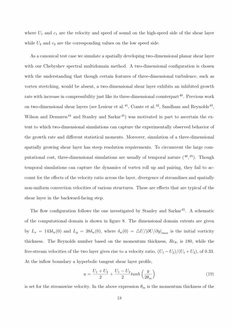
The flow configuration follows the one investigated by Stanley and Sarkar45. A schematic
of the computational domain is shown in figure 8. The dimensional domain extents are given
by Lx = 143δw(0) and Ly = 38δw(0), where δw(0) = 4U/|∂U/∂y|max is the initial vorticity
thickness. The Reynolds number based on the momentum thickness, Reθ, is 180, while the
free-stream velocities of the two layer gives rise to a velocity ratio, (U1−U2)/(U1 + U2), of 0.33.
At the inflow boundary a hyperbolic tangent shear layer profile,
u =U1 + U2
2+
U1 − U2
2tanh
(y
2θm
)(19)
is set for the streamwise velocity. In the above expression θm is the momentum thickness of the
18
shear layer, while U1 and U2 are the velocities of the high and low-speed streams, respectively.
The lateral velocity is taken as zero. Density and temperature are set to their uniform free-
stream values. The streamwise velocity at the top and bottom is set to U1 and U2, respectively.
The inflow values for the primitive variables are applied at the outflow boundary. The flow is
initialized with the hyperbolic-tangent profile (equation 19) for the streamwise velocity, while
density and temperature is taken to be their free-stream values.
In-order to investigate the effect of compressibility, we simulate three cases having Mach
number, Ma = 0.25, 0.5, 0.6. The lowest Mach number case is the “naturally developing” case
in Stanley and Sarkar45. The number of sub-domains employed in the x and y co-ordinate
directions are 32 and 8, respectively, while a polynomial of 7 is used within each sub-domain.
This gives a total of 20,736 Lobatto grid points.
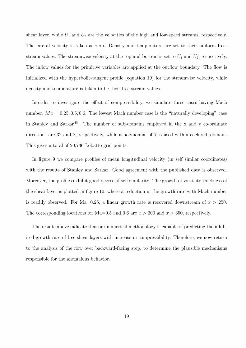
In figure 9 we compare profiles of mean longitudinal velocity (in self similar coordinates)
with the results of Stanley and Sarkar. Good agreement with the published data is observed.
Moreover, the profiles exhibit good degree of self similarity. The growth of vorticity thickness of
the shear layer is plotted in figure 10, where a reduction in the growth rate with Mach number
is readily observed. For Ma=0.25, a linear growth rate is recovered downstream of x > 250.
The corresponding locations for Ma=0.5 and 0.6 are x > 300 and x > 350, respectively.
The results above indicate that our numerical methodology is capable of predicting the inhib-
ited growth rate of free shear layers with increase in compressibility. Therefore, we now return
to the analysis of the flow over backward-facing step, to determine the plausible mechanisms
responsible for the anomalous behavior.
19

7.2 Role of convective Mach number and density ratio
The influence of the free-stream Mach number could manifest on the flow through the change in
convective Mach number and density ratio of the separated shear layer. For the developing shear
layer over the backward-facing step, prescription of U2 and c2 in equation 18, is non-trivial, due
to inhomogeneity in the streamwise direction and the presence of the recirculating region having
negative velocities. From figure 3 we observe that the magnitude of the negative velocities within
the recirculation bubble are small compared to to the free-stream flow. Hence, the separated
shear layer can be considered as a single stream shear layer and the convective Mach number is
determined with U2 ≈ 0. The speed of sound for the low speed stream is calculated based on
the minimum pressure and density, for a given streamwise location. This gives Mac=0.1, 0.15
and 0.2 for Ma2, Ma3 and Ma4, respectively. The above values indicate that the convective
Mach numbers for all three cases is in the quasi-incompressible regime25 and below the critical
value of 0.5 above which significant reduction in growth rate with the convective Mach number
is observed for canonical free shear flows. Therefore, compressibility effects owing to increase in
convective Mach number is expected to be minimal for the present study. Moreover, even if the
convective Mach number were to affect the shear layer development, an increase in its value would
result in slower growth rate, as observed in section 7.1, and consequently a longer reattachment
length. Thus, the increase in convective Mach number does not explain the observed shorter
reattachment for higher free-stream Mach numbers. Clearly, the developing compressible shear
layer in a backward-facing step flow does not follow the trend exhibited by simple free shear
layers.
Next, we investigate the mean density ratio that could influence the development of the shear
layer. Brown and Roshko47 studied the effect of the density ratio across a coflowing shear layer
20
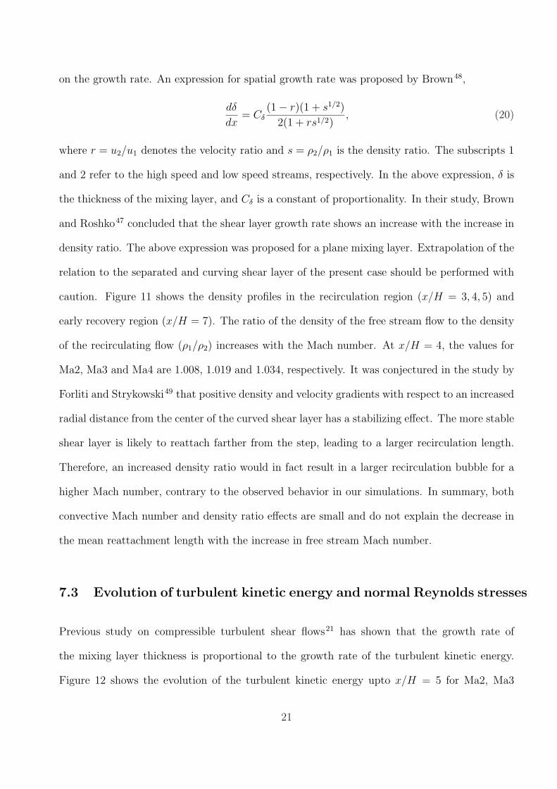
on the growth rate. An expression for spatial growth rate was proposed by Brown48,
dδ
dx= Cδ
(1− r)(1 + s1/2)
2(1 + rs1/2), (20)
where r = u2/u1 denotes the velocity ratio and s = ρ2/ρ1 is the density ratio. The subscripts 1
and 2 refer to the high speed and low speed streams, respectively. In the above expression, δ is
the thickness of the mixing layer, and Cδ is a constant of proportionality. In their study, Brown
and Roshko47 concluded that the shear layer growth rate shows an increase with the increase in
density ratio. The above expression was proposed for a plane mixing layer. Extrapolation of the
relation to the separated and curving shear layer of the present case should be performed with
caution. Figure 11 shows the density profiles in the recirculation region (x/H = 3, 4, 5) and
early recovery region (x/H = 7). The ratio of the density of the free stream flow to the density
of the recirculating flow (ρ1/ρ2) increases with the Mach number. At x/H = 4, the values for
Ma2, Ma3 and Ma4 are 1.008, 1.019 and 1.034, respectively. It was conjectured in the study by
Forliti and Strykowski49 that positive density and velocity gradients with respect to an increased
radial distance from the center of the curved shear layer has a stabilizing effect. The more stable
shear layer is likely to reattach farther from the step, leading to a larger recirculation length.
Therefore, an increased density ratio would in fact result in a larger recirculation bubble for a
higher Mach number, contrary to the observed behavior in our simulations. In summary, both
convective Mach number and density ratio effects are small and do not explain the decrease in
the mean reattachment length with the increase in free stream Mach number.
7.3 Evolution of turbulent kinetic energy and normal Reynolds stresses
Previous study on compressible turbulent shear flows21 has shown that the growth rate of
the mixing layer thickness is proportional to the growth rate of the turbulent kinetic energy.
Figure 12 shows the evolution of the turbulent kinetic energy upto x/H = 5 for Ma2, Ma3
21

and Ma4. Comparison of the three cases reveals that the spatial growth rate increases with
the increase in the free-stream Mach number. Ma2 has significantly lower turbulent kinetic
energy for x/H ≤ 4.5 compared to Ma3 and Ma4. At x/H = 3, Ma4 has a peak value of
0.05 while the peak for Ma2 is only ∼ 0.0125 (75% lower). The difference between Ma3 and
Ma4 is less significant. The increase in turbulent kinetic energy with Mach number for all
locations, x/H ≤ 4.5, implies that the separated shear layer goes into transition earlier and
thereafter grows faster as the free-stream Mach number is increased. The profiles also indicate
that for all cases, as the shear layer develops the location of the peak shifts closer to the bottom
wall, indicating curving of the shear layer. Cross-stream integrated kinetic energy for the same
locations is plotted in figure 13. The figure again underscores that upto x/H = 4.5, the growth
rate increases with Mach number. For Ma3 and Ma4 the integrated turbulent kinetic energy
shows a slight decrease after x/H = 4.5. Therefore, a faster streamwise growth of turbulent
kinetic energy explains why the shear layer grows faster and reattaches earlier with increase in
Mach number, resulting in a shorter mean reattachment length.
Evolution of the peak normal stresses, shown in figure 14, indicates that the streamwise
normal stress, {uu}, is the largest component for all the cases. The streamwise evolution,
however, is similar for all the components. All the stress components increase till approximately
one step-height from the reattachment point followed by a gradual reduction as the shear layer
starts to reattach. Subsequently, in the recovery region the stresses show a rapid decay. This is
unlike the compressible mixing layer past an axisymmetric trailing edge, investigated recently
by Simon et al.28. A distinctly different evolution for streamwise and wall normal stresses was
observed in the above study. Comparison of the different cases in figure 14 shows that there
is an increase in the magnitude of the stresses with the increase in Mach number, during the
development of the shear layer. Consistent with the faster growth of the shear layer, the normal
stresses increase rapidly for Ma3 and Ma4, compared to Ma2. However, as the shear layer relaxes
22

after reattachment the decay of the stresses are identical for the different Mach numbers.
The structural changes of turbulence in shear flows are often investigated by looking into
Reynolds stress anisotropy22;28,
bij =Rij − (2/3)kδij
2k, (21)
where Rij and k are the Reynolds stress and turbulent kinetic energy, respectively. The normal
stress anisotropy is shown in figure 15 at x/H = 4. The anisotropy of streamwise, {uu}, and
wall normal, {ww}, stresses is larger in the region close to the wall. Whereas, the spanwise
stress, {vv}, exhibits more anisotropy in the shear layer region, z/H > 1. On the low-speed side
of the shear layer and in the backflow region (0.125 < z/H < 0.75), the anisotropy in all three
stress components increases with the increase in Mach number. The maximum absolute values
in the region 0.125 < z/H < 0.75 for buu, bvv and bww are 0.16, 0.11 and 0.12, respectively for
Ma2. The corresponding values for Ma3 are 0.05, 0.07 and 0.08, while for Ma4 they are 0.03,
0.05 and 0.07.
7.4 Budget of turbulent kinetic energy: production
The observed difference in the growth rate of the turbulent kinetic energy can be explained by
computing the turbulent kinetic energy budget. In order to derive the transport equation for
turbulent kinetic energy, the Favre decomposition is applied to the convective terms, so that
they reduce to the same form as in the incompressible case. For all the other terms, we apply
the Reynolds decomposition. The derivation technique follows the work of Huang et al.50 and
results in an equation containing a mix of Favre-averaged (curly brackets) and Reynolds-averaged
(angled brackets) quantities,
∂〈ρ〉{uk}{k}∂xk
= −〈ρ〉{u′′i u′′k}∂{ui}∂xk
− ∂〈ρ〉{u′′kk′′}∂xk
− ∂〈p′u′k〉∂xk
23

+∂〈τ ′iku′i〉
∂xk
−⟨
τ ′ik∂u′i∂xk
⟩− 〈u′′k〉
∂〈p〉∂xk
+ 〈u′′i 〉∂〈τik〉∂xk
+
⟨p′
∂u′k∂xk
⟩, (22)
The first term on the right-hand side (RHS) of Eq. (22) represents the energy production;
the second, turbulent diffusion; the third, diffusion resulting from velocity-pressure interaction;
the fourth, viscous diffusion; the fifth, energy dissipation; and the last three are compressibility
related terms, the last one being the pressure dilatation. We demonstrate the accuracy of the
budget calculation, by plotting the left-hand side (LHS) and the RHS of the above equation at
two different streamwise locations. Figure 16 shows that our simulation leads to a good balance
between the two sides of Eq. (22).
Vreman et al.22 showed that the growth rate of a temporal mixing layer is proportional to the
integrated turbulence production. The growth rate of the momentum thickness (δ) was given
by,
dδ
dt= − 2
ρ∞(4U)2
∫ ({ρuw}∂U
∂z
)dz, (23)
where the term within the paranthesis is the turbulence production term. Moreover, the growth
rate of a self-similar spatial mixing layer was shown to be related to the temporal rate in a
transformed co-ordinate. Analysis of the data from the above study revealed that decreased
turbulent production was responsible for the reduced thickness of the shear layer with increase
in Mach number. Vreman et al.22 argued that the reduction in turbulence production with
increase in compressibility was linked to reduced pressure fluctuations via the reduction in the
pressure-strain term. The profiles of turbulent production in the recirculation zone are presented
in figure 17. It is seen that the production increases with the increase in Mach number upto
x/H = 3.5. At x/H = 4 and x/H = 4.5 cases Ma3 and Ma4 have similar profiles, while the
values are still lower for Ma2. An opposite trend with change in Mach number is observed at
x/H = 5.
As the shear layer impinges on the bottom wall in the reattachment region, the vortical
24

structures break up and this leads to a decrease in turbulence production. This is evident in
figure 18, which shows the production at two locations in the reattachment region. We notice
a considerable reduction in production, especially at x/H = 6.5, over that in the recirculation
region. The decrease also explains why a different trend is observed at x/H = 5 (figure 17) as
compared to locations upstream. Since, x/H = 5 is close to the reattachment point for Ma3
and Ma4, the production begins to decay, unlike in Ma2 where it continues to grow, relative to
the locations upstream.
Figure 19 shows the streamwise evolution of the cross-stream integrated turbulence produc-
tion for the three cases. Generally, upto x/H = 4.5, the integrated production shows an increase
with increase in the Mach number. For Ma4 a larger growth rate, compared to Ma2 and Ma3,
is observed upto x/H = 3.5 after which the growth is more gradual. Ma3 similarly exhibits
a higher growth than Ma2 till x/H = 4. This difference in growth of production with Mach
number can be possibly explained by looking at the Reynolds stress component, {uw}, which in
combination with the velocity gradient, ∂U/∂z, is the most significant production term. Profiles
of {uw} and the production at different streamwise locations are shown in figure 20 for Ma2 and
Ma4. The profiles indicate a strong spatial correlation between {uw} and production: the peak
location of production corresponds to the peak location of {uw}. Comparison of the shear stress
profiles for the three cases reveals that the stress increases with increase in the Mach number,
causing the larger production of turbulence thereof. Figure 21 shows the streamwise evolution
of cross-stream integrated shear stress. The plot indicates that upto x/H = 4.5 the integrated
values of shear stress, {uw}, scales with the Mach number.
25

7.5 Budget of turbulent kinetic energy: dissipation and pressure
dilatation
Dilatational dissipation and pressure dilatation are sink terms in the turbulent kinetic energy
equation that can be directly related to compressibility. When fluctuations in viscosity are
neglected, the total dissipation can be decomposed into solenoidal, εs, dilatational, εd, and
inhomogeneous, εI , terms
ε = εs + εd + εI , (24)
where
εs =2
Re〈ω′ijω′ij〉, (25)
εd =4
3
1
Re
⟨∂u′l∂xl
∂u′k∂xk
⟩, (26)
εI =2
Re
(∂2〈u′iu′j〉∂xi∂xj
− 2∂
∂xi
⟨u′i
∂u′j∂xj
⟩). (27)
Previous studies on compressible mixing layers22;25 showed that the dilatational part of the
dissipation was negligibly small and the pressure-dilatation, though not insignificant, was still
small compared to the total dissipation. Neither quantity was used to explain the observed
variation of shear layer growth rate with compressibility. Figures 22 and 23, respectively, show
the solenoidal and dilatational dissipation for the three cases in the recirculation zone. Com-
parison of the two figures reveals that the dilatational dissipation is two orders of magnitude
lower than the solenoidal dissipation for Ma3 and Ma4 and three orders of magnitude lower
for Ma2, and therefore has a negligible contribution to the turbulent kinetic energy budget.
An increase of dilatational dissipation with Mach number is the result of the increase in the
dilatation term (∂u‘k/∂xk) with compressibility. Solenoidal dissipation is therefore the primary
dissipation mechanism in the flow and as seen in figure 22, it is also strongly dependent on
the Mach number, especially in the early stages of shear layer development. Till x/H = 4, εs
26

increases with the increase in the Mach number. Ma2 has significantly lower dissipation than
Ma3 and Ma4. At x/H = 5, the values decrease with increase in the Mach number.
In compressible shear flows the dilatational dissipation is associated with the acoustic and the
entropy mode, while the solenoidal dissipation is associated with the vortical mode51. Thus, the
influence of Mach number on the solenoidal dissipation is expected to be small. The counter-
intuitive results observed in figure 22 therefore warrants some explanation. Budget of solenoidal
dissipation for compressible temporal mixing layers was computed by Kreuzinger et al.52 The
exact transport equation for solenoidal dissipation in compressible flow was considered in their
study. Two configurations, namely, channel flow and mixing layer were studied and the effects
of convective Mach number and mean density variation were investigated. The results indicated
that a change in Mach number did alter the budget of the solenoidal dissipation. However, the
authors concluded that compressibility effects in the transport equation for εs was of indirect
nature. The terms explicitly dependent on compressibility were small for all the cases studied,
except low Mach number mixing layer with large density variation. They argued that the
compressibility effects are proportional to the turbulent Mach number (urms/c) and the gradient
Mach number, both of which are related to the large scales of the flow, and not to the small
scales that determine the dissipation rate, thus explaining the indirect nature of the dependence.
The inhomogenous dissipation, εI , has negligible contribution to the turbulent kinetic energy
budget and therefore is not shown here.
Figure 24 shows the pressure dilatation in the recirculation region. Unlike dilatational dissi-
pation, pressure dilatation is comparable to the solenoidal dissipation (figure 22). As the shear
layer develops, the quantity increases upto locations close to the reattachment point. Thus for
Ma3 and Ma4 the increase is observed upto x/H = 4.5, while for Ma2 the growth is sustained till
x/H = 5. Similarly to dissipation, pressure dilatation is also strongly dependent on the Mach
number. Ma3 and Ma4 have significantly larger values compared to Ma2, the values being one
27

order of magnitude higher at locations close to the step (x/H ≤ 3.5). However, downstream of
x/H = 3.5, there is a large increase for Ma2 resulting in values comparable to the higher Mach
number cases. Thus even at the lowest Mach number studied, explicit effects of compressibility
via pressure-dilatation is non-negligible. This creates a fundamental physical difference between
our compressible flow simulation with the incompressible flow experiment of WHBJ. The dis-
crepancies between the experiment and Ma2, seen in section 5 can now be interpreted in the
light of the above finding.
As the shear layer reattaches, the pressure-dilatation becomes less sensitive to Mach number
change, as seen in figure 25. The solenoidal dissipation on the other hand has higher values
for lower Mach numbers, a trend that was observed earlier in figure 22(f). Such change in the
dependence of solenoidal dissipation on the Mach number indicates that the decay in dissipation
near the reattachment point is more pronounced when compressibility effects are larger.
7.6 Budget of turbulent kinetic energy: turbulent transport quanti-
ties
Turbulent diffusion in the recirculation and reattachment regions is plotted in figure 26. We
observe that the cross-stream profiles have distinct crest and trough. The negative values at the
bottom half of the shear layer indicate that energy is removed from the region, and transported
to the near wall region and to the top half of the shear layer. Comparison of the profiles at
different stations for the three cases, indicates that as the shear layer grows, the region over which
turbulent diffusion occurs widens in the cross-stream direction. At locations, x/H = 3.5 and
4.0, Ma3 and Ma4 have more turbulent transport, than does Ma2. Thereafter, the dependence
on Mach number is weak. The reattachment of the shear layer is accompanied by a reduction
in the turbulent transport (figure 26 (e), (f)).
28

Figure 27 shows the diffusion due to pressure-velocity correlation, in the recirculation and
reattachment regions. In turbulence modeling of compressible flow, the usual practice is to
neglect the pressure diffusion term53. The results here indicate that the magnitude of the term
is comparable to turbulent diffusion transport, and therefore its omission from modeling can
lead to significant error. Unlike turbulent diffusion, pressure diffusion is mostly negative across
the shear layer in the recirculation region (figure 27 (a)-(d)). Moreover, though the region
over which it has significant contribution to the turbulent kinetic energy budget increases with
streamwise distance, the peak value drops. In the reattachment region (x/H=5.5) (figure 27
(e)) there is a change from negative diffusion to positive diffusion.
The remaining terms in Eq. (22), namely, viscous diffusion (term 4), term 6 and term 7
have negligible contributions to the turbulent kinetic energy budget of the flow. Analysis of the
production, sink and transport terms, established production as the single largest contributor
to the budget. The growth of the shear layer and turbulent kinetic energy is therefore strongly
dependent on the production. As a result, higher production closer to the step with the increase
in Mach number leads to a faster development of the shear layer, which consequently reattaches
early and therefore leads to a shorter recirculation vortex.
8 Conclusions
We have investigated compressible flow over a backward-facing step using direct numerical sim-
ulation. In the absence of any compressible flow experiment at low Reynolds numbers (feasible
for DNS), we compare our results with the incompressible experiment of Wengle et al.12. Both
averaged flow and turbulent stresses are found to be sensitive to the free-stream Mach number.
The mean reattachment length decreases with increase in Mach number.
The complex topology of the flow in visualized using pressure iso-contours and helicity. As the
29

upstream laminar boundary layer undergoes transition after separation, Kelvin-Helmhotz billows
appear approximately 3-step heights from the step edge. These structures though nominally
two-dimensional, show waviness in the spanwise direction. Helicity is utilized to determine the
extent of “cockscrew” type motion present in the flow. Clustering of helical structures or vortex
cores within the shear layer indicates a strong “cockscrew” type motion. Subsequent reduction
in density of vortex cores with shear layer reattachment, implies breakdown of the coherent
structures upon impact with the wall.
The decrease in the mean reattachment length with compressibility implies that the separated
shear layer is less stable or grows faster for higher Mach numbers. This behavior is very different
from classical free-shear layers, where compressibility inhibits growth rate. As an aside, we
conduct simulation of a two-dimensional shear layer for different Mach numbers to establish
that our methodology is able to predict the above classical nature of compressible mixing layers.
Finally, we analyze in detail the effect of compressibility on the backward-facing step geome-
try. Effect of convective Mach number and the density ratio are small and does not explain the
anomalous behavior. Growth of mixing layers is linked to evolution of turbulent kinetic energy.
A larger growth in turbulent kinetic energy with Mach number therefore explains the faster
spread of the shear layer. The full budget of turbulent kinetic energy is computed to determine
the effect of compressibility on each of the budget terms. Production is the most significant
term in the budget, which increases with Mach number, thereby resulting in faster growth of
turbulent kinetic energy. Further analysis reveals that the shear stress, {uw}, is responsible
for larger production with increase in compressibility. In the turbulent kinetic energy budget,
dilatational dissipation and pressure dilatation are the terms directly related to compressibility
(dilatation). As in case of canonical mixing layers, dilatational dissipation is negligibly small
for the backward-facing step flow. The primary dissipation therefore comes from the solenoidal
velocity field. Pressure dilatation however, is comparable to the total dissipation, unlike in
30

the canonical free-shear flows investigated before. Among the transport terms, only turbulent
diffusion and diffusion due to velocity-pressure correlation have significant contribution to the
budget. RANS modeling for compressible flows usually neglects the transport due to pressure-
velocity correlation. Our results therefore, underscores that such an omission could lead to large
errors. Turbulent diffusion transports energy from the bottom half of the shear layer to the near
wall and upper half of the shear layer.
The analysis and conclusions presented in this paper establish that the compressible shear
layer over backward-facing step is distinct in its response to increase in compressibility. The
findings can be useful in the design of combustors, flame-holders in high-speed propulsion which
are often modeled after the backward-facing step geometry.
31

References
[1] J. K. Eaton and J. P. Johnston. Turbulent flow reattachment: A experimental study of
the flow structure behind a backward facing step. Report, Thermosciences Division, Dept.
Mechanical Engineering MD-39, Stanford University, 1980.
[2] B. F. Armaly, F. Durst, J. C. F. Peireira, and B. Schonung. Experimental and theoretical
inspection of backward-facing step flow. Journal of Fluid Mechanics, 127:473–496, 1983.
[3] F. Durst and C. Tropea. In Proceedings of 3rd Intl. Symp. on Turbulent Shear Flows,
page 18, Davis, CA.
[4] E. W. Adams, J. P. Johnston, and J. K. Eaton. Experiments on the structure of turbulent
reattaching flows. Report, Thermosciences Division, Dept. Mechanical Engineering MD-43,
Stanford University, 1984.
[5] K. Ishomoto and S. Honami. The effect of inlet turbulence intensity on the reattachment
preocess over a backward-facing step. ASME Journal of Fluids Engg, 111:87–92, 1989.
[6] J. Kim and P. Moin. Application of a fractional step method to incompressible Navier-
Stokes equations. Journal of Comput. Physics, 59:308–323, 1985.
[7] L. Kaikatis, G. E Karniadakis, and S. A. Orszag. Onset of tree dimensionality, equilibria,
and early transition in flow over a backward-facing step. Journal of Fluid Mechanics,
231:501–528, 1991.
[8] L. Kaikatis, G. E Karniadakis, and S. A. Orszag. Unsteadiness and convective instabilities in
a two-dimensional flow over a backward-facing step. Journal of Fluid Mechanics, 321:157–
187, 1996.
[9] H. Le, P. Moin, and J. Kim. Direct numerical simulation of turbulent flow over a backward-
facing step. Journal of Fluid Mechanics, 330:349–374, 1997.
32

[10] S. Jovic and D. M. Driver. Backward-facing step measurement at low reynolds number,
reh=5000. NASA Tech. Mem. 108807, NASA, 1994.
[11] H. J. Kaltenbach and G. Janke. Direct numerical simulation of flow separation behind a
rearward-facing step at Re=3000. Physics of Fluids, 12:2320–2337.
[12] H. Wengle, A. Huppertz, G. Barwolff, and G. Janke. The manipulated transitional
backward-facing step flow: An experimental and direct numerical simulation investigation.
Eur. J. Mech. B - Fluids, 20:25–46, 2001.
[13] D. Barkley, M. G. M. Gomes, and R. D. Henderson. Three-dimensional instability in flow
over a backward-facing step. Journal of Fluid Mechanics, 473:167–190, 2002.
[14] S. K. Lele. Compressibility effects on turbulence. Annual Reviews in Fluid Mechanics,
26:211–254, 1994.
[15] D. Bogdanoff. Compressibility effects in turbulent shear layers. AIAA J, 21:926–927, 1983.
[16] D. Papamoschou and A. Roshko. The compressible turbulent shear layer: An experimental
study. J. Fluid Mech., 197:453–477, 1988.
[17] J. L. Hall, P. E. Dimotakis, and H. Rosemann. Experiments in non-reacting compressible
shear layers. AIAA J., 31:2247–2254, 1993.
[18] J. L. Hall, P. E. Dimotakis, and H. Rosemann. Large-scale structure and entrainment in
the supersonic mixing layer. Journal of Fluid Mechanics, 284:171–216, 1995.
[19] O. Zeman. Dilatational dissipation-the concept and application in modeling compressible
mixing layers. Phys. Fluids, 2:178–188, 1990.
[20] S. Sarkar. The pressure-dilatation correlation in compressible flows. Phys. Fluids,
4(12):2674–2682, 1992.
33

[21] S. Sarkar. The stabilizing effect of compressibility in turbulent shear flow. Journal of Fluid
Mechanics, 282:163–186, 1995.
[22] A. W. Vreman, N. D. Sandham, and K. H. Luo. Compressible mixing layer growth rate
and turbulence characteristics. Journal of Fluid Mechanics, 320:235–258, 1996.
[23] S. Sarkar. On density and pressure fluctuations in uniformly sheared compressible flow. In
IUTAM Symp. on Variable Density Low-Speed Flows, Marseille, France, 1996.
[24] J. B. Freund, S. K. Lele, and P. Moin. Compressibility effects in a turbulent annular mixing
layer. part 1. Turbulence and growth rate. Journal of Fluid Mechanics, 421:229–267, 2000.
[25] C. Pantano and S. Sarkar. A study of compressibility effects in the high-speed turbulent
shear layer using direct simulation. Journal of Fluid Mechanics, 451:329–371, 2002.
[26] R. V. R. Avancha and R. H. Pletcher. Large-eddy simulation of the turbulent flow past
a backward-facing step with heat transfer nd property variation. International Journal of
Heat and Fluid Flow, 23:601–614, 2002.
[27] J. Dandois, E. Garnier, and P. Sagaut. Numerial simulation of active separation control by
a synthetic jet. Journal of Fluid Mech., 574:25–58, 2007.
[28] F. Simon, S. Deck, P. Gullien, P. Sagaut, and A. Merlen. Numerial simulation of the
compressible mixing layer past an axisymmetric trailing edge. Journal of Fluid Mech.,
591:215–253, 2007.
[29] G. A. Bres and T. Colonius. Three-dimensional instabilities in compressible flow over
cavities. Journal of Fluid Mech., 599:309–339, 2008.
[30] G. B. Jacobs, D. A. Kopriva, and F. Mashayek. Validation study of a multidomain spectral
code for simulation of turbulent flows. AIAA Journal, 43(6):1256–1264, 2005.
34

[31] G. B. Jacobs, D. A. Kopriva, and F. Mashayek. A conservative isothermal wall boundary
condition for the compressible Navier-Stokes equation. Journal of Scientific Computing,
30(2):177–192, 2007.
[32] K. Sengupta, G. B. Jacobs, and F. Mashayek. Large-eddy simulation of compressible flows
using a spectral multidomain method. International Journal for Numerical Methods in
Fluids.
[33] P. L. Roe. Approximate Riemann solvers, parameter vectors, and difference schemes. J.
Comp. Phys., 43:357–372, 1981.
[34] D. A. Kopriva and J. H. Kolias. A conservative staggared-grid Chebyshev multidomain
method for compressible flows. Journal of Comput. Physics, 125:244–261, 1996.
[35] G. B. Jacobs, D. A. Kopriva, and F. Mashayek. A comparison of outflow boundary condi-
tions for the multidomain staggered-grid spectral method. Numer. Heat Transfer, Part B,
44(3):225–251, 2003.
[36] A. S. Neto, D. Grand, O. Metais, and M. Lesieur. A numerical investigation of the coherent
vortices in turbulence behind a backward-facing step. Journal of Fluid Mechanics, 256:1–25,
1993.
[37] G. E. M. Karniadakis and S. Sherwin. Spectral/hp Element Methods for Computational
Fluid Dynamics. Oxford University Press, New York, USA, 2005.
[38] G. B. Jacobs. Numerical Simulation of Two-Phase Turbulent Compressible Flows With A
Multidomain Spectral Method. Ph.D. Thesis, University of Illinois at Chicago, Chicago, IL,
2003.
[39] H. K. Moffatt and A. Tsinober. Helicity in laminar and turbulent flow. Annual Review of
Fluid Mechanics, 24:281–312, 1992.
35

[40] M. Lesieur. Turbulence in Fluids. Kluwer Academic Publisher, Dordrecht, Netherlands,
1990.
[41] M. Lesieur, C Staquet, P. L. Roy, and P. Comte. Mixing layer and its coherence examined
from the point of view of two-dimensional turbulence. Journal of Fluid Mechanics, 192:511–
534, 1988.
[42] P. Comte, M. Lesieur, H. Laroche, and X. Normand. In In Turbulent Shear Flows 6, page
361, Berlin.
[43] N. D. Sandham and W. C. Reynolds. In In Turbulent Shear Flows 6, page 441, Berlin.
[44] R. V. Wilson and A. O. Demuren. Numerical simulation of two-dimensional spatially
developing mixing layers. Icase Report 94-32, Institute for Computer Application in Science
and Engineering, NASA Langley Research Center, Hampton, VA, 1994.
[45] S. Stanley and S. Sarkar. Simulations of spatially developing two-dimensional shear layers
and jets. Theoretical Comput. Fluid Dynamics, 9:121–147, 1997.
[46] M. M. Rogers and R. D. Moser. Direct simulation of self-similar turbulent mixing layer.
Physics of Fluids, 6:903–923.
[47] G. L. Brown and A. Roshko. On density effects and large structure in turbulent mixing
layers. J. Fluid Mech., 64:775–816, 1974.
[48] G. Brown. The entrainment and large structure in turbulent mixing layers. In 5th Aus-
tralasian Conf. on Hydraulics and Fluid Mechanics, Canterbury, 1974. Canterbury Univer-
sity.
[49] D. J. Forliti and P. J. Strykowski. An overview of the turbulent shear layer: mixing
processes in propulsion systems. Internal report, dept. mechanical engineering, University
of Minnesota, 2003.
36

[50] P. G. Huang, G. N. Coleman, and P. Bradshaw. Compressible turbulent channel flows: Dns
results and modelling. Journal of Fluid Mechanics, 305:185–218, 1995.
[51] A. J. Smits and J-P. Dussage. Turbulent Shear Layers in Supersonic Flow. Springer,
Springer, 2006.
[52] J. Kreuzinger, R. Friedrich, and T. B. Gatski. A compressibility effect in the solenoidal
dissipation rate equation: A priori analysis and modeling. International Journal of Heat
and Fluid Flow, 27:696–706, 2006.
[53] David C. Wilcox. Turbulence Modeling for CFD. DCW Industries, Inc., La Canada, CA,
1993.
37

List of Tables
1 Cases investigated for the compressible flow over backward-facing step. . . . . . 39
38
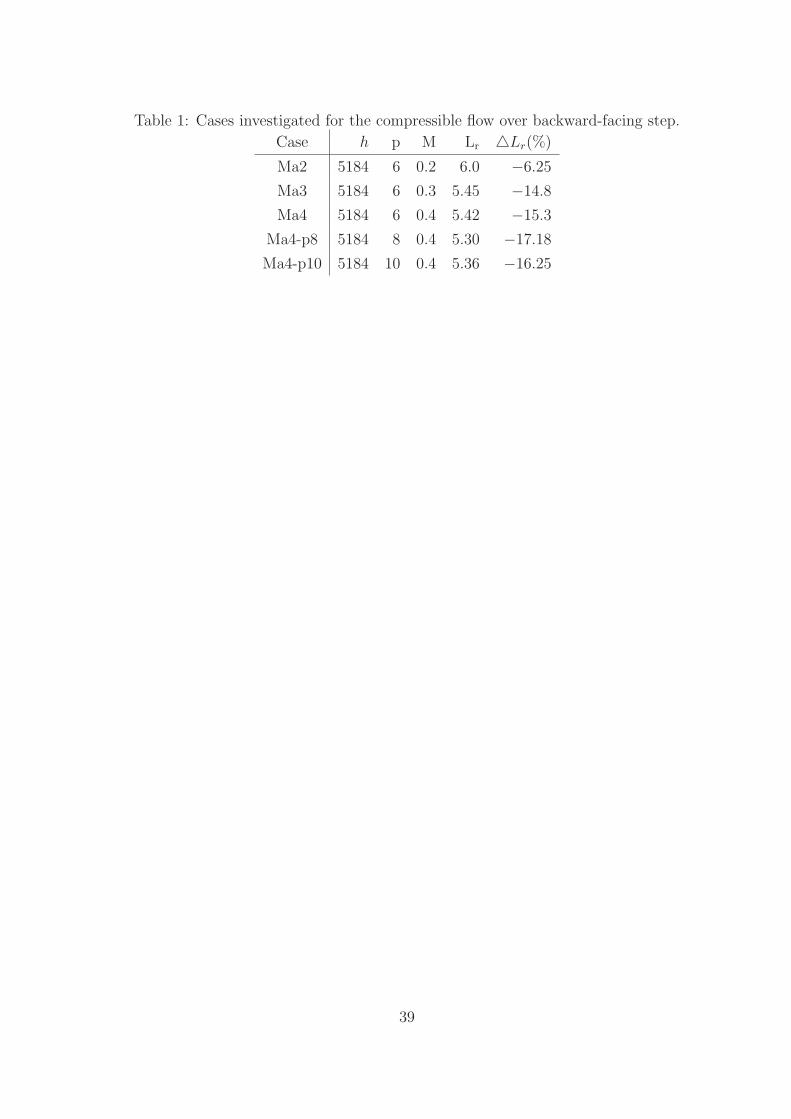
Table 1: Cases investigated for the compressible flow over backward-facing step.
Case h p M Lr 4Lr(%)
Ma2 5184 6 0.2 6.0 −6.25
Ma3 5184 6 0.3 5.45 −14.8
Ma4 5184 6 0.4 5.42 −15.3
Ma4-p8 5184 8 0.4 5.30 −17.18
Ma4-p10 5184 10 0.4 5.36 −16.25
39

List of Figures
1 Schematic of the backward-facing step configuration . . . . . . . . . . . . . . . . . . 42
2 Convergence study through comparison of averaged velocities. Streamwise velocity
(top), wall normal velocity (bottom) for Ma=0.4 for different polynomial approximation
orders. . . . . . . . . . . . . . . . . . . . . . . . . . . . . . . . . . . . . . . . . . 42
3 Comparison of averaged streamwise velocity (top), and wall normal velocity (bottom)
with the experiment of incompressible flow12. . . . . . . . . . . . . . . . . . . . . . 43
4 Convergence study through comparison of Favre averaged stresses for Ma=0.4 for dif-
ferent polynomial approximation orders. . . . . . . . . . . . . . . . . . . . . . . . . 43
5 Comparison of Favre averaged streamwise normal stress (top), and shear stress (bottom)
with the experiment of incompressible flow12. . . . . . . . . . . . . . . . . . . . . . 44
6 Pressure iso-contours indicating the flow topology for the case Ma4. . . . . . . . . . . 44
7 Vortex cores depicting the helical density in the flow for the case Ma4. . . . . . . . . 45
8 Schematic of the free shear layer configuration. . . . . . . . . . . . . . . . . . . . . 45
9 Mean streamwise velocity in self similar co-ordinates for two-dimensional free shear layer. 45
10 Growth of vorticity thickness of two-dimensional shear layer for different Mach numbers. 46
11 Averaged density plotted as a function of cross-streaam co-ordinate at (a) x/H=3, (b)
x/H=4, (c) x/H=5, (d) x/H=7. . . . . . . . . . . . . . . . . . . . . . . . . . . . . 46
12 Streamwise evolution of turbulent kinetic energy for (a) Ma2, (b) Ma3, (c) Ma4. . . . 47
13 Cross-stream integrated turbulent kinetic energy. . . . . . . . . . . . . . . . . . . . 47
14 Streamwise evolution of peak normal stresses. . . . . . . . . . . . . . . . . . . . . . 48
40

15 Anisotropy of normal stresses at x/H=4 for (a) Ma2, (b) Ma3 and (c) Ma4. . . . . . 48
16 Balance of turbulent kinetic energy budget for Ma4. . . . . . . . . . . . . . . . . . . 49
17 Production of turbulent kinetic energy: (a) x/H=2.5, (b) x/H=3.0, (c) x/H=3.5, (d)
x/H=4.0, (e) x/H=4.5, (f) x/H=5.0. . . . . . . . . . . . . . . . . . . . . . . . . . . 49
18 Production of turbulent kinetic energy in the reattachment region for (a) x/H=5.5 and
(b) x/H=6.5. . . . . . . . . . . . . . . . . . . . . . . . . . . . . . . . . . . . . . . 50
19 Cross-stream integrated production of turbulent kinetic energy. . . . . . . . . . . . . 51
20 Streamwise evolution of (a) shear stress, (b) production for Ma2 (top) and Ma4 (bottom). 51
21 Cross-stream integrated shear stress. . . . . . . . . . . . . . . . . . . . . . . . . . . 52
22 Solenoidal dissipation at (a) x/H=2.5, (b) x/H=3, (c) x/H=3.5, (d) x/H=4.0, (e)
x/H=4.5, (f) x/H=5. . . . . . . . . . . . . . . . . . . . . . . . . . . . . . . . . . . 53
23 Dilatational dissipation at (a) x/H=2.5, (b) x/H=3, (c) x/H=3.5, (d) x/H=4.0,(e)
x/H=4.5, (f) x/H=5. . . . . . . . . . . . . . . . . . . . . . . . . . . . . . . . . . . 54
24 Pressure dilatation at (a) x/H=2.5, (b) x/H=3, (c) x/H=3.5, (d) x/H=4.0, (e) x/H=4.5,
(f) x/H=5. . . . . . . . . . . . . . . . . . . . . . . . . . . . . . . . . . . . . . . . 54
25 Solenoidal dissipation (lines) and pressure dilatation (lines with symbols) in the reat-
tachment region for (a) x/H=5.5 and (b) x/H=6.5. . . . . . . . . . . . . . . . . . . 55
26 Turbulent diffusion of k at (a) x/H=3.5, (b) x/H=4.0, (c) x/H=4.5, (d) x/H=5, (e)
x/H=5.5, and (f) x/H=6.5. . . . . . . . . . . . . . . . . . . . . . . . . . . . . . . . 55
27 Pressure diffusion of k at (a) x/H=3.5, (b) x/H=4.0, (c) x/H=4.5, (d) x/H=5, (e)
x/H=5.5, and (f) x/H=6.5. . . . . . . . . . . . . . . . . . . . . . . . . . . . . . . . 56
41

5
6
1
X
ZY
17.92
10.76
Figure 1: Schematic of the backward-facing step configuration
0 0.5 1U
0
0.5
1
1.5
2
z/H
Exp.p=6p=8p=10
0 0.5 1U
0
0.5
1
1.5
2
0 0.5 1U
0
0.5
1
1.5
2
0 0.5 1U
0
0.5
1
1.5
2
-0.2 -0.1 0W
0
0.5
1
1.5
2
z/H
-0.2 -0.1 0W
0
0.5
1
1.5
2
-0.2 -0.1 0W
0
0.5
1
1.5
2
-0.2 -0.1 0W
0
0.5
1
1.5
2
x/H=7x/H=5x/H=4x/H=3
Figure 2: Convergence study through comparison of averaged velocities. Streamwise velocity (top),
wall normal velocity (bottom) for Ma=0.4 for different polynomial approximation orders.
42

0 0.5 1U
0
0.5
1
1.5
2
z/H
Exp.
Ma2Ma3Ma4
0 0.5 1U
0
0.5
1
1.5
2
0 0.5 1U
0
0.5
1
1.5
2
0 0.5 1U
0
0.5
1
1.5
2
-0.2 -0.1 0W
0
0.5
1
1.5
2
z/H
-0.2 -0.1 0W
0
0.5
1
1.5
2
-0.2 -0.1 0W
0
0.5
1
1.5
2
-0.1 -0.05 0W
0
0.5
1
1.5
2
x/H=3 x/H=4 x/H=5 x/H=7
Figure 3: Comparison of averaged streamwise velocity (top), and wall normal velocity (bottom) with
the experiment of incompressible flow12.
0 0.02 0.04 0.06 0.08{uu}
0
0.5
1
1.5
2
z/H
0 0.02 0.04 0.06{uu}
0
0.5
1
1.5
2
0 0.01 0.02 0.03{uu}
0
0.5
1
1.5
2
p=6p=8
0 0.01 0.02 0.03 0.04{uw}
0
0.5
1
1.5
2
z/H
0 0.01 0.02 0.03{uw}
0
0.5
1
1.5
2
0 0.01 0.02{uw}
0
0.5
1
1.5
2
x/H=4 x/H=6 x/H=8
Figure 4: Convergence study through comparison of Favre averaged stresses for Ma=0.4 for different
polynomial approximation orders.
43

0 0.04 0.08{uu}
0
0.5
1
1.5
2
z/H
Exp.Ma2Ma3Ma4
0 0.04 0.08{uu}
0
0.5
1
1.5
2
0 0.02 0.04{uu}
0
0.5
1
1.5
2
0 0.02 0.04{uw}
0
0.5
1
1.5
2
z/H
0 0.02 0.04{uw}
0
0.5
1
1.5
2
0 0.01 0.02{uw}
0
0.5
1
1.5
2
x/H=4 x/H=6 x/H=8
Figure 5: Comparison of Favre averaged streamwise normal stress (top), and shear stress (bottom)
with the experiment of incompressible flow12.
Figure 6: Pressure iso-contours indicating the flow topology for the case Ma4.
44

Figure 7: Vortex cores depicting the helical density in the flow for the case Ma4.
High speed side
Low speed side
Outflow
Mean flow direction
L x
InflowLy
x
y
Figure 8: Schematic of the free shear layer configuration.
-2 -1 0 1 2y/δ
w(x)
0
0.25
0.5
0.75
1
U-U
2
x*/d
w(0)=50, Ma=0.25
x*/d
w(0)=75, Ma=0.25
Stanley and Sarkar
Figure 9: Mean streamwise velocity in self similar co-ordinates for two-dimensional free shear layer.
45

0 100 200 300 400x
5
10
15
δ w(x
)
Ma=0.25Ma=0.5Ma=0.6
Figure 10: Growth of vorticity thickness of two-dimensional shear layer for different Mach numbers.
0.95 0.96 0.97 0.98 0.99 10
1
2
3
z/H
Ma2Ma3Ma4
0.96 0.98 10
1
2
3
0.98 0.99 1 ρ
0
1
2
3
z/H
0.99 1 1.01 1.02 ρ
0
1
2
3
(a) (b)
(c) (d)
Figure 11: Averaged density plotted as a function of cross-streaam co-ordinate at (a) x/H=3, (b)
x/H=4, (c) x/H=5, (d) x/H=7.
46

0 0.5 1 1.5 2z/H
0
0.05
0.1
k
0 0.5 1 1.5 2z/H
0
0.05
0.1
x/H=0.5x/H=1x/H=1.5x/H=2x/H=2.5x/H=3x/H=3.5x/H=4x/H=4.5x/H=5
0 0.5 1 1.5 2z/H
0
0.05
0.1
(a) (b) (c)
Figure 12: Streamwise evolution of turbulent kinetic energy for (a) Ma2, (b) Ma3, (c) Ma4.
0 1 2 3 4 5x/H
0
0.02
0.04
0.06
0.08
k (c
ross
-str
eam
inte
grat
ed)
Ma2Ma3Ma4
Figure 13: Cross-stream integrated turbulent kinetic energy.
47

2 3 4 5 6 7 80
0.04
0.08
{uu}
Ma2Ma3Ma4
2 3 4 5 6 7 80
0.04
0.08
{vv}
2 3 4 5 6 7 8x/H
0
0.04
0.08
{ww
}
Figure 14: Streamwise evolution of peak normal stresses.
0 0.5 1 1.5 2-0.4
-0.2
0
0.2
0.4
b ij
buu
bvv
bww
0 0.5 1 1.5 2-0.4
-0.2
0
0.2
0.4
b ij
0 0.5 1 1.5 2z/H
-0.4
-0.2
0
0.2
0.4
b ij
(a)
(b)
(c)
Figure 15: Anisotropy of normal stresses at x/H=4 for (a) Ma2, (b) Ma3 and (c) Ma4.
48

0.5 1 1.5 2
0
0.01
0.02
0.03
Bud
get
LHSRHS
0.5 1 1.5 2z/H
-0.02
-0.01
0
0.01
0.02
0.03
Bud
get
x/H=3.5
x/H=4
Figure 16: Balance of turbulent kinetic energy budget for Ma4.
0.5 1 1.5 20
0.02
0.04
0.06
0.08
Prod
uctio
n of
k
Ma2Ma3Ma4
0.5 1 1.5 20
0.02
0.04
0.06
0.08
0.5 1 1.5 20
0.02
0.04
0.06
0.08
0.5 1 1.5 2z/H
0
0.02
0.04
0.06
0.08
Prod
uctio
n of
k
0.5 1 1.5 2z/H
0
0.02
0.04
0.06
0.08
0.5 1 1.5 2z/H
0
0.02
0.04
0.06
0.08
(a) (b) (c)
(d) (e) (f)
Figure 17: Production of turbulent kinetic energy: (a) x/H=2.5, (b) x/H=3.0, (c) x/H=3.5, (d)
x/H=4.0, (e) x/H=4.5, (f) x/H=5.0.
49

0.5 1 1.5 20
0.02
0.04
0.06
Prod
uctio
n of
k Ma2Ma3Ma4
0.5 1 1.5 2z/H
0
0.01
0.02
0.03
Prod
uctio
n of
k
(a)
(b)
Figure 18: Production of turbulent kinetic energy in the reattachment region for (a) x/H=5.5 and (b)
x/H=6.5.
50

0 1 2 3 4 5x/H
0
0.005
0.01
0.015
0.02
0.025
0.03
Cro
ss-s
trea
m in
tegr
ated
pro
duct
ion
of k
Ma2Ma3Ma4
Figure 19: Cross-stream integrated production of turbulent kinetic energy.
0 0.5 1 1.5 2-0.04
-0.03
-0.02
-0.01
0
{uw
}
x/H=2.5x/H=3x/H=3.5x/H=4x/H=4.5
0.5 1 1.5 20
0.02
0.04
0.06
0.08
Prod
uctio
n of
k
0 0.5 1 1.5 2z/H
-0.04
-0.03
-0.02
-0.01
0
{uw
}
0.5 1 1.5 2z/H
0
0.02
0.04
0.06
0.08
Prod
uctio
n of
k
(a) (b)
(a) (b)
Figure 20: Streamwise evolution of (a) shear stress, (b) production for Ma2 (top) and Ma4 (bottom).
51

2 2.5 3 3.5 4 4.5 5x/H
0
0.01
0.02
0.03
Cro
ss-s
trea
m in
tegr
ated
{uw
}
Ma2Ma3Ma4
Figure 21: Cross-stream integrated shear stress.
52

0.5 1 1.5 20
0.002
0.004
0.006
ε s
0.5 1 1.5 20
0.005
0.01
0.015
0.5 1 1.5 20
0.01
0.02
0.03
Ma2Ma3Ma4
0.5 1 1.5 2
z/H
0
0.01
0.02
0.03
ε s
0.5 1 1.5 2
z/H
0
0.01
0.02
0.03
0.5 1 1.5 2
z/H
0
0.01
0.02
0.03
(a) (b) (c)
(d) (e) (f)
Figure 22: Solenoidal dissipation at (a) x/H=2.5, (b) x/H=3, (c) x/H=3.5, (d) x/H=4.0, (e) x/H=4.5,
(f) x/H=5.
53

0.5 1 1.5 20
5e-06
1e-05
1.5e-05
2e-05
ε d
0.5 1 1.5 20
1e-05
2e-05
3e-05
4e-05
5e-05
0.5 1 1.5 20
0.0001
0.0002Ma2Ma3Ma4
0.5 1 1.5 2
z/H
0
0.0001
0.0002
ε d
0.5 1 1.5 2
z/H
0
0.0001
0.0002
0.5 1 1.5 2
z/H
0
0.0001
0.0002
(a) (b) (c)
(d) (e) (f)
Figure 23: Dilatational dissipation at (a) x/H=2.5, (b) x/H=3, (c) x/H=3.5, (d) x/H=4.0,(e) x/H=4.5,
(f) x/H=5.
0.5 1 1.5 2-0.002
-0.0015
-0.001
-0.0005
0
Pres
sure
-dila
tatio
n
0.5 1 1.5 2-0.004
-0.003
-0.002
-0.001
0
0.5 1 1.5 2-0.008
-0.006
-0.004
-0.002
0
Ma2Ma3Ma4
0.5 1 1.5 2
z/H
-0.02
-0.015
-0.01
-0.005
0
Pres
sure
-dila
tatio
n
0.5 1 1.5 2
z/H
-0.02
-0.015
-0.01
-0.005
0
0 0.5 1 1.5 2
z/H
-0.02
-0.015
-0.01
-0.005
0
(a) (b) (c)
(d) (e) (f)
Figure 24: Pressure dilatation at (a) x/H=2.5, (b) x/H=3, (c) x/H=3.5, (d) x/H=4.0, (e) x/H=4.5,
(f) x/H=5.
54

0.5 1 1.5 2-0.02
0
0.02
0.04
ε s, p-d
ilata
tion Ma2
Ma3Ma4
0.5 1 1.5 2z/H
-0.01
0
0.01
0.02
ε s, p-d
ilata
tion
(a)
(b)
Figure 25: Solenoidal dissipation (lines) and pressure dilatation (lines with symbols) in the reattach-
ment region for (a) x/H=5.5 and (b) x/H=6.5.
0.5 1 1.5 2-0.04
-0.02
0
0.02
0.04
Tur
bule
nt d
iffu
sion
Ma2Ma3Ma4
0.5 1 1.5 2-0.04
-0.02
0
0.02
0.04
0.5 1 1.5 2-0.04
-0.02
0
0.02
0.04
0.5 1 1.5 2
z/H
-0.04
-0.02
0
0.02
0.04
Tur
bule
nt d
iffu
sion
0.5 1 1.5 2
z/H
-0.04
-0.02
0
0.02
0.04
0.5 1 1.5 2
z/H
-0.04
-0.02
0
0.02
0.04
(a) (b) (c)
(d) (e) (f)
Figure 26: Turbulent diffusion of k at (a) x/H=3.5, (b) x/H=4.0, (c) x/H=4.5, (d) x/H=5, (e)
x/H=5.5, and (f) x/H=6.5.
55

0.5 1 1.5 2-0.04
-0.02
0
0.02
0.04
Pres
sure
-dif
fusi
on
Ma2Ma3Ma4
0.5 1 1.5 2-0.04
-0.02
0
0.02
0.04
0.5 1 1.5 2-0.04
-0.02
0
0.02
0.04
0.5 1 1.5 2
z/H
-0.04
-0.02
0
0.02
0.04
Pres
sure
-dif
fusi
on
0.5 1 1.5 2
z/H
-0.04
-0.02
0
0.02
0.04
0.5 1 1.5 2
z/H
-0.04
-0.02
0
0.02
0.04
(a) (b) (c)
(d) (e) (f)
Figure 27: Pressure diffusion of k at (a) x/H=3.5, (b) x/H=4.0, (c) x/H=4.5, (d) x/H=5, (e) x/H=5.5,
and (f) x/H=6.5.
56