dirichlet-hawkes processes with applications to …lsong/papers/dufarahmsmoson15.pdf ·...
TRANSCRIPT

Dirichlet-Hawkes Processes with Applications toClustering Continuous-Time Document Streams
Nan DuGeorgiaTech
Atlanta, GA, [email protected]
Mehrdad FarajtabarGeorgiaTech
Atlanta, GA, [email protected]
Amr AhmedGoogle Strategic Technologies
Mountain View, CA, [email protected]
Alexander J. SmolaCarnegie Mellon University
Pittsburgh, PA, [email protected]
Le SongGeorgiaTech
Atlanta, GA, [email protected]
ABSTRACTClusters in document streams, such as online news articles,can be induced by their textual contents, as well as by thetemporal dynamics of their arriving patterns. Can we lever-age both sources of information to obtain a better clusteringof the documents, and distill information that is not possi-ble to extract using contents only? In this paper, we pro-pose a novel random process, referred to as the Dirichlet-Hawkes process, to take into account both information ina unified framework. A distinctive feature of the proposedmodel is that the preferential attachment of items to clustersaccording to cluster sizes, present in Dirichlet processes, isnow driven according to the intensities of cluster-wise self-exciting temporal point processes, the Hawkes processes.This new model establishes a previously unexplored connec-tion between Bayesian Nonparametrics and temporal PointProcesses, which makes the number of clusters grow to ac-commodate the increasing complexity of online streamingcontents, while at the same time adapts to the ever chang-ing dynamics of the respective continuous arrival time. Weconducted large-scale experiments on both synthetic andreal world news articles, and show that Dirichlet-Hawkesprocesses can recover both meaningful topics and temporaldynamics, which leads to better predictive performance interms of content perplexity and arrival time of future docu-ments.
Categories and Subject DescriptorsH.4 [Information Systems Applications]: Miscellaneous;D.2.8 [Software Engineering]: Metrics—complexity mea-sures, performance measures
KeywordsDirichlet Process, Hawkes Process, Document Modeling
Permission to make digital or hard copies of all or part of this work forpersonal or classroom use is granted without fee provided that copies arenot made or distributed for profit or commercial advantage and that copiesbear this notice and the full citation on the first page. To copy otherwise, torepublish, to post on servers or to redistribute to lists, requires prior specificpermission and/or a fee.KDD ’15 Sydney, NSW AustraliaCopyright 2015 ACM X-XXXXX-XX-X/XX/XX ...$15.00.
1. INTRODUCTIONOnline news articles, blogs and tweets tend to form clus-
ters around real life events and stories on certain topics [2,3, 9, 20, 7, 22]. Such data are generated by myriads of onlinemedia sites in real-time and in large volume. It is a criticallyimportant task to effectively organize these articles accord-ing to their contents such that online users can quickly siftand digest them.
Besides textual information, temporal information alsoprovides very good clue on the clustering of online documentstreams. For instance, weather reports, forecast and warningof the blizzard in New York city this year appeared onlineeven before the snowstorm actually begins1. As the bliz-zard conditions gradually intensify, more subsequent blogs,posts and tweets were triggered around this event in variousonline social media. Such self-excitation phenomenon oftenleads to many closely related articles within a short periodof time. Later, after the influence of the event passes itspeak, e.g., the blizzard eventually stopped, public attentiongradually turned to other events, and the number of articleson the blizzard faded out eventually.
Furthermore, depending on the nature of real life events,relevant news articles can exhibit very different temporaldynamics. For instance, articles on emergency or incidentsmay rise and fall quickly, while some other stories, gossipsand rumors may have a far reaching influence, e.g., relatedposts about a Hollywood blockbuster can continue to appearas more details and trailers are revealed. As a consequence,the clustering of document streams can be improved by tak-ing into account the heterogeneous temporal dynamics. Dis-tinctive temporal dynamics will also help us to disambiguatedifferent clusters of similar topics emerging closely in time,to track their popularity and to predict the future trends.
Such problem of modeling time-dependent topic-clustershas been attempted by [2, 3], where the Recurrent ChineseRestaurant Process(RCRP) [4] has been proposed to modeleach topic-cluster of news stream. However, one of the maindeficiencies of the RCRP and related models [9] is that theyrequire an explicit division of the event stream into unitepisodes. Although this was ameliorated in the DD-CRPmodel [6] simply by defining a continuous weighting func-tion, it does not address the issue that the actual counts
1http://www.usatoday.com/story/weather/2015/01/25/northeast-possibly-historic-blizzard/22310869/
of events are nonuniform over time. Artificially discretizingthe time line into bins introduces additional tuning param-eters, which are not easy to choose optimally. Therefore,in this work, we propose a novel random process, referredto as the Dirichlet-Hawkes process (DHP), to take into ac-count both sources of information to cluster continuous-timedocument streams. More precisely, we make the followingcontributions :
• We establish a previously unexplored connection be-tween Bayesian Nonparametrics and Temporal PointProcesses, which allows the number of clusters to growin order to accommodate the increasing complexityof online streaming contents, while at the same timelearns the ever changing latent dynamics governing therespective continuous arrival patterns inherently.• We point out that our combination of Dirichlet pro-
cesses and Hawkes processes has implications beyondclustering document streams. We will show that ourconstruction can be generalized to other Nonparamet-ric Bayesian models, such as the Pitman-Yor processes [21]and the Indian Buffet processes [14].• We propose an efficient online inference algorithm which
can scale up to millions of news articles with nearconstant processing time per document and moderatememory consumptions.• We conduct large-scale experiments on both synthetic
and real-world datasets to show that Dirichlet-Hawkesprocesses can recover meaningful topics and temporaldynamics, leading to better predictive performance interms of both content perplexity and document arriv-ing time.
2. PRELIMINARIESWe first provide a brief introduction to the two major
building blocks for the Dirichlet-Hawkes processes: Bayesiannonparametrics and temporal point processes. Bayesian non-parametrics, especially Chinese Restaurant Processes, are arich family of models which allow the model complexity (e.g.,number of latent clusters, number of latent factors) to growas more data are observed [16]. Temporal point processes,especially Hawkes Processes [15], are the mathematical toolsfor modeling recurrent patterns and continuous-time natureof real world events.
2.1 Bayesian NonparametricsThe Dirichlet process (DP) [5] is one of the most basic
Bayesian nonparametric processes, parameterized by a con-centration parameter α > 0 and a base distribution G0(θ)over a given space θ ∈ Θ. A sample G ∼ DP (α,G0) drawnfrom a DP is a discrete distribution by itself, even the basedistribution is continuous. Furthermore, the expected valueof G is the base distribution, and the concentration param-eter controls the level of discretization in G: in the limitof α → 0, a sampled G is concentrated on a single value,while in the limit of α → ∞, a sampled G becomes con-tinuous. In between are the discrete distributions with lessconcentration as α increases.
Since G itself is a distribution, we can draw samples θ1:n
from it, and use these samples as the parameters for modelsof clusters. Equivalently, instead of first drawing G andthen sampling θ1:n, this two-stage process can be simulatedas follows :
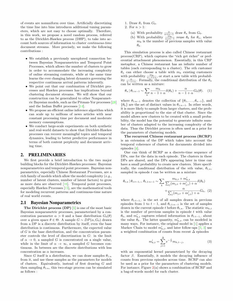
1. Draw θ1 from G0.2. For n > 1:
(a) With probability αα+n−1
draw θn from G0.
(b) With probability mkα+n−1
reuse θk for θn, wheremk is the number of previous samples with valueθk.
This simulation process is also called Chinese restaurantprocess(CRP), which captures the “rich get richer” or pref-erential attachment phenomenon. Essentially, in this CRPmetaphor, a Chinese restaurant has an infinite number oftables (each corresponding to a cluster). The nth customerθn can either choose a table with mk existing customerswith probability mk
n−1+α, or start a new table with probabil-
ity αn−1+α
. Formally, the conditional distribution of the θncan be written as a mixture:
θn | θ1:n−1 ∼∑k
mk
n− 1 + αδ(θk) +
α
n− 1 + αG0(θ). (1)
where θ1:n−1 denotes the collection of {θ1, . . . , θn−1}, and{θk} are the set of distinct values in θ1:n−1. In other words,it is more likely to sample from larger clusters, and the prob-ability is proportional to the size of that cluster. Since themodel allows new clusters to be created with a small proba-bility, the model has the potential to generate infinite num-ber of clusters adapted to the increasing complexity of thedata. Thus the Dirichlet process is often used as a prior forthe parameters of clustering models.
The recurrent Chinese restaurant process (RCRP)is an extension of the DP which takes into account thetemporal coherence of clusters for documents divided intoepisodes [4].
One can think of RCRP as a discrete-time sequence ofDPs, one for the data in each episode. The clusters in theseDPs are shared, and the DPs appearing later in time canhave a small probability to create new clusters. More specif-ically, the conditional distribution of the nth value, θt,n,sampled in episode t can be written as a mixture
θt,n | θ1:t−1,:, θt,1:n−1 ∼∑k
mk,t +m′k,t∑j(mj,t +m′j,t) + α
δ(θk)
+α∑
j(mj,t +m′j,t) + αG0, (2)
where θ1:t−1,: is the set of all samples drawn in previousepisodes from 1 to t − 1, and θt,1:n−1 is the set of samplesdrawn in the current episode t before θt,n. The statistic mk,t
is the number of previous samples in episode t with valueθk, and m′k,t captures related information in θ1:t−1,: aboutthe value θk. The latter quantity, m′k,t, can be modeled inmany ways. For instance, the original model in [4] applies aMarkov Chain to model m′k,t, and later follow-ups [2, 3] usea weighted combination of counts from recent ∆ episodes
m′k,t =
∆∑j=1
e− jβmk,t−j , (3)
with an exponential kernel parametrized by the decayingfactor β. Essentially, it models the decaying influence ofcounts from previous episodes across time. RCRP can alsobe used as a prior for the parameters of clustering models.For instance, Figure 2(a) shows a combination of RCRP anda bag-of-words model for each cluster.

However, RCRP requires artificially discretizing the timeline into episodes, which is unnatural for continuous-timeonline document streams. Second, different type of clus-ters is likely to occupy very different time scales, and it isnot clear how to choose the time window for each episodea-priori. Third, the temporal dependence of clusters acrossepisodes is hard-coded in Equation (3), and it is the same fordifferent clusters. Such design cannot capture the distinc-tive temporal dynamics of different type of clusters, such asrelated articles about disasters vs. Hollywood blockbusters,and fail to learn such dynamics from real data. We will usethe Hawkes process introduced next to address these draw-backs of RCRP when handling temporal dynamics.
2.2 Hawkes ProcessA temporal point process is a random process whose rea-
lization consists of a list of discrete events localized in time,{ti} with ti ∈ R+ and i ∈ Z+. Many different types of dataproduced in online social networks can be represented astemporal point processes, such as the event time of retweetsand link creations. A temporal point process can be equiva-lently represented as a counting process, N(t), which recordsthe number of events before time t. Let the history T bethe list of event time {t1, t2, . . . , tn} up to but not includingtime t. Then in a small time window dt between [0, t), thenumber of observed event is
dN(t) =∑ti∈T
δ(t− ti) dt, (4)
and hence N(t) =∫ t
0dN(s), where δ(t) is a Dirac delta
function. It is often assumed that only one event can happenin a small window of size dt, and hence dN(t) ∈ {0, 1}.
An important way to characterize temporal point pro-cesses is via the conditional intensity function — the stochas-tic model for the next event time given all previous events.Within a small window [t, t + dt), λ(t)dt is the probabilityfor the occurrence of a new event given the history T :
λ(t)dt = P {event in [t, t+ dt)|T } . (5)
The functional form of the intensity λ(t) is often designedto capture the phenomena of interests [1]. For instance,in a homogeneous Poisson process, the intensity is as-sumed to be independent of the history T and constant overtime, i.e., λ(t) = λ0 > 0. In an inhomogeneous Pois-son process, the intensity is also assumed to be indepen-dent of the history T but it can be a function varying overtime, i.e., λ(t) = g(t) > 0. In both case, we will use notationPoisson(λ(t)) to denote a Poisson process.
A Hawkes process captures the mutual excitation phe-nomena between events, and its intensity is defined as
λ(t) = γ0 + α∑ti∈T
γ(t, ti), (6)
where γ(t, ti) > 0 is the triggering kernel capturing temporaldependencies , γ0 > 0 is a baseline intensity independent ofthe history and the summation of kernel terms is history de-pendent and a stochastic process by itself. The kernel func-tion can be chosen in advance, e.g., γ(t, ti) = exp(− |t− ti|)or γ(t, ti) = I[t > ti], or directly learned from data.
A distinctive feature of a Hawkes process is that the oc-currence of each historical event increases the intensity bya certain amount. Since the intensity function depends onthe history T up to time t, the Hawkes process is essentially
a conditional Poisson process (or doubly stochastic Poissonprocess [17]) in the sense that conditioned on the history T ,the Hawkes process is a Poisson process formed by the su-perposition of a background homogeneous Poisson processwith the intensity γ0 and a set of inhomogeneous Poissonprocesses with the intensity γ(t, ti). However, because theevents in a past interval can affect the occurrence of theevents in later intervals, the Hawkes process in general ismore expressive than a Poisson process. Hawkes process isparticularly good for modeling repeated activities, such associal interactions [23], search behaviors [19], or infectiousdiseases that do not convey immunity.
Given a time t′ > t, we can also characterize the con-ditional probability that no event happens during [t, t′) andthe conditional density that an event occurs at time t′, usingthe intensity λ(t) [1], as
S(t′) = exp
(−∫ t′
t
λ(τ) dτ
), and f(t′) = λ(t′)S(t′). (7)
With these two quantities, we can express the likelihood ofa list of event times T = {t1, t2, . . . , tn} in an observationwindow [0, T ) with T > tn as
L =∏ti∈T
λ(ti) · exp
(∫ T
0
λ(τ) dτ
), (8)
which will be useful for learning the parameters of our modelfrom observed data. With the above backgrounds, now weproceed to describe our Dirichlet-Hawkes process.
3. DIRICHLET-HAWKES PROCESSThe key idea of Dirichlet-Hawkes process (DHP) is to
have the Hawkes Process model the rate intensity of events(e.g., the arrivals of documents), while the Dirichlet Pro-cess captures the diversity of event types (e.g., clusters ofdocuments). More specifically, DHP is parametrized by anintensity parameter λ0 > 0, a base distribution G0(θ) overa given space θ ∈ Θ and a collection of triggering kernelfunctions {γθ(t, t′)} associated with each event type of pa-rameter θ. Then, we can generate a sequence of samples{(ti, θi)} as follows :
1. Draw t1 from Poisson(λ0) and θ1 from G0(θ).2. For n > 1:
(a) Draw tn > tn−1 from Poisson(λ0 +
∑n−1i=1 γθi(t, ti)
).
(b) Draw θn from G0(θ) with probability :
λ0
λ0 +∑n−1i=1 γθi(tn, ti)
.
(c) Reuse θk for θn with probability :
λθk (tn)
λ0 +∑n−1i=1 γθi(tn, ti)
,
where λθk (tn) :=∑n−1i=1 γθi(tn, ti)I[θi = θk] is the
intensity of a Hawkes process for previous eventswith value θk.
Figure 1 gives an intuitive illustration of the Dirichlet-Hawkes Process. Compared to the Dirichlet process, theintensity parameter λ0 here serves the similar role to theconcentration parameter α in the Dirichlet process. Insteadof counting the number, mk, of samples within a cluster, the

t1 t4 Poisson(λ0)
Hawkes process for θ1t6 t7 t8
Hawkes process for θ2t2 t3 t5 t9
Figure 1: A sample from Dirichlet-Hawkes process. A
background Poisson process with intensity λ0 sampled
the starting time points t1 and t4 for two different event
types with the respective parameter θ1 and θ2. These
two initial events then generate Hawkes process of their
own, with events at time {t2, t3, t5, t9} and {t6, t7, t8}, re-
spectively.
Dirichlet-Hawkes process uses the intensity function λθk (t)of a Hawkes process which can be considered as a tempo-rally weighted count. For instance, if γθ(t, ti) = I[t > ti],then λθk (t) =
∑n−1i=1 I[t > ti]I[θi = θk] is equal to mk. If
γθ(t, ti) = exp(−|t − ti|), then λθk (t) =∑n−1i=1 exp(−|t −
ti|)I[θi = θk], and each previous event in the same clus-ter contributes a temporally decaying increment. Othertriggering kernels associated with θi can also be used orlearned from data. Thus the Dirichlet-Hawkes process ismore general than the Dirichlet process and can generateboth preferential-attachment type of clustering and rich tem-poral dynamics.
From a temporal point process of view, the generationof the event timing in Dirichlet-Hawkes process can also beviewed as the superposition of a Poisson process λ0 and sev-eral Hawkes processes (conditional Poisson processes), onefor each distinctive value of θd and with intensity λθd(t).Thus the overall event intensity is the sum of the intensitiesfrom individual processes [18]
λ̄(t) = λ0 +
D∑d=1
λθd(t),
where D is the total number of distinctive values {θi} in theDHP up to time t.
Therefore, the Dirichlet-Hawkes process can capture thefollowing four desirable properties :
1. Preferential attachment: Draw θn according to λθk (tn).The larger the intensity for a Hawkes process, the morelikely the next events is from that cluster.
2. Adaptive number of clusters: Draw θn according toλ0. There is always some probability of generatingnew cluster with λ0.
3. Self-excitation: This is captured by the intensity of theHawkes process λθk (t) =
∑n−1i=1 γθi(tn, ti)I[θi = θk].
4. Temporal decays: This is captured by the trigger-ing kernel function γθ(t, ti) which is typically decayingover time.
Finally, given the sequence of events (or samples) T ={(ti, θi)}ni=1 from a Dirichlet-Hawkes process, the likelihoodof the event arrival times can be evaluated based on (8) as
L(T ) = exp
(−∫ T
0
λ̄(τ)dτ
) ∏(ti,θi)∈T
λθi(ti), (9)
Compared to the recurrent Chinese restaurant process(RCRP) appeared in [4], a distinctive feature of the Dirichlet-Hawkes process is that there is no need to discretize the time
and divide events into episodes. Furthermore, the tempo-ral dynamics is controlled by more general triggering kernelfunctions, and can be statistically learned from data.
4. GENERATING TEXT WITH DHPAs we have defined the Dirichlet-Hawkes process (DHP),
we will use it as a prior for modeling a continuous-time doc-ument streams. The goal is to discover clusters from thedocument stream based on both contents and temporal dy-namics. Essentially, the set of {θi} sampled from the DHPwill be used as the parameters for document content model,and each cluster will have a distinctive value of θd ∈ {θi}.Furthermore, we will allow different clusters to have differenttemporal dynamics, with the corresponding triggering ker-nel drawn from a mixture of K base kernels. We will firstpresent the overall generative process of the model beforegoing into details of these components in Figure 2(b).
1. Draw t1 from Poisson(λ0), θ1 from Dir(θ|θ0), and αθ1from Dir(α|α0).
2. For each word v in document 1: wv1 ∼ Multi(θ1)3. For n > 1:
(a) Draw tn > tn−1 from Poisson(λ0 +
∑n−1i=1 γθi(tn, ti)
),
where γθi(tn, ti) =
K∑l=1
αlθi · κ(τl, tn − ti)
(b) Draw θn from Dir(θ|θ0) with probability
λ0
λ0 +∑n−1i=1 γθi(tn, ti)
, (10)
and draw αθn from Dir(α|α0)(c) Reuse previous θk for θn with probability
λθk (tn)
λ0 +∑n−1i=1 γθi(tn, ti)
, (11)
where λθk (tn) =∑n−1i=1 γθi(tn, ti)I[θi = θk].
(d) For each word v in document n:
wvn ∼ Multi(θn)
Content model. Many document content models canbe used here. For simplicity of exposition, we have used asimple bag-of-word language model for each cluster in theabove generative process. In this case, the base distributionG(θ) in the DHP is now chosen as a Dirichlet distribution,Dir(θ|θ0), with parameter θ0. Then, wvn, the vth word inthe nth document is sampled according to a multinomialdistribution
wvn ∼ Multi(θsn). (12)
where sn is the cluster indicator variable for the nth doc-ument, and the parameter θsn is a sample drawn from theDHP process.
Triggering kernel. We allow different clusters to havedifferent temporal dynamics, by representing the triggeringkernel function of the Hawkes Process as a non-negativecombination of K base kernel functions,i.e.,
γθ(ti, tj) =
K∑l=1
αlθ · κ(τl, ti − tj), (13)

wvn
snsn−1 sn+1
θs
θ0
wvn
snsj
tj tn
αsα0
n− 1
θs
θ0
wv,in
sinsj
tj
n− 1
skn
tkn
m− 1
tin
αsα0
θs
θ0
m
(a) Recurrent Chinese Restaurant Process (b) Dirichlet-Hawkes Process (c) Dirichlet-Hawkes Process with Missing Time
Figure 2: Generative models for different processes.
where tj < ti,∑l α
lθ = 1, αlθ > 0, and τi is the typical
reference time points, e.g., 0.5, 1, 8, 12, 24 hours etc.To simplify notations, define ∆ij = ti−tj , αθ = (α1
θ, . . . , αKθ )>
and k(∆ij) = (κ(τ1,∆ij), . . . , κ(τK ,∆ij))>, so γθ(ti, tj) =
α>θ k(∆ij). Since each cluster has its own set of kernel pa-rameters αθ, we are able to track their different evolvingprocesses. Given T = {(tn, θn)}Nn=1, the intensity functionof the cluster with parameter θ is represented as
λθ(t) =∑ti<t
α>θ k(t− ti)I[θi = θ], (14)
and the likelihood L(T ) of observing the sequence T beforetime T based on Equation (9) is
exp
−∑θi=θ
α>θ gθ − Λ0
∏θi=θ
∑tj<ti,θj=θ
α>θ k(∆ij), (15)
where glθ =∑ti<T,θi=θ
∫ Ttiκ(τl, t− ti)dt and Λ0 =
∫ T0λ0dt.
This can be done efficiently for many kernels, such as theGaussian RBF kernel [12], Rayleigh kernel [1], etc. Here,we choose the Gaussian RBF kernel κ(τl,∆) = exp(−(∆ −τl)
2)/2σ2l )/√
2πσ2l , so the integral glθ has the analytic form:
∑ti<T,θi=θ
1
2
(erfc
(− τl√
2σ2l
)− erfc
(T − ti − τl√
2σ2l
))(16)
Inexact event timing. In practice, news articles areusually automatically collected and indexed by web crawlers.Sometimes, due to unexpected errors or the available mini-mum timing resolution, we can observe a few m documentsat the same time tn. In this case, we assume that each ofthe m documents actually arrived between tn−1 and tn. Tomodel this rare situation, we can randomly pick tn and re-place the exact timestamps within the interval [tn, tn+m−1]by tn+m−1. See Figure 2(c) for the model modification totake that into account.
5. INFERENCEGiven a stream of documents {(di, ti)}ni=1, at a high level,
the inference algorithm alternates between two subroutines.The first subroutine samples the latent cluster membership(and perhaps the missing time) for the current documentdn by Sequential Monte Carlo [10, 11]; and then, the sec-ond subroutine updates the learned triggering kernels of therespective cluster on the fly.
Sampling the cluster label. Let s1:n and t1:n be the la-tent cluster indicator variables and document time for all thedocuments d1:n. For each sn, we have sn ∈ {0, 1, . . . , D},where D is the total number of distinctive values {θi}, andsn = 0 refers to the background Poisson process Poisson(λ0).In the streaming context, it is shown by [2, 3] that it wouldbe more suitable to efficiently draw a sample for the latentcluster labels s1:n shown in Figure 2(b) from P (s1:n|d1:n, t1:n)by reusing the past samples from P (s1:n−1|d1:n−1, t1:n), whichmotivates us to apply the Sequential Monte Carlo method [10,11, 2, 3]. Briefly, a particle keeps track of an approxima-tion of the posterior P (s1:n−1|d1:n−1, t1:n−1), where d1:n−1,t1:n−1, s1:n−1 represent all past documents, timestamps andcluster labels, and updates it to get an approximation forP (s1:n|d1:n, t1:n). We maintain a set of particles at the sametime, each of which represents a hypothesis about the latentrandom variables and has a weight to indicate how well itshypothesis can explain the data. The weight wfn of each par-ticle f ∈ {1, . . . , F} is defined as the ratio between the true
posterior and a proposal distribution wfn = P (s1:n|d1:n,t1:n)π(s1:n|d1:n,t1:n)
.
To minimize the variance of the resulting particle weight,we take π(sn|s1:n−1, d1:n, t1:n) to be the posterior distribu-tion P (sn|s1:n−1, d1:n, t1:n) [11, 2]. Then, the unnormalizedweight wfn can be updated by
wfn ∝ wfn−1 · P (dn|sfn, d1:n−1). (17)
Because the posterior is decomposed as P (sn|dn, tn, rest) ∼P (dn|sn, rest) · P (sn|tn, rest), by the Dirichlet-Multinomialconjugate relation, the likelihood P (dn|sn, rest) is given by
Γ(Csn\dn + V θ0
)∏Vv Γ
(Csn\dnv + Cdnv + θ0
)Γ (Csn\dn + Cdn + V θ0)
∏Kk Γ
(Csn\dnv + θ0
) , (18)
where Csn\dn is the word count of cluster sn excludingthe document dn, Cdn is the word count of document dn,
Csn,\dnv and Cdnv refer to the count of the vth word, and
V is the vocabulary size. Finally, P (sn|tn, rest) is the priorgiven by the Dirichlet-Hawkes process (10) and (11) as
P (sn = k|tn, rest) =
λθk
(tn)
λ0+∑n−1i=1 γθi
(tn,ti)if k occupied
λ0
λ0+∑n−1i=1 γθi
(tn,ti)otherwise
(19)
Updating the triggering kernel. Given sn, we denotethe respective triggering kernel αθsn by αsn for brevity. Bythe Bayesian rule, the posterior is given by P (αsn |Tsn) ∼
P (Tsn |αsn)P (αsn |α0), where Tsn = {(ti, si)|si = sn} is theset of events in cluster sn. We can either update the esti-mation of αsn by MAP for that the log-likelihood of (15)is concave in αsn . Alternatively, we can draw a set of sam-
ples{αisn
}Ni=1
from the prior P (αsn |α0) and calculate theweighted average:
α̂sn =
N∑i=1
wi ·αisn , (20)
where wi = P (Tsn |αisn)P (αisn |α0)/∑i P (Tsn |αisn)P (αisn |α0).
For simplicity, we choose the latter method in our implemen-tation.
Sampling the missing time. In the rare case whenm documents arrive with the same timestamp tn, the pre-cise document time is missing during the interval [tn−1, tn]shown in Figure 2(c). As a result, we need joint samplesfor
{(sin, t
in)}mi=1
where sin and tin are the cluster member-
ship and the precise arriving time for the ith document din.However, since m is expected to be small in practice, we canuse Gibbs sampling to draw samples from the distributionP (t1:m
n , s1:mn |t1:n−1, s1:n−1, rest) where s1:m
n and t1:mn are the
cluster labels and document time for the m documents inthe current nth interval. The initial values for t1:m
n can beassigned uniformly from the interval [tn−1, tn]. After fix-ing the sampled s1:m
n and the other{tkn}k 6=i, we are going
to draw a new sample tin′
from P (tin|sin, rest). Let Tsin\tin
be the set of all the document time excluding tin in clustersin. The posterior of tin is proportional to the joint likeli-hood P (tin|sin, Tsin\t
in, rest) ∝ P (tin, Tsin\t
in|sin, rest). There-
fore, we can apply Metropolis algorithm in one dimension todraw the next sample tin
′. Specifically, let’s first uniformly
draw tin′
from [tn−1, tn] and calculate the following ratio be-
tween the two joint likelihoods r =P (tin
′,Tsin\tin|s
in,rest)
P (tin,Tsin\tin|sin,rest)
. We
then accept tin′
if r > 1; otherwise, we accept it with theprobability r. With the new sample tin
′, we can update the
kernel parameter by (20). Finally, we need to update theparticle weight by considering the likelihood of generatingsuch m documents as
wfn ∝ wfn−1 ×m∏i=1
P (din|sf,in , d1:n−1, d1:m\in , rest)
×∏
s∈{sin}mi=1
P (ms|Ts, rest), (21)
where d1:m\in is the set of m documents excluding din, ms is
the number of documents with cluster membership s amongthe m documents, and Ts is the set of document time incluster s. Conditioned on the history up to tn, the Hawkesprocess is a Poisson process, and thus P (ms|Ts, rest) is sim-
ply a Poisson distribution with mean Λs =∫ tntn−1
λs(t)dt.
For Gaussian kernels, we can use (16) to obtain the analyticform of Λs. The overall pseudocode for Sequential MonteCarlo is formally presented in Algorithm 1, and the Gibbssampling framework is given by Algorithm 2.
Efficient Implementation. In order to scale with largedatasets, the online inference algorithm should be able toprocess each individual document in an expected constanttime. Particularly, the expected time cost of sampling thecluster label and updating the triggering kernel should not
Algorithm 1: The SMC Framework
1 Initialize wf1 to 1F
for all f ∈ {1 . . . F};2 for each event time tn, n = 1, 2, . . . do3 for f ∈ {1, . . . , F} do4 if one document dn at the time tn then5 sample sn from (19) and add tn;6 update the triggering kernel by (20);7 update the particle weight by (17);
8 else if m > 1 documents d1:mn with the same tn
then9 sample
{s1:mn
},{t1:mn
}by Algorithm 2;
10 update the particle weight by (21);
11 end
12 end13 Normalize particle weight;
14 if ‖wn‖−22 < threshold then
15 resample particles;
16 end
Algorithm 2: Gibbs sampling for cluster label and time
1 for iter = 1 to MaxIterG do2 if update cluster label sin then3 remove tin from cluster sin and update the
triggering kernel by (20);
4 draw a new sample sin′
from (19);
5 add tin into cluster sin′
and update the triggeringkernel by (20);
6 else if update document time tin then7 for iter = 1 to MaxIterM do
8 draw a new sample tin′ ∼ Unif(tn−1, tn);
9 if r =P (tin
′,Tsin\tin|s
in,rest)
P (tin,Tsin\tin|sin,rest)
> 1 then
tin ← tin′;
10 else tin ← tin′
with probability r;
11 end
12 update the triggering kernel of sin by (20);
13 end
14 end
grow with the amount of documents we have seen so far. Themost fundamental operation in Algorithm 1 and 2 is to eval-uate the joint likelihood (15) of all the past document timeto update the triggering kernel in every cluster. A straight-forward implementation requires repeated computation of asum of Gaussian kernels over the whole history, which tendsto be quadratic to the number of past documents.
Based on the fast decaying property that the Gaussiankernel decreases exponentially as the distance from its cen-ter increases quadratically, we can alleviate the problem byignoring those past time far away from the kernel center.Specifically, given an error tolerance ε, we only need to lookback until we reach the time
tu = tn −
(τm +
√−2σm log
(0.5ε
√(2πσ2
m)))
, (22)
where τm = maxl τl, σm = maxl σl and tn is the currentdocument time to guarantee that the error of the Gaussian
0
10
20
30
0 500 1000 1500 2000 2500time
intensity
Datacluster1cluster2
0.4
0.6
0.8
1.0
0.5 0.6 0.7 0.8 0.9overlap
NMI
Methods
DirichletHawkesRCRP
0
50
100
150
200
400 450 500 550time
intensity
Datacluster1cluster2
0.4
0.6
0.8
1.0
0.5 0.6 0.7 0.8 0.9overlap
NMI
Methods
DirichletHawkesRCRP
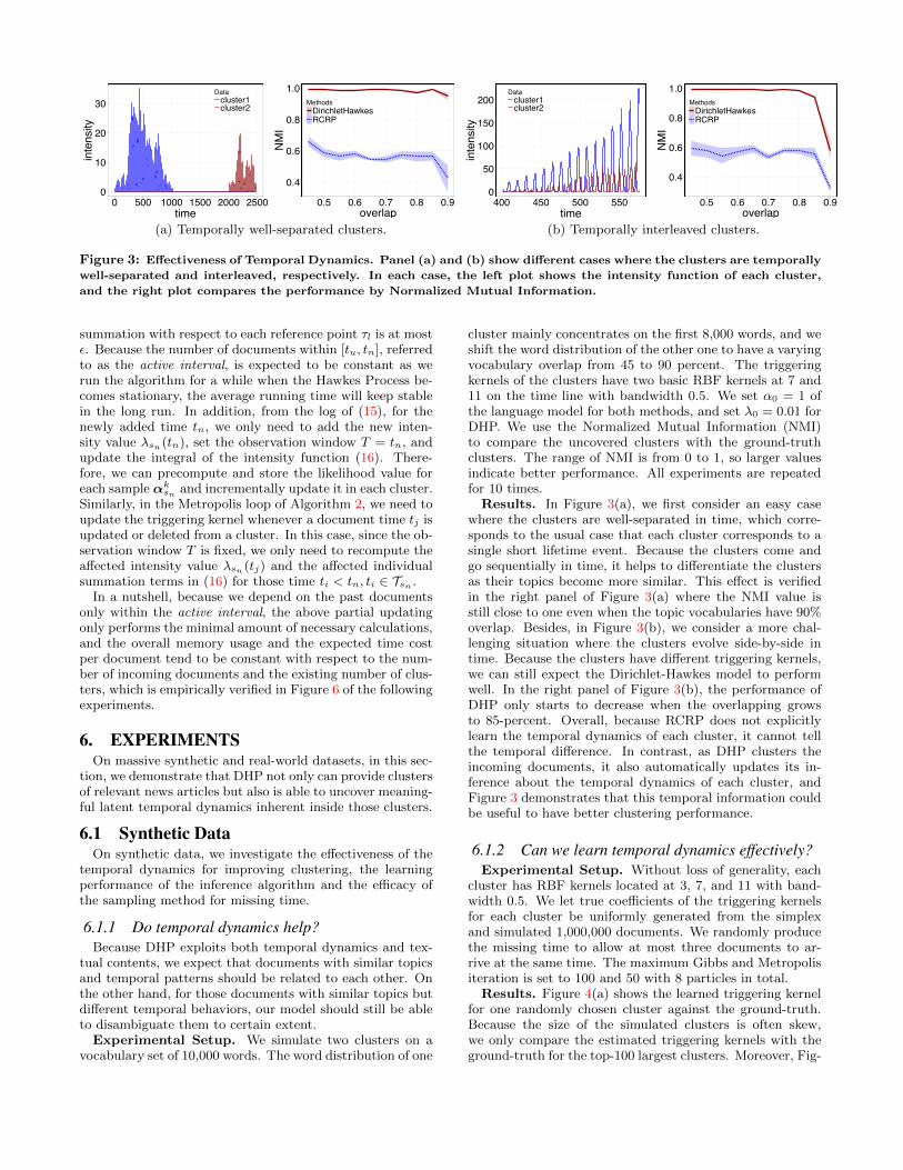
(a) Temporally well-separated clusters. (b) Temporally interleaved clusters.
Figure 3: Effectiveness of Temporal Dynamics. Panel (a) and (b) show different cases where the clusters are temporally
well-separated and interleaved, respectively. In each case, the left plot shows the intensity function of each cluster,
and the right plot compares the performance by Normalized Mutual Information.
summation with respect to each reference point τl is at mostε. Because the number of documents within [tu, tn], referredto as the active interval, is expected to be constant as werun the algorithm for a while when the Hawkes Process be-comes stationary, the average running time will keep stablein the long run. In addition, from the log of (15), for thenewly added time tn, we only need to add the new inten-sity value λsn(tn), set the observation window T = tn, andupdate the integral of the intensity function (16). There-fore, we can precompute and store the likelihood value foreach sample αksn and incrementally update it in each cluster.Similarly, in the Metropolis loop of Algorithm 2, we need toupdate the triggering kernel whenever a document time tj isupdated or deleted from a cluster. In this case, since the ob-servation window T is fixed, we only need to recompute theaffected intensity value λsn(tj) and the affected individualsummation terms in (16) for those time ti < tn, ti ∈ Tsn .
In a nutshell, because we depend on the past documentsonly within the active interval, the above partial updatingonly performs the minimal amount of necessary calculations,and the overall memory usage and the expected time costper document tend to be constant with respect to the num-ber of incoming documents and the existing number of clus-ters, which is empirically verified in Figure 6 of the followingexperiments.
6. EXPERIMENTSOn massive synthetic and real-world datasets, in this sec-
tion, we demonstrate that DHP not only can provide clustersof relevant news articles but also is able to uncover meaning-ful latent temporal dynamics inherent inside those clusters.
6.1 Synthetic DataOn synthetic data, we investigate the effectiveness of the
temporal dynamics for improving clustering, the learningperformance of the inference algorithm and the efficacy ofthe sampling method for missing time.
6.1.1 Do temporal dynamics help?Because DHP exploits both temporal dynamics and tex-
tual contents, we expect that documents with similar topicsand temporal patterns should be related to each other. Onthe other hand, for those documents with similar topics butdifferent temporal behaviors, our model should still be ableto disambiguate them to certain extent.
Experimental Setup. We simulate two clusters on avocabulary set of 10,000 words. The word distribution of one
cluster mainly concentrates on the first 8,000 words, and weshift the word distribution of the other one to have a varyingvocabulary overlap from 45 to 90 percent. The triggeringkernels of the clusters have two basic RBF kernels at 7 and11 on the time line with bandwidth 0.5. We set α0 = 1 ofthe language model for both methods, and set λ0 = 0.01 forDHP. We use the Normalized Mutual Information (NMI)to compare the uncovered clusters with the ground-truthclusters. The range of NMI is from 0 to 1, so larger valuesindicate better performance. All experiments are repeatedfor 10 times.
Results. In Figure 3(a), we first consider an easy casewhere the clusters are well-separated in time, which corre-sponds to the usual case that each cluster corresponds to asingle short lifetime event. Because the clusters come andgo sequentially in time, it helps to differentiate the clustersas their topics become more similar. This effect is verifiedin the right panel of Figure 3(a) where the NMI value isstill close to one even when the topic vocabularies have 90%overlap. Besides, in Figure 3(b), we consider a more chal-lenging situation where the clusters evolve side-by-side intime. Because the clusters have different triggering kernels,we can still expect the Dirichlet-Hawkes model to performwell. In the right panel of Figure 3(b), the performance ofDHP only starts to decrease when the overlapping growsto 85-percent. Overall, because RCRP does not explicitlylearn the temporal dynamics of each cluster, it cannot tellthe temporal difference. In contrast, as DHP clusters theincoming documents, it also automatically updates its in-ference about the temporal dynamics of each cluster, andFigure 3 demonstrates that this temporal information couldbe useful to have better clustering performance.
6.1.2 Can we learn temporal dynamics effectively?Experimental Setup. Without loss of generality, each
cluster has RBF kernels located at 3, 7, and 11 with band-width 0.5. We let true coefficients of the triggering kernelsfor each cluster be uniformly generated from the simplexand simulated 1,000,000 documents. We randomly producethe missing time to allow at most three documents to ar-rive at the same time. The maximum Gibbs and Metropolisiteration is set to 100 and 50 with 8 particles in total.
Results. Figure 4(a) shows the learned triggering kernelfor one randomly chosen cluster against the ground-truth.Because the size of the simulated clusters is often skew,we only compare the estimated triggering kernels with theground-truth for the top-100 largest clusters. Moreover, Fig-

0.0
0.1
0.2
0.3
0.4
0 5 10 15time
intensity
Methods
TrueLearned
0.05
0.10
0.15
0.20
0 1000 2000 3000 4000samples
MAE
0.048
0.051
0.054
0.057
21 22 23 24 25 26
particles
MAE
0.0
2.5
5.0
7.5
10.0
0.0 2.5 5.0 7.5 10.0theoretical
sample
(a) Triggering Kernel (b) MAE vs. # Samples (c) MAE vs. # Particles (d) QQ-Plot of Samples
Figure 4: (a) Learned triggering kernels of one cluster from 1,000,000 synthetic documents; (b) Mean absolute error
decreases as more samples are used for learning the triggering kernels; (c) A few particles are sufficient to have good
estimation; (d) Quantile plot of the intensity integrals from the sampled document time.
ure 4(b) presents the estimation error with respect to thenumber of samples drawn from the Dirichlet prior. As moresamples are used, the estimation performance improves, andFigure 4(c) shows that only a few particles are enough tohave good estimations.
6.1.3 How well can we sample the missing time?Finally, we check whether the sampled missing time from
Algorithm 2 are valid samples from a Hawkes Process.Experimental Setup. Fixing an observation window
T = 100, we first simulate a sequence of events HT with thetrue triggering kernels described in 6.1.2. Given HT , theform of the intensity function λ(t|HT ) is fixed. Next, weequally divide the interval [0, T ] into five partitions {Ti}5i=1,in each of which we incrementally draw ΛTi =
∫Tiλ(t|HT )dt
samples by Algorithm 2 using the true kernels. Then, wecollect the samples from all partitions to see whether thisnew sequence is a valid sample from the Hawkes Processwith the intensity λ(t|HT ).
Results. By the Time Changing Theorem [8], the in-
tensity integrals∫ titi−1
λ(τ)dτ from the sampled sequence
should conform to the unit-rate exponential distribution.Figure 4(d) presents the quantiles of the intensity integralsagainst the quantiles of the unit-rate exponential distribu-tion. It clearly shows that the points approximately lie onthe line indicating that the two distributions are very sim-ilar to each other and thus verifies that Algorithm 2 caneffectively generate samples for the missing time from theHawkes Process of each cluster.
6.2 Real World DataWe further examine our model on a set of 1,000,000 main-
stream news articles extracted from the Spinn3r2 datasetfrom 01/01 to 02/15 in 2011.
Experimental Setup. We apply the Named Entity Rec-ognizer from Stanford NER system [13] and remove commonstop-words and tokens which are neither verbs, nouns, noradjectives. The vocabulary of both words and named enti-ties is pruned to a total of 100,000 terms. We formulate thetriggering kernel of each cluster by placing a RBF kernel ateach typical time point : 0.5, 1, 8, 12, 24, 48, 72, 96, 120,144 and 168 hours with the respective bandwidth being setto 1, 1, 8, 12, 12, 24, 24, 24, 24, 24, and 24 hours, in or-der to capture both the short-term and long-term excitationpatterns. To enforce the sparse structure over the triggering
2http://www.icwsm.org/data/
kernels, we draw 4,096 samples from the Dirichlet prior withthe concentration parameter α = 0.1 for each cluster. Theintensity rate for the background Poisson process is set toλ0 = 0.1, and the Dirichlet prior of the language model isset to φ0 = 0.01. We report the results by using 8 particles.
Content Analysis. Figure 5 shows four discovered ex-ample stories, including the ‘Tucson shooting’ event3, themovie ‘Dark Knight Rises4’, Space Shuttle Endeavor’s lastmission5, and ‘Queensland Flooding’ disaster6. The top rowlists the top-100 frequent words in each story, showing thatDHP can deduce the clusters with meaningful topics.
Triggering Kernels. The middle row of Figure 5 givesthe learned triggering kernel of each story, which quantifiesthe influence over future events from the occurrence of thecurrent event. For the ‘Tucson Shooting’ story, its triggeringkernel reaches the peak within half an hour since its birth,decays quickly until the 30th hour, and then has a weaktailing influence around the 72nd hour, showing that it hasa strong short-term effect, that is, most related articles andposts arrive closely in time. In contrast, the triggering kernelof the story ‘Dark Knight Rises’ keeps stable for around 20hours before it decays below 10−4 by the end of a week. Thecontinuous activities of this period indicate that the currentevent tends to have influence over the events 20 hours later.
Temporal Dynamics. The bottom row of Figure 5 plotsthe respective intensity functions which indicate the popu-larity of the stories along time. We can observe that most re-ports of ‘Tucson Shooting’ concentrate within the followingtwo weeks starting from 01/13/2011 and fade out quickly bythe end of the month. In contrast, we can verify the longertemporal effect of the ‘Dark Knight Rises’ movie in Fig-ure 5(b) where the temporal gaps between two large spikesare about several multiples of the 20-hour period. Becausethis story is more about entertainment, including the arti-cles about Anne Hathaway’s playing of the Cat-woman inthe film as well as other related movie stars, it maintainsa certain degree of hotness by attracting people’s attentionas more production details of the movie are revealed. Forthe NASA event we can see in the intensity function of Fig-ure 5(c) the elapsed time between two observed large spikesis around a multiple of 45-hour, which is also consistent with
3http://en.wikipedia.org/wiki/2011_Tucson_shooting4http://www.theguardian.com/film/filmblog/2011/jan/13/batman-dark-knight-rises5http://en.wikipedia.org/wiki/Space_Shuttle_Endeavour6http://en.wikipedia.org/wiki/Cyclone_Yasi

Conte
nt
Analy
sis
Giffordsshoot
Tucsonhospit
doctor
Ga
bri
elle
Giff
ord
s
shot
wound
Kellycongresswoman
Arizona
feder
recoveri
Loughner
Houston
husbandkill
rehabbrain
victim
tube
condit
care
rehabilit
judg
Mark Kelly
Mark Kelly
injuri
wife
eye saturday
breath
memori
medic
progress
Fuller
astronaut
store
patient
bullet
speak
center
attack
side
gunman
Ariz.
Jared Loughner
Jared Loughner
critic
death
suspect
deadmental
chief
attempt
gu
n remov
interview
die
assassin
intens
therapi
aid
recov
watch
space
speech
improv
rampag
fire
University Medical Center
hear
polit
facil
arriv
constitu
leg
accus
physic
ho
ld
su
nd
ay
injur
groceri
ha
nd
health
court
walk
statementarm
gunshotPhoenix
girl
murder
de
cis
respond
abil
sheriff
investig
su
pe
rma
rke
tstaff
min
ut
filmmovi
da
rk
star
knightrise
role
cast
superman
trailer
actor
exclus
director
fea
tur
confirmtv
seri
charact
produc
super
ca
two
ma
n
batman
captain
Anne Hathaway
sp
ot
award
poster
bowl
project
oscar
ba
ne
aveng
dvd
Tom Hardy
screen
mo
vie
we
b
love wh
ite
steel
hu
lk
sn
ow
win
ne
r
script
book
contestshoot
latest
twilight
rem
ak
su
nd
an
c
reveal
actress
franchis
transform
watch
Kri
ste
n S
tew
art
Lois Lane
dead
sequel
iron
fan
va
mp
ir
rediblnomin
america
upcom
comic
singer
horror
xlv
hollywood
origin
ad
ap
t
avatar
clip
bring
James Bond
superhero
imag
chat
Jo
se
ph
Go
rdo
n-L
evitt
pictur
scene
joker
british
reb
oo
t
prize
list
riddler
woman
choic
alien
web
titl
eye
detail
art
wo
rk
break
academi
ve
rsio
n
spacelaunch
NASA
shuttl
endeavour
mission
flight
rocket
vehicl
crew
cost
orbit
program
station
engin
astronaut
challeng stage
quot
design
replisatellit
test
payload
fli
commerci
locat
land
spacecraft
build
capabl
agenc
mar
hlvcargo
technologtank
fuel
propel
modul
billion
dragon
command
booster
carri
budget
fund
center
thread
schedul
heavi
dock
pad
experi
control
mass
complet
Kelly
target
perform
explor
discoveri
project
futur
train
ton
capsul
Congress
idea
lift
afford
transfer
rate
offlin
human
contract
studi
onlin
assumatlas
apollo
russian
US
pressur small
exist
april
suppli
facil
goal
expens
falcon
ISS
iss
EELV
moon
propos
agre
replac
process cyclo
n
storm
Queensland
windcoast Australia
damagYasi
evacuflood
no
rth
resid
Cairnstown
warn
categori
raintropic
centrsu
rg
devast
Townsvilleworst
Bligh
communiti prepar
waterroof
Inn
isfa
il
yasi
premier
region
south
emerg
sh
elte
r
morn
de
str
uct
gustdanger
forecast
Anna Bligh
inland
thousand
Cardwell
sidebar
weather
tre
e
milems
disast
Cyclo
ne
Ya
si
Larry
monster
tourist
kill
build
Tullypath
coastal
co
ve
rag
coal
Bureau of Meteorology
generat
Mission Beach
heavinortheast
mph
window
tide
crop
mine
kilometr
mayorstreet
eye
landfal
center
sugar
cut
minist
sce
ne
terrifi
bureau
batternorthern
death
reach
kph
flig
ht
mid
nig
ht
sta
y
threat
de
str
oy
flee
impact
hospit
bear Brisbane
bring
safe
Tri
gger
ing
Ker
nel
3 days
Triggering Kernel
10-3.0
10-2.5
10-2.0
10-1.5
10-1.0
10-0.5
100.0 100.5 101.0 101.5102.0
time
inte
nsity
20 hours
10-4
10-3
10-2
10-1
100.0 100.5 101.0 101.5102.0
time
2 days
45 hours
10-4
10-3
10-2
10-1
100.0 100.5 101.0 101.5102.0
time
1.5 hours
24 hours7 days
10-5
10-4
10-3
10-2
10-1
100.0 100.5 101.0 101.5102.0
time
Tem
pora
lD
ynam
ics
Intensity Function
0
10
20
30
1/13 1/18 1/23 1/28 2/3time
inte
nsity
120 hours
100 hours
0
5
10
1/18 1/23 1/28 2/3 2/8time
95 hours
0
5
10
1/13 1/18 1/23 1/28 2/3 2/8time
24 hours
0
10
20
30
1/28/11 2/3/11 2/8/11time
(a) Tucson Shooting (b) Dark Knight Rise (c) Endeavour (d) Queensland Flooding
Figure 5: Four example stories extracted by our model, including the ‘Tucson Shooting’ event, the movie of ‘Dark
Knight Rises’, Space Shuttle’s final mission and Queensland flooding disaster. For each story, we list the top 100 most
frequent words on the top row. The middle row shows the learned triggering kernel in the log-log scale, and the last
row presents the respective intensity functions along time.
its corresponding triggering kernel. Finally, for the eventof ‘Queensland Flooding’, the ‘Cyclone Yasi’ intensified toa Category 3 cyclone on 01/31/2011, to a Category 4 on02/01/2011, and to a Category 5 on 02/02/20117. Thesecritical events again coincide with the observed spikes inthe intensity function of the story in Figure 5(d). Becausethe intensity functions depend on both the triggering ker-nels and the arriving rate of news articles, news reports ofemergent incidents and disasters tend to be concentrated intime to form strong short-term clusters with higher magni-tude of intensity values. In Figure 5, the intensity functionsof both ‘Tucson Shooting’ and ‘Queensland Flooding’ havevalue greater than 20. In contrast, other types of stories inentertainment and scientific explorations might have contin-uous longer-term activities as more and more related detailsget revealed. Overall, the ability of uncovering topic-specificclusters with learned latent temporal dynamics of our modelprovides a better and intuitive way to track the trend of eachevolving story in time.
Scalability. Figure 6(a) shows the scalability of our learn-ing algorithm. Since the number of clusters grows logarith-mically as the number of data points increases for CRP, weexpect the average time cost of processing each documentis keeping roughly constant after running for a long timeperiod. This is verified in Figure 6(a) where after the build-up period, the average processing time per 10,000-documentkeeps stable.
7http://en.wikipedia.org/wiki/Cyclone_Yasi
0.0
0.1
0.2
0.3
1 ×10+4 2.5 ×10+5 5 ×10+5 7.5 ×10+5 1 ×10+6
#docs
time(s)
10-6.0
10-5.5
10-5.0
10-4.5
104.0 104.5 105.0 105.5 106.0
#docs
MAE
MethodsHawkesDirichletRCRP
(a) Scalability (b) Time prediction
Figure 6: Scalability and time prediction in real world
news stream.
Prediction. Finally, we evaluate how well the learnedtemporal model of each cluster can be used for predictingthe arrival of the next event. Starting from the 5,000thdocument, we predict the possible arriving time of the nextdocument for the clusters with size larger than 100. SinceRCRP does not learn the temporal dynamics, we use theaverage inter-event gap between two successive documentsas the predicted time interval between the most recent doc-ument and the next one in the future. For DHP, we simulatethe next event time based on the learned triggering kernelsand the timestamps of the documents observed so far. Wetreat the average of five simulated time as our final pre-diction and report the cumulative mean absolute predictionerror in Figure 6(b) in the log-log scale. As more docu-
ments are observed, the prediction errors of both methodsdecrease. However, the prediction performance of DHP iseven better from the very beginning when the number ofdocuments is still relatively small, showing that the Hawkesmodel indeed can help to capture the underlying temporaldynamics of the evolution of each cluster.
7. DISCUSSIONSIn addition to RCRP, several other well-known processes
can also be incorporated into the framework of DHP. Forinstance, we may generalize the Pitman-Yor Process [21]to incorporate the temporal dynamics. This simply bringsback the constant rate for each Hawkes Process. A smalltechnical issue arises from the fact that if we were to decaythe counts mk,t as in the RCRP, we would obtain negativecounts frommk,t−a, where a is the parameter of the Pitman-Yor Process to increase the skewness of the cluster size dis-tribution. However, this can be addressed, e.g., by clippingthe terms by 0 via max(0,mk,t). In this form we obtain amodel that further encourages the generation of new topicsrelative to the RCRP. Moreover, The Distance-DependentChinese Restaurant Process (DD-CRP) of [6] attempts toaddress spatial interactions between events. This general-izes the CRP and, with a suitable choice of distance func-tion, can be shown to contain the RCRP as a special case.The same notion can be used to infer spatial / logical inter-actions between Hawkes Processes to obtain spatiotemporaleffects. That is, we simply use spatial excitation profiles tomodel the rate of each event.
To conclude, we present the Dirichlet-Hawkes Process whichis a scalable probabilistic generative model inheriting theadvantages from both the Bayesian nonparametrics and theHawkes Process to deal with asynchronous streaming datain an online manner. Experiments on both synthetic andreal world news data demonstrate that by explicitly mod-eling the textual content and the latent temporal dynamicsof each cluster, it provides an elegant way to uncover top-ically related documents and track their evolution in timesimultaneously.
References[1] O. Aalen, O. Borgan, and H. Gjessing. Survival and
event history analysis: a process point of view. Springer,2008.
[2] A. Ahmed, J. Eisenstein, Q. Ho, E. P. Xing, A. J.Smola, and C. H. Teo. The topic-cluster model. InArtificial Intelligence and Statistics AISTATS, 2011.
[3] A. Ahmed, Q. Ho, J. Eisenstein, E. Xing, A. Smola,and C. Teo. Unified analysis of streaming news. InProceedings of WWW, Hyderabad, India, 2011. IW3C2,Sheridan Printing.
[4] A. Ahmed and E. Xing. Dynamic non-parametric mix-ture models and the recurrent chinese restaurant pro-cess: with applications to evolutionary clustering. InSDM, pages 219–230. SIAM, 2008.
[5] C. Antoniak. Mixtures of Dirichlet processes with ap-plications to Bayesian nonparametric problems. Annalsof Statistics, 2:1152–1174, 1974.
[6] D. Blei and P. Frazier. Distance dependent chineserestaurant processes. In ICML, pages 87–94, 2010.
[7] D. M. Blei and J. D. Lafferty. Dynamic topic models.In ICML, pages 113–120, 2006.
[8] D. Daley and D. Vere-Jones. An introduction to thetheory of point processes: volume II: general theory andstructure, volume 2. Springer, 2007.
[9] Q. Diao and J. Jiang. Recurrent chinese restaurantprocess with a duration-based discount for event iden-tification from twitter. In SDM, 2014.
[10] A. Doucet, J. F. de Freitas, K. Murphy, and S. Rus-sell. Rao-blackwellised particle filtering for dynamicbayesian networks. In C. Boutilier and M. Goldszmidt,editors, UAI, pages 176–183, SF, CA, 2000.
[11] A. Doucet, N. de Freitas, and N. Gordon. Sequen-tial Monte Carlo Methods in Practice. Springer-Verlag,2001.
[12] N. Du, L. Song, A. Smola, and M. Yuan. Learningnetworks of heterogeneous influence. In NIPS, pages2789–2797, 2012.
[13] J. R. Finkel, T. Grenager, and C. Manning. Incorporat-ing non-local information into information extractionsystems by gibbs sampling. In ACL, 2005.
[14] T. Griffiths and Z. Ghahramani. The indian buffet pro-cess: An introduction and review. Journal of MachineLearning Research, 12:1185–1224, 2011.
[15] A. G. Hawkes. Spectra of some self-exciting and mutu-ally exciting point processes. Biometrika, 58(1):83–90,1971.
[16] N. L. Hjort, C. Holmes, P. Muller, and S. G. Walker.Bayesian Nonparametrics. Cambridge University Press,2010.
[17] J. Kingman. On doubly stochastic poisson processes.Mathematical Proceedings of the Cambridge Philosoph-ical Society, pages 923–930, 1964.
[18] J. F. C. Kingman. Poisson processes, volume 3. Oxforduniversity press, 1992.
[19] L. Li, H. Deng, A. Dong, Y. Chang, and H. Zha. Identi-fying and labeling search tasks via query-based hawkesprocesses. In KDD, pages 731–740, 2014.
[20] C. Suen, S. Huang, C. Eksombatchai, R. Sosic, andJ. Leskovec. Nifty: A system for large scale informationflow tracking and clustering. In WWW, 2013.
[21] Y. W. Teh. A hierarchical bayesian language modelbased on pitman-yor processes. In Proceedings of the21st International Conference on Computational Lin-guistics and the 44th annual meeting of the Associationfor Computational Linguistics, pages 985–992, 2006.
[22] X. Wang and A. McCallum. Topics over time: A non-markov continuous-time model of topical trends. InKDD, 2006.
[23] K. Zhou, H. Zha, and L. Song. Learning social infectiv-ity in sparse low-rank networks using multi-dimensionalhawkes processes. In AISTATS, 2013.