dirichlet process 4 - umd
TRANSCRIPT
Dirichlet Mixtures, the Dirichlet Process, and the
Topography of Amino Acid Multinomial Space
National Center for Biotechnology Information
National Library of Medicine
National Institutes of Health
Bethesda, Maryland
Stephen Altschul

Motivational Problem
How should one score the alignment of a single letter
to a column of letters from a multiple alignment?
V
F
V
L
M
Pairwise Alignment Scores
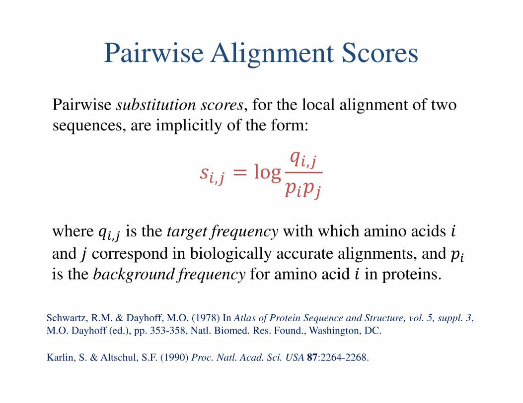
Pairwise substitution scores, for the local alignment of two
sequences, are implicitly of the form:
��,� = log �,���
where �,� is the target frequency with which amino acids �and � correspond in biologically accurate alignments, and �is the background frequency for amino acid � in proteins.
Schwartz, R.M. & Dayhoff, M.O. (1978) In Atlas of Protein Sequence and Structure, vol. 5, suppl. 3,
M.O. Dayhoff (ed.), pp. 353-358, Natl. Biomed. Res. Found., Washington, DC.
Karlin, S. & Altschul, S.F. (1990) Proc. Natl. Acad. Sci. USA 87:2264-2268.

Generalization to Multiple Alignments
The score for aligning an amino acid to a multiple alignment
column should be
�� = log ��where � is the estimated probability of observing amino acid �in that column.
Transformed motivational problem:
How should one estimate the twenty
components of from a multiple
alignment column that may contain
only a few observed amino acids?
V
F
V
L
A Bayesian Approach
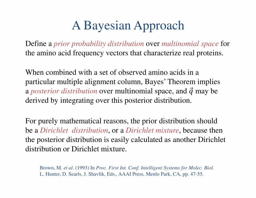
Define a prior probability distribution over multinomial space for
the amino acid frequency vectors that characterize real proteins.
When combined with a set of observed amino acids in a
particular multiple alignment column, Bayes’ Theorem implies
a posterior distribution over multinomial space, and may be
derived by integrating over this posterior distribution.
For purely mathematical reasons, the prior distribution should
be a Dirichlet distribution, or a Dirichlet mixture, because then
the posterior distribution is easily calculated as another Dirichlet
distribution or Dirichlet mixture.
Brown, M. et al. (1993) In Proc. First Int. Conf. Intelligent Systems for Molec. Biol.
L. Hunter, D. Searls, J. Shavlik, Eds., AAAI Press, Menlo Park, CA, pp. 47-55.

Multinomial Space
A multinomial on an alphabet of � letters is a vector of � positive
probabilities that sum to 1.
The multinomial space Ω� is the space of all multinomials on � letters.
Because of the constraint on the components of a multinomial,
Ω� is � − 1 dimensional.
Example: Ω� is a 2-dimensional
equilateral triangle.
(0,1,0)
(0,0,1)
(1,0,0)
For proteins, we will be interested
in the 19-dimensional multinomial
space ��.
The Dirichlet Distribution
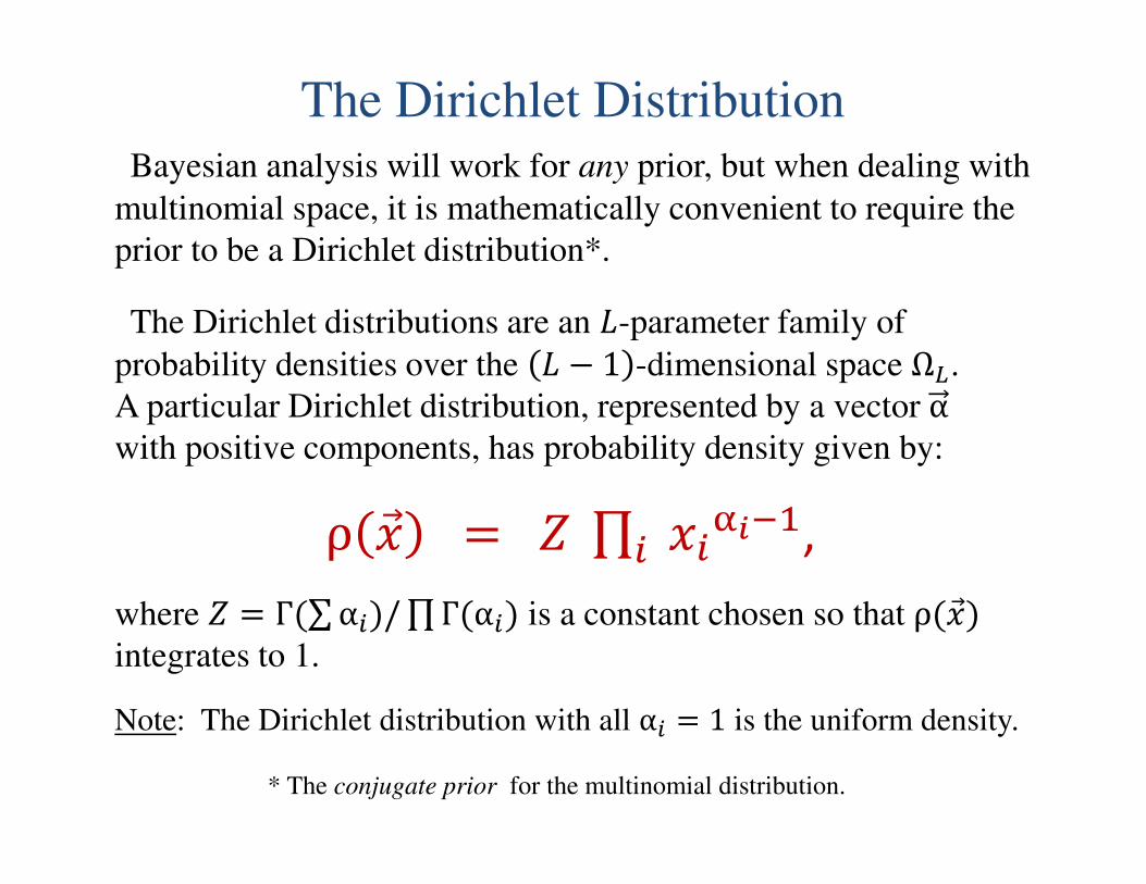
Bayesian analysis will work for any prior, but when dealing with
multinomial space, it is mathematically convenient to require the
prior to be a Dirichlet distribution*.
The Dirichlet distributions are an �-parameter family of
probability densities over the � − 1 -dimensional space Ω�.
A particular Dirichlet distribution, represented by a vector αwith positive components, has probability density given by:
ρ � = �∏ ������� ,
where � = Г(∑α�)/∏Г(α�) is a constant chosen so that ρ(� )integrates to 1.
* The conjugate prior for the multinomial distribution.
Note: The Dirichlet distribution with all α� = 1 is the uniform density.

How to Think About Dirichlet Distributions
.
Define the “concentration parameter” α
to be ∑α�. Then the center of mass of
the Dirichlet distribution is = α/α.
The greater α, the greater the concentration of probability near .
By Bayes’ theorem, the observation of a single letter “%”
transforms the Dirichlet prior α into a Dirichlet posterior α′with identical parameters, except that α′' = α' + 1.
A Dirichlet distribution may be alternatively parameterized by: (p, α).

Bayes at Work
0 0.2 0.4 0.6 0.8 10
1
2
3
0 0.2 0.4 0.6 0.8 10
1
2
3
0 0.2 0.4 0.6 0.8 10
1
2
3
0 0.2 0.4 0.6 0.8 10
1
2
3
0 0.2 0.4 0.6 0.8 10
1
2
3
0 0.2 0.4 0.6 0.8 10
1
2
3
0 0.2 0.4 0.6 0.8 10
1
2
3
0 0.2 0.4 0.6 0.8 10
1
2
3
0 0.2 0.4 0.6 0.8 10
1
2
3
Here, we begin with the
uniform Dirichlet prior
(1,1) for the probability of
“heads”, and observe its
transformation, after
successive observations
HTHHTHTH, into the
posteriors (2,1), (2,2),
(3,2), etc.
At any given stage, the
center of mass (i.e. the
expected probability of
heads) is given by:
# + ,�# + ,� ,[# . ,�]
Note: The 2-parameter Dirichlet distributions, which take the
form �����(1 − �)0��, are also called Beta distributions.
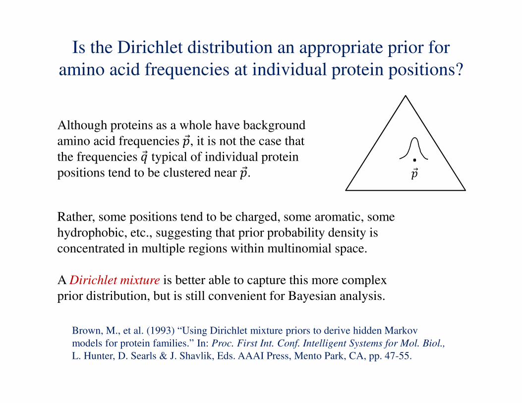
Is the Dirichlet distribution an appropriate prior for
amino acid frequencies at individual protein positions?
.
Although proteins as a whole have background
amino acid frequencies , it is not the case that
the frequencies typical of individual protein
positions tend to be clustered near .
Rather, some positions tend to be charged, some aromatic, some
hydrophobic, etc., suggesting that prior probability density is
concentrated in multiple regions within multinomial space.
A Dirichlet mixture is better able to capture this more complex
prior distribution, but is still convenient for Bayesian analysis.
Brown, M., et al. (1993) “Using Dirichlet mixture priors to derive hidden Markov
models for protein families.” In: Proc. First Int. Conf. Intelligent Systems for Mol. Biol.,
L. Hunter, D. Searls & J. Shavlik, Eds. AAAI Press, Mento Park, CA, pp. 47-55.

Dirichlet Mixtures
A Dirichlet mixture consists of 1 Dirichlet components, associated
respectively with positive “mixture parameters” 2�, 2�, … ,24 that
sum to 1. Only 1 − 1 of these parameters are independent.
Each Dirichlet component has the
usual � free “Dirichlet parameters”,
so an 1-component Dirichlet mixture
has a total of 1 � + 1 − 1 free
parameters.
The density of a Dirichlet mixture is
defined to be a linear combination of
those of its constituent components.
A Dirichlet mixture max be visualized as a
collection of probability hills in multinomial space.

Where do Dirichlet Mixture Priors Come From?
No one knows how to construct a Dirichet
mixture prior from first principles.
This is an instance of the classic, difficult problem of optimization in a rough,
high-dimensional space. The only practical approaches known are heuristic.
Given a large number of multiple alignment columns, we seek the
maximum-likelihood 1-component D.M., i.e. the one that best
explains the data.
A Dirichlet mixture prior should capture our knowledge about amino
acid frequencies within proteins. However:
So we invert the problem: Like substitution matrices, D.M. priors may
be derived from putatively accurate alignments of related sequences.
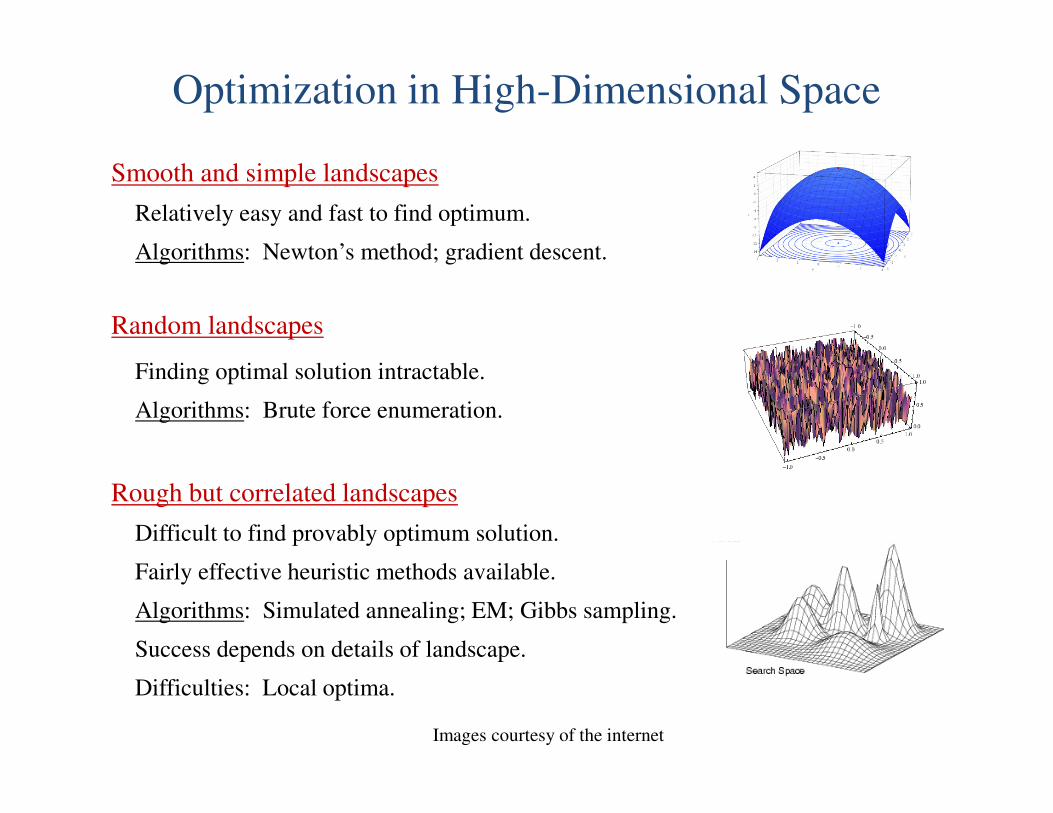
Optimization in High-Dimensional Space
Smooth and simple landscapes
Random landscapes
Rough but correlated landscapes
Relatively easy and fast to find optimum.
Algorithms: Newton’s method; gradient descent.
Difficult to find provably optimum solution.
Fairly effective heuristic methods available.
Algorithms: Simulated annealing; EM; Gibbs sampling.
Success depends on details of landscape.
Finding optimal solution intractable.
Algorithms: Brute force enumeration.
Difficulties: Local optima.
Images courtesy of the internet

Heuristic Algorithms
Ye, X., et al. (2011) "On the inference of Dirichlet mixture priors for protein sequence
comparison." J. Comput. Biol. 18:941-954.
Geman, S. & Geman, D. (1984) “Stochastic relaxation, Gibbs distributions, and the Bayesian
restoration of images.” IEEE Trans. Pattern Analysis and Machine Intelligence 6:721-741.
Metropolis, N., et al. (1953) “Equation of state calculations by fast computing machines.”
J. Chem. Phys. 21:1087-1092.
The Metropolis algorithm and simulated annealing
Gibbs sampling
applied to Dirichlet mixtures
Nguyen, V.-A., et al. (2013) “Dirichlet mixtures, the Dirichlet process, and the structure
of protein space." J. Comput. Biol. 20:1-18.
Dempster, A.P., et al. (1977) "Maximum likelihood from Incomplete data via the EM
algorithm." J. Royal Stat. Soc., Series B 39:1-38.
Expectation maximization (EM)
applied to Dirichlet mixtures
Brown, M., et al. (1993) In: Proc. First Int. Conf. Intelligent Systems for Molec.
Biol., L. Hunter, D. Searls, J. Shavlik, Eds., AAAI Press, Menlo Park, CA, pp. 47-55.

Gibbs Sampling for Dirichlet Mixtures
Find: The 1 Dirichlet components that maximize the
likelihood of the data
Given: 5 multiple alignment columns
Algorithm
1) Initialize by associating columns with components
2) Derive the parameters for each Dirichlet component
from the columns assigned to it
3) In turn, sample each column into a new component,
using probabilities proportional to column likelihoods
4) Iterate
How Many Dirichlet Components
Should There Be?
Problem: The more components, the greater the likelihood
of the data. The criterion of maximum-likelihood alone
leads to overfitting.
One solution: The Minimum Description Length (MDL)
principle.
Grunwald, P.D. (2007) The Minimum Description Length Principle. MIT Press, Cambridge, MA.
Idea: Maximize the likelihood of the data.

A model that is too simple underfits the data
From: “A tutorial introduction to the minimum description
length principle” by Peter Grünwald
A simple model, i.e. one
with few parameters, will
have low complexity but
will not fit the data well.
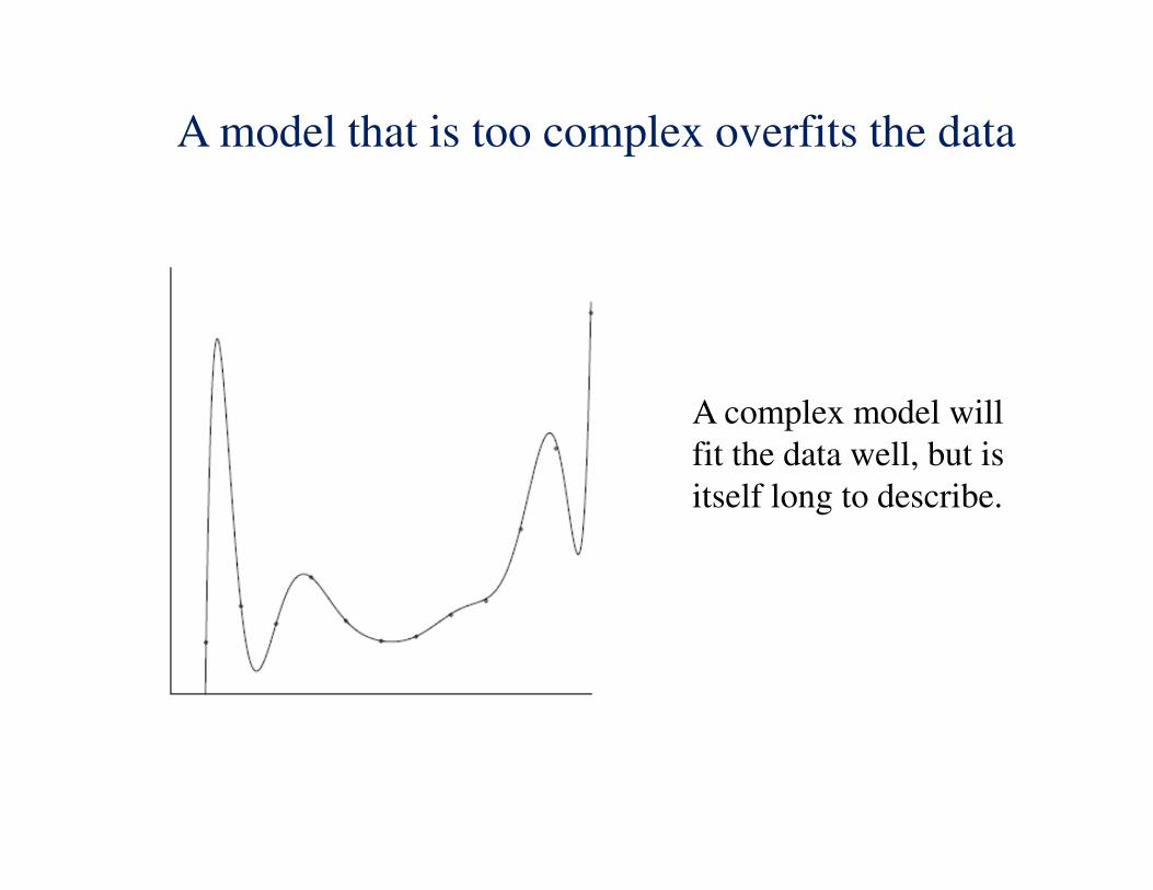
A model that is too complex overfits the data
A complex model will
fit the data well, but is
itself long to describe.

A model with an appropriate number of parameters
Everything should be made as
simple as possible, but not
simpler. – Albert Einstein
A model should be as detailed
as the data will support, but no
more so. – MDL principle

The Minimum Description Length Principle
A set of data 6 may be described by a parametrized theory,
chosen from a set of theories called a model, 7.
MDL theory defines the complexity of a model, COMP 7 .
It may be thought of as the log of the effective number of
independent theories the model contains.
DL 6 7 , the description length of 6 given 7, is the negative
log probability of 6 implied by the maximum-likelihood theory
contained in 7.
The MDL principle asserts that the best model for describing 6is that which minimizes: DL 6 7 + COMP 7 .
Grunwald, P.D. (2007) The Minimum Description Length Principle. MIT Press, Cambridge, MA.
Effect: More complex models are penalized
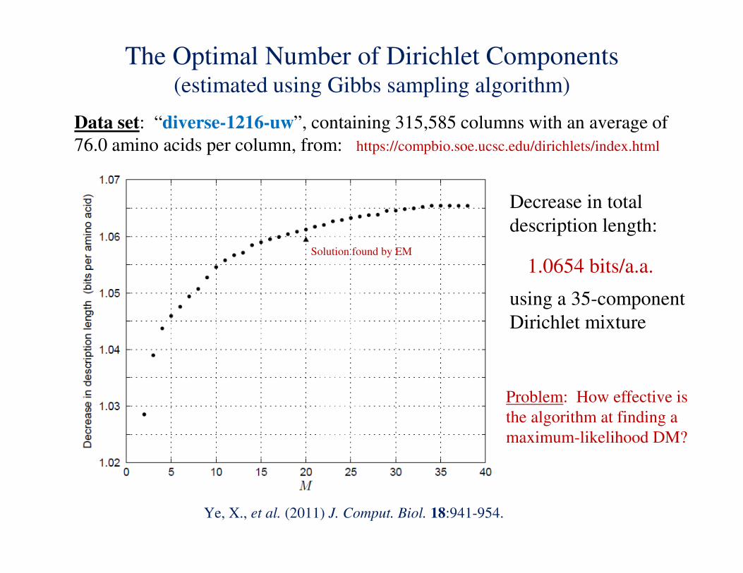
The Optimal Number of Dirichlet Components (estimated using Gibbs sampling algorithm)
Data set: “diverse-1216-uw”, containing 315,585 columns with an average of
76.0 amino acids per column, from: https://compbio.soe.ucsc.edu/dirichlets/index.html
Ye, X., et al. (2011) J. Comput. Biol. 18:941-954.
Decrease in total
description length:
1.0654 bits/a.a.
using a 35-component
Dirichlet mixture
Problem: How effective is
the algorithm at finding a
maximum-likelihood DM?
Solution found by EM

The Dirichlet Process
The Dirichlet Process (DP) is used to model mixtures with
an unknown or an unbounded number of components.
The name derives from a generalization of the Dirichlet
distribution to an infinite number of dimensions, to model
the weights of these components.
A DP may be thought of as assigning a generalized prior probability to mixtures with an
infinite of components.
A DP is completely specified by two elements:
A prior distribution @ over the parameters of the underlying distribution
Many distributions may be modeled as mixtures of an underlying
distribution. For example, the distribution of points along a line
may be modeled by a mixture of normal distributions.
A positive real hyperparameter, which we will call γ, which defines a prior
on the weights of the components
The smaller γ, the greater the implied concentration of weight in a few components.
Antoniak, C.E. (1974) Ann. Stat. 2:1152-1174.
(0,1,0)
(0,0,1)
(1,0,0)Component
weights

The Chinese Restaurant Process
A restaurant with an infinite number of tables.
People enter sequentially and sit randomly at tables, following these probabilities:
At an occupied table A, with probability proportional to the number of
people 5B already seated there;
At a new, unoccupied table, with probability proportional to γ.
Example: 8 people already seated: 3 at Table 1; 5 at Table 2; γ = 2.Probability to sit at Table 1: 0.3
Probability to sit at Table 2: 0.5
Probability to sit at a new table: 0.2
Each table corresponds to a component, with its parameters chosen randomly
according to the prior distribution @.
The proportion of people seated at a table corresponds to its weight.
Ferguson, T.S. (1973) Ann. Stat. 1:209-230.

When sampling a column E into a component:
If E was the only column associated with its old component, abolish
that component.
Allow E to seed a new component, with probability proportional to γ.
This may be calculated by integrating γProb E Prob( |α) over Ω��and Dirichlet parameter space, using the prior density @.
If a new component is created, sample its parameters, as below.
Dirichlet-Process Modifications
to the Gibbs Sampling Algorithm
When calculating Dirichlet parameters for a component:
Sample the parameters from the posterior distribution implied by @ and
the columns assigned to the component.
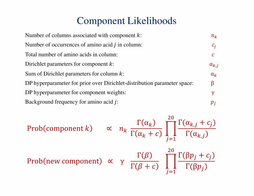
Component Likelihoods
Prob componentA ∝ NB Γ αB
Γ αB + P QΓ(αB,� + P�)Γ(αB,�)
��
�R�
Prob newcomponent ∝ γ Γ TΓ T + P QΓ(β� + P�)
Γ(β�)��
�R�
Total number of amino acids in column: PNumber of occurrences of amino acid � in column: P�
Dirichlet parameters for component A: αB,�Sum of Dirichlet parameters for column A: αBDP hyperparameter for prior over Dirichlet-distribution parameter space: βDP hyperparameter for component weights: γBackground frequency for amino acid �: �
Number of columns associated with component A: NB

Decrease in Total Description Length as a Function
of the Dirichlet Process Hyperparameters β and γ
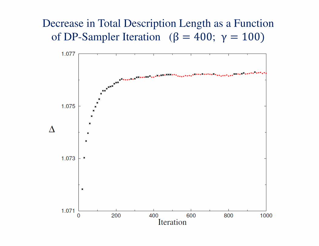
Decrease in Total Description Length as a Function
of DP-Sampler Iteration (β = 400; γ = 100)
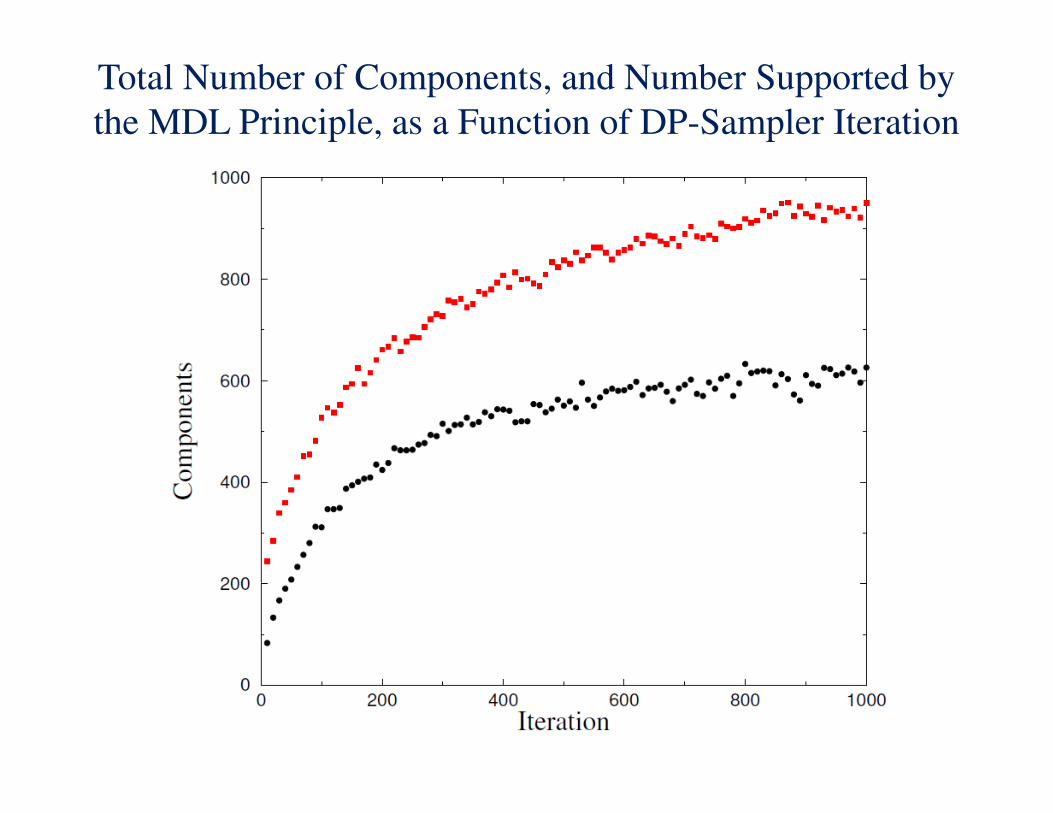
Total Number of Components, and Number Supported by
the MDL Principle, as a Function of DP-Sampler Iteration

Tradeoff Between Number of Dirichlet Components and
Decrease in Total Description Length per Amino Acid

Topographic Map of the Big Island of Hawai’i
A
A
A
A
A
A
A
A
A
A
A
A
A
A
A
A
A
A
A
A
A
A
A
A
A
A
A
A
A
A
A
A
A
Mauna Kea
Hualalai
Kohala
Mauna Loa
Kilauea

Topographic Map of Pennsylvania

Visualizing Dirichlet Mixture Components
Reorder the amino acids: RKQEDNHWYFMLIVCTSAGP
Represent the target frequency � for an amino acid by a symbol
for its implied log-odds score �� = log� �/� as follows:

A Reordered Subset of a 134-Component Dirichlet Mixture
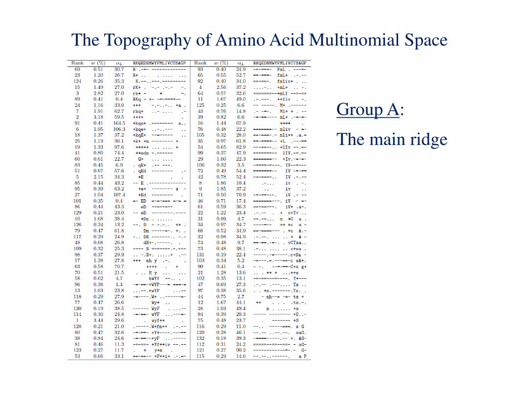
The Topography of Amino Acid Multinomial Space
Group A:
The main ridge

Another Section of the Main Ridge
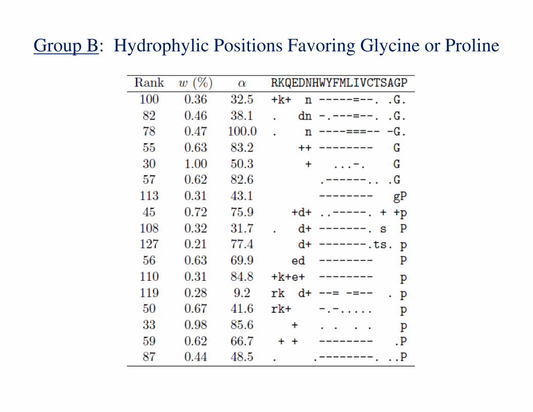
Group B: Hydrophylic Positions Favoring Glycine or Proline

Group C: Positions Favoring Single Amino Acids

Slice Sampling γ

Collaborators
National Center for Biotechnology Information
Xugang Ye
Yi-Kuo Yu
University of Maryland, College Park
Viet-An Nguyen
Jordan Boyd-Graber