The Pennsylvania State University

The Graduate School

Department of Sociology and Criminology

DISADVANTAGE AND SOCIAL RELATIONS:

SHORT- AND LONG-TERM EFFECTS OF STRATIFICATION IN SOCIAL

RELATIONS DURING ADOLESCENCE

A Dissertation in

Criminology

by

Douglas Baals

2018 Douglas Baals

Submitted in Partial Fulfillment

of the Requirements

for the Degree of

Doctor of Philosophy

August 2018

The dissertation of Douglas Baals was reviewed and approved* by the following:

Wayne Osgood

Professor Emeritus of Criminology and Sociology

Dissertation Advisor

Chair of Committee

Jeremy Staff

Professor of Sociology and Criminology

Director of Graduate Program in Criminology

Derek Kreager

Professor of Sociology and Criminology

Director of Justice Center for Research

Scott Gest

Professor of Human Development and Family Studies

*Signatures are on file in the Graduate School

iii

ABSTRACT

Disadvantage has received much attention within the fields of criminology and

education as scholars have sought to understand why individuals from lower

socioeconomic backgrounds have poorer outcomes (Cohen 1955; Hagan 1992; Coleman

1959). It is well documented that social ties during adolescence are important for the

development of human and social capital, have important consequences for adolescent

behavior, and can affect adjustment in young adulthood. This dissertation seeks to

advance our understanding of this topic by examining social relations among adolescents

as a potential mediator of the effects of disadvantage, despite adolescent social relations

being regarded as a critical in adolescents’ daily lives and important contributor to their

future success.

Using longitudinal social network data from the PROSPER Peers project, I find

that disadvantage has an effect on four measures of social relations: in-degree, Bonacich

centrality, reciprocity, and stability. The results from this dissertation indicate support

that among the reasons for this disparity in social relations are three types of factors:

school, family, and individual.

Additionally, this dissertation empirically examines the consequences of the

disparity in social relations between financially disadvantaged adolescents and non-

disadvantaged adolescents. The results demonstrate that financially disadvantaged

adolescents are more likely than non-disadvantaged adolescents to have peers who are

more disadvantaged and to have peers who engage in higher amounts of delinquency, and

that popularity mediates these relationships. Next, I find that the disparity in social

iv

relations, and the disadvantage and delinquency of friends, mediates the relationships of

disadvantage and delinquency and school instability.

Finally, a growing field of research is examining the long-term effects of

adolescent friendships, such as how the development of socioemotional traits during

adolescence may help to explain adulthood economic, educational, and health behaviors

(Bowles, Herbert, and Osborne 2001; Cunha et al. 2006). I extend this area of research

by demonstrating that popularity is a significant mediator of the relationship between

disadvantage and educational attainment in young adulthood.

v

TABLE OF CONTENTS

List of Figures ......................................................................................................................... vii

List of Tables ........................................................................................................................... viii

Acknowledgements .................................................................................................................. x

Chapter 1 Social Class, Social Relations, and Delinquency .................................................... 1

Disadvantage within Criminology ................................................................................... 4 Theoretical and Empirical Background from Criminology and Education ..................... 5 Adolescent Friendships and Social Relations .................................................................. 10

Adolescent Friendships and Short-Term Behavior .................................................. 12 Adolescent Friendships and School Instability ........................................................ 14 Adolescent Social Relations and Adulthood Adjustment ........................................ 16

Longitudinal Social Network Approach .......................................................................... 20 The Current Project .......................................................................................................... 21

Chapter 2 Data and Measures .................................................................................................. 24

PROSPER Data ........................................................................................................ 24 Measures .................................................................................................................. 27

Chapter 3 Disadvantage and Social Relations ......................................................................... 32

Methodology .................................................................................................................... 34 PROSPER Data ........................................................................................................ 34 Measures .................................................................................................................. 34 Analytic Strategy ...................................................................................................... 41

Results .............................................................................................................................. 44 Bivariate Analyses.................................................................................................... 44 Multi-level Results ................................................................................................... 48 Sensitivity Analyses ................................................................................................. 61 Supplemental Analyses ............................................................................................ 62

Discussion ........................................................................................................................ 63

Chapter 4 Disadvantage, Social Relations, and Behavior ........................................................ 84

Methodology .................................................................................................................... 86 PROSPER Data ........................................................................................................ 86 Measures .................................................................................................................. 86 Analytic Strategy ...................................................................................................... 93

Results .............................................................................................................................. 95 Bivariate Analyses.................................................................................................... 95 Multivariate Analyses .............................................................................................. 97

Discussion ........................................................................................................................ 105

vi

Chapter 5 Adolescent Social Relations and Young Adulthood Adjustment ............................ 114

Methodology .................................................................................................................... 116 PROSPER Data ........................................................................................................ 116 Measures .................................................................................................................. 117 Analytic Strategy ...................................................................................................... 123

Results .............................................................................................................................. 124 Bivariate Analysis .................................................................................................... 124 Multivariate Analyses .............................................................................................. 125 Sensitivity Analyses ................................................................................................. 128

Discussion ........................................................................................................................ 132

Chapter 6 Conclusion ............................................................................................................... 141

References ................................................................................................................................ 145

vii

LIST OF FIGURES

Figure 3-1: Path diagram demonstrating the focus of this chapter. ......................................... 33

Figure 3-2: Analytical Path Diagram based on Baron and Kenny’s (1986) Mediation

Method. ............................................................................................................................ 43

Figure 3-3: Comparison of Means Tests for In-Degree, Bonacich Centrality, Reciprocity,

and Friendship Stability by Disadvantage. ....................................................................... 47

Figure 4-1: Path diagram demonstrating the focus of this chapter. ......................................... 86

Figure 5-1: Path diagram demonstrating the focus of this chapter. ......................................... 116

viii

LIST OF TABLES

Table 3-1: Descriptive Statistics .............................................................................................. 35

Table 3-2: Comparison of Means Tests for In-Degree, Bonacich Centrality, Reciprocity

and Friendship Stability by Disadvantage, combining all eight waves of data. ............... 46

Table 3-3: 3-Level, Multilevel Models of Disadvantage Predicting In-Degree, Bonacich,

Reciprocity, and Stability. ................................................................................................ 69

Table 3-4: Disadvantage Predicting Mediating Variables. ...................................................... 70

Table 3-5: 3-Level, Multilevel Models of Disadvantage Predicting In-Degree, Bonacich,

Reciprocity, and Stability with the School Variables. ..................................................... 71

Table 3-6: Percentage of Mediation explained by School Variables. ...................................... 72

Table 3-7: 3-Level, Multilevel Models of Disadvantage Predicting In-Degree, Bonacich,

Reciprocity, and Stability with the Family Variables. ..................................................... 73

Table 3-8: Percentage of Mediation explained by Family Variables. ...................................... 74

Table 3-9: 3-Level, Multilevel Models of Disadvantage Predicting In-Degree, Bonacich,

Reciprocity, and Stability with the Other Individual Variables. ...................................... 75

Table 3-10: Percentage of Mediation explained by Other Individual Variables. ..................... 76

Table 3-11: 3-Level, Multilevel Models of Disadvantage Predicting Four Social Relations

with all Mediating Variables. ........................................................................................... 77

Table 3-12: Percentage of Mediation explained by all Variables. ........................................... 78

Table 3-13: 3-Level Overdispersed Poisson Predicting In-Degree.......................................... 79

Table 3-14: 3-Level HLM Predicting Bonacich Centrality ..................................................... 80

Table 3-15: 3-Level Binomial Model Predicting Reciprocity based on Out-Degree .............. 81

Table 3-16: 3-Level Binomial Model Predicting Stability based on Out-Degree at T1 .......... 82

Table 4-1: Descriptive Statistics .............................................................................................. 86

Table 4-2: Outcomes by Disadvantage .................................................................................... 96

Table 4-3: Baseline Multivariate Models of Disadvantage Predicting Four Outcomes. ......... 108

Table 4-4: Path a of Mediation Analysis; Mediating Variables as Outcomes. ........................ 109

Table 4-5: Disadvantage Predicting Peer Disadvantage .......................................................... 110

ix

Table 4-6: Disadvantage Predicting Peer Delinquency ........................................................... 111

Table 4-7: Disadvantage Predicting Delinquency ................................................................... 112

Table 4-8: Disadvantage Predicting School Instability ............................................................ 113

Table 5-1: Descriptive Statistics. ............................................................................................. 117

Table 5-2: Disadvantage Predicting Educational Attainment. ................................................. 137

Table 5-3: Path a of Mediation Analysis: Social Measures as Outcomes. .............................. 138

Table 5-4: Disadvantage Predicting Educational Attainment, with Social Measures as

Mediators. ........................................................................................................................ 139

Table 5-5: Disadvantage Predicting Educational Attainment, with Social Measures and

Type of Friends as Mediators. .......................................................................................... 140

x

ACKNOWLEDGEMENTS

I would like to thank my family, friends, and advisors for their support in the completion

of my project. I am very grateful for all of their insights, feedback, and assistance during this

process.

Grants from the W.T. Grant Foundation (8316), National Institute on Drug Abuse (R01-

DA018225), and National Institute of Child Health and Development (R24-HD041025)

supported this research. The analyses used data from PROSPER, a project directed by R. L.

Spoth, funded by the National Institute on Drug Abuse (RO1-DA013709) and the National

Institute on Alcohol Abuse and Alcoholism (AA14702). The content of this article is solely the

responsibility of the authors and does not necessarily represent the official views of the National

Institutes of Health.

1

Chapter 1

Social Class, Social Relations, and Delinquency

Disadvantage has received much attention within criminology as scholars have

sought to understand the class-crime/delinquency relationship (Shaw and McKay 1942;

Cohen 1955; Merton 1968; Hagan 1992). However, there has been little empirical

research devoted to exploring the indirect effects of disadvantage. Specifically, I seek to

advance our understanding of this topic by examining social relations among adolescents

as a potential mediator of the effects of disadvantage, despite adolescent social relations

being regarded as a critical in adolescents’ daily lives and important contributor to their

future success. This dissertation builds on existing knowledge by examining how one’s

social class background indirectly affects adolescent delinquency and young adulthood

adjustment through one’s adolescent social relations.

Criminology has historically places a great deal of emphasis on the influence of

friends on delinquency (Warr, 2002). Differential association theory argues that one’s

involvement in delinquency/crime depends on the balance of one’s associations, and that

individuals who associate more with delinquent individuals than non-delinquent

individuals will tend to be delinquent (Sutherland 1947). Subculture theory argues that

adolescents, specifically financially disadvantaged adolescents, who fail to gain

conventional status will create alternative norms and values to measure themselves and

join a group of peers who share those standards (Cohen 1955). Rather than attempting to

achieve the middle-class ideals, they determine their sense of worth and status by

2

delinquent actions, such as engaging in property crime and/or violence. Thus, according

to both differential association and subculture theory, one’s involvement in

delinquency/crime is largely shaped by the peers that one associates with. In other

words, the type of friends matter for whether an adolescent engages in delinquency, in

that, if an adolescent is friends with other delinquents he/she is more likely to engage in

delinquency.

This dissertation also draws insights from the literature on education and

adolescent development, which has examined how adolescent friendships contribute to

the cognitive and emotional development of adolescents. Such research has also

considered how adolescent social relations matter for young adulthood outcomes, such as

income. This dissertation examines whether adolescent social networks are pushing

financially disadvantaged adolescents to the periphery of the social networks, and, if so,

how this network structure may have a detrimental impact upon these disadvantaged

adolescents.

Figure 1.1 presents a path diagram of the empirical aims of this dissertation. At

the beginning of each empirical chapter, I will present a detailed version of Figure 1.1 to

demonstrate how that chapter fits into the overall dissertation. Drawing from

criminological and educational theories, I focus on three primary research questions.

First, what is the relationship between disadvantage and social relations, and what

potential mediators might account for that relationship? Second, does the disparity in

social success between adolescents from a disadvantaged background and those from a

non-disadvantaged background partially mediate the relationship between social class

and short-term consequences of delinquency and school instability? Third, does the

3

disparity in social success between disadvantaged adolescents and non-disadvantaged

adolescents partially mediate the relationship between disadvantage and adjustment in

young adulthood?

Figure 1.1: Path Diagram of this Dissertation.

This chapter is organized in the following manner. The first section reviews the

class-crime/delinquency relationship within criminology and discusses the need to

consider indirect effects of disadvantage. The second section discusses the theoretical

perspectives and existing knowledge on stratification and adolescent outcomes within

both criminology and education. This section elaborates on the type of factors that are

potential mediators of the class-delinquency relationship, as examined in this dissertation.

Specifically, this section reviews research on the school, family, and individual attributes

that may be related to adolescent social relations and behavior. The third section covers

the importance of and research on adolescent friendships and social

relations. Specifically, this section describes the short- and long-term effects of

adolescent social ties. The fourth section discusses how longitudinal social network data

are uniquely equipped to answer this dissertation’s research questions. This chapter ends

with an overview of the current project.

4

Disadvantage within Criminology

In the early years of criminology, the discipline was heavily focused on social

class, with many theories proposing an inverse relationship between class and criminality

(Shaw and McKay 1942; Cohen 1955; Merton 1968; Wolfgang and Ferracuti 1967;

Willis 1977). Many of these theoretical arguments seemed to be supported when relying

on official crime statistics. However, with the rise of self-report data, the class-crime

relationship became murky, with studies using self-report data failing to demonstrate the

expected relationship between social class and criminality. Tittle et al. (1978:645)

questioned the actual evidence of a class-crime relationship and argued that there are

issues of representativeness within the studies and that, due to the various methodologies,

it is difficult to reach any meaningful conclusions. Tittle et al. (1978) concluded that

either there never was an inverse relationship between social class and crime, or that the

class-crime relationship has become less important in the decades following the rise of

criminology.

However, Braithwaite (1981) questioned the work by Tittle and colleagues

(1978), and claimed that neglected evidence suggests that criminology should not be so

fast to call the class-crime relationship a myth. Braithwaite (1981:47) argued that the

operationalization of a class-crime relationship used among the studies reviewed by Tittle

and colleagues (1978) led to a biased conclusion, and that there is evidence that self-

report studies tend to exaggerate the proportion of middle-class delinquency. Similarly,

challenging the conclusion of Tittle and colleagues (1978), Clelland and Carter

(1980:331) argued that the existing research on the class-crime relationship is bound by

5

several empirical limitations and that future research “need[s] more careful thinking

about crime and more insightful thinking about class.” As criminology became more

systematic and precise, Hagan (1992:11-12) urged researchers to “acknowledge the

variety and the complexity of the relationship between class and crime.”

Dunaway, Cullen, Burton, and Evans (2000:625) stated, in line with Hagan’s

(1992) arguments, “…that criminologists should continue to refine the

conceptualizations, measures, and research techniques used, and perhaps [the] indirect

ways that class affects crime.” This dissertation seeks to advance research on the class-

crime relationship by examining the indirect effects of class on short- and long-term

outcomes via social relations during adolescence. In other words, does social class

background indirectly affect adolescent delinquency and young adulthood adjustment

through adolescent social relations?

Theoretical and Empirical Background from Criminology and Education

To answer the research questions in this dissertation, I integrate insights from

both the criminology and education literatures. Within criminology, the relationship

between class and crime is most relevant to subcultural theories. Specifically, subculture

theories argue that financially disadvantaged adolescents are differentially equipped to

gain status in educational institutions as compared to adolescents from families of higher

socioeconomic backgrounds (Cohen 1955). Cohen’s ideas were clearly evident in Willis’

(1978) ethnography of British working-class boys. The boys created their own

counterculture that celebrated fighting and conflict with the law, mocked other students

6

who did well in school, and rebelled against teachers. Several of the working-class ‘lads’

dropped out of school and took manual-labor jobs. Despite easily finding a first job,

many of the ‘lads’ soon left their working class positions and were unable to find new

employment. Hagan (1997) observed similar educational and employment difficulties

among Canadian youth. Adolescents from working-class backgrounds were more likely

to engage in delinquency, have contact with the police, and drop out of school. The

former delinquents were often unemployed years later, and reported more feelings of

hopelessness and despair. Hagan (1997:133) described the delayed feelings of despair as

a “sleeper effect,” resulting from “subcultural involvement in delinquency with the

structural consequences of prematurely leaving school and unemployment.”

A key component of subcultural theories is how working-class youth act in

school, and especially whether or not they drop out. Cohen (1955) argued that

relationships with teachers, getting into trouble, and educational aspirations may affect

how adolescents succeed. Within schools, adolescents are held to and measured by

middle-class standards, making it unlikely that disadvantaged adolescents will be able to

succeed. However, though these theories specify educational achievement, it is important

to clarify here that there is more to adolescent status than just academic success.

Specifically, social relations among students are a critical aspect of success that has not

received enough empirical attention within criminology.

The importance of the number of friends and the type of friendships one has

during adolescence plays multiple causal roles for social competence (Parker and Asher

1987). Friendships contribute greatly to the development of adolescents both cognitively

and emotionally, helping them learn cooperative skills while also providing sources of

7

comfort in times of stress. “Student-student relationships are an absolute necessity for

healthy cognitive and social development and socialization” (Johnson 1980:125).

Adolescents self-report that they spend more time talking to their peers than any other

single activity and that they are happiest when doing so (Csikszentmihalyi, Larson, and

Prescott 1977). Additionally, research has demonstrated that social support helps

adolescents deal with life stress (Cassell 1973; Caplan 1974; Dean and Lin 1977). From

a social capital perspective, having in-school friends allows adolescents to access

additional resources, such as study groups, and receive help navigating the school context

(Crosnoe, Cavanagh, and Elder 2003).

It is evident in the literature that adolescent friendships are non-randomly formed,

based on individual characteristics and guided by opportunities and attractiveness

(Rivera, Soderstrom, and Uzzi 2010; Crosnoe 2000). One of these individual

characteristics is the socioeconomic background of the adolescent. My first task will be

to determine a baseline association between disadvantage and friendship formation.

Next, I go further to advance understanding of the nature of this relationship in terms of

the mediators that contribute to it. To understand how socioeconomic background may

be influencing friendship formation, it is important to discuss potential mediators the type

of factors that may contribute to the social component of adolescent status. The

formation of, and the consequences of, these social ties is the focus of the current

dissertation.

Researchers have identified a number of factors that matter for the social relations

of adolescents. Coleman (1959) explained that adolescents take academic factors into

account in choosing their friends, but place priority on topics outside of academics as

8

well. The academic component includes factors such as school performance and attitudes

towards school.

In addition to school-related attributes, family characteristics such as family

relations, parental communication, family home condition and location, and parental

school involvement may have important roles in the selection of friends. Socioeconomic

status is also an important predictor of family relations, parental communication, family

home condition, family location, and parental school involvement. Further each of these

variables can influence adolescent friendship formation, therefore may be mediating the

relationship between disadvantage and social success. Parents influence friendship

formation by monitoring youth activities and the type of peer-interactions that they have

(Crosnoe 2000; Parke and Bhavnagri 1989), and communicating the traits of positive

peer relations to their children. Even as adolescents increasingly spend time outside of

their parents’ monitoring, children often learn from their parents’ judgments about who

they should spend time with (Cohen 1955). Related to this, economic disadvantage alters

how parents interact with and monitor their children (Crosnoe, Mistry, and Elder 2002;

Thomson, Hanson, and McLanahan 1994; Elder, Nguyen, and Caspi 1985; Elder et al.

1992). Home condition and location may also play an important role in the selection of

friends. Even as young as sixth grade, adolescents are able to distinguish peers’ class by

characteristics of their family and the home that they had (Cohen 1955). Additionally,

parental involvement in the child’s school and community can help positively shape

children’s social competence (Parke and Bhavnagri 1989; Hill and Craft 2003; Hill and

Taylor 2004). However, parents of a lower socioeconomic status are less likely to be

9

involved in school-related activities than parents of a higher socioeconomic status (Hill

and Taylor 2004:162).

Finally, individual attributes, such as mental and physical health, attractiveness,

bullying, and confidence/nervousness may play important mediating roles in the

relationship between disadvantage and social success. Physical and mental health are

important when considering how adolescent friendships develop (Bronfenbrenner and

Morris 2006; Simpkins Schaefer, Price, and Vest 2013), and health in adolescence has

been shown to be associated with one’s social class (Starfield, Riley, Witt, and Robertson

2002). Additionally, research has demonstrated that adolescent culture places high

importance on attractiveness (Coleman 1959; Alder and Alder 1998), which also may be

associated with disadvantage.

In sum, many of the factors that affect adolescent friendships (Crosnoe 2000:381)

are related to an adolescent’s socioeconomic background and, thus, may be constraining

financially disadvantaged adolescents’ ability to socially succeed. It is clear that three

categories of potential mediators emerge within the literature: school factors, family

factors, and other individual attributes. The current project will examine five variables

from each of these three groups to determine how each grouping of variables may

mediate the relationship between disadvantage and social relations. This is an important

area of research that deserves further empirical attention as decades of research has

demonstrated how important friendships are during adolescence.

10

Adolescent Friendships and Social Relations

Friendships and social success can be considered in a number of ways. I am

going to distinguish between two main aspects of adolescents’ position or status in their

schools’ friendship networks: popularity and quality of friendships. Popularity is their

prominence in terms of the extensiveness of their connections. I am going to look at that

in two ways. First, I am going to examine how many friendship choices they attract from

other students. Second, I am going to use an indicator, called Bonacich centrality, which

weights the friendship connections by the prominence of the friends who choose them.

The second index gives a richer sense of their standing in the larger hierarchy of the

schools’ friendship networks.

Beyond popularity, the quality of the friendships should also be considered as

they have been shown to impact feelings of belonging (Hartup 1996). Berndt (2002:7)

described friendship quality as “high levels of prosocial behavior, intimacy, and other

positive features, and low levels of conflicts, rivalry, and other negative features.”

Researchers have examined the consequences of a number of indicators of friendship

quality. Giordano et al. (1998) found greater levels of intimacy with adolescent friends to

be related to a number of adulthood outcomes, including higher self-esteem and marital

satisfaction. Allen, Schad, Oudekerk, and Chango (2014) found adolescent

pseudomature behaviors (e.g. delinquent acts and precocious romantic activity) to be

inversely related to quality of adolescent peer relationships as well as young adulthood

adjustment. The authors suggest that “pseudomature behaviors might lead to future

difficulties because these pseudomature behaviors replace efforts to develop positive

11

social skills and meaningful friendships and thus leave teens less developmentally mature

and socially competent over time” (Allen et al. 2014:11). Also, “[e]stablishing oneself as

a socially desirable companion with one’s adolescent peers appear[s] most strongly

predictive of qualities of relationship functioning in adulthood” (Allen, Chango, and

Szwedo 2014:11).

Additionally, friendship mutuality and friendship stability are important

protective factors against behavioral, emotional, and/or social problems in adolescence

(Bukowski, Hoza, and Boivin 1994; Waldrip et al. 2008). “Close friendships provide

adolescents with developmentally salient opportunities to improve their social skills and

social competence” (Smetana, Campione-Barr, Metzger 2006; Collins and Steinberg

2005). Thus, due to the importance of reciprocity and stability upon one’s self-esteem

and belonging, qualitative features of friendships should be considered in addition to

number of friends and overall popularity.

Reciprocity is an important aspect of friendship quality to consider because

mutual friendships have greater importance for the development of adolescents

(Bukowski et al. 1994), while failed one-way ties (i.e. non-mutual friendships) may lead

to adverse effects, such as lower self-esteem, embarrassment, and/or depression (Rivera,

Soderstrom, and Uzzi 2010). Vaquera and Kao (2008) argued that friendship reciprocity

is especially important when considering one’s social support during adolescence,

concluding that friendship reciprocity has strong effects on feelings of school belonging

and educational outcomes. Cauce (1986) found that the number of reciprocated friends in

one’s social group has an effect on school and peer competence.

12

The stability of friendships is another important aspect of friendship quality.

Stable friendships during adolescence have important ramifications for self-esteem and

altruism (Berndt 1982). Additionally, stable friendships can offer feelings of closeness,

validation, and acceptance ((Bukowski et al. 1994). Bukowski and colleagues (1994)

went on to explain that there is a strong association between friendship stability and

quality, and that a high turn-over in friendships will also mean friendships of lower

quality. Similarly, transitory friendships are going to be less meaningful and helpful than

enduring ones.

Adolescent Friendships and Short-Term Behavior

The second topic I address in this dissertation is the role of adolescent social

relations on near-term outcomes, including delinquency and school instability. This

section covers the relationship between friendships and delinquency, and the next section

will discuss school instability. Friendships and social success may have important

ramifications for antisocial behavior, such as delinquency, increased interaction with

delinquent peers, and school instability. Crosnoe (2000) explained that the structure of

one’s social network can influence and impact the individuals beyond the characteristics

of the network members. Similarly, studies of “…conformity to group pressure suggest

that children’s social networks might increasingly influence their attitudes and behaviors,

as well” (Crosnoe 2000:380; Berndt 1979; Costanzo and Shaw 1966). If adolescent

social networks are pushing financially disadvantaged adolescents to the periphery of the

social networks, then this network structure may have a detrimental impact upon these

13

disadvantaged adolescents. Indeed, the field of criminology has multiple theoretical

arguments as to how patterns of social network structure and individual social relations

may influence delinquency.

According to theorists such as Merton (1938), Cohen (1955), and Cloward and

Ohlin (1960), disadvantaged adolescents who fail to gain conventional status will instead

create alternative norms and values to measure themselves (Davies 1999). Rather than

attempting to achieve the middle-class ideals, they determine their sense of worth and

status by delinquent actions, such as engaging in property crime and/or violence.

“[Y]outh form oppositional groupings built around delinquent behavior as a means of

counteracting status anxieties and frustrations” (Hagan 1997:120). In other words,

disadvantaged adolescents who struggle to socially succeed may be more likely to turn to

delinquency and delinquent peers as a response.

“According to [differential association], youth learn criminality in primary

groups, such as groups of friends, but these groups are shaped by social organization”

(Crosnoe 2000:381; Sutherland 1947). Thus, based on the stratification of adolescent

social networks that is evident in the literature, and drawing from the two criminological

theories discussed above, it is likely that social status is an important mediator of the

relationship between disadvantage and individual delinquency, as well as disadvantage

and having delinquent peers. Also, it is rather clear how differential association theory

would argue that one’s social relations may lead to delinquent involvement. First,

differential association theory specifies that one’s involvement in delinquency/crime

depends on the balance of one’s associations, and that individuals who associate more

with delinquent individuals than non-delinquent individuals will tend to be delinquent.

14

Thus, according the theory, one’s involvement in delinquency/crime is largely shaped by

the peers that one associates with. In other words, the type of friends matter for whether

an adolescent engages in delinquency, in that, if an adolescent is friends with other

delinquents he/she is more likely to engage in delinquency.

Within research of adolescent social networks, it is evident that aggressive and/or

delinquent children tend to be on the periphery of their social networks (Coie, Dodge, and

Coppotelli 1982; McGuire 1973). Thus, if adolescents from disadvantaged backgrounds

are forced to withdraw to the periphery of their social networks, then they are likely to be

restricted in what individuals they are able to select as friends, while arguably are more

likely to come into contact with other rejected adolescents (Light and Dishion 2007). In

other words, they are more likely to associate with violent and/or maladjusted peers than

adolescents who are central within their social network. So, because disadvantaged

adolescents will be less likely to socially succeed than advantaged adolescents,

disadvantaged adolescents should be more likely to be in contact with delinquent and/or

violent peers. Furthermore, due to their restricted pool of friends to choose from,

disadvantaged adolescents should be more likely to form their primary friendships with

these delinquent and maladjusted peers.

Adolescent Friendships and School Instability

Next, I address another important consequence of one’s social ties, school

instability. Elements of social integration are at the forefront of theoretical research of

student mobility and dropout within the field of education. Wehlage et al. (1989)

15

highlighted the importance of the social dimension of school belonging, arguing that

social ties, in addition to academic performance, affect one’s likelihood of dropping out

of school. Parker and Asher (1987) had a similar argument, concluding that social

success during adolescence increased the likelihood of graduating from high school.

Wehlage et al (1989) went on to explain that disadvantaged students, specifically, may

need additional help in both social engagement and academic engagement to succeed in

school. Therefore, as financially disadvantaged adolescents are unlikely to succeed

socially, and are more likely than non-disadvantaged adolescents to experience school

instability, it seems that social relations may be an important mediator of the relationship

between disadvantage and school instability.

While most research examining school withdrawal, especially in criminology,

focuses solely on school dropout as an outcome, Rumberger and Larson (1998) stated

that school mobility is important to consider, as well. In fact, Rumberger and Larson

(1998) concluded that school mobility may be considered a risk factor for future dropout,

as students in their sample who transferred schools just once between 8th and 12th grade

were twice as likely as students who did not transfer schools to experience future

dropout. Thus, rather than only considering school dropout as a consequence of

educational disengagement, school dropout and school mobility (i.e., school instability)

should be considered.

16

Adolescent Social Relations and Adulthood Adjustment

The final topic I address in this dissertation is how adolescent social relations are

related to educational attainment in young adulthood. While school grades are an

obvious and well documented mediator, recent research has suggested that adolescent

social relations may also help explain the relationship between disadvantage and young

adulthood adjustment. As discussed previously, adolescents from a disadvantaged

background are less likely to succeed socially within school. Additionally, it is evident in

research that disadvantaged adolescents are less likely to attain a college degree (Sewell

and Shah 1967). Thus, adolescent social relations may be partially mediating the

relationship between disadvantage and college attainment. “If peers contribute

substantially to the socialization of social competence, it follows that low-accepted

children might become more vulnerable to later life problems” (Parker and Asher

1987:358).

A growing field of research is examining the long-term effects of adolescent

friendships, such as how the development of socioemotional traits during adolescence

may help to explain adulthood economic, educational, and health behaviors (Bowles,

Herbert, and Osborne 2001; Cunha et al. 2006). Several studies have shown that

popularity and friendships during adolescence are connected to outcomes in young

adulthood, such as life adjustment (Bagwell, Newcomb, and Bukowski 2008) and income

(Shi and Moody 2017). Shi and Moody (2017) found that each additional friendship

nomination during adolescence yields an earnings increase of 1.7% fifteen years later.

This “popularity effect” is after accounting for numerous factors that might drive both

17

popularity and adult workplace success, such as educational success and personality traits

(Shi and Moody 2017).

This finding is consistent with labor market research indicating that employers are

valuing socioemotional traits like collaboration and creativity beyond standard measures

of cognitive ability (Shi and Moody 2017). Sawyer (2017) discussed that “group genius”

has become widely valued in today’s labor market; that while previously individual

creativity and intelligence were most valued, recent research is concluding that

collaboration is what drives innovation and success.

Connecting this back to this popularity effect, having more adolescent friendships

may help individuals develop skills useful for workplace collaboration. Navigating

between numerous friendships may help an individual later in life when interacting with

various workgroups. Also, easing tensions between friends may help one in the future

when navigating tensions between colleagues (Shi and Moody 2017). “Interactions with

friends can serve as a foundation for egalitarian relationships with colleagues, neighbors,

or spouses in adulthood” (Berndt 1982:1448; see Piaget 1932; Youniss 1980). Because

of consistent similarities between labor market practices and educational practices

(Seltzer and Bentley 1999; Craft, Jeffrey, and Leibling 2001), it seems likely, then, that

adolescent social relations may have important ramifications for success in the university

setting. So, similar to the findings for income (Shi and Moody 2017), popular

adolescents and/or adolescents with higher quality friendships may be provided with an

advantage in succeeding in college due to the development of socioemotional traits.

Though definitions of student success in college can vary, “[m]any consider

degree attainment to be the definitive measure of student success” (Kuh and colleagues

18

2006:5). While I am not arguing that this definition of student success is better or worse

than other definitions (e.g., college persistence, degree satisfaction), I will use degree

attainment as the sole measure of educational success in my dissertation. Understanding

the factors that contribute to educational attainment is an important area of research that

has received a lot of attention.

Interest in attending college is near universal (Kuh and colleagues 2006), but

adjustment to and succeeding within college is dependent on numerous factors. Though

academic ability is important, less than 25% of the students who start college and fail to

complete their degree are dismissed for poor academic performance (Kuh and colleagues

2006), indicating that most of the students leave for reasons other than grades. Tinto’s

(1975) theoretical framework argues that both academic and social integration is

important for college success. While Tinto’s (1975) propositions are among the most

cited and most prominent theoretical arguments in this area of research (Braxton,

Sullivan, and Johnson 1997), only a few of them have received empirical support

(Braxton, Milem, and Sullivan 2000). One of the supported propositions is that students’

entry characteristics (e.g., family background and academic ability) affect their initial

commitment to college, which influences subsequent levels of commitment (Braxton,

Milem, and Sullivan 2000).

However, Braxton and colleagues (2000) explained that additional empirical

attention is needed for the construct of social integration. Relatedly, there is some

empirical evidence that social integration is a stronger predictor of college persistence

than academic integration (Braxton, Sullivan, and Johnson 1997). “The most important

criterion for staying in college is the student’s social support network” (Skahill 2002:39;

19

Rosenthal 1995). Additionally, many researchers argue that in order for students to be

successful in college, they must learn to negotiate new environments and interact with

unfamiliar people (Kuh and Love 2000). Empirical research in this area has focused on

one’s social networks while in college, demonstrating that friendships with other students

and with faculty members matter for college success (Skahill 2002). However, as

mentioned above, friendships and social acceptance during adolescence pave the way for

one’s ability to successfully socialize in adulthood (Berndt 1982). Therefore, I argue that

additional empirical attention that links adolescent social acceptance to young-adulthood

educational attainment is needed. This is especially true for the relationship between

disadvantage, adolescent social status, and educational attainment. If most college

students that leave school are doing so for reasons other than academic performance, and

the ability to socialize is one of these factors, then adolescent social acceptance may be

an important mediator of disadvantage and educational attainment.

Additionally, it is unclear if peer acceptance is the only aspect of social relations

that affects future adjustment, or if other social measures (e.g., stability, reciprocity), as

well as the type of friends (e.g., levels of disadvantage and/or delinquency) also have an

impact. Staff and Kreager (2008) highlighted the importance of considering the type of

friends one has when examining the effects of friendships. Staff and Kreager (2008)

explained that friendships are generally linked to positive outcomes, such as an increase

in the likelihood of completing high school. However, drawing from subcultural theories

of juvenile delinquency, they argued that examining the types of friendships that one has

may have important consequences, especially for disadvantaged adolescents. Staff and

Kreager (2008) demonstrated that disadvantaged adolescents with high status in violent

20

groups are at a greater risk of dropping out of high school, and that status within violent

groups during adolescence reduces the likelihood of college completion. In other words,

it is evident that the type of friends one is socially accepted by may be important when

considering the overall effects of friendships. Therefore, my research will not only

examine social ties, but also the type of social ties disadvantaged and non-disadvantaged

adolescents are forming.

However, there are very few studies examining these relationships. The limited

amount of research on this topic may be a result of prior methodological or data

limitations; the longitudinal social network data used in this research is uniquely

equipped to address the relationship between adolescent social relations obtaining a

university degree.

Longitudinal Social Network Approach

Longitudinal social network data are necessary to effectively examine if

financially disadvantaged adolescents are differentially equipped to compete socially in

school. Social network data involve a theoretically or conceptually defined group of

individuals and information on a relation between those individuals. “Networks are a

way of thinking about social systems that focus our attention on the relationships among

the entities that make up the system, which we call actors or nodes” (Borgatti 2013:1-2).

Longitudinal social network data are especially important, as social networks are

dynamic and consistently evolving over time. “One fascinating aspect of the social

process is the continual realignment of groups, the migration of individuals from one

21

group to another…” (Cohen 1955:53). Thus, tracking social relations over time is

necessary to determine what factors may be contributing to stratification within social

networks. Utilizing longitudinal social network data allows me to assess all of the

various aspects of social integration that the literature emphasizes: number of friends,

popularity, the mutuality of friendships, and the stability of friendships. Using social

network data, and being able to use social ties, also helps alleviate bias associated with

self-reported popularity measures (Kreager 2007; Young, Barnes, Meldrun, and

Weerman 2011). In other words, social network data provides directed friendship ties

that identify which students are friends, and provide a direct method to measure friends’

characteristics and behavior.

The Current Project

As discussed above, it is well documented that social ties during adolescence are

important for the development of human and social capital, have important consequences

for adolescent behavior, and can affect adjustment in young adulthood. It is valuable,

then, to consider theoretical arguments from subculture theories that adolescents from

disadvantaged backgrounds are less likely than non-disadvantaged adolescents to be well

integrated in their school-based social networks. If adolescent social success is important

for both short- and long-term consequences, then it is important to ask, why are

disadvantaged adolescents less likely to socially succeed? Thus, this is the first research

question of my dissertation. My first task will be to determine a baseline association

between disadvantage and friendship formation. Next, I go further to better understand

22

the nature of this relationship in terms of the mediators that contribute to it. The

literature reviewed in Chapter 1 implies that the reasons for this lack of social success fall

under three categories: school, family, and individual. In Chapter 3, I address this first

research objective, examining the extent to which these three types of factors mediate the

relationship between disadvantage and social relations.

Next, the second objective of this dissertation is to determine the effects of the

stratification evident in adolescent social ties. Chapter 4 of this dissertation empirically

examines these consequences in two parts. First, if financially disadvantaged adolescents

tend to be less well integrated within their school-based social networks, then does this

have an effect on the types of friends that they do have? Second, do these social patterns,

and the types of friends gained, have a mediating impact on the relationships between

disadvantage and delinquency and school instability? As previously discussed,

subcultural theories of delinquency argue that disadvantaged adolescents who are poorly

socially integrated will be more likely to become friends with other disadvantaged or

maladjusted adolescents. Chapter 4 examines if financially disadvantaged adolescents

have more disadvantaged and/or delinquent friends than non-disadvantaged adolescents.

If so, I will then test if disparities in social measures mediate these relationships. Then,

to address my second research question, I will examine if adolescent social relations, and

types of friends, mediate the relationships of disadvantage and delinquency and school

instability.

Finally, the third objective of this dissertation is to determine if adolescent social

relations partially mediate the relationship between disadvantage and educational

attainment. As discussed above, studies have shown that popularity and friendships

23

during adolescence are connected to outcomes in young adulthood, such as life

adjustment (Bagwell, Newcomb, and Bukowski 2008) and income (Shi and Moody

2017). Additionally, there is a clear and persistent relationship between disadvantage and

educational attainment. Though much of this relationship has been explained, I argue

that another cause of this relationship is the lack of social integration of disadvantaged

students during adolescence. Thus, Chapter 5 of this dissertation will empirically

examine if adolescent social relations are partial mediators of the relationship between

disadvantage and college attainment. Lastly, Chapter 6 will discuss the implications of

this dissertation’s main findings.

24

Chapter 2

Data and Measures

PROSPER Data

My dissertation will use social network data from the evaluation of the

PROmoting School-community-university Partnerships to Enhance Resilience

(PROSPER) longitudinal study (Spoth et al. 2007). This data set was collected using in-

school surveys from two consecutive cohorts of adolescents in 28 rural and semi-rural

communities in Pennsylvania and Iowa, with the populations of these communities, based

on the 2000 census, ranging from 6,975 to 44,510 (Spoth et al. 2007). These

communities were matched on school district size and location, and then half of the

districts were randomly selected to receive an intervention program, with the other

districts serving as the comparison condition. Eligible school districts that participated in

the study contained between 1,300 and 5,200 students, with at least 15% of the students

qualifying to receive free or reduced-cost school lunch, and at least 95% of the students

in each school spoke English. Data collection began in the fall of the cohorts’ sixth grade

and continued in the spring of each year through twelfth grade, resulting in eight waves

of data.

In-school data collection. Data was collected in classrooms by a member of the

research staff during one class period without a teacher being present. The target sample

was every student enrolled who spoke English and did not have severe cognitive

25

disabilities. Students who joined the participating school districts were added to the

sample at the year of joining, while those leaving the school districts remained in the

sample only for the waves that they were present. Students and their parents did have the

option to opt out of the sample at each wave. The sample size consists of approximately

9,000 students at each wave, with participation rates averaging approximately 88% across

all eight waves. The questionnaire asked students about a variety of topics, such as

delinquency, substance use, family relations, and school bonding.

In addition to the importance of this being a longitudinal data set, this data source

is well suited to my dissertation because it provides social network data. At each wave of

data collection, students were asked to name up to two best friends and five additional

close friends in their current grade and school. These friendship nominations were then

matched to the student rosters, allowing researchers to create a full social network of the

cohort, alleviating bias associated with self-reported popularity measures (Kreager 2007;

Young, Barnes, Meldrun, and Weerman 2011). In other words, these questions produced

directed friendship ties that identify which students are friends, and provide a direct

method to measure friends’ characteristics and behavior. Students, on average, named

four friends per wave, and 82% of nominations were matched successfully to other

students on class rosters. Friendship nominations could not be matched if nominations

were not on the class roster or if there were multiple plausible names. One of the 28

communities did not allow collection of friendship data, so that community is excluded in

my analyses.

In-Home Subsample. While collecting the in-school sample, a random subsample

of 2,267 students from the first cohort were invited to participate in a longer interview

26

conducted at the student’s home, which included interviews with the students and the

students’ parents. These in-depth interviews continued through grade nine (total of five

waves of data). This in-home dataset is important for my dissertation because it includes

additional variables of the students and the students’ families, such as household location,

household condition, and parental school involvement. Of the 2,267 students invited to

participate, 980 (43%) participated in at least one wave (average of three waves per

student). When using the in-home sample, I will be using waves 1 through 5. I

compared mean disadvantage from the in-home sample to the in-school sample, and there

are no statistically significant differences between the two samples.

Follow-up Subsample. Finally, the PROSPER Peers project includes follow-up

interviews at approximately 24 years of age for a subsample of adolescents. These

follow-up interviews are important for this dissertation as it allows for the examination of

the long-term consequences of adolescent social relations, specifically related to

educational attainment. The first empirical chapter of my dissertation will primarily use

the in-home data set for the bulk of the analysis, as the in-home sample includes

additional theoretically important variables that were not part of the in-school

questionnaire. The second empirical chapter of my dissertation will primarily use the in-

school sample as this chapter will be addressing type of friends and individual behavior

across all eight waves of the sample. Finally, the third empirical chapter will use both the

in-school sample and the follow-up sample. I will use the in-school data to create high

school averages of popularity, stability, and reciprocity, as well as high school averages

of control variables. Then, I will supplement this data with the follow-up data to use

educational attainment as my dependent variable.

27

Measures

This section broadly describes the measurement of social and disadvantage

variables used in this research. Drawing from the literature on how to best measure these

concepts, detailed descriptions are included below and then descriptive statistics and brief

descriptions are provided in each empirical chapter of the respective analyses.

Social Measures

In-Degree. In-degree centrality is the number of nodes (i.e., individuals) who

nominated a respondent as a friend. In other words, when dealing with friendship data,

in-degree centrality counts the number of friendship nominations that an individual

receives from others (in-degree). In-degree centrality is an important indicator of an

individual’s standing within a social network, which has played a central role in research

on adolescence social relations (Kreager and Staff 2009; Staff and Kreager 2008).

Further, because it is based on other respondents’ friendship choices, it is not subject to

the biases of self-reported popularity measures. For this dissertation, I use in-degree

centrality as an outcome variable in Chapter 3.

Bonacich Centrality. Bonacich centrality provides additional information that is

relevant to one’s overall popularity (Borgatti 2013). Bonacich centrality is a function of

the prestige of the nodes that a given node is connected to. In other words, each tie of a

given node is weighted based on the centrality of the people that the node is tied to. For

this dissertation, the Bonacich centrality calculations used a weight parameter of

0.75*largest normed eigenvalue, as the weight parameter can be no larger than the largest

28

normed eigenvalue of the network. Bonacich centrality serves as an outcome variable in

Chapter 3 and as a mediating variable in Chapters 4 and 5.

Reciprocity. Because complete social network data includes information from

everyone within the network, I am able to assess the reciprocity (i.e., mutuality) of each

individual’s friendship nominations. Reciprocity is measured by counting the number of

reciprocated nominations, relative to the number of nominations sent. At times in this

dissertation, this is calculated as a proportion, computing as the number of reciprocated

friendships divided by the number of sent nominations. For this dissertation, I use the

number of reciprocated nominations as an outcome variable in Chapter 3, and then

reciprocity rate as a mediating variable in Chapters 4 and 5.

Stability. Additionally, by using longitudinal social network data, friendship

nominations can be tracked from one year to the next to determine the overall stability of

each individual’s friendships. Friendship stability is measured by counting the number of

received nominations that repeat from T1 to T2, while accounting for the total number of

nominations received in T1. At times in this dissertation, friendship stability is converted

to proportion, dividing the number of repeated nominations received in T2 by the number

of nominations received in T1. Similar to reciprocity, I use the number of stable

friendships as an outcome variable in Chapter 3, and the rate of stable friendships as a

mediating variable in Chapters 4 and 5.

29

Disadvantage

In addition to the importance of the longitudinal social network data that the

PROSPER project contains, the PROSPER data set allows me to examine different

aspects of disadvantage. Research examining a child’s socioeconomic status argues that

there is more to measure than just economic problems, concluding that there are three

elements of a child’s socioeconomic background that should be considered: financial

capital, social capital, and human capital. Each of these elements can have important

consequences for a child’s adjustment. “For children, what parents do and what parents

afford by way of physical, social, and material resources both internal and external to the

family are presumed to be among the major paths connecting SES to adaptive

functioning” (Bornstein and Bradley 2014:3). When operationalizing the socioeconomic

status of an adolescent, Entwisle and Astone (1994) explain that it is most effective to use

household income (financial capital), mother’s education (human capital), and if the child

the lives in a two-parent household (social capital). In addition to these three measures of

disadvantage, a fourth method to operationalize disadvantage is to use a measure of free

or reduced-price lunch (FRL), though the effectiveness of this measure has been

questioned (Hauser 1994; Entwisle and Astone 1994). More specifically, Sirin (2005)

argued that adolescents are less likely to receive FRL as they get older, even if they

qualify for it, due to worries of stigma. A second reason this variable is criticized is

because of using a binary variable to measure such a complex concept (Harwell and

LeBeau 2010).

30

Osgood, Baals, and Ramirez (unpublished) use the PROSPER data to compare the

effectiveness of using FRL as a measure of disadvantage to three other measures of an

adolescent’s socioeconomic background: household income, mother’s education, and

household composition. In the PROSPER study, at each in-school wave, students were

asked what they did for lunch on school days. Adolescents who indicated that they

receive a free or reduced-price lunch (FRL) were coded as 1 for that wave, with everyone

else being coded as 0. Additionally, to account for the non-response patterns and obtain a

more differentiated rather than binary measure, they use the longitudinal aspect of the

PROSPER data to create an aggregate measure of FRL using empirical Bayes shrinkage

estimates from HLM. This continuous measure uses all available data for the adolescents

to capture their disadvantage. Osgood et al. (unpublished) place a greater emphasis on

students who are eligible for FRL across multiple waves, and on students receiving FRL

in later waves of the study (when it is less common). Each student is given a constant

empirical Bayes FRL score of disadvantage across all eight waves of the sample.

Osgood, Baals, and Ramirez (unpublished) compare the empirical Bayes estimate of FRL

to three other measures of an adolescent’s socioeconomic background and conclude that

it operates rather similarly to measures of household income, mother’s education, and

household composition. Additionally, Osgood et al. (unpublished) demonstrate that the

empirical Bayes FRL measure is more strongly related to outcomes and correlates than

the current wave dichotomous FRL measure.

For the purposes of this dissertation, I will use this empirical Bayes FRL measure

as my primary measure of disadvantage. Though the in-home surveys collected

information regarding parental educational and family income, Chapters 4 and 5 of this

31

dissertation use the in-school sample and the follow-up sample, respectively. In these

samples, many respondents were not part of the in-home sample, so Bayes FRL is the

best available measure of disadvantage. Therefore, to maintain a consistent measure of

disadvantage throughout this dissertation, I use the Bayes FRL as the primary measure of

disadvantage throughout.

When feasible, I also completed supplemental analyses using the three other

indicators of disadvantage to alleviate any potential concerns that relying on the Bayes

FRL measure distorted results. The first of these three is my indicator of financial

capital, which is household income before taxes for a given year, as reported by a parent

during the in-home interview. To account for the skewed distribution, I take the natural

logarithm of the income variable for my analyses. I measure human capital as the

mother’s highest level of education, as reported by a parent during the in-home interview.

Mother’s education is coded as 1 = less than H.S. diploma, 2 = high school diploma, 3 =

some college/associate’s degree, 4= B.S., B.A., or some education beyond a Bachelor’s

degree, and 5 = Graduate degree. Social capital is measured by whether or not the

adolescent lives with both biological parents, as reported by the student at each wave, and

is coded as 1 if the child lives with both biological parents and 0 if not. In addition to

using each of these variables separately, I standardized these three variables and used

them to create a composite variable of SES. The analyses in Chapter 3 were repeated

using these three disadvantage variables, as well as with the composite variable of SES,

and are presented as supplemental analyses at the end of Chapter 3.

32

Chapter 3

Disadvantage and Social Relations

Social ties during adolescence are important for the development of human and

social capital, have importance consequences for adolescent behavior, and can affect

adjustment in young adulthood. Therefore, it is important to consider that adolescents

from disadvantaged backgrounds are less likely than non-disadvantaged adolescents to be

well integrated in their school-based social networks. This chapter addresses my first

research question: why are disadvantaged adolescents less likely than non-disadvantaged

adolescents to socially succeed? This is the first link for the mediation effects of

disadvantage that I will explore in the other empirical chapters. To reiterate, subcultural

theories of delinquency argue that disadvantaged adolescents are less likely to socially

integrate into school-based social networks (Cohen 1955; Willis 1978). Though these

theories speculate on why this might be, this area of research has received little, if any,

empirical attention.

The literature reviewed in Chapter 1 implies that the reasons for this lack of social

success fall under three categories: school, family, and individual. In the current chapter,

I explore the extent to which these three types of factors mediate the relationship between

disadvantage and adolescent social relations. In addition to popularity, research has also

demonstrated the importance of examining qualitative features of friendships. Therefore,

this chapter focuses on in-degree, Bonacich centrality, reciprocity, and stability. Figure

33

3.1 displays a path diagram illustrating the focus of this chapter, which is an elaboration

of the path diagram presented in Chapter 1.

Figure 3-1: Path diagram demonstrating the focus of this chapter.

I hypothesize that financially disadvantaged adolescents will have weaker social

relations, and that this relationship can be partially explained by three broad types of

mechanisms. The first category I include consists of school variables, such as school

performance and attitudes towards school. Second, family factors, including

characteristics such as family relations, parental communication, family home condition

and location, and parental school involvement may have important roles in the selection

of friends. Third, individual factors that may be relevant include characteristics such as

mental and physical health, attractiveness, bullying, and confidence/nervousness. As

discussed in detail in Chapter 1, I chose these specific measures based on research that

demonstrates that these variables are associated with socioeconomic status, while also

being associated with adolescent friendships. For example, previous research has

demonstrated that physical and mental health are important when considering how

adolescent friendships develop (Bronfenbrenner and Morris 2006; Simpkins Schaefer,

Price, and Vest 2013), while separate research has also demonstrated that health in

adolescence is associated with one’s social class (Starfield, Riley, Witt, and Robertson

34

2002). Therefore, it seems likely that health is a mediator of the relationship between

financial disadvantage and adolescent social relations.

Methodology

PROSPER Data

The current chapter will primarily use the in-home sample from the PROSPER

Peers project. As discussed previously (see Chapter 2: Data of this dissertation), the in-

home survey began in wave 1 and continued through wave 5 (ninth grade), consisting of

980 individuals (43% response rate). The in-home survey collected more in-depth

information of the various factors that may be mediating the relationship between

disadvantage and social relations. When estimating multivariate analyses, I will use

individuals who participated in the in-home sample (n=908) so that I am able to include

the additional measures that the in-home survey offers when examining the relationship

between disadvantage and the four social relations.

Measures

Table 3.1 provides a description and descriptive statistics for all of my measures

used in this chapter. The measures of disadvantage and the four social relations use both

the in-school and in-home sample. I use the in-school sample (n=73,018) for bivariate

analyses so that I am able to examine the social relations across all eight waves of data,

which I discuss in more detail below in my analytic strategy. Thus, these measures are

35

listed twice in the table, listing the descriptive statistics for the in-home sample and the

in-school sample.

Table 3-1: Descriptive Statistics

Variable Description Mean S.D. Min Max

Emp. Bayes FRL, In-Home Empirical Bayes aggregate

of student-reported receiving

of free/reduced price lunch.

-0.15 1.70 -1.70 3.43

Emp. Bayes FRL, In-School -0.17 1.62 -1.75 3.43

Social Network Measures

In-Degree, In-Home Number of friendship

nominations received.

3.88 2.85 0 16

In-Degree, In-School 3.35 2.67 0 20

Bonacich Cen., In-Home Function of the prestige of

the nodes that a given actor

is connected to.

0.83 0.56 0 3.45

Bonacich Cen., In-School 0.77 0.58 0 4.54

Reciprocity Rate, In-Home Proportion of mutual to non-

mutual friendships.

0.53 0.33 0 1

Reciprocity Rate, In-School 0.51 0.34 0 1

Stability Rate, In-Home Proportion of friends from

T1 that overlap to T2.

0.45 0.29 0 1

Stability Rate, In-School 0.41 0.30 0 1

School Measures (In-Home)

Grades Student-reported school

grades.

4.23 0.82 1 5

School Bonding Average of eight items about

feelings towards school and

teachers.

3.96 0.72 1 5

Getting into Trouble Self-reported. Scale

consisting of seven items

regarding frequency of

getting into trouble at school.

1.68 0.73 1 5

Educational Asp. Student-reported on how

much education he/she

would like to have.

2.76 0.60 0 3

Absent Student-approximation on

amount of unexcused

absences from school in past

year.

2.82 0.98 1 5

Family Measures (In-Home)

Family Relations Mean of standardized

subscales assessing family

relations.

0.05 0.40 -1.39 0.82

36

Family Home Cond. Interviewer rated home

based on cleanliness,

organization, and

maintenance.

3.89 1.01 1 5

Family Location If family lives on a farm,

rural area but not farm, or in

town/city.

2.69 0.57 1 3

Parental Comm. Mother reported. Scale of 7

items assessing open

communication between

mother and child about

various items, such as peer

substance use, behavior, and

activities.

1.68 0.46 1 5

Parental Sch. Involv. Mother-reported number of

school events/functions

mother attends.

4.15 1.03 1 5

Individual Measures (In-Home)

Poor Mental Health Self-reported, scale assessing

happiness, interest,

depression, and anxiety.

0.60 0.61 0 3

Poor Physical Health Self-reported overall

condition of physical health.

2.06 0.99 1 5

Attractiveness Interviewer-rated overall

attractiveness of respondent.

3.25 0.61 1 4

Bullies Others Mother-reported on the

frequency that her child

bullies other children.

0.17 0.42 0 2

Nervous Mother-reported how

nervous, high-strung, or

tense her child is.

0.23 0.49 0 2

Controls

Sex Whether respondent is male

or female. 1=Male;

0=Female.

0.47 0 1

Race Whether respondent is white

or non-white. 1=White;

0=Non-white.

0.86 0 1

Treatment Whether or not the given

school received the treatment

intervention.

0.48 0 1

Social Relations. As discussed previously, I will be examining in-degree,

Bonacich centrality, reciprocity, and stability. In-degree centrality is calculated by

counting the number of friendship nominations that an individual receives from others.

The average number of received nominations for the in-home sample is 3.88 with a

standard deviation of 2.85, compared to mean of 3.35 with a standard deviation of 2.67

37

for the in-school sample. Bonacich centrality is calculated by weighting each node’s

centrality by the centrality of the actors that they are connected to. The average score for

Bonacich centrality is 0.83 and standard deviation of 0.56 in the in-home sample,

compared to a mean score of 0.77 with a standard deviation of 0.58 in the in-school

sample. Reciprocity is measured by counting the number of reciprocated nominations,

while accounting for the number of nominations sent. In the descriptive analyses, this is

calculated as a proportion, or the number of reciprocated friendships divided by the

number of sent nominations. The average reciprocity rate in the in-home sample is 0.53

with a standard deviation of 0.33, compared to a mean of 0.51 and standard deviation of

0.34 in the in-school sample. Friendship stability is measured by counting the number of

received nominations that repeat from T1 to T2, while accounting for the total number of

nominations received in T1. In the descriptive analyses, this is converted to a proportion,

dividing the number of repeated nominations received in T2 by the number of

nominations received in T1. The average stability rate in the in-home sample is 0.45 with

a standard deviation of 0.29, compared to an average stability rate of 0.41 with a standard

deviation of 0.30 in the in-school sample.

Financial Disadvantage. I will use the empirical Bayes estimate of FRL as the

main measure for disadvantage. The empirical Bayes measure of disadvantage has a

mean of -0.15 and a standard deviation of 1.70 in the in-home sample, compared to a

mean of -0.17 and standard deviation of 1.62 in the in-school sample. The values of this

measure are scaled using the log odds of receiving free or reduced-price lunch.

Potential Mediators. I have divided the potential mediators into three distinct

groups: school variables, family variables, and individual variables. The school variables

38

include five variables: student grades, school bonding, getting into trouble, educational

aspirations, and absences. Student grades is student-reported, and ranges from 1

indicating mostly lower than D’s to 5 indicating mostly A’s 90-100. The mean of student

grades is 4.23, with a standard deviation of 0.82. School bonding (a=0.81) is the average

of eight items that asked students about their feelings towards school and to their

teachers, with higher scores indicating more positive feelings on a one to five scale.

School bonding has a mean of 3.96 and a standard deviation of 0.72. Getting into trouble

(a=0.82) is the average of seven items that asked students how many times they have

been in trouble at school for various reasons (e.g., disrupting class, talking back to

teachers), with higher scores indicating more trouble. The mean for getting into trouble

is 1.68 with a standard deviation of 0.73. Educational aspirations is measured from a

question that asked students how much education would they like to have if they could go

as far as they wanted in school. Most students (80%) reported wanting to receive at least

a Bachelor’s degree. Absences are measured by asking the student to approximate how

many days he/she had an unexcused absence from school in the last year. The average

student reported 2.68 unexcused absences, and the measure has a standard deviation of

0.98.

Family variables include family relations, family home condition, family location,

parental communication, and parental school involvement. Family relations (a=0.81) is a

mean of standardized subscales that assessed affective quality between parents and

children, joint activities of family members, parenting supervision and discipline, and

family cohesion. Family relations had an average score of 0.05, with a standard deviation

of 0.40, with higher scores indicating stronger family relations. Family home condition is

39

a scale (a=0.95) operationalized from the opinion of the interviewer, in which the

interviewer rated the home on a scale of 1 to 5 based on cleanliness, whether or not the

home was cluttered and not organized, and whether or not the home was run down and

not maintained. The average home scored a 3.89 on this scale, and this measure has a

standard deviation of 1.01. Higher scores indicate better condition of the home. Family

location measures if the family lives on a farm, in a rural area but not on a farm, or in a

town or city. Most students lived in a town/city. Parental communication is a scale

(a=0.78) that assesses how much the mother agreed/disagreed regarding open

communication with her child about various subjects, such as substance use, peer

substance use, behavior, and activities1. The mean of the parental communication scale is

1.68 with a standard deviation of 0.46, with higher scores indicating poorer

communication between the mother and child. Parental school involvement is measured

from a question that asks the mother how many school events or functions put on by her

child’s school does she attend. The average mother reported attending 4.15 school

events/functions within the past year, with a standard deviation of 1.03.

The individual variables that serve as potential mediators consist of: poor mental

health, poor physical health, attractiveness, bullying, and nervousness. Poor mental

health is student-reported and is a scale (a=0.88) consisting of ten items that assessed

numerous aspects of mental health, such as happiness, anxiety, depression, and interest.

This scale has a mean of 0.60 and a standard deviation of 0.61. Higher scores indicate

poorer overall mental health, with a minimum of 0 and a maximum value of 3. Poor

1 I use the mother’s response for all measures that stem from parental questions as the mothers had

a higher response rate than the fathers.

40

physical health is student-reported and assesses overall physical health. Higher scores

indicate poorer overall physical health, with a 1 indicating very good overall physical

health, and a 5 indicating very poor overall physical health. The average student

responded as having very good overall physical health. Attractiveness is measured from

a question that asked the interviewer to rate the overall attractiveness of the student.

Attractiveness has a range of 1-4, with a score of 1 indicating very unattractive and a

score of 4 indicating very attractive. The mean of attractiveness is 3.25, with a standard

deviation of 0.61. The measure of bullying comes from a question that asked the child’s

mother how true it is that the child is cruel, bullies, or is mean to others. Most mothers

(83%) reported that their child did not bully others within the past six months.

Nervousness is operationalized from a question that asked the mother to rate how

nervous, high-strung, or tense her child is. Most mothers (77%) did not describe their

child has nervous, high-strung, or tense.

Control Variables. All models control for sex, race, wave, and treatment

condition. Sex is a binary variable coded as 0 for female (53%) and 1 for male (47%).

Race is a binary variable coded as 0 for non-white (14%) and 1 for white (86%)2. Wave

is an indicator of the timing of the data collection, with wave 1 taking place in the fall of

the students’ sixth grade, wave 2 in the spring of the students’ sixth grade, and each

2 Analyses were also completed using additional race categories, but the due to most of the sample

being white (about 86% of 908 students), breaking down the non-white category into specific racial

categories of black, Hispanic, and other led to unreasonably large standard errors, indicating insufficient

power to detect meaningful differences. Additionally, race is only statistically significant when predicting

friendship stability, so further analyses were completed to see if expanding race from a binary variable to a

categorical variable impacted these analyses in any meaningful way. Though the primary variables of the

analysis were not impacted, it was evident that the “other” racial category is accountable for the statistical

significance of the race variable when treating stability as the outcome. Race is not statistically

significantly associated with the other outcomes, whether treating it as a binary variable or an expanded

categorical variable that includes white, black, Hispanic, and other.

41

subsequent wave being in the spring of the following year. Treatment condition is

included to control for whether or not each school received a substance use intervention

as part of the larger PROSPER study (see Spoth et al. 2007 for more information)3.

Analytic Strategy

Due to the longitudinal nature of the data set, I will rely upon hierarchical linear

modeling using HLM software (Bryk and Raudenbush 2002) to address my research

questions. The multiple observations for each individual are not statistically independent,

as within-person measures over time are more similar than those between persons.

Additionally, because my data are clustered within communities, I must be sure to control

for within-community dependence, as well. By using three-level, multilevel models, I am

able to nest time (level-1) within students (level-2) within communities (level-3). The

multilevel analysis then uses residual terms at levels two and three to allow for within-

person and within-community dependence. I use listwise deletion to handle missing data

in this chapter. When predicting in-degree, Bonacich centrality, and reciprocity, the

sample remains similar. However, friendship stability needs to consider two waves, thus

wave one is excluded in the analyses when predicting friendship stability.

I will start with bivariate comparisons between financially disadvantaged

adolescents and non-disadvantaged adolescents on four different aspects of social

integration: in-degree, Bonacich centrality, reciprocity, and friendship stability. This will

3 The treatment condition is not statistically significant in any of my analyses for this chapter,

indicating that the intervention program did not have a significant effect on individual-level social relations,

when controlling for the other variables in the model.

42

provide a baseline assessment of the association between disadvantage and the four social

measures over the full eight waves of data. These analyses will use the in-school sample

and examine grades sixth through twelve. Then, using the in-home sample that includes

waves one through five, I will estimate three-level, multilevel models to further assess the

relationship between financial disadvantage and social integration. This will provide the

reference point for the mediation analyses. Based on the varying distributions of my

outcome variables, I will estimate three different kinds of three-level, multilevel

regression models. I will use the Poisson model specification that accounts for over-

dispersion to predict in-degree, as in-degree is a count variable. When treating Bonacich

centrality as my outcome variable, I will estimate a regression model with a normal

distribution. Finally, I will estimate binomial regression models to predict reciprocity

and friendship stability. Utilizing the binomial model specification in HLM allows me to

consider the number of friends one has when examining reciprocity and friendship

stability. In other words, there is a substantive difference between an individual who has

one reciprocal friendship and two out-degree nominations, as compared to someone who

has three reciprocal friendships and six out-degree nominations. Both have a 50%

reciprocation rate, but there is much more precision for the second example than the first.

The binomial model specification takes into account the number of nominations when

examining the number of reciprocal and stable friendships. For each outcome, I will start

with a model that only includes disadvantage with the primary controls (sex, race,

treatment, and wave) to establish the total relationship between disadvantage and the

corresponding friendship outcome, prior to any mediation. Next, I will conduct

mediation analyses to further understand what is contributing to each relationship.

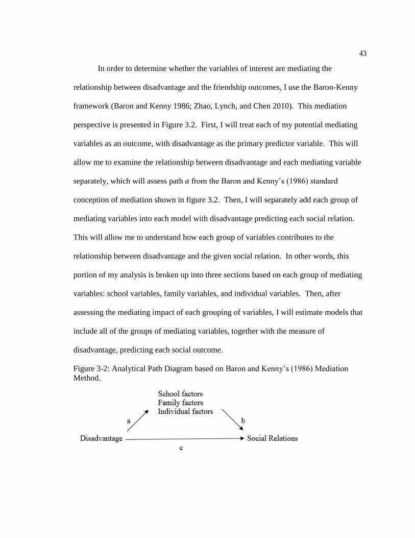
43

In order to determine whether the variables of interest are mediating the

relationship between disadvantage and the friendship outcomes, I use the Baron-Kenny

framework (Baron and Kenny 1986; Zhao, Lynch, and Chen 2010). This mediation

perspective is presented in Figure 3.2. First, I will treat each of my potential mediating

variables as an outcome, with disadvantage as the primary predictor variable. This will

allow me to examine the relationship between disadvantage and each mediating variable

separately, which will assess path a from the Baron and Kenny’s (1986) standard

conception of mediation shown in figure 3.2. Then, I will separately add each group of

mediating variables into each model with disadvantage predicting each social relation.

This will allow me to understand how each group of variables contributes to the

relationship between disadvantage and the given social relation. In other words, this

portion of my analysis is broken up into three sections based on each group of mediating

variables: school variables, family variables, and individual variables. Then, after

assessing the mediating impact of each grouping of variables, I will estimate models that

include all of the groups of mediating variables, together with the measure of

disadvantage, predicting each social outcome.

Figure 3-2: Analytical Path Diagram based on Baron and Kenny’s (1986) Mediation

Method.

44

Additionally, to test the statistical significance and specific effects of each

mediating variable, I will calculate the indirect effects and percentage-mediated of each

of the mediating variables. The indirect effects of each mediating variable is calculated

by multiplying paths a (mediator regressed on disadvantage) and b (social relation

regressed on mediator) of the mediation model. Then, I will use the RMediation software

to obtain the 95% confidence interval of each indirect effect. To determine the

percentage of mediation, I will use (ab / (∑ab+c’))*100, where ∑ab = the sum of the

indirect effects and c’ is the path from disadvantage to the social relation from each

model that includes the grouped mediating variables (Rulison, Feinberg, Gest, and

Osgood 2015; MacKinnon 2012; Tofighi and MacKinnon 2011). The percentage

explained by each of the mediating variables is presented in a second table in each

section of the results, with asterisks to indicate significance values.

Results

Bivariate Analyses

Table 3.2 and Figure 3.3 present the results from t-tests to determine a base

relationship between disadvantage and the four friendship outcomes. The table presents

results when using all eight waves of data, while the figure presents the results wave-by-

wave. The empirical Bayes FRL continuous variable was recoded into a binary variable

45

for this bivariate analysis, with those adolescents scoring in the top 15%4 of the empirical

Bayes FRL variable being coded as disadvantaged, and everyone else being coded as

non-disadvantaged. Disadvantage significantly and negatively affects all four of the

friendship outcomes. Disadvantaged students, on average, receive about one fewer

friendship nomination, score approximately 30% lower in Bonacich centrality, have

lower reciprocity rates, and lower friendship stability rates as compared to non-

disadvantaged students. I also included a column in Table 3.2 with the differences in

standard deviation units (Cohen’s d) for each of the effect sizes to determine which of the

social measures disadvantage has the strongest/weakest effect upon. It is evident that

disadvantage has a stronger effect upon in-degree and Bonacich centrality as compared to

reciprocity and stability. It is also noteworthy that the relationship between disadvantage

and the friendship outcomes is relatively stable from sixth through twelfth grade. Though

most of the measures do begin to converge in eleventh and twelfth grade, this may arise

because students are able to begin dropping out of high school beginning at age 16

(approximately between waves 6 and 7).

Dropout might contribute to the convergence in these measures because it seems

likely that disadvantaged students scoring the lowest on these friendship outcomes are

arguably the most likely to drop out of school (Rumberger and Larson 1998; Wehlage et

al. 1989). To test whether differential dropout might account for this convergence, I

completed some additional tests. Since disadvantage is negatively associated with the

social measures (Table 3.2), it seems likely that the most disadvantaged adolescents are

4 The top 15% was chosen as the cut-off because communities must have had at least 15% of the

students receiving FRL to be selected as a part of the PROSPER sample. Thus, I use this percentage as the

cut-off to determine who is selected as “disadvantaged” for the bivariate analyses.

46

the least likely to be popular and have stable/reciprocated friendships. Therefore, if the

most disadvantaged of the adolescents begin to leave the sample, then there should be

some convergence in the social measures. Based on this, I completed an additional check

on whether this is a likely explanation for these results. In general, there is some attrition

in the PROSPER sample as the adolescents age, especially in the later waves of the study.

Tracking the average disadvantage of the sample from wave-to-wave indicates whether

the students leaving the sample are more or less disadvantaged than average. The

empirical Bayes FRL measure of disadvantage is constant for each individual across all

waves of the sample. Therefore, the average score of disadvantage for the sample should

remain relatively constant over time if the sample remains similar across all eight waves

of data, or if leaving the sample is not correlated with disadvantage. If disadvantaged

adolescents disproportionately leave the sample, then the mean of disadvantage for the

sample should decrease.

The average of disadvantage remains relatively stable from waves 1 to 5,

fluctuating between -0.12 and -0.15, indicating little change in the sample, or at least that

any sample change is not correlated with disadvantage. However, disadvantage begins to

sharply decline in wave 6, dropping to -0.21, then -0.25 in wave 7, to -0.30 in wave 8. In

other words, leaving the sample in the later waves of the study is correlated with

disadvantage. Thus, it seems likely that the convergence evident in waves 6 through 8 is

because of the most disadvantaged adolescents dropping out of school.

Table 3-2: Comparison of Means Tests for In-Degree, Bonacich Centrality, Reciprocity

and Friendship Stability by Disadvantage, combining all eight waves of data.

47

Disad. Non-Dis Total Cohen’s d

In-Degree 2.49 3.49 3.35 0.38

Bonacich Cent. 0.53 0.81 0.77 0.48

Reciprocity Rate 0.46 0.51 0.50 0.17

Stability Rate 0.37 0.42 0.41 0.17

Notes: T-Tests combined all 8 waves of data for in-degree, Bonacich, and

reciprocity. For stability, these results combined waves 2 through 8. All results

statistically significant at p<0.001 level. "Disadvantage" binary variable consists

of top 15% of continuous variable coded as disadvantage, remainder of sample

coded as non-disadvantage.

Figure 3-3: Comparison of Means Tests for In-Degree, Bonacich Centrality, Reciprocity,

and Friendship Stability by Disadvantage.

1.00

2.00

3.00

4.00

5.00

Wave1

Wave2

Wave3

Wave4

Wave5

Wave6

Wave7

Wave8

In-Degree

Disad Non-Dis

0.40

0.50

0.60

0.70

0.80

0.90

1.00

Wave1

Wave2

Wave3

Wave4

Wave5

Wave6

Wave7

Wave8

Bonacich Centrality

Disad Non-Dis

0.30

0.40

0.50

0.60

Wave1

Wave2

Wave3

Wave4

Wave5

Wave6

Wave7

Wave8

Reciprocity Rate

Disad Non-Dis

0.20

0.30

0.40

0.50

0.60

Wave1

Wave2

Wave3

Wave4

Wave5

Wave6

Wave7

Wave8

Stability Rate

Disad Non-Dis

48

Multi-level Results

Disadvantage and Social Relations

Table 3.3 presents the results from multilevel models in which disadvantage is

predicting the four separate social relations when controlling for sex, race, treatment

condition, and wave. Model I is an overdispersed Poisson multilevel model predicting

In-Degree. Bonacich centrality is the outcome in Model II, which is a normal HLM

equation. Models IIII and IV are both binomial models that predict reciprocity and

stability, respectively. Disadvantage has a significant and negative relationship with each

of the four outcomes. To reiterate, the measure of disadvantage was created using

empirical Bayes shrinkage estimates in HLM, aggregating together each student’s

responses to a question assessing whether or not that student received free/reduced-priced

lunch, with higher scores indicating disadvantage. Disadvantage reduces the likelihood

of receiving friendship nominations. This net effect is equivalent to approximately a 17%

decrease in the number of friendship nominations when comparing students who differ in

disadvantage by one standard deviation. Adolescents that are more disadvantaged also

tend to score lower in Bonacich centrality as compared to their peers. For each sent

nomination, increases in disadvantage decreases the odds of receiving a reciprocated

friendship nomination. For each received friendship nomination at T1, the odds of

maintaining that friendship to T2 decreases as disadvantage increases. All of these results

indicate that the relationship between disadvantage and the four social relations should be

explored further to determine what factors are mediating these relationships.

[Table 3.3 about here]

49

Relationship between Disadvantage and Mediators

The next section of analysis assesses the relationship of disadvantage to each of

the potential mediators. This is path a of the Baron-Kenny mediation model, and is one

of the two relationships that must come together to create mediation: the stronger this

relationship, the greater the potential for that variable to mediate its impact on the

outcome. Each of my mediating variables was regressed on disadvantage in a 3-level,

multilevel model while controlling for sex, race, wave, and treatment condition.

Presented in Table 3.4, these results demonstrate that disadvantage is a

statistically significant predictor of all of the mediating variables, with the exception of

parental communication. Disadvantage is most-strongly related to student grades and

family home condition, giving them special potential to mediate its relationships with the

outcomes of interest. Each one-unit increase in disadvantage results in an expected

decrease of 0.142 in grades, while controlling for sex, race, wave, and treatment

condition. The condition of the family home (i.e., the cleanliness, organization, upkeep)

is expected to decrease as the disadvantage of the adolescent increases. Additionally,

disadvantage is a moderately-strong predictor of getting into trouble at school, unexcused

absences, parental school involvement, poor mental health, poor physical health, and

attractiveness.

[Table 3.4: Disadvantage Predicting Mediating Variables, about here]

50

School Variables as Mediators

Table 3.5 presents the results when including the school measures in the analysis

as mediating variables. Each Model treats a different social relation as an outcome, and

controls for sex, race, wave, and treatment condition. Also, the coefficient for

disadvantage from the previous set of analyses is included as an easy-reference to

approximate the amount of mediation that is occurring. In other words, the previous set

of analyses that included only disadvantage (and the control variables) predicting in-

degree demonstrated that each one-unit increase in disadvantage results in approximately

a 10% decrease in the number of friendship nominations received, which is included at

the top of Table 3.5. Additionally, Table 3.6 presents the mediation results in terms of

the percentage of the total relationship of disadvantage to the outcome that each school

variable mediates, or accounts for. To reiterate, the percentage of mediation is calculated

by computing the indirect effects of each mediating variable and using (ab /

(∑ab+c’))*100. Then, RMediation was used to obtain the 95% confidence interval of

each indirect effect. The significance of each effect is indicated with asterisks in the

table.

[Table 3.5: 3-Level, Multilevel Models of Disadvantage Predicting In-Degree, Bonacich,

Reciprocity, and Stability with the School Mediating Variables, about here]

[Table 3.6: Percentage of Mediation explained by School Variables, about here]

After including the school variables, disadvantage remains a negative predictor of

in-degree, Bonacich centrality, reciprocity, and stability. Student grades is a statistically

significant predictor of in-degree, Bonacich centrality, and friendship stability, though it

appears to be more strongly related to in-degree and Bonacich centrality. Educational

51

aspirations is also significantly related to popularity, with each one-unit increase in

educational aspirations resulting in a 0.036 increase in Bonacich centrality. Getting into

trouble at school is significantly related to the qualitative elements of friendships

(reciprocity and stability), but not to the measures more indicative of popularity (in-

degree and Bonacich centrality). Interestingly, the relationship between school bonding

and reciprocity is negative, and this is the only model when school bonding is a

statistically significant predictor. Each one-unit increase is the measure of school

bonding results in almost a 10% decrease in the odds of receiving a reciprocal friendship

nomination, when controlling for the other variables in the model. Keeping in mind that

this is a binomial model that accounts for the number of sent friendship nominations, this

is a surprising finding. It could be that as students feel more bonded to school, it results

in less time to spend balancing friendships.

The school measures mediate the relationship between disadvantage and in-

degree by about 13%. When Bonacich centrality is the outcome, the coefficient for

disadvantage changes from -0.077 to -0.064 with the inclusion of the school variables,

approximately a 17% change. The relationship between disadvantage and reciprocity is

mediated by approximately 13% by the school variables. The biggest change occurs

when predicting friendship stability, with the school attributes mediating approximately

40% of the effect of disadvantage. However, this is most likely in part because

disadvantage is less related to stability than the other three outcomes. This means that

this is a bigger percentage of a smaller relationship, so it is really not a very different

effect size.

52

Student grades is the most influential, and the only statistically significant,

mediator from the school attributes, accounting for between 9 and 22% of the relationship

between disadvantage and the four social relations. This makes sense based on the

previous analysis that demonstrated the strong relationship between disadvantage and

student grades (path a), making grades especially likely to be a significant mediator.

Though the mediating effect of grades is relatively consistent in the models predicting in-

degree, Bonacich centrality, and reciprocity (9%, 13%, and 12%, respectively), grades

has the strongest mediating impact on friendship stability (22.78%). However, as

mentioned above, this should be considered relative to the results that demonstrated that

disadvantage is less related to stability than the other three outcomes. None of the

remaining variables were as consistently associated with the measures of peer relations.

Educational aspirations account for almost 3% of the relationship with in-degree and

Bonacich centrality, but then has a suppressor effect when predicting reciprocity and

stability. Conversely, getting into trouble does not seem to have a mediating impact

when predicting in-degree and Bonacich centrality, but accounts for 5 and 10% mediation

when predicting reciprocity and stability. However, none of the other measures are

significant mediators of the relationship between disadvantage and the four social

relations.

In sum, the school attributes partially mediated the relationship between

disadvantage and each of the four social relations. The relationship between in-degree

and Bonacich centrality was mediated by approximately 13% and 17%, respectively.

Upon calculating the indirect effects and p-values for each of the mediating variables,

only student grades is a statistically significant mediator of the relationship between

53

disadvantage and the four social relations. Additionally, school grades is the strongest

predictor of in-degree and Bonacich centrality within the school attributes. When

treating the qualitative elements of friendships as outcomes, getting into trouble at school

has the strongest relationship with friendship reciprocity and stability of the school

attributes.

Family Variables as Mediators

Next, I replace the school variables with the family mediating variables.

Presented in Table 3.7, each model treats one of the four social relations as an outcome

and each model is a 3-level, multilevel model that controls for sex, race, wave, and

treatment condition. Also, as before, the coefficient for disadvantage from the first set of

analyses is included at the top of the table to reference. Additionally, Table 3.8 presents

the percentage of mediation explained by each of the variables, along with asterisks to

indicate which of the indirect effects are statistically significant.

[Table 3.7: 3-Level, Multilevel Models of Disadvantage Predicting In-Degree, Bonacich,

Reciprocity, and Stability with the Family Mediating Variables, about here]

[Table 3.8: Percentage of Mediation explained by Family Variables, about here]

Disadvantage remains a significant predictor of in-degree, Bonacich centrality,

and reciprocity. However, after the inclusion of the family variables, disadvantage is no

longer a significant predictor of stability. Family home condition has a significant effect

on all four of the social relations. Parental communication also has a relatively strong

effect on both in-degree and Bonacich centrality, though previous analyses made it

54

known that this is not a mediator of disadvantage. Additionally, family relations is a

significant predictor of friendship stability, with each one-unit increase in family relations

increasing the odds of having a stable friendship from T1 to T2 by about 18%.

Overall, the relationship between disadvantage and each of the four social

relations is partially mediated by the family variables, with the largest mediation

occurring, once again, when friendship stability is the outcome. Family home condition

is the only variable of the family measures to have a statistically significant mediating

impact on the relationship between disadvantage and all four of the social relations. To

reiterate, family home condition is an interviewer-reported scale, with a range of 1 to 5,

which is based on the cleanliness, upkeep, and organization of the home. Family home

condition accounts for 21% of the relationship between disadvantage and in-degree, 17%

of relationship between disadvantage and Bonacich centrality, 32% of relationship

between disadvantage and reciprocity, and almost 49% of relationship between

disadvantage and friendship stability. Additionally, parental school involvement is a

significant mediator of the relationship between disadvantage and in-degree, and

disadvantage and Bonacich centrality, accounting for approximately 3% mediation of

each relationship. Also, family relations significantly accounts for almost 7% of the

relationship between disadvantage and friendship stability.

In sum, the family variables partially mediated the relationship between

disadvantage and each of the four social relations, and seemed to have a slightly larger

mediating-impact than the school variables. Family home condition stood out from the

other family attributes by having a significant relationship with each of the four social

relations. Parental school involvement is a significant mediator of the relationship

55

between disadvantage and both in-degree (2.45%) and Bonacich centrality (3%). Family

relations is a significant mediator of the relationship between disadvantage and friendship

stability, accounting for over 6%. Parental school involvement has a significant and

positive relationship with both in-degree and Bonacich centrality, though not with

reciprocity and stability. Family relations is a significant predictor of friendship stability,

but is not significantly related with any of the other social relations.

Other Individual Variables as Mediators

Next, I replaced the family variables with the other individual mediating

variables. To reiterate, the individual variables assess traits and characteristics of the

respondent, and include measures of mental health, physical health, attractiveness,

bullying, and nervousness. Table 3.9 presents the results of the 3-level, multilevel

models that include the individual mediating variables with disadvantage as the primary

predictor, while controlling for sex, race, wave, and treatment condition. Additionally, at

the top of the table I include the coefficients for disadvantage from the original analysis

as a reference for mediation. Table 3.10 presents the percentages of mediation that each

individual measure accounts for, with asterisks to indicate statistical significance.

[Table 3.9: 3-Level, Multilevel Models of Disadvantage Predicting In-Degree, Bonacich,

Reciprocity, and Stability with the Individual Mediating Variables, about here]

[Table 3.10: Percentage of Mediation explained by Individual Variables, about here]

All of the individual measures, except for bullying, have a significant relationship

with in-degree. Each one-unit increase in the scale assessing poor mental health

56

decreases friendship nominations by about 14%. The next strongest predictor of in-

degree is nervousness, with each one-unit increase in nervousness decreasing friendship

nominations by about 7%. Attractiveness, which was interviewer-reported at each in-

home interview, is significantly and positively related to in-degree. Each one-unit

increase in attractiveness increases receiving friendship nominations by approximately

5%. Poor physical health is significantly and negatively related to in-degree.

Poor mental health, poor physical health, and attractiveness are all significantly

related to Bonacich centrality. Each one-unit increase in the scale measuring poor mental

health results in a 0.084 decrease in Bonacich centrality. Poor physical health is

inversely related to Bonacich centrality, in that each one-unit increase in poor physical

health decreases Bonacich centrality by 0.045. And, similar to in-degree, attractiveness is

positively related to Bonacich centrality. Unlike in-degree, however, bullying is

significantly related to Bonacich centrality while nervousness is not. Each one-unit

increase in the measure of bullying results in an expected decrease of 0.043 in Bonacich

centrality.

Poor mental health is the strongest predictor of both friendship reciprocity and

friendship stability. Additionally, poor physical health is inversely related to friendship

stability. Each one-unit increase in poor physical health decreases the odds of a

friendship from T1 repeating in T2 by almost 6%. Interestingly, none of the other

individual variables are significantly related to either reciprocity or stability.

The individual variables partially mediate the relationship between disadvantage

and each of the four social relations, with varying magnitude. When examining Model I,

the coefficient for disadvantage decreases in magnitude from -0.105 to -0.085 (almost a

57

20% change) with the inclusion of the individual measures. The inclusion of the

individual variables mediates the relationship between disadvantage and Bonacich

centrality by approximately 15%. Meanwhile, the relationship between disadvantage and

reciprocity is mediated by 16% from the inclusion of the individual variables (Model III).

Finally, the largest percentage change occurs in with friendship stability as the outcome,

but this is also where disadvantage has the weakest relationship.

For each of the models, poor mental health has the strongest mediating impact.

Poor mental health accounts for between 7% and almost 25% of the relationship between

disadvantage and the four social relations: 10% for in-degree, 7% for Bonacich centrality,

14% for reciprocity, and 25% for stability. Poor physical health is a significant mediator

in the models predicting in-degree, Bonacich centrality, and stability accounting for

approximately 2%, 3%, and 6% of each relationship, respectively. Attractiveness is a

significant mediator in the models predicting in-degree and Bonacich centrality,

accounting for almost 3% of those relationships

In sum, the individual variables partially mediate the relationship between

disadvantage and each of the four social relations. The strongest mediator of the

individual variables in all four models is poor mental health, accounting for between 7

and 25% mediation between the outcomes. Poor physical health is a significant mediator

when in-degree, Bonacich centrality, and stability are the outcomes. Also, attractiveness

is a significant mediator when predicting in-degree and Bonacich centrality. Poor

physical health is also an important predictor of all four social relations, except for

reciprocity. Additionally, attractiveness is positively related to both in-degree and

58

Bonacich centrality. Finally, nervousness is negatively related to in-degree, while

bullying is negatively related to Bonacich centrality.

Inclusion of all Mediating Variables

The next stage of analysis includes all three groups of mediating variables in the

models. Again, each model is a 3-level, multilevel model that controls for sex, race,

wave, and treatment condition. These results are presented in Table 3.11. For the

purposes of space, I did not include the results for the control variables in the table. The

percentage of mediation that each measure accounts for is included in Table 3.12.

[Table 3.11: 3-Level, Multilevel Models of Disadvantage Predicting In-Degree,

Bonacich, Reciprocity, and Stability with All Mediating Variables, about here]

[Table 3.12: Percentage of Mediation explained by All Mediating Variables, about here]

In the final models, disadvantage remains a negative predictor of in-degree and

Bonacich centrality, but is no longer significantly related to reciprocity or stability.

Grades, family home condition, poor mental health, poor physical health, and

nervousness are all significantly related to in-degree in the full analysis. Similarly,

grades, family home condition, poor mental health, and poor physical health are all

significant predictors of Bonacich centrality. However, getting into trouble at school,

educational aspirations, parental school involvement, and attractiveness are also all

significant predictors of Bonacich centrality in the full analysis. Interestingly, school

bonding is still negatively related to friendship reciprocity. Family home condition and

59

poor mental health remain significantly related to friendship reciprocity, as well. Grades

and family home condition are both significantly related to friendship stability.

The relationships between disadvantage and in-degree, Bonacich centrality, and

reciprocity were all mediated by just over 40% (41.8%, 40.6%, and 43.1%, respectively).

Meanwhile, the greatest percentage mediation occurred in Model IV, where the

relationship between disadvantage and friendship stability was almost completely

mediated (92.5%). With the inclusion of all of the mediating variables, each one-unit

increase in disadvantage decreases the odds of receiving a friendship nomination by

about 6%, decreases Bonacich centrality by about 0.046 (about 1.5%), the odds of

receiving a reciprocal friendship nomination by about 5%, and maintaining a friendship

from T1 to T2 by about a 0.5%. Interestingly, it is evident that no one group (i.e., school,

family, individual) of mediating variables can take all of the credit for the partial

mediation in the final models. Rather, specific variables from each of the groups had the

most impact on mediating the relationship between disadvantage and the four social

relations.

School grades is a significant mediator of the relationship between disadvantage

and in-degree (8%), Bonacich centrality (10%), and friendship stability (24%). None of

the other indirect effects of the school attributes were statistically significant. The

condition of the family home is always the strongest mediator in each of the four models,

accounting for almost 19% mediation of the relationship between disadvantage and in-

degree, 14% when predicting Bonacich centrality, 28% in when predicting reciprocity,

and approximately 42% when predicting stability. Parental school involvement is a

significant mediator of the relationship between disadvantage and Bonacich centrality,

60

accounting for almost 3%. Poor mental health accounted for approximately 9% of the

relationship between disadvantage and in-degree, and almost 7% of the relationship

between disadvantage and Bonacich centrality. Poor physical health accounted for just

over 3% mediation when predicting in-degree and Bonacich centrality. Attractiveness

accounted for almost 3% of the relationship between disadvantage and Bonacich

centrality, but was not a significant mediator in any of the other final models. Though

grades and mental health accounted for a moderate amount of mediation when predicting

reciprocity, neither of these effects were statistically significant. This may be because

that, while these variables are explaining a moderate percentage of the relationship, the

relationship between disadvantage and reciprocity is weaker than that of in-degree and

Bonacich centrality. Thus, these variables are explaining a large percent of a smaller

relationship.

In sum, the relationships between disadvantage and in-degree, Bonacich

centrality, and reciprocity were each mediated by just over 40% with the inclusion of all

of the mediating variables. Meanwhile, the relationship between disadvantage and

friendship stability was almost completed mediated (92.5%). Family home condition is

the strongest mediator in each of the models. Grades is a significant mediator of the

relationships between disadvantage and in-degree, Bonacich centrality, and stability.

Poor mental health accounts for 9% and 6% when predicting in-degree and Bonacich

centrality, respectively. Poor physical health is also a significant mediator when

predicting in-degree and Bonacich centrality, accounting for just over 3% mediation in

each model. Parental school involvement and attractiveness are significant mediators of

61

the relationship between disadvantage and Bonacich centrality, with each variable

accounting for almost 3% mediation of the relationship.

Sensitivity Analyses

As discussed in Chapter 1, there is a chance that the bounds of the available social

network data (i.e., being limited to in-grade and in-school friendships) may be

influencing the given study. To help alleviate this concern, I completed additional

analyses that examined out-of-school and out-of-grade friends. Beginning in wave 4,

respondents were asked to report the number of out-of-school friends they have, as well

as the number of out-of-grade friends they have. I conducted comparison of means tests

examining the relationship between disadvantage and the number of friends one has in

other schools and in other grades. On average, when aggregating waves four through

eight, there is not a statistically significant relationship between disadvantage and having

friends in other grades. Disadvantaged adolescents have, on average, 5.65 friends in

other grades, while non-disadvantaged adolescents have, on average, 5.62 friends in other

grades (t = -0.745, p = 0.456). When examining the number of friends in other schools,

disadvantaged adolescents have a higher amount, on average, of out-of-school friends

than non-disadvantaged adolescents, but the difference is rather small (4.97 compared to

4.72; t=-4.549, p = 0.000).

Additionally, I re-estimated some of the primary analyses of this chapter that

included the out-of-grade and out-of-school friends as control variables. More

specifically, I re-estimated the full models predicting Bonacich centrality, friendship

62

reciprocity, and friendship stability. In general, none of my primary results were

impacted when including these measures as control variables. For example, when re-

estimating my full model that predicted Bonacich centrality, the significance values of all

of the school, family, and individual variables did not change. School grades, getting into

trouble, educational aspirations, family home condition, parental school involvement,

poor mental health, poor physical health, and attractiveness are all still significant

predictors of Bonacich centrality, and none of the other variables in the model are

significant. Further, the measures for out-of-grade friends (coef. = 0.007, se = 0.005) and

out-of-school friends (coef. = -0.006, se = 0.006) are not statistically significant in this

model. Additionally, the measures for out-of-grade friends and out-of-school friends

were not significant mediators in any of these supplemental analyses. Taken together,

these bivariate and multivariate supplemental analyses indicate that out-of-school

friendships and/or out-of-grade friendships are not significantly impacting this chapter of

my dissertation. In other words, these analyses alleviate concerns of the in-school, in-

grade network bounding of the dataset.

Supplemental Analyses

I also estimated multilevel models separately predicting the four social measures

using other forms of disadvantage as the primary predictor variables. These results are

presented in Tables 3.13-3.16. For these supplemental analyses, each model included a

different measure for disadvantage, either household income, parental education, whether

or not the respondent lives with both biological parents, or a composite SES variable.

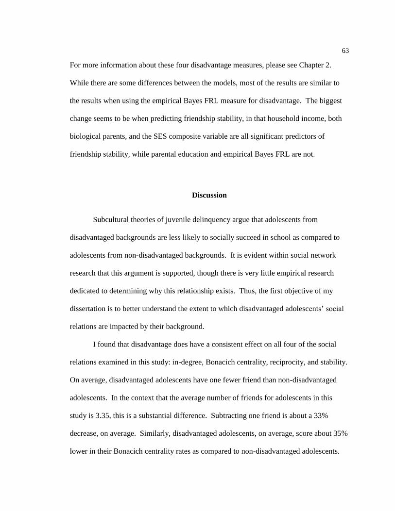
63

For more information about these four disadvantage measures, please see Chapter 2.

While there are some differences between the models, most of the results are similar to

the results when using the empirical Bayes FRL measure for disadvantage. The biggest

change seems to be when predicting friendship stability, in that household income, both

biological parents, and the SES composite variable are all significant predictors of

friendship stability, while parental education and empirical Bayes FRL are not.

Discussion

Subcultural theories of juvenile delinquency argue that adolescents from

disadvantaged backgrounds are less likely to socially succeed in school as compared to

adolescents from non-disadvantaged backgrounds. It is evident within social network

research that this argument is supported, though there is very little empirical research

dedicated to determining why this relationship exists. Thus, the first objective of my

dissertation is to better understand the extent to which disadvantaged adolescents’ social

relations are impacted by their background.

I found that disadvantage does have a consistent effect on all four of the social

relations examined in this study: in-degree, Bonacich centrality, reciprocity, and stability.

On average, disadvantaged adolescents have one fewer friend than non-disadvantaged

adolescents. In the context that the average number of friends for adolescents in this

study is 3.35, this is a substantial difference. Subtracting one friend is about a 33%

decrease, on average. Similarly, disadvantaged adolescents, on average, score about 35%

lower in their Bonacich centrality rates as compared to non-disadvantaged adolescents.

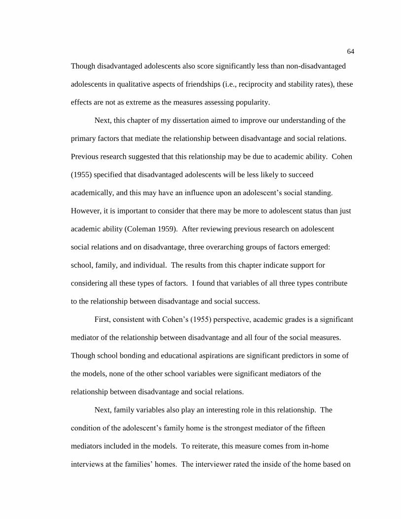
64

Though disadvantaged adolescents also score significantly less than non-disadvantaged

adolescents in qualitative aspects of friendships (i.e., reciprocity and stability rates), these

effects are not as extreme as the measures assessing popularity.

Next, this chapter of my dissertation aimed to improve our understanding of the

primary factors that mediate the relationship between disadvantage and social relations.

Previous research suggested that this relationship may be due to academic ability. Cohen

(1955) specified that disadvantaged adolescents will be less likely to succeed

academically, and this may have an influence upon an adolescent’s social standing.

However, it is important to consider that there may be more to adolescent status than just

academic ability (Coleman 1959). After reviewing previous research on adolescent

social relations and on disadvantage, three overarching groups of factors emerged:

school, family, and individual. The results from this chapter indicate support for

considering all these types of factors. I found that variables of all three types contribute

to the relationship between disadvantage and social success.

First, consistent with Cohen’s (1955) perspective, academic grades is a significant

mediator of the relationship between disadvantage and all four of the social measures.

Though school bonding and educational aspirations are significant predictors in some of

the models, none of the other school variables were significant mediators of the

relationship between disadvantage and social relations.

Next, family variables also play an interesting role in this relationship. The

condition of the adolescent’s family home is the strongest mediator of the fifteen

mediators included in the models. To reiterate, this measure comes from in-home

interviews at the families’ homes. The interviewer rated the inside of the home based on

65

cleanliness, organization, and maintenance. The effect of this variable on social relations

could be operating through one of several mechanisms.

First, as discussed previously, parents influence friendship formation by

monitoring the type of peer-interactions that they have (Crosnoe 2000; Parke and

Bhaynagri 1989). Thus, if parents are dropping their child off at a friend’s house and

notice that the house is not very-well maintained or is not very clean, then the parents

may restrict their child from going back over to that house. I would argue that this is the

essence of this measure because it arises from an adult (the interviewer) visiting a home

for the first time and making snap judgements regarding the cleanliness, organization,

and upkeep of the home.

Second, the impact of family home condition on social relations may be because

of the judgment of one’s peers. As discussed previously, adolescents, even as young as

sixth grade, are able to make judgments on the characteristics of the family home (Cohen

1955). Children may be self-selecting not to go over a friend’s house if it is unclean or

disorganized. A third mechanism that the condition of the family home may operate

through is from the viewpoint of the child living in the home. In other words, if a child

recognizes that his/her own house is disorganized, ill maintained, and/or unclean,

especially in comparison to other children’s homes, then the child may be hesitant to

invite other children over out of embarrassment. This may cause a detrimental effect on

one’s ability to make friends because of a lack of initiation and/or reciprocation.

Finally, this finding may be related to research that focuses on chaotic

environments and the impact that this may have on psychological and social outcomes.

“Applied to the social and psychological reality of family life, chaos refers to high levels

66

of confusion and agitation in the home, as well as to a sense of rush, disorganization, and

pressure of time in daily routines” (Dumas et al. 2005:93). Home chaos has been linked

to numerous negative outcomes for both adults and children living in the home, such as

parenting difficulties, child behavior problems, and cognitive development (Petrill et al.

2004; Johnson et al. 2008; Bradley 2004). Further, Dumas and colleagues (2005:101)

demonstrated that, though the CHAOS construct is correlated with measures such as

socioeconomic status and neighborhood attributes, home chaos is not a proxy but is a

useful construct in its own right. Though my measure of family home condition is not

nearly as comprehensive as the CHAOS scale used in this area of research, it appears to

capture similar themes, and which may account for the similar results. Future research

may be able to further explain the nature of this mechanism.

Two other family variables have a significant mediating impact on the

relationship between disadvantage and social relations. First, the family relations

composite measure is a significant mediator between disadvantage and stability of one’s

friendships. Again, the mechanism(s) that this operates through is unclear, but it is

interesting that this variable only affects the stability of friendships, but not the other

three social relations. It may be that, when children have poor relationships in the many

ways captured by this measure, then other children do not want to continue spending time

in that less than pleasant environment. Conversely, this could also be because the child

may not be learning specific social skills from his/her relationships with his/her parents

that would be valuable for maintaining friendships. Much of the family relations measure

is based on spending quality time with one’s parents (i.e., engaging in activities that both

the child and parents enjoy; do something active together; talk about future plans; express

67

appreciation towards one another). If the child does not actively engage in these types of

activities with one’s parents, then maybe the child is not learning how to effectively

engage in some of these activities with friends, thus limiting one’s ability to maintain

friendships. This is an interesting relationship that deserves additional attention in future

research.

Next, parental school involvement plays a small mediating role in the relationship

between disadvantage and popularity (i.e., in-degree and Bonacich centrality). As

discussed previously, this may be because such parental involvement brings an increase

in parental social capital that can in turn increase opportunities for adolescents to

socialize. In other words, parents actively involved in school functions will get to know

one another and, potentially, befriend one another, thus increasing the opportunities that

their children will get to know one another. However, parents of a lower socioeconomic

status are less likely to be involved in school-related activities than parents of a higher

socioeconomic status (Hill and Taylor 2004), which may limit children from a

disadvantaged background’s access to this avenue of friendship formation.

Finally, my results indicated that specific individual characteristics also play a

mediating role in the relationship between disadvantage and social relations. As

discussed in the background chapter of this dissertation, previous research has

demonstrated that health in adolescence is associated with one’s social class (Starfield,

Riley, Witt, and Robertson 2002) and that health can have important ramifications for

social relations (Bronfenbrenner and Morris 2006; Simpkins, Schaefer, Price, and Vest

2013). Results in this chapter demonstrate that poor mental health and poor physical

health are significant mediators of the relationship between disadvantage and the two

68

popularity measures, but not of the two qualitative measures. A similar effect is also

evident with attractiveness. Attractiveness is a significant mediator of the relationship

between disadvantage and popularity, but not of disadvantage and qualitative aspects of

friendships.

In sum, I found that disadvantage does have a consistent effect on all four of the

social relations examined in this study: in-degree, Bonacich centrality, reciprocity, and

stability. Additionally, this chapter of my dissertation improved our understanding of the

primary factors that mediate the relationship between disadvantage and social relations,

demonstrating support that all three (i.e., school, family, and individual) types of factors

should be considered.

69

Table 3-3: 3-Level, Multilevel Models of Disadvantage Predicting In-Degree, Bonacich, Reciprocity, and Stability.

Model I: In-Degree Model II: Bonacich Model III: Reciprocity Model IV: Stability

R.R. Coef. RSE Coef. RSE O.R. Coef. RSE O.R. Coef. RSE

Disadvantage

Emp. Bayes FRL 0.900 -0.105 0.012 *** -0.077 0.009 *** 0.919 -0.084 0.022 *** 0.946 -0.056 0.015 ***

Controls

Intercept 3.478 1.246 0.070 *** 0.861 0.054 *** 1.533 0.427 0.097 *** 0.955 -0.046 0.097

Male 0.805 -0.216 0.027 *** -0.161 0.031 *** 0.828 -0.189 0.052 ** 0.963 -0.038 0.050

White 0.971 -0.029 0.062

-0.010 0.049

1.070 0.068 0.086

1.257 0.229 0.071 **

Treatment 0.962 -0.038 0.049

-0.008 0.031

0.924 -0.079 0.074

1.071 0.068 0.089

Wave 2 1.189 0.173 0.043 *** 0.053 0.022 * 0.912 -0.092 0.057

-- -- --

Wave 3 1.207 0.188 0.059 ** 0.035 0.032

0.953 -0.048 0.080

0.508 -0.678 0.078 ***

Wave 4 1.165 0.153 0.060 * 0.049 0.034

0.950 -0.052 0.090

0.586 -0.053 0.061 ***

Wave 5 0.993 -0.007 0.056

0.033 0.031

0.876 -0.133 0.098

0.553 -0.593 0.056 ***

Var. Comp. VC SD VC SD VC SD VC SD

Level 3

0.006 0.077 * 0.001 0.028

0.015 0.123 **

0.034 0.186 ***

Level 2

0.278 0.527 *** 0.154 0.392 ***

0.244 0.494 ***

0.195 0.442 ***

Level 1 0.919 0.959 0.135 0.368 -- -- -- --

Notes: Level 1 N=3500; Level 2 N= 908, Level 3 N=27. *p<0.05, **p<0.01, ***p<0.001. Abbreviations: R.R. = Risk Ratio, RSE = Robust Standard

Error, O.R. = Odds Ratio, Emp. = Empirical, VC = Variance Component, and SD = Standard Deviation. Wave 1 is the reference variable in Models I-III.

Wave 2 is the reference variable in Model IV. Female is the reference variable to male. Non-white is the reference variable to white.

70

Table 3-4: Disadvantage Predicting Mediating Variables.

Predictor Mediator as Outcome Coef. RSE

Disadvantage School Measures

Grades -0.142 0.012 ***

School Bonding -0.046 0.014 **

Getting into Trouble 0.054 0.014 ***

Educ. Aspirations -0.055 0.010 ***

Absences 0.082 0.018 ***

Family Measures

Family Relations -0.024 0.007 **

Family Home Condition -0.262 0.019 ***

Family Location 0.044 0.009 ***

Parental Comm. -0.008 0.007

Parental Sch. Involv. -0.061 0.018 **

Individual Measures

Poor Mental Health 0.072 0.010 ***

Poor Physical Health 0.059 0.015 ***

Attractiveness -0.059 0.008 ***

Bullies Others 0.035 0.007 ***

Nervous 0.022 0.007 **

Notes: Level 1 N=3500; Level 2 N= 908, Level 3 N=27. *p<0.05, **p<0.01,

***p<0.001. Abbreviations: Coef. = Coefficient; RSE = Robust Standard Error. All

models controlled for sex, race, wave, and treatment condition.

71

Table 3-5: 3-Level, Multilevel Models of Disadvantage Predicting In-Degree, Bonacich, Reciprocity, and Stability with the

School Variables.

Model I: In-Degree Model II: Bonacich Model III: Reciprocity Model IV: Stability

R.R. Coef. RSE Coef. RSE O.R. Coef. RSE O.R. Coef. RSE

Disadvantage

Empirical Bayes FRL 0.900 -0.105 0.012 *** -0.077 0.009 *** 0.919 -0.084 0.022 *** 0.946 -0.056 0.015 ***

Empirical Bayes FRL 0.913 -0.091 0.013 *** -0.064 0.009 *** 0.930 -0.073 0.021 ** 0.967 -0.033 0.014 *

School Measures

Grades 1.071 0.069 0.025 ** 0.069 0.014 *** 1.075 0.072 0.037

1.091 0.087 0.041 *

School Bonding 0.980 -0.020 0.022

0.027 0.019

0.901 -0.105 0.046 * 1.068 0.066 0.050

Getting into Trouble 0.992 -0.008 0.028

0.022 0.015

0.923 -0.080 0.038 * 0.904 -0.101 0.047 *

Educ. Aspirations 1.055 0.054 0.031

0.036 0.017 * 0.974 -0.026 0.044

0.932 -0.071 0.048

Absent 0.983 -0.017 0.014

-0.004 0.010

0.960 -0.040 0.025

0.952 -0.050 0.025

Controls

Intercept 2.586 0.950 0.181 *** 0.327 0.097 ** 2.347 0.853 0.273 ** 0.817 -0.202 0.327

Male 0.813 -0.207 0.029 *** -0.139 0.033 *** 0.804 -0.219 0.053 *** 1.012 0.012 0.054

White 0.980 -0.020 0.061

-0.012 0.050

1.071 0.069 0.086

1.239 0.215 0.071 **

Treatment 0.951 -0.051 0.052

-0.018 0.033

0.933 -0.070 0.074

1.054 0.052 0.087

Wave 2 1.198 0.181 0.043 *** 0.069 0.024 ** 0.918 -0.085 0.053

-- -- --

Wave 3 1.212 0.193 0.059 ** 0.042 0.036

0.968 -0.032 0.075

0.533 -0.629 0.083 ***

Wave 4 1.176 0.162 0.060 ** 0.068 0.037

0.955 -0.046 0.091

0.618 -0.482 0.064 ***

Wave 5 1.014 0.014 0.055

0.065 0.031 * 0.901 -0.104 0.094

0.600 -0.510 0.064 ***

Var. Comp. VC SD VC SD VC SD VC SD

Level 3

0.007 0.083 * 0.002 0.040

0.015 0.124 **

0.034 0.184 ***

Level 2

0.260 0.510 *** 0.145 0.381 ***

0.229 0.479 ***

0.163 0.403 ***

Level 1 0.935 0.967 0.136 0.369 -- -- -- --

Notes: Level 1 N=3500; Level 2 N= 908, Level 3 N=27. *p<0.05, **p<0.01, ***p<0.001. Abbreviations: R.R. = Risk Ratio, RSE = Robust Standard Error, O.R. =

Odds Ratio, VC = Variance Component, and SD = Standard Deviation. Wave 1 is the reference variable in Models I-III. Wave 2 is the reference variable in

Model IV. Female is the reference variable to male. Non-white is the reference variable to white.

72

Table 3-6: Percentage of Mediation explained by School Variables.

Mediator Percent Explained

Deg Bon Rec Sta

School Measures 13.53

17.91

13.31

40.10

Grades 9.32 ** 12.98 *** 12.11 ** 22.78 *

School Bonding -0.88

1.62

-5.64

5.51

Getting into Trouble 0.42

-1.60

5.12

10.10

Educ. Aspirations 2.82

2.65

-1.69

-7.20

Absences 1.34 0.43 3.93 7.52

Note: *p<0.05, **p<0.01, ***p<0.001.

73

Table 3-7: 3-Level, Multilevel Models of Disadvantage Predicting In-Degree, Bonacich, Reciprocity, and Stability with the

Family Variables.

Model I: In-Degree Model II: Bonacich Model III: Reciprocity Model IV: Stability

R.R. Coef. RSE Coef. RSE O.R. Coef. RSE O.R. Coef. RSE

Disadvantage

Empirical Bayes FRL 0.900 -0.105 0.012 *** -0.077 0.009 *** 0.919 -0.084 0.022 *** 0.946 -0.056 0.015 ***

Empirical Bayes FRL 0.920 -0.084 0.011 *** -0.062 0.008 *** 0.939 -0.063 0.026 * 0.976 -0.024 0.016

Family Measures

Family Relations 0.963 -0.037 0.033

-0.019 0.028

1.022 0.022 0.044

1.184 0.169 0.049 **

Family Home Cond. 1.089 0.086 0.019 *** 0.051 0.012 *** 1.114 0.108 0.036 ** 1.115 0.109 0.023 ***

Family Location 1.036 0.035 0.029

-0.015 0.025

1.062 0.060 0.045

1.011 0.011 0.038

Parental Comm. 0.932 -0.070 0.036

-0.042 0.020 * 0.977 -0.023 0.072

1.017 0.017 0.050

Parental Sch. Involv. 1.043 0.042 0.015 ** 0.039 0.009 *** 0.999 -0.001 0.028

1.033 0.032 0.022

Controls

Intercept 2.121 0.752 0.141 *** 0.624 0.110 *** 0.828 -0.189 0.272

0.503 -0.688 0.161 ***

Male 0.822 -0.196 0.025 *** -0.146 0.031 *** 0.842 -0.173 0.053 ** 0.938 -0.064 0.047

White 0.980 -0.020 0.059

-0.020 0.045

1.092 0.088 0.088

1.291 0.255 0.089 **

Treatment 0.966 -0.034 0.050

-0.012 0.031

0.947 -0.054 0.075

1.071 0.068 0.085

Wave 2 1.174 0.161 0.043 *** 0.044 0.024

0.928 -0.074 0.056

-- -- --

Wave 3 1.216 0.196 0.060 ** 0.036 0.036

0.989 -0.011 0.085

0.502 -0.689 0.079 ***

Wave 4 1.158 0.147 0.059 * 0.054 0.035

0.972 -0.029 0.086

0.601 -0.510 0.066 ***

Wave 5 0.993 -0.007 0.060

0.044 0.033

0.880 -0.127 0.105

0.565 -0.570 0.060 ***

Var. Comp. VC SD VC SD VC SD VC SD

Level 3

0.007 0.082 * 0.001 0.032

0.015 0.124 **

0.029 0.171 ***

Level 2

0.251 0.501 *** 0.141 0.375 ***

0.236 0.485 ***

0.175 0.418 ***

Level 1 0.932 0.966 0.135 0.368 -- -- -- --

Notes: Level 1 N=3500; Level 2 N= 908, Level 3 N=27. *p<0.05, **p<0.01, ***p<0.001. Abbreviations: R.R. = Risk Ratio, RSE = Robust Standard Error, O.R. = Odds

Ratio, VC = Variance Component, and SD = Standard Deviation. Wave 1 is the reference variable in Models I-III. Wave 2 is the reference variable in Model IV. Female

is the reference variable to male. Non-white is the reference variable to white.

74

Table 3-8: Percentage of Mediation explained by Family Variables.

Mediator Percent Explained

Deg Bon Rec Sta

Family Measures 20.75

19.61

25.13

56.31

Family Relations -0.84

-0.56

0.57

6.86 *

Family Home

Condition 21.21 *** 17.09 *** 31.80 ** 48.67 ***

Family Location -1.44

0.84

-2.95

-0.85

Parental Comm. -0.53

-0.43

-0.21

0.23

Parental Sch. Involv. 2.45 * 3.04 * -0.07 3.40

75

Table 3-9: 3-Level, Multilevel Models of Disadvantage Predicting In-Degree, Bonacich, Reciprocity, and Stability with the Other

Individual Variables.

Model I: In-Degree Model II: Bonacich Model III: Reciprocity Model IV: Stability

R.R. Coef. RSE Coef. RSE O.R. Coef. RSE O.R. Coef. RSE

Disadvantage

Empirical Bayes FRL 0.900 -0.105 0.012 *** -0.077 0.009 *** 0.919 -0.084 0.022 *** 0.946 -0.056 0.015 ***

Empirical Bayes FRL 0.919 -0.085 0.011 *** -0.065 0.008 *** 0.932 -0.070 0.023 ** 0.965 -0.036 0.016 *

Individual Measures

Poor Mental Health 0.861 -0.150 0.034 *** -0.084 0.016 *** 0.844 -0.169 0.057 ** 0.825 -0.192 0.056 **

Poor Physical Health 0.950 -0.051 0.014 ** -0.046 0.010 *** 0.971 -0.030 0.029

0.943 -0.058 0.022 **

Attractiveness 1.051 0.049 0.021 * 0.036 0.012 ** 1.017 0.017 0.045

1.054 0.052 0.042

Bullies Others 0.953 -0.049 0.046

-0.043 0.020 * 0.958 -0.043 0.060

0.993 -0.008 0.050

Nervous 0.925 -0.078 0.036 * -0.035 0.018

0.957 -0.044 0.061

1.031 0.031 0.072

Controls

Intercept 3.531 1.262 0.095 *** 0.881 0.058 *** 1.580 0.457 0.217 * 0.979 -0.021 0.176

Male 0.831 -0.186 0.028 *** -0.140 0.033 *** 0.856 -0.156 0.055 ** 0.973 -0.027 0.047

White 1.014 0.014 0.055

0.007 0.043

1.119 0.113 0.081

1.291 0.256 0.076 **

Treatment 0.963 -0.038 0.050

-0.008 0.033

0.935 -0.067 0.079

1.075 0.073 0.089

Wave 2 1.165 0.153 0.044 ** 0.047 0.024

0.923 -0.081 0.053

-- -- --

Wave 3 1.196 0.179 0.057 ** 0.030 0.034

0.981 -0.019 0.078

0.504 -0.684 0.080 ***

Wave 4 1.160 0.148 0.060 * 0.058 0.037

0.962 -0.038 0.088

0.592 -0.524 0.066 ***

Wave 5 0.994 -0.006 0.061

0.044 0.035

0.881 -0.122 0.105

0.558 -0.583 0.062 ***

Var. Comp. VC SD VC SD VC SD VC SD

Level 3

0.008 0.087 ** 0.002 0.044

0.017 0.130 *

0.036 0.189 ***

Level 2

0.236 0.486 *** 0.133 0.036 ***

0.220 0.469 ***

0.172 0.415 ***

Level 1 0.924 0.961 0.135 0.367 -- -- -- --

Notes: Level 1 N=3500; Level 2 N= 908, Level 3 N=27. *p<0.05, **p<0.01, ***p<0.001. Abbreviations: R.R. = Risk Ratio, RSE = Robust Standard Error, O.R. =

Odds Ratio, VC = Variance Component, and SD = Standard Deviation. Wave 1 is the reference variable in Models I-III. Wave 2 is the reference variable in Model IV.

Female is the reference variable to male. Non-white is the reference variable to white.

76

Table 3-10: Percentage of Mediation explained by Other Individual Variables.

Mediator Percent Explained

Deg Bon Rec Sta

Individual Measures 19.71

15.60

16.32

36.01

Poor Mental Health 10.36 *** 7.74 *** 13.93 ** 24.97 **

Poor Physical Health 2.88 ** 3.46 ** 1.98

6.16 *

Attractiveness 2.79 * 2.74 ** 1.17

5.58

Bullies Others 1.61

1.92

1.68

0.47

Nervous 1.65 0.98 1.10 -1.23

Note: *p<0.05, **p<0.01, ***p<0.001.

77

Table 3-11: 3-Level, Multilevel Models of Disadvantage Predicting Four Social Relations with all Mediating Variables.

Model I: In-Degree Model II: Bonacich Model III: Reciprocity Model IV: Stability

R.R. Coef. RSE Coef. RSE O.R. Coef. RSE O.R. Coef. RSE

Disadvantage

Empirical Bayes FRL 0.900 -0.105 0.012 *** -0.077 0.009 *** 0.919 -0.084 0.022 *** 0.946 -0.056 0.015 ***

Empirical Bayes FRL 0.940 -0.061 0.013 *** -0.046 0.008 *** 0.953 -0.048 0.026

0.995 -0.005 0.017

School Measures

Grades 1.058 0.057 0.027 * 0.056 0.016 ** 1.076 0.073 0.040

1.101 0.096 0.035 **

School Bonding 0.954 -0.047 0.025

0.006 0.017

0.876 -0.132 0.059 * 1.002 0.002 0.062

Getting into Trouble 1.018 0.018 0.028

0.045 0.016 ** 0.951 -0.051 0.037

0.958 -0.043 0.052

Educ. Aspirations 1.044 0.043 0.034

0.032 0.016 * 0.974 -0.026 0.055

0.932 -0.070 0.046

Absent 0.988 -0.012 0.015

-0.001 0.011

0.963 -0.038 0.025

0.967 -0.034 0.027

Family Measures

Family Relations 0.946 -0.055 0.045

-0.052 0.036

1.067 0.065 0.077

1.100 0.095 0.075

Family Home Cond. 1.078 0.075 0.021 ** 0.042 0.015 ** 1.095 0.091 0.038 * 1.090 0.086 0.026 **

Family Location 1.038 0.037 0.026

-0.012 0.024

1.080 0.076 0.041

1.015 0.015 0.045

Parental Comm. 0.933 -0.069 0.039

-0.039 0.022

0.987 -0.013 0.077

1.030 0.030 0.042

Parental Sch. Involv. 1.037 -0.069 0.039

0.035 0.008 *** 0.983 -0.017 0.031

1.023 0.023 0.022

Individual Measures

Poor Mental Health 0.879 -0.129 0.037 ** -0.070 0.020 ** 0.882 -0.125 0.064 * 0.898 -0.108 0.064

Poor Physical Health 0.946 -0.055 0.013 *** -0.047 0.009 *** 0.974 -0.026 0.025

0.968 -0.032 0.024

Attractiveness 1.042 0.042 0.022

0.034 0.013 * 0.991 -0.009 0.043

1.016 0.016 0.043

Bullies Others 0.968 -0.033 0.043

-0.035 0.019

0.949 -0.053 0.056

0.996 -0.004 0.048

Nervous 0.929 -0.074 0.037 * -0.032 0.019

0.957 -0.044 0.063

1.025 0.025 0.073

Intercept 2.019 0.703 0.224 ** 0.256 0.087 ** 1.713 0.538 0.457 0.527 -0.640 0.361

Notes: Level 1 N=3500; Level 2 N= 908, Level 3 N=27. *p<0.05, **p<0.01, ***p<0.001. Abbreviations: R.R. = Risk Ratio, RSE = Robust Standard Error, O.R.

= Odds Ratio. All Models are three-level and are controlling for Male, White, Treatment Condition, and Wave.

78

Table 3-12: Percentage of Mediation explained by all Variables.

Mediator Percent Explained

InDeg Bonac Recip Stab

Total % Mediated 41.80

40.56

43.06

92.54

School Measures

Grades 8.12 * 10.30 ** 11.49

24.49 **

School Bonding -2.15

0.36

-6.66

0.19

Getting into Trouble -1.00

-3.15

3.04

4.18

Educ. Aspirations 2.40

2.30

-1.59

-6.94

Absences 1.00

0.14

3.47

4.93

Family Measures

Family Relations -1.32

-1.57

1.70

4.02

Family Home Condition 19.80 ** 14.27 ** 26.32 * 41.77 **

Family Location -1.63

0.65

-3.68

-1.18

Parental Comm. -0.55

-0.40

-0.12

0.42

Parental Sch. Involv. -4.25

2.72 ** -1.17

2.50

Individual Measures

Poor Mental Health 9.35 ** 6.52 ** 10.05

13.91

Poor Physical Health 3.26 ** 3.55 ** 1.69

3.36

Attractiveness 2.49

2.59 * -0.62

1.67

Bullies Others 1.15

1.58

2.02

0.25

Nervous 1.64 0.92 1.08 -0.98

Note: *p<0.05, **p<0.01, ***p<0.001.

79

Table 3-13: 3-Level Overdispersed Poisson Predicting In-Degree

Income P.Educ Both Bio Par. SES Comp.

In-Degree Coef. RSE Coef. RSE Coef. RSE Coef. RSE

Disadvantage

Household Income (log) 0.096 0.023 ***

Mother's Education

0.034 0.015 * Both Parents

0.093 0.032 **

Empirical Bayes FRL

Low SES Scale

-0.108 0.023 ***

School Measures

Grades 0.048 0.026

0.066 0.026 * 0.067 0.025 ** 0.045 0.026

School Bonding -0.048 0.028

-0.050 0.025 * -0.054 0.025 * -0.047 0.028

Getting into Trouble 0.014 0.029

0.017 0.028

0.019 0.027

0.014 0.029

Educ. Aspirations 0.049 0.035

0.047 0.034

0.060 0.034

0.056 0.034

Absent -0.012 0.015

-0.016 0.016

-0.014 0.015

-0.011 0.015

Family Measures

Family Relations -0.055 0.047

-0.048 0.045

-0.068 0.047

-0.069 0.048

Family Home Condition 0.080 0.022 ** 0.096 0.020 *** 0.095 0.020 *** 0.085 0.021 ***

Family Location 0.031 0.029

0.026 0.027

0.033 0.026

0.034 0.030

Parental Comm. -0.063 0.041

-0.062 0.040

-0.068 0.039

-0.068 0.041

Parental Sch. Involv. 0.043 0.014 ** 0.036 0.015 * 0.035 0.015 * 0.040 0.014 **

Individual Measures

Mental Health Problems -0.142 0.036 *** -0.136 0.037 *** -0.139 0.036 *** -0.140 0.036 ***

Physical Health Problems -0.056 0.012 *** -0.056 0.020 *** -0.058 0.012 *** -0.055 0.011 ***

Attractiveness 0.049 0.024 * 0.044 0.022

0.043 0.022

0.045 0.024

Bullies others -0.035 0.047

-0.037 0.043

-0.029 0.043

-0.033 0.046

Nervous -0.081 0.037 * -0.074 0.037 * -0.077 0.037 * -0.083 0.038 *

Intercept -0.333 0.289

0.498 0.231 * 0.510 0.228 * 0.999 0.291 **

Notes: Level 1 N=3500; Level 2 N= 908, Level 3 N=27. *p<0.05, **p<0.01, ***p<0.001. Abbreviations: R.R. = Risk Ratio, RSE =

Robust Standard Error, O.R. = Odds Ratio. All Models are three-level and are controlling for Male, White, Treatment Condition, and

Wave.

80

Table 3-14: 3-Level HLM Predicting Bonacich Centrality

Income P.Educ Both Bio Par. SES Comp.

Bonacich Centrality Coef. RSE Coef. RSE Coef. RSE Coef. RSE

Disadvantage

Household Income (log) 0.080 0.017 ***

Mother's Education

0.042 0.012 **

Both Parents

0.062 0.030 *

Empirical Bayes FRL

Low SES Scale

-0.097 0.021 ***

School Measures

Grades 0.056 0.017 ** 0.061 0.016 *** 0.063 0.016 *** 0.052 0.017 **

School Bonding 0.006 0.020

0.003 0.018

0.002 0.017

0.006 0.019

Getting into Trouble 0.046 0.016 ** 0.044 0.016 ** 0.046 0.016 ** 0.046 0.017 **

Educ. Aspirations 0.041 0.018 * 0.033 0.016 * 0.039 0.017 * 0.040 0.018 *

Absent -0.002 0.012

-0.004 0.011

-0.003 0.011

-0.001 0.012

Family Measures

Family Relations -0.060 0.037

-0.046 0.036

-0.059 0.036

-0.070 0.038

Family Home Condition 0.049 0.016 ** 0.057 0.015 *** 0.057 0.014 *** 0.052 0.015 **

Family Location -0.008 0.023

-0.019 0.024

-0.018 0.023

-0.005 0.024

Parental Comm. -0.031 0.024

-0.034 0.022

-0.037 0.021

-0.035 0.023

Parental Sch. Involv. 0.036 0.009 *** 0.033 0.008 *** 0.035 0.009 *** 0.036 0.009 ***

Individual Measures

Mental Health Problems -0.081 0.022 *** -0.075 0.019 *** -0.077 0.020 *** -0.081 0.022 ***

Physical Health Problems -0.050 0.010 *** -0.047 0.009 *** -0.048 0.009 *** -0.049 0.009 ***

Attractiveness 0.039 0.014 ** 0.035 0.013 ** 0.036 0.014 ** 0.038 0.014 **

Bullies others -0.046 0.019 * -0.039 0.018 * -0.035 0.017 * -0.045 0.018 *

Nervous -0.032 0.020

-0.033 0.019

-0.031 0.019

-0.030 0.020

Intercept -0.669 0.165 ** 0.082 0.099

0.124 0.092

0.479 0.128 **

Notes: Level 1 N=3500; Level 2 N= 908, Level 3 N=27. *p<0.05, **p<0.01, ***p<0.001. Abbreviations: R.R. = Risk Ratio, RSE =

Robust Standard Error, O.R. = Odds Ratio. All Models are three-level and are controlling for Male, White, Treatment Condition, and

Wave.

81

Table 3-15: 3-Level Binomial Model Predicting Reciprocity based on Out-Degree

Income P.Educ Both Bio Par. SES Comp.

Coef. RSE Coef. RSE Coef. RSE Coef. RSE

Disadvantage

Household Income (log) 0.103 0.046 *

Mother's Education

0.017 0.037

Both Parents

0.044 0.047

Empirical Bayes FRL

Low SES Scale

-0.069 0.055

School Measures

Grades 0.074 0.043

0.082 0.041 * 0.081 0.043

0.074 0.043

School Bonding -0.137 0.063 * -0.137 0.058 * -0.135 0.058 * -0.140 0.063 *

Getting into Trouble -0.042 0.037

-0.050 0.036

-0.047 0.035

-0.041 0.036

Educ. Aspirations -0.012 0.051

-0.021 0.057

-0.013 0.055

-0.004 0.051

Absent -0.051 0.025 * -0.042 0.026

-0.042 0.026

-0.053 0.026 *

Family Measures

Family Relations 0.062 0.078

0.076 0.077

0.063 0.076

0.055 0.077

Family Home Condition 0.094 0.040 * 0.113 0.032 ** 0.113 0.032 ** 0.109 0.039 **

Family Location 0.077 0.044

0.065 0.042

0.068 0.040

0.074 0.046

Parental Comm. -0.008 0.075

-0.005 0.078

-0.008 0.078

-0.008 0.076

Parental Sch. Involv. -0.020 0.030

-0.017 0.032

-0.015 0.032

-0.021 0.030

Individual Measures

Mental Health Problems -0.113 0.064

-0.134 0.064 * -0.131 0.065 * -0.114 0.064

Physical Health Problems -0.018 0.025

-0.029 0.025

-0.030 0.026

-0.018 0.025

Attractiveness -0.013 0.047

-0.007 0.044

-0.010 0.044

-0.016 0.047

Bullies others -0.045 0.061

-0.052 0.056

-0.053 0.056

-0.047 0.061

Nervous -0.018 0.065

-0.044 0.064

-0.045 0.064

-0.025 0.066

Intercept -0.643 0.640

0.378 0.454

0.371 0.463

0.608 0.576

Notes: Level 1 N=3500; Level 2 N= 908, Level 3 N=27. *p<0.05, **p<0.01, ***p<0.001. Abbreviations: R.R. = Risk Ratio, RSE =

Robust Standard Error, O.R. = Odds Ratio. All Models are three-level and are controlling for Male, White, Treatment Condition, and

Wave.

82

Table 3-16: 3-Level Binomial Model Predicting Stability based on Out-Degree at T1

Income P.Educ Both Bio Par. SES Comp.

Coef. RSE Coef. RSE Coef. RSE Coef. RSE

Disadvantage

Household Income (log) 0.073

0.03

0 *

Mother's Education

0.024

0.03

2

Both Parents

0.155

0.07

5 * Empirical Bayes FRL

Low SES Scale

-0.107

0.04

4 *

School Measures

Grades 0.093

0.03

4 ** 0.094

0.03

4 ** 0.093

0.03

6 * 0.085

0.03

5 *

School Bonding -0.003

0.06

2

0.002

0.06

2

-0.004

0.06

3

-0.010

0.06

3

Getting into Trouble -0.046

0.05

1

-0.045

0.05

2

-0.042

0.05

2

-0.044

0.05

2

Educ. Aspirations -0.043

0.04

8

-0.073

0.04

9

-0.065

0.04

9

-0.040

0.05

0

Absent -0.020

0.02

6

-0.034

0.02

6

-0.029

0.02

7

-0.018

0.02

6

Family Measures

Family Relations 0.093

0.08

0

0.096

0.07

5

0.075

0.07

7

0.092

0.08

1

Family Home Condition 0.069

0.02

3 ** 0.090

0.02

3 *** 0.082

0.02

1 *** 0.069

0.02

3 **

Family Location 0.025

0.04

5

0.016

0.04

2

0.034

0.04

3

0.034

0.04

5

Parental Comm. 0.054

0.04

3

0.031

0.04

3

0.033

0.04

3

0.054

0.04

2

Parental Sch. Involv. 0.024

0.02

4

0.021

0.02

2

0.022

0.02

4

0.021

0.02

5

Individual Measures

83

Mental Health Problems -0.118

0.07

1

-0.109

0.06

4

-0.106

0.06

4

-0.120

0.07

1

Physical Health Problems -0.024

0.02

5

-0.031

0.02

4

-0.032

0.02

4

-0.025

0.02

6

Attractiveness 0.024

0.04

5

0.015

0.04

2

0.014

0.04

1

0.020

0.04

5

Bullies others 0.035

0.04

8

-0.005

0.04

8

-0.009

0.04

9

0.034

0.04

8

Nervous -0.008

0.07

3

0.022

0.07

3

0.020

0.07

3

-0.007

0.07

4

Intercept -1.476

0.40

4 ** -0.671

0.37

4

-0.704

0.37

3

-0.318

0.39

8

Notes: Level 1 N=3500; Level 2 N= 908, Level 3 N=27. *p<0.05, **p<0.01, ***p<0.001. Abbreviations: R.R. = Risk Ratio, RSE = Robust Standard Error,

O.R. = Odds Ratio. All Models are three-level and are controlling for Male, White, Treatment Condition, and Wave.

84

Chapter 4

Disadvantage, Social Relations, and Behavior

The previous chapter demonstrated that financially disadvantaged adolescents are

less likely than non-disadvantaged adolescents to be popular, have stable friendships, or

have reciprocal friendships. Crosnoe (2000) explained that the structure of one’s social

network can influence and impact the individuals beyond the characteristics of the

network members. Because adolescent social networks are pushing financially

disadvantaged adolescents to the periphery of the social networks, then this may have

important consequences for those adolescents’ friendship choices and individual

behavior. I discuss and examine these consequences in two parts. First, if financially

disadvantaged adolescents are less likely to be well integrated within their school-based

social networks, then does this effect the types of friends that they do have? Second, do

these social patterns, and the types of friends gained, have a mediating impact on the

relationships of disadvantage and delinquency with school instability?

As previously discussed, subcultural theories of delinquency argue that

disadvantaged adolescents who poorly socially integrated will be more likely to become

friends with other disadvantaged or maladjusted adolescents. Research on adolescent

social networks seems to support this theoretical argument, as it is evident that aggressive

and/or delinquent children tend to be on the periphery of their social networks (Light and

Dishion 2007). Therefore, based on findings from the previous chapter, it seems likely

that disadvantaged adolescents will have more connections with violent and/or

85

maladjusted peers than do non-disadvantaged adolescents, who are tend to be central

within their social network. The current chapter empirically examines this claim by

determining if disadvantaged adolescents have more disadvantaged and/or delinquent

friends than non-disadvantaged adolescents have. If so, I will also test if the social

relations examined in the previous chapter, specifically popularity, stability, and

reciprocity, mediate these relationships.

Next, I will examine the effects of the disparity in popularity, stability, and

reciprocity, as well as the types of friends on the relationships of disadvantage and

delinquency and school instability. Since financially disadvantaged adolescents tend to

be less socially integrated, subcultural theories would argue that these adolescents would

be more likely to seek out alternative forms of achieving status, such as by engaging in

delinquency. Differential association theory would also argue that the disparity in social

relations should result in individual delinquency because of the higher association with

delinquent peers, who are also more likely to be on the periphery of social networks

(Coie, Dodge, and Coppotelli 1982; McGuire 1973).

Meanwhile, Wehlage et al. (1989) highlighted the importance of the social

dimension of school belonging, arguing that social ties, in addition to academic

performance, affect one’s likelihood of dropping out of school. While most research

examining school withdrawal, especially in criminology, focuses solely on school

dropout as an outcome, Rumberger and Larson (1998) stated that school mobility is

important to consider, as well. Based on the above theoretical arguments, I empirically

examine whether popularity, reciprocity, and stability mediate the relationships of

disadvantage and delinquency and school instability. Figure 4.1 presents a path diagram

86

that demonstrates the focus of the current chapter. This is a more detailed version of a

portion of the path diagram presented in Chapter 1.

Figure 4-1: Path diagram demonstrating the focus of this chapter.

Methodology

PROSPER Data

This chapter of my dissertation will primarily use data from the in-school sample

(see Chapter 2: Data of this dissertation for more information about this sample). The

sample size consists of approximately 9,000 students at each wave, with participation

rates averaging approximately 88% across all eight waves. Because the measure of

friendship stability requires two waves of network information, wave one is excluded

from the analyses.

Measures

Table 4.1 provides descriptions and descriptive statistics for all of the measures

used in this chapter.

Table 4-1: Descriptive Statistics

Measure Description Mean SD Min Max

87

Peer Disadvantage The average of empirical Bayes

FRL disadvantage across each of

the friends of a given respondent.

0.25 0.30 0.00 1.00

Peer Delinquency Average of friends' delinquency

(IRT scale).

0.29 0.58 -0.34 3.94

Delinquency 12-item index of delinquency

behavior (IRT scale).

0.32 0.82 -0.34 3.94

School Instability Whether or not the adolescent

leaves the sample between the

current wave and the next wave.

0.10 0.00 1.00

Disadvantage Empirical Bayes aggregate of

student-reported receiving of

free/reduced price lunch.

-0.26 1.63 -1.76 3.43

Bonacich Cent. Indicator of the number and

prestige of the friends that the

actor is connected to.

0.77 0.59 0.00 4.54

Stability Proportion of friends from T1

that overlap to T2.

0.41 0.26 0.00 1.00

Reciprocity Proportion of mutual to non-

mutual friendships.

0.50 0.34 0.00 1.00

Previous Isolates Dummy variable capturing

adolescents who did not receive a

friendship nomination in T1, and

thus could not have a friendship

stability rate.

0.26 0.00 1.00

Current Isolates Dummy variable capturing

adolescents who did not make

any friendship nominations in

current wave, and thus could not

have a reciprocity rate.

0.14 0.00 1.00

Grades Student-reported school grades. 4.02 0.90 1.00 5.00

School Bonding Average of eight items about

feelings towards school and

teachers.

3.69 0.74 1.00 5.00

Family Relations Mean of standardized subscales

assessing family relations.

-0.09 0.42 -1.40 0.83

Unstr. Socializing Average of time spent with

individuals nominated as friends.

2.93 1.13 0.00 5.00

Male Whether respondent is male or

female. 1=Male; 0=Female.

0.48 0.00 1.00

White Whether respondent is white or

non-white. 1=White; 0=Non-

white.

0.85 0.00 1.00

Wave The year the survey was

administered.

4.83 1.92 2.00 8.00

Treatment Whether or not the given school

received the treatment

intervention.

0.47 0.00 1.00

88

Outcome Variables.

Peer Disadvantage. Peer disadvantage is an average of the FRL measure from

the respondents’ friends. As previously discussed, the PROSPER Peers data set includes

friendship nominations that were matched to the students, which allows researchers to

create a full social network of the cohort. The peer disadvantage measure uses the scores

of the friends on the empirical Bayes FRL variable to create an average disadvantage

score for those friends. The average respondent has a mean peer disadvantage score of

0.25 with a standard deviation of 0.30.

Peer Delinquency. Peer delinquency is an average of the IRT delinquency

measure from the respondents’ friends. Again, this measure is created using the full

social network of the cohort. This alleviates projection bias (Young et al. 2013), which is

when students inaccurately project their own behavior when describing the behavior of

their friends. Because the PROSPER Peers project provides matched nominations, I am

able to employ an average peer delinquency measure based on a respondent’s friends’

own IRT delinquency scores. The average value of peer delinquency is 0.29 with a

standard deviation 0.58 and a range of -0.34 to 3.94.

Delinquency. Delinquency is assessed using a twelve-item index of delinquent

behavior. The delinquency measure accounts for skewed item probabilities using a

graded response model from item response theory to convert the skewed distributions

onto an equal interval scale for each measure (Osgood, McMorris, and Potenza 2002).

Delinquency has a mean of 0.32, standard deviation of 0.82, and a range of -0.34 to 3.94.

89

School Instability. School instability is a binary variable that indicates whether

the respondent is no longer listed on the school roster in the following wave, thus

indicating that the respondent moved schools or dropped out of school entirely. Each

student who was on the school roster for the given wave of data collection was given an

ID number in the data set. In other words, if a student was enrolled in school, but did not

fill out a survey questionnaire, he/she is still included in the data set but will have missing

data for the questions. If the student is no longer enrolled in a given school (i.e., if he/she

changed schools or if he/she dropped out of school entirely) then that individual is not

included in the PROSPER data set for that wave. As discussed previously, school

mobility of any kind should be considered a risk factor for adolescents. Thus, I

operationalize school instability as any individual who leaves the PROSPER data set at

the following wave. The school instability is a binary variable, with a one at the current

wave indicating that the student will leave the data set in the following wave. 10% of the

sample experienced school instability each wave, on average.

Independent Variables

Financial Disadvantage. This chapter uses the empirical Bayes FRL measure of

disadvantage, the same measure for financial disadvantage as the previous chapter. For a

more detailed description of this measure, please see Chapter 2 of this dissertation.

Financial disadvantage has an average score of -0.26, with a standard deviation of 1.63.

Bonacich Centrality. In the previous chapter, I used both Bonacich centrality and

in-degree to assess popularity and number of friends. Bonacich centrality is calculated by

90

weighting each node’s centrality by the centrality of the actors that they are connected to.

Please refer to Chapter 3 for a more-detailed description of Bonacich centrality. In-

degree is calculated by summing the total number of friendship nominations each

respondent receives. In this chapter, the social measures will be included in the same

model, and preliminary analyses demonstrated that in-degree and Bonacich centrality are

too correlated with one another to be included in the same model (r = 0.78). Because

Bonacich centrality gives more information about an individual regarding his/her

standing in the social network, I use Bonacich centrality as the sole measure of popularity

for this chapter. The mean of Bonacich centrality is 0.77 with a standard deviation of

0.59.

Friendship Stability. As I described in the preceding chapter, friendship stability

is a rate that is calculated by dividing the number of repeated nominations received in T2

by the number of total nominations received in T1. The average stability rate for the

sample is 0.41, with a standard deviation of 0.26. Because this is a proportion, the range

of the variable is 0 to 1.

Friendship Reciprocity. As I previously indicated, friendship reciprocity is a rate

that is calculated as the number of reciprocated friendships divided by the number of sent

nominations. The average reciprocity rate is 0.50 with a standard deviation of 0.34.

Similar to stability, the range is 0 to 1.

Previous Isolates and Current Isolates. I created two separate dummy variables,

previous isolates and current isolates, to ensure that individuals without friends are not

excluded from the current analyses. In other words, respondents must have at least one

friendship nomination to be included in the measures of friendship stability and

91

friendship reciprocity; individuals who are isolates in the previous wave and/or the

current wave are coded as missing. So, if an individual did not name any friendships in

the previous wave (i.e., he/she was previously an isolate) then he/she is given a missing

value for friendship stability rate for the current wave. Similarly, isolates in the current

wave receive a missing value in the current wave for friendship reciprocity rate.

Therefore, if not accounted for, isolates from the previous wave and from the current

wave will be excluded from the analyses that use friendship stability and friendship

reciprocity as predictor variables. Thus, I created the measures of previous isolates and

current isolates to account for this issue and to ensure that the isolates are still included in

my analyses. For each of these dummy variables, isolates are coded as a one and

everyone else is coded as a zero. Because I use listwise deletion in this chapter to handle

missing data, I also have to give the isolates a value for the measures of stability and

reciprocity rates or they would still be excluded from the analyses. Thus, each isolate is

given the mean value of the whole sample for friendship stability rate and friendship

reciprocity rate. 27% of the sample qualify as previous isolates, while 15% of the sample

are coded as current isolates. There is a higher percentage of previous isolates than

current isolates because previous isolates includes individuals who did not nominate any

friends in the previous wave as well as those with missing data in the previous wave,

whereas current isolates only includes those that did not nominate any friends in the

current wave.

92

Control Variables

For each set of analysis, I will control for student grades, school bonding, family

relations, unstructured socializing, sex, race, wave, and treatment condition. Student

grades, school bonding, family relations, sex, race, wave, and treatment condition were

described in detail in the previous chapter, so please refer to Chapter 3, or Table 4.1, for a

description for each of those measures. However, the sample in this chapter is different

than Chapter 3, so I will discuss the mean and standard deviations. The mean of student

grades is 4.02, with a standard deviation of 0.90. School bonding has a mean of 3.69 and

a standard deviation of 0.74. Family relations has an average score of -0.09, a standard

deviation of 0.42, and a range of -1.40 to 0.83, with higher scores indicating stronger

family relations. Unstructured socializing is an indicator of how much time the

respondent spends time with his/her nominated friends outside of school. For each

individual a respondent nominated as a friend, the respondent was asked how often

he/she spends time with that individual outside of school without adults around. For each

respondent, I averaged together the responses to these questions to create the measure of

unstructured socializing. Unstructured socializing has a range of 0 to 5, with a mean

score of 2.93 and a standard deviation of 1.13. Respondents coded as current isolates

have a missing value for unstructured socializing so they are given the average value of

the sample so that they are not excluded from the analyses. Sex is a binary variable

coded as 0 for female (52%) and 1 for male (48%). Race is a binary variable coded as 0

for non-white (15%) and 1 for white (85%).

93

Analytic Strategy

To reiterate, this chapter seeks to determine the consequences of the disparity in

social relations between financially disadvantaged adolescents and non-disadvantaged

adolescents. First, if financially disadvantaged adolescents are less likely to socially

integrate within their school-based social networks, then does this have an effect on the

types of friends that they do have? Second, do these social patterns, and the types of

friends gained, have a mediating impact on the relationships between disadvantage and

delinquency and school instability?

To answer these research questions, I first will conduct bivariate analyses that

compare financially disadvantaged adolescents to non-disadvantaged adolescents on the

four outcome variables: peer disadvantage, peer delinquency, individual delinquency, and

school instability. Next, I will estimate multivariate, multilevel regression models to

explore the relationships between disadvantage and the four outcomes, providing a

baseline association. Then, I will conduct mediation analyses (discussed in more detail

below) to determine the extent to which the social measures mediate the relationships

between disadvantage and peer disadvantage and peer delinquency, addressing research

question one. Finally, I will conduct mediation analyses to examine the extent to which

the social measures and the types of friends gained mediate the relationships of

disadvantage with delinquency and school instability. For these analyses, I will also

include peer disadvantage and peer delinquency as mediators.

Due to the longitudinal nature of the data set, I will rely upon hierarchical linear

modeling using HLM software (Bryk and Raudenbush 2002) to address my research

94

questions. Please refer to Chapter 3 for a more detailed description of why hierarchical

linear modeling applies to my data set. Similar to Chapter 3, time (level-1) is nested

within students (level-2) within communities (level-3).

In order to effectively demonstrate that the social measures are mediating the

relationship between disadvantage and the given outcome, I use the Baron-Kenny

framework (Baron and Kenny 1986), which is discussed in more detail in Chapter 3. To

assess path a, I will treat each of my three social variables, plus my two isolate variables,

as a separate outcome, with disadvantage as the primary predictor variable.

Next, I will present two separate three-level, multilevel models for each of my

four outcomes: peer disadvantage, peer delinquency, delinquency, and school instability.

Model I for each set of analyses will include only disadvantage and my control variables.

This model will allow for a baseline association between disadvantage and the given

outcome. Model II in each set of analyses will include the mediating variables in

addition to disadvantage and the control variables. For peer disadvantage and peer

delinquency, the mediating variables include Bonacich centrality, friendship stability, and

friendship reciprocity. When treating delinquency and school instability as outcomes, the

mediating variables also include previous isolate, current isolate, peer disadvantage, and

peer delinquency.

Additionally, to test the statistical significance and specific effects of each social

measure, I will calculate the indirect effects and percentage-mediated of each of the

social measures. This calculation method is described in detail in Chapter 3. The

percentage explained by each of the social variables is presented in an additional column

in the table in each section of the results, along with significance indicators.

95

I use listwise deletion to handle missing data in this chapter, which creates a

different sample for each of the outcomes. By definition, the set of analyses examining

peer disadvantage and peer delinquency cannot include isolates. In other words, if an

individual does not have friends, then I cannot assess the disadvantage or the delinquency

of his/her friends. Therefore, when treating peer disadvantage and peer delinquency as

outcomes, the isolates are not included in this sample and, consequently, neither are the

isolate measures. Additionally, when treating school instability as the outcome variable,

wave 8 is excluded from the analyses as this variable measures school instability at the

following wave, and wave 8 is the respondents’ senior year of high school and, thus, is

the final wave of in-school data. For all of the analyses in this chapter, wave one is

excluded because calculating friendship stability requires two waves of data.

Results

Bivariate Analyses

Table 4.2 and Figure 4.3 present the results from t-tests and Pearson chi-square

tests of association to determine a base relationship between disadvantage and the four

outcomes. The table presents results when using all eight waves of data, while the figure

presents the results wave-by-wave. As before, I recoded the empirical Bayes FRL

continuous variable into a binary variable for these bivariate analyses, with those

adolescents scoring in the top 15% of the empirical Bayes FRL variable being coded as

disadvantaged, and everyone else being coded as non-disadvantaged. Disadvantaged

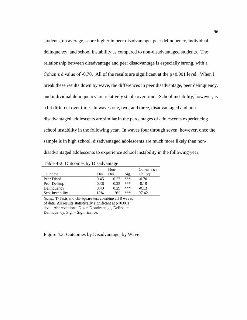
96

students, on average, score higher in peer disadvantage, peer delinquency, individual

delinquency, and school instability as compared to non-disadvantaged students. The

relationship between disadvantage and peer disadvantage is especially strong, with a

Cohen’s d value of -0.70. All of the results are significant at the p<0.001 level. When I

break these results down by wave, the differences in peer disadvantage, peer delinquency,

and individual delinquency are relatively stable over time. School instability, however, is

a bit different over time. In waves one, two, and three, disadvantaged and non-

disadvantaged adolescents are similar in the percentages of adolescents experiencing

school instability in the following year. In waves four through seven, however, once the

sample is in high school, disadvantaged adolescents are much more likely than non-

disadvantaged adolescents to experience school instability in the following year.

Table 4-2: Outcomes by Disadvantage

Outcome Dis.

Non-

Dis. Sig.

Cohen’s d /

Chi Sq.

Peer Disad. 0.45 0.23 *** -0.70

Peer Delinq. 0.36 0.25 *** -0.19

Delinquency 0.40 0.29 *** -0.13

Sch. Instability 13% 9% *** 97.42

Notes: T-Tests and chi-square test combine all 8 waves

of data. All results statistically significant at p<0.001

level. Abbreviations: Dis. = Disadvantage, Delinq. =

Delinquency, Sig. = Significance.

Figure 4.3: Outcomes by Disadvantage, by Wave

97

Multivariate Analyses

Disadvantage Predicting Four Outcomes

I estimated four multivariate, multilevel regression models in which disadvantage

separately predicts peer disadvantage, peer delinquency, individual delinquency, and

school instability when controlling for grades, school bonding, family relations,

unstructured socializing, sex, race, wave, treatment condition. This provides a baseline

relationship between disadvantage and the four outcomes to determine if there is a

0.000.100.200.300.400.500.60

W1 W2 W3 W4 W5 W6 W7 W8

Peer Disadvantage

Disad Non-Disad

0.000.100.200.300.400.500.60

W1 W2 W3 W4 W5 W6 W7 W8

Peer Delinquency

Disad Non-Disad

0.000.100.200.300.400.500.60

W1 W2 W3 W4 W5 W6 W7 W8

Delinquency

Disad Non-Disad

0%

10%

20%

30%

W1 W2 W3 W4 W5 W6 W7

School Instability

Disad Non-Disad

98

relationship to be explored further. Presented in Table 4.3, these results demonstrate that

disadvantage is a significant predictor of each of the four outcomes. As disadvantage

increases, levels of peer disadvantage, peer delinquency, individual delinquency, and

likelihood of school instability are expected to increase, while controlling for grades,

school bonding, family relations, unstructured socializing, sex, race, wave, and treatment

condition.

[Table 4.3: Disadvantage Predicting Peer Disadvantage, Peer Delinquency, Delinquency,

and School Instability about here]

Next, I will conduct mediation tests to determine if the social measures mediate

the relationship between disadvantage and any of the four outcomes. To do so, I must

first assess path a of the mediation diagram.

Path a: Mediation Measures as Outcomes

Table 4.4 presents the results when examining paths a of the mediation models.

In other words, each of the social measures is treated as the outcome variable with

disadvantage as the primary predictor. As noted in Chapter 3, this is one of two

relationships that must come together to create mediation: the stronger this relationship,

the greater potential for that variable to mediate its impact on the outcome. These

relationships were also addressed in in Chapter 3, but I return to them here in a version

more closely matched to their role in this chapter. First, I include previous and current

isolates in addition to Bonacich centrality, stability, and reciprocity. Additionally, in this

chapter I use the in-school sample, whereas the previous chapter only used the in-home

sample. Each three-level, multilevel model controls for school grades, school bonding,

99

family relations, unstructured socializing, sex, race, wave, and treatment condition.

Consistent with the preceding analyses, disadvantage is a significant predictor of each of

the social measures, and it has the strongest relationship with Bonacich centrality as

compared to the other social measures, implying that Bonacich centrality has the most

potential to be a mediating variable.

[Table 4.4: Path a of Mediation Analysis; Mediators as Outcomes about here]

Peer Disadvantage and Peer Delinquency

Next, I examine if the social measures mediate the relationships between

disadvantage and peer disadvantage and peer delinquency. To reiterate, because peer

disadvantage and peer delinquency are calculated by averaging the measures of one’s

friends, the isolates—previous and current—are excluded from this section of analysis.

Therefore, the potential mediating social variables include Bonacich centrality, friendship

stability, and friendship reciprocity. For each section of analysis, Model I presents the

results from the earlier analysis of disadvantage predicting the outcome when controlling

for school grades, school bonding, family relations, unstructured socializing, sex, race,

wave, and treatment condition. Then, Model II presents the results when including the

mediating variables.

Peer Disadvantage. Table 4.5 presents the results when treating peer

disadvantage as the outcome variable. After including Bonacich centrality, friendship

stability, and friendship reciprocity, the coefficient for individual disadvantage decreases

by approximately 8%. Bonacich centrality and friendship reciprocity are both

100

significantly and negatively related to peer disadvantage. School grades and levels of

peer disadvantage are negatively related, with each increase in the grades resulting in an

expected decrease of 0.028 in levels of peer disadvantage. Males, on average, have lower

levels of peer disadvantage than females. Whites, on average, have lower levels of peer

disadvantage than non-whites. School bonding, family relations, unstructured

socializing, and treatment condition are not significantly related to peer disadvantage,

when controlling for everything else in the final model.

Bonacich centrality is a significant mediator of the relationship between

individual disadvantage and peer disadvantage, accounting for about 6% of the

relationship. Friendship reciprocity is also statistically significant, but accounts for less

than 1% of mediation. Friendship stability is not a significant mediator of the

relationship. In total, the effects from the three social measures account for almost 7%

mediation, and are statistically significant at the p < 0.001 level.

[Table 4.5: Disadvantage Predicting Peer Disadvantage, about here]

Peer Delinquency. Table 4.6 presents the results when treating peer delinquency

as the outcome variable. Model I presents the results from the earlier analysis of

disadvantage predicting peer delinquency when controlling for grades, school bonding,

family relations, unstructured socializing, sex, race, wave, and treatment condition. Upon

including the three social measures, the coefficient for disadvantage decreases by about

9%, but remains significantly related to peer delinquency. Bonacich centrality and

friendship stability are both negative predictors of peer delinquency. Friendship

reciprocity is not a statistically significant predictor of peer delinquency. School grades,

school bonding, and family relations are all negative predictors of peer delinquency,

101

while unstructured socializing is positively related to peer delinquency. Males are more

likely to have delinquent friends as compared to females. Whites are less likely than non-

whites to have delinquent friends. Treatment condition is not statistically significant in

these analyses.

Next, I calculated the indirect effects and significance values for each of the three

social measures. Bonacich centrality and friendship stability are both significant

mediators of the relationship between disadvantage and peer delinquency. Bonacich

centrality accounts for about 6% mediation, while friendship stability accounts for about

3.5%. Friendship reciprocity is not a statistically significant mediator. In total, the three

social measures account for about 9% mediation, and the combined effects are

statistically significant at the p < 0.001 level.

[Table 4.6: Disadvantage Predicting Peer Delinquency, about here]

Delinquency and School Instability

Next, I complete the mediation analyses when delinquency and school instability

are the outcome variables. For this section of analysis, I include previous isolates and

current isolates, as well as peer disadvantage and peer delinquency, as mediating

variables in addition to Bonacich centrality, friendship stability, and friendship

reciprocity. For each section of analysis, Model I presents the results from the earlier

analysis of disadvantage predicting the outcome when controlling for school grades,

school bonding, family relations, unstructured socializing, sex, race, wave, and treatment

condition. Then, Model II presents the results when including the mediating variables.

102

Delinquency. Table 4.7 present the results when treating delinquency as the

outcome variable. The coefficient for disadvantage decreases by about 17% after

including the mediating variables, but disadvantage still remains significantly related to

delinquency. Bonacich centrality is actually positively related to delinquent involvement.

Having higher friendship stability rates is predictive of less delinquent involvement.

Previous isolates are significantly more likely than non-previous isolates to engage in

delinquent behavior. However, current isolates are not significantly more likely to be

delinquent as compared to non-current isolates. Peer delinquency and individual

delinquency are positively and significantly related. Friendship reciprocity and peer

disadvantage are not significant predictors of individual delinquency. All of the control

variables, with the exception of treatment condition, are significantly related to

delinquency.

Next, I calculated the indirect effects and significance values for each of the

mediating variables. Interestingly, Bonacich centrality is a significant mediator of the

relationship between disadvantage and delinquency, but it is acting as a suppressor effect

(more on this below). Friendship stability and previous isolates are both significant

mediators of the relationship between disadvantage and delinquency, accounting for

about 2% and 3% of the relationship, respectively. Peer delinquency is the strongest

mediator of the relationship, accounting for almost 13% of the relationship between

disadvantage and delinquency. Friendship reciprocity, current isolates, and peer

disadvantage are not significant mediators. In total, the mediating variables account for

about 14% mediation, and are statistically significant at the p < 0.01 level.

103

To help understand the suppressor effect with Bonacich centrality, I estimated

additional models. First, I estimated a model that included disadvantage, the five social

measures (including two isolates), and only the demographic measures as control

variables. In other words, this model did not include peer disadvantage and peer

delinquency as mediators, or grades, school bonding, family relations, and unstructured

socializing as controls. In this model, Bonacich centrality was negatively related to

delinquency, and was a significant mediator of the relationship between disadvantage and

delinquency (Coef. = -0.018, RSE = 0.006; 2.4% mediation, p<0.01). This demonstrates

that the overall contribution of Bonacich centrality is in expected direction, even if

further intervening relationships to other variables leave it with a direct effect in the

unexpected direction.

Then, I wanted to separate the effects of peer disadvantage and peer delinquency

to understand more how these measures are influencing individual delinquency. I

estimated an additional model that included peer disadvantage, but left out peer

delinquency. In this model, peer disadvantage is significantly related to delinquency

(Coef. = 0.027, RSE = 0.009), and is a significant mediator of the relationship between

disadvantage and delinquency (5.3%, p<0.01), meaning that it matters by its association

with peer delinquency (correlation between peer disadvantage and peer delinquency r =

0.10).

[Table 4.7: Disadvantage Predicting Delinquency, about here]

School Instability. Table 4.8 presents the results when treating school instability

as the outcome variable. As a reminder, school instability is a binary variable so these

are Bernoulli-specified multilevel models with logistic coefficients. Disadvantage

104

remains a significant predictor of school instability, with each one-unit increase in

disadvantage increasing the odds of school instability by about 16%. Bonacich centrality,

friendship stability, and friendship reciprocity are all negatively related to experiencing

school instability. Each one-unit increase in Bonacich centrality decreases the odds of

school instability by almost 50%. A one-unit increase in friendship stability decreases

the odds of school instability by about 17%, while a one-unit increase in friendship

reciprocity decreases the odds by about 36%. However, it is important to consider that a

unit for stability and reciprocity is the difference between 0% and 100%, which are the

two extremes for these variables. Previous isolates, current isolates, peer disadvantage,

and peer delinquency are all positively related to school instability. All of the control

variables, with the exception of treatment condition, are significantly related to school

instability.

Next I calculated the indirect effects and confidence intervals for each of the

mediating variables. All of the mediating variables are significant mediators of the

relationship between disadvantage and school instability. The largest source of mediation

comes from Bonacich centrality, which accounts for about 20% mediation. The next

largest are previous isolates and peer disadvantage, which each account for about 4%.

Friendship reciprocity accounts for about 2.5% mediation, while peer delinquency,

current isolates, and friendship stability all hover around 1% mediation. In total, the

mediating effects account for about 35% mediation, and are statistically significant at the

p < 0.001 level.

[Table 4.8: Disadvantage Predicting School Instability, about here]

105

Discussion

This chapter empirically examined the consequences of the disparity in social

relations between financially disadvantaged adolescents and non-disadvantaged

adolescents. To start, it is evident from the results that financially disadvantaged

adolescents are more likely than non-disadvantaged adolescents to have peers who are

more disadvantaged and to have peers that engage in higher amounts of delinquency.

Next, I determined that popularity is a significant mediator of both of these relationships.

This finding is supportive of criminological theory, especially subcultural theory.

As discussed previously, subcultural theories of delinquency argue that financially

disadvantaged adolescents are less likely to achieve status in the eyes of their peers,

which in turn makes it more likely that they will become friends with other financially

disadvantaged and maladjusted adolescents, especially delinquent peers. My findings are

consistent with this sequence described in subcultural theory. Financially disadvantaged

adolescents are less likely than non-disadvantaged adolescents to be popular within their

social networks, and in turn they are more likely than non-disadvantaged adolescents to

have peers with greater average disadvantage and greater average delinquency.

Criminological theory, as well as theories in education, argue that these

relationships will have important consequences for individual behavior, specifically

individual delinquency and school instability. Starting with theories about individual

delinquency, subcultural theory would argue that increased interactions with

disadvantaged and/or delinquent adolescents should lead to individual involvement in

delinquency. Their low social status will motivate these disadvantaged adolescents

106

would to attempt to gain status with new friends, and the most likely candidates will also

be disadvantaged and have a higher chance of engaging in delinquency. As discussed in

detail in chapter 1, previous research has demonstrated that aggressive/or delinquent

children tend to be on the periphery of their social networks (Coie et al. 1982; McGuire

1973). Thus, I argued that if disadvantaged adolescents are less likely to be popular, then

this might cause an increase in the likelihood that they will come into contact with

delinquent peers. Differential association theory, then, would argue that, because of this

higher association with delinquent peers, this should lead to higher levels of individual

delinquency.

The findings from this chapter and the previous chapter support these theoretical

arguments. First, popularity is a significant mediator of the relationship between

disadvantage and individual delinquency, prior to including peer disadvantage and peer

delinquency. Then, after including peer disadvantage and peer delinquency, the

mediating effect of popularity is accounted for, and even switches directions. In other

words, disadvantaged adolescents are less likely to be popular, which in turn causes them

to associate more with disadvantaged and delinquent peers. This higher association with

disadvantaged and delinquent peers is causing the individual to engage in more

delinquency, supporting expectations from both subcultural theories and differential

association. Though these results support theoretical arguments, it should be noted that a

limitation of my analyses is that there is a chance that the causal ordering may be

reversed. In other words, it is possible that disadvantaged adolescents are engaging in

delinquency, which in turn causes them to seek out other delinquent peers. This is an

area that future research should address.

107

As discussed in chapter 1, Rumberger and Larson (1998) determine that students

transferring schools just one time between 8th and 12th grade were twice as likely as

students who did not transfer schools to experience future dropout. With research

demonstrating clear links between disadvantage and school instability (Rumberger 1987;

Kolstad and Owings 1986), understanding why this relationship exists is crucial.

Rumberger (1987) explained that the reasons for students dropping out of school are

varied, but can generally be grouped into several major categories, two of which are

school-related and peer-related.

The findings from this chapter demonstrate that all five of the social measures, as

well as peer disadvantage and peer delinquency, are significant mediators of the

relationship between disadvantage and school instability. This pattern holds even after

accounting for academic measures (e.g., school grades, school bonding). These findings

support the theoretical arguments of Wehlage and colleagues (1989), specifically that

researchers should focus on not only on the academic aspects of school belonging, but

only on its social dimensions. This chapter expands on these theoretical arguments by

demonstrating that social success is an important mediator of disadvantage and school

instability. This dissertation extends this area of research by concluding that popularity,

stable friendships, reciprocal friendships, social isolation, disadvantaged friends, and

delinquent friends all have separate and significant mediating effects on the relationship

between disadvantage and school instability.

108

Table 4-3: Baseline Multivariate Models of Disadvantage Predicting Four Outcomes.

Peer Disad. Peer Delinq Delinquency Sch. Instability

Coef. RSE Coef. RSE Coef. RSE O.R. Coef. RSE

Disadvantage 0.051 0.001 *** 0.021 0.002 *** 0.023 0.003 *** 1.313 0.272 0.015 ***

Grades -0.032 0.002 *** -0.068 0.004 *** -0.079 0.004 *** 0.610 -0.494 0.024 ***

School Bonding -0.004 0.003 ** -0.094 0.005 *** -0.270 0.005 *** 0.759 -0.276 0.031 ***

Family Relations -0.008 0.004

-0.065 0.008 *** -0.334 0.008 *** 0.891 -0.115 0.049 *

Unstr.Socializing 0.000 0.001 * 0.036 0.003 *** 0.046 0.003 *** 1.076 0.073 0.017 ***

Male -0.028 0.004 *** 0.114 0.007 *** 0.112 0.010 *** 0.915 -0.089 0.045 *

White -0.077 0.006 *** -0.063 0.011 *** -0.089 0.013 *** 0.709 -0.344 0.056 ***

Wave -0.023 0.001 *** 0.045 0.001 *** 0.027 0.001 *** 1.404 0.340 0.016 ***

Treatment 0.001 0.001

0.001 0.003

0.000 0.000

1.000 0.000 0.000

Constant 0.592 0.014 *** 0.599 0.026 *** 1.389 0.027 ***

-1.286 0.160 ***

Notes: *p<0.05, **p<0.01, ***p<0.001. Level 1 N = 36,820/36,937/56,166/48,997, Level 2 N = 10,748/10,756/14,552/13,969, Level 3 N = 54.

Abbreviations: Coef. = Coefficient, RSE = Robust Standard error, O.R. = Odds Ratio, Disad. = Disadvantage, Delinq = Delinquency, Sch. =

School. Female is the reference variable to male. Non-white is the reference variable to white.

109

Table 4-4: Path a of Mediation Analysis; Mediating Variables as Outcomes.

Predictor Mediator as Outcome Coef. RSE.

Disadvantage Bonacich Centrality -0.072 0.003 ***

Stability Rate -0.010 0.001 ***

Reciprocity Rate -0.015 0.001 ***

Previous Isolate 0.025 0.001 ***

Current Isolate 0.013 0.001 ***

Notes:*p<0.05, **p<0.01, ***p<0.001. Level 1 N=59,589; Level 2 N= 14,622, Level 3

N=54. Abbreviations: Coef. = Coefficient; RSE = Robust Standard Error. All models are 3-

level, multilevel models that controlled for grades, school bonding, family relations,

unstructured socializing, sex, race, wave, and treatment condition.

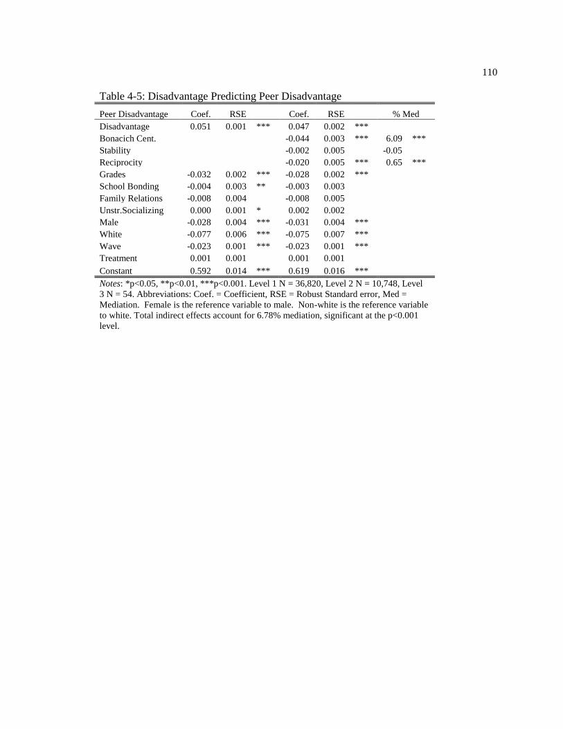
110

Table 4-5: Disadvantage Predicting Peer Disadvantage

Peer Disadvantage Coef. RSE Coef. RSE % Med

Disadvantage 0.051 0.001 *** 0.047 0.002 ***

Bonacich Cent.

-0.044 0.003 *** 6.09 ***

Stability

-0.002 0.005

-0.05

Reciprocity

-0.020 0.005 *** 0.65 ***

Grades -0.032 0.002 *** -0.028 0.002 ***

School Bonding -0.004 0.003 ** -0.003 0.003

Family Relations -0.008 0.004

-0.008 0.005

Unstr.Socializing 0.000 0.001 * 0.002 0.002

Male -0.028 0.004 *** -0.031 0.004 ***

White -0.077 0.006 *** -0.075 0.007 ***

Wave -0.023 0.001 *** -0.023 0.001 ***

Treatment 0.001 0.001

0.001 0.001

Constant 0.592 0.014 *** 0.619 0.016 ***

Notes: *p<0.05, **p<0.01, ***p<0.001. Level 1 N = 36,820, Level 2 N = 10,748, Level

3 N = 54. Abbreviations: Coef. = Coefficient, RSE = Robust Standard error, Med =

Mediation. Female is the reference variable to male. Non-white is the reference variable

to white. Total indirect effects account for 6.78% mediation, significant at the p<0.001

level.

111

Table 4-6: Disadvantage Predicting Peer Delinquency

Model I Model II

Peer Delinquency Coef. RSE Coef. RSE % Med.

Disadvantage 0.021 0.002 *** 0.019 0.002 ***

Bonacich Cent.

-0.018 0.005 *** 6.22 ***

Stability

-0.078 0.010 *** 3.67 ***

Reciprocity

0.007 0.010

-0.58

Grades -0.068 0.004 *** -0.065 0.005 ***

School Bonding -0.094 0.005 *** -0.092 0.006 ***

Family Relations -0.065 0.008 *** -0.062 0.009 ***

Unstr.Socializing 0.036 0.003 *** 0.035 0.003 ***

Male 0.114 0.007 *** 0.116 0.007 ***

White -0.063 0.011 *** -0.061 0.012 ***

Wave 0.045 0.001 *** 0.045 0.002 ***

Treatment 0.001 0.003

0.021 0.090

Constant 0.599 0.026 *** 0.622 0.029 ***

Notes: *p<0.05, **p<0.01, ***p<0.001. Level 1 N = 36,937 Level 2 N = 10,756 Level 3 N =

54. Abbreviations: Coef. = Coefficient, RSE = Robust Standard error, Med = Mediation.

Female is the reference variable to male. Non-white is the reference variable to white. Total

indirect effects account for 9.32% mediation, significant at the p<0.001 level.

112

Table 4-7: Disadvantage Predicting Delinquency

Model I Model II

Delinquency Coef. RSE Coef. RSE % Med.

Disadvantage 0.023 0.003 *** 0.019 0.003 ***

Bonacich Cent.

0.015 0.006 * -5.65 *

Stability

-0.042 0.011 *** 1.63 ***

Reciprocity

-0.005 0.010

0.36

Previous Isolate

0.024 0.007 *** 3.07 ***

Current Isolate

0.004 0.011

0.28

Peer Disadvantage

0.008 0.010

1.90

Peer Delinquency

0.162 0.006 *** 12.77 ***

Grades -0.079 0.004 *** -0.072 0.005 ***

School Bonding -0.270 0.005 *** -0.259 0.007 ***

Family Relations -0.334 0.008 *** -0.328 0.011 ***

Unstr.Socializing 0.046 0.003 *** 0.042 0.003 ***

Male 0.112 0.010 *** 0.095 0.010 ***

White -0.089 0.013 *** -0.078 0.014 ***

Wave 0.027 0.001 *** 0.021 0.002 ***

Treatment 0.000 0.000

0.000 0.000

Constant 1.389 0.027 *** 1.308 0.034 ***

Notes: *p<0.05, **p<0.01, ***p<0.001. Level 1 N = 56,166, Level 2 N = 14,552, Level 3 N = 54.

Abbreviations: Coef. = Coefficient, RSE = Robust Standard error, Med = Mediation. Female is the

reference variable to male. Non-white is the reference variable to white. Total indirect effects account

for 14.30% mediation, significant at the p<0.001 level.

113

Table 4-8: Disadvantage Predicting School Instability

Model I Model II

School Instability O.R. Coef. RSE O.R. Coef. RSE % Med

Disadvantage 1.313 0.272 0.015 *** 1.162 0.150 0.013 ***

Bonacich Cent.

0.508 -0.676 0.048 *** 20.75 ***

Stability

0.824 -0.193 0.080 * 0.63 *

Reciprocity

0.638 -0.449 0.060 *** 2.59 ***

Previous Isolate

1.470 0.385 0.041 *** 4.24 ***

Current Isolate

1.229 0.206 0.050 *** 1.15 ***

Peer Disadvantage

1.229 0.206 0.056 *** 4.01 ***

Peer Delinquency

1.239 0.214 0.030 *** 1.62 ***

Grades 0.610 -0.494 0.024 *** 0.697 -0.361 0.023 ***

School Bonding 0.759 -0.276 0.031 *** 0.829 -0.187 0.029 ***

Family Relations 0.891 -0.115 0.049 * 0.880 -0.128 0.047 **

Unstr.Socializing 1.076 0.073 0.017 *** 1.092 0.088 0.016 ***

Male 0.915 -0.089 0.045 * 0.789 -0.236 0.040 ***

White 0.709 -0.344 0.056 *** 0.837 -0.178 0.050 ***

Wave 1.404 0.340 0.016 *** 1.266 0.236 0.014 ***

Treatment 1.000 0.000 0.000

1.000 0.000 0.000

Constant

-1.286 0.160 ***

-1.087 0.155 ***

Notes: *p<0.05, **p<0.01, ***p<0.001. Level 1 N = 48,997, Level 2 N = 13,969, Level 3 N = 54.

Abbreviations: O.R. = Odds Ratio, Coef. = Coefficient, RSE = Robust Standard error, Med = Mediation.

Female is the reference variable to male. Non-white is the reference variable to white. Total indirect

effects account for 34.99% mediation, significant at the p<0.01 level.

114

Chapter 5

Adolescent Social Relations and Young Adulthood Adjustment

The previous chapters of this dissertation have demonstrated that financially

disadvantaged adolescents are less likely than non-disadvantaged adolescents to be well

integrated within their school-based social networks, and that this disparity in social

relations has important short-term consequences. This chapter of my dissertation

examines the extent to which the disparity in social relations affects young adult

adjustment, specifically in regards to educational attainment. A growing field of research

is examining the long-term effects of adolescent friendships, such as how the

development of socioemotional traits during adolescence may help to explain adulthood

economic, educational, and health behaviors (Bowles, Herbert, and Osborne 2001; Cunha

et al. 2006). Studies have shown that popularity and friendships during adolescence are

connected to outcomes in young adulthood, such as life adjustment (Bagwell, Newcomb,

and Bukowski 2008) and income (Shi and Moody 2017).

However, existing research has not explored the relationship between

disadvantage, adolescent social status, and educational attainment. Interest in attending

college is near universal (Kuh and colleagues 2006), but adjustment to and succeeding

within college is dependent on numerous factors. One of these factors that is important to

consider is social engagement. Relatedly, friendships and social acceptance during

adolescence pave the way for one’s ability to successfully socialize in adulthood (Berndt

1982). Therefore, I argue that adolescent social acceptance will be related to young-

115

adulthood educational attainment, and will mediate the relationship between family

background and educational attainment. Additionally, it is unclear if peer acceptance is

the only aspect of social relations that affects future adjustment, or if other social

measures (e.g., stability, reciprocity) also have an impact. Thus, I will include measures

of average high school stability and average high school reciprocity in my analyses.

Finally, subcultural theories of juvenile delinquency argue that, especially for

disadvantaged adolescents, the type of friends one has during adolescence will have

important consequences for individual behavior and adjustment. Staff and Kreager

(2008) empirically supported this argument, concluding that gaining status in violent

groups had a detrimental impact on high school completion, but only for disadvantaged

males. Therefore, I will also consider the type of friends, relative to disadvantage and

delinquent involvement, one is gaining when considering the impact of adolescent social

relations. This chapter addresses my third research question: does the disparity in social

success between disadvantaged adolescents and non-disadvantaged adolescents partially

mediate the relationship between disadvantage and educational attainment?

In this chapter, I consider whether Bonacich centrality, friendship stability, and/or

friendship reciprocity are partial mediators of the relationship between disadvantage and

educational attainment. Additionally, I consider whether levels of disadvantage and

delinquency among one’s adolescent friendships impacts educational attainment. Figure

5.1 presents a path diagram that demonstrates the focus of the current chapter. I

hypothesize that adolescent social relations will partially mediate the relationship

between disadvantage and college attainment.

116

Figure 5-1: Path diagram demonstrating the focus of this chapter.

Methodology

PROSPER Data

In-School and Follow-up Sample. I use longitudinal social network data from the

evaluation of the PROmoting School-community-university Partnerships to Enhance

Resilience (PROSPER) longitudinal study (Spoth et al. 2007; please see Chapter 2 for

more information about the sample). While I will use the in-school data to create an

average of high school social relations for each individual, my analysis will be based on a

subsample of the PROSPER data set that was asked to complete a follow-up survey at

approximately age 24 to determine educational attainment (please see Chapter 2 for more

information). The final sample size for this chapter is 727.

I conducted comparison of means tests on key measures that compared the

follow-up sample to the main in-school sample and found some significant differences

between the two samples. I argue that this is likely because it has been demonstrated in

other studies that the likelihood of responding to surveys are correlated with specific

variables, such as education and socioeconomic status (Kwak and Radler 2002; Dillman

et al. 2009; Tolonen et al. 2006). Considering that the in-school surveys had higher

response rates than the follow-up survey, it would be expected that the average

117

respondent in the follow-up survey may be a bit different than the average respondent of

the in-school sample. The results of the comparison of means test indicate a similar

pattern, in that the follow-up sample consists of young adults that were, on average, less

disadvantaged adolescents than the average of the in-school sample. Similarly, those

responding to the survey in young adulthood were higher, on average, than the in-school

average in Bonacich centrality, in-degree, reciprocity, stability, and grades. The

differences in rates of disadvantage and social integration are not so large that there is

any reason to suspect they would introduce any in my results. Nevertheless, these

differences may reduce variation on these key factors, which would have the potential to

reduce statistical power somewhat.

Measures

Table 5.1 provides a description and descriptive statistics for all of my measures.

High school variables are all mean measures that averaged values from ninth through

twelfth grade.

Table 5-1: Descriptive Statistics.

Measure Description Mean SD Min Max

Educational Attainment Measured at the follow-up

survey; indicates whether or

not the respondent has

attained a four-year degree.

0.44 0.00 1.00

Disadvantage Empirical Bayes aggregate

of student-reported receiving

of free/reduced price lunch.

-0.55 1.55 -1.72 3.43

Bonacich Centrality Indicator of the number and

prestige of the friends that

the actor is connected to;

averaged from 9th through

12th grade.

0.86 0.52 0.00 2.78

118

Stability Rate Proportion of friends from

T1 that overlap to T2;

averaged from 9th through

12th grade.

0.42 0.23 0.00 1.00

Reciprocity Rate Proportion of mutual to non-

mutual friendships; averaged

from 9th through 12th grade.

0.54 0.27 0.00 1.00

Peer Disadvantage The average of empirical

Bayes FRL disadvantage

across each of the friends of

a given respondent

-0.54 1.01 -1.70 3.21

Peer Delinquency Average of friends'

delinquency (IRT scale).

0.38 0.48 -0.34 2.48

Grades Student-reported school

grades; averaged from 9th

through 12th grade.

4.19 0.78 1.00 5.00

Absences Number of absences for a

given school year; averaged

from 9th through 12th grade.

3.04 0.88 1.00 5.00

Family Relations Mean of standardized

subscales assessing family

relations; averaged from 9th

through 12th grade.

-0.18 0.37 -1.25 0.73

Mental Health Composite measure

assessing depression and

anxiety; averaged from 9th

through 12th grade.

0.36 0.41 0.00 2.00

Expresses Opinion Self-reported ability of the

respondent to express his/her

opinion; averaged from 9th

through 12th grade.

1.81 0.79 1.00 5.00

Delinquency 12-item index of

delinquency behavior (IRT

scale); averaged from 9th

through 12th grade.

0.46 0.77 -0.34 3.94

Unstr. Socializing Average of time spent with

individuals nominated as

friends; averaged from 9th

through 12th grade.

2.78 0.97 0.00 5.00

Male Whether respondent is male

or female. 1=Male;

0=Female.

0.43 0.50 0.00 1.00

White Whether respondent is white

or non-white. 1=White;

0=Non-white.

0.88 0.33 0.00 1.00

Wave The year the survey was

administered.

22.95 0.46 22.00 25.00

Treatment Whether or not the given

school received the

treatment intervention.

0.48 0.00 1.00

119

Educational Attainment. This measure indicates whether or not the respondent

has attained a four-year degree. In the follow-up survey, respondents were asked, “what

is the highest education degree or certificate you hold?” I have recoded educational

attainment so that it is a binary measure of attaining a four-year college degree. I also

completed sensitivity analyses using other versions of this measure. This binary measure

is coded as 1 if the respondent has attained a four-year college degree, and a 0 if not. At

the time of follow-up survey, 44% of the sample had attained a four-year degree.

Financial Disadvantage. This chapter uses the empirical Bayes FRL measure of

disadvantage, the same measure for financial disadvantage as the previous two chapters.

For a more detailed description of this measure, please see Chapter 2 of this dissertation.

Financial disadvantage has an average score of -0.55, with a standard deviation of 1.55.

Average High School Bonacich Centrality. Using the PROSPER in-school social

network data, I measure each respondent’s average high school Bonacich centrality by

averaging together the Bonacich centrality scores across high school. Sensitivity

analyses were also completed using in-degree as the social acceptance measure, and are

presented after the main results. Bonacich centrality is calculated by weighting each

node’s centrality by the centrality of the actors that they are connected to. In other words,

an individual gets an increase in Bonacich centrality if he/she is tied to other individuals

who are central within the network. Each student receives a Bonacich centrality score at

each wave of data collection. By averaging together each respondent’s ninth through

twelfth grade Bonacich centrality scores, I have a mean measure for high school

popularity. Those individuals that did not have data for Bonacich centrality in any of the

120

waves were coded as missing and not included in the analyses. There was only limited

variation in the number of waves and data available, as almost 80% of the sample had 3

or 4 waves of information to average from, and only 7% had only one wave of

information. As discussed in the previous chapter, I also could have used in-degree as a

measure of popularity. However, in-degree and Bonacich centrality are strongly

correlated (r=0.75), and Bonacich centrality gives more information about an individual

regarding his/her standing in the social network, so I use Bonacich centrality as the sole

measure of popularity for this chapter. The mean of the average high school popularity

measure is 0.86, with a standard deviation of 1.55.

Average High School Stability Rate. Friendship stability is a rate that is

calculated by dividing the number of repeated nominations received in T2 by the number

of total nominations received in T1. These rates were calculated at each wave of high

school, and then averaged together to create an average high school stability rate for each

respondent. The mean for average stability rate is 0.42, with a standard deviation of 0.23.

Because this is a proportion, the range of the variable is 0 to 1. The mean of 0.42

indicates that, on average, about 42% of respondents’ friendship nominations were stable

from one year to the next during high school.

Average High School Reciprocity Rate. Friendship reciprocity is a rate that is

calculated as the number of reciprocated friendships divided by the number of sent

nominations. These rates were calculated at each wave of high school, and then averaged

together to create an average high school reciprocity rate for each respondent. The mean

for average reciprocity rate is 0.54 with a standard deviation of 0.27. Similar to stability,

121

the range is 0 to 15. This mean score of 0.54 indicates that, on average, about 54% of

respondents’ friendship nominations were reciprocated during high school.

Average Peer Disadvantage. Average peer disadvantage is an average of the

average Bayes FRL measure from the respondents’ friends from each wave of high

school. As previously discussed, the PROSPER Peers data set includes friendship

nominations that were matched to the students, which allows researchers to create a full

social network of the cohort. The peer disadvantage measure uses the scores of the

friends on the empirical Bayes FRL variable to create an average disadvantage score for

those friends. The average peer disadvantage measure then averages each of these scores

together to create an average from high school. The average respondent has a mean peer

disadvantage score of -0.54 with a standard deviation of 1.01.

Average Peer Delinquency. The Average Peer Delinquency measure is an

average of the Average IRT delinquency measure from the respondents’ friends that was

calculated at each wave of high school. Again, this measure is created using the full

social network of the cohort. This alleviates projection bias (Young et al. 2013), which is

when students inaccurately project their own behavior when describing the behavior of

their friends. Because the PROSPER Peers project provides matched nominations, I am

able to employ an average peer delinquency measure based on a respondent’s friends’

own IRT delinquency scores. This was completed for each wave of high school, which

were then averaged together across high school to create the average peer delinquency

5 As discussed in the previous chapter, isolates will be excluded from the analysis when using

stability rate and reciprocity rate. However, in this chapter’s sample, there are only 15 individuals who

qualify as isolates when averaging information from all waves of data in high school. Therefore, there

would be too few cases to include average isolates as another social measure in this analysis.

122

measure. The average value of average peer delinquency is 0.38 with a standard

deviation 0.48 and a range of -0.34 to 2.48.

Controls. The control variables are high school grades, absences, family

relations, mental health, ability to express opinions, delinquency, unstructured

socializing, sex, race, and treatment condition. All of the control variables, with the

exception of sex, race, and treatment condition, are means of data from ninth through

twelfth grade. Sex, race, and treatment condition did not vary from year-to-year for any

of the respondents in this sample. High school grades, absences, family relations,

delinquency, and unstructured socializing are all measures used in previous chapters.

Mental health is a scale (a=0.91) made up of 10 items that assesses anxiety and

depression. This scale has a mean score of 0.36, standard deviation of 0.41, and a range

of 0 to 2. At each wave of in-school data, the adolescents were asked the likelihood that

they would express an opinion even though others may disagree with them. Responses

ranged from definitely would, coded as 1, to definitely would not, coded as 5. The

average score of expresses opinion is a 1.81, with a standard deviation of 0.79.

Sex is a binary variable coded as 0 for female and 1 for male. Race is a binary

variable coded as 0 for non-white and 1 for white6. Age is the age of the respondent at

the time of the follow-up survey. Treatment condition is a variable that is included to

control for between-school differences of whether or not that school received a substance

use intervention as part of the larger PROSPER study (see Spoth et al. 2007 for more

information).

6 Similar to previous chapters, there are too few non-whites (10%) in this sample to break non-

whites down into additional categories.

123

Analytic Strategy

In the previous chapters, the data structure had three levels: wave was nested

within individuals that were nested within communities. The current chapter does not

have multiple waves, but I still must account for the nesting of individuals within

communities. Due to this clustering nature of my dataset, I will rely upon hierarchical

linear modeling using HLM software (Bryk and Raudenbush 2002) to address my

research questions. The data are clustered within communities, meaning that students

that are from the same community are not statistically independent of one another, as

these students may be more similar to one another as compared to students across

communities. To control for within-community dependence, I will estimate two-level,

multilevel models that nests individuals (level-1) within communities (level-2).

To determine a baseline association between disadvantage and educational

attainment, I will start with a Pearson chi-square test of association. I will then estimate

multivariate, multilevel model of disadvantage predicting educational attainment,

inclusive of the control variables. Then, I will estimate mediation analyses to determine

if the relationship between disadvantage and educational attainment is mediated by the

three social measures. In order to effectively examine if the social measures are

mediating the relationship between disadvantage and educational attainment, once again I

will use the Baron-Kenny framework (Baron and Kenny 1986). First, I will treat the

three social measures and the two types of friends measures as outcome variables, with

disadvantage being the primary predictor variable. These two-level, multilevel models

will include the control variables. This will allow me to assess the relationship between

124

disadvantage and the social measures separately, which will assess path a from the Baron

and Kenny’s (1986) standard conception of mediation. Though these analyses are similar

to those performed in previous chapters, the mediators are averages across waves, the

sample for this chapter is different from the previous chapters, and the control variables

are different. Therefore, to complete the mediation analysis, I return to them here in a

version more closely matched to their role in this chapter.

After assessing path a, I will estimate a two-level Bernoulli-specified model

predicting educational attainment that includes disadvantage, the three social measures,

and my control variables. Then, I will calculate the indirect effects, significance values,

and proportion mediated of the social measures. The indirect effects of the social

measures are calculated using the same method as the previous chapters. The percentage

explained by each social measure is presented with asterisks to indicate significance

values. I will then repeat this process after including peer disadvantage and peer

delinquency into the model.

Results

Bivariate Analysis

My first goal is to document the relationship between an adolescent’s background

and his/her educational attainment. Only 22% of the individuals from a disadvantaged

background have obtained a four-year degree by age 23. Conversely, 52% of individuals

from a non-disadvantaged background have obtained a four-year degree by age 23. This

125

difference is statistically significant at the p<0.001 level (2 = 54.46). Next, I estimate a

multivariate, multilevel model of disadvantage predicting educational attainment that

includes my control variables.

Multivariate Analyses

Disadvantage Predicting Educational Attainment

Table 5.2 presents the results from a two-level Bernoulli model predicting

educational attainment. Disadvantage and educational attainment are significantly and

negatively related. High school grades is the strongest predictor of educational

attainment. High school absences, current mental health, high school church attendance,

current smoking, white, and age are also all significantly related to educational

attainment. Next, I will conduct mediation tests to determine if the social measures,

and/or type of friends, mediate the relationship between disadvantage and educational

attainment. To do-so, I must first assess path a of the mediation diagram.

[Table 5.2, about here]

Path a of Mediation Analysis

Table 5.3 presents the results when assessing path a of the mediation diagram.

For this section, I estimated three separate two-level models that predicted high school

Bonacich centrality, high school stability, and high school reciprocity. Interestingly,

126

disadvantage is only a significant predictor of high school Bonacich centrality,

controlling for everything else in the models. This indicates that, of my three social

relation measures, only high school Bonacich centrality can be a potential mediating

variable. In other words, high school stability and high school reciprocity cannot be

mediators of the relationship between disadvantage and educational attainment.

Disadvantage is a significant predictor of both peer disadvantage and peer delinquency,

indicating that both of these variables can be potential mediating variables. However, the

relationship between disadvantage and peer disadvantage is much stronger than the

relationship between disadvantage and peer delinquency.

[Table 5.3 about here]

Mediation Variables

Social Relations. Table 5.4 presents the results from the two-level, Bernoulli

model predicting educational attainment. The first set of results in the table is included as

a reference to the previous analysis predicting educational attainment. The right-side of

the table includes the results once the social measures were included in the analyses.

After including the three social measures, disadvantage remains negatively related to the

odds of obtaining a four-year degree. High school Bonacich centrality is a significant

predictor of educational attainment, but neither of the other two social measures are

significantly related. High school grades remains the strongest predictor of educational

attainment. High school absences is significantly and negatively related to educational

127

attainment. White respondents are less likely to obtain a four-year degree as compared to

non-whites.

As discussed previously, only high school Bonacich centrality has the potential to

be a significant mediator in these analyses. After calculating the indirect effects,

significance values, and percent mediated of the social measures, high school Bonacich

centrality is a significant mediator, accounting of almost 18% of the relationship between

disadvantage and educational attainment.

[Table 5.4, about here]

Types of Friends. Next, I included peer disadvantage and peer delinquency in the

model, in addition to the three social measures, to determine if the type of friends matter

when examining the relationship of disadvantage and educational attainment. Table 5.5

presents these results. In this model, individual disadvantage is no longer significantly

related to educational attainment, though it still has a substantial coefficient. Bonacich

centrality is still a significant predictor of educational attainment, while stability and

reciprocity are not significantly related. Peer disadvantage is a significant predictor of

educational attainment, while peer delinquency is not. After calculating the indirect

effects, significance values, and percent mediated of the effects of social measures, I

determined that Bonacich centrality and peer disadvantage are both significant mediators

of the relationship between disadvantage and educational attainment. Bonacich centrality

still accounts for about 13% of the relationship, while peer disadvantage accounts for

about 33%.

[Table 5.5 about here]

128

Sensitivity Analyses

I also completed additional analyses to further understand the results of this

chapter. First, Staff and Kreager (2008) demonstrated in their study that the negative

effects of gaining status in a delinquent peer group differentially affected disadvantaged

adolescents. Thus, I split my sample by disadvantage to determine if the effects of the

adolescent social relations and of type of friends varied for disadvantaged adolescents as

compared to non-disadvantaged adolescents. As in previous chapters, I coded the top

15% of the Bayes FRL variable as disadvantaged, with the remaining 85% as non-

disadvantaged.

The effect of Bonacich centrality remained statistically significant for non-

disadvantaged adolescents (Coef. = 0.481; RSE = 0.243), but was not statistically

significant for non-disadvantaged adolescents (Coef. = 0.431; RSE = 0.592). However,

the magnitude of the effect was rather similar for both non-disadvantaged and

disadvantaged adolescents, while the difference in standard errors accounted for the

difference in statistical significance. This indicates that the difference in sample size is

most likely responsible for the difference in statistical significance between the two

samples. Taken together, it seems that the effect of Bonacich centrality on educational

attainment is rather similar for both non-disadvantaged and disadvantaged adolescents.

A similar pattern is evident for the effect of peer disadvantage on educational

attainment for non-disadvantaged adolescents and disadvantaged adolescents. Peer

disadvantage was a significant predictor of educational attainment for non-disadvantaged

adolescents (Coef. = -0.601; RSE = 0.193), but was not statistically significant for in the

129

model of only disadvantaged adolescents (Coef. = -0.603; RSE = 0.443. However, once

again, the magnitude of the effect of peer disadvantage on educational attainment was

similar for both disadvantaged and non-disadvantaged adolescents, indicating that the

differences in statistical significance was most likely due to differences in sample size, as

this increased the standard error in the model of disadvantaged adolescents. Similar to

the primary results presented above for the full sample, peer delinquency was not a

significant predictor in either of the models when the sample was split by disadvantage.

Next, I examined the interaction of Bonacich centrality with peer disadvantage.

This interaction term will reflect the degree that the effect of social acceptance varies

based on the type of friends that the adolescent is gaining status with (Staff and Kreager

2008). This interaction term was not a statistically significant predictor of educational

attainment, nor a significant mediator of the relationship of disadvantage and educational

attainment, when included in the models for the full sample. This result indicates that the

long-term effect of adolescent social acceptance on educational attainment does not vary

based on the levels of peer disadvantage of the social groups that the adolescent was

gaining status within.

Then, I estimated the interaction of Bonacich centrality with peer delinquency.

Even though peer delinquency was not a significant predictor in the model for the full

sample, or when splitting the sample, I wanted to be sure that the effects of social

acceptance are not dependent upon the delinquency of the adolescents’ primary friends.

This interaction term was not statistically significant for the full sample or for either

subsample when the follow-up sample was split by adolescent disadvantage.

Additionally, subcultural theories of juvenile delinquency argue that the effects of social

130

ties and peer delinquency may have differential effects upon boys as compared to girls. I

would have liked to further these analyses by splitting the sample to isolate

disadvantaged boys, but the sample size was too small (n=59) to perform multivariate

analyses (i.e., the estimates had very large standard errors).

Additionally, as I explain in the discussion section of this chapter, a limitation of

this project is that I do not have a measure for adolescent educational aspirations for this

follow-up sample. That is because the question asking about educational aspirations was

only included in the adolescent in-home interviews, and none of the individuals

interviewed at age 24 were included in the adolescent in-home interviews. However,

there is a separate follow-up sample interviewed at age 19. This follow-up sample

included 194 individuals that were also included in the adolescent in-home surveys.

Because this survey was administered when the respondents were approximately 19 years

old, I am not able to assess educational attainment. However, I do have a measure for

educational enrollment. Therefore, I repeated the main analysis of this chapter using this

small sub-sample of 194 individuals but treated college enrollment at age 19 as the

outcome variable with the inclusion of 9th grade educational aspirations as a control

variable. In this model, Bonacich centrality (Coef. = -0.334; RSE = 0.139) is

significantly related to educational enrollment, when controlling for 9th grade

educational aspirations, as well as high school grades, absences, family relations, mental

health, delinquency, unstructured socializing, race, sex, age, and treatment condition.

Meanwhile, 9th grade educational aspirations (coef. = 0.732; RSE = 0.591) was not

significantly related to college enrollment at age 19. These results slightly alleviate the

concern of not having a measure for educational aspirations in my main analyses.

131

I also completed a sensitivity check for the coding of educational attainment. For

this chapter, educational attainment was coded as a binary outcome (i.e., 1 = attaining a

four-year degree and 0 = not attaining a four-year degree). As a sensitivity check, I have

estimated these analyses with educational attainment coded as 0 = none, H.S. graduate,

G.E.D.; 1 = two year college degree or similar; 2 = four-year college degree/Advanced

degree. I then completed the mediation analyses predicting this categorical version of

educational attainment. The results remained similar to the results discussed below when

completing the analyses with educational attainment as a binary variable. More

specifically, in the final models, disadvantage is a significant and negative predictor of

attaining a two-year college degree as compared to a high school degree, and a significant

and negative predictor of attaining a four-year degree as compared to a high school

degree. Of the social measures, Bonacich centrality remained a significant predictor of

attaining a four-year degree as compared to a high school degree, but was not a

significant predictor of attaining a two-year degree as compared to a high school degree.

Bonacich centrality remained a significant mediator of the relationship between

disadvantage and attaining a four-year degree. Neither stability nor reciprocity were

significant predictors or mediators in the final model. These results are very similar to the

main results presented above. In both analyses, Bonacich centrality remained a

significant predictor of attaining a four-year degree. Additionally, in both sets of

analyses, Bonacich centrality was a significant mediator of the relationship between

disadvantage and attaining a four-year degree.

Additional sensitivity analyses treated in-degree as the social acceptance measure

and the results, in general, remained similar to the results above that use Bonacich

132

centrality. More specifically, when assessing path a of the mediation framework,

disadvantage is a significant and negative predictor of average in-degree (Coef. = -0.25,

RSE = 0.05, p = 0.000). In the final model that included disadvantage and the three

social measures predicting educational attainment, disadvantage remained a significant

and negative predictor of educational attainment (Coef. = -0.222, RSE= 0.085, p =

0.009). These values are nearly identical to the values of disadvantage (Coef. = -0.215,

RSE = 0.087, p = 0.013) in the current analyses that include Bonacich centrality. In-

degree is significantly and positively related to educational attainment (Coef. = 0.305,

RSE = 0.066, p = 0.000). Finally, similar to Bonacich centrality, in-degree is a

significant (p<0.001) mediator of the relationship of disadvantage and educational

attainment. The results did differ in the final model in regards to stability and reciprocity.

In the model using in-degree, stability is significant and positively related to educational

attainment (Coef. = 1.069, RSE = 0.468), while reciprocity is significantly and negatively

associated with educational attainment (Coef. = 1.486, RSE = 0.471). Neither of these

two variables are significant mediators, however.

Discussion

This chapter of my dissertation focused on the relationship between disadvantage

and educational attainment in early adulthood, specifically relative to the role of

adolescent social relations. Previous research has demonstrated that disadvantaged

adolescents are less likely to attain a college degree (Sewell and Shah 1967).

Additionally, adolescent social acceptance and friendships have important consequences

133

for adulthood outcomes, such as life adjustment (Bagwell, Newcomb, and Bukowski

2008) and income (Shi and Moody 2017). However, less is known regarding the

relationship between adolescent social success and future educational attainment. It is

possible that the “popularity effect” evident in Shi and Moody’s (2017) project has a

similar role when predicting educational attainment. Specifically, this research suggests

that certain adolescent socioemotional traits are an important for young adult outcomes.

In other words, similar to the findings predicting income, socially accepted adolescents

may have more highly developed socioemotional traits the provide advantage in adjusting

to and navigating the university setting. This chapter explored this connection by

examining the extent to which adolescent social relations and friendships mediate the

relationship between disadvantage and educational attainment.

First, I found that social acceptance does have a similar effect on educational

attainment as it did on income. Even controlling for numerous adolescent measures, such

as high school grades, family relations, and behavior, high school Bonacich centrality

was significantly associated with increased odds of attaining a four-year degree.

Furthermore, this finding was robust to whether social acceptance was measured using

Bonacich centrality or in-degree centrality. Interestingly, it seems that the quality of

one’s friendships (in terms of reciprocity and stability) do not play as important of a role

as social acceptance in regard to educational attainment, especially relative to mediating

the relationship between disadvantage and educational attainment. However, the relative

weakness of these results may be, at least in part, due to the relative weakness of my

measures of friendship quality. As discussed in Chapter 1, friendship quality is rather

complex and difficult to operationalize. Though reciprocity and stability are both

134

important features of friendships, neither of these are considered strong measures of

friendship quality. Future research should continue exploring the relationships of

adolescent friendship quality and adulthood outcomes.

To be clear, I am not arguing that adolescent social acceptance is the be-all and

end-all to explaining the relationship between disadvantage and educational attainment.

Obviously, plenty of other factors are important to consider. For example, in my final

model, as would be expected, high school grades have the most effect on educational

attainment. Further, in additional mediation analyses that include high school grades as a

mediator, high school grades accounts for about 49% of the relationship between

disadvantage and educational attainment. However, I do argue that adolescent social

relations and friendships are important to consider when discussing educational

attainment in young-adulthood. Previous theoretical and empirical research has

demonstrated that social integration is vital for individuals’ success in college (Tinto

1975; Kuh and colleagues 2006; Braxton, Sullivan, and Johnson 1997; Skahill 2002).

Research has also proven that friendships and social acceptance during adolescence pave

the way for one’s ability to socialize in the future. I extend this research by establishing a

clear link between adolescent social acceptance and educational attainment in young

adulthood. Additionally, I demonstrate that social acceptance is a significant mediator of

the relationship of disadvantage and educational attainment.

A limitation of this project is that I do not have a measure for adolescent

educational aspirations for the individuals included in the follow-up wave at age 24,

which is related to both disadvantage and educational attainment in young adulthood

(Vaisey 2010). The in-home survey of the PROSPER study did ask adolescents about

135

their educational aspirations, but the follow-up survey completed at age 24 did not

include the same subsample as the adolescent in-home survey, thus I am unable to use

this measure in the models predicting educational attainment. However, in the current

data set, the relationship between disadvantage and educational attainment is rather weak.

When examining the frequency distribution of educational attainment, about 82% of the

in-home sample indicated that they aspire to at least a four-year degree. Exploring

educational aspirations by disadvantage, over 76% of financially disadvantaged

adolescents indicated that they aspire to at least a four-year degree. Similarly, research

has determined that interest in attending college among adolescents is near universal

(Kuh and colleagues 2006). In addition to this, I also repeated my primary analysis on a

different follow-up sample in the PROSPER study that predicted college enrollment at

age 19, as this analysis could include a measure of 9th grade educational aspirations. In

this model, Bonacich centrality was significantly related to educational attainment, even

while controlling for 9th grade educational aspirations. Though all of this somewhat

alleviates the concern of not having a measure of educational aspirations, future research

is needed to determine how educational aspirations might affect the relationship of

adolescent social acceptance and educational attainment.

As Shi and Moody (2017) discussed, popular adolescents gain a socioemotional

advantage in adulthood over non-popular adolescents. Navigating between friendships

may help an individual gain skills useful for navigating workgroups in the labor market.

Similarly, my findings make clear that high school social acceptance increases the odds

of attaining a college degree. Though, as Shi and Moody (2017) discussed, the specific

mechanism through which this “popularity effect” occurs has yet to be established

136

empirically, labor market and education research suggests that that collaboration is a

likely operating mechanism. The ability to collaborate is especially important in both the

labor market and the academic world (Sawyer 2017; Lucas and Greany 2000; Baillie

2003), though future research is needed to determine the specific mechanism(s) that this

“popularity effect” operates through. My findings in this chapter demonstrate that social

acceptance is another factor that should be considered when discussing the success of, or

lack thereof, financially disadvantaged adolescents as compared to non-disadvantaged

adolescents relative to educational attainment.

137

Table 5-2: Disadvantage Predicting Educational Attainment.

Educational Attainment O.R. Coef. RSE

Disadvantage 0.759 -0.275 0.080 **

Grades 10.950 2.393 0.216 ***

Absences 0.594 -0.521 0.114 ***

Family relations 1.561 0.446 0.387

Mental Health 0.976 -0.024 0.259

Express Opinion 0.861 -0.150 0.146

Delinquency 0.939 -0.063 0.161

Unstr. Socializing 0.983 -0.017 0.123

Male 1.081 0.078 0.189

White 0.515 -0.664 0.320 *

Age 0.615 -0.486 0.274

Treatment 1.026 0.026 0.246

Constant 2.876 6.665

Notes:*p<0.05, **p<0.01, ***p<0.001. Level 1 N=727, Level 2

N=27. Abbreviations: Coef. = Coefficient, RSE = Robust Standard

Error, Unstr. = Unstructured.

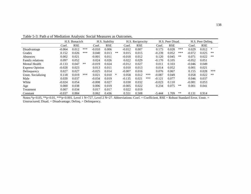
138

Table 5-3: Path a of Mediation Analysis: Social Measures as Outcomes.

H.S. Bonacich H.S. Stability H.S. Reciprocity H.S. Peer Disad. H.S. Peer Delinq.

Coef. RSE Coef. RSE Coef. RSE Coef. RSE Coef. RSE

Disadvantage -0.064 0.012 *** -0.010 0.006

-0.012 0.007

0.175 0.028 *** 0.029 0.012 *

Grades 0.152 0.026 *** 0.040 0.013 ** 0.015 0.015

-0.239 0.052 *** -0.072 0.025 **

Absences 0.002 0.021

-0.001 0.011

-0.018 0.012

0.120 0.045 ** 0.071 0.022 **

Family relations 0.097 0.052

0.024 0.026

0.022 0.029

-0.170 0.105

-0.052 0.051

Mental Health -0.133 0.047 ** -0.019 0.024

-0.012 0.027

0.011 0.103

-0.046 0.049

Express Opinion -0.028 0.023

0.013 0.011

0.010 0.013

0.014 0.052

0.001 0.021

Delinquency 0.027 0.027

-0.025 0.014

-0.007 0.016

0.076 0.067

0.155 0.028 ***

Unstr. Socializing 0.118 0.019 *** 0.021 0.010 * 0.058 0.012 *** -0.087 0.049

0.058 0.022 **

Male 0.020 0.037

-0.034 0.019

-0.135 0.021 *** -0.121 0.077

0.046 0.037

White -0.024 0.054

-0.008 0.027

0.030 0.032

-0.023 0.110

-0.081 0.053

Age 0.000 0.038

0.006 0.019

-0.005 0.022

0.234 0.075 ** 0.001 0.041

Treatment 0.007 0.034

0.017 0.017

0.022 0.019

Constant -0.037 0.884 0.062 0.436 0.551 0.508 -5.444 1.709 ** 0.131 0.914

Notes:*p<0.05, **p<0.01, ***p<0.001. Level 1 N=727, Level 2 N=27. Abbreviations: Coef. = Coefficient, RSE = Robust Standard Error, Unstr. =

Unstructured; Disad. = Disadvantage; Delinq. = Delinquency.

139

Table 5-4: Disadvantage Predicting Educational Attainment, with Social Measures as

Mediators.

Without Mediators With Mediators

O.R. Coef. RSE O.R. Coef. RSE % Med.

Disadvantage 0.759 -0.275 0.080 ** 0.806 -0.215 0.089 *

Popularity

2.157 0.769 0.231 ** 18.39 **

Stability

2.466 0.903 0.477

3.34

Reciprocity

0.705 -0.349 0.443

-1.61

Grades 10.950 2.393 0.216 *** 6.449 1.864 0.183 ***

Absences 0.594 -0.521 0.114 *** 0.549 -0.600 0.129 ***

Family relations 1.561 0.446 0.387

1.725 0.545 0.415

Mental Health 0.976 -0.024 0.259

0.918 -0.086 0.271

Express Opinion 0.861 -0.150 0.146

0.857 -0.154 0.147

Delinquency 0.939 -0.063 0.161

0.826 -0.191 0.150

Unstr. Socializing 0.983 -0.017 0.123

0.900 -0.106 0.164

Male 1.081 0.078 0.189

1.067 0.065 0.225

White 0.515 -0.664 0.320 * 0.446 -0.807 0.349 *

Age 0.615 -0.486 0.274

0.617 -0.483 0.278

Treatment 1.026 0.026 0.246

0.942 -0.060 0.252

Constant 2.876 6.665 2.508 6.884

Notes:*p<0.05, **p<0.01, ***p<0.001. Level 1 N=727, Level 2 N=27. Total mediation = 20.13%,

significant at the p<0.01 level. Abbreviations: O.R. = Odds Ratio, Coef. = Coefficient, RSE = Robust

Standard Error, Med. = Mediated, Unstr. = Unstructured.

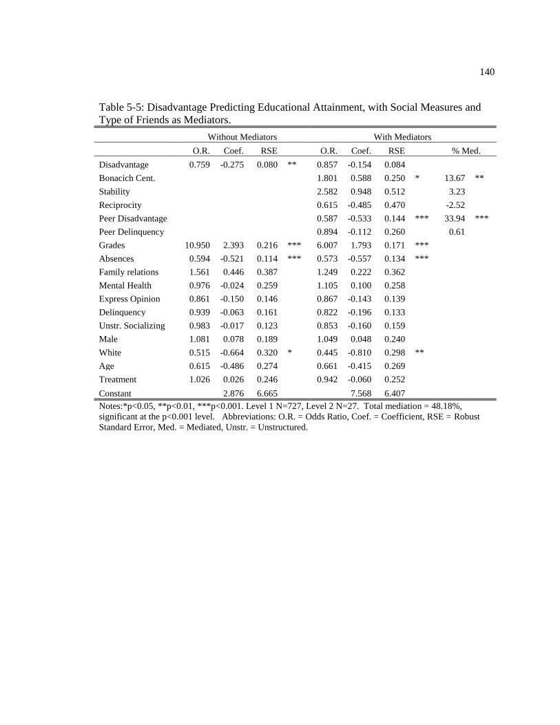
140

Table 5-5: Disadvantage Predicting Educational Attainment, with Social Measures and

Type of Friends as Mediators.

Without Mediators With Mediators

O.R. Coef. RSE O.R. Coef. RSE % Med.

Disadvantage 0.759 -0.275 0.080 ** 0.857 -0.154 0.084

Bonacich Cent.

1.801 0.588 0.250 * 13.67 **

Stability

2.582 0.948 0.512

3.23

Reciprocity

0.615 -0.485 0.470

-2.52

Peer Disadvantage

0.587 -0.533 0.144 *** 33.94 ***

Peer Delinquency

0.894 -0.112 0.260

0.61

Grades 10.950 2.393 0.216 *** 6.007 1.793 0.171 ***

Absences 0.594 -0.521 0.114 *** 0.573 -0.557 0.134 ***

Family relations 1.561 0.446 0.387

1.249 0.222 0.362

Mental Health 0.976 -0.024 0.259

1.105 0.100 0.258

Express Opinion 0.861 -0.150 0.146

0.867 -0.143 0.139

Delinquency 0.939 -0.063 0.161

0.822 -0.196 0.133

Unstr. Socializing 0.983 -0.017 0.123

0.853 -0.160 0.159

Male 1.081 0.078 0.189

1.049 0.048 0.240

White 0.515 -0.664 0.320 * 0.445 -0.810 0.298 **

Age 0.615 -0.486 0.274

0.661 -0.415 0.269

Treatment 1.026 0.026 0.246

0.942 -0.060 0.252

Constant 2.876 6.665 7.568 6.407

Notes:*p<0.05, **p<0.01, ***p<0.001. Level 1 N=727, Level 2 N=27. Total mediation = 48.18%,

significant at the p<0.001 level. Abbreviations: O.R. = Odds Ratio, Coef. = Coefficient, RSE = Robust

Standard Error, Med. = Mediated, Unstr. = Unstructured.

141

Chapter 6

Conclusion

Disadvantage has received much attention within the fields of criminology and

education as scholars have sought to understand why individuals from lower

socioeconomic backgrounds have poorer outcomes (Cohen 1955; Hagan 1992; Coleman

1959). However, the critical aspect of social worlds has not received enough empirical

attention, even though stressed by early leaders like Coleman (1959) and Cohen (1955).

This dissertation examined the indirect effects of disadvantage on adolescent social

relations by using recent, social network data.

This dissertation had two primary objectives: (1) to further our understanding of

the relationship between disadvantage and social success and (2) to examine the

consequences of the relationship between disadvantage and social success. This

dissertation provides evidence that one’s socioeconomic background has effects on

adolescent social success that can be partially explained by specific school, family, and

individual attributes. More specifically, the relationships of disadvantage to students’

school grades, family home condition, and poor mental health results in these factors

playing large mediating roles in the relationships between disadvantage and several

indicators of social success. These mediating effects were evident across all of my

measures of social of social relations, including in-degree, Bonacich centrality, friendship

reciprocity, and friendship stability. Notably, the social relations measures used in this

research are strong because they derive from social network data and other students

142

friendship choices, rather than being limited to respondents’ self-reports. These findings

indicate that there are indeed indirect effects of disadvantage related to adolescent social

relations.

In terms of policy, these findings can benefit social acceptance programs by

helping such programs target individual mechanisms. The findings from this research

imply that academic, family, and other individual characteristics affect adolescent social

relations and, thus, programs attempting to resolve this disparity in social success should

consider a holistic approach across these three dimensions. Further, this research

demonstrates that youth from disadvantaged backgrounds may benefit the most from

such social acceptance programs that target academic, family, and other individual

characteristics.

The second objective of this dissertation was to examine the consequences of the

disparity in social relations for disadvantaged adolescents. This dissertation examined

both short- and long-term consequences of financial disadvantage in adolescence. More

specifically, the findings demonstrated that the structure of adolescent social networks

increases the likelihood that disadvantaged adolescents will have friends who are more

disadvantaged and more delinquent than non-disadvantaged adolescents. Supporting

subcultural theories of delinquency (Cohen 1955), differential association theory

(Sutherland 1947), and researchers from the field of education (Coleman 1959; Wehlage

et al. 1989; Rumberger and Larson 1998), these social disparities have important

consequences for disadvantaged adolescents relative to delinquent involvement and

school instability.

143

Additionally, this dissertation demonstrated that social class stratification in

adolescent popularity has important long-term consequences for educational attainment,

mediating the relationship between disadvantage and attaining a four-year degree.

Combining these findings with prior work that found adolescent popularity to be related

to adult income, disadvantage and adolescent popularity are clearly linked to income and

education in the first few years of the transition to adulthood. Research should continue

to explore the long-term consequences of adolescent social relations. Specifically, future

research should continue to examine how strongly these patterns continue into the

succeeding years as the former adolescents move into full adulthood (e.g. establishing

their careers and families).

Taken together, this dissertation suggests that programs attempting to improve

cohesion in social networks within schools for disadvantaged adolescents should consider

multiple dimensions, both in terms of social relations and causes. In other words, I found

that disadvantage does have an effect on both popularity and qualitative aspects of

friendships. Further, this dissertation improved our understanding of the primary factors

that mediate the relationship between disadvantage and social relations, demonstrating

support that all three (i.e., school, family, and individual) types of factors should be

considered. Additionally, this dissertation demonstrates that adolescent social relations

should be an important focus of research that examines relationships between low

socioeconomic status and short- and long-term consequences.

While this research moves forward knowledge of disadvantage, social relations,

and related outcomes, there are a few limitations worth noting. For one, as discussed

previously, the PROSPER data set was collected from rural to semi-rural communities

144

from Iowa and Pennsylvania that were predominately white. Though this data set had

many features that made it ideal for my current project, the generalizability of my

findings may be lacking. Second, one of the strengths of this data set for my research is

the social network component. However, it should be discussed again that the friendship

choices were restricted to in-school, in-grade friends. This may be a limitation for my

research as subcultural theories of delinquency argue that disadvantaged adolescents may

be especially likely to befriend those in other schools and/or grades, so there is some

question as to how this might be impacting their in-school social ties. However, these

theories predict that these out-of-grade/school friendships should result as adolescents get

older from a lack of in-school social ties. Using data that tracked one’s social ties

beginning in sixth grade through twelfth grade helps to somewhat alleviate this concern.

Additionally, I estimated sensitivity analyses in Chapter 3 that specifically addressed this

out-of-grade and out-of-school friends. Though concerns stemming from this network

bounding are eased based on the results of the sensitivity analyses, this still may be an

important question for future research to address.

In conclusion, my results show the need for continued research on the role of

disadvantage. This dissertation has contributed to both the criminology and education

literatures by examining how one’s social class indirectly affected delinquency, school

instability, and young adulthood adjustment through one’s adolescent social relations.

Finally, this dissertation pointed to promising directions for future research and efforts to

improve the lives of disadvantaged adolescents and young adults.

145

References

Adler, Patricia A., and Peter Adler. 1998. Peer power: Preadolescent culture and

identity. New Brunswick, NJ Rutgers University Press.

Agnew, Robert. 2005. "Why Do Criminals Offend?: A General Theory of Crime and

Delinquency." Los Angeles, CA: Roxbury Publishing Co.

Allen, Joseph P., Joanna Chango, and David Szwedo. 2014. "The adolescent relational

dialectic and the peer roots of adult social functioning." Child

development 85(1):192-204.

Allen, Joseph P., Megan M. Schad, Barbara Oudekerk, and Joanna Chango. 2014. "What

ever happened to the “cool” kids? Long‐term sequelae of early adolescent

pseudomature behavior." Child development 85(5):1866-1880.

Bagwell, Catherine L., Andrew F. Newcomb, and William M. Bukowski. 1998.

"Preadolescent Friendship and Peer Rejection as Predictors of Adult Adjustment."

Child Development 69(1):140-153.

Baillie, Caroline. 2003. “Development in the Disciplines.” Pp. 116-129 in A Guide to

Staff and Educational Development, edited by D. Baume and P. Kahn. Routledge

Baron, Reuben M. and David A. Kenny. 1986. “The Moderator-Mediator Variable

Distinction in Social Psychological Research: Conceptual, Strategic, and

Statistical Considerations.” Journal of Personality and Social Psychology

51(6):1173–82.

Berndt, Thomas J. 1979. “Developmental Changes in Conformity to Peers and Parents.”

Developmental Psychology 15(6):608.

Berndt, Thomas J. 1982. “The Features and Effects of Friendship in Early Adolescence.”

Child Development 53(6):1447-1460.

Berndt, Thomas J. 2002. "Friendship quality and social development." Current directions

in psychological science 11(1): 7-10.

Borgatti, Stephen P., Martin G. Everett, and Jeffrey C. Johnson. 2013. Analyzing Social

Networks. Thousand Oaks, CA: Sage.

146

Bornstein, Marc H., and Robert H. Bradley 2014. Socioeconomic Status, Parenting, and

Child Development. New York, NY: Routledge.

Bowles, Samuel, Gintis Herbert, and Melissa Osborne. 2001. “The Determinants of

Earnings: A Behavioral Approach.” Journal of Economic Literature. 39(4)1137–

1176.

Bradley, Robert H. 2004. "Chaos, culture, and covariance structures: A dynamic systems

view of children's experiences at home." Parenting 4(2-3):243-257.

Bradley, Robert H., Bettye M. Caldwell, and Stephen L. Rock. 1988. "Home

environment and school performance: A ten-year follow-up and examination of

three models of environmental action." Child development 59(4):852-867.

Braithwaite, John. 1981. “The Myth of Social Class and Criminality Reconsidered.”

American Sociological Review 46(1):36-57.

Braxton, John M., Anna V. Shaw Sullivan, and Robert M. Johnson. 1997. "Appraising

Tinto's theory of college student departure." Higher Education-New York-Agathon

Press Incorporated 12:107-164.

John M. Braxton, Jeffrey F. Milem & Anna Shaw Sullivan. 2000. “The Influence of

Active Learning on the College Student Departure Process.” The Journal of

Higher Education 71(5):569-590.

Bronfenbrenner, Urie, and Pamela A. Morris. 2006. “The Bioecological Model of Human

Development.” Pp. 793-828 in Handbook of Child Psychology sixth edition –

Volume 1: Theoretical Models of Human Development, edited by Richard M.

Lerner. Hoboken, NJ: Wiley.

Bukowski, William M., Betsy Hoza, and Michel Boivin. 1994. "Measuring Friendship

Quality during Pre-And Early Adolescence: The Development and Psychometric

Properties of the Friendship Qualities Scale. Journal of Social and Personal

Relationships 11(3):471-484.

Caplan, Gerald. 1974. Support Systems and Community Mental Health: Lectures on

Concept Development. Pasadena, CA, US: Behavioral Publications.

Cassell, John C. 1973. Psychiatric Epidemiology. Pp. 401-410 in American Handbook of

Psychiatry (Vol. 2), edited by G. Caplan. New York: Basic Books.

Cauce, Ana M. 1986. “Social Networks and Social Competence: Exploring the Effects of

Early Adolescent Friendships.” American Journal of Community Psychology

14(6):607-628.

147

Clelland, Donald, and Timothy J. Carter. 1980. “The New Myth of Class and Crime.”

Criminology 18(3):319-336.

Cloward, Richard A. and Lloyd E. Ohlin. 1960. Delinquency and Opportunity: A Theory

of Delinquent Gangs. The Free Press.

Cohen, Albert K. 1955. Delinquent Boys: The Culture of the Gang. The Free Press.

Coie, John D., Dodge, Kenneth A., and Heide Coppotelli. 1982. “Dimensions and Types

of Social Status: A Cross-age Perspective.” Developmental Psychology 18(4):557.

Coleman, James S. 1959. “Academic Achievement and the Structure of Competition.”

Harvard Educational Review 29:330-351.

Coleman, James. 1988. “Social Capital and the Creation of Human Capital.” The

American Journal of Sociology 94:596-20.

Costanzo, Philip R., and Marvin E. Shaw. 1966. “Conformity as a Function of Age

Level.” Child Development 37(4):967-975.

Craft, Anna, Jeffrey, Bob, and Mike Leibling. 2001. Creativity in Education. A&C Black.

Conger, Rand D., Katherine J. Conger, Glen H. Elder, Frederick O. Lorenz, Ronald L.

Simons, and Les B. Whitbeck. 1992. “A Family Process Model of Economic

Hardship and Adjustment of Early Adolescent Boys.” Child Development

63(3):526-541.

Crosnoe, Robert. 2000. “Friendship in Childhood and Adolescence: The Life Course and

New Directions.” Social Psychology Quarterly 63:377-391.

Crosnoe, Robert, Shannon Cavanagh, and Glen H. Elder Jr. 2003. “Adolescent

Friendships as Academic Resources: The Intersection of Friendship, Race, and

School Disadvantage.” Sociological Perspectives 46(3):331-352.

Crosnoe, Robert, and Glen H. Elder Jr. 2002. “Successful Adaptation in the Later Years:

A Life Course Approach to Aging.” Social Psychology Quarterly 65(4):309-328.

Crosnoe, Robert, Rashmita S. Mistry, and Glen H. Elder. 2002. “Economic

Disadvantage, Family Dynamics, and Adolescent Enrollment in Higher

Education.” Journal of Marriage and Family 64(3):690-702.

Csikszentmihalyi, Mihaly, Reed Larson, and Suzanne Prescott. 1977. “The Ecology of

Adolescent Activity and Experience." Journal of Youth and Adolescence

6(3):281-294.

148

Cunha, Flavio, James J. Heckman, Lance Lochner, and Dimitriy V. Masterov. 2006.

“Interpreting the Evidence on Life Cycle Skill Formation.” Handbook of the

Economics of Education 1:697-812.

Davies, Scott. 1999. “Subcultural Explanations and Interpretations of School Deviance.”

Aggression and Violent Behavior 4(2):191-202.

Dean, Alfred, and Nan Lin. 1977. “The Stress-buffering Role of Social Support.” Journal

of Nervous and Mental Disease 165(6):403-417.

Dillman, Don A., Glenn Phelps, Robert Tortora, Karen Swift, Julie Kohrell, Jodi Berck,

and Benjamin L. Messer. 2009. "Response rate and measurement differences in

mixed-mode surveys using mail, telephone, interactive voice response (IVR) and

the Internet." Social science research 38(1): 1-18.

Dumas, Jean E., Jenelle Nissley, Alicia Nordstrom, Emilie Phillips Smith, Ronald J.

Prinz, and Douglas W. Levine. 2005. "Home chaos: Sociodemographic,

parenting, interactional, and child correlates." Journal of Clinical Child and

Adolescent Psychology 34(1):93-104.

Dunaway, R. Gregory, Francis T. Cullen, Velmer S. Burton, and T. David Evans. 2000.

"The Myth of Social Class and Crime Revisited: An Examination of Class and

Adult Criminality." Criminology 38(2):589-632.

Elder Jr, Glen H., Tri Van Nguyen, and Avshalom Caspi. 1985. "Linking Family

Hardship to Children's Lives." Child Development 56(2):361-375.

Elliott, Delbert S., and Suzanne S. Ageton. 1980. “Reconciling Race and Class

Differences in Self-reported and Official Estimates of Delinquency.” American

Sociological Review 45(1):95-110.

Entwisle, Doris R. and Nan Marie Astone. 1994. “Some Practical Guidelines for

Measuring Youth’s Race/ethnicity and Socioeconomic Status.” Child

Development 65(6):1521-1540.

Peggy C. Giordano, Stephen A. Cernkovich, H. Theodore Groat, M. D. Pugh and Steven

P. Swinford. 1998. “The Quality of Adolescent Friendships: Long term

effects?” Journal of Health and Social Behavior 39(1):55-71.

Gottfredson, Michael R., and Travis Hirschi. 1990. A General Theory of Crime. Stanford

University Press.

Grant, Kathryn E., Bruce E. Compas, Alice F. Stuhlmacher, Audrey E. Thurm, Susan D.

McMahon, and Jane A. Halpert. 2003. “Stressors and Child and Adolescent

149

Psychopathology: Moving from Markers to Mechanisms of Risk.” Psychological

Bulletin 129(3):447-466.

Hagan, John. 1997. “Defiance and Despair: Subcultural and Structural Linkages between

Delinquency and Despair in the Life Course.” Social Forces 76(1):119-134.

Hagan, John. 1991. “Destiny and Drift: Subcultural Preferences, Status Attainments, and

the Risks and Rewards of Youth.” American Sociological Review 56(6):567-582.

Hagan, John. 1992. “The Poverty of a Classless Criminology.” Criminology 30:1-20.

Hartup, Willard W. 1996. “The Company They Keep: Friendships and Their

Developmental Significance.” Child Development 67(1):1-13.

Harwell, Michael and Brandon LeBeau. 2010. “Student Eligibility for a Free Lunch as an

SES Measure in Education Research.” Educational Researcher 39(2):120-131.

Hauser, R. M. 1994. “Measuring Socioeconomic Status in Studies of Child

Development.” Child Development 65(6):1541–1545.

Hill, Nancy E., and Stracie A. Craft. 2003. "Parent-school Involvement and School

Performance: Mediated Pathways among Socioeconomically Comparable African

American and Euro-American Families." Journal of Educational Psychology

95(1):74-83.

Hill, Nancy E., and Lorraine C. Taylor. 2004. "Parental School Involvement and

children's Academic Achievement: Pragmatics and Issues." Current Directions in

Psychological Science 13(4):161-164.

Johnson, Anna D., Anne Martin, Jeanne Brooks-Gunn, and Stephen A. Petrill. 2008.

“Order in the House! Associations among Household Chaos, the Home Literacy

Environment, Maternal Reading Ability, and Children’s Early Reading.” Merrill

Palmer Q (Wayne State Univ Press) 54(4):445-472.

Johnson, David W. 1980. “Group Processes: Influences of Student-Student Interaction on

School Outcomes.” Pp. 123-168 in Social Psychology of School Learning, edited

by J. H. McMillan. New York: Academic Press.

Katz, Jack. 1988. Seductions of Crime: Moral and Sensual Attractions in Doing Evil.

New York, NY: Basic Books.

Kith, George D., and Patrick G. Love. 2000. "A cultural perspective on student

departure." Reworking the student departure puzzle 196-212.

150

Kreager, Derek A. 2007. “When it’s Good to be ‘Bad’: Violence and Adolescent Peer

Acceptance.” Criminology 45(4):601-631.

Kreager, Derek A., and Jeremy Staff. 2009. "The sexual double standard and adolescent

peer acceptance." Social psychology quarterly 72(2):143-164.

Kuh, George D., Jillian Kinzie, Jennifer A. Buckley, Brian K. Bridges, and John C.

Hayek. “What Matters to Student Success: A Review of the Literature.”

Commissioned Report for the National Symposium on Postsecondary Student

Success: Spearheading a Dialog on Student Success.

Kwak, Nojin and Barry Radler. 2002. “A comparison between mail and web surveys:

Response pattern, respondent profile, and data quality.” Journal of official

statistics 18(2):257.

Light, John M., and Thomas J. Dishion. 2007. Early Adolescent Antisocial Behavior and

Peer Rejection: A Dynamic Test of a Developmental Process. New Directions for

Child and Adolescent Development 2007(118):77-89.

Lucas, Bill, and Toby Greany. 2000. "Learning to Learn: Setting the Agenda for Schools

in the 21st Century." London: Campaign for Learning.

MacKinnon, David. Introduction to statistical mediation analysis. Routledge, 2012.

McGuire, William J. 1973. "The Yin and Yang of Progress in Social Psychology: Seven

Koan." Journal of Personality and Social Psychology 26(3):446-456.

Merton, Robert K. 1968. Social theory and social structure. New York, NY: The Free

Press Simon and Schuster.

Osgood, D. Wayne, Douglas A. Baals, and Nayan G. Ramirez. “Does free and reduced-

price lunch measure up? A methodological examination of how to measure an

adolescent’s socioeconomic background.” Unpublished.

Osgood, D. Wayne, Barbara J. McMorris, and Maria T. Potenza. 2002. "Analyzing

Multiple-Item Measures of Crime and Deviance I: Item Response Theory

Scaling." Journal of Quantitative Criminology 18(3):267-296.

Parke, Ross D., and Navaz P. Bhavnagri. 1989. "Parents as Managers of Children's Peer

Relationships." Pp. 241-259 in Wiley Series on Personality Processes. Children's

Social Networks and Social Supports, edited by D. Belle. Oxford, England: John

Wiley & Sons.

151

Parker, Jeffrey G., and Steven R. Asher. 1987. "Peer Relations and Later Personal

Adjustment: Are Low-accepted Children at Risk?" Psychological Bulletin

102(3):357-389.

Petrill, Stephen A., Alison Pike, Tom Price, and Robert Plomin. 2004. "Chaos in the

home and socioeconomic status are associated with cognitive development in

early childhood: Environmental mediators identified in a genetic

design." Intelligence 32(5): 445-460.

Piaget, Jean. 1932. The Moral Development of the Child. London: Rutledge and Kegan

Paul.

Raine, Adrian. 1993. Psychopathology of crime. Elsevier Science.

Raudenbush, Stephen W., and Anthony S. Bryk. 2002. Hierarchical Linear Models:

Applications and Data Analysis Methods (Vol. 1). Sage.

Rivera, Mark T., Sara B. Soderstrom, and Brian Uzzi. 2010. "Dynamics of Dyads in

Social Networks: Assortative, Relational, and Proximity Mechanisms." Annual

Review of Sociology 36:91-115.

Rosenthal, Beth Spenciner. 1995. "The influence of social support on school completion

among Haitians." Children & Schools 17(1):30-39.

Rumberger, Russell W., and Katherine A. Larson. 1998. "Student Mobility and the

Increased Risk of High School Dropout." American Journal of Education

107(1):1-35.

Sawyer, Keith. 2017. Group Genius: The Creative Power of Collaboration. Basic Books.

Seltzer, Kimberly, and Tom Bentley. 1999. The Creative Age: Knowledge and Skills for

the New Economy. London: Demos.

Sewell, William H., and Vimal P. Shah. 1967. "Socioeconomic Status, Intelligence, and

the Attainment of Higher Education." Sociology of Education 40(1):1-23.

Shaw, Clifford R., and Henry D. McKay. 1942. Juvenile Delinquency and Urban Areas.

Chicago: University of Chicago Press.

Shi, Ying and James Moody. 2017. “Most Likely to Succeed: Long-Run Popularity

Premium for Adolescents.” Social Currents 4(1):13-33.

Simpkins, Sandra D., David R. Schaefer, Chara D. Price, and Andrea E. Vest. 2013.

"Adolescent Friendships, BMI, and Physical Activity: Untangling Selection and

152

Influence through Longitudinal Social Network Analysis." Journal of Research

on Adolescence 23(3):537-549.

Sirin, Seluck R. 2005. “Socioeconomic Status and Academic Achievement: A Meta-

Analytic Review of Research.” Review of Educational Research 75(3):417-453.

Skahill, Michael P. 2002. "The role of social support network in college persistence

among freshman students." Journal of College Student Retention: Research,

Theory & Practice 4(1):39-52.

Smetana, Judith G., Nicole Campione-Barr, and Aaron Metzger. 2006. "Adolescent

Development in Interpersonal and Societal Contexts." Annual Review of

Psychology 57:255-284.

Spoth, Richard, Cleve Redmond, Chungyeol Shin, Mark Greenberg, Scott Clair, and

Mark Feinberg. 2007. “Substance-use Outcomes at 18 Months Past Baseline: The

PROSPER Community–University Partnership Trial." American Journal of

Preventive Medicine 32(5):395-402.

Staff, Jeremy, and Derek A. Kreager. "Too cool for school? Violence, peer status and

high school dropout." Social Forces87.1 (2008): 445-471.

Starfield, Barbara, Anne W. Riley, Whitney P. Witt, and J. Robertson. 2002. "Social

Class Gradients in Health during Adolescence." Journal of Epidemiology &

Community Health 56(5):354-361.

Steinberg, Laurence. 2007. “Risk Taking in adolescence: New Perspectives from Brain

and Behavioral Science.” Current Directions in Psychological Science 16(2):55-

59.

Sutherland, Edwin H. 1947. Principles of Criminology. Chicago: J.B. Lippincott.

Thomson, Elizabeth, Thomas L. Hanson, and Sara S. McLanahan. 1994. "Family

structure and Child Well-Being: Economic Resources vs. Parental Behaviors."

Social Forces 73(1):221-242.

Tinto, Vincent. 1975. “Dropout from High Education: A theoretical Synthesis of Recent

Research.” Review of Educational Research 45:89-125.

Tinto, Vincent. 1987. Leaving College: Rethinking the Causes and Cures of Student

Attrition. Chicago: University of Chicago Press.

Tinto, Vincent 1987. “Reconstructing the First Year of College.” Planning for High

Education 25(1):1-6.

153

Tinto, Vincent. 1997. “Classroom as Communities: Exploring the Education Character of

Student Persistence.” Journal of High Education 68(6):599-623.

Tittle, Charles R., and Robert F. Meier. 1990. "Specifying the SES/Delinquency

Relationship." Criminology 28(2):271-300.

Tittle, Charles R., Wayne J. Villemez, and Douglas A. Smith. 1978. "The Myth of Social

Class and Criminality: An Empirical Assessment of the Empirical Evidence."

American Sociological Review 43(5):643-656.

Tolonen, Hanna, Satu Helakorpi, Kirsi Talala, Ville Helasoja, Tuija Martelin, and Ritva

Prättälä. "25-year trends and socio-demographic differences in response rates:

Finnish adult health behaviour survey." European journal of epidemiology 21(6):

409-415.

Vaquera, Elizabeth, and Grace Kao. 2008. "Do You Like Me As Much As I Like You?

Friendship Reciprocity and its Effects on School Outcomes among Adolescents."

Social Science Research 37(1):55-72.

Waldrip, Amy M., Kenya T. Malcolm, and Lauri A. Jensen‐Campbell. 2008. "With a

Little Help from Your Friends: The Importance of High‐Quality Friendships on

Early Adolescent Adjustment." Social Development 17(4):832-852.

Warr, Mark. 2002. Companions in crime: The social aspects of criminal conduct.

Cambridge University Press.

Wehlage, Gary G., Robert A. Rutter, Gregory A. Smith, Nancy Lesko and Ricardo R.

Fernandez 1989. Reducing the Risk: Schools as Communities of Support. The

Falmer Press, Taylor & Francis Inc.

Willis, Paul. 1977. Learning to Labour. London: Saxon House.

Wolfgang, Marvin E., and Franco Ferracuti. 1967. The Subculture of Violence: Towards

an Integrated Theory in Criminology. London: Tavistock.

Young, Jacob T.N., J. C. Barnes, Ryan C. Meldrum, Frank M. Weerman. 2011.

“Assessing and Explaining Misperceptions of Peer Delinquency.” Criminology

49(2):599-630.

Youniss, James. 1980. Parents and Peers in Social Development: A Sullivan-Piaget

Perspective. Chicago: University of Chicago Press.

Zhao, Xinshu, John G. Lynch Jr, and Qimei Chen. 2010. "Reconsidering Baron and

Kenny: Myths and Truths about Mediation Analysis." Journal of Consumer

Research 37(2):197-206.

154

VITA

Douglas A. Baals

EDUCATION

2018 Ph.D., Criminology, Pennsylvania State University.

2014 M.S., Criminal Justice, University of North Carolina at Charlotte.

2012 B.A., Criminal Justice, Political Science, University of North Carolina at

Charlotte. Summa Cum Laude.

CONFERENCE PRESENTATIONS

Baals, Douglas A. Subcultures, Delinquency, and Social Relations. Paper presented at

the Annual Meeting of the American Society of Criminology, Philadelphia, PA.

November 2017.

Baals, Douglas A., D. Wayne Osgood, and Nayan Ramirez. Financial Disadvantage,

Popularity, and Delinquency: An Analysis of Longitudinal Social Network Data.

Paper presented at the Annual Meeting of the American Society of Criminology,

New Orleans, LA. November 2016.

Ramirez, Nayan, and Douglas A. Baals. Where You Live and Who You Know:

Community Disadvantage, Peer Group Membership, and Adolescent

Delinquency. Paper presented at the Annual Meeting of the American Society of

Criminology, New Orleans, LA. November 2016.

Sanders, Amber N. and Douglas A. Baals. Exploring the Relationship Between Drinking

Games and Alcohol-Related Consequences: A Test of Competing Hypotheses.

Paper presented at the Annual Meeting of the American Society of Criminology,

New Orleans, LA. November 2016.

Ramirez, Nayan and Douglas A. Baals. Delinquency, Drinking, and Academic Success:

A Test of Subculture Theory. Paper Presented at the Annual Meeting of the

American Sociological Association, Seattle, WA. August 2016.

Baals, Douglas A. and Joseph Kuhns. Gender Differences in Burglary Profiles and

Pathways. Paper presented at the Annual Meeting of the American Society of

Criminology, Washington, D.C. November 2015.

Coston, Charisse and Douglas A. Baals, Amber Sanders, and Anita Blowers. Utilizing

learning communities as a tool for CJ transfer students’ success. Roundtable

presentation at the annual meeting of the American Society of Criminology, San

Francisco, CA. November 2014.