disaster relief supply model for logistic survivability
TRANSCRIPT

DISASTER RELIEF SUPPLY MODEL FOR LOGISTIC
SURVIVABILITYby
Nulee Jeong
A Thesis
Submitted to the Faculty of Purdue University
In Partial Fulfillment of the Requirements for the Degree of
Master of Science
Department of Computer and Information Technology
West Lafayette, Indiana
May 2019
ii
THE PURDUE UNIVERSITY GRADUATE SCHOOL
STATEMENT OF COMMITTEE APPROVAL
Dr. Eric T. Matson, Chair
Department of Computer and Information Technology
Prof. Anthony H. Smith
Department of Computer and Information Technology
Dr. John A. Springer
Department of Computer and Information Technology
Approved by:
Dr. Eric T. Matson
Head of the Graduate Program

iii
Dedicated to God and Family who always be there for me and lead me through the journey

iv
ACKNOWLEDGMENTS
It was honorable journey to study and work with amazing people who guide and
encourage me, with no end. I appreciate my dear committee members, Eric T. Matson,
Anthony H. Smith and John A. Springer who always helped the problem I have with my
research. They were not only my committee member, but also the mentors who give me
the insight and meaning of research which directed me to continue this research in the
right direction. I will not forget all the effort they put on this research together and
sincerely appreciate all the talks we had.
I sincerely appreciate my advisor Eric T. Matson who always listened to my worry
not only on research, but also my future. He is truly my advisor who gives me the strength
to continue what I do and support me in every ways. If were not him, I would have not
been able to start and continue this journey. I will forever appreciate him being my
advisor.
I wants to thank my lab mates and seniors, Yongho, Seongha, Mauricio, Ahmad
Esmaeili, Austin, and Zahra who support me and help me having a more mature
perspective on research. I also thank my friends who give me strength and Eunsuh who
not only support the research, but also helped me enduring the hard time , as a dear friend.
For the last, but not least I dearly appreciate my parents, Maengsuk, and
Younghyun who always support and love me. Whether I fail or succeed, they are always
stand by me and believe in me. Whenever I had hard time with research and life, they wait
for me and raise me from the deepest ground. I acknowledge that every moments could be
possible thanks to my parents.

v
TABLE OF CONTENTS
LIST OF TABLES . . . . . . . . . . . . . . . . . . . . . . . . . . . . . . . . . viii
LIST OF FIGURES . . . . . . . . . . . . . . . . . . . . . . . . . . . . . . . . x
LIST OF ABBREVIATIONS . . . . . . . . . . . . . . . . . . . . . . . . . . . xi
GLOSSARY . . . . . . . . . . . . . . . . . . . . . . . . . . . . . . . . . . . . xii
ABSTRACT . . . . . . . . . . . . . . . . . . . . . . . . . . . . . . . . . . . . xiii
CHAPTER 1. INTRODUCTION . . . . . . . . . . . . . . . . . . . . . . . . . 1
1.1 Background . . . . . . . . . . . . . . . . . . . . . . . . . . . . . . . 1
1.2 Problem Statement . . . . . . . . . . . . . . . . . . . . . . . . . . . . 2
1.3 Scope . . . . . . . . . . . . . . . . . . . . . . . . . . . . . . . . . . 4
1.4 Research Question . . . . . . . . . . . . . . . . . . . . . . . . . . . . 4
1.5 Significance . . . . . . . . . . . . . . . . . . . . . . . . . . . . . . . 5
1.6 Assumptions . . . . . . . . . . . . . . . . . . . . . . . . . . . . . . . 6
1.7 Limitations . . . . . . . . . . . . . . . . . . . . . . . . . . . . . . . . 7
1.8 Delimitations . . . . . . . . . . . . . . . . . . . . . . . . . . . . . . . 8
1.9 Summary . . . . . . . . . . . . . . . . . . . . . . . . . . . . . . . . . 8
CHAPTER 2. REVIEW OF LITERATURE . . . . . . . . . . . . . . . . . . . . 9
2.1 Humanitarian Logistics . . . . . . . . . . . . . . . . . . . . . . . . . 9
2.2 Agent Based Model and Simulation . . . . . . . . . . . . . . . . . . . 12
2.3 Survivability . . . . . . . . . . . . . . . . . . . . . . . . . . . . . . . 14
2.4 Summary . . . . . . . . . . . . . . . . . . . . . . . . . . . . . . . . . 17
CHAPTER 3. HUMANITARIAN LOGISTIC MODEL AND SURVIVABILITY . 19
3.1 Survivability . . . . . . . . . . . . . . . . . . . . . . . . . . . . . . . 19
3.2 Humanitarian Logistics’s Agents . . . . . . . . . . . . . . . . . . . . . 22
3.3 Agent Rule . . . . . . . . . . . . . . . . . . . . . . . . . . . . . . . . 27
3.4 Initial Simulation and Result . . . . . . . . . . . . . . . . . . . . . . . 29
3.5 Scenario . . . . . . . . . . . . . . . . . . . . . . . . . . . . . . . . . 29
3.5.1 Case 1. Truck A(Ta) supplying Demand . . . . . . . . . . . . . 29
3.5.1.1 Result . . . . . . . . . . . . . . . . . . . . . . . . . 30

vi
3.5.2 Case 2. Truck B(Tb) supplying Demand . . . . . . . . . . . . . 32
3.5.2.1 Result . . . . . . . . . . . . . . . . . . . . . . . . . 32
3.5.3 Case 3. Helicopter A(Ha) supplying Demand . . . . . . . . . . 35
3.5.3.1 Result . . . . . . . . . . . . . . . . . . . . . . . . . 35
3.5.4 Case 4. Helicopter B(Hb) supplying Demand . . . . . . . . . . 37
3.5.4.1 Result . . . . . . . . . . . . . . . . . . . . . . . . . 37
CHAPTER 4. MODIFIED LAST MILE DISTRIBUTION . . . . . . . . . . . . 41
4.1 Logistic agent . . . . . . . . . . . . . . . . . . . . . . . . . . . . . . 42
4.2 Last mile distribution agent interaction . . . . . . . . . . . . . . . . . . 43
4.3 Modified Agent Rule . . . . . . . . . . . . . . . . . . . . . . . . . . . 44
CHAPTER 5. SIMULATION RESULT . . . . . . . . . . . . . . . . . . . . . . 45
5.1 last mile distribution . . . . . . . . . . . . . . . . . . . . . . . . . . . 46
5.1.1 Allocating with Truck A(Ta) . . . . . . . . . . . . . . . . . . . 46
5.1.2 Allocating with Truck B(Tb) . . . . . . . . . . . . . . . . . . . 49
5.1.3 Allocating with Helicopter A(Ha) . . . . . . . . . . . . . . . . 51
5.1.4 Allocating with Helicopter B(Hb) . . . . . . . . . . . . . . . . 53
5.2 Multiple kinds of logistic agents . . . . . . . . . . . . . . . . . . . . . 56
5.2.1 Allocating Truck A(Ta) and Truck B( Tb) . . . . . . . . . . . . 57
5.2.2 Allocating Truck A(Ta) and Helicopter A( Ha) . . . . . . . . . . 58
5.2.3 Allocating Truck A(Ta) and Helicopter B(Hb) . . . . . . . . . . 59
5.2.4 Allocating Truck B(Tb) and Helicopter A(Ha) . . . . . . . . . . 60
5.2.5 Allocating Truck B(Tb) and Helicopter B(Hb) . . . . . . . . . . 61
5.2.6 Allocating Helicopter A(Ha) and Helicopter B(Hb) . . . . . . . 62
5.2.7 Expanding logistic agents types . . . . . . . . . . . . . . . . . 63
CHAPTER 6. CONCLUSION AND FUTURE WORK . . . . . . . . . . . . . . 67
6.1 Conclusion . . . . . . . . . . . . . . . . . . . . . . . . . . . . . . . . 67
6.2 Future Work . . . . . . . . . . . . . . . . . . . . . . . . . . . . . . . 71
REFERENCES . . . . . . . . . . . . . . . . . . . . . . . . . . . . . . . . . . 73
APPENDIX A. 2 TYPES OF LOGISTIC AGENT : TRUCK A AND TRUCK B . 81

vii
APPENDIX B. 2 TYPES OF LOGISTIC AGENT : TRUCK A AND HELICOPTER
A . . . . . . . . . . . . . . . . . . . . . . . . . . . . . . . . . . . . . . . . 83
APPENDIX C. 2 TYPES OF LOGISTIC AGENT : TRUCK A AND HELICOPTER
B . . . . . . . . . . . . . . . . . . . . . . . . . . . . . . . . . . . . . . . . 87
APPENDIX D. 2 TYPES OF LOGISTIC AGENT : TRUCK B AND HELICOPTER
A . . . . . . . . . . . . . . . . . . . . . . . . . . . . . . . . . . . . . . . . 93
APPENDIX E. 2 TYPES OF LOGISTIC AGENT : TRUCK B AND HELICOPTER
B . . . . . . . . . . . . . . . . . . . . . . . . . . . . . . . . . . . . . . . . 96
APPENDIX F. 2 TYPES OF LOGISTIC AGENT : HELICOPTER A AND HELICOPTER
B . . . . . . . . . . . . . . . . . . . . . . . . . . . . . . . . . . . . . . . . 101
APPENDIX G. 3 TYPES OF LOGISTIC AGENT . . . . . . . . . . . . . . . . . 113
APPENDIX H. 4 TYPES OF LOGISTIC AGENT . . . . . . . . . . . . . . . . . 119

viii
LIST OF TABLES
3.1 Last mile Logistic Agent’s Capacity . . . . . . . . . . . . . . . . . . . . . 23
3.2 Truck A(Ta)’s last mile distribution to Demand . . . . . . . . . . . . . . . 30
3.3 Truck B(Tb)’s last mile distribution to Demand . . . . . . . . . . . . . . . . 32
3.4 Helicopter A(Ha)’s last mile distribution to Demand . . . . . . . . . . . . . 35
3.5 Helicopter B(Hb)’s last mile distribution to Demand . . . . . . . . . . . . . 37
4.1 Modified Last mile Logistic Agent’s Capacity . . . . . . . . . . . . . . . . 42
5.1 Last mile distribution situation . . . . . . . . . . . . . . . . . . . . . . . . 46
5.2 Extreme Logistic Survivability cases with Truck A(Ta) and Truck B(Tb) . . . 57
5.3 Extreme Logistic Survivability cases with Truck A(Ta) and Helicopter A(Ha) 58
5.4 Extreme Logistic Survivability cases with Truck A(Ta) and Helicopter B(Hb) 59
5.5 Extreme Logistic Survivability Cases with Truck B(Tb) and Helicopter A(Ha) 60
5.6 Extreme Logistic Survivability Cases with Truck B(Tb) and Helicopter B(Hb) 61
5.7 Extreme Logistic Survivability Cases with Helicopter A(Ha) and Helicopter
B(Hb) . . . . . . . . . . . . . . . . . . . . . . . . . . . . . . . . . . . . 62
5.8 Extreme Logistic Survivability with Truck B(Tb), Helicopter A(Ha) and Helicopter
B(Hb) . . . . . . . . . . . . . . . . . . . . . . . . . . . . . . . . . . . . 63
5.9 Extreme Logistic Survivability with Truck A(Ta), Helicopter A(Ha) and Helicopter
B(Hb) . . . . . . . . . . . . . . . . . . . . . . . . . . . . . . . . . . . . 64
5.10 Extreme Logistic Survivability with Truck A(Ta), Truck B(Tb) and Helicopter
B(Hb) . . . . . . . . . . . . . . . . . . . . . . . . . . . . . . . . . . . . 64
5.11 Extreme Logistic Survivability with Truck A(Ta), Truck B(Tb) and Helicopter
A(Ha) . . . . . . . . . . . . . . . . . . . . . . . . . . . . . . . . . . . . 65
5.12 Extreme Cases of last mile distribution to Demand with all logistic agents . . 66
6.1 Summary of Logistics Survivability Bast Cases - Two Logistic Agent Type
Organization . . . . . . . . . . . . . . . . . . . . . . . . . . . . . . . . . 69
6.2 Summary of Logistics Survivability Bast Cases - Organization with 10 logistic
agents . . . . . . . . . . . . . . . . . . . . . . . . . . . . . . . . . . . . 70
A.1 Logistics Survivability with Truck A and Truck B . . . . . . . . . . . . . . 81
ix
B.1 Logistics Survivability with Truck A and Helicopter A . . . . . . . . . . . 83
C.1 Logistics Survivability with Truck A and Helicopter B . . . . . . . . . . . . 87
D.1 Logistics Survivability with Truck B and Helicopter A . . . . . . . . . . . . 93
E.1 Logistics Survivability with Truck B and Helicopter B . . . . . . . . . . . . 96
F.1 Logistics Survivability with Helicopter A and Helicopter B . . . . . . . . . 101
G.1 3 Types of Logistic agent combinations when LDC allows 10 agents . . . . 113
H.1 4 Types of Logistic agent combinations when LDC allows 10 agents . . . . 119
x
LIST OF FIGURES
1.1 Phillippines sign for requesting water after typoon Haiyan [6] . . . . . . . 3
1.2 Relief aids for Hurricane Maria stacked at the port [16] . . . . . . . . . . . 6
3.1 Humanitarian Logistic Agent’s Capacity Loss . . . . . . . . . . . . . . . . 20
3.2 Threshold for Survivability . . . . . . . . . . . . . . . . . . . . . . . . . . 20
3.3 Survivability in Open environment . . . . . . . . . . . . . . . . . . . . . . 21
3.4 Survivability in Closed environment . . . . . . . . . . . . . . . . . . . . . 22
3.5 Agent Interaction in Last mile distribution model for Humanitarian Logistic 24
3.6 Logistic Agent Description for Humanitarian Logistic . . . . . . . . . . . . 25
3.7 Truck A(Ta) assigned to Demand . . . . . . . . . . . . . . . . . . . . . . 31
3.8 Distribution Survivability with Truck A(Ta)’s adjusted capacity . . . . . . . 32
3.9 Truck B(Tb) assigned to Demand . . . . . . . . . . . . . . . . . . . . . . . 33
3.10 Distribution Survivability with Truck B(Tb)’s adjusted capacity . . . . . . . 34
3.11 Helicopter A(Ha) assigned to Demand . . . . . . . . . . . . . . . . . . . . 36
3.12 Distribution Survivability with Helicopter A(Ha)’s adjusted capacity . . . . 37
3.13 Helicopter B(Hb) assigned to Demand . . . . . . . . . . . . . . . . . . . . 39
3.14 Distribution Survivability with Helicopter B(Hb)’s adjusted capacity . . . . 40
5.1 Last mile distribution situation . . . . . . . . . . . . . . . . . . . . . . . . 45
5.2 Truck A(Ta) Organization’s last mile distribution . . . . . . . . . . . . . . 47
5.3 Truck B(Tb) Organization’s last mile distribution . . . . . . . . . . . . . . 50
5.4 Helicopter A(Ha) Organization’s last mile distribution . . . . . . . . . . . . 52
5.5 Helicopter B(Hb) Organization’s last mile distribution . . . . . . . . . . . . 54

xi
LIST OF ABBREVIATIONS
LDC Local Distribution Center
t ton
ICRC International Committee of the Red Cross
WVI World Vision International
WFP World Food Programme
IFRC International Federation of Red cross and Red Crescent Societies

xii
GLOSSARY
Local Distribution Center – Warehouse where the stock of items are stored and distributed
from.
Last mile distribution – The last stage of supply which transporting items from hub to the
final destination.
Survivability – A capability of achieving its original and fundamental goal while the
activities originally required to reach the goal are experiencing hardship from
environments.
Logistic Agent – An entity involved in operation regarding logistics such as transportation
vehicle, driver, and pilots.

xiii
ABSTRACT
Author: Jeong, Nulee. M.S.Institution: Purdue UniversityDegree Received: May 2019Title: Disaster Relief Supply Model for Logistic SurvivabilityMajor Professor: Eric T. Matson
Disasters especially from natural phenomena are inevitable. The affected areas
recover from the aftermath of a natural disaster with the support from various agents
participating in humanitarian operations. There are several domains of the operation, and
distributing relief aids is one. For distribution, satisfying the demand for relief aid is
important since the condition of the environment is unfavorable to affected people and
resources needed for the victim’s life are scarce. However, it becomes problematic when
the logistic agents believed to be work properly fail to deliver the emergency goods
because of the capacity loss induced from the environment after disasters. This study was
proposed to address the problem of logistic agents’ unexpected incapacity which hinders
scheduled distribution. The decrease in a logistic agent’s supply capability delays
achieving the goal of supplying required relief goods to the affected people which further
endangers them. Regarding the stated problem, this study explored the importance of
setting the profile of logistic agents that can survive for certain duration of times.
Therefore, this research defines the “survivability” and the profile of logistic agents for
surviving the last mile distribution through agent based modeling and simulation. Through
simulations, this study uncovered that the logistic exercise could gain survivability with
the certain number and organization of logistic agents. Proper formation of organization
establish the logistics’ survivability, but excessive size can threaten the survivability.
1
CHAPTER 1. INTRODUCTION
This study inquires into the question of last mile distribution’s survivability gained
from the number of allocated logistic agents for achieving the humanitarian logistic
agents’ goal of delivering relief goods. This happens over a specific duration in the
situation where logistic agents survivability is in question are not survivable due to
vulnerabilities acting in the dynamic environment. It introduces this research by
presenting a background on humanitarian logistic agents’ vulnerability on dynamic
situations from a disaster. It also covers the research significance, assumptions, limitation
and delimitations which define the extent of this study.
1.1 Background
There is no universally accepted single definition of disaster. Many studies and
organizations define disasters differently [1]. The United Nations Office for Disaster Risk
Reduction(UNISDR)’s a definition of disasters as follows [2]:
A serious disruption of the functioning of a community or a society at any
scale due to hazardous events interacting with conditions of exposure,
vulnerability, and capacity, leading to one or more of the following: human,
material, economic and environmental losses and impacts.
There are various types of disasters which occur in the world, and the most frequently
occurring natural disaster is flooding which represents 43.4% of the total number of
reported disasters from 1998 to 2017 [3]. After flooding, storms were the second most
frequent disaster type, and earthquakes are third. Regardless of their sizes, location, and
types, natural disasters bring destructive impacts to individuals and overall society.
According to the report, disasters killed 1.3 million people killed and damaged two trillion
dollars(USD) of assets from 1992 to 2012 [4].

2
Against the catastrophic result that disasters cause, disaster management is trying
to mitigate the damage by covering the preparedness, response, and recovery. Although
there are efforts on optimizing disaster management, they still face challenges since the
uncertainty in environments is magnified due to the circumstances in reality. The
humanitarian logistic which regards supplying the essential relief aids to affected people’s
survival is one of the operations which are largely troubled by the dynamic and dangerous
environment. In humanitarian operations, even though the relief aids are successfully
procured, the affected people’s lives are put into danger as the essential goods could not be
reached them. The circumstances which are unfavorable to maintaining the good
condition of logistic agents may reduce the lifespan of logistic agents such as vehicle
malfunction and battery drain, and it challenges the survivability of disaster relief
logistics. Survivability, in this case, means that the original goal of agents is reached even
in the situation where agents cannot do the scheduled task which is fundamentally
required for reaching the goal. Survivability is critically vital in regards to humanitarian
operations because if last mile distribution cannot take place, due to the failure of logistic
agents, it will adversely affect people.
1.2 Problem Statement
The problem addressed by this study is the logistic agents’ unexpected incapacity
to perform the delivery operation at the last mile distribution stage which hinders ultimate
disaster recovery but is rarely considered. Last mile distribution is the final stage which
concerns the delivery from the Local Distribution Centers(LDC) where large amounts of
relief goods to affected areas where demands exist, are stored [5].
For response and recovery after disasters, supplying the relief goods continuously
to the location where the demand exists is critically important. In the situation where the
essentials for living such as water, food, and medicine are scarce, delivering those to the
affected people is crucial for their survival. In the typhoon Haiyan, which hit the
Philippines in 2013, people suffered more from the shortage of relief aids such as food,
water, and medicine because of delayed delivery [7]. Therefore, they did not have a choice

3
Figure 1.1. Phillippines sign for requesting water after typoon Haiyan [6]
other than drinking unclean water from polluted wells which put them into more danger.
The primary reason for this delay was that the logistic agents involved in delivering relief
goods were not available in scheduled operation [8]. The destruction of logistic
infrastructures such as bridges and roads is what makes the transportation agent
unavailable, and this was pointed out for the last mile failure from studies [5] [9] [10].
On top of infrastructure problems, the availability of logistic agents which are
essential for moving relief aids to areas such as trucks and helicopters, are significantly
influential to the success of last mile distribution. If logistic agents are unavailable, the last
mile distribution can fail even with reliable infrastructure. The problem is the logistic
agents who take a significant role in last mile distribution but are susceptible to the
dynamic environment the disaster made at the same time. The harsh environment from a
natural disaster can make the vehicle break down such as punctured tires and engine
failure. Previous research on disaster relief supply rarely considered the possibility of
those agents’ inability to perform their role [5] in the future even though logistic agents
cannot survive infinitely. Since the incapacity of expected agents can result in the delay in
supply [11], the last mile distribution should acknowledge the problem of the situation
where the logistic agents could not deliver the goods at some point and address the
problem with the logistic agent’s assignment with the proper consideration on their
4
vulnerability. Allocating excessive logistic agents into demands where supply should
survive only for a few months will be a waste of resources or capital, since excessive
logistic agents could have been used for other things such as procuring relief aids and
shelters. On the other hand, assigning small numbers of logistic agents to the last mile
distribution operation which should survive, for the long term, will create problems in the
future with unexpected incapacity endangering affected people, like the case of
Haiyan [8].
1.3 Scope
Several things are required for successful humanitarian logistic such as donation,
procurement, inventory checking, and route decision. This study focuses on the logistic
agents’ last mile distribution for the humanitarian logistic. The agent is the entity that
perceives the environment through the sensors and affects the environment through the
actuators [12]. Various agents can be involved in this operation such as donor agent,
government agent, NGO agent, and logistic agent [13]. Since the problem this study
identifies is on the site where actual logistics occur, the study focuses only on agents that
directly contribute to allocating relief aids to the affected area such as demand agent,
allocation agent, and logistic agent. Also, the relief aids that will be delivered during the
operation for this study are also scoped to be water and canned food which do not get
contaminated from the weather condition and consumed daily for survival.
1.4 Research Question
This research contributes answers for following questions:
• Which organization of logistic agents is required for optimizing the last mile
distribution after a disaster for duration of time and the survival?
5
1.5 Significance
As have seen from the previous events such as earthquakes that happened in Haiti
and Japan, disasters bring out the chaos in local society and sometimes globally [14]. For
society to stabilize, not only relief items that are required for people’s wellness, but also
further resources to reconstruct the destroyed infrastructure. The duration that the relief
aids should be delivered for affected people depends on the severity and magnitude of
damage inflicted from disasters. As the last mile distribution’s logistic takes the second
largest portion of the expense for the humanitarian aids organizations next to the staff
cost [15], it is important for them to take a wise decision on logistic agents which can
survive logistics for the specific duration needed to served for areas and at the same time
efficient. As the expense it takes for assigning logistic agents can be instead allocated to
procuring the items that needed to recover, profiling of logistic agents organization that
can survive the last mile distribution is essential. Therefore, this study that tries to
establish the model on distributing resources to affected areas and get the profile of
logistic agents that makes the specific duration of last mile distribution survives with the
consideration on logistic agent’s incapacity to supply in the future is significantly
important. Especially, this study puts the focus on the survivability of last mile
distribution. Last mile distribution is the stage that takes the crucial roles in finally
meeting the demand from affected people by directly supplying items, but has significant
uncertainty.
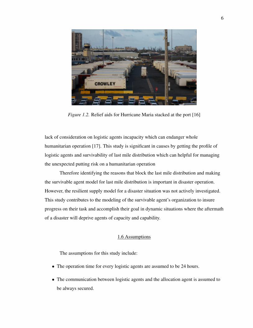
In 2017, Puerto Rico severely suffered from Hurricane Maria. Even though
support had arrived, the relief aids loaded container could not be distributed to the affected
area. According to Crowley, who shipped the 3400 containers at one port in the island,
they unloaded the shipment quickly, but the shipment stayed at the port without quickly
moving to the affected area [16]. Although the support gathered quickly and procurement
was effectively done, the eventual delay at the last mile distribution stage of the
humanitarian supply threatened people’s lives. Studies regard on last mile distribution
6
Figure 1.2. Relief aids for Hurricane Maria stacked at the port [16]
lack of consideration on logistic agents incapacity which can endanger whole
humanitarian operation [17]. This study is significant in causes by getting the profile of
logistic agents and survivability of last mile distribution which can helpful for managing
the unexpected putting risk on a humanitarian operation
Therefore identifying the reasons that block the last mile distribution and making
the survivable agent model for last mile distribution is important in disaster operation.
However, the resilient supply model for a disaster situation was not actively investigated.
This study contributes to the modeling of the survivable agent’s organization to insure
progress on their task and accomplish their goal in dynamic situations where the aftermath
of a disaster will deprive agents of capacity and capability.
1.6 Assumptions
The assumptions for this study include:
• The operation time for every logistic agents are assumed to be 24 hours.
• The communication between logistic agents and the allocation agent is assumed to
be always secured.

7
• The agents’ loading capacity for the operation can be less than maximum.
• Once a logistic agent is assigned to the demand areas, an allocation agent believes
that the logistic agent will deliver the relief aids.
• The route from LDC to each demand area is one unit.
• The decision is made by the allocation agent alone, therefore it is assumed that the
logistic agents always follow the allocation agent’s assignment on the delivery.
• It is assumed that the multiple logistic agents go at the same time using one road is
possible.
• When the agent fails to deliver the goods on the operation for a known or unknown
reason, the situation will be conveyed to allocation agents to decide further action.
• This study assumes that the logistic agents employed at the operation will be new.
• This study assumes that the environment the logistic agents are working can damage
logistic agent but not to the extent of immediate removal.
• Logistic agent’s capacity is expected to decrease gradually because of continuous
operations.
1.7 Limitations
The limitations for this study include:
• The survey data from the previous studies that this study takes into account for
designing agents can be restricted to certain disaster circumstance.
• The study does not take into account the situation where the road is completely
disconnected or can not accommodate the logistic agents for routing.
• Maintenance on logistic agents is not considered in this study.

8
• Logistic agents entails a set of vehicles and one driver or one pilot.
1.8 Delimitations
The delimitations for this study include:
• This study focuses only on the last mile distribution problem among the supply
chain problems in humanitarian operations.
• The study focuses on the last mile distribution, therefore the logistic operation prior
to the Local Distribution Center will not be dealt in the study.
• The study focus on solving the problem with the existing route, therefore, a new
routine decision will not be discussed in this study.
1.9 Summary
This chapter provided the scope, significance, assumptions, limitations, and
delimitations that this study has for the research question asking “Which organization of
logistic agents is required for optimizing the last mile distribution after a disaster for
duration of time and the survival?”. The next chapter provides a review of the literature
relevant to “Disaster Relief Supply Model against Agents Unexpected Incapacity”
including disaster supply, survivability, and agent-based model.

9
CHAPTER 2. REVIEW OF LITERATURE
This chapter provides a review of the literature relevant to the problem of
Humanitarian logistics, the agent based model, and survivability.
2.1 Humanitarian Logistics
For managing disasters, human, capital, and physical resources are put into many
phases such as rescue, evacuation, shelter and restore. Since those resources are limited
but in high demand, managing resources is important for successful disaster management.
Consequently, there is great emphasis on humanitarian logistics. Humanitarian logistics is
the process of planning and controlling the flow and storage of relief aid efficiently from
the support origin to the affected area to alleviate the suffering of victims [18]. This
process covers preparedness, planning, procurement, warehousing, and transport.
Wassenhove claimed that about 80% of disaster relief is about logistics so that the
management on supply should be productive, transparent and precise [19].
Humanitarian relief aid organizations from various sectors provide the general
humanitarian logistic operation once the disaster occurs. When stakeholders on disaster
management acknowledge the disaster, the assessment on the damaged area is initiated to
procure relief aid. In the situation where the limited resources should be efficiently
supplied to many areas, the accurate assessment on the damage is important. Sheu [20]
also said that the task of identifying the right amount of relief goods required for the
affected people is challenging. As Sheu pointed out, the predicted amount of demand for
relief aid might be accelerated due to the circumstance in which people want to secure
more resources for their safety. It can jeopardize overall logistics and put hazard on other
areas suffering from disasters. Regarding this problem, Bendea et al. proposed using
UAVs for gathering the data to support humanitarian operations [21]. They claimed that
satellite images have a limitation because of their instant availability. Instead, they expect
the availability of the relevant data, such as affected areas and the estimated number of
victims from images taken by the camera loaded on autonomously navigating UAVs.
10
Once the assessment on demand is finalized, procuring relief aid based on assessed
needs follows. For this, humanitarian organizations need financial support which can be
established by funding from donors. Donors include government agencies who
traditionally supply the substantial portion of funds, and private donors such as
individuals, trusts, and corporations [22]. Private sectors have come to play a significant
role as donors as their portion of assistance continuously increase. In 2015, it reached the
value of 6.9 billion US dollars approximately. Also, combined support from both sectors
steadily has grown and stretched to 27.3 billion US dollars in 2017 [23]. As the donors
and their influence for humanitarian relief expanded, the need for humanitarian agents to
actually deliver the relief aid by using the funds efficiently and transparently became
important.
About $50 billion US dollars are used on procurement of services and goods for
humanitarian operations. Especially, about 60 percent of the relief aid fund is used on
procuring the relief goods [24]. Even though the primary goods for the relief purpose are
relatively simple, price and availability become the concern when it comes to
humanitarian logistics. Therefore, the procurement process for relief goods should be
considered both locally and internationally depends on situations. The local procurement
has its advantage on transportation time and cost, but international procurement stands out
from the perspective of a large quantity, and low price [25]. Falasca et al. suggested a
two-stage decision model to improve the effective procurement [25]. The model aims to
secure the goods at the first stage despite the uncertainty in need assessment since the act
of supplying upon the disaster is essential. At the second stage in which demand and
donation become relatively sure, the humanitarian organization makes up the gap between
the first stage procurement and the second stage’s assessment so that overall procurement
covers actual demands.
11
After procuring the relief aid locally and globally, relief goods from various
locations arrive at the primary hub in which large transportation such as airplane and the
large ship can be accommodated. Then the supplies go to consecutive warehouses for the
storage and sorting [5]. Those warehouses should be able to cover affected areas because
the number, location, and capacity of warehouses have a significant role in the effective
time and cost management for disaster response [26].
From the warehouse, where a large number of relief aid is stocked, to affected
areas, logistic agents take on a significant role in last mile distribution which is the final
stage of humanitarian logistics [5]. Regarding the operation, the decision for relief aid
allocation, delivery schedule, and routing should be made. However, the problem arises in
reality from the perspectives of limited available transportation, emergency supplies,
damaged road, and coordination problem within humanitarian agents. For this matter,
Balcik et al. proposed the two-phase model on inventory allocation and vehicle schedule
decision in last mile distribution with the consideration of delivery time, vehicle capacity,
and supplying relief aid [5].
Battini et al. got motivation from Balcik et al. [5] and applied the two models to
the Haitian case [15]. This study aims to see the potential of using different transportation
methods such as helicopters, trucks, and a combination of those. From the study, it was
revealed that the costs occurring during the last mile distribution have a higher level of
effectiveness when the different relief aid delivered using the co-transportation.
Ferrer et al. suggested a multi-criteria model for the last mile distribution that
considered not only the traditional criteria such as cost, time, coverage, and equity but also
the security such as the possibility of the ransack happening in the middle of delivery
operation [27].
Majima et al. identified the problem in the logistics’ low robustness in disaster
situation reflecting the previous disaster operations that collapsed due to the damaged
road. The study tries to solve the frail logistics in a disaster environment by using small
ships as alternative [28]. Through the various simulations, the study found the ships’ ideal

12
number, a place to be located. This simulation result can contribute for professionals to
find the place that should be recovered first in case one of the ports used for logistics are
damaged by the disaster. The study shows the survivability feature that the model can
have against the disaster situation which motivates the proposed study.
As Balcik et al. pointed out, the last mile distribution was not fully explored
compared to the other relief logistic problems were studied. Although studies after Balcik
et al’s model modified and applied it to various disaster data, those are more focused on
changing demand in areas. The last mile distribution’s survivability in uncertain
environments after disasters with the organization of logistic agents needs to be studied
2.2 Agent Based Model and Simulation
Agent-based model and simulation is an approach for modeling the dynamic
system of the agents which act autonomously and interact with each other [29]. An agent
is an entity that detects the environment with sensors and changes the environment using
their component [12]. The agents behave upon their rules, interact with other agents, and
cause an impact through those interactions. Based on that, Macal et al. organized the
elements of agent-based model as follows:
• A set of agents, their attributes and behaviors: Agents’ attributes can be static and
dynamic. The static attributes like agent name do not change. On the other hand,
dynamic attributes in the agent such as resource, and capacity can change as they
progress.
• A set of agent relationships and methods of interaction: Agents have dynamic
relationships with other agents and relations further influence agents themselves and
future interactions.
• The agents’ environment: agents also have interaction with the environment. The
interaction entails that agents gather the information from the environment through
the sensor and that they affect the environment.

13
Through the agent-based model, the result that emerged from agents’ dynamic
interactions can be observed and further analyzed. Therefore, it is used for various
research areas such as urban planning, consumer behavior, industrial network, electricity
market and supply chain management [30] [31] [32]. Also, it excels at capturing the
complexity that results from the various interactions between components of society [33]
and this motivates this study to employ agent-based model as humanitarian logistics
especially requires involvement of many agents.
There are studies regards logistics problems and uses agent-based modeling to
solve them. Chen et al. suggested that the crowdsourced delivery would work as the
solution against the challenge they face on last-mile delivery [34]. They modeled
crowdsourcing last mile delivery using an agent-based model to research significant
factors that affect crucial performance in crowdsourcing delivery. They defined three
types of agents; distribution center, package, and crowd carrier. They behave with defined
rules such as crowd carrier identifying the packages that matched to specifications,
picking, and delivering the packages. According to the result from agent-based model
simulations, invaluable findings could be drawn such as that the number of crowd carriers
grows, the detour distance shortens which again increases the benefits of the crowd. For
the problem of delivery capacity shortages in last-mile deliveries, the strategy of giving
incentives to crowds, so they give up the detour time can be drawn. From the simulation,
not only can we gain insight into the phenomenon, the strategy to prevent the problem can
also be experimented.
Chatterjee et al. proposed the public transportation delivery model to prevent
urban areas’ pollution from worsening because of excessive use of private logistic
companies’ transportation [35]. The agents modeled in the proposed system are delivery
agents, bus agents, tram agents, and transport scheduling agents. The delivery agents are
carriers that deliver the package to the designated place. Bus and tram agents are public
transportation agents which carry the delivery agents on each delivery plan. The idea of
agents having the same purpose and function, but different impacts on environment
motivate this study as the logistics could show different results depends on different types
of agents are organized and employed.

14
Fiedrich et al. [36] stressed the potential that the agent technology could be
applied to support disaster management. In terms of the disaster management that should
be executed in a timely and resource-efficient manner, the agent technology can be useful
since it supports intelligent agents to collaborate in a distributed system. The technology
presents the coordination that should be established in the real emergency. In the
circumstance where complex tasks exist and should be executed by different
organizations, using agent technology is expected to help to make decisions about the
coordination problem.
2.3 Survivability
Survivability is the feature that has come to take an essential part in studies
because the purpose should be achieved even though the system is vulnerable and the
nature of the environment is against its purpose. The definition of survivability varies
upon each study.
However, there is consensus on the definition of survivability; it entails the feature
which delivers the essential services that are needed for achieving the system’s goal, even
in situations in which there are attacks on the system and system failure. The common
clarification of survivability that was first defined by Ellison et al. follows
”Survivability is the capability of a system to fulfill its mission, in a timely
manner, in the presence of attacks, failures or accident” [37]
This study stressed that it is the mission that should be survived ultimately, not the part of
the system. Therefore, the most important feature for the survivability is not keeping the
current system; if modifying and reorganizing the system enables the sustaining of the
fundamental mission, it leads to the survivability.
Ellison et al. also depicted the four main keys which are expected to possess for
the survivability [37]. Firstly, the system should be resistant to the attacks. Warding off
the potential attacks beforehand using the user authentication can be one of the examples.
Also, they should recognize that they are getting attack and how much damage they

15
suffered. Against the attack and damage they got, the system should recover fully or to the
extent of at least delivering the essential services for the mission. For recovering or
maintaining the essential services, the system should alter its behavior and functions.
Even though the self-healing may not be appropriate in this study, changing the behavior
so that essential service can be still carried out can be motivation for the survivability in
our study. Lastly, they suggested that the system should be able to evolve to increase its
resistance against the future attack.
There are studies that brought out the vulnerability problem in the system and tried
to increase the survivable feature in fields. Zuo pointed out the lack of survivability
features in the RFID and suggested the potential survivable RFID system [38]. He also
defined the requirements for a survivable system in three aspects as follows :
• Survivable system has the property which services against the damage exist in the
system
• Survivable system accomplishes the original mission even though there are
interruptions against its function
• Survivable system should provide acceptable functions even though it has damaged
Regarding the requirement suggested by Zuo, our study can be motivated to define
the acceptable degree of a function for logistics to be declared as ‘survived status’.
Cardoso et al. expressed the concern on the vulnerability of the workflow
management system and asserted the need for survivability features in the system since
the system could not fully support its role in the sensitive environment. The study
proposed the way of improving the survivability of the METEOR workflow management
system from four level architectures which are instance, schema, workflow, and
infrastructure level [39]. Those are categorical elements that function in the runtime
environment of the system. The study suggested the solutions for each category and
implemented two modules which are dynamic change and adaption. Each module allows

16
the change of instances in workflow level and handles the generated exception based on
the previous experiences the system dealt with. The feature suggested in this study can not
be applied to our study, but changing the instances can motivate how the logistics in our
study can survive.
Gomez et al. tried to put the survivability feature in a multi-agent system where
the mission of the system is on assisting living [40]. Regarding the challenges that the
system can encounter, three strategies based on social interaction are suggested. The first
is finding the agents that have the same capability as the failed agents’ one. The second
strategy is generating a solution based on the different capabilities from agents. The last
one is a more sophisticated strategy which seeks the solutions that previously generated
from the other agents’ experiences. The first strategy can be considered for increasing the
survivability in our study’s problem. Finding the agents which have the same capability as
the deceased agent can be put into prior consideration for survivability in the situation
where the agent loses its capability.
Vincent et al. asserted that the distributed system can be powerful but at the same
time vulnerable to the deliberate attack from outside and system failure [41]. Therefore,
the study suggests that the distributed system should be flexible, and survivable through
the agent coordination scheme which in this case generalized partial global
planning(GPGP).
Agents in environments share their view for problem-solving and negotiate which
agents will take which task. This can be applied to our study since agents can share the
local information they gathered and central agent can allocate the other agents based on
collected information so that the goal of the model can be achieved regarding the problem
that the agent could not carry the expected task.
Tan et al. said that the complexity from global business environment increased the
vulnerability in the supply chain and proposed two strategies creating resilient supply
chain network [42]. Supply chain network is consist of different types of the node which
are retailer, distribution center, and supplier. For the supply chain network to be
survivable, the supply from the supplier should reach to the retailer. Traditional single
supplier supply chain network was very vulnerable, because when the one supplier goes
17
down, then the whole supply chain network encounter crisis of survival. Therefore, the
suggested survivable supply chain network employ network growth models which retailer
chooses the supplier to be linked. The first strategy, ’Hierarchical Preferential
Attachment’, suggests determining the type of node which should be decided on the ratio
of existing nodes type and attached to nodes with relative importance. The second
strategy, ’Hierarchical Random Attachment’ expect the hub of nodes that has high
connectivity would increase the vulnerability of the overall supply chain network.
Therefore, the strategy makes the nodes to be attached to the upper node randomly and at
the same time distributed uniformly. This does not make the one nodes to become heavy
with lots of connection to retailers. Through the simulation analysis, suggested strategies
are revealed to be much resilient compared to the traditional single supplier supply chain.
From this study, the importance of survivable model for the supply chain could be once
again acknowledged. Also, the models that applied to the situation and the evaluation
could also be applied to our study that aims to increase the survivability of last mile
distribution even though the nodes in the problem would be different.
For the problem this study put significance on, the essential function of agent
organization which carries the task of delivering the relief aid to the final destination
should be maintained for the goal of supply relief aid to be survivable. Therefore, for the
sake of the survival of the ultimate goal, organization transition can happen such as agent
task change, and transfer of task.
2.4 Summary
This chapter provided reviews of the literature to humanitarian logistics,
agent-based model, and survivability which are relevant to “Disaster Relief Supply Model
survivable to Agents Unexpected Incapacity”. Those provide the background knowledge
on humanitarian logistics’ various decision making and its issues. For the proposed study,

18
the literature on agent-based modeling and survivability suggest the fundamental concept
needed for defining the survivability in the problem of this study and motivations that
could be considered on modeling the survivable last mile distribution in humanitarian
logistics.
19
CHAPTER 3. HUMANITARIAN LOGISTIC MODEL AND
SURVIVABILITY
This study aims to solve the problem of humanitarian logistic last mile distribution
endangered by logistic agents’ capacity loss shortening the agent’s survival period. Agents
and their behavior are described in this chapter. Also, the definition of ‘Survivability’ in
the humanitarian logistics’ last mile distribution will be defined.
3.1 Survivability
The definitions on ‘survivability’ depends on the studies, but has the general
agreement on the significance of accomplishing its original and ultimate goal. Even
though threatened by the attack and its error, survivability puts the priority on fulfilling the
overall system’s goal even though sustaining the original behavior is sacrificed. From the
perspective on ‘agent’ concept, therefore, survivability is defined as agents accomplishing
their ultimate goal in the situation where their capability is threatened to be decreased or
lost.
Humanitarian logistic agents in this study have the ultimate goal of satisfying the
affected area’s demand by supplying relief aid. When the end goal of humanitarian
logistic agents is considered, whether the last mile distributions survive or not against the
damages depends on if the requested relief aids can be covered by the logistic agents’ total
capacity. Even though the humanitarian logistic agents lost its capacity or capability
because of the environmental factors, if the loading capacity the logistic agents can deliver
to the affected area exceeds area’s demand, then humanitarian logistic agents’ ultimate
goal is achieved, in other words, survives.
Suppose there are two humanitarian logistic agents work on delivering the relief
aids to one affected area P1 daily. The logistic agents, however, lose their capacity to
deliver a certain amount of essential goods to the affected area day by day because of the
harsh environment, after a disaster like the situation shown at the figure 3.1.

20
Figure 3.1. Humanitarian Logistic Agent’s Capacity Loss
Even though their total capacity decreases, last mile distribution survives because
a logistic agents’ capacity is not zero. However, the last mile distribution fails to achieve
its goal from day 7 since humanitarian logistic agent’s supply becomes insufficient to
satisfy the demand which means failure to the goal and at the same time to survival as can
be seen from Figure 3.2.
Figure 3.2. Threshold for Survivability

21
Therefore, the logistic agents’ last mile distribution goal to be achieved and
survive, the logistic agents’ capacity should be adjusted at least until the point of the
affected area’s demand.
In an open environment, the logistic agents which, were not participating in the
operation, can join and participate in last mile distribution. Figure 3.3 shows the
survivability in an open environment. If the entered logistic agents’ capacity is sufficient
to cover the gap between the demand and overall agents’ capacity, humanitarian logistic
agents could deliver the demanded amount of relief aids to the affected area. Therefore,
the ultimate goal of logistic agents can be achieved, so last mile distribution survives, with
the additional capacity.
Figure 3.3. Survivability in Open environment
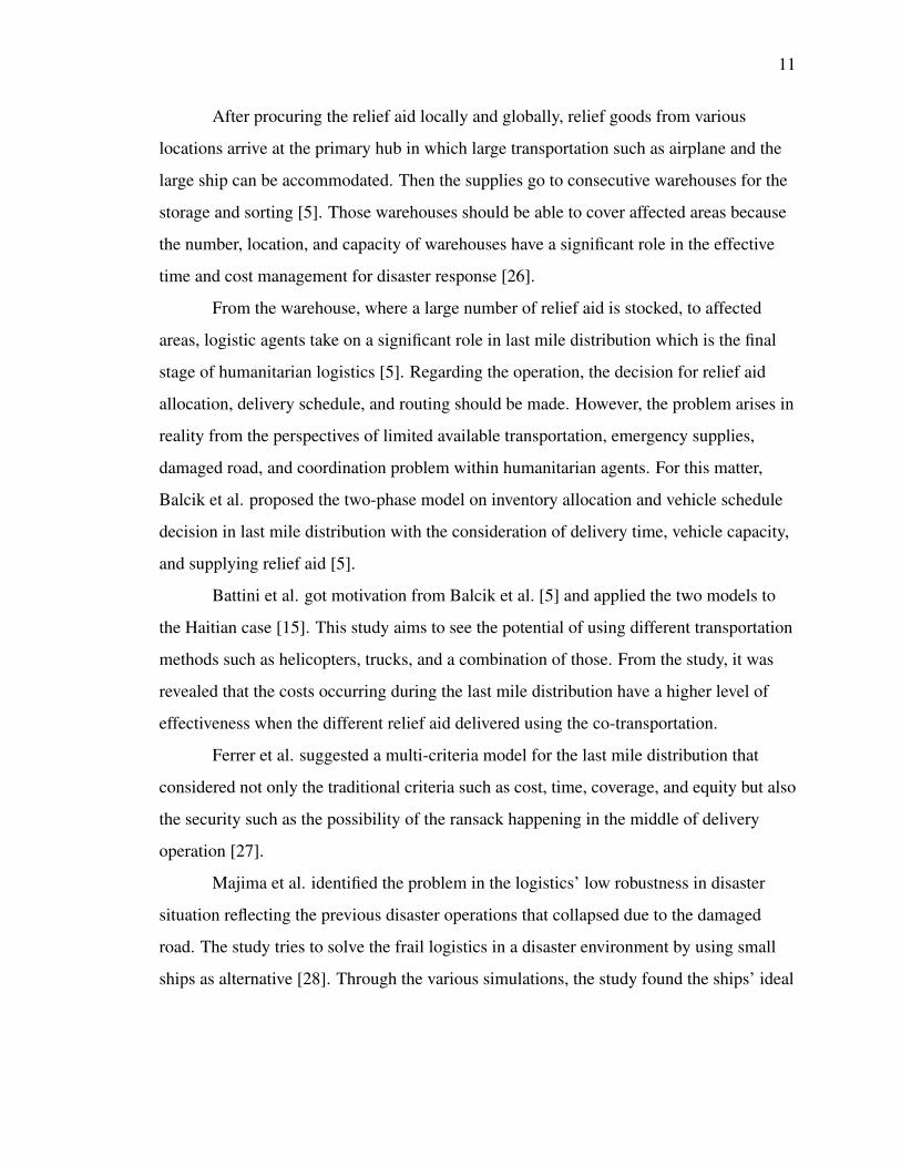
On the other hand, in a closed environment, the additional agents from the outside
of the environment where the current logistic agents are working cannot enter. Figure 3.4
shows the survivability in a closed environment. Therefore, for the humanitarian logistics’
last mile distribution to survive, the allocation agent should coordinate the remaining
logistic agents’ capacity and their assignment to the area, so the adapted capacity from
allocation agent’s coordination can satisfy unmet demand. As the adjusted capacity from
the cooperation is above the minimum level of demand, the logistic agents’ goal comes to
achieved and last mile distribution survives.
22
Figure 3.4. Survivability in Closed environment
Consequently, in the situation where the logistic agents lose their capacity, the
humanitarian logistic’s last mile distribution survives when every area’s demands are
satisfied with the supply that was enabled from the allocation agents’ coordination
decision on logistic agents. Employing logistic agents which survives the last mile
distribution for the duration of time which is needed for the affected areas to recover is
important.
3.2 Humanitarian Logistics’s Agents
The humanitarian logistic’s last mile distribution model has three agents, demand
agents, allocation agents, and logistic agents.
Demand agents are situated at the affected areas, and they put the request for relief
aid to the allocation agent so that the affected area’s victim can be relieved with the relief
aids supply. Demand agents have ‘Need’ and ‘Need’ means the quantity of relief aids that
demand area requires from the local distribution center. The quantity of ‘Need’ is renewed
every day until the end of the operation. The ‘Need’s from demand agents are significantly
important as they are the criteria deciding the success and failure of humanitarian logistic,
and also their survivability.

23
An allocation agent is a central agent located at the LDC which gets the request of
relief aids from the demand agents. This agent pursues the humanitarian logistics’ ultimate
goal of satisfying the demand of the affected area’s victim by supplying relief aids so that
the suffering of affected people can be alleviated. Therefore, they get the request from the
demand agent, assesses the reported availability of logistic agents to satisfy the needs.
Then, the allocation agent allocates the specific amount of relief aids to logistic agents and
assign them the area where they have to deliver the items based on the assessment.
Logistic agents execute the tasks given by the allocation agents which, are
delivering the allocated relief aids to the assigned areas. They load the specific amount of
relief aids and move with the allowed speed at maximum. It takes time to load and unload
the goods depend on the quantity they deliver. After logistic agents arrive and unload the
carried items at the assigned demand area, they return to the LDC to for the further
deliveries or the end of the daily delivery.
Under logistic agents, there are four logistic agent types which reflected the real
logistic transportation used in humanitarian logistics such as the Haitian humanitarian
logistic [43]. There are two ground vehicles which are off-road trucks and two aircraft for
the last mile distribution. Table 3.1 is the description of logistic agents that will be
modeled in this scenario.
They show the difference in their capacity regarding the loading and speed by
logistic agents’ types.
Table 3.1. Last mile Logistic Agent’s Capacity
Ground Vehicle Aircraft
Agent Truck A Truck B Helicopter A Helicopter B
Loading Capacity(tonne) 7.5 14 2.5 2
Operational Speed(km/h) 85 85 180 160

24
Other than loading capacity and speed, the logistic agents have other attributes
such as status, destination, history, sequence, and LDC. Status shows the state where the
logistic agents, are such as located at the LDC, moving to the destination, delivery, and
returning to the LDC. Destination differs by the agent, and it tells where the logistic agent
will deliver its capacity until the needs of the destination are satisfied. Each logistic agent
remembers which demand they visited and its sequence. Then, they repeat it daily until
the end of the operation.
Agents in humanitarian logistics’ last mile distribution model only pursue their
goals of supplying relief goods to the affected areas. Figure 3.5 is the agent interaction
diagram for humanitarian logistics’ last mile distribution models to achieve the goal of
satisfying the requested demand by supplying with relief aids.
Figure 3.5. Agent Interaction in Last mile distribution model for Humanitarian Logistic

25
Figure 3.6 shows the fundamental attribute the logistic agents have to deliver the
task for last mile distribution. When the logistic agent who moves the relief items stored
at the allocation place to demand A is a1, a1 have the capacity of loading, speeding and
operating. The loading capacity, Ca1 is how much weight of relief items a1 can load. The
overall speed, Sa1 shows the how fast a1 can move from allocation place to demand area
A. Finally, general operation time means that the working hour the logistic agent, a1 will
do the task of delivering.
Based on the defined agents above in the humanitarian logistics’ last mile
distribution model, suppose the situation where the agent a1 should deliver a certain
amount of relief aids to the affected area p1 in the last mile for humanitarian logistic.
Figure 3.6. Logistic Agent Description for Humanitarian Logistic
Where the distance from Local Distribution Center(LDC) to the affected area p1 is
dp1, and the agent a1’s speed capacity is sa1, the time taking for agent a1 to arrive at the
affected area p1 is ta1p1.
ta1p1 =dp1
sa1(3.1)
For the logistic agent a1 to complete the task of delivering relief aids to the
affected area, the agent a1 should depart from the LDC and arrive at the affected area p1,
then come back to the LDC. Therefore, it takes 2ta1p1 time for agent a1 to complete one
round of distribution task to p1.

26
Suppose the agent a1 has a certain amount of time h hours that can be operated for
a day. Then, ra1p1 defines how many rounds the agent a1 can transport to the affected area
p1 which can be calculated as below.
ra1p1 =
[h
2 ta1p1
](3.2)
When the loading capacity the logistic agent a1 can perform at one round is ca1,
the entire amount of relief aids that logistic agent a1 carry and distribute to the p1 area can
be expressed as Ca1p1 and calculation follows.
Ca1p1 = ra1p1 ∗Ca1 (3.3)
For logistic agent a1 to accomplish its ultimate goal in the last mile distribution, its
total loading capacity, Ca1p1 should be always equal to or greater than the p1 area’s
demands on relief aids as shown in equation 3.4.
Ca1p1 ≥ Np1 (3.4)
If there are x number of logistic agents and y number of affected areas where the
last mile distribution model has to serve, how many number of agent types are assigned to
where can be expressed with the matrix. When the number of agent a1 assigned to area p1
can be expressed as Na1p1, following matrix can be created.
N =
Na1p1 Na2p1 ... Naxp1
Na1p2 Na2p2 ... Naxp2
... ... ... ...
Na1py Na2py ... Naxpy
Also, the capacity of agent type depends on the area which is expressed with the
matrix P. As defined above, the total quantity of relief aids that logistic agent a1 can carry
and deliver to the p1 area can be expressed as Ca1p1. If so, the total capacity each agent
have for the area can be normalized like below matrix.

27
P =
Ca1p1 Ca1p2 ... Ca1py
Ca2p1 Ca2p2 ... Ca2py
... ... ... ...
CaX p1 CaX p2 ... Caxpy
When both matrices multiplied, the total loading capacity that would be delivered
to a specific area with the N configuration can be calculated like below.
C =
Na1p1 Na2p1 ... Naxp1
Na1p2 Na2p2 ... Naxp2
... ... ... ...
Na1py Na2py ... Naxpy
Ca1p1 Ca1p2 ... Ca1py
Ca2p1 Ca2p2 ... Ca2py
... ... ... ...
CaX p1 CaX p2 ... Caxpy
=
Cp1 ... ... ...
... Cp2 ... ...
... ... ... ...
... ... ... Cpy
From a diagonal line in the matrix C, the total loading capacity that can be
deliverable to each area with the certain configuration of agent types’ number and capacity
can be known. For example, the Cp1 would be the total loading capacity transferred to
area p1 with the agent’s number and capacity assignment from matrix N and P. When
each capacity can cover the demand from each area, the goal of humanitarian logistic is
achieved.
3.3 Agent Rule
Following is the behavior rule of logistic agents in last mile distribution model.
Based on the behavior completion, logistic agents change their status.
Check-destination The logistic agent checks its destination to decide if it will
continue its delivery or not. Logistic agents check the status of destination if it is fulfilled
with the demand. When the need of destination is left unsatisfied and the logistic agent
finished supplying needs posted from demand agent they were initially assigned, they set
up the unsatisfied demand area as new destination randomly.

28
Load Before departing from LDC, the logistic agent should load the relief aids.
The quantity of items that will be loaded depends on allocation agent’s decision. For
loading the items for operation, there are tasks to be done such as reporting, and
preparation equipment to load items. Burdzik et al. studied the time taken for the task of
loading the items [44] and time was reflected to the model. Following equation shows the
time taken for loading task based on the work of Burdizik et al [44].
TL = 67+(LoadingAmount ∗2357)∗0.0000027903(min) (3.5)
Move The logistic agents head to the destination with the speed with which the allocation
agent suggest them to move. The tough environments which are assumed to be the
environment where the logistic agents are working in this study are unfavorable to a
logistic agent’s capability. In this model, logistic agents have their capacity reduced such
as payload and speed. As the damage logistic agents received influences from continuous
operations, logistic agents are limited on their speed and capacity for further delivery.
Unload The actual delivery of relief aid happens once the loaded items are
unloaded from the logistic agents arriving at the destination. Also, unloading items is
necessary as the logistic agents can return to the LDC when they go through the unloading
process. Like loading the item, unloading relief items takes time, so logistic agents should
stay at the destination for a specific duration for the unloading process to be done. The
tasks required for unloading items differ with tasks for loading item, so the time they stay
for unloading can be estimated as below [44].
TUL = 59+(LoadingAmount ∗1861)∗0.0000027903(min) (3.6)
Return The logistic agent returns to LDC after they finish unloading the relief aid
to the destination. Return behavior is needed for agents because the relief aid are stacked
at the LDC, the logistic agent can do further distribution when it comes back the LDC and
load the new relief aid that matched to the needs from destinations.

29
3.4 Initial Simulation and Result
Agent’s rule and behavior were modeled with NetLogo which is well known
multi-agent modeling program [45]. In order to get the optimal profile of a logistic agent
that survive humanitarian logistics, the humanitarian logistic agent model is also
simulated by varying the logistic agents’ capacity initially.
3.5 Scenario
Four cases where different types of logistic agents are delivering relief aids to a
demand area were simulated to get the baseline profile of capacity needed for achieving
the survivability to survive logistic for the duration of time.
As the logistic agent types have different maximum loading capacities or
operational speed, it is expected that capacity loss on agent differs by agent types which
influence each logistic agent type’s survivability for the operation to the demand area.
One demand in this simulation is 79km away from the LDC where the allocation
agent and logistic agents are located. Also where the environment where the last mile
distribution is done from LDC to demand area in below four cases are assumed to be
hazardous to ground vehicle, rather than aircraft. The demand agent at an affected area
requests water containers weighing 6,737kg and needs to supply the water every day as
the water is needed for daily living.
3.5.1 Case 1. Truck A(Ta) supplying Demand
In this case, the baseline is that one truck A being assigned for supplying the
waters to the Demand A speeding at 85km/h when departed and loading 7.5t per one
operation.

30
3.5.1.1 Result
Table 3.2. Truck A(Ta)’s last mile distribution to Demand
Truck A
Number Loading(t) Speed(km/h) Logistic Survival Days
1 7.5 85 2
From the result, the truck A could deliver the required amount of relief aids for
two days with baseline capacity. With baseline capacity, Truck A could finish the
distribution in one round of travel until the end of day 1. However, the damage because of
speed and capacity during continuous operation hinders the truck A to survive after the
second day of operation. Figure 3.7(a) shows the great damage the logistic agent got from
the first travel to the demand. To increase the survivability of truck A’s last mile
distribution, an adjustment on Truck A’s loading and speeding capacity were simulated
further. To make this logistic survivable, truck A’s speed and loading capacity is adjusted
with 836 runs of the simulation. Figure 3.8 is showing the survival days change by
adjustment on capacity and speed.
At the maximum speed which Truck A can move, survival days vary by the
capacity they load. When truck A load items weighing from 6.8t to 7.5t, the logistics can
survive for 2 days. However, when Truck A loads from 2.3t to 6.7t, the truck can survive
for 1 day. The worst case is loading under 2.2t as they need to do 8 rounds of travel to
complete the delivery task. Even though the capacity is less per operation, they need to do
four times more round trips than when they load the maximum amount per each operation,
and it eventually lowers the logistics ’ survivability with Truck A. Survivability with
Truck A can be maximized to 3 days when Truck A moves at 45km/h loading 7.5t of relief
aids per operation.

31
(a) Speeding Capacity Loss
(b) Loading Capacity Loss
(c) Survival Days
Figure 3.7. Truck A(Ta) assigned to Demand

32
Figure 3.8. Distribution Survivability with Truck A(Ta)’s adjusted capacity
3.5.2 Case 2. Truck B(Tb) supplying Demand
In this case, Truck B is assigned for supplying the relief aids to the demand area.
This truck exhibits baseline speeding capacity by moving at 85km/h. Contrary to truck A,
truck B is capable of loading 14 tons of items per one operation. Table 3.3 shows last mile
distribution survivability when truck B distribute with baseline capacity.
3.5.2.1 Result
Table 3.3. Truck B(Tb)’s last mile distribution to Demand
Truck B
Number Loading(t) Speed(km/h) Logistic Survival Days
1 14 85 2

33
(a) Speeding Capacity Loss
(b) Loading Capacity Loss
(c) Survival Days
Figure 3.9. Truck B(Tb) assigned to Demand

34
The round trips Truck B should make for satisfying the demand is one. As baseline
capacity per operation already covers the needs from the Demand A, Truck B can survive
at least one day, but shows dramatic decrease in speed capacity as the operation goes by.
As the loading capacity and speed adjusted for Truck B, the survival days showed
the change. Figure 3.10 is graph showing survival results with the modified capacity .
Figure 3.10. Distribution Survivability with Truck B(Tb)’s adjusted capacity
From the Figure 3.10, loading capacity plays a major role in deciding survival
days can be seen. As the amount of relief aids that Truck B loads get bigger, the survival
days are also shown to be increased. The best case was B type trucks surviving logistics
for three days when its speed is decreased to 45km/h and it loads 13.9 tons of items. On
the other hand, the logistic shows the worst case of non-survival when it loads items under
2.2 tons per operation even truck moved with maximum speed. As the quantity of loaded
items per travel becomes smaller, the round of travel that Truck B should do to deliver all
requested relief items increases and it shortens the time when Truck B can keep its
delivering capability which results in an adverse effect on logistics’ survivability.
35
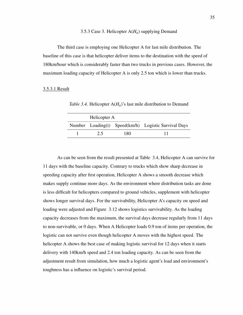
3.5.3 Case 3. Helicopter A(Ha) supplying Demand
The third case is employing one Helicopter A for last mile distribution. The
baseline of this case is that helicopter deliver items to the destination with the speed of
180km/hour which is considerably faster than two trucks in previous cases. However, the
maximum loading capacity of Helicopter A is only 2.5 ton which is lower than trucks.
3.5.3.1 Result
Table 3.4. Helicopter A(Ha)’s last mile distribution to Demand
Helicopter A
Number Loading(t) Speed(km/h) Logistic Survival Days
1 2.5 180 11
As can be seen from the result presented at Table 3.4, Helicopter A can survive for
11 days with the baseline capacity. Contrary to trucks which show sharp decrease in
speeding capacity after first operation, Helicopter A shows a smooth decrease which
makes supply continue more days. As the environment where distribution tasks are done
is less difficult for helicopters compared to ground vehicles, supplement with helicopter
shows longer survival days. For the survivability, Helicopter A’s capacity on speed and
loading were adjusted and Figure 3.12 shows logistics survivability. As the loading
capacity decreases from the maximum, the survival days decrease regularly from 11 days
to non-survivable, or 0 days. When A Helicopter loads 0.9 ton of items per operation, the
logistic can not survive even though helicopter A moves with the highest speed. The
helicopter A shows the best case of making logistic survival for 12 days when it starts
delivery with 140km/h speed and 2.4 ton loading capacity. As can be seen from the
adjustment result from simulation, how much a logistic agent’s load and environment’s
toughness has a influence on logistic’s survival period.

36
(a) Speeding Capacity Loss
(b) Loading Capacity Loss
(c) Survival Days
Figure 3.11. Helicopter A(Ha) assigned to Demand

37
Figure 3.12. Distribution Survivability with Helicopter A(Ha)’s adjusted capacity
3.5.4 Case 4. Helicopter B(Hb) supplying Demand
The last case is when the B type helicopter is assigned to an affected area. B type
helicopter’s baseline capacity in speed is 160km/hour, which is slower than Helicopter A,
but is faster than the trucks. Also, base loading capacity is only 2 tons, and this is less than
A helicopter’s base loading capacity.
3.5.4.1 Result
Table 3.5. Helicopter B(Hb)’s last mile distribution to Demand
Helicopter B
Number Loading(t) Speed(km/h) Logistic Survival Days
1 2 160 7

38
From the baseline simulation, Helicopter B is reported to survive for seven days in
a row. As the loading and speed capacity is lower than A helicopter, B helicopter is shown
to survive logistics less than A helicopters. To increase the survivability of Helicopter B’s
distribution, the loading and speed capacity adjustment were simulated, and survivability
is on following Figure 3.14.
According to the simulation result presented at Figure 3.14, logistic survival days
with Helicopter B shows a decreasing trend as they load less amount of relief aids per
round. This trend accords with results from the cases that employed a different kind of
logistic agents. The logistics with Helicopter B shows the worst survival days when it
loads less than 0.9 tons of items. Even with the maximum speed of 200km/h, the logistic
could not survive when helicopter B loads less than 0.9 ton items per operation.
Regardless of the time that B helicopter can finish the one round of travel, the logistic
agents cannot deliver the total requested items if the time of travel is too large. Helicopter
B shows the best case by keeping logistic alive for 8 days with 130km/h speed and 1.9 ton
loading. Even with the lower than operational speed, helicopter B can make last mile
distribution survivable when loading capacity is big enough.

39
(a) Speeding Capacity Loss
(b) Loading Capacity Loss
(c) Survival Days Loss
Figure 3.13. Helicopter B(Hb) assigned to Demand

40
Figure 3.14. Distribution Survivability with Helicopter B(Hb)’s adjusted capacity

41
CHAPTER 4. MODIFIED LAST MILE DISTRIBUTION
From the simulation with the approach inflicting damage on speed and capacity
every minute, it was found that the approach inflicting damage on logistic agents is
unrealistic as it resulted in 11 days of last mile distribution survival, at most, when logistic
agents move with the reasonable speed and loading specification. Survival longer than 30
days is also found to be with helicopters traveling with 90km/h which is also unreasonable
for the helicopters.
As damage is inflicted on logistic agents, in the model, was deemed to be
inappropriate, the approach how the logistic agents were damaged from the last mile
distribution in this study was adjusted with the new attribute which is the lifespan of
logistic agents. Lifespan means the average age of trucks and helicopters. According
to [46], the truck is revealed to be operable for about 12 years. The helicopter’s average
age was also researched but could not be founded from sources, therefore it was also set to
12 years. Therefore, the model is modified that the logistic agents which travel in an
organized environment such as the even road condition and stable landing space can be
operable for 12 years.
However, the logistic agents in this study do rough operations compared to
vehicles which are used for a daily commute. As can be seen from the simulation results,
the logistic agents acquire damage as they complete more rounds of last mile distribution.
Martinez et al. [47] provided the information on the average age of vehicles
employed on humanitarian logistic. Among four international humanitarian organizations,
ICRC(International Committee of the Red Cross) and WVI(World Vision International)
mobilized vehicles very frequently with the purpose of transporting relief items and
materials for the recovery, which is matched to the goal of last mile distribution. Since
their usage aligns with the last mile distribution, which is the environment and tasks this
study focus on, the average age of vehicles from those organization motivated the damage
on logistic agents by decreasing the lifespan, as they continue operation for the last mile
distribution on disaster environment.

42
Contrary to the damage on logistic agents which is very frequently used for the last
mile distribution, WFP and IFRC used the vehicles rarely or occasionally for last mile
distribution. Therefore, the damage on the lifespan of logistic agents which are used
infrequently for last mile distribution was motivated from fleet age of vehicles belongs to
WFP(World Food Programme) and IFRC(International Federation of Red cross and Red
Crescent Societies).
Apart from the occasion or substantial assignment to last-mile distribution, the
logistic agents also have the danger of sudden incapability when they are idle for the
duration, such as 30 days, with battery drain [48].
4.1 Logistic agent
The specification of the logistic agent in this study take a significant role in this
study as their speed and loading capacity change how many rounds of travel is required to
survive the last mile distribution, and it affects the logistic agent’s non-operation status
thus affecting the survivability of last mile distribution.
Table 4.1 shows the specification of four logistic agents that were used for
modified last mile distribution in this study and this is motivated by the logistic agents
used for operation at Haiti [43].
Table 4.1. Modified Last mile Logistic Agent’s Capacity
Ground Vehicle Aircraft
Agent Truck A Truck B Helicopter A Helicopter B
Loading Capacity(t) 7.5 14 3 2
Maximum Speed(km/h) 105 105 217 205
43
A type truck(Ta) is the Renault truck and it can load 7.5 tons of items [43, 49]. B
type truck(Tb) can load 14 tons, and it is produced by the DAF [43, 50]. For both types of
trucks, the maximum speed is motivated from Hawaii’s driving speed regulation on state
highway [51] as the Haitian’s driving regulation for trucks could not be found and Hawaii
as an island have a similar environment. Helicopter A(Ha) is motivated from Bell 205
which can load 3-4 tons of items from the report, but defined to load 3 tons in this study.
According to the information presented from [43, 52], the maximum speed is set at 217
km/h. A Helicopter B(Hb) is referenced from Bell 212 which is presented to do the task of
last mile distribution by loading 2 tons of items according to the report on the logistic
operation after Haitian hurricane, and its maximum speed is 205 km/h [43, 53].
4.2 Last mile distribution agent interaction
Every day, the allocation agent which is located at the distribution center assesses
the capability of logistic agents employed. In a previous model, the allocation also
assesses the logistic agents but did not consider the logistics’ survivability. Rather than the
overall last mile distribution’s survivability, the availability of logistic agents was assessed.
For last-mile distribution’s survivability, the important aspect is if the logistic agents are
capable of surviving overall logistics. Therefore, allocation agents assessing each logistic
agents’ supplement can satisfy the need from each demand. If there are multiple demands
where the logistic agents expect to be able to satisfy and survive, the allocation agents
assign the demand which logistic agents can finish with the minimum round of travel since
the round of travel has a great influence on logistic agent’s life span and further logistic’s
survivability. This process repeats every day before the initial travel and logistic agents
which did not perform the last mile distribution previously are subject to the assignment.
Once the demand area where the logistic agents should attend is decided, the logistic
agents deliver the relief aids until the requested need for the destined area is finished.

44
4.3 Modified Agent Rule
Check-destination For the purpose of this study, the survivability should consider
the worst case. Therefore the logistic agent’s behavior of checking destination is modified
to not setting a new destination even though there is a destination left unsatisfied after they
finish their assignment. The logistic agents will check the status of the destined demand
area once they are at the local distribution center. If the requested needs from destination
area are fully satisfied, the logistic agents no longer operate, but waits for the new
assignment tomorrow.
Logging work-hour Logistic agents log their working hours as working hours are
the criteria for deciding assignment priority. The Federal Motor Carrier Safety
Administration states that truck drivers have 11 hours daily driving limit [54]. The 11 hour
driving limits entail that the drivers should rest after driving consecutive 11 hours. This 11
hours driving limit might not be available in humanitarian logistic considering the urgency
of the task for last mile distribution. However, the logistic agents will consider declining
after operating past 11 hours if there are substitute logistic agents who were not assigned
previous days.
Helicopters also have the regulation on flight hours according to the Federal
Aviation Administration [55]. If one pilot is flying a helicopter, flight time is limited to 9
hours. As in the case of trucks, the helicopters type of logistic agents is a low priority
when it has records of operations previously.
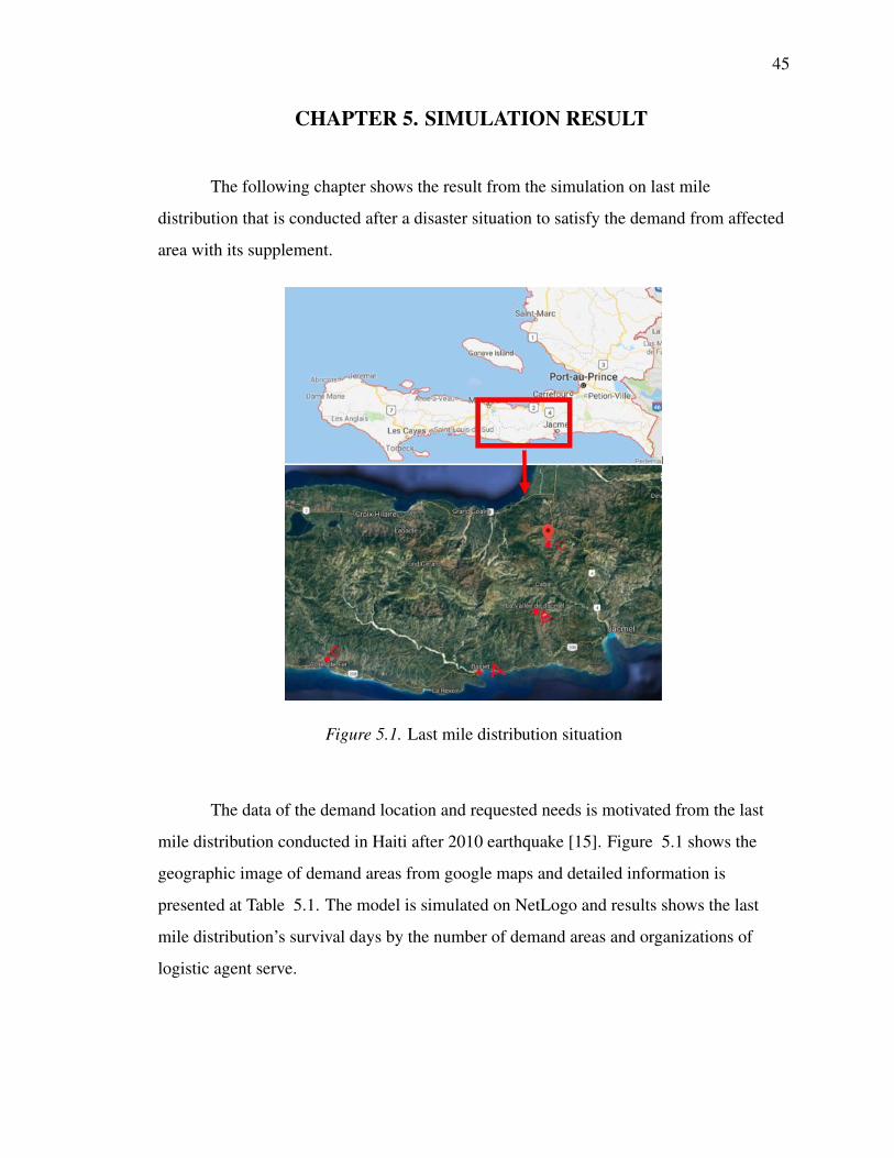
45
CHAPTER 5. SIMULATION RESULT
The following chapter shows the result from the simulation on last mile
distribution that is conducted after a disaster situation to satisfy the demand from affected
area with its supplement.
Figure 5.1. Last mile distribution situation
The data of the demand location and requested needs is motivated from the last
mile distribution conducted in Haiti after 2010 earthquake [15]. Figure 5.1 shows the
geographic image of demand areas from google maps and detailed information is
presented at Table 5.1. The model is simulated on NetLogo and results shows the last
mile distribution’s survival days by the number of demand areas and organizations of
logistic agent serve.

46
Table 5.1. Last mile distribution situation
Demand Areas
Baniet(Da) La Vallee(Db) Trouin(Dc) Cotes-de-Fer(Dd)
Distance(km) 45 16 41 79
Needs(kg) 24243 13701 10183 6737
5.1 last mile distribution
The result presented in this section shows the survival years of last mile
distribution where the allocation agent assigns the logistic agent for the humanitarian
logistic. The allocation agent evaluates an adequate demand area where logistic agents are
deemed to fit for delivering the relief items. An assignment is given to logistic agents who
have high priority, and it is decided based on the number of trips that logistic agents have
done for last mile distribution previously. As the logistic agents have exerted themselves
with the more logistic task, logistic agents are given lower priority for assignment. Once a
demand area is assigned to logistic agents, the area will not be changed until the end of the
day. From the result presented below, the last mile distribution’s survival years can be
found and its relation with the number of logistic agents in operation.
5.1.1 Allocating with Truck A(Ta)
As can be seen from Figure 5.2(a), assigning one Truck A can satisfy the needs of
the demand area A, Baniet for about 10 days. Instead, putting two A Trucks into operation
survives the last mile distribution for at least 6 years from the simulation result. From the
result, the survival year shows the trend of increasing as the number of the logistic agent
assigned into operation increased to the point of total 4 logistic agents. When the number
of A-type trucks placed in this last mile distribution is four, the supplement can survive for

47
(a) One Demand Area - Baniet
(b) Two Demand Areas - Baniet, La Vallee
(c) Three Demand Areas - Baniet, La Vallee, Trouin
(d) Four Demand Areas - Baniet, La Vallee, Trouin,Cotes-de-Fer
Figure 5.2. Truck A(Ta) Organization’s last mile distribution
48
8 years. However, the survival time will decrease when the A-type truck is over four.
When five trucks are placed in the last mile distribution and follow the assignment from
allocation agent, the logistics will survive only for 5 years which is shorter than four
trucks’ last mile distribution survival year. From the result, the A-type truck placement on
last mile distribution for one demand area is advised to be between two and four trucks.
When the last mile distribution includes the other area which is La-Valle, the relief
organization should serve two demand areas. Figure 5.2(b) shows that the number of
truck A to be placed at the local distribution center is different. Two trucks are not enough
to satisfy the need from two demand area simultaneously, for even a day. However, three
A trucks can survive the logistics for more than 6 years. Even surviving for seven years is
possible with the five A trucks allocated at Local Distribution Center.
In the third case, the relief aids should be delivered to three areas which are Baniet,
La Vallee, and Trouin. As can be seen from Figure 5.2(c), four A trucks are needed for
successful logistics for six years. The survival year can be increased when more than four
logistic agents are placed to the local distribution center, and 7 A-type trucks show the
most extended survival year with 8 years. If more logistic agents than 7 A trucks are
placed, However, the survival year of last mile distribution is shown to be decreased.
The last Figure 5.2(d) shows how many years the logistic can survive when one
local distribution center should conduct last mile distribution for four demand areas which
are Baniet, La Vallee, Trouin, and Cotes-de-Fer. Needs from four areas to be fulfilled for a
day, five A truck should be placed for the operation, minimally. If a fewer number than
five A trucks are put into the operation, they can not deliver a sufficient amount of relief
items that are needed for areas even they continuously work all the time. When more than
five A type trucks are allocated to the operation, the last mile can survive for 6 years. With
7 trucks, the last mile distribution shows the best performance from the perspective of
survival years as they can continue the operation for nearly 8 years. However, the survival
year can be decreased when more than 8 A trucks are placed in the last mile distribution.

49
5.1.2 Allocating with Truck B(Tb)
Compared to Truck A, Truck B can survive the logistics to the one demand, Baniet
with only one truck for 6 years. As the loading capacity of the B truck is more prominent
than the Truck A, a Truck B can supply the amount of relief aid that two A trucks can do.
As presented in Figure 5.3(a), distribution can survive for 8 years With the organization
formed with two B trucks. However, putting more than 3 B trucks show shorter survival
years than survival years with one or two trucks. From the perspective of finance and
survivability, therefore, putting one or two B trucks is beneficial for relief aids
organization.
When it comes to serving two demand areas, Baniet, and La Vallee, the survival
years are shown in Figure 5.3(b). As the number of demand areas served increases, one
truck B is not enough for satisfying the need for both areas. Therefore, at least two B
trucks are needed to deliver the amount of relief aids that needed to demand areas.
Allocating three B trucks show the most extended survival years in this case by surviving
more than 8 years. However, putting more than 3 trucks decrease the survival years to the
point where they can satisfy the demand by 4 years.
The third case presents the situation where LDC should serve the last mile
distribution to three areas and the survival years can be found from Figure 5.3(c). For
distributing relief items to three areas, the number of B trucks that should be put into
operation is three. The distribution can survive for more than 7 years when the three
trucks continuously deliver items to the designated areas as their total loading capacity
become over than 48,127kg which is total need from three demand areas. With four B
trucks, the affected people can get a steady supply from LDC for 8 years. However, more
than five B trucks’ last mile distribution show fewer survival years even though it can
serve more than three years.

50
(a) One Demand Area - Baniet
(b) Two Demand Areas - Baniet, La Vallee
(c) Three Demand Areas - Baniet, La Vallee, Trouin
(d) Four Demand Areas - Baniet, La Vallee, Trouin,Cotes-de-Fer
Figure 5.3. Truck B(Tb) Organization’s last mile distribution

51
When four areas need the relief aids and only B trucks can be placed to the areas,
the LDC requires four B trucks as the number of areas where they can be distributed to is
four. According to the result presented from Figure 5.3(d), assigning 5 B trucks into
operation will survive the distribution for 8 years. However, placing a bigger number of B
trucks than 5 rather decrease the survival years.
5.1.3 Allocating with Helicopter A(Ha)
Compared to trucks, helicopters’ loading capacity is much smaller. Therefore, the
helicopters require many trips from LDC to demand areas to deliver the amount requested
from these areas. However, helicopters are much faster than trucks which compensate for
the weakness. Specifically, Helicopter A defined in this study can carry 2 tons of items at
a time and fly with a speed of 217km/h.
The first Figure 5.4(a) shows the case where the allocation agent needs Helicopter
A for last mile distribution to one area, Baniet which requires 24,243 kg of items per day.
As the size of needs are enormous for one A helicopter to carry, A helicopters require
many trips. However, the round of trips they can do is limited which results in
non-survival even with two A helicopters on the operation. As the number of Helicopters
comes to three, the logistics can survive for 8 years. Also, survival years presented from
the result shows an increasing trend from three to nine A helicopters placement. Having
more than 10 A helicopters for the distribution increase the possibility where logistic
agents can encounter the immediate danger of inoperable status from insufficient uses.
The second case of serving two demand areas, the allocation agents require at least
five A type helicopters to deliver relief items matched to request. As the second area, La
Vallee requires 13,701 kg of items which is significant for A helicopters to finish
delivering in a day alone. Figure 5.4(b) shows that organizations consisting of more than
five A helicopters survive logistics for at least 8 survival year. Especially, logistics can
survive for 10 years when 11 A helicopters are placed to the organization. However,
putting more than 12 helicopters instead decrease the burden on other helicopters but put
them into the danger of sudden incapacity from improper uses.
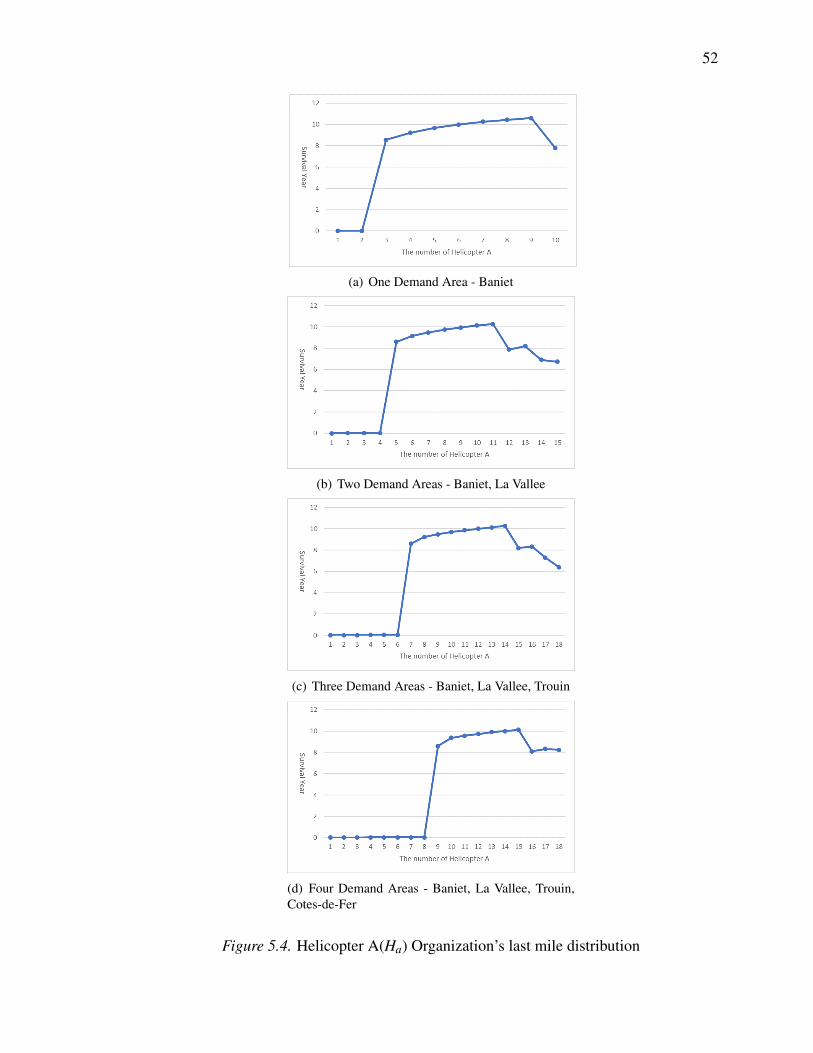
52
(a) One Demand Area - Baniet
(b) Two Demand Areas - Baniet, La Vallee
(c) Three Demand Areas - Baniet, La Vallee, Trouin
(d) Four Demand Areas - Baniet, La Vallee, Trouin,Cotes-de-Fer
Figure 5.4. Helicopter A(Ha) Organization’s last mile distribution
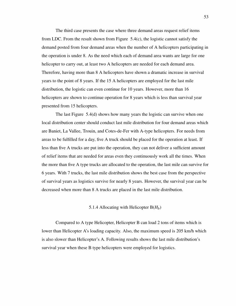
53
The third case presents the case where three demand areas request relief items
from LDC. From the result shown from Figure 5.4(c), the logistic cannot satisfy the
demand posted from four demand areas when the number of A helicopters participating in
the operation is under 8. As the need which each of demand area wants are large for one
helicopter to carry out, at least two A helicopters are needed for each demand area.
Therefore, having more than 8 A helicopters have shown a dramatic increase in survival
years to the point of 8 years. If the 15 A helicopters are employed for the last mile
distribution, the logistic can even continue for 10 years. However, more than 16
helicopters are shown to continue operation for 8 years which is less than survival year
presented from 15 helicopters.
The last Figure 5.4(d) shows how many years the logistic can survive when one
local distribution center should conduct last mile distribution for four demand areas which
are Baniet, La Vallee, Trouin, and Cotes-de-Fer with A-type helicopters. For needs from
areas to be fulfilled for a day, five A truck should be placed for the operation at least. If
less than five A trucks are put into the operation, they can not deliver a sufficient amount
of relief items that are needed for areas even they continuously work all the times. When
the more than five A type trucks are allocated to the operation, the last mile can survive for
6 years. With 7 trucks, the last mile distribution shows the best case from the perspective
of survival years as logistics survive for nearly 8 years. However, the survival year can be
decreased when more than 8 A trucks are placed in the last mile distribution.
5.1.4 Allocating with Helicopter B(Hb)
Compared to A type Helicopter, Helicopter B can load 2 tons of items which is
lower than Helicopter A’s loading capacity. Also, the maximum speed is 205 km/h which
is also slower than Helicopter’s A. Following results shows the last mile distribution’s
survival year when these B type helicopters were employed for logistics.

54
(a) One Demand Area - Baniet
(b) Two Demand Areas - Baniet, La Vallee
(c) Three Demand Areas - Baniet, La Vallee, Trouin
(d) Four Demand Areas - Baniet, La Vallee, Trouin,Cotes-de-Fer
Figure 5.5. Helicopter B(Hb) Organization’s last mile distribution
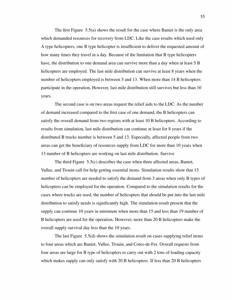
55
The first Figure 5.5(a) shows the result for the case where Baniet is the only area
which demanded resources for recovery from LDC. Like the case results which used only
A type helicopters, one B type helicopter is insufficient to deliver the requested amount of
how many times they travel in a day. Because of the limitation that B type helicopters
have, the distribution to one demand area can survive more than a day when at least 5 B
helicopters are employed. The last mile distribution can survive at least 8 years when the
number of helicopters employed is between 5 and 13. When more than 14 B helicopters
participate in the operation, However, last mile distribution still survives but less than 10
years.
The second case is on two areas request the relief aids to the LDC. As the number
of demand increased compared to the first case of one demand, the B helicopters can
satisfy the overall demand from two regions with at least 10 B helicopters. According to
results from simulation, last mile distribution can continue at least for 8 years if the
distributed B trucks number is between 5 and 13. Especially, affected people from two
areas can get the beneficiary of resources supply from LDC for more than 10 years when
13 number of B helicopters are working on last mile distribution. Survive
The third Figure 5.5(c) describes the case when three affected areas, Baniet,
Vallee, and Trouin call for help getting essential items. Simulation results show that 15
number of helicopters are needed to satisfy the demand from 3 areas when only B types of
helicopters can be employed for the operation. Compared to the simulation results for the
cases where trucks are used, the number of helicopters that should be put into the last mile
distribution to satisfy needs is significantly high. The simulation result present that the
supply can continue 10 years in minimum when more than 15 and less than 19 number of
B helicopters are used for the operation. However, more than 20 B helicopters make the
overall supply survival day less than the 10 years.
The last Figure 5.5(d) shows the simulation result on cases supplying relief items
to four areas which are Baniet, Vallee, Trouin, and Cotes-de-Fer. Overall requests from
four areas are large for B type of helicopters to carry out with 2 tons of loading capacity
which makes supply can only satisfy with 20 B helicopters. If less than 20 B helicopters

56
are placed to LDC, the logistic cannot meet the need from areas unless they are going to
the multiple demands a day. Placing 20, 21 and 22 number of B helicopters to the
operation survived supply for 8 years, but placing more number of B helicopters is shown
to have fewer survival years which is not ideal.
As can be seen from above simulation results, the number of logistic agents have a
significant effect on last mile distribution’s survival years since how many years the last
mile distribution can continue heavily depends on the type and number of logistic agents
placed on logistic. Therefore, the result can be the source for deciding how many logistic
agents should be placed for the cases. As presented from the result, the large number of
logistic agents does not guarantee long survival years. It is because the excessive number
of logistics agent placed on the distribution rather put agents into the danger of
unexpected incapacity such as battery drain for long term idle status. Therefore, placing
the appropriate number of logistic agents that can survive through the scheduled operation
is important.
5.2 Multiple kinds of logistic agents
This section presents the cases where multiple kinds of logistic agents are needed
for last mile distribution. Each logistic agents type has different advantages and
disadvantages on its speeding and loading capacity. Therefore, it is also important to see
the logistics’ survivability when there are multiple kinds of logistic agents do the task for
the last mile distribution. Following results show the last mile distribution’s survival days
when a number of different types of logistic agents which shown the longest survival days
individually work together for last mile distribution to four different demand areas.

57
5.2.1 Allocating Truck A(Ta) and Truck B( Tb)
According to the survivability result when A-type trucks are individually
simulated, the last mile distribution reveals to have the longest survival days when 7
number of A-type trucks are allocated to the LDC. On the other hand, allocating 5 trucks
shows the long survival duration when it comes to B type trucks. Therefore, allocating
both of 7 A type trucks and 5 B type trucks to last mile distribution are simulated to see
the survival days and results show that they can survive the last mile distribution only for
3.8 years which is significantly short survival years compared to the survivability they
made individually. It is because the total number of logistic agents are excessive in this
last mile distribution. Therefore, additional cases under the number that individually
shown the best survivability were simulated. Following Table 5.2 presents the extreme
cases of logistic survivability with a combination of Truck A and Truck B. As can be seen,
the survivability can be obtained to the extent of more than 8 years when two Truck A and
5 Truck B are allocated. The cases showing the high survivability have a trend of having 6
logistic agents in total and more B type Trucks, rather than A trucks. Contrary to cases
having high survivability, the cases show weak survivability when the total logistic agents
employed to the operation comes to under four, especially shows non-survival when
logistic agents are under three.
Table 5.2. Extreme Logistic Survivability cases with Truck A(Ta) and Truck B(Tb)
A Truck(Ta) B Truck(Tb) Survival Year
2 5 8.347436322
1 5 8.342675272
1 4 8.061967775
.. .. ..
1 2 0.002392558
2 1 0.002357258
1 1 0.00185934

58
5.2.2 Allocating Truck A(Ta) and Helicopter A( Ha)
In this case, allocating A trucks and A helicopters on distribution was simulated. A
type of helicopters showed the best survivability when 15 A helicopters were allocated.
Therefore, 15 A helicopters are employed together with 7 A trucks to last mile distribution
and results show that last mile distribution continues for 4.1 years. This is also short
survival years compared to individual survivability shown at previous simulation. As
employing total of 22 numbers of logistic agents is deemed to be ineffective for logistics
survivability, further logistic agents combinations under 22 total logistic agents are
simulated and the extreme cases are shown in Table 5.3. The table shows that the
survivability can be gained to the extent of more than 10 years when a total of 15 logistic
agents are employed, and helicopter A takes the most in the organization. Even though
one Truck A would be not sufficient to satisfy the needs from four demand areas, the
survivability can be achieved in the extreme when it is allocated with the proper number
of helicopter A.
Table 5.3. Extreme Logistic Survivability cases with Truck A(Ta) and Helicopter A(Ha)
A Truck(Ta) A Helicopter(Ha) Survival Year
1 14 10.16220992
2 13 10.14809998
.. .. ..
2 6 0.006780251
1 7 0.005391362
1 6 0.005391362
.. .. ..
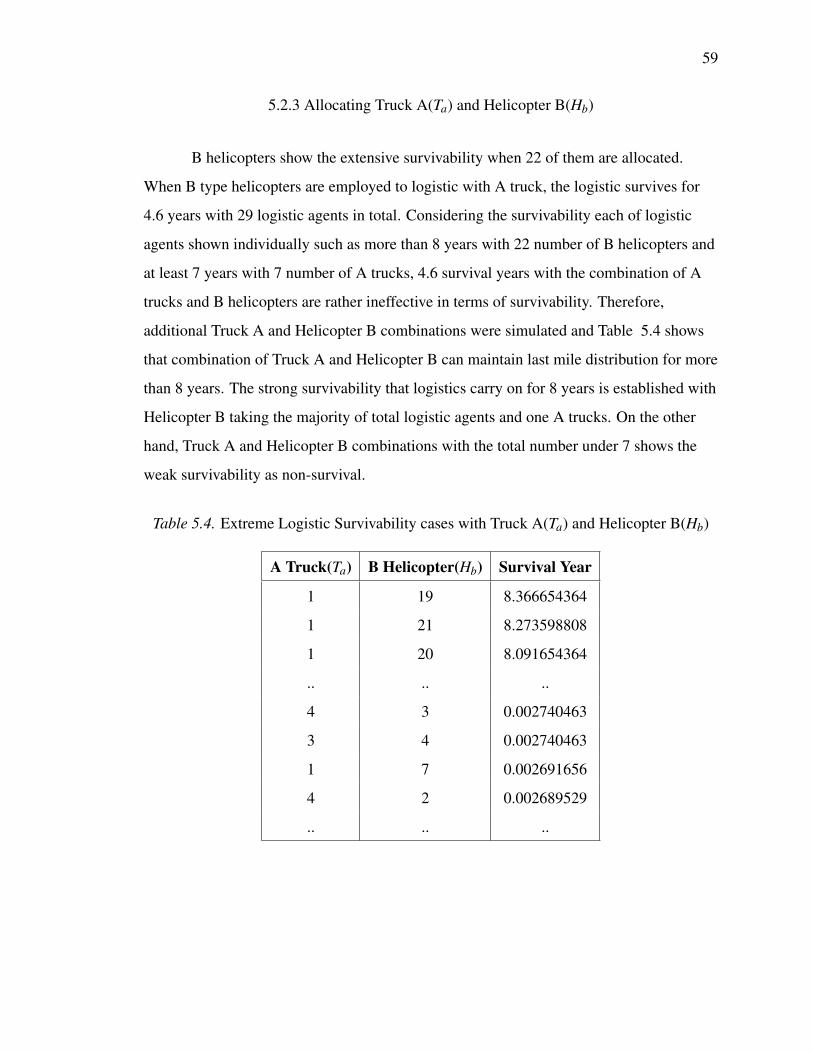
59
5.2.3 Allocating Truck A(Ta) and Helicopter B(Hb)
B helicopters show the extensive survivability when 22 of them are allocated.
When B type helicopters are employed to logistic with A truck, the logistic survives for
4.6 years with 29 logistic agents in total. Considering the survivability each of logistic
agents shown individually such as more than 8 years with 22 number of B helicopters and
at least 7 years with 7 number of A trucks, 4.6 survival years with the combination of A
trucks and B helicopters are rather ineffective in terms of survivability. Therefore,
additional Truck A and Helicopter B combinations were simulated and Table 5.4 shows
that combination of Truck A and Helicopter B can maintain last mile distribution for more
than 8 years. The strong survivability that logistics carry on for 8 years is established with
Helicopter B taking the majority of total logistic agents and one A trucks. On the other
hand, Truck A and Helicopter B combinations with the total number under 7 shows the
weak survivability as non-survival.
Table 5.4. Extreme Logistic Survivability cases with Truck A(Ta) and Helicopter B(Hb)
A Truck(Ta) B Helicopter(Hb) Survival Year
1 19 8.366654364
1 21 8.273598808
1 20 8.091654364
.. .. ..
4 3 0.002740463
3 4 0.002740463
1 7 0.002691656
4 2 0.002689529
.. .. ..

60
5.2.4 Allocating Truck B(Tb) and Helicopter A(Ha)
When 5 B type trucks and 15 A type helicopters cooperate for the last mile
distribution, the survival days is shown to be 4.2 years. This result showed a similar trend
when the logistic was simulated for the case where both of A trucks and A helicopters
were employed together at last mile.
74 more cases are simulated to find the logistics survivability with the combination
of Truck B and Helicopter A. From the part of results presented in Table 5.5, logistics
could survive more than 10 years when more than 8 Helicopter A are placed to the last
mile distribution with 1 Truck B. When the number of Truck B employed for the operation
is one or two, and the total number of logistic agents in organizations is under 6, the last
mile distribution could not satisfy the needs from four different areas.
Table 5.5. Extreme Logistic Survivability Cases with Truck B(Tb) and Helicopter A(Ha)
B Truck(Tb) A Helicopter(Ha) Survival Year
1 14 10.26109881
1 13 10.13609881
.. .. ..
2 3 0.002717882
2 2 0.002717882
1 4 0.002479869
2 4 0.002461693
.. .. ..

61
5.2.5 Allocating Truck B(Tb) and Helicopter B(Hb)
When solely B type trucks were assigned to the task of delivering relief aids to
four demand areas, 5 trucks could continue logistics for more than 8 years. Also, B type
helicopters survived distribution for almost 8 years with 22 helicopters. However, when
the distribution is conducted with a total of 27 logistic agents, last mile distribution only
survived for 4.5 years. From the extensive simulations, the last mile distribution with the
union of Truck B and Helicopter B is revealed to be survivable for about 8 years. As can
be seen from Table 5.6 presenting extreme cases of logistic survivability, the logistics
have strong survivability when one Truck B is employed with 15 to 21 Helicopter B. Also,
the cases where 5 B Trucks are employed could keep its operation continuously more than
8 years when those cooperates with under 15 B Helicopters.
Table 5.6. Extreme Logistic Survivability Cases with Truck B(Tb) and Helicopter B(Hb)
B Truck(Tb) B Helicopter(Hb) Survival Year
1 21 8.63332103
1 20 8.544432141
1 19 8.513876586
.. .. ..
4 3 0.001107379
4 2 0.001107379
4 1 0.001107379
3 4 0.0011073797
.. .. ..

62
5.2.6 Allocating Helicopter A(Ha) and Helicopter B(Hb)
This case presents when helicopters A and B participate in a logistic task together,
and Table 5.7 shows its extreme cases. Even though the operation is immense including
overall 37 logistic agents, last mile distribution only survives for about 4.7 years which
shows not much increase in survivability compared to the case where 5 A trucks and 15 A
helicopters are cooperating. However, the additional simulations where both kinds of
helicopters are delivering together were conducted, it is founded that survivability can be
achieved for more than 10 years. Especially, delivering with helicopters are shown to have
strong survivability in many cases compared to other situations where the combination of
truck and helicopter, or only trucks are operating. 7.2% of cases are shown to have more
than 9 years survivability which is higher than other cases’ proportion.
Table 5.7. Extreme Logistic Survivability Cases with Helicopter A(Ha) and HelicopterB(Hb)
A Helicopter(Ha) B Helicopter(Hb) Survival Year
7 12 10.12736043
8 11 10.11347154
5 14 10.08486151
.. .. ..
8 4 0.002765475
7 5 0.002765475
7 4 0.002765475
6 6 0.002765475
.. .. ..
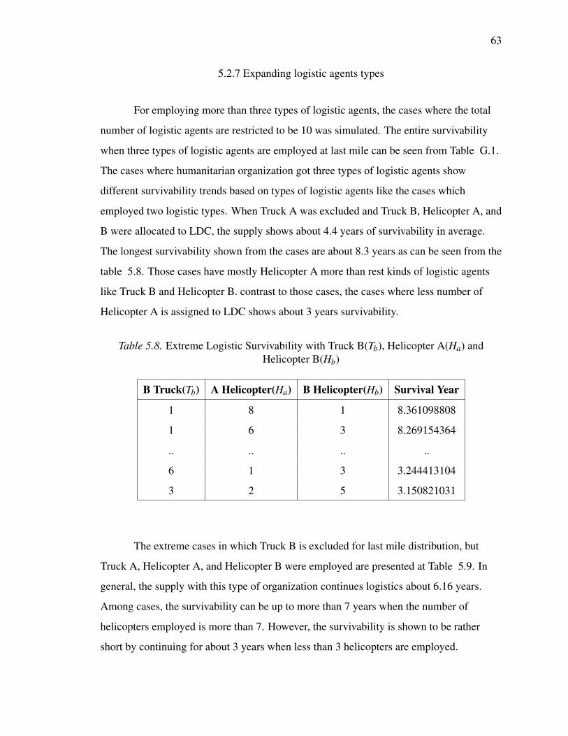
63
5.2.7 Expanding logistic agents types
For employing more than three types of logistic agents, the cases where the total
number of logistic agents are restricted to be 10 was simulated. The entire survivability
when three types of logistic agents are employed at last mile can be seen from Table G.1.
The cases where humanitarian organization got three types of logistic agents show
different survivability trends based on types of logistic agents like the cases which
employed two logistic types. When Truck A was excluded and Truck B, Helicopter A, and
B were allocated to LDC, the supply shows about 4.4 years of survivability in average.
The longest survivability shown from the cases are about 8.3 years as can be seen from the
table 5.8. Those cases have mostly Helicopter A more than rest kinds of logistic agents
like Truck B and Helicopter B. contrast to those cases, the cases where less number of
Helicopter A is assigned to LDC shows about 3 years survivability.
Table 5.8. Extreme Logistic Survivability with Truck B(Tb), Helicopter A(Ha) andHelicopter B(Hb)
B Truck(Tb) A Helicopter(Ha) B Helicopter(Hb) Survival Year
1 8 1 8.361098808
1 6 3 8.269154364
.. .. .. ..
6 1 3 3.244413104
3 2 5 3.150821031
The extreme cases in which Truck B is excluded for last mile distribution, but
Truck A, Helicopter A, and Helicopter B were employed are presented at Table 5.9. In
general, the supply with this type of organization continues logistics about 6.16 years.
Among cases, the survivability can be up to more than 7 years when the number of
helicopters employed is more than 7. However, the survivability is shown to be rather
short by continuing for about 3 years when less than 3 helicopters are employed.

64
Table 5.9. Extreme Logistic Survivability with Truck A(Ta), Helicopter A(Ha) andHelicopter B(Hb)
A Truck(Ta) A Helicopter(Ha) B Helicopter(Hb) Survival Year
3 6 1 7.591654364
3 5 2 7.591654364
.. .. .. ..
6 2 2 3.691151099
6 1 3 3.388802767
The third case for employing three kinds of logistic agents is assigning two kinds
of trucks and Helicopter B. These cases are presented to survive logistics for 4.4 years on
average. Contrast to other cases which employed Helicopter A, cases which exclude
Helicopter A show 6 survival years at most as can be found from extreme cases presented
at Table 5.10. Even, the case indicates that logistics can survive only 2 years which is
never seen from other cases employing Helicopter A.
Table 5.10. Extreme Logistic Survivability with Truck A(Ta), Truck B(Tb) and HelicopterB(Hb)
A Truck(Ta) B Truck(Tb) B Helicopter(Hb) Survival Year
2 1 7 6.018851575
3 1 6 5.975770886
.. .. .. ..
2 3 5 3.086171493
1 5 4 2.969576073
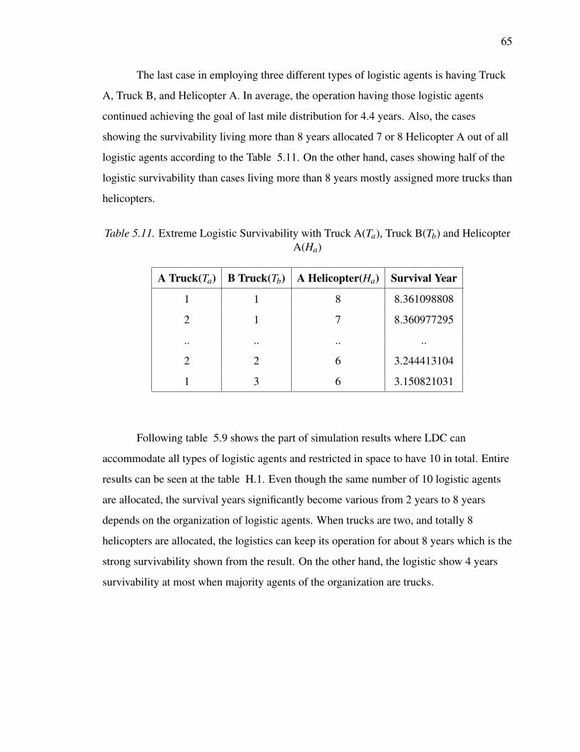
65
The last case in employing three different types of logistic agents is having Truck
A, Truck B, and Helicopter A. In average, the operation having those logistic agents
continued achieving the goal of last mile distribution for 4.4 years. Also, the cases
showing the survivability living more than 8 years allocated 7 or 8 Helicopter A out of all
logistic agents according to the Table 5.11. On the other hand, cases showing half of the
logistic survivability than cases living more than 8 years mostly assigned more trucks than
helicopters.
Table 5.11. Extreme Logistic Survivability with Truck A(Ta), Truck B(Tb) and HelicopterA(Ha)
A Truck(Ta) B Truck(Tb) A Helicopter(Ha) Survival Year
1 1 8 8.361098808
2 1 7 8.360977295
.. .. .. ..
2 2 6 3.244413104
1 3 6 3.150821031
Following table 5.9 shows the part of simulation results where LDC can
accommodate all types of logistic agents and restricted in space to have 10 in total. Entire
results can be seen at the table H.1. Even though the same number of 10 logistic agents
are allocated, the survival years significantly become various from 2 years to 8 years
depends on the organization of logistic agents. When trucks are two, and totally 8
helicopters are allocated, the logistics can keep its operation for about 8 years which is the
strong survivability shown from the result. On the other hand, the logistic show 4 years
survivability at most when majority agents of the organization are trucks.

66
Table 5.12. Extreme Cases of last mile distribution to Demand with all logistic agents
A Truck(Ta) B Truck(Tb) A Helicopter(Ha) B Helicopter(Hb) Survival Year
1 1 7 1 8.361098808
1 1 6 2 8.133866764
1 1 5 3 8.8.35042174
1 1 4 4 8.301274637
.. .. .. .. ..
1 5 1 3 4.385886029
1 7 1 1 4.373147885
4 3 2 1 4.348341657
4 2 3 1 4.305407614

67
CHAPTER 6. CONCLUSION AND FUTURE WORK
6.1 Conclusion
Through simulations, the emergent situations where logistic agents have
unexpected incapability to deliver relief aid to destined demand areas are shown. In a real
situation where the continuous supply is essential as the case of Typhoon Haiyan, the
sudden stop on distribution puts significant strain on the recovery process. This study
inquires the last mile distribution’s survivability after the disaster with organization of
logistic agents. By simulating multiple logistic agents which can be employed in last-mile
distribution, this study shows that the logistic survivability depends on the number of
logistic agents employed to the distribution. Assigning as many logistic agents as possible
is revealed to be not ideal for logistic survivability as could be seen from the simulation
result that increased the agent number employed in the same environment. Consistently,
logistic agents experience the downtrend in the survival at a certain size of the
organization. For the last mile distribution to four different areas, following logistics’
survivability is observed when different kinds of logistic agents were used solely.
• Employing Truck A showed the uptrend until the total number of Truck A is 7, but
assigning more than 8 A trucks showed rather decreased survival compared to a
smaller organization.
• Employing Truck B survives the logistics at most 8 years when the size of the
organization is up to 5, but bigger organizations formed with more than 6 B trucks
show a decreasing trend in survivability.
• Employing Helicopter A shows the uptrend when the organization formed with
from 9 to 15 A helicopters, but the survival reduces when bigger organizations
formed with more than 16 A helicopters are employed.

68
• Employing Helicopter B survives logistics when organizations are established with
more than 20 B Helicopters. Organizations with more than 23 Helicopter B display
shorter survivability than the smaller organization.
If an excessive number of logistic agents are employed at the last mile distribution,
the logistics chance to survive is reduced because the possibility of unexpected agent
failure is increased. Because logistic agents are idle and not utilized, negative impacts are
produced on lifespan, as much as, the ones which are frequently used for the last mile
distribution.
Also, logistics’ survivability depends not only on the size of the organization but
also which type of logistic agents formed logistic organizations.
• When A Truck and B Truck are assigned to the distribution, the logistics survive for
8 years with logistic agent organization formed with 2 A trucks and 5 B trucks.
• When A Truck and A Helicopter are employed, the organization consisted of 1 A
truck and 14 A helicopter survives logistic for 10 years.
• When A Truck and B Helicopter are assigned to the distribution, the organization
formed with 1 A truck and 19 B Helicopters continues last mile distribution for 8
years.
• When B Truck and A Helicopter are assigned, the distribution survivability shows a
similar trend with the one employed the organization of A truck and A Helicopter.
The organization consisted of 1 B truck and 14 A trucks survives logistics for 10
years.
• When B Truck and B Helicopter are employed together, the logistics organized with
1 B truck and 21 Helicopters survive for 8 years.
• When A Helicopter and B Helicopter are employed, the organization formed with 7
A Helicopters and 12 B Helicopters distribute resources for 10 years at most.

69
Table 6.1. Summary of Logistics Survivability Bast Cases - Two Logistic Agent TypeOrganization
A Truck(Ta) B Truck(Tb) A Helicopter(Ha) B Helicopter(Hb) Survival Year
2 5 - - 8
1 - 14 - 10
1 - - 19 8
- 1 14 - 10
- 1 - 21 8
- - 7 12 10
Following Table 6.1 shows the summary of best logistics survivability cases when
the organization formed with two kinds of logistic agents. Except for the organization that
two kinds of trucks are involved in, the cases that the helicopter takes the significant part
in organization showed the best survivability.
When LDC restricted the logistics organization’s size to be 10 and allow more than
three types of logistic agents to be organized for last mile distribution, following
survivability can be observed.
• When three types of the logistic agent which are B Truck, A Helicopter, and B
Helicopter are to be assigned, the organization formed with 1 B Truck, 8 A
Helicopters, and 1 B Helicopter survives the distribution for 8 years.
• When three types of the logistic agent which are A Truck, A Helicopter, and B
Helicopter are to be assigned, the organization formed with 3 A Trucks, 6 A
Helicopters, and 1 B Helicopter survives the distribution for 7 years.
• When three types of the logistic agent which are A Truck, B Truck, and A
Helicopter are to be assigned, the organization formed with 2 A Trucks, 1 B Truck,
and 7 A Helicopter survives the distribution for 6 years.

70
• When three types of the logistic agent which are A Truck, B Truck, and A
Helicopter are to be assigned, the organization formed with 1 A Trucks, 1 B Trucks,
and 8 B Helicopter survives the distribution for 8 years.
• When all logistic types of agents can be assigned, the organization formed with 1 A
Truck, 1 B Truck, 7 A Helicopter, and 1 B Helicopter survives the distribution for 8
years.
Table 6.2. Summary of Logistics Survivability Bast Cases - Organization with 10 logisticagents
A Truck(Ta) B Truck(Tb) A Helicopter(Ha) B Helicopter(Hb) Survival Year
- 1 8 1 8
3 - 6 1 10
2 1 - 7 6
1 1 8 - 8
1 1 7 1 8
Following Table 6.2 shows the best survivability cases when LDC restricted the
size of logistic organizations to be 10 and more than three kinds of logistic agents are
assigned. As can be seen from the Table 6.2, each case showing the like the best
survivability have organizations taken majority of occupants with helicopters like the
trend shown from cases having organization formed with two kinds of logistic agents.
Depends on type of logistic agents consisting organization, the survival showed
different trend. Even though the total number of logistic agents assigned to local
distribution center is same, how long last mile distribution survives vary by which type of
logistic agents are the major of organization. Consistently, helicopters are shown to be
beneficiary for strong survivability as organizations that helicopters occupy significant
parts display long survivability.

71
For humanitarian logistic, it is significantly important to make logistics survivable
for the duration of time. Unexpected stop on continuous supply prevents affected areas to
recover and prolongs the suffering. However, those risks increase as logistic agents which
have critical role in delivering items suffer from harsh operation. Therefore, this study
researched logistic survivability with the consideration on logistic agents’ susceptibility to
humanitarian operations. Eventually, this research found different trends in logistic
survivability depends on sizes and arrangements of logistic agent organizations and
optimal organization having strong survivability by situations.
6.2 Future Work
This study assumes that logistic agents are a set of one transportation vehicle and
one driver or pilot. Also, drivers will be always available when the vehicle should be
operated is assumed. However, there are chances that drivers are not available for the
operation which would be critical considering professionalism required for vehicles to be
operated. Therefore, logistics’ survivability when human logistic agents are susceptible to
the environment can be further studied. For last mile distribution especially for the
humanitarian logistic, the role of human logistic agents are important as vehicles because
various things can affect them in ways. Therefore, the professional human logistic agents
and human agents organizations to survive last mile distribution can be further researched.
Also, this study assumes that the demand from each areas are consistent, but it can
become vary by the stage of recovery. As the later stage of recovery involves in
infrastructure, the requested items and its size would grow. Accords to stages of recovery,
the logistic transport agent and human agent organization that can survive the change in
stage can be more studied.
For humanitarian logistic, it is also important not to make excessive waste on
budget and survive at the same time. Last mile distribution requires a notable budget for
overall management by taking the second largest proportion of the total expense that
humanitarian aid organizations spend for overall aid operation [15]. As the expense is
secured from the donation, the properly managing the expense in logistic will enhance the
72
credibility and effectiveness in providing aids with allocating much expense on procuring
relevant resources for recovery. From the result, the excessive allocation of logistic agents
is revealed to not increase the survivability at a certain point and different survivability
depends on the composition of organizations. Allocating more logistic agents than needed
can not only decrease the survivability of logistic and chance that the budget could be used
for a more needed part in the humanitarian operation. Therefore, logistic agent
organizations that could give credibility by surviving logistics and reducing excessive cost
can be further studied.
73
REFERENCES
[1] I. M. Shaluf, “Disaster types,” Disaster Prevention and Management: An
International Journal, vol. 16, no. 5, pp. 704–717, 2007.
[2] “Terminology - UNISDR,” 2017. [Online]. Available:
https://www.unisdr.org/we/inform/terminology#letter-d
[3] R. Wallemacq, Pascaline; House, “Economic losses, poverty & disasters: 1998-2017,”
11 2018. [Online]. Available:
https://www.unisdr.org/we/inform/publications/61119
[4] United Nations International Strategy for Disaster Reduction(UNISDR), “Impacts of
Disasters since the 1992 Rio de Janeiro Earth Summit,” 2012. [Online].
Available: https://www.unisdr.org/files/27162 infographic.pdf
[5] B. Balcik, B. M. Beamon, and K. Smilowitz, “Last mile distribution in humanitarian
relief,” Journal of Intelligent Transportation Systems: Technology, Planning,
and Operations, vol. 12, no. 2, pp. 51–63, 2008.
[6] J. Perlah, “After Typhoon Haiyan, Philippines Economy Grows At Slowest Pace In
Over A Year,” 2013. [Online]. Available: https://www.ibtimes.com/
after-typhoon-haiyan-philippines-economy-grows-slowest-pace-over-year-1489028
[7] D. Mersereau, “Why so many people died from Haiyan and past southeast Asia
typhoons - The Washington Post,” 2013. [Online]. Available:
https://www.washingtonpost.com/news/capital-weather-gang/wp/2013/11/11/
inside-the-staggering-death-toll-from-haiyan-and-other-southeast-asia-typhoons/
?noredirect=on&utm term=.22380dba29be

74
[8] T. Branigan and K. Hodal, “Typhoon Haiyan: frustration at slow pace of relief effort
— World news — The Guardian,” 2013. [Online]. Available:
https://www.theguardian.com/world/2013/nov/14/
typhoon-haiyan-relief-effort-stalls-philippines
[9] M. Ahmadi, A. Seifi, and B. Tootooni, “A humanitarian logistics model for disaster
relief operation considering network failure and standard relief time: A case
study on San Francisco district,” Transportation Research Part E: Logistics
and Transportation Review, vol. 75, pp. 145–163, 2015. [Online]. Available:
http://dx.doi.org/10.1016/j.tre.2015.01.008
[10] M. F. Maghfiroh and S. Hanaoka, “Last mile distribution in humanitarian logistics
under stochastic and dynamic consideration,” in 2017 IEEE International
Conference on Industrial Engineering and Engineering Management (IEEM).
Singapore: IEEE, 2018, pp. 1411–1415.
[11] F. R. Jack Healy and R. Nixon, “Aid Is Getting to Puerto Rico. Distributing It
Remains a Challenge. - The New York Times.” [Online]. Available:
https://www.nytimes.com/2017/10/03/us/puerto-rico-aid-fema-maria.html
[12] S. J. Russell, P. Norvig, J. F. Canny, J. M. Malik, D. D. Edwards, and S. J. S.
Jonathan, Artificial Intelligence: a modern approach, 1995, vol. 13, no. 2.
[Online]. Available: http://www.ncbi.nlm.nih.gov/pubmed/21104209
[13] W. Wisetjindawat, H. Ito, M. Fujita, and H. Eizo, “Planning Disaster Relief
Operations,” Procedia - Social and Behavioral Sciences, vol. 125, pp.
412–421, 2014. [Online]. Available:
http://linkinghub.elsevier.com/retrieve/pii/S1877042814015225

75
[14] J. M. Day, S. A. Melnyk, P. D. Larson, E. W. Davis, and D. C. Whybark,
“Humanitarian and disaster relief supply chains: A matter of life and death,”
Journal of Supply Chain Management, vol. 48, no. 2, pp. 21–36, 2012.
[15] D. Battini, U. Peretti, A. Persona, and F. Sgarbossa, “Application of humanitarian last
mile distribution model,” Journal of Humanitarian Logistics and Supply Chain
Management, vol. 4, no. 1, pp. 131–148, 2014.
[16] C. Domonoske, “In Puerto Rico, Containers Full Of Goods Sit Undistributed At Ports
: The Two-Way : NPR,” 2017. [Online]. Available:
https://www.npr.org/sections/thetwo-way/2017/09/28/554297787/
puerto-rico-relief-goods-sit-undistributed-at-ports
[17] K. Scholten, P. S. Scott, and B. Fynes, “Mitigation processes - antecedents for
building supply chain resilience,” Supply Chain Management, vol. 19, no. 2,
pp. 211–228, 2014.
[18] A. S. Thomas and L. R. Kopczak, “From logistics to supply chain management: The
path forward in the humanitarian sector,” 2005.
[19] L. N. Van Wassenhove, “Blackett memorial lecture humanitarian aid logistics: Supply
chain management in high gear,” Journal of the Operational Research Society,
vol. 57, no. 5, pp. 475–489, 2006.
[20] J. B. Sheu, “Challenges of emergency logistics management,” Transportation
Research Part E: Logistics and Transportation Review, vol. 43, no. 6, pp.
655–659, 2007.

76
[21] H. Bendea, P. Boccardo, S. Dequal, F. G. Tonolo, D. Marenchino, and M. Piras, “Low
cost UAV for post-disaster assessment,” Proceedings of The XXI Congress of
the International Society for Photogrammetry and Remote Sensing Beijing
China 31 July 2008, vol. XXXVII, pp. 1373–1380, 2008. [Online]. Available:
http:
//www.isprs.org/congresses/beijing2008/proceedings/8 pdf/14 ThS-20/37.pdf
[22] C. Stirk, “Humanitarian Assistance From Non-State Donors: Latest trends,” pp. 1–28,
2015. [Online]. Available: http://www.globalhumanitarianassistance.org/
wp-content/uploads/2015/05/Private-Funding-2015 May2015.pdf
[23] Global Humanitarian Assistance, “Global humanitarian assistance report,” GHA
Annual Report, pp. 1–132, 2018. [Online]. Available:
http://www.globalhumanitarianassistance.org/report/gha-report-2015
[24] C. Taupiac, “Humanitarian and development procurement: A vast and growing
market,” International Trade Forum, no. 4, pp. 7–10, 2001.
[25] M. Falasca and C. W. Zobel, “A two-stage procurement model for humanitarian relief
supply chains,” Journal of Humanitarian Logistics and Supply Chain
Management, vol. 1, no. 2, pp. 151–169, 2011.
[26] B. Balcik and B. M. Beamon, “Facility location in humanitarian relief,” International
Journal of Logistics Research and Applications, vol. 11, no. 2, pp. 101–121,
2008.
[27] J. M. Ferrer, F. J. Martın-Campo, M. T. Ortuno, A. J. Pedraza-Martınez, G. Tirado,
and B. Vitoriano, “Multi-criteria optimization for last mile distribution of
disaster relief aid: Test cases and applications,” European Journal of
Operational Research, vol. 269, no. 2, pp. 501–515, 2018.
77
[28] T. Majima and T. Aratani, “Evaluation of logistics system with small ships under
disaster situations,” in 2017 Fourth Asian Conference on Defence Technology -
Japan (ACDT). Tokyo: IEEE, 2017, pp. 1–5. [Online]. Available:
http://ieeexplore.ieee.org/stamp/stamp.jsp?tp=&arnumber=8259593&
isnumber=8259575
[29] C. Macal and M. North, “Tutorial on agent-based modelling and simulation,” Journal
of Simulation, vol. 4, pp. 151–162, 2010. [Online]. Available:
https://doi.org/10.1057/jos.2010.3
[30] N. Gilbert, “Agennt-Based Models,” Agennt-Based Models (Quantitative Applications
in the Social Sciences), pp. 1–20, 2007.
[31] I. Benenson, K. Martens, and S. Birfir, “PARKAGENT: An agent-based model of
parking in the city,” Computers, Environment and Urban Systems, vol. 32,
no. 6, pp. 431–439, 2008. [Online]. Available:
http://dx.doi.org/10.1016/j.compenvurbsys.2008.09.011
[32] D. N. Chen, B. Jeng, W. P. Lee, and C. H. Chuang, “An agent-based model for
consumer-to-business electronic commerce,” Expert Systems with
Applications, vol. 34, no. 1, pp. 469–481, 2008.
[33] E. Bonabeau, “Agent-based modeling: methods and techniques for simulating human
systems.” Proceedings of the National Academy of Sciences, vol. 99, no.
suppl. 3, pp. 7280–7287, 2002. [Online]. Available:
http://www.ncbi.nlm.nih.gov/pubmed/12011407
[34] P. Chen and S. M. Chankov, “Crowdsourced Delivery for Last-Mile Distribution: An
Agent-Based Modelling and Simulation Approach,” 2017 Ieee International
Conference on Industrial Engineering and Engineering Management (Ieem),
no. 1, pp. 1271–1275, 2017.

78
[35] R. Chatterjee, C. Greulich, and S. Edelkamp, “Optimizing Last Mile Delivery Using
Public Transport with Multi-Agent Based Control,” Proceedings - Conference
on Local Computer Networks, LCN, pp. 205–212, 2017.
[36] F. F. Fiedrich and P. Burghardt, “Agent-based systems for disaster management,”
Communications of the ACM - Emergency response information systems:
emerging trends and technologies, vol. 50, no. 3, pp. 41–42, 2007.
[37] R. Ellison, D. Fisher, R. Linger, H. Lipson, T. Longstaff, and N. Mead, “Survivability:
protecting your critical systems,” IEEE Internet Computing, vol. 3, no. 6, pp.
55–63, 1999.
[38] Y. Zuo, “Survivable RFID Systems: Issues, Challenges, and Techniques,” in IEEE
Transactions on Systems, Man, and Cybernetics, Part C (Applications and
Reviews), vol. 40, no. 4, 2010, pp. 406–418.
[39] J. Cardoso, Z. Luo, J. Miller, A. Sheth, and K. Kochut, “Survivability Architecture for
Workflow Management Systems,” Proceedings of the 39th Annual ACM
Southeast Conference, pp. 207 – 216, 2001. [Online]. Available:
http://corescholar.libraries.wright.edu/knoesis/1
[40] M. A. Gomez and E. T. Matson, “Survivability of MAS through collective
intelligence,” Proceedings - 2nd IEEE International Conference on Robotic
Computing, IRC 2018, vol. 2018-Janua, pp. 319–323, 2018.
[41] R. Vincent, B. Horling, T. Wagner, , and V. Lesser, “Survivability Simulator for
Multi-Agent Adaptive Coordination,” International Conference on Web-Based
Modeling and Simulation, vol. 30, pp. 114–119, 1998. [Online]. Available:
http://mas.cs.umass.edu/paper/8
79
[42] W. J. Tan, W. Cai, and Z. Li, “Adaptive resilient strategies for supply chain networks,”
Proceedings - 2016 IEEE International Conference on Big Data, Big Data
2016, pp. 3779–3784, 2016.
[43] “Haiti Hurricane Matthew Lessons Learned Report,” Tech. Rep., 2018. [Online].
Available: http://www.who.int/emergencies/haiti/en/
[44] R. Burdzik, M. Ciesla, and A. Sładkowski, “Cargo loading and unloading efficiency
analysis in multimodal transport,” Promet - Traffic - Traffico, vol. 26, no. 4, pp.
323–331, 2014.
[45] U. Wilensky, “NetLogo itself:,” Evanston, IL, 1999. [Online]. Available:
http://ccl.northwestern.edu/netlogo/
[46] “Average Age of All Commercial Vehicles Now 11.9 Years Old - Industry Today.”
[Online]. Available: https://industrytoday.com/article/
average-age-of-all-commercial-vehicles-now-11-9-years-old/
[47] A. J. Pedraza Martinez, O. Stapleton, and L. N. Van Wassenhove, “Field vehicle fleet
management in humanitarian operations: A case-based approach,” Journal of
Operations Management, vol. 29, no. 5, pp. 404–421, 2011. [Online].
Available: http://dx.doi.org/10.1016/j.jom.2010.11.013
[48] “How often do I need to use my car to prevent battery death? - The Globe and Mail.”
[Online]. Available:
https://www.theglobeandmail.com/globe-drive/culture/commuting/
how-often-do-i-need-to-use-my-car-to-prevent-battery-death/article4490484/
[49] “Renault Master - Renault Trucks UNITED KINGDOM.” [Online]. Available:
http://www.renault-trucks.co.uk/master-chassis-cab-distribution

80
[50] DAF, “THE NEW LF PURE EXCELLENCE,” 2017. [Online]. Available:
http://centrako.eu/images/pdf/20-DAF LF brochure MY2017.pdf
[51] NHTSA, “Summary of State Speed Laws, 12th Edition,” no. December, p. 287, 2012.
[Online]. Available: https://www.nhtsa.gov/sites/nhtsa.dot.gov/files/
summary state speed laws 12th edition 811769.pdf
[52] “Bell 205 — Weaponsystems.net.” [Online]. Available:
http://weaponsystems.net/weaponsystem/FF02%20-%20Bell%20205.html
[53] “Bell 212 Specifications, Cabin Dimensions, Speed - Bell.” [Online]. Available:
https://www.globalair.com/aircraft-for-sale/Specifications?specid=1090
[54] Federal Motor Carrier Safety Administration, “Interstate Truck Drivers Guide to
Hours of Service,” 2015. [Online]. Available: https://www.fmcsa.dot.gov/
sites/fmcsa.dot.gov/files/docs/DriversGuidetoHOS2015 508.pdf
[55] “Fact Sheet Pilot Fatigue Rule Comparison.” [Online]. Available:
https://www.faa.gov/news/fact sheets/news story.cfm?newsKey=12445

81
APPENDIX A. 2 TYPES OF LOGISTIC AGENT : TRUCK A AND
TRUCK B
Table A.1. Logistics Survivability with Truck A and Truck B
A Truck(Ta) B Truck(Tb) Survival Year
2 5 8.347436322
1 5 8.342675272
1 4 8.061967775
2 3 7.822199955
6 1 7.42630064
3 2 7.256516113
5 1 7.24993976
4 1 6.952002588
7 2 5.894033499
6 3 5.599218775
5 4 5.275748274
4 5 5.270453049
4 3 5.157689529
5 2 5.116704488
6 4 4.701712234
7 3 4.599356196
5 5 4.496138877
3 3 4.458849083
7 1 4.392133974
4 2 4.308998665
6 2 4.221856196
5 3 4.213245085
7 4 4.180674937
6 5 4.111719976

82
Table A.1 – continued from previous page
A Truck(Ta) B Truck(Tb) Survival Year
2 4 4.043053814
4 4 4.025189529
3 5 3.918800641
3 4 3.858042807
7 5 3.847133974
2 2 0.004078418
3 1 0.00380064
1 3 0.00380064
1 2 0.002392558
2 1 0.002357258
1 1 0.00185934

83
APPENDIX B. 2 TYPES OF LOGISTIC AGENT : TRUCK A AND
HELICOPTER A
Table B.1. Logistics Survivability with Truck A and Helicopter A
A Truck(Ta) A Helicopter(Ha) Survival Year
1 14 10.16220992
2 13 10.14809998
1 13 9.973305841
2 12 9.909432141
1 12 9.361038052
2 11 9.360497685
2 15 8.247863019
1 15 8.074304948
2 14 7.747145315
3 10 7.642639223
3 7 7.591654364
6 1 7.40631949
3 11 7.26663397
2 9 7.259709919
2 8 7.259709919
2 10 7.25832103
3 6 6.95545713
4 3 6.810529876
3 8 6.692840883
1 11 6.675265475
3 9 6.624911751
5 2 6.574911751
1 10 6.466654364
5 1 6.422133974

84
Table B.1 – continued from previous page
A Truck(Ta) A Helicopter(Ha) Survival Year
1 9 6.418043252
1 8 6.416654364
2 7 6.416574393
4 1 6.412679636
3 12 6.053724786
4 6 5.899785328
3 14 5.764790421
7 6 5.554935689
3 13 5.545752679
7 10 5.479380134
7 2 5.466046801
4 5 5.237158904
3 15 5.158987466
4 4 5.090189529
4 7 4.849911751
7 14 4.811918107
5 9 4.789961693
6 3 4.762487697
5 12 4.699965551
6 2 4.577689529
5 5 4.548270015
5 13 4.525181935
5 6 4.509633974
6 15 4.503451717
5 4 4.47635279
5 10 4.47186379
6 12 4.46622753
6 7 4.465265475

85
Table B.1 – continued from previous page
A Truck(Ta) A Helicopter(Ha) Survival Year
4 14 4.413477295
4 15 4.35542174
4 13 4.338013725
4 11 4.329253103
5 14 4.326015481
6 11 4.293839676
4 10 4.289448221
4 9 4.229987839
7 11 4.215752679
6 13 4.212373779
7 1 4.198522863
4 8 4.188876586
5 3 4.187411751
5 7 4.15832103
5 15 4.138260274
7 15 4.129861871
7 12 4.087141568
6 5 4.076338613
6 14 4.059348601
5 11 4.03292174
7 13 4.01436379
6 10 4.004687348
7 3 3.997133974
7 4 3.959671946
5 8 3.949432283
7 7 3.944356196
4 12 3.936298058
6 9 3.924911751

86
Table B.1 – continued from previous page
A Truck(Ta) A Helicopter(Ha) Survival Year
6 4 3.886098808
7 5 3.84300528
6 6 3.813876586
7 8 3.604116391
6 8 3.579154364
7 9 3.576338613
3 4 3.211061899
4 2 3.210993978
3 5 3.20813223
3 3 2.977394836
3 2 2.977091054
2 5 2.883055221
2 6 0.006780251
1 7 0.005391362
1 6 0.005391362
2 4 0.002717882
2 3 0.002598876
1 5 0.00255984
1 4 0.002479869
3 1 0.002347775
2 2 0.002198821
1 3 0.002049867
2 1 0.001976731
1 2 0.001738719
1 1 0.001149357

87
APPENDIX C. 2 TYPES OF LOGISTIC AGENT : TRUCK A AND
HELICOPTER B
Table C.1. Logistics Survivability with Truck A and Helicopter B
A Truck(Ta) B Helicopter(Hb) Survival Year
1 19 8.366654364
1 21 8.273598808
1 20 8.091654364
1 22 7.760997547
3 10 7.591249322
3 9 7.591249322
6 1 7.591088165
7 10 7.507639648
2 18 7.502765475
3 13 7.46940713
6 11 7.419356196
3 11 7.391629352
1 18 7.349987697
2 20 7.313600246
2 17 7.310643136
2 16 7.310643136
2 15 7.259709919
2 14 7.259709919
2 13 7.257915988
2 11 7.257915988
2 10 7.257915988
2 12 7.255555556
3 12 7.205555556
2 19 7.191467082

88
Table C.1 – continued from previous page
A Truck(Ta) B Helicopter(Hb) Survival Year
1 17 6.955543252
1 16 6.955543252
3 8 6.955492622
3 7 6.954733168
3 6 6.952335118
3 14 6.840165429
2 21 6.501049616
2 22 6.466556141
1 15 6.418043252
1 14 6.416654364
5 2 6.416578418
5 1 6.416578418
2 9 6.416224006
2 8 6.41584428
1 13 6.413851271
1 11 6.413851271
3 5 6.41348972
2 7 6.413066502
1 12 6.411111111
3 15 6.278878024
7 11 6.157817766
7 12 6.152777778
6 12 6.152777778
6 13 5.988689304
7 8 5.982639648
3 19 5.94554469
3 17 5.883133749
3 16 5.883133749

89
Table C.1 – continued from previous page
A Truck(Ta) B Helicopter(Hb) Survival Year
4 13 5.863638674
4 22 5.772111696
2 6 5.744381511
3 18 5.737389474
1 10 5.682915988
3 20 5.663650876
4 14 5.656655801
7 9 5.649711357
7 6 5.627084093
7 7 5.624711357
6 14 5.587389474
5 17 5.533020287
5 16 5.533020287
7 4 5.522111696
7 14 5.519016113
4 19 5.476326107
4 20 5.462211357
6 21 5.461964712
5 20 5.446972008
1 9 5.432890673
6 8 5.427489135
6 15 5.413371498
5 18 5.402489135
5 21 5.385745611
5 4 5.374484432
6 17 5.333018464
6 16 5.333018464
4 6 5.324711357
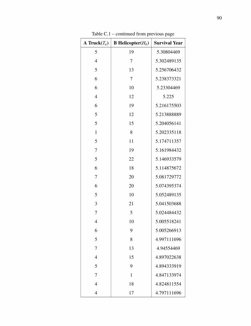
90
Table C.1 – continued from previous page
A Truck(Ta) B Helicopter(Hb) Survival Year
5 19 5.30804469
4 7 5.302489135
5 13 5.256706432
6 7 5.238373321
6 10 5.23304469
4 12 5.225
6 19 5.216175503
5 12 5.213888889
5 15 5.204056141
1 8 5.202335118
5 11 5.174711357
7 19 5.161984432
5 22 5.146933579
6 18 5.114875672
7 20 5.081729772
6 20 5.074395374
5 10 5.052489135
3 21 5.041503688
7 5 5.024484432
4 10 5.005518241
6 9 5.005266913
5 8 4.997111696
7 13 4.94554469
4 15 4.897022638
5 9 4.894333919
7 1 4.847133974
4 18 4.824811554
4 17 4.797111696

91
Table C.1 – continued from previous page
A Truck(Ta) B Helicopter(Hb) Survival Year
4 16 4.797111696
4 4 4.786073797
4 9 4.76940713
7 22 4.768750759
5 14 4.752590395
7 15 4.752436682
5 3 4.741151099
3 22 4.708296019
7 21 4.70383914
4 5 4.691151099
4 11 4.686022863
7 18 4.679861871
7 17 4.661806315
7 16 4.661806315
6 22 4.649889474
6 5 4.641556141
5 6 4.635822468
4 8 4.605266913
5 7 4.552436682
5 5 4.538600246
6 4 4.341378024
6 6 4.219155801
6 2 3.796528537
7 3 3.777489135
6 3 3.674306315
7 2 3.48304469
4 21 2.866567279
4 3 0.002740463

92
Table C.1 – continued from previous page
A Truck(Ta) B Helicopter(Hb) Survival Year
3 4 0.002740463
1 7 0.002691656
4 2 0.002689529
4 1 0.002689529
2 5 0.002689529
3 3 0.002652215
3 2 0.002652215
3 1 0.002652215
2 4 0.002652215
1 6 0.002603407
1 5 0.002566093
2 3 0.002440428
2 2 0.002440428
1 4 0.002354306
2 1 0.002136647
1 3 0.002050525
1 2 0.001746743
1 1 0.001442962
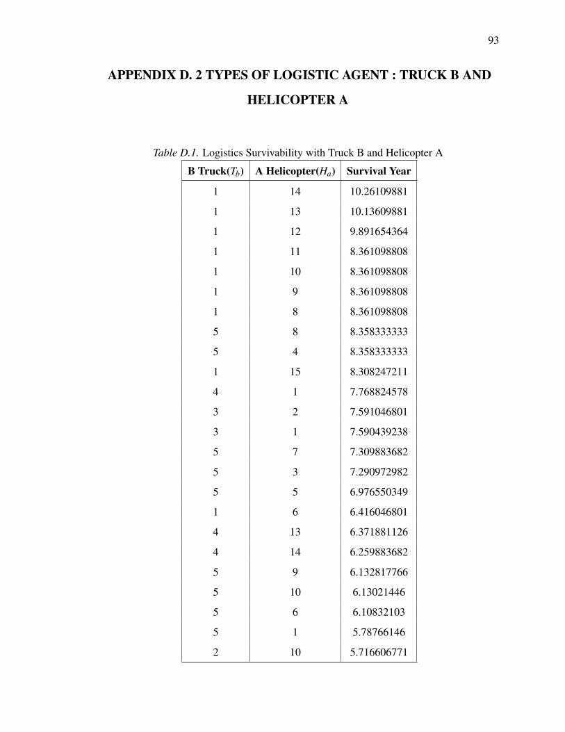
93
APPENDIX D. 2 TYPES OF LOGISTIC AGENT : TRUCK B AND
HELICOPTER A
Table D.1. Logistics Survivability with Truck B and Helicopter A
B Truck(Tb) A Helicopter(Ha) Survival Year
1 14 10.26109881
1 13 10.13609881
1 12 9.891654364
1 11 8.361098808
1 10 8.361098808
1 9 8.361098808
1 8 8.361098808
5 8 8.358333333
5 4 8.358333333
1 15 8.308247211
4 1 7.768824578
3 2 7.591046801
3 1 7.590439238
5 7 7.309883682
5 3 7.290972982
5 5 6.976550349
1 6 6.416046801
4 13 6.371881126
4 14 6.259883682
5 9 6.132817766
5 10 6.13021446
5 6 6.10832103
5 1 5.78766146
2 10 5.716606771

94
Table D.1 – continued from previous page
B Truck(Tb) A Helicopter(Ha) Survival Year
2 11 5.50549566
2 9 5.397033017
2 13 5.291046801
2 6 5.269384549
2 12 5.247162327
3 14 5.169358322
2 15 5.113828993
2 8 5.097162327
2 7 5.097162327
5 13 5.082105904
2 5 5.011051216
5 12 4.993928877
3 15 4.949987697
4 11 4.849380134
4 10 4.749987697
2 14 4.741654364
4 9 4.73332103
5 15 4.527777778
4 15 4.463269023
5 2 4.341046801
3 3 4.335770015
3 13 4.313876586
5 14 4.213547793
5 11 4.077765475
3 6 4.055039988
3 7 3.763547793
3 5 3.6971361
3 11 3.605543252

95
Table D.1 – continued from previous page
B Truck(Tb) A Helicopter(Ha) Survival Year
4 12 3.53332103
3 10 3.530543252
3 8 3.491325571
3 9 3.488876586
3 4 3.441325571
4 2 3.432992237
3 12 3.391654364
4 7 3.174987697
4 8 3.13332103
4 6 3.13332103
4 5 3.13332103
4 4 3.099913878
4 3 3.080469434
2 3 0.002717882
2 2 0.002717882
1 4 0.002479869
2 4 0.002461693
1 7 0.002461693
1 5 0.002401798
2 1 0.002376786
1 3 0.001708113
1 2 0.001426912
1 1 0.001149357

96
APPENDIX E. 2 TYPES OF LOGISTIC AGENT : TRUCK B AND
HELICOPTER B
Table E.1. Logistics Survivability with Truck B and Helicopter B
B Truck(Tb) B Helicopter(Hb) Survival Year
1 21 8.63332103
1 20 8.544432141
1 19 8.513876586
1 17 8.361098808
1 16 8.361098808
1 15 8.361098808
5 14 8.358333333
5 13 8.358333333
5 12 8.358333333
5 11 8.358333333
5 10 8.358333333
5 9 8.358333333
5 8 8.358333333
5 7 8.358333333
5 6 8.358333333
5 5 8.358333333
5 4 8.358333333
5 3 8.358333333
5 2 8.358333333
5 1 8.358333333
1 18 8.35832103
1 22 7.738778363
1 14 6.635693766
5 15 6.552436682

97
Table E.1 – continued from previous page
B Truck(Tb) B Helicopter(Hb) Survival Year
1 13 6.446804877
5 16 6.419444444
1 12 6.416249322
1 11 6.416249322
1 10 6.413775325
1 9 6.413775325
1 8 6.413775325
5 17 6.258333333
5 20 5.866666667
2 13 5.752667252
2 22 5.538600246
2 14 5.352667252
3 22 5.322111696
2 12 5.274711357
3 21 5.216276763
2 16 5.213851574
3 20 5.20544503
3 19 5.174711357
2 21 5.158222808
2 20 5.063778363
4 20 5.058222808
4 16 5.041378024
2 15 5.016556141
2 11 4.92726221
3 18 4.916556141
4 17 4.894333919
4 21 4.872212957
4 19 4.846933579

98
Table E.1 – continued from previous page
B Truck(Tb) B Helicopter(Hb) Survival Year
4 15 4.841629352
2 18 4.838778363
4 22 4.830266913
2 17 4.824889474
4 18 4.822184908
2 9 4.811000585
2 8 4.7717706
2 10 4.766556141
5 18 4.704861871
4 14 4.65804469
2 19 4.633222808
5 19 4.627667252
2 7 4.547111696
5 21 4.507992237
3 17 4.502667252
5 22 4.360417426
3 12 4.358296019
2 6 4.333222808
2 5 4.327667252
4 12 4.277489135
4 13 4.233222808
3 16 4.18304469
4 11 4.163498985
3 15 4.088600246
3 14 4.027667252
4 10 4.016629352
3 11 4.011101846
3 13 3.830266913

99
Table E.1 – continued from previous page
B Truck(Tb) B Helicopter(Hb) Survival Year
3 8 3.80794343
3 9 3.75804469
3 10 3.70544503
4 9 3.561000585
3 7 3.546933579
4 8 3.355266913
4 7 3.221832319
4 5 3.094155801
3 5 3.05544503
3 6 3.019333919
4 6 2.969054541
4 4 2.861000585
4 3 0.011073797
4 2 0.011073797
4 1 0.011073797
3 4 0.011073797
3 3 0.002740463
3 2 0.002740463
3 1 0.002740463
2 4 0.002740463
1 7 0.002691656
1 6 0.002691656
1 5 0.002654341
2 3 0.002528677
2 2 0.002528677
1 4 0.002442555
2 1 0.002224895
1 3 0.002138773

100
Table E.1 – continued from previous page
B Truck(Tb) B Helicopter(Hb) Survival Year
1 2 0.001834992
1 1 0.001531211

101
APPENDIX F. 2 TYPES OF LOGISTIC AGENT : HELICOPTER A
AND HELICOPTER B
Table F.1. Logistics Survivability with Helicopter A and Helicopter B
A Helicopter(Ha) B Helicopter(Hb) Survival Year
7 12 10.12736043
8 11 10.11347154
5 14 10.08486151
14 1 10.07222222
6 13 10.06380277
7 11 10.04639984
13 2 10.04197045
4 15 9.994330881
12 3 9.992817847
3 16 9.991654364
2 17 9.991654364
1 18 9.980543252
11 4 9.979935689
5 13 9.974889474
10 5 9.969596335
13 1 9.948133567
9 6 9.936111111
4 14 9.936000585
12 2 9.9
8 7 9.9
1 17 9.877765475
11 3 9.866654364
3 14 9.85513821
7 8 9.85207179

102
Table F.1 – continued from previous page
A Helicopter(Ha) B Helicopter(Hb) Survival Year
10 4 9.846681441
12 1 9.833333333
9 5 9.831365639
3 15 9.811098808
2 16 9.811098808
6 9 9.802777778
8 6 9.797222222
4 13 9.78332103
11 2 9.778385341
7 7 9.766666667
5 10 9.759383253
10 3 9.731706735
6 12 9.710896287
4 11 9.7
3 13 9.697007398
6 8 9.687262291
9 4 9.667928372
8 5 9.663361018
11 1 9.647981676
5 9 9.626970529
7 6 9.626261706
3 12 9.610693766
6 7 9.582222303
10 2 9.579296685
4 10 9.565040069
5 8 9.5582704
5 12 9.541451843
4 9 9.482501681

103
Table F.1 – continued from previous page
A Helicopter(Ha) B Helicopter(Hb) Survival Year
10 1 9.475
1 16 9.469432141
2 15 9.463876586
2 14 9.463876586
9 3 9.463572804
2 13 9.463572804
3 11 9.463319653
3 10 9.374582655
9 2 9.353587862
8 3 9.340040069
2 12 9.269027099
6 11 9.235946917
7 10 9.135896287
7 3 9.002765475
9 1 8.991654364
8 2 8.991654364
2 11 8.988623435
8 10 8.857814728
6 16 8.744381511
4 18 8.73332103
1 22 8.694358322
4 19 8.644358322
3 20 8.594155801
3 19 8.563778363
8 1 8.561098808
7 2 8.561098808
6 3 8.561098808
1 15 8.561098808

104
Table F.1 – continued from previous page
A Helicopter(Ha) B Helicopter(Hb) Survival Year
1 14 8.561098808
1 13 8.561098808
1 12 8.560693766
2 20 8.555469434
2 21 8.544358322
1 21 8.511024989
2 19 8.446933579
1 20 8.446933579
6 15 8.416580545
1 19 8.341603733
5 17 8.311098808
5 18 8.310693766
5 16 8.297159289
9 8 8.105340731
15 2 8.099835806
15 3 8.074987697
4 12 8.013674065
8 9 8.00832103
4 17 8.005543252
10 8 7.969432141
12 7 7.96912836
9 10 7.949785176
14 4 7.938876586
14 3 7.938876586
11 7 7.938876586
11 8 7.927765475
8 13 7.927691656
11 6 7.919432141

105
Table F.1 – continued from previous page
A Helicopter(Ha) B Helicopter(Hb) Survival Year
12 5 7.90832103
7 14 7.880492622
9 12 7.880469434
13 6 7.861098808
10 7 7.861098808
10 11 7.860822468
9 9 7.855340731
15 1 7.755543252
13 5 7.749785176
3 22 7.744330881
12 6 7.741654364
13 4 7.716654364
14 5 7.688876586
4 21 7.610896287
10 9 7.555543252
11 11 7.547007398
3 18 7.511098808
9 13 7.488876586
13 8 7.461098808
8 14 7.452765475
2 22 7.452765475
12 9 7.430543252
10 12 7.40832103
12 10 7.399987697
7 15 7.391603733
3 21 7.363876586
5 20 7.361048178
14 2 7.352765475
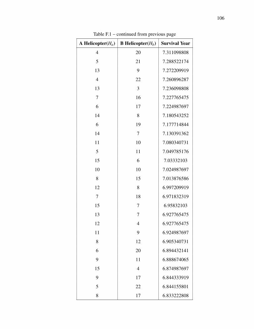
106
Table F.1 – continued from previous page
A Helicopter(Ha) B Helicopter(Hb) Survival Year
4 20 7.311098808
5 21 7.288522174
13 9 7.272209919
4 22 7.260896287
13 3 7.236098808
7 16 7.227765475
6 17 7.224987697
14 8 7.180543252
6 19 7.177714844
14 7 7.130391362
11 10 7.080340731
5 11 7.049785176
15 6 7.03332103
10 10 7.024987697
8 15 7.013876586
12 8 6.997209919
7 18 6.971832319
15 7 6.95832103
13 7 6.927765475
12 4 6.927765475
11 9 6.924987697
8 12 6.905340731
6 20 6.894432141
9 11 6.888674065
15 4 6.874987697
9 17 6.844333919
5 22 6.844155801
8 17 6.833222808

107
Table F.1 – continued from previous page
A Helicopter(Ha) B Helicopter(Hb) Survival Year
7 19 6.824785176
9 16 6.741654364
7 13 6.724785176
6 14 6.702664214
11 12 6.686048178
6 21 6.655492622
11 5 6.613876586
12 11 6.585896287
7 20 6.5832704
15 8 6.569432141
15 5 6.561098808
6 10 6.547007398
10 13 6.53332103
8 18 6.53332103
10 15 6.533118509
13 10 6.527765475
14 6 6.505543252
7 22 6.496832319
14 9 6.480340731
11 14 6.472007398
10 16 6.449633285
9 14 6.413674065
13 12 6.405391362
12 13 6.394432141
10 6 6.380543252
5 19 6.366654364
8 21 6.346832319
15 10 6.33332103

108
Table F.1 – continued from previous page
A Helicopter(Ha) B Helicopter(Hb) Survival Year
14 11 6.302765475
11 15 6.302562954
7 17 6.299987697
6 22 6.2832704
9 20 6.269045276
6 18 6.236098808
12 12 6.199785176
8 19 6.197209919
8 16 6.194432141
7 21 6.19422962
9 7 6.191654364
13 11 6.149785176
12 14 6.127740463
9 18 6.116451843
13 13 6.105543252
10 19 6.105266913
8 20 6.102489135
15 9 6.088876586
14 12 6.080543252
7 9 6.055340731
8 22 6.035899325
14 10 6.027765475
15 11 6.019432141
9 15 6.00832103
11 18 5.994155801
10 17 5.985896287
10 14 5.952765475
9 21 5.910744396
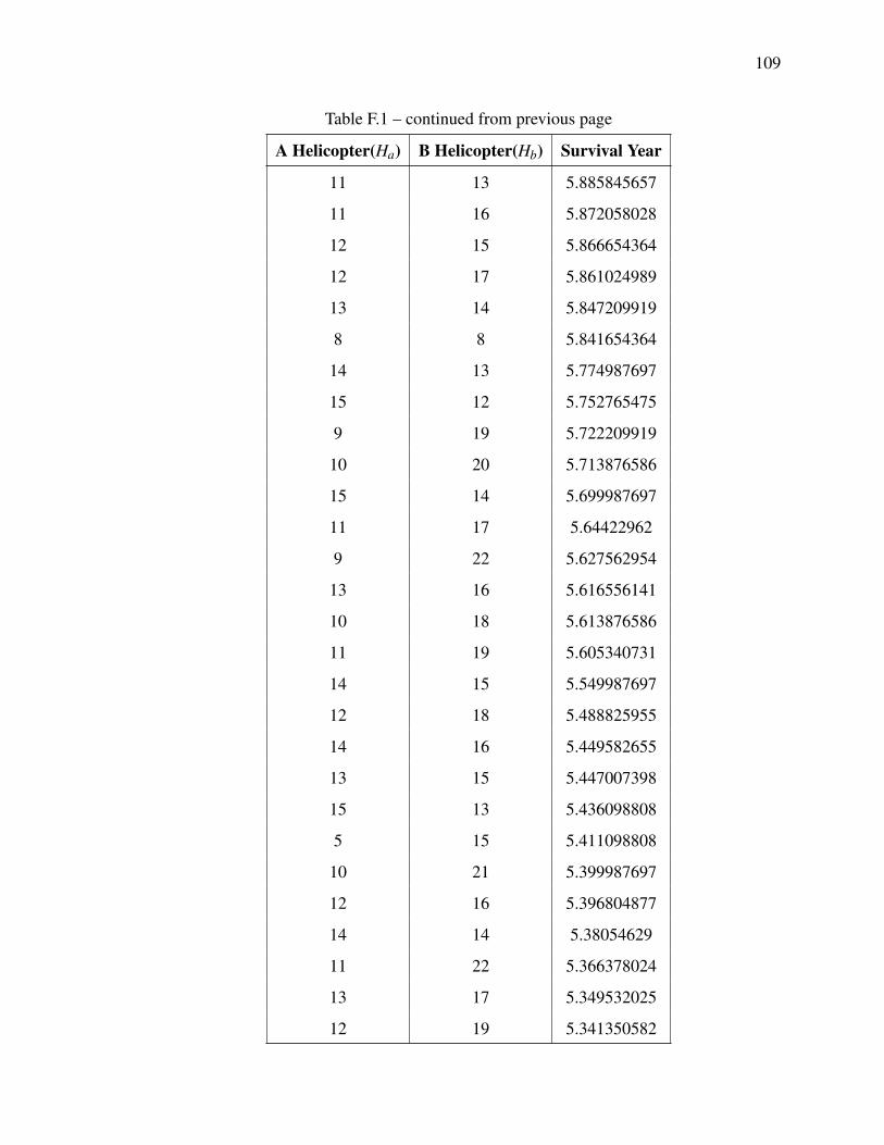
109
Table F.1 – continued from previous page
A Helicopter(Ha) B Helicopter(Hb) Survival Year
11 13 5.885845657
11 16 5.872058028
12 15 5.866654364
12 17 5.861024989
13 14 5.847209919
8 8 5.841654364
14 13 5.774987697
15 12 5.752765475
9 19 5.722209919
10 20 5.713876586
15 14 5.699987697
11 17 5.64422962
9 22 5.627562954
13 16 5.616556141
10 18 5.613876586
11 19 5.605340731
14 15 5.549987697
12 18 5.488825955
14 16 5.449582655
13 15 5.447007398
15 13 5.436098808
5 15 5.411098808
10 21 5.399987697
12 16 5.396804877
14 14 5.38054629
11 22 5.366378024
13 17 5.349532025
12 19 5.341350582
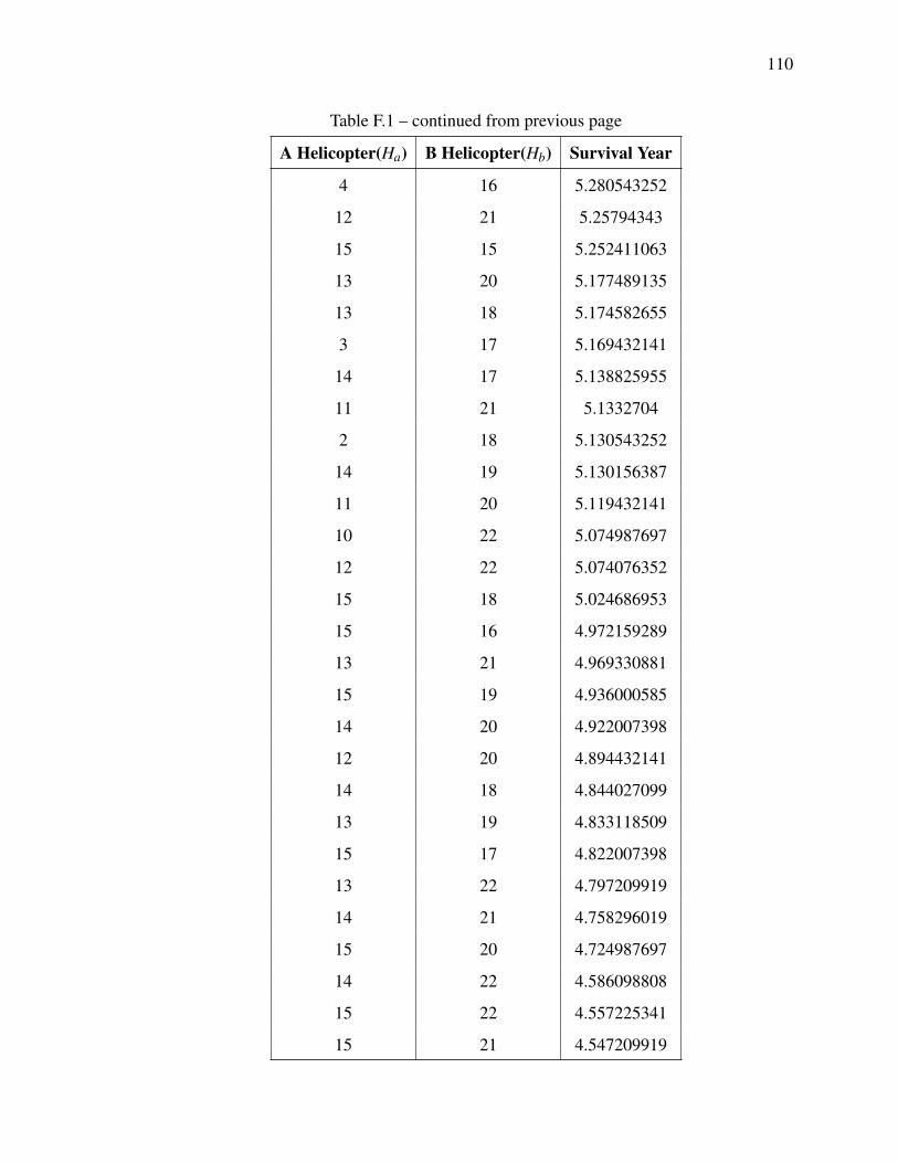
110
Table F.1 – continued from previous page
A Helicopter(Ha) B Helicopter(Hb) Survival Year
4 16 5.280543252
12 21 5.25794343
15 15 5.252411063
13 20 5.177489135
13 18 5.174582655
3 17 5.169432141
14 17 5.138825955
11 21 5.1332704
2 18 5.130543252
14 19 5.130156387
11 20 5.119432141
10 22 5.074987697
12 22 5.074076352
15 18 5.024686953
15 16 4.972159289
13 21 4.969330881
15 19 4.936000585
14 20 4.922007398
12 20 4.894432141
14 18 4.844027099
13 19 4.833118509
15 17 4.822007398
13 22 4.797209919
14 21 4.758296019
15 20 4.724987697
14 22 4.586098808
15 22 4.557225341
15 21 4.547209919

111
Table F.1 – continued from previous page
A Helicopter(Ha) B Helicopter(Hb) Survival Year
8 4 0.002765475
7 5 0.002765475
7 4 0.002765475
6 6 0.002765475
6 5 0.002765475
6 4 0.002765475
5 7 0.002765475
5 6 0.002765475
5 5 0.002765475
5 4 0.002765475
4 7 0.002765475
4 6 0.002765475
3 7 0.002765475
4 5 0.002679353
3 6 0.002679353
2 7 0.002679353
4 8 0.002613584
3 9 0.002613584
3 8 0.002613584
2 10 0.002613584
2 9 0.002613584
2 8 0.002613584
1 11 0.002613584
1 10 0.002613584
1 9 0.002613584
1 8 0.002527462
7 1 0.002461693
6 2 0.002461693

112
Table F.1 – continued from previous page
A Helicopter(Ha) B Helicopter(Hb) Survival Year
6 1 0.002461693
5 3 0.002461693
5 2 0.002461693
4 3 0.002424379
5 1 0.002401798
4 4 0.002309802
3 4 0.002272488
3 5 0.00222368
2 6 0.00222368
1 7 0.00222368
3 3 0.002212592
2 5 0.002186366
1 6 0.002186366
2 4 0.002060702
4 1 0.002011894
4 2 0.002006021
1 5 0.00197458
3 2 0.001860003
2 3 0.001822689
1 4 0.001670798
3 1 0.001556222
2 2 0.001404331
1 3 0.001367017
2 1 0.001215126
1 2 0.001063235
1 1 0.000759

113
APPENDIX G. 3 TYPES OF LOGISTIC AGENT
Table G.1. 3 Types of Logistic agent combinations when LDC allows 10 agents
A Truck(Ta) B Truck(Tb) A Helicopter(Ha) B Helicopter(Hb) Survival Year
1 1 8 0 8.361098808
2 1 7 0 8.360977295
1 5 4 0 7.309414886
3 1 6 0 6.561366531
4 1 5 0 5.730770015
2 5 3 0 5.528586981
3 2 5 0 5.221308124
3 5 2 0 4.9960186
5 4 1 0 4.943569954
1 2 7 0 4.84271446
4 5 1 0 4.804612264
6 3 1 0 4.747091242
2 6 2 0 4.725451774
7 2 1 0 4.553992954
1 6 3 0 4.506291957
3 6 1 0 4.478981127
1 7 2 0 4.328910032
2 7 1 0 4.150641951
4 4 2 0 4.117967307
3 4 3 0 4.052712313
5 3 2 0 3.95880064
4 3 3 0 3.898283057
1 4 5 0 3.896376586
6 1 3 0 3.886586013
4 2 4 0 3.883035658

114
Table G.1 – continued from previous page
A Truck(Ta) B Truck(Tb) A Helicopter(Ha) B Helicopter(Ha) Survival Year
3 3 4 0 3.879641568
7 1 2 0 3.831022863
2 4 4 0 3.825265475
6 2 2 0 3.793522863
1 8 1 0 3.759465527
5 2 3 0 3.691623985
5 1 4 0 3.654709919
2 3 5 0 3.34082103
2 2 6 0 3.244413104
1 3 6 0 3.150821031
0 1 8 1 8.361098808
0 1 6 3 8.269154364
0 1 7 2 8.209633974
0 5 2 3 8.125992059
0 5 1 4 7.468110601
0 1 1 8 6.413775325
0 1 5 4 6.344588406
0 1 4 5 5.152280113
0 1 3 6 4.824653537
0 7 1 2 4.542613108
0 7 2 1 4.5147281
0 1 2 7 4.491910512
0 2 6 2 4.306879486
0 2 7 1 4.242440105
0 6 3 1 4.05094154
0 2 5 3 4.043515774
0 2 1 7 4.032909285
0 8 1 1 3.993750759
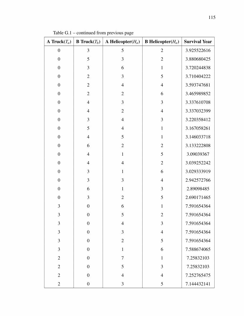
115
Table G.1 – continued from previous page
A Truck(Ta) B Truck(Tb) A Helicopter(Ha) B Helicopter(Ha) Survival Year
0 3 5 2 3.925522616
0 5 3 2 3.880680425
0 3 6 1 3.720244838
0 2 3 5 3.710404222
0 2 4 4 3.593747681
0 2 2 6 3.465989852
0 4 3 3 3.337610708
0 4 2 4 3.337032399
0 3 4 3 3.220358412
0 5 4 1 3.167058261
0 4 5 1 3.146033718
0 6 2 2 3.133222808
0 4 1 5 3.09039367
0 4 4 2 3.039252242
0 3 1 6 3.029333919
0 3 3 4 2.942572766
0 6 1 3 2.89098485
0 3 2 5 2.690171465
3 0 6 1 7.591654364
3 0 5 2 7.591654364
3 0 4 3 7.591654364
3 0 3 4 7.591654364
3 0 2 5 7.591654364
3 0 1 6 7.588674065
2 0 7 1 7.25832103
2 0 5 3 7.25832103
2 0 4 4 7.252765475
2 0 3 5 7.144432141

116
Table G.1 – continued from previous page
A Truck(Ta) B Truck(Tb) A Helicopter(Ha) B Helicopter(Ha) Survival Year
2 0 2 6 7.097209919
2 0 6 2 7.074380134
2 0 1 7 7.052461693
1 0 8 1 6.416654364
1 0 7 2 6.402765475
1 0 6 3 6.361098808
1 0 5 4 6.277157912
1 0 4 5 6.241654364
1 0 3 6 6.169432141
1 0 2 7 6.060491245
4 0 3 3 5.888373321
4 0 4 2 5.885770015
7 0 1 2 5.708247211
5 0 2 3 5.577436682
5 0 1 4 5.577436682
4 0 2 4 5.536073797
1 0 1 8 5.513446229
4 0 1 5 5.371706654
4 0 5 1 5.130469434
7 0 2 1 5.122133974
6 0 3 1 4.816580545
5 0 3 2 4.430266913
5 0 4 1 4.3971361
6 0 2 2 3.691151099
6 0 1 3 3.388802767
2 1 0 7 6.018851575
3 1 0 6 5.975770886
6 1 0 3 5.915228029

117
Table G.1 – continued from previous page
A Truck(Ta) B Truck(Tb) A Helicopter(Ha) B Helicopter(Ha) Survival Year
2 5 0 3 5.580975184
5 4 0 1 5.422903229
7 1 0 2 5.382663424
4 4 0 2 5.296754146
6 3 0 1 5.161535686
5 3 0 2 5.159523225
4 5 0 1 5.144955688
7 2 0 1 5.091813464
3 5 0 2 5.055630438
2 4 0 4 4.982140981
6 2 0 2 4.892894405
4 1 0 5 4.796207116
2 6 0 2 4.689206654
3 6 0 1 4.621763664
3 4 0 3 4.566752728
1 7 0 2 4.279484432
2 7 0 1 4.164401996
5 1 0 4 4.053437034
2 2 0 6 4.027725821
1 2 0 7 3.918700777
4 2 0 4 3.632223924
5 2 0 3 3.556072673
3 2 0 5 3.515601295
1 6 0 3 3.404808466
4 3 0 3 3.401798295
3 3 0 4 3.360284724
1 4 0 5 3.175641435
1 3 0 6 3.133375903

118
Table G.1 – continued from previous page
A Truck(Ta) B Truck(Tb) A Helicopter(Ha) B Helicopter(Ha) Survival Year
2 3 0 5 3.086171493
1 5 0 4 2.969576073

119
APPENDIX H. 4 TYPES OF LOGISTIC AGENT
Table H.1. 4 Types of Logistic agent combinations when LDC allows 10 agents
A Truck(Ta) B Truck(Tb) A Helicopter(Ha) B Helicopter(Hb) Survival Year
1 1 7 1 8.361098808
2 1 6 1 8.360451799
2 1 5 2 8.356256881
2 1 4 3 8.355722808
2 1 3 4 8.351833919
1 1 5 3 8.35042174
2 1 2 5 8.344611696
1 1 4 4 8.301274637
1 5 3 1 8.186158729
1 1 6 2 8.133866764
3 1 4 2 6.354658904
1 1 2 6 6.28044503
1 1 3 5 6.261267933
3 1 3 3 6.248425663
1 1 1 7 6.08044503
3 1 5 1 5.848790676
2 4 1 3 5.535039401
4 1 4 1 5.534936682
6 1 2 1 5.388748755
2 1 1 6 5.381073797
7 1 1 1 5.305781751
2 5 2 1 5.301984432
2 4 2 2 5.289081537
3 2 4 1 5.188512899
4 4 1 1 5.130876855

120
Table H.1 – continued from previous page
A Truck(Ta) B Truck(Tb) A Helicopter(Ha) B Helicopter(Ha) Survival Year
5 3 1 1 4.967689529
3 5 1 1 4.95820213
4 1 2 3 4.91314752
4 1 3 2 4.8405342
1 2 6 1 4.836881126
1 6 2 1 4.819797104
2 6 1 1 4.813107477
1 6 1 2 4.787119838
6 2 1 1 4.747881479
3 1 2 4 4.618188754
2 3 3 2 4.608252679
5 2 2 1 4.53451395
1 5 2 2 4.530709451
1 2 5 2 4.520773438
1 4 1 4 4.481499537
3 4 1 2 4.448160897
2 5 1 2 4.428577553
5 1 3 1 4.4096361
1 5 1 3 4.385886029
1 7 1 1 4.373147885
4 3 2 1 4.348341657
4 2 3 1 4.305407614