discovery of a major coal deposit in china with the use of ... · discovery of a major coal deposit...

Discovery of a Major Coal Deposit in China with the Use of a Modified CSAMT Method

Guoqiang Xue1,*, Shu Yan2, L.-J. Gelius3, Weiying Chen1, Nannan Zhou1 and Hai Li1

1Key Laboratory of Mineral Resources, Institute of Geology and Geophysics, Chinese Academy of Sciences,

19 Beitucheng Western Road, Beijing 100029, China2School of Computer Science and Telecommunication Engineering, Jiangsu University, 301 Xuefu Road,

Zhenjiang 212013, China3Department of Geosciences, University of Oslo, 1072 Blindern, 0316 Oslo, Norway

*Email: [email protected]; Tel.: +86-10-82998193

ABSTRACT

Conventional use of the controlled-source audio-frequency magneto-telluric (CSAMT)

method is based on calculating the apparent or Cagniard resistivity from the amplitude ratio of

the horizontal electric and magnetic field components. However, direct comparison between

these two components shows that the electric field is more sensitive to the underground medium

resistivity than its magnetic counterpart. Thus, use of the electric component only should

provide adequate information about the electric properties of the subsurface. The measurementstypically belong to the far-field zone, but show a non-dipolar characteristic because of the

source. In this paper, we therefore propose a simplified CSAMT technique based on measuring

the electric field component only. As part of this new formulation, a related theoretical model

for the electric field component accounting for the non-dipolar nature of the transmitter

antenna is introduced. This is accompanied with a new apparent resistivity definition, including

a procedure to transform it into pseudo-phase data, thus removing the static shifts.

The potential of this modified CSAMT method is demonstrated using a field case from the

Shanxi province in China. Until recently, it has been thought that no coal deposits exist in thisregion. However, application of the single-component CSAMT technique as advocated for here,

revealed a major coal deposit, which was verified later by drilling.

Introduction

The development of the controlled-source audio

frequency magneto-telluric (CSAMT) method was

inspired by the magneto-telluric (MT) technique (Gold-

stein, 1971; Goldstein and Strangway, 1975). Because of

the many advantages of CSAMT regarding information

content, signal strength, work efficiency and detection

accuracy, the technique has received increasing atten-

tion. CSAMT has been successfully applied within

metaliferous mining (Boerner, 1993; Chen, 1993),

petroleum exploration (Ranganayaki, 1992), deep sea

environmental investigations (Di, 2002), groundwater

studies (Christensen, 2000) and geothermal exploration

(Sandberg and Hohmann, 1982; Batrel and Jacobson,

1987; Wannamaker, 1997). Bartel and Jacobson, 1987)

used CSAMT surveying to identify faults and fissure-

type water storage structures in mountainous karstic

terrain. The CSAMT method has also proven very

useful when searching for certain ore structures, because

of its ability to delineate the abnormal shape and

position of a body (Boschetto and Hohmann, 1991). In

the prediction of geology in advance of mining, it is

important to locate faults and karst caves. CSAMT has

been successful in preventing and controlling disasters

by detecting the distribution of water-bearing ore zones

in the roof and floor ahead of extraction (Chen and

Yan, 2005).

To reduce field data costs, in a practical CSAMT

survey six electrical field points will share one magnetic-

field recording station, as shown in Fig. 1. Apparent

resistivities are then estimated from the ratio between

the measured horizontal components of the electric and

magnetic fields, Ex and Hy, respectively (Goldstein and

Strangway, 1975; Zong et al., 1986, 1991). This type of

acquisition inherently acknowledges the fact that the

electric field component is the most important informa-

tion carrier of the subsurface. In this paper, we propose

to use the electric field component only, and present a

modified theoretical model to analyze the data and

provide apparent resistivity maps (referred to as the

single-component resistivity formula). This modified or

single-component CSAMT technique was applied in the

Shanxi region in China, an area that was earlier assumed

47

JEEG, March 2015, Volume 20, Issue 1, pp. 47–56 DOI: 10.2113/JEEG20.1.47

to be free of coal deposits. However, use of the method

revealed a major coal deposit at depth, between 600 m

and 800 m. This prospect was later verified by drilling.

Methodology

Single-component Resistivity Formula

A simple analysis supporting the idea of using the

electric component only is given in Appendix A. In thefollowing, we proceed to analyze this field component

only. In the case of far field, the apparent resistivity

effectively normalizes out the effects of current strength,

dipole length, frequency, source-receiver distance and

orientation relative to the source. Thus, it can be defined

through a single component of the electric or magnetic

field in the far-field zone (Kaufman and Keller, 1983).

When using the inline electric field component, theapparent resistivity is given by:

rEx(v)~

4p:r3

I :l

Ex(v)

3 cos 2a{1

��2

, ð1Þ

where I is the current, l is the length of the source, a is

the angle between the observation point vector and the

source line direction, and r is the distance from the

observation point and the center of the transmittingantenna. The x-component of the electric field was

chosen because of its larger magnitude since it is

oriented parallel to the source orientation.

In this work, we propose to further refine the

expression in Eq. (1) by taking into account the non-

dipole nature of the transmitter antenna. A finite-length

antenna with length AB is then subdivided into many

small segments as shown in Fig. 2. The reader is referred

to Appendix B for the necessary details of the

derivation; we only state the main result here:

rEx

i (v)~p:r3

MN:l: 4r2zl2

r(8r2zl2):DVi(v)

I, ð2Þ

where DVi(v) is the observed voltage difference between

two neighboring receiver (MN) electrodes.

The single-component resistivity formula, as given

by Eq. (2), is derived for a uniform half-space. Thus, by

using this formula to estimate the apparent resistivity in

the case of a layered Earth model, a volume-averaged

resistivity estimate should be obtained. We consider a

simple synthetic case to verify this assumption. To

further test the validity of Eq. (2), we also compare it

with the resistivity estimate obtained employing the

standard two-component formula according to Cag-

niard (1950, 1953):

rEx=Hyv (v)~

1

vm0

Ex(v)

Hy(v)

��2

: ð3Þ

Note that Eq. (3) is derived assuming a homogenous

Earth.

Figure 1. Typical acquisition layout of standard

CSAMT survey.

Figure 2. Sketch indicating a small element along the

current line AB for which the electric field contribution is

computed at receiver position r. The total contribution is

obtained by summing over all such incremental responses.

48

Journal of Environmental and Engineering Geophysics

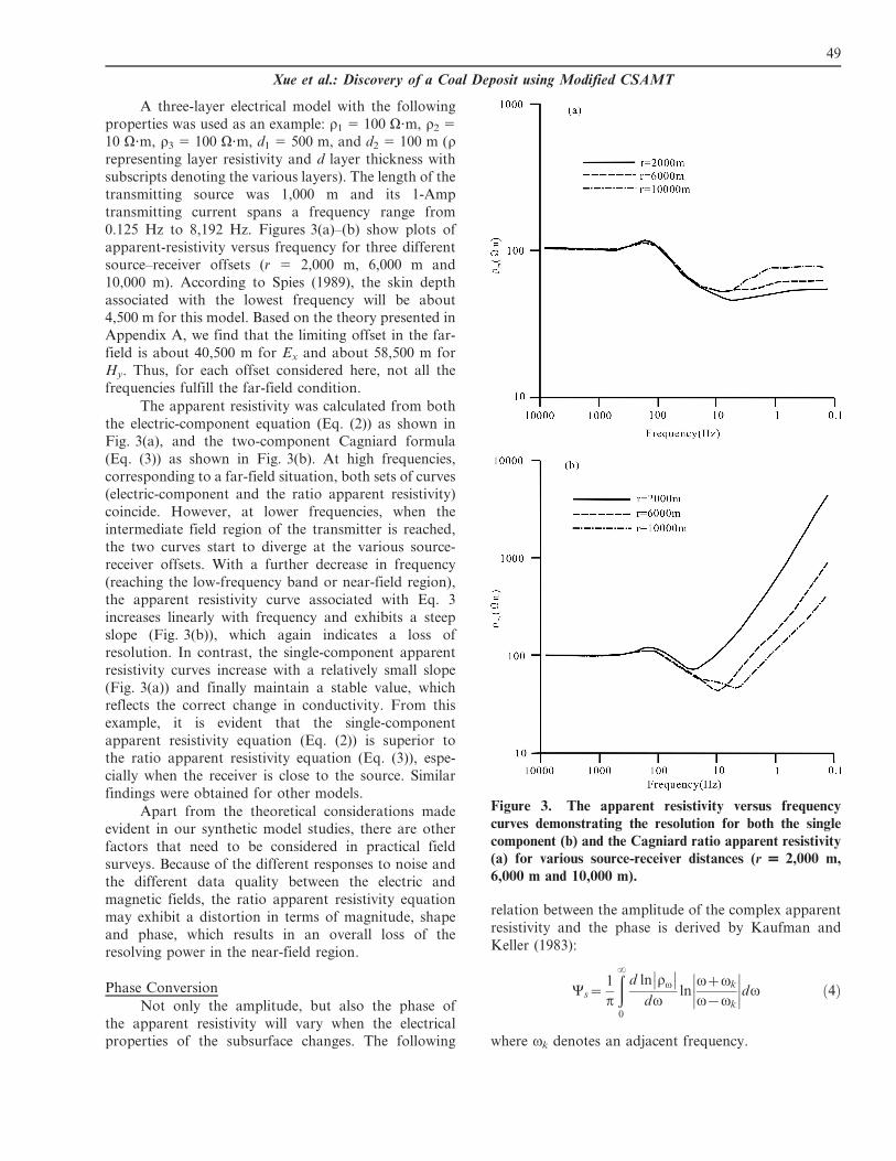
A three-layer electrical model with the following

properties was used as an example: r1 5 100 V?m, r2 5

10 V?m, r3 5 100 V?m, d1 5 500 m, and d2 5 100 m (rrepresenting layer resistivity and d layer thickness with

subscripts denoting the various layers). The length of the

transmitting source was 1,000 m and its 1-Amp

transmitting current spans a frequency range from

0.125 Hz to 8,192 Hz. Figures 3(a)–(b) show plots of

apparent-resistivity versus frequency for three different

source–receiver offsets (r 5 2,000 m, 6,000 m and

10,000 m). According to Spies (1989), the skin depth

associated with the lowest frequency will be about

4,500 m for this model. Based on the theory presented in

Appendix A, we find that the limiting offset in the far-

field is about 40,500 m for Ex and about 58,500 m for

Hy. Thus, for each offset considered here, not all the

frequencies fulfill the far-field condition.

The apparent resistivity was calculated from both

the electric-component equation (Eq. (2)) as shown in

Fig. 3(a), and the two-component Cagniard formula

(Eq. (3)) as shown in Fig. 3(b). At high frequencies,

corresponding to a far-field situation, both sets of curves

(electric-component and the ratio apparent resistivity)

coincide. However, at lower frequencies, when the

intermediate field region of the transmitter is reached,

the two curves start to diverge at the various source-

receiver offsets. With a further decrease in frequency

(reaching the low-frequency band or near-field region),

the apparent resistivity curve associated with Eq. 3

increases linearly with frequency and exhibits a steep

slope (Fig. 3(b)), which again indicates a loss of

resolution. In contrast, the single-component apparent

resistivity curves increase with a relatively small slope

(Fig. 3(a)) and finally maintain a stable value, which

reflects the correct change in conductivity. From this

example, it is evident that the single-component

apparent resistivity equation (Eq. (2)) is superior to

the ratio apparent resistivity equation (Eq. (3)), espe-

cially when the receiver is close to the source. Similar

findings were obtained for other models.

Apart from the theoretical considerations made

evident in our synthetic model studies, there are other

factors that need to be considered in practical field

surveys. Because of the different responses to noise and

the different data quality between the electric and

magnetic fields, the ratio apparent resistivity equation

may exhibit a distortion in terms of magnitude, shape

and phase, which results in an overall loss of the

resolving power in the near-field region.

Phase Conversion

Not only the amplitude, but also the phase of

the apparent resistivity will vary when the electrical

properties of the subsurface changes. The following

relation between the amplitude of the complex apparent

resistivity and the phase is derived by Kaufman and

Keller (1983):

Ys~1

p

ð?

0

d ln rv��

dvln

vzvk

v{vk

��dv ð4Þ

where vk denotes an adjacent frequency.

Figure 3. The apparent resistivity versus frequency

curves demonstrating the resolution for both the single

component (b) and the Cagniard ratio apparent resistivity(a) for various source-receiver distances (r = 2,000 m,

6,000 m and 10,000 m).

49

Xue et al.: Discovery of a Coal Deposit using Modified CSAMT

From Eq. (4), it follows that the phase curve is

related to the slope of the apparent resistivity curve. It is

therefore possible to remove the static shift between

apparent-resistivity curves according to the phase curve.

Equation (4) can be further simplified as follows

(Kaufman and Keller, 1983):

Ys & 450+450 ln rs

lnvð5Þ

According to Eq. (5), the apparent phase is a function of

the rate of change of the frequency. Therefore, it is

possible to obtain the apparent phase from the

knowledge of the apparent resistivity. The phase

conversion method using the single-component appar-

ent resistivity is an efficient way to solve the static shift

problem. For special cases, like a geological stratum

consisting of an embedded thin layer, it is not possible to

use the amplitude curve of the apparent resistivity.

However, the alternative use of the phase curve may

distinguish the thin layer. Also, when the geological

stratum is buried in a highly resistive basement, it is also

not possible to use the amplitude curve for distinguish-

ing the basement. This is because of the limited electrode

separation and no significant difference in electrical

properties. However, again the converted phase curve

shows a better performance under such conditions.

To demonstrate the feasibility of the converted

phase approach, a simple synthetic model with the

following electrical properties was considered: r1 5 10

V?m, r2 5 400 V?m, r3 5 10 V?m, d1 5 10 m, d2 5

100 m, and r 5 2,000 m. Figure 4 shows a plot of the

converted phase curve (asterisk line) together with the

theoretical apparent phase curve (solid line) for 26

sampled frequencies between 0.125 Hz and 4,096 Hz. It

is clear that no visible differences appear between the

two curves. This supports the use of the converted phase

curve since it exhibits the same resolving power as its

theoretical counterpart. However, a basic condition is

that measurements are carried out for a sufficient

recording time.

Case Study from Coal Exploration

Survey Environment and Electromagnetic Disturbances

The case study is taken from the Yangqu County,

located in the northern part of Taiyuan City in the

Shanxi Province in China. From earlier investigations,

this particular region was considered to contain no

significant coal deposits. This conclusion was partly

based on the finding of Cenozoic gray-green rock in one

of the drilled holes, which lead to the wrong conclusionthat this stratum belongs to the Benxi group. However,

because of energy shortages, the authors were invited to

conduct a modified CSAMT survey in this region to

further assess its coal potential.

The survey area is located in the northern part of

the Taiyuan basin in the piedmont hills, which are fully

covered by loess with a thickness between 300–400 m

and in the center of a syncline with preserved coalseams. The geological strata are from the Ordovician,

Carboniferous-Permian and Cenozoic ages. The Car-

boniferous strata mainly contain the coal seams, which

have an average thickness of 6.7 m as revealed by

borehole records.

The survey region is shown in Fig. 5, where the

upper left corner of the map is a picture of the area, the

lower left map shows the location within China, and thelower central map is of Shanxi Province. The main part

of the figure describes the outlay of the survey, including

22 south to north directed survey lines at 100-m line

Figure 4. Comparison between true (calculated frommodel) and converted phase curves.

Figure 5. The lower left panel is a map of China; the

lower middle panel shows the Shanxi Province and the

location of Yangqu County; the upper left panel is a photo

of the field area; and the middle panel shows the outlay of

the survey.

50


interval and observation points at every 50 m. The

survey area covered a total of 15 km2. From previous

drilling and well logs, the main electrical parameters for

the survey region were obtained (see Table 1). It can be

seen from Table 1 that the shallow strata show low

resistivity, the coal seam has a relatively high resistivity,

and the basement of the coal layers shows the highest

resistivity. These observations can be used to determine

the lower depth of the coal seam.

As advocated for in this paper, the CSAMT survey

was carried out measuring only a single component (Ex)

of the electrical sensors. An equatorial dipole array was

exploited with r 5 3,000 m, AB 5 1,000 m and MN 5

200 m. The frequencies used are listed in Table 2.

Data Processing and Interpretation

To analyze the processed data properly, modeling

of some typical strata was performed prior to the field

surveys. The model results are shown in Fig. 6, which

gives the characteristic shape of the apparent resistivity

curve for two different scenarios:

N H curve (Q + N strata overlying O2 strata) shown in

Fig. 6(a)

N HA curve (same as H, but with a layer of P + C in

between) shown in Fig. 6(b).

At first glance, these two curves look very similar inshape, but there are obvious differences: 1) the ratio

between the maximum and minimum value is different,

with that in Fig. 6(a) being the largest, which again

means that a large geo-electric difference exists between

the basement and the overburden; and 2) the frequency

number corresponding to the minimum value of

resistivity is different, with that of Fig. 6(a) representing

the largest frequency (see Table 2 for conversion), whichagain corresponds to a shallow burial depth of the

basement. Correspondingly, the burial depth of the

basement in Fig. 6(b) is deeper, which may represent

the case of a possible coal deposit.

In general, if the basement of the coal seam is the

Ordovician grey rock, then it can be regarded as the

standard electrical basement stratum because of its wide

distribution and high resistivity. However, if the

geological section contains the Carboniferous-Permian

coal seams, then the CSAMT apparent resistivitysounding curves often exhibit an HA pattern (Fig. 6(b)).

Conversely, when the sounding curve displays an H type

pattern (Fig. 6(a)) then coal is absent. Such features can

be regarded as the basic principle with which to

recognize the presence of coal in the stratigraphic

section. In this survey region, two types of sounding

curves can be recognized: one is the H pattern (Fig. 6(a))

and the other is the HA pattern (Fig. 6(b)). The formerindicates the presence of coal beneath the Cenozoic; the

latter indicates that the thick Cenozoic is directly in

contact with the Ordovician limestone and there are no

embedded Permo-Carboniferous strata.

Now, let us turn to the actual measurements

obtained. Figure 7(a) shows the ensemble of apparent

resistivity versus frequency sounding curves for line 14.

In this figure, the curves corresponding to small station

numbers (2–14) exhibit the H-type pattern, whichindicates that there are no subsurface buried coal seams;

however, at larger station numbers (18–42) the HA

Table 1. Main electrical parameters for the surveyregion.

Geological age Rock type Resistivity

Quaternary Loess, clay, silt 16–50 V?m

Tertiary Sand clay 40–100 V?m

Carboniferous

Permian

Mudstone, pink

sandstone, coal, thin

limestone

70–360 V?m

Ordovician Thick limestone .500 V?m

Table 2. Frequency conversion table.

Sample Point No. 1 2 3 4 5 6 7 8

Frequency 2,844 1,280 512 426.67 341.33 256 213.33 170.67

Sample Point No. 9 10 11 12 13 14 15 16

Frequency 128 106.67 85.333 64 53.33 42.667 32 26.667

Sample Point No. 17 18 19 20 21 22 23 24

Frequency 21.333 16 13.33 10.667 8 6.667 5.333 4

Sample Point No. 25 26 27 28 29 30 31 32

Frequency 3.333 2.6667 2 1.6667 1.333 1 0.833 0.6667

Sample Point No. 33 34 35 36 37 38 39 40

Frequency 0.5 0.41667 0.3333 0.25 0.20833 0.15 0.125 0.01

Sample Point No. 41

Frequency 0.08

51


pattern is observed, which indicates that there are coal

seams present. Figure 7(b) shows the apparent resistivity

map along the same line after depth conversion. The

apparent resistivity was transformed into depth accord-

ing to the skin depth equation:

d~503|

ffiffiffir

f

rð6Þ

Correspondingly, Fig. 7(c) represents the sectional map

of the converted phase. From the extension and

variation of the contour map, the coal fault can be

inferred to be of fold type. Combined with drilling

results available in the survey region, the final inter-

preted geological sectional map is as shown in Fig. 7(d).

Two coal bearing strata exist following a synclinal

structure and located in a deeply buried rift basin, which

is cut by two faults, labeled as F4 and F5 in the figure.

Later Drilling Test

Based on the geo-electrical mapping results (see

Fig. 7), a drill hole was selected near station 18 of line 14

(see Fig. 7(c)). The total drilling depth was 678.37 m.

Analyses of the borehole cores verified that two coal

seams are present. The depth of the upper coal stratum

is 566.91 m with a thickness of 5.18 m, while the depth

of the lower coal stratum is 652.52 m with a thickness of

9.65 m. Both coal seams have a small dip (less than 10u).A geological log of the borehole is presented in

Fig. 8(a). The deep sounding curve near the drill hole

is shown in Fig. 8(b).

The CSAMT survey shows that the region

contains a coal bearing structure, and is able to

approximately delineate the boundaries. Subsequent

drilling verified our prediction of the coal structure,

Figure 6. The H (a) and HA (b) pattern of the apparent

resistivity curves. The abbreviations at the bottom are Q +N: Cenozoic Quaternary and Tertiary stratum; P + C:

Permian + Carboniferous strata; and O2: Ordovician strata.

Figure 7. a) Map of apparent resistivity versus frequen-cy (line 14), b) resistivity map after depth conversion, c)

corresponding phase contour map and d) final geological

interpreted section (same abbreviations as used in Fig. 6).

52


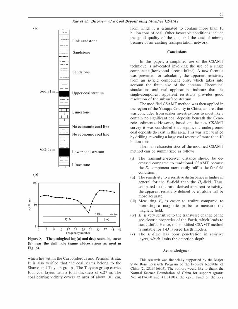
which lies within the Carboniferous and Permian strata.

It is also verified that the coal seams belong to the

Shanxi and Taiyuan groups. The Taiyuan group carriesfour coal layers with a total thickness of 6.27 m. The

coal bearing vicinity covers an area of about 101 km,

from which it is estimated to contain more than 10

billion tons of coal. Other favorable conditions include

the good quality of the coal and the ease of mining

because of an existing transportation network.

Conclusions

In this paper, a simplified use of the CSAMT

technique is advocated involving the use of a single

component (horizontal electric inline). A new formula

was presented for calculating the apparent resistivity

from an E-field component only, which takes into

account the finite size of the antenna. Theoretical

simulations and real applications indicate that the

single-component apparent resistivity provides good

resolution of the subsurface stratum.

The modified CSAMT method was then applied in

the region of the Yanqqu County in China, an area that

was concluded from earlier investigations to most likely

contain no significant coal deposits beneath the Ceno-

zoic sediments. However, based on the new CSAMT

survey it was concluded that significant underground

coal deposits do exist in this area. This was later verified

by drilling, revealing a large coal reserve of more than 10

billion tons.

The main characteristics of the modified CSAMT

method can be summarized as follows:

(i) The transmitter-receiver distance should be de-

creased compared to traditional CSAMT because

the Ex-component more easily fulfills the far-field

condition.

(ii) The sensitivity to a resistive disturbance is higher in

general for the Ex-field than the Hy-field. Thus,

compared to the ratio-derived apparent resistivity,

the apparent resistivity defined by Ex alone will be

more accurate.

(iii) Measuring Ex is easier to realize compared to

mounting a magnetic probe to measure the

magnetic field.

(iv) Ex is very sensitive to the transverse change of the

geo-electric properties of the Earth, which leads to

static shifts. Hence, this modified CSAMT method

is suitable for 1-D layered Earth models.

(v) The Ex-field has poor penetration in resistive

layers, which limits the detection depth.

Acknowledgment

This research was financially supported by the Major

State Basic Research Program of the People’s Republic of

China (2012CB416605). The authors would like to thank the

Natural Science Foundation of China for support (grants

No. 41174090 and 41174108), the open Fund of the Key

Figure 8. The geological log (a) and deep sounding curve

(b) near the drill hole (same abbreviations as used in

Fig. 6).

53


Laboratory of Mineral Resources, Chinese Academy of

Sciences, as well as Major National Research Equipment

Development Project (ZDYZ2012-1-05-04).

References

Bartel, L.C., and Jacobson, R.D., 1987, Results of a

controlled-source audio frequency magnetotelluric sur-

vey at the Puhimau thermal area, Kilauea Volcano,

Hawaii: Geophysics, 5, 665–77.

Boschetto, N.B., and Hohmann, G.W., 1991, Controlled

source audio frequency magnetotelluric responses of

three-dimensional bodies: Geophysics, 56, 255–64.

Boerner, D.E., Wright, J.A., Thurlow, J.G., and Reed, L.E.,

1993, Tensor CSAMT studies at the Buchan’s mine in

central New Foundland: Geophysics, 58, 12–9.

Cagniard, L., 1950, Procedure for geophysical prospecting:

French patent No. 1025683.

Chen, C.S., 1993, Application of CSAMT method for gold

copper deposits in Chinkuashih area, Northern Taiwan:

TAO, 4, 339–50.

Cagniard, L., 1953, Principle of magneto-telluric method, a

new method of geophysical prospecting: Ann. de

Geophys., 9, 95–125.

Chen, M.S., and Yan, S., 2005, Analytical study on field zones,

record rules, shadow and source overprint effects in

CSAMT exploration: Chinese J. Geophys. (in Chinese),

48, 951–958.

Christensen, N.B., 2000, Difficulties in determining electrical

anisotropy in subsurface investigations: Geophys.

Prosp., 48, 1–19.

Di, Q.Y., Wang, M.Y., Shi, K.F., and Zhang, G.L., 2002,

CSAMT research survey for preventing water-bursting

disaster in mining: Proceeding of the SEGJ Conference,

Tokyo.

Goldstein, M.A., 1971, Magneto-telluric experiments employ-

ing an artificial dipole source: Ph.D. thesis, University of

Toronto, Toronto.

Goldstein, M.A., and Strangway, D.W., 1975, Audio-frequen-

cy magnetotellurics with a ground electric dipole source:

Geophysics, 40, 669–83.

Hosseini, K., Montazeri, A., Alikhanian, H., and Kahaei,

M.H., 2008, New classes of LMS and LMF adaptive

algorithms. Information and Communication Technol-

ogies: From theory to applications: ICTTA, 3rd

International Conference on 05/2008, doi: 10.1109/

ICTTA.2008.4530045.

Kaufman, A., and Keller, G.V., 1983, Frequency and transient

sounding, Elsevier Science Publishers, B.V. 110–115,

213–226.

Nabighian, M.N., 1979, Quasi-static transient response of a

conducting half-space: Geophysics, 44, 1700–1705.

Ranganayaki, R.P., Fryer, S.M., and Bartel, L.C., 1992,

CSAMT surveys in a heavy oil field to monitor steam

drive enhanced oil recovery process: in Expanded

Abstracts, 62nd Annual International Meeting, Society

of Exploration Geophysicists, 1384.

Routh, P.S., and Oldenburg, D.W., 1999, Inversion of

controlled source audio frequency magnetotellurics data

for a horizontally layered Earth: Geophysics, 64,

1689–97.

Sandberg, S.K., and Hohmann, G.W., 1982, Controlled-

source audio-magnetotellurics in geothermal explora-

tion: Geophysics, 47, 100–116.

Spies, B.R., 1989, Depth of investigation in electromagnetic

sounding methods: Geophysics, 54, 872–888.

Tikhonov, A.N., 1950, On determining the electrical charac-

teristics of the deep layers of the Earth’s crust: Doklady,

73, 295–297.

Wannamaker, P.E., 1997, Tensor CSAM T survey over the

Sulphur Springs thermal area, Valles Caldera, New

Mexico, USA, Part E: Implications for structure of the

western equations: Geophysics, 62, 451–65.

Zonge, K.L., Ostrander, A.G., and Emer, D.F., 1986, Con-

trolled-source audio-frequency magnetotelluric measure-

ments: in Magnetotelluric methods, Vozoff, K. (ed.), Soc.

Expl. Geophys., Geophysics Reprint Series, 5, 749–763.

Zonge, K.L., and Hughes, L.J., 1991, Controlled source

audiomagnetotellurics: in Electromagnetic Methods in

Applied Geophysics, Volume 2, Application, Part B:

Nabighian, M.N. (ed.), Society of Exploration Geo-

physicists, Tulsa, OK, 713–809.

APPENDIX A

ELECTRIC FIELD COMPONENT VERSUS

MAGNETIC FIELD COMPONENT IN CSAMT

Let I ,L,r represent current, wire length and

separation, respectively. The electric field Ew(v) and

magnetic field Hr(v) responses in case of the CSAMT

method can then be written as (Cagniard, 1950, 1953):

Ew(v)~I :l

2ps

1

r31{3 sin2 wze{ikr 1zikrð Þ� �

ðA-1Þ

Hr(v)~I :l

4ps

1

r2sinw 6I1

ikr

2

� �K1

ikr

2

� ��

zikr I1ikr

2

� �K0

ikr

2

� �{I0

ikr

2

� �K1

ikr

2

� � �:

For the far-field, Eqs. (A-1) and (A-2) can be

simplified as follows:

Ew(v)&I :l

ps

1

r3sinw ðA-3Þ

Hr(v)&I :l

4pffiffiffiffiffiffiffiffiffiffismvp

1

r3sinwe

{ip

4 ðA-4Þ

Next, we rewrite Eq. (A-1) in an alternative form:

Ew(v)~I :l

2ps

1

r3F (ikr) ðA-5Þ

(A-2)

54


where

F (ikr)~1{3 sin2 wze{ikr(1zikr) ðA-6Þ

We also have:

{ikr~({1{i)p, p~r

dðA-7Þ

From use of Euler’s formula, the following relationship

holds:

e{ikr(1zikr)~e{pe{ip(1zpzip)

~e{( cos p{i sin p)(1zpzip)ðA-8Þ

A direct comparison between Eqs. (A-1) and (A-3)

shows that the factor e{ikr(1zikr) is a near-field term.

Thus the smaller this factor is in value, the better the far-

field assumption. If we let e{ikr(1zikr)ƒ0:02, the

following condition follows from Eq. (A-8):

p§9 ðA-9Þ

which again implies that if r§9d, the electric field

component measured by the CSAMT method can be

regarded as a far-field mode.

Carrying out the same analysis for the magnetic

field component in Eqs. (A-2) and (A-4), the condition

in Eq. (A-9) is replaced by:

p§13 ðA-10ÞTable A-1 computes the far-field mode limitations

as given by the induction number for the electric and

magnetic field components (dividing the near-field

factor into four range intervals). It follows from this

table that the far-field requirements are easier fulfilled

for the electric field component than the magnetic field

component (less strict bounds). Thus, for a given source-

receiver distance, the number of frequencies not

suffering from the far-field limitation is larger in the

case of the electric field as compared with the magnetic

field. This observation suggests that using only the

electric component allows a decrease in the source-

receiver distance, and thereby reduces the acquisition

costs. This is a practical benefit for use of the electric

component in our modified CSAMT technique.

APPENDIX B

DERIVATION OF THE ELECTRIC FIELD FOR A

FINITE LENGTH OF DIPOLE SOURCE

For a true electric dipole source, it is assumed that

the length of the source line AB is infinitesimal. This is

reasonable when the offset between transmitter and

receiver is sufficiently long when compared to the length

AB. However, the point source approximation breaks

down at modest offsets and errors are incurred in the data

interpretation. A better approach is to derive a formula

that takes into account the finite length of the current

dipole AB. We can sub-divide the transmitting antenna

AB into many small segments, as shown in Fig. 2, for

which it is reasonable to apply a dipole formula to

calculate the response, and then sum over each small

segment’s contribution to obtain the final result.

In Fig. 2, r is the distance from the field

(observation) point to the central point of AB. r9 is the

distance from the field point to the small segment (x, x +dx) along AB, and a is the angle between the vectors AB

and r9. Note that:

cos2 a~x2

r’2~

x2

x2zr2and r’~

ffiffiffiffiffiffiffiffiffiffiffiffiffiffir2zx2

p: ðB-1Þ

Nabighian (1979) introduced an expression for the

electric field for an infinitesimal dipole source in a

homogeneous half-space:

dEx(v)~I :dx

2ps

1

(r2zx2)3=2

3x2

r2zx2{2

� �: ðB-2Þ

Inserting Eq. (B-1) into (B-2), the electric field

contribution from each small segment (dipole) along

the dipole AB can be written as:

dEx(v)~I :dx

2psr’2{2z(ikr’z1)e{ikr’z

3x2

r’2

� �: ðB-3Þ

Applying the trigonometric relation cos2a 5 2cos2a-1,

we have:

Table A-1. Far-field mode limitation of electric and magnetic field components.

e{ikr(1zikr)ƒ0:02 e{ikr(1zikr)ƒ1 e{ikr(1zikr)ƒ5 e{ikr(1zikr)ƒ10

Ew(v) r§9d r§7d r§5d r§4dHr(v) r§13d r§9d r§7d r§5d

55


dEx(v)~I :dx

2psr’32(ikr’z1)e{ikr’z3 cos 2a{1�

: ðB-4Þ

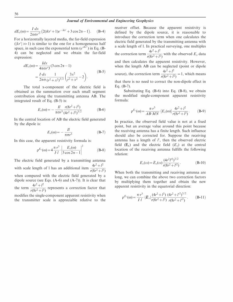
For a horizontally layered media, the far-field expression

( kr’j jww1) is similar to the one for a homogeneous half

space, in such case the exponential term (e-ikr9) in Eq. (B-

4) can be neglected and we obtain the far-fieldexpression:

dEx(v)~Idx

4psr03(3 cos 2a{1)

~I :dx

2ps

1

(r2zx2)3=2

3x2

r2zx2{2

� �:

ðB-5Þ

The total x-component of the electric field isobtained as the summation over each small segment

contribution along the transmitting antenna AB. The

integrated result of Eq. (B-5) is:

Ex(v)~{Il

psr3

r(8r2zl2)

(4r2zl2)3=2ðB-6Þ

In the central location of AB the electric field generated

by the dipole is:

Ex(v)~{Il

psr3ðB-7Þ

In this case, the apparent resistivity formula is:

rEx (v)~4p:r3

I :l: Ex(v)

3 cos 2a{1

��2

ðB-8Þ

The electric field generated by a transmitting antenna

with scale length of l has an additional item4r2zl2

r(8r2zl2)

when compared with the electric field generated by a

dipole source (see Eqs. (A-6) and (A-7)). It is clear that

the term4r2zl2

r(8r2zl2)represents a correction factor that

modifies the single-component apparent resistivity when

the transmitter scale is appreciable relative to the

receiver offset. Because the apparent resistivity is

defined by the dipole source, it is reasonable to

introduce the correction term when one calculates the

electric field generated by the transmitting antenna with

a scale length of l. In practical surveying, one multiples

the correction term4r2zl2

r(8r2zl2)with the observed Ex data

and then calculates the apparent resistivity. However,

when the length AB can be neglected (point or dipole

source), the correction term4r2zl2

r(8r2zl2)~1, which means

that there is no need to correct the non-dipole effect in

Eq. (B-7).

Substituting Eq. (B-6) into Eq. (B-8), we obtain

the modified single-component apparent resistivity

formula:

rEx (v)~p:r3

AB:MN: Ex(v)½ � 4r2zl2

r(8r2zl2): ðB-9Þ

In practice, the observed field value is not at a fixed

point, but an average value around this point because

the receiving antenna has a finite length. Such influence

should also be corrected for. Suppose the receiving

antenna has a length of l9, then the observed electric

field (EEx) and the electric field (Ex) at the central

location of the receiving antenna fulfills the following

relation:

Ex(v)~E�

x(v)(4r2l02)3=2

r(8r2zl02): ðB-10Þ

When both the transmitting and receiving antenna are

long, we can combine the above two correction factors

by multiplying them together and obtain the new

apparent resistivity in the equatorial direction:

rEx (v)~p:r3

I :l: �EExj j

(4r2zl2)

r(8r2zl2)

(4r2zl’2)3=2

r(8r2zl’2): ðB-11Þ

56


discovery of a major coal deposit in china with the use of ... · discovery of a major coal deposit...

Documents